Munich Personal RePEc Archive Efficient estimation of Markov regime-switching models: An application to electricity wholesale market prices Rafal Weron and Joanna Janczura Institute of Organization and Management, Wroclaw University of Technology November 2010 Online at https://mpra.ub.uni-muenchen.de/26628/ MPRA Paper No. 26628, posted 11. November 2010 10:45 UTC
Transcript
MPRAMunich Personal RePEc Archive
Efficient estimation of Markovregime-switching models: An applicationto electricity wholesale market prices
Rafal Weron and Joanna Janczura
Institute of Organization and Management, Wroc law University ofTechnology
November 2010
Online at https://mpra.ub.uni-muenchen.de/26628/MPRA Paper No. 26628, posted 11. November 2010 10:45 UTC
Abstract: In this paper we discuss the calibration issues of models built onmean-reverting processes combined with Markov switching. Due to the unob-servable switching mechanism, estimation of Markov regime-switching (MRS)models requires inferring not only the model parameters but also the state pro-cess values at the same time. The situation becomes more complicated when theindividual regimes are independent from each other and at least one of themexhibits temporal dependence (like mean reversion in electricity spot prices).Then the temporal latency of the dynamics in the regimes has to be taken intoaccount. In this paper we propose a method that greatly reduces the compu-tational burden induced by the introduction of independent regimes in MRSmodels. We perform a simulation study to test the efficiency of the proposedmethod and apply it to a sample series of wholesale electricity spot prices fromthe German EEX market. The proposed 3-regime MRS model fits this data welland also contains unique features that allow for useful interpretations of the pricedynamics.
AMS 2000 subject classifications: Primary 62M05; secondary 60J60.Keywords and phrases: Markov regime-switching, heteroskedasticity, EM al-gorithm, independent regimes, electricity spot price.
1. Introduction
During the last two decades the structure of the power industry has changed dra-matically worldwide. The vertically integrated, monopolistic organizations have beenreplaced by deregulated, competitive markets. The wholesale spot electricity prices –now driven by demand (from utilities serving the households and firms) and supply(from generators) and set on an hourly or half-hourly basis – have recorded unseenearlier levels and extreme volatility. In several cases, severe weather conditions, oftenin combination with exercise of market power by some players, led to unprecedented
price fluctuations – ranging even two orders of magnitude within a matter of hoursor days. Just recall the California crisis of 2000/2001, the early and harsh winterof 2002/2003 following a dry autumn in Scandinavia or the extreme price spikes inJanuary-March 2008 in South Australia in the midst of Australian summer.
Apparently, the deregulation process has created a situation where generators,marketeers and utilities alike are exposed to substantial financial risks. This in turnhas propelled research in quantitative modeling for the power markets (for reviewssee e.g. Benth et al., 2008; Huisman, 2009; Weron, 2006). Parsimonious, yet realisticelectricity price models have become the focus of the trading and risk managementdepartments in many companies and financial institutions.
However, when building realistic models we cannot forget about the uniquenessof electricity as a commodity. It cannot be stored economically and requires imme-diate delivery. At the same time end-user demand shows high variability and strongweather and business cycle dependence. Effects like power plant outages, transmis-sion grid (un)reliability and strategic bidding add complexity and randomness. Theresulting spot prices exhibit strong seasonality on the annual, weekly and daily level,as well as, mean reversion, very high volatility and abrupt, short-lived and generallyunanticipated extreme price spikes or drops (De Jong, 2006; Janczura and Weron,2010; Karakatsani and Bunn, 2008). What classes of models should we then use toefficiently describe electricity spot price dynamics?
Mean-reverting diffusion-type processes, like the Vasicek (1977) model and the CIR(or square root) process of Cox et al. (1985), were at the heart of interest rate mod-eling for years. Their parsimony – often referred to as ‘reduced-form’ – together withtheir ability to represent mean reversion made them models of first choice also in elec-tricity spot price modeling (Barz and Johnson, 1998; Kaminski, 1997). By includinga Poisson jump component the mean-reverting jump-diffusion (MRJD) models wereable to address the two main characteristics of electricity prices – mean reversion andjumps. However, not adequately. A serious flaw of MRJD models is the slow speed ofmean reversion after a jump. When electricity prices spike, they tend to return to theirmean reversion levels much faster than when they suffer smaller shocks. However, ahigh rate of mean reversion, required to force the price back to its normal level after ajump, would lead to a highly overestimated mean reversion rate for prices outside the‘spike regime’. A number of authors have tried to address this flaw (introducing signedjumps, two rates of mean reversion, etc.), but with moderate success (Weron, 2006).Another weakness of MRJD models is their inability to yield consecutive spikes withthe frequency observed in market data, see Figure 1 where two sample spot price tra-jectories are plotted (for more evidence and discussions see Christensen et al., 2009;Janczura and Weron, 2010).
A different line of models originated with the papers of Deng (1998) and Ethier and Mount(1998), who suggested to use the Markov regime-switching (MRS; or Markov-switching,MS) mechanism in the context of electricity prices. Unlike jump-diffusions, MRS mod-els allow for consecutive spikes in a very natural way. Also the return of prices aftera spike to the ‘normal’ regime is straightforward, as the MRS mechanism admitstemporal changes of model dynamics. While it is clear that MRS models have anedge over jump-diffusions, it may not be obvious why favor them over threshold typeregime-switching models or hidden Markov models. Let us elaborate on this briefly.
/ 3
Oct 13 2007 Nov 13, 2007 Dec 13, 2007
40
60
80
100
120
140
NE
PO
OL
pric
e [U
SD
/MW
h]
Days
PriceSpikeDrop
Jul 16, 2006 Aug 16, 2006 Sep 16, 2006
20
40
60
80
100
120
EE
X p
rice
[EU
R/M
Wh]
Days
PriceSpikeDrop
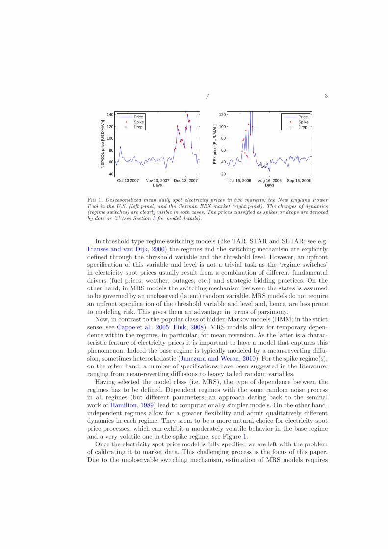
Fig 1. Deseasonalized mean daily spot electricity prices in two markets: the New England PowerPool in the U.S. (left panel) and the German EEX market (right panel). The changes of dynamics(regime switches) are clearly visible in both cases. The prices classified as spikes or drops are denotedby dots or ’x’ (see Section 5 for model details).
In threshold type regime-switching models (like TAR, STAR and SETAR; see e.g.Franses and van Dijk, 2000) the regimes and the switching mechanism are explicitlydefined through the threshold variable and the threshold level. However, an upfrontspecification of this variable and level is not a trivial task as the ‘regime switches’in electricity spot prices usually result from a combination of different fundamentaldrivers (fuel prices, weather, outages, etc.) and strategic bidding practices. On theother hand, in MRS models the switching mechanism between the states is assumedto be governed by an unobserved (latent) random variable. MRS models do not requirean upfront specification of the threshold variable and level and, hence, are less proneto modeling risk. This gives them an advantage in terms of parsimony.
Now, in contrast to the popular class of hidden Markov models (HMM; in the strictsense, see Cappe et al., 2005; Fink, 2008), MRS models allow for temporary depen-dence within the regimes, in particular, for mean reversion. As the latter is a charac-teristic feature of electricity prices it is important to have a model that captures thisphenomenon. Indeed the base regime is typically modeled by a mean-reverting diffu-sion, sometimes heteroskedastic (Janczura and Weron, 2010). For the spike regime(s),on the other hand, a number of specifications have been suggested in the literature,ranging from mean-reverting diffusions to heavy tailed random variables.
Having selected the model class (i.e. MRS), the type of dependence between theregimes has to be defined. Dependent regimes with the same random noise processin all regimes (but different parameters; an approach dating back to the seminalwork of Hamilton, 1989) lead to computationally simpler models. On the other hand,independent regimes allow for a greater flexibility and admit qualitatively differentdynamics in each regime. They seem to be a more natural choice for electricity spotprice processes, which can exhibit a moderately volatile behavior in the base regimeand a very volatile one in the spike regime, see Figure 1.
Once the electricity spot price model is fully specified we are left with the problemof calibrating it to market data. This challenging process is the focus of this paper.Due to the unobservable switching mechanism, estimation of MRS models requires
/ 4
inferring not only the model parameters but also the state process values at the sametime. The situation becomes even more complicated when the individual regimes areindependent from each other but at least one of them is mean-reverting. Then thetemporal latency of the dynamics in the regimes has to be taken into account. In thispaper we propose a method that greatly reduces the computational burden inducedby the introduction of independent regimes in MRS models. Since the latter can beconsidered as generalizations of HMMs (Cappe et al., 2005), this result can have far-reaching implications for many problems where HMMs have been applied (see e.g.Mamon and Elliott, 2007; Scharpf et al., 2008; Shirley et al., 2010).
The paper is structured as follows. In Section 2 we define the MRS models usedin this paper. Next, in Section 3 we describe the estimation procedure for parameter-switching models and introduce an approximation to avoid the computational burdenin case of independent regimes. In Section 4 a simulation study to test the performanceof the proposed method is summarized. Then, in Section 5 an application of theproposed approach to models of wholesale electricity prices is discussed. Finally, inSection 6 we conclude.
2. The models
The underlying idea behind Markov regime-switching (MRS; or hidden Markov mod-els – HMM) is to represent the observed stochastic behavior of a specific time seriesby two (or more) separate states or regimes with different underlying stochastic pro-cesses. The switching mechanism between the states is assumed to be an unobserved(latent) Markov chain Rt. It is described by the transition matrix P containing theprobabilities pij = P (Rt+1 = j | Rt = i) of switching from regime i at time t toregime j at time t + 1. For instance, for i, j = {1, 2} we have:
P = (pij) =
(
p11 p12
p21 p22
)
=
(
1 − p12 p12
p21 1 − p21
)
. (2.1)
Because of the Markov property the current state Rt at time t depends on the pastonly through the most recent value Rt−1.
In this paper we focus on two specifications of MRS models popular in the energyeconomics literature (see e.g. De Jong, 2006; Janczura and Weron, 2010; Mount et al.,2006). Both are based on a discretized version of the mean-reverting, heteroskedasticprocess given by the following SDE:
dXt = (α − βXt)dt + σ|Xt|γdWt. (2.2)
Note, that the absolute value is needed if negative data is analyzed.In the first specification only the model parameters change depending on the state
process values, while in the second the individual regimes are driven by independentprocesses. More precisely, in the first case the observed process Xt is described by aparameter-switching times series of the form:
Xt = αRt+ (1 − βRt
)Xt−1 + σRt|Xt−1|γRt ǫt, (2.3)
/ 5
sharing the same set of random innovations in both regimes (ǫt’s are assumed to beN(0, 1)-distributed). In the second one, Xt is defined as:
Xt =
{
Xt,1 if Rt = 1,Xt,2 if Rt = 2,
(2.4)
where at least one regime is given by:
Xt,i = αi + (1 − βi)Xt−1,i + σi|Xt−1,i|γiǫt,i, i = 1 ∨ i = 2. (2.5)
Note, that here we focus on a 2-regime model, but it is straightforward to generalizeall the results of this paper to a model with 3 or more regimes.
3. Model calibration
Calibration of MRS models is not straightforward since the regimes are only la-tent and hence not directly observable. Hamilton (1990) introduced an applicationof the Expectation-Maximization (EM) algorithm of Dempster et al. (1977), wherethe whole set of parameters θ is estimated by an iterative two-step procedure. Thealgorithm was later refined by Kim (1994). In Section 3.1 we briefly describe thegeneral estimation procedure and provide explicit formulas for the model defined byeqn. (2.3). Next, in Section 3.2 we discuss the computational problems induced bythe introduction of independent regimes, see eqns. (2.4) and (2.5), and propose anefficient remedy.
3.1. Parameter-switching variant
The algorithm starts with an arbitrarily chosen vector of initial parameters θ(0) =
(α(0)i , β
(0)i , σ
(0)i , γ
(0)i , P(0)), for i = 1, 2, see equations (2.1), (2.3) and (2.5). In the
first step of the iterative procedure (the E-step) inferences about the state processare derived. Since Rt is latent and not directly observable, only the expected val-ues of the state process, given the observation vector E(IRt=i|x1, x2..., xT ; θ), can becalculated. These expectations result in the so called ‘smoothed inferences’, i.e. theconditional probabilities P (Rt = j|x1, ..., xT ; θ) for the process being in regime j attime t. Next, in the second step (the M-step) new maximum likelihood (ML) estimatesof the parameter vector θ, based on the smoothed inferences obtained in the E-step,are calculated. Both steps are repeated until the (local) maximum of the likelihoodfunction is reached. A detailed description of the algorithm is given bellow.
3.1.1. The E-step
Assume that θ(n) is the parameter vector calculated in the M-step during the previousiteration. Let xt = (x1, x2, ...xt). The E-part consists of the following steps (Kim,1994):
/ 6
i) Filtering: based on the Bayes rule for t = 1, 2, ..., T iterate on equations:
P (Rt = i|xt; θ(n)) =
P (Rt = i|xt−1; θ(n))f(xt|Rt = i; xt−1; θ
(n))2∑
i=1
P (Rt = i|xt−1; θ(n))f(xt|Rt = i; xt−1; θ(n))
,
where f(xt|Rt = i; xt−1; θ(n)) is the density of the underlying process at time t
conditional that the process was in regime i (i ∈ 1, 2),
and
P (Rt+1 = i|xt; θ(n)) =
2∑
j=1
p(n)ji P (Rt = j|xt; θ
(n)),
until P (RT = i|xT ; θ(n)) is calculated.
ii) Smoothing: for t = T − 1, T − 2, ..., 1 iterate on
P (Rt = i|xT ; θ(n)) =
2∑
j=1
P (Rt = i|xt; θ(n))P (Rt+1 = j|xT ; θ(n))p
(n)ij
P (Rt+1 = i|xt; θ(n)).
The above procedure requires derivation of f(xt|Rt = i; xt−1; θ(n)) used in the
filtering part i). Observe, that the model definition (2.3) implies that Xt given Xt−1
has a conditional Gaussian distribution with mean αi + (1 − βi)Xt−1 and standarddeviation σi|Xt−1|γi given by the following probability distribution function (pdf):
f(
xt|Rt = i; xt−1; θ(n)
)
=1
√2πσ
(n)i |xt−1|γ
(n)i
·
· exp
−
(
xt −(
1 − β(n)i
)
xt−1 − α(n)i
)2
2(
σ(n)i
)2
|xt−1|2γi(n)
. (3.1)
3.1.2. The M-step
In the second step of the EM algorithm, new and more exact maximum likelihood(ML) estimates θ(n+1) for all model parameters are calculated. Compared to standard
ML estimation, where for a given pdf f the log-likelihood function∑T
t=1 log f(xt, θ(n))
is maximized, here each component of this sum has to be weighted with the corre-sponding smoothed inference, since each observation xt belongs to the ith regimewith probability P (Rt = i|xT ; θ(n)). In particular, for the model defined by eqn. (2.3)explicit formulas for the estimates are provided in the following lemma.
Lemma 3.1. The ML estimates for the parameters of the model defined by (2.3) are
/ 7
given by the following formulas:
αi =
T∑
t=2
[
P (Rt = i|xT ; θ(n))|xt−1|−2γi(xt − (1 − βi)xt−1)]
T∑
t=2
[
P (Rt = i|xT ; θ(n))|xt−1|−2γi
]
,
βi =
T∑
t=2
{
P (Rt = i|xT ; θ(n))xt−1|xt−1|−2γiB1
}
T∑
t=2
[
P (Rt = i|xT ; θ(n))xt−1|xt−1|−2γiB2
]
,
B1 = xt − xt−1 −∑T
t=2 P (Rt = i|xT ; θ(n))|xt−1|−2γi (xt − xt−1)∑T
t=2 P (Rt = i|xT ; θ(n))|xt−1|−2γi
,
B2 =
∑Tt=2 P (Rt = i|xT ; θ(n))xt−1|xt−1|−2γi
∑Tt=2 P (Rt = i|xT ; θ(n))|xt−1|−2γi
− xt−1,
σ2i =
T∑
t=2
{
P (Rt = i|xT ; θ(n))|xt−1|−2γi(xt − αi − (1 − βi)xt−1)}2
T∑
t=2P (Rt = i|xT ; θ(n))
.
The fourth parameter, γi, requires numerical maximization of the likelihood function.
Finally, in the last part of the M-step the transition probabilities are estimatedaccording to the following formula (Kim, 1994):
p(n+1)ij =
T∑
t=2P (Rt = j, Rt−1 = i|xT ; θ(n))
T∑
t=2P (Rt−1 = i|xT ; θ(n))
= (3.2)
=
T∑
t=2P (Rt = j|xT ; θ(n))
p(n)ij
P (Rt−1=i|xt−1;θ(n))
P (Rt=j|xt−1);θ(n)
T∑
t=2P (Rt−1 = i|xT ; θ(n))
,
where p(n)ij is the transition probability from the previous iteration. All values obtained
in the M-step are then used as a new parameter vector θ(n+1) = (αi, βi, σi, γi, P(n+1)),
i = 1, 2, in the next iteration of the E-step.
3.2. Independent regimes variant
In the parameter-switching model (2.3) the current value of the process depends onthe last observation only, no matter which regime it originated from. This implies
/ 8
10 20 30 40 50 60 70
0
2
4
6
8
10
Time
Val
ue
X
t,1X
t,2X
t
Fig 2. A sample trajectory of the MRS model with independent regimes (black solid line) super-imposed on the observable and latent values of the processes in both regimes. The simulation wasperformed for a model with the following parameters: p11 = 0.9, p22 = 0.8, α1 = 1, β1 = 0.7, σ2
1= 1,
γ1 = 0, α2 = 2, β2 = 0.3, σ2
2= 0.01, γ2 = 1.
that for the calculation of the conditional pdf (3.1), used in the i) part of the E-steprecursions, the information from only one preceding time step is needed. Consequently,the EM algorithm requires storing conditional probabilities P (Rt = i|xT ) of one timestep only, i.e. 2T values in total.
However, the estimation procedure complicates significantly, if the regimes areindependent from each other. Observe, that the values of the mean-reverting regimebecome latent when the process is in the other state (see Figure 2 for an illustration).This makes the distribution of Xt dependent on the whole history (x1, x2, ..., xt−1) ofthe process. As a consequence all possible paths of the state process (R1, R2, ..., Rt)should be considered in the estimation procedure, implying that f(xt|Rt = i, Rt−1 6=i, ..., Rt−j 6= i, Rt−j−1 = i; xt−1; θ
(n)) and the whole set of probabilities P (Rt =it, Rt−1 = it−1, ..., Rt−j = it−j |xt−1; θ
(n)) should be used in the E-step. Obviously,this leads to a high computational complexity, as the number of possible state processrealizations is equal to 2T and increases rapidly with the sample size.
As a feasible solution to this problem Huisman and de Jong (2002) suggested touse probabilities of the last 10 observations. Apart from the fact that such an ap-proximation still is computationally intensive, it can be used only if the probabilityof more than 10 consecutive observations from the second regime is negligible.
Instead, we suggest to replace the latent variables xt−1 in formula (3.1) with theirexpectations xt−1 = E(Xt−1|xt−1; θ
(n)) based on the whole information availableat time t − 1. A similar approach was proposed by Gray (1996) in the context ofregime-switching GARCH models to avoid the problem of the conditional standarddeviation path dependence. Now, the estimation procedure described in Section 3.1
/ 9
can be applied with the following approximation of the pdf:
f(
xt|Rt = i; xt−1; θ(n)
)
=1
√2πσ
(n)i |xt−1,i|γ
(n)i
·
· exp
−
(
xt −(
1 − β(n)i
)
xt−1,i − α(n)i
)2
2(
σ(n)i
)2
|xt−1,i|2γi(n)
,(3.3)
where xt,i denotes the expected value of the ith regime at time t, i.e. E(
Xt,i|xt; θ(n)
)
.Note, that compared to formula (3.1) for the parameter-switching variant, the ob-served value of the process xt−1 is now replaced by the expected value xt−1,i of theith regime at time t − 1. The following lemma describes how to derive these values.
Lemma 3.2. Expected values E(
Xt,i|xt; θ(n)
)
are given by the following recursiveformula:
E(
Xt,i|xt; θ(n)
)
= P(
Rt = i|xt; θ(n)
)
xt + P(
Rt 6= i|xt; θ(n)
)
·
·{
α(n)i +
(
1 − β(n)i
)
E(
Xt−1,i|xt−1; θ(n)
)}
.
It is interesting to note, that
E(
Xt,i|xt; θ(n)
)
=t−1∑
k=0
xt−k
(
1 − β(n)i
)k
P(
Rt−k = i|xt−k; θ(n))
·
·k
∏
j=1
P(
Rt−j+1 6= i|xt−j+1; θ(n)
)
+α(n)i
t−1∑
k=0
(
1 − β(n)i
)kk
∏
j=0
P(
Rt−j+1 6= i|xt−j+1; θ(n)
)
.
Hence, the expected value E(Xt,i|xt; θ(n)) is a linear combination of the observed
vector xt and the probabilities P (Rj = i|xj ; θ(n)) calculated during the estimation
procedure (see the filtering part of the E-step). This observation shows that usingxt−1,i = E(Xt−1,i|xt−1; θ
(n)) in formula (3.3) instead of xt−1, as in formula (3.1)for the parameter-switching variant, the computational complexity of the E-step isgreatly reduced.
The estimation procedure described in this section can be applied to models inwhich at least one regime is described by the mean-reverting process given by (2.5).The independent regimes specification is commonly used in the electricity price mod-eling literature (for a recent review see Janczura and Weron, 2010). It is often as-sumed that one regime follows a mean-reverting process, while the values in the otherregime(s) are independent random variables from a specified distribution. The esti-mation steps are then as described above, with the exception that the M-step is nowdependent on the choice of the distribution in the other regime(s). Finally, note thatin MRS models the likelihood function should be weighted with the correspondingprobability (analogously as in the proof of Lemma 3.1, see the Appendix, eqn. (6.2)).
/ 10
Table 1
Means, 95% confidence intervals (CIl,CIu) and standard deviations (Std) of parameter estimatesobtained from 1000 simulated trajectories of 10000 observations each, for the three studied MRS
In order to test the performance of the estimation method proposed in Section 3.2,we provide a simulation study. For each of the following three MRS model types wegenerate 1000 sample trajectories:
• MR: with parameter-switching mean-reverting regimes, see (2.3),• IMR: with independent mean-reverting processes in both regimes, see (2.5),• IMR-G: with a mean-reverting process in the first regime and independent
N(α2, σ22)-distributed random variables in the second regime.
The IMR model is simulated with probabilities of staying in the same regime equal top11 = 0.9 and p22 = 0.8 for the first and the second regime, respectively. With sucha choice of the transition matrix we can expect to see many consecutive observationsin each regime. Indeed, the probability of 10 consecutive observations from the firstregime is equal to 0.35 and even for 40 consecutive observations that probability isstill higher than 0.01. Obviously, such a model cannot be estimated based on theinformation about only a few prevailing observations.
For each sample trajectory we apply one of the estimation procedures describedin Section 3. Then, we calculate the means, standard deviations and 95% confidenceintervals of the parameter estimates. The values obtained for trajectories consistingof 10000 observations are given in Table 1. All sample means are close to the trueparameters with a deviation of no more than 0.03 (in absolute terms). In fact, in mostcases the deviation is significantly lower. Moreover, all parameter values are withinthe obtained 95% confidence intervals. Also the standard deviation of the estimatesis quite low and, except for γ2 and α2 in the IMR model, does not exceed 0.04.
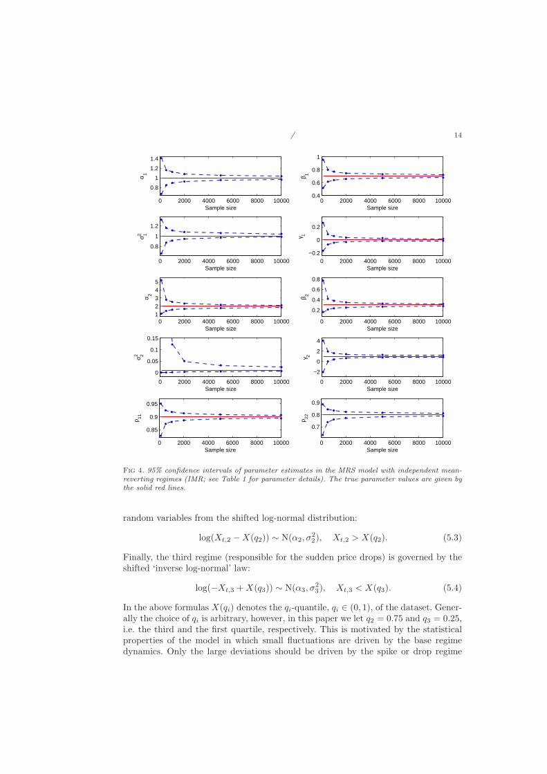
Next, we check how the proposed method works for different sample sizes. We gen-erate MRS model trajectories with 100, 500, 1000, 2000, 5000, and 10000 observations.The obtained means and standard deviations are given in Tables 2 (MR model), 3(IMR model) and 4 (IMR-G model). The respective confidence intervals are plotted inFigures 3, 4 and 5. As expected, the standard deviations, as well as, the width of theconfidence intervals decrease with increasing sample size. Looking at the means, in
/ 11
Table 2
Means and standard deviations (Std), over 1000 simulated trajectories, of parameter estimates inthe MR model calculated for different sample sizes.
most cases a sample of 1000 (or even 500 for the MR and IMR-G models) observationsyields satisfactory results, as the deviation does not exceed 0.03 (in absolute terms).Especially for the IMR-G model the results are very satisfactory. This is importantin view of the fact that a variant of this model is used in Section 5 for modelingelectricity spot prices.
5. Application to electricity spot prices
In this study we present how the techniques introduced in Section 3 can be used to effi-ciently calibrate MRS models to electricity spot prices. We use mean daily (baseload)day-ahead spot prices from the European Energy Exchange (EEX; Germany). Thesample totals 1827 daily observations (or 267 full weeks) and covers the 5-year periodJanuary 3, 2005 – January 3, 2010.
When modeling electricity spot prices we have to bear in mind that electricity isa very specific commodity. Both electricity demand and (to some extent) supply ex-hibit seasonal fluctuations. They mostly arise due to changing climate conditions, liketemperature and the number of daylight hours. These seasonal fluctuations translateinto seasonal behavior of electricity prices, and spot prices in particular. In the mid-and long-term also the fuel price levels (of natural gas, oil, coal) influence electric-ity prices. However, not wanting to focus the paper on modeling the fuel stack/bidstack/electricity spot price relationships, following Janczura and Weron (2010) we will
/ 12
Table 4
Means and standard deviations (Std), over 1000 simulated trajectories, of parameter estimates inthe IMR-G model calculated for different sample sizes.
use a single non-parametric long-term seasonal component (LTSC) to represent thelong-term non-periodic fuel price levels, the changing climate/consumption conditionsthroughout the years and strategic bidding practices.
We assume that the electricity spot price, Pt, can be represented by a sum of twoindependent parts: a predictable (seasonal) component ft and a stochastic compo-nent Xt , i.e. Pt = ft + Xt. Further, we let ft be composed of a weekly periodicpart, st, and a LTSC, Tt. The deseasonalization is then conducted in three steps.First, the long term trend Tt is estimated from daily spot prices Pt using a waveletfiltering-smoothing technique (for details see Truck et al., 2007; Weron, 2006). Thisprocedure, also known as low pass filtering, yields a traditional linear smoother. Herewe use the S6 approximation, which roughly corresponds to bi-monthly (26 = 64 days)smoothing.
The price series without the LTSC is obtained by subtracting the S6 approximationfrom Pt. Next, the weekly periodicity st is removed by subtracting the ‘average week’calculated as the arithmetic mean of prices corresponding to each day of the week(German national holidays are treated as the eight day of the week). Finally, thedeseasonalized prices, i.e. Pt−Tt−st, are shifted so that the mean of the new processis the same as the mean of Pt. The resulting deseasonalized time series Xt = Pt−Tt−st
can be seen in Figure 6.The second well known feature of electricity prices are the sudden, unexpected
price changes, known as spikes or jumps. The ‘spiky’ nature of spot prices is the effectof non-storability of electricity. Electricity to be delivered at a specific hour cannot besubstituted for electricity available shortly after or before. Extreme load fluctuations– caused by severe weather conditions often in combination with generation outagesor transmission failures – can lead to price spikes. On the other hand, an oversupply– due to a sudden drop in demand and technical limitations of an instant shut-down of a generator – can cause price drops. Further, electricity spot prices are ingeneral regarded to be mean-reverting and exhibit the so called ‘inverse leverageeffect’, meaning that the positive shocks increase volatility more than the negativeshocks (Knittel and Roberts, 2005).
Motivated by these facts and the recent findings of Janczura and Weron (2010) welet the stochastic component Xt be driven by a Markov regime-switching model with
/ 13
0 2000 4000 6000 8000 10000
0.5
1
1.5
α 1
Sample size0 2000 4000 6000 8000 10000
0.5
0.6
0.7
0.8
0.9
β 1
Sample size
0 2000 4000 6000 8000 10000
0.5
1
1.5
σ2 1
Sample size0 2000 4000 6000 8000 10000
−0.2
0
0.2
0.4
γ 1
Sample size
0 2000 4000 6000 8000 10000
1.99
2
2.01
α 2
Sample size0 2000 4000 6000 8000 10000
0.28
0.3
0.32
0.34
β 2
Sample size
0 2000 4000 6000 8000 100000
0.01
0.02
σ2 2
Sample size0 2000 4000 6000 8000 10000
0.81
1.21.41.6
γ 2
Sample size
0 2000 4000 6000 8000 10000
0.4
0.5
0.6
p 11
Sample size0 2000 4000 6000 8000 10000
0.4
0.5
0.6
p 22
Sample size
Fig 3. 95% confidence intervals of parameter estimates in the MRS model with parameter-switchingmean-reverting regimes (MR; see Table 1 for parameter details). The true parameter values aregiven by the solid red lines.
three independent states:
Xt =
Xt,1 if Rt = 1,Xt,2 if Rt = 2,Xt,3 if Rt = 3.
(5.1)
The first (base) regime describes the ‘normal’ price behavior and is given by themean-reverting, heteroskedastic process of the form:
where ǫt is the standard Gaussian noise. The second regime represents the suddenprice jumps (spikes) caused by unexpected supply shortages and is given by i.i.d.
/ 14
0 2000 4000 6000 8000 10000
0.8
1
1.2
1.4
α 1
Sample size0 2000 4000 6000 8000 10000
0.4
0.6
0.8
1
β 1
Sample size
0 2000 4000 6000 8000 10000
0.8
1
1.2
σ2 1
Sample size0 2000 4000 6000 8000 10000
−0.2
0
0.2
γ 1
Sample size
0 2000 4000 6000 8000 1000012345
α 2
Sample size0 2000 4000 6000 8000 10000
0.2
0.4
0.6
0.8
β 2
Sample size
0 2000 4000 6000 8000 10000
0
0.05
0.1
0.15
σ2 2
Sample size0 2000 4000 6000 8000 10000
−2
0
2
4
γ 2
Sample size
0 2000 4000 6000 8000 10000
0.85
0.9
0.95
p 11
Sample size0 2000 4000 6000 8000 10000
0.7
0.8
0.9
p 22
Sample size
Fig 4. 95% confidence intervals of parameter estimates in the MRS model with independent mean-reverting regimes (IMR; see Table 1 for parameter details). The true parameter values are given bythe solid red lines.
random variables from the shifted log-normal distribution:
In the above formulas X(qi) denotes the qi-quantile, qi ∈ (0, 1), of the dataset. Gener-ally the choice of qi is arbitrary, however, in this paper we let q2 = 0.75 and q3 = 0.25,i.e. the third and the first quartile, respectively. This is motivated by the statisticalproperties of the model in which small fluctuations are driven by the base regimedynamics. Only the large deviations should be driven by the spike or drop regime
/ 15
0 2000 4000 6000 8000 10000
0.9
1
1.1
α 1
Sample size0 2000 4000 6000 8000 10000
0.6
0.7
0.8
β 1
Sample size
0 2000 4000 6000 8000 10000
0.4
0.5
0.6
0.7
σ2 1
Sample size0 2000 4000 6000 8000 10000
0.4
0.6
0.8
γ 1
Sample size
0 2000 4000 6000 8000 10000
6.8
7
7.2
α 2
Sample size0 2000 4000 6000 8000 10000
0.2
0.4
0.6
σ2 2
Sample size
0 2000 4000 6000 8000 10000
0.75
0.8
0.85
p 11
Sample size0 2000 4000 6000 8000 10000
0.1
0.2
0.3
p 22
Sample size
Fig 5. 95% confidence intervals of parameter estimates in the MRS model with a mean-revertingregime combined with independent Gaussian random variables (IMR-G; see Table 1 for parameterdetails). The true parameter values are given by the solid red lines.
dynamics, which implies that the spike (drop) regime distribution should have massconcentrated well above (below) the median.
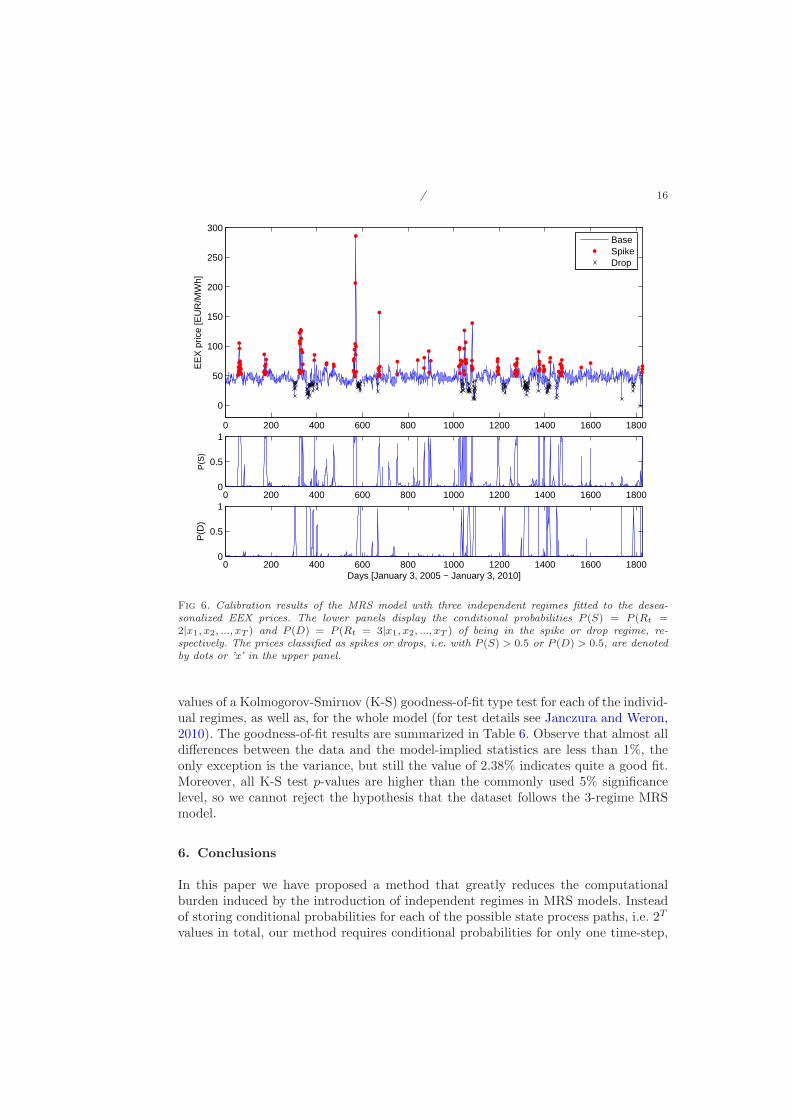
The deseasonalized prices Xt and the conditional probabilities of being in thespike P (Rt = 2|x1, x2, ..., xT ) or drop P (Rt = 3|x1, x2, ..., xT ) regime for the analyzeddataset are displayed in Figure 6. The prices classified as spikes or drops, i.e. withP (Rt = 2|x1, x2, ..., xT ) > 0.5 or P (Rt = 3|x1, x2, ..., xT ) > 0.5, are additionallydenoted by dots or ’x’. The estimated model parameters are given in Table 5.
The obtained base regime parameters are consistent with the well known propertiesof electricity prices. Positive γ is responsible for the ‘inverse leverage effect’, whileβ = 0.42 indicates a high speed of mean-reversion. Considering probabilities of stayingin the same regime pii we obtain quite high values for each of the regimes, rangingfrom 0.65 for the spike regime up to 0.96 for the base regime. As a consequence, onaverage there are many consecutive observations from the same regime.
In order to check the statistical adequacy of the chosen MRS model we calcu-late percentage differences between the data and the model implied moments andquantiles. The model implied values are obtained as the mean value of the statisticscalculated over 1000 simulated trajectories. A negative sign indicates that the valueobtained from the dataset is lower than the model-implied. Moreover, we report the p-
/ 16
0 200 400 600 800 1000 1200 1400 1600 1800
0
50
100
150
200
250
300
EE
X p
rice
[EU
R/M
Wh]
BaseSpikeDrop
0 200 400 600 800 1000 1200 1400 1600 18000
0.5
1
P(S
)
0 200 400 600 800 1000 1200 1400 1600 18000
0.5
1
P(D
)
Days [January 3, 2005 − January 3, 2010]
Fig 6. Calibration results of the MRS model with three independent regimes fitted to the desea-sonalized EEX prices. The lower panels display the conditional probabilities P (S) = P (Rt =2|x1, x2, ..., xT ) and P (D) = P (Rt = 3|x1, x2, ..., xT ) of being in the spike or drop regime, re-spectively. The prices classified as spikes or drops, i.e. with P (S) > 0.5 or P (D) > 0.5, are denotedby dots or ’x’ in the upper panel.
values of a Kolmogorov-Smirnov (K-S) goodness-of-fit type test for each of the individ-ual regimes, as well as, for the whole model (for test details see Janczura and Weron,2010). The goodness-of-fit results are summarized in Table 6. Observe that almost alldifferences between the data and the model-implied statistics are less than 1%, theonly exception is the variance, but still the value of 2.38% indicates quite a good fit.Moreover, all K-S test p-values are higher than the commonly used 5% significancelevel, so we cannot reject the hypothesis that the dataset follows the 3-regime MRSmodel.
6. Conclusions
In this paper we have proposed a method that greatly reduces the computationalburden induced by the introduction of independent regimes in MRS models. Insteadof storing conditional probabilities for each of the possible state process paths, i.e. 2T
values in total, our method requires conditional probabilities for only one time-step,
/ 17
Table 5
Calibration results of the MRS model with three independent regimes fitted to the deseasonalizedEEX prices
Goodness-of-fit statistics for the 3-regime MRS model fitted to the deseasonalized EEX prices. Formoments and quantiles the relative differences between the sample and the model implied statistics
are given (the latter are obtained from 1000 simulations).
Moments Quantiles K-S test p-values
E(X) Var(X) 0.1 0.25 0.5 0.75 0.9 Base Spike Drop Model
i.e. 2T values. We have performed a limited simulation study to test the efficiency ofthe new method and applied it to a sample series of electricity spot prices.
The simulation study has shown that all sample means are close to the true pa-rameter values (and all true parameter values are within the obtained 95% confidenceintervals). Moreover, the standard deviations, as well as, the width of the confidenceintervals decrease with increasing sample size. Looking at the means, in most casesa sample of 1000 (or even 500 for the MR and IMR-G models; for model acronymsand definitions see Section 4) observations yields satisfactory results, as the devia-tion does not exceed 0.03 (in absolute terms). Especially for the IMR-G model theresults are very satisfactory. This is important in view of the fact that variants ofthis model are popular in the energy finance literature. In particular, a model of thistype (with shifted log-normal spike and price drop regimes independent from the basemean-reverting regime) is calibrated in Section 5 to a sample series of deseasonalizedwholesale electricity spot prices from the German EEX market.
The proposed MRS model fits market data well and also contains unique featuresthat allow for useful interpretations of the price dynamics. In particular, the parameterγ can be treated as a parameter representing the ‘degree of inverse leverage’. A positivevalue (e.g. γ1 = 0.70 as in Table 5) indicates ‘inverse leverage’. Recall, that the‘inverse leverage effect’ reflects the observation that positive electricity price shocksincrease volatility more than negative shocks. Knittel and Roberts (2005) attributedthis phenomenon to the fact that a positive shock to electricity prices can be treated asan unexpected positive demand shock. Therefore, as a result of convex marginal costs,positive demand shocks have a larger impact on price changes relative to negativeshocks.
Finally, since MRS models can be considered as generalizations of HMMs, theresults of this paper can have far-reaching implications for many problems whereHMMs have been applied (see e.g. Mamon and Elliott, 2007; Scharpf et al., 2008;Shirley et al., 2010). In some cases, perhaps, a MRS model with independent regimeswould constitute a more realistic model of the observed phenomenon than a HMM.
/ 18
Appendix
Proof of Lemma 3.1. Observe that the joint density f(x1, x2, ..., xT ) can be writtenas a product of appropriate conditional densities
Moreover, Xt conditional on xt−1, xt−2, ..., x1 has a Gaussian distribution with mean(1 − βi)xt−1 + αi and standard deviation σ2
i |xt−1|γi . Thus, the ith regime weightedlog-likelihood function is given by the following formula:
ln[L(αi, βi, σi, γi)] = −T
∑
t=2
P (Rt = i|xT ; θ(n)) ·
·[
ln(√
2πσi|xt−1|γi
)
+(xt − (1 − βi) xt−1 − αi)
2
2σ2i |xt−1|2γi
]
.(6.2)
Note, that the parameter vector θ(n) is omitted in what follows to simplify the nota-tion. In order to find the maximum likelihood (ML) estimates, the partial derivativesof ln(L) are set to zero. This leads to the following system of equations:
T∑
t=2
P (Rt = i|xT )|xt−1|−2γi (xt − (1 − βi)xt−1 − αi) = 0,
T∑
t=2
P (Rt = i|xT )xt−1|xt−1|2γi (xt − (1 − βi)xt−1 − αi) = 0,
T∑
t=2
P (Rt = i|xT )|xt−1|−2γi (xt − (1 − βi)xt−1 − αi)2
=
= σ2i
T∑
t=2
P (Rt = i|xT ),
T∑
t=2
P (Rt = i|xT )|xt−1|−2γi ln |xt−1| (xt − (1 − βi)xt−1 − αi)2
=
= σ2i
T∑
t=2
P (Rt = i|xT ) ln |xt−1|.
/ 19
Now, the ML estimates for αi, βi, and σ2i can be explicitly derived:
where Ix is the indicator function. Taking the expected value conditional on Xt yields:
E(
Xt,i|Xt; θ(n)
)
= P(
Rt = i|Xt; θ(n)
)
Xt + P(
Rt 6= i|Xt; θ(n)
) [
α(n)i +
+(
1 − β(n)i
)
E(
Xt−1,i|Xt, Rt 6= i; θ(n))
+
+σ(n)i E
(
|Xt−1,i|γ(n)i ǫt|Xt, Rt 6= i; θ(n)
)]
.
Since Xt−1,i and ǫt are independent of the σ-algebra generated by {Xt, Rt 6= i} wehave
E(
|Xt−1,i|γ(n)i ǫt|Xt, Rt 6= i; θ(n)
)
= E(
|Xt−1,i|γ(n)i ǫt|Xt−1; θ
(n))
,
andE
(
Xt−1,i|Xt, Rt 6= i; θ(n))
= E(
Xt−1,i|Xt−1; θ(n)
)
.
Moreover, from the law of iterated expectation and basic properties of conditional
/ 20
expected values:
E(
|Xt−1,i|γ(n)i ǫt|Xt−1; θ
(n))
=
= E[
E(
|Xt−1,i|γ(n)i ǫt|Xt−1,Xt−1,i; θ
(n))
|Xt−1; θ(n)
]
=
= E[
|Xt−1,i|γ(n)i E
(
ǫt|Xt−1,Xt−1,i; θ(n)
)
|Xt−1; θ(n)
]
=
= E[
|Xt−1,i|γ(n)i E(ǫt)|Xt−1; θ
(n)]
= 0,
which implies
E(
Xt,i|Xt; θ(n)
)
= P (Rt = i|Xt; θ(n))Xt + P (Rt 6= i|Xt; θ
(n)) ·
·[
α(n)i + (1 − β
(n)i )E
(
Xt−1,j |Xt−1; θ(n)
)]
.
Finally, substituting the variables Xt with their observations xt completes the proof.
References
Barz, G., Johnson, B. (1998). Modeling the prices of commodities that are costlyto store: The case of electricity. Proceedings of the Chicago Risk ManagementConference.
Benth, F.E., Benth, J.S., Koekebakker, S. (2008). Stochastic Modeling of Electricityand Related Markets. World Scientific, Singapore.
Cappe, O., Moulines E., Ryden T. (2005). Inference in Hidden Markov Models.Springer.
Christensen, T., Hurn, S., Lindsay, K. (2009). It never rains but it pours: modelingthe persistence of spikes in electricity prices. The Energy Journal 30(1), 25-48.
Cox, J.C., Ingersoll, J.E., Ross, S.A. (1985). A theory of the term structure of interestrates. Econometrica 53, 385-407.
De Jong, C. (2006). The nature of power spikes: A regime-switch approach. Studiesin Nonlinear Dynamics & Econometrics 10(3), Article 3.
Dempster, A., Laird, N., Rubin, D.B. (1977). Maximum likelihood from incompletedata via the EM algorithm. Journal of the Royal Statistical Society 39, 1-38.
Deng, S.-J. (1998). Stochastic models of energy commodity prices and their applica-tions: Mean-reversion with jumps and spikes. PSerc Working Paper 98-28.
Ethier, R., Mount, T., (1998). Estimating the volatility of spot prices in restructuredelectricity markets and the implications for option values. PSerc Working Paper98-31.
Fink, G.A. (2008). Markov Models for Pattern Recognition: From Theory to Appli-cations. Springer.
Franses, P.H., van Dijk, D. (2000). Nonlinear Time Series Models in Empirical Fi-nance. Cambridge University Press.
Gray, S.F. (1996). Modeling the conditional distribution of interest rates as a regime-switching process. Journal of Financial Economics 42, 27-62.
/ 21
Hamilton, J. (1989). A new approach to the economic analysis of nonstationary timeseries and the business cycle. Econometrica 57, 357-384.
Hamilton, J. (1990). Analysis of time series subject to changes in regime. Journal ofEconometrics 45, 39-70.
Huisman, R. (2009). An Introduction to Models for the Energy Markets. Risk Books.Huisman, R., de Jong, C. (2002). Option formulas for mean-reverting power prices
with spikes. ERIM Report Series Reference No. ERS-2002-96-F&A.Janczura, J., Weron, R. (2010). An empirical comparison of alternate regime-switching
models for electricity spot prices. Energy Economics 32, 1059-1073.Janczura, J., Weron, R. (2010). Goodness-of-fit testing for regime-switching models.
Working paper. Available at MPRA: http://mpra.ub.uni-muenchen.de/22871.Kaminski, V. (1997). The challenge of pricing and risk managing electricity deriva-
tives. In: The US Power Market. Risk Books.Karakatsani, N.V., Bunn, D.W. (2008). Intra-day and regime-switching dynamics in
electricity price formation. Energy Economics 30, 1776-1797.Kim, C.-J. (1994). Dynamic linear models with Markov-switching. J. Econometrics
60, 1-22.Knittel, C.R., Roberts, M.R. (2005). An empirical examination of restructured elec-
tricity prices. Energy Economics 27, 791-817.Mamon, R.S., Elliott, R.J., eds. (2007). Hidden Markov Models in Finance. Interna-
tional Series in Operations Research & Management Science, Vol. 104, Springer.Mount, T.D., Ning, Y., Cai, X. (2006). Predicting price spikes in electricity markets
using a regime-switching model with time-varying parameters. Energy Economics28: 62-80.
Scharpf, R.B., Parmigiani, G., Pevsner, J., Ruczinski, I. (2008) Hidden Markov modelsfor the assessment of chromosomal alterations using high-throughput SNP arrays.The Annals of Applied Statistics 2(2), 687-713.
Shirley, K.E., Small, D.S., Lynch, K.G., Maisto, S.A., Oslin, D.W. (2010). HiddenMarkov models for alcoholism treatment trial data. The Annals of Applied Statistics4(1), 366-395.
Truck, S., Weron, R., Wolff, R. (2007). Outlier treatment and robust approaches formodeling electricity spot prices. Proceedings of the 56th Session of the ISI. Availableat MPRA: http://mpra.ub.uni-muenchen.de/4711/.
Vasicek, O. (1977). An equilibrium characterization of the term structure. Journal ofFinancial Economics 5, 177-188.
Weron, R. (2006). Modeling and forecasting electricity loads and prices: A statisticalapproach. Wiley, Chichester.
Weron, R. (2009). Heavy-tails and regime-switching in electricity prices. MathematicalMethods of Operations Research 69(3), 457-473.