Patni, M., Minera Rebulla, S. A., Weaver, P. M., & Pirrera, A. (2020). Efficient modelling of beam-like structures with general non-prismatic, curved geometry. Computers and Structures, 240, [106339]. https://doi.org/10.1016/j.compstruc.2020.106339 Peer reviewed version License (if available): CC BY-NC-ND Link to published version (if available): 10.1016/j.compstruc.2020.106339 Link to publication record in Explore Bristol Research PDF-document This is the author accepted manuscript (AAM). The final published version (version of record) is available online via Elsevier at https://doi.org/10.1016/j.compstruc.2020.106339 . Please refer to any applicable terms of use of the publisher. University of Bristol - Explore Bristol Research General rights This document is made available in accordance with publisher policies. Please cite only the published version using the reference above. Full terms of use are available: http://www.bristol.ac.uk/red/research-policy/pure/user-guides/ebr-terms/
Transcript
Patni, M., Minera Rebulla, S. A., Weaver, P. M., & Pirrera, A. (2020).Efficient modelling of beam-like structures with general non-prismatic,curved geometry. Computers and Structures, 240, [106339].https://doi.org/10.1016/j.compstruc.2020.106339
Peer reviewed versionLicense (if available):CC BY-NC-NDLink to published version (if available):10.1016/j.compstruc.2020.106339
Link to publication record in Explore Bristol ResearchPDF-document
This is the author accepted manuscript (AAM). The final published version (version of record) is available onlinevia Elsevier at https://doi.org/10.1016/j.compstruc.2020.106339 . Please refer to any applicable terms of use ofthe publisher.
University of Bristol - Explore Bristol ResearchGeneral rights
This document is made available in accordance with publisher policies. Please cite only thepublished version using the reference above. Full terms of use are available:http://www.bristol.ac.uk/red/research-policy/pure/user-guides/ebr-terms/
Efficient modelling of beam-like structures with general non-prismatic,curved geometry
M. Patnia,∗, S. Mineraa, P. M. Weavera,b, A. Pirreraa
aBristol Composites Institute (ACCIS), Department of Aerospace Engineering, University of Bristol, Queen’s Building,University Walk, Bristol BS8 1TR, UK.
bBernal Institute, School of Engineering, University of Limerick, Castletroy, Ireland.
Abstract
The analysis of three-dimensional (3D) stress states can be complex and computationally expensive, espe-cially when large deflections cause a nonlinear structural response. Slender structures are conventionallymodelled as one-dimensional beams but even these rather simpler analyses can become complicated, e.g. forvariable cross-sections and planforms (i.e. non-prismatic curved beams). In this paper, we present an alter-native procedure based on the recently developed Unified Formulation in which the kinematic descriptionof a beam builds upon two shape functions, one for the beam’s axis, the other for its cross-section. This ap-proach predicts 3D displacement and stress fields accurately and is computationally efficient in comparisonwith 3D finite elements. However, current modelling capabilities are limited to the use of prismatic elements.As a means for further applicability, we propose a method to create beam elements with variable planformand variable cross-section, i.e. of general shape. This method employs an additional set of shape functionswhich describes the geometry of the structure exactly. These functions are different from those used fordescribing the kinematics and provide local curvilinear basis vectors upon which 3D Jacobian transformationmatrices are produced to define non-prismatic elements. The model proposed is benchmarked against 3Dfinite element analyses, as well as analytical and experimental results available in the literature. Significantcomputational efficiency gains over 3D finite elements are observed for similar levels of accuracy, for bothlinear and geometrically nonlinear analyses.
The accuracy and computational efficiency of static linear and nonlinear analyses of variable cross-section,variable planform, i.e. non-prismatic and curved beams is of great importance, particularly in mechanical,civil and aerospace engineering. In order to meet ever more stringent weight and/or efficiency requirements,many applications, such as wings, engine or wind turbine blades, demand the use of advanced compositematerials and highly tailored geometries for functional and/or aerodynamic reasons. Such structures arealso often sized to be slender, thin-walled and include variable-thickness semi-monocoque shells. Ultimately,these features compound to make stress/strength analyses both cumbersome and computationally expensive,which is a problem because accurate analyses are crucial for sizing and optimisation at all design stages.
At early design iterations, one-dimensional (1D) and two-dimensional (2D) finite element models arecommonly employed for their efficiency and relative accuracy. However, their capabilities are limited todescribing general, stiffness-driven, behaviour. For example, thin-shell formulations can predict in-planebending and stretching response fairly well, but recovering local features, such as through-thickness trans-verse stresses or displacement field gradients close to singularities, may not be possible. These details are
Preprint submitted to Computers & Structures July 14, 2020
then addressed only at later stages of the design process by treating the structure as a three-dimensional(3D) continuum, i.e. utilising 3D equilibrium equations and associated point-wise boundary conditions tocompute stresses and deflections. However, there is increasing evidence that localised 3D stress featuresextend their effects far field in sizing optimisation problems, especially when layered, anisotropic materialsand the relevant manufacturing rules are involved [1]. This observation brings the adequacy of simplified,early-iteration models into question. Solving a 3D boundary value problem or employing 3D finite element(FE) models at early design iterations can be time consuming and computationally expensive. Therefore,there is a need to develop an efficient mathematical method that is able of capturing salient displacementand stress features in structures of generic, slender, thin-walled form for incorporation into early-stage designiterations.
Focusing on beam-like structures, it is known that even modelling relatively simple elements is a non-trivial task. For instance, consider a statically-loaded non-prismatic beam, behaving under the assumptionof plane stress. Then, the most stressed cross-section generally does not coincide with the cross-sectionsubjected to the maximal internal force [2]. Moreover, continuous variation of beam shape affects severalaspects of its behaviour, such as the cross-sectional stress distribution [3] and constitutive relation [4, 5].Therefore, several attempts have been made by researchers to develop tools for investigating deflection andstresses in non-prismatic beams. Hodges et al. [6] proposed a variational asymptotic method (VAM) forrecovering stress, strain, and displacement fields for linearly tapered isotropic beams. Trinh and Gan [7]presented an energy based FE method and derived new shape functions for a linearly tapered Timoshenkobeam. Balduzzi et al. [8] proposed a Timoshenko-like model for planar multilayer non-prismatic beams andsolved the problem of the recovery of stress distribution within the cross-section of bi-symmetric taperedsteel beams [9].
Developing models for accurate estimation of stress distributions in laminated structures of variablethickness/geometry is essential also for predicting failure initiation and propagation. Research on sandwichstructures with variable thickness has been conducted since the eighties [10–14]. Hoa et al. [15] investi-gated interlaminar stresses in tapered laminates using 3D FE. Jeon and Hong [16] investigated the bendingbehaviour of tapered sandwich plates consisting of an orthotropic core of unidirectional linear thicknessvariation and two uniform anisotropic composite skins. The minimum total potential energy method wasused to derive the governing equations and approximate solutions were obtained with the Ritz method.Recently, Ai and Weaver [17] developed a nonlinear layer-wise sandwich beam model to capture the staticeffects of a combination of geometric taper and variable core stiffness. In the model, the face sheets wereassumed to behave as Euler beams and the core was modelled based on the first-order shear deformationtheory. Though useful in their own merit, all of these models have the disadvantage of being fairly ad hoc.
Over the last few decades, significant efforts have been made also in the development of numerical tools formodelling curved beams. One of the earliest contributions was by Belytschko and Glaum [18], who extendedtheir previous work on initially curved beams [19] and developed a nonlinear, higher-order, corotationalFE formulation for analysing curved beams and arches. Surana and Sorem [20] developed a geometricallynonlinear framework for three-dimensional curved beam elements undergoing large rotations. A slightlydifferent approach, using Reissner’s beam theory, was proposed by Ibrahimbegovic and Frey [21, 22], wherea hierarchical three-dimensional curved beam element was used to mitigate the shear and membrane lockingcaused by lower-order elements. Shahba et al. [23, 24] combined the stiffness- and flexibility-based methodsand proposed a finite element model for analysing curved and non-prismatic beams. Within the element,the interpolating functions, derived in terms of basic displacement functions, are exact and are consistentwith the mechanics of the problem. Petrov and Geradin [25] developed a geometrically nonlinear theoryfor curved and twisted beams. Their approach is based on the use of exact solutions for three-dimensionalprismatic solids to formulate the kinematical hypothesis. Yu et al. [26] proposed a model for naturally curvedanisotropic beams with thin-walled cross-sections. In their model, eigenfunctions were used as an expansionseries to approximate the displacement field, allowing effects such as torsion and warping to be describedaccurately. Recently, the differential quadrature method [27–29] has received interest for the analysis ofcurved beams. An extensive review on the development of geometric nonlinear theories for the analysis ofcurved beams is available in a recently published paper by Ghuku and Saha [30].
In spite of the many approaches available for analysing tapered and curved structures, high-fidelity FE
2
models are often employed in practice, as they offer increased versatility in modelling complex shapes. Forinstance, modelling a wind turbine blade, with geometric features such as curvature, sweep, taper, twistand a variable section, is straightforward with the FE method. Still, analysts have to grapple with thetrade-offs between the generality and versatility of the method and its computational cost, often favouring1D/2D approximations for fast design iterations to accurate, yet expensive, 3D solutions. As an alternativeto classic 3D FE analysis, the Unified Formulation (UF) developed by Carrera and coworkers [31, 32] isgaining credence.
The Unified Formulation relies on a displacement-based version of the finite element method appliedto 3D field equations and provides one-dimensional beam models and two-dimensional plate/shell models.The displacement field is expressed classically along the reference axis (beam case) or surface (plate andshell cases), and by employing various hierarchical expansion functions over the cross-section (beam case) orthrough the thickness (plate and shell cases). As such, the method is able to recover 3D displacement andstress/strain fields in a computationally efficient manner. In recent years, several research papers have beenpublished on the Unified Formulation framework to study linear and nonlinear deflections [33–36], 3D stressfields [37–40], failure and damage mechanics [41, 42], free vibrations [43, 44], buckling, and post-bucklingbehaviour [45, 46], of both metallic and composite structures. However, the existing modelling capabilitiesare largely limited to prismatic structures and, therefore, are not immediately suited for analysing complex,real-life, geometrical configurations.
When dealing with generic structural forms, a correct description of the geometry is of fundamentalimportance. Existing implementations of the Unified Formulation follow the common isoparametric FEmethodology [47], where the same set of shape functions is used to approximate geometry and kinematics.However, unlike in conventional FE methods, in the Unified Formulation, the reference (beam axis or shellsurface) and transverse directions are treated differently and decoupled adopting separate shape functions.This methodology leads to split volume integrals, which, in turn, limit current modelling capabilities to theuse of prismatic elements. Therefore, in order to overcome this limitation, we propose to use an additionalset of shape functions for describing the structural geometry that allow us to evaluate elemental stiffnessproperties by means of full volume integrals. With the proposed approach, the modelling capabilities of theclassical Unified Formulation are extended so that elements of arbitrary geometry can be readily derived.
It is to be noted that modelling tapered beam structures with the Unified Formulation is currentlypossible if the beam width is treated as the longitudinal axis and the tapered plane as its cross-section [48, 49].However, this approach is clearly a workaround and is associated with certain limitations, such as high aspectratio of cross-section elements and compact placement of nodes along the width. Similarly, curved beamstructures have been analysed employing the Unified Formulation using a Frenet-Serret description [50].This model too has some limitations: (i) the cross-sectional shape and size cannot vary along the beamdirection; (ii) it requires an exact description of the curved line defining the beam axis, and therefore, is notapplicable to curved beams whose axes cannot be described by parametric equations.
To show the enhanced capabilities of the Unified Formulation in modelling real-life, geometrical con-figurations, we employ a finite element based on Serendipity Lagrange Expansions (SLE) [51]. SLE finiteelements allow refinement by combined cross-sectional discretisation and hierarchical expansion, such thatboth local and global responses are obtained accurately in a computationally efficient manner. As mentionedpreviously, an extra set of shape functions are employed for the description of the element geometry. Theproposed model is benchmarked against numerical results by means of static analyses of tapered I-section andsandwich beam structures. Furthermore, the recently developed geometrically nonlinear UF-SLE model [35]is employed for analysing corrugated structures under tensile loading, and the results obtained are vali-dated with test results available in the literature. This particular example is chosen to assess the proposedmethodology in predicting the response of curved beam-like structures.
The remainder of the paper is structured as follows. Sections 2.1 and 2.2 provide preliminary and in-troductory information on the Unified Formulation framework based on Serendipity Lagrange expansions,including Green-Lagrange nonlinear geometrical relations and elastic constitutive equations. Section 3 de-scribes the 3D mapping technique required for modelling structures of general geometry. In Section 4, theefficacy of the proposed UF-SLE model is proven by means of linear and nonlinear static analyses of ta-pered and corrugated structures. Results are validated against numerical and experimental data. Finally,
3
y
z
x
r
st
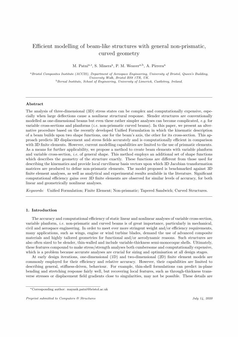
Figure 1: Unified Formulation framework - 3D structure discretisation.
conclusions are drawn in Section 5.
2. Mathematical Formulation
2.1. Preliminaries
Consider a 3D beam-like structure with arbitrary geometry, as shown in Figure 1. A system of localcurvilinear coordinates (r, s, t) is selected to describe the structure, such that the beam’s axis is defined tobe along the s-direction and its cross-section to lie in the rt-plane. The orientation of material points withinthe structure is determined by the direction cosines of the triad (r, s, t) with respect to the global Cartesiancoordinate system (x, y, z). Having established a coordinate system at the beginning of the formulation,the following maths has been cast in the global coordinate system. Since the derivation regarding thetransformation is a standard procedure, it has not been included in the present article but can be foundin [52].
For points in the structure’s interior, the three-dimensional displacement field, in the global Cartesiancoordinate system, is given by
U(x, y, z) = {u v w}> , (1)
and the displacement gradient vector Φ can be written as
Φ = {u,x u,y u,z v,x v,y v,z w,x w,y w,z}> , (2)
where, here and henceforth, a subscript preceded by a comma denotes differentiation.To account for large deformations, the Green-Lagrange strain vector E can be considered, which, in its
Virtual variations of equation (3) [53] are given by
δE = δ
{[H +
1
2A
]Φ
}= [H +A] δΦ. (4)
In the present work, the material is assumed to undergo deformation within the linear elastic range, andtherefore, Hooke’s law provides the constitutive relation
S = CE, (5)
where S = {Sxx Syy Szz Syz Sxz Sxy}> is the second Piola-Kirchhoff stress tensor and C is thetransformed material stiffness matrix expressed in the global Cartesian coordinate system,
C =
C11 C12 C13 C14 C15 C16
C22 C23 C24 C25 C26
C33 C34 C35 C36
C44 C45 C46
Symmetric C55 C56
C66
. (6)
The coefficients Cij relate to the elastic coefficients in material coordinates, Cij , via the transformationmatrixQ, whose elements are obtained from the direction cosines of the material coordinate system projectedonto the global (x, y, z) coordinate directions. Specifically,
C = QCQ>. (7)
The coefficients Cij and the matrixQ are not included here for sake of brevity, but can be found in Section 5.4of [54].
The Cauchy stress tensor σ is derived from the Second-Piola stress tensor S using the deformationgradient F . Specifically,
σ =1
detFFSF>, (8)
where
F =
1 + u,x u,y u,zv,x 1 + v,y v,zw,x w,y 1 + w,z
. (9)
The Cauchy stress tensor is referenced in the global coordinate system, which does not have a clear physicalmeaning in case of large deformations. Therefore, corotational Cauchy stresses are computed on the deformedconfiguration using the rotation tensor, R:
σ = R>σR. (10)
The rotation tensor R is obtained by polar decomposition of the deformation gradient as per [55].
5
st
r
Ni(y)
Fτ (x, z)
yz
x
Figure 2: Unified Formulation framework - 3D structure discretisation.
2.2. Serendipity-Lagrange-based Finite Element Model
Our model employs the Unified Formulation framework [31, 32], where a 3D beam-like structure isdiscretised with a finite number of transverse planes distributed along the principal axis. For simplicity, thisaxis can be thought of as the beam axis and the transverse planes as the beam cross-sections as shown inFigure 2. In order to maintain a consistent coordinate system throughout, the position of material pointsin the structure and all of the functions describing elasticity are expressed in global Cartesian coordinatesthrough a mapping of the type (x, y, z) = φ (r, s, t). This transformation between global and local coordinatescan be established either analytically or numerically.
The Unified Formulation relies on a displacement-based version of the finite element method. In thecurrent setting, the longitudinal axis of the structure is discretised with Ne-noded, 1D finite elements, sothat the displacement field can be approximated element-wise by means of local shape functions, Ni(y), andgeneralised nodal displacements, Ui(x, z), such that
U(x, y, z) =
Ne∑i=1
Ni(y)Ui(x, z). (11)
The transverse, or cross-sectional deformations, are approximated using hierarchical Serendipity Lagrangeexpansion (SLE) functions, Fτ (x, z) [51]. Adopting this expansion model, cross-sections are further discre-tised using four-noded Lagrange sub-domains (SLE nodes). The displacement field within each sub-domaincan be enriched by increasing the order of the local Serendipity Lagrange expansion. The cross-sectionaldisplacement field at the ith beam node is expressed as
Ui(x, z) =
m∑τ=1
Fτ (x, z)Uiτ , (12)
where m is the number of terms depending on the order of SL expansion, and Uiτ are generalized three-dimensional displacement vectors. The reader is referred to [37, 51] for a more detailed implementation andtreatment of SLE models.
By introducing the cross-sectional approximation of Eq. (12) into the FE discretisation along the beamaxis of Eq. (11), the displacement field reads
U(x, y, z) =
Ne∑i=1
m∑τ=1
Ni(y)Fτ (x, z)Uiτ . (13)
6
For the sake of clarity, it is important to emphasise that, using Eq. (13), the cross-sectional mesh (indicatedby discretisation variable τ) captures the warping of the cross-section with one set of 2D shape functions(Fτ (x, z)), while the axial behaviour is modelled by a separate 1D mesh (indicated by discretisation variable i)with an independent set of 1D shape functions (Ni(y)). This approach differentiates the method from classic3D FE models, where 3D shape functions are used over volumetric brick or tetrahedral elements that offerno separation of cross-sectional and axial deformations.
By substituting Eq. (13) in Eq. (2), the displacement gradient vector can be written as
In the previous expression and throughout the remainder of the paper, the Einstein summation conventionis indicated with repeated indices.
Elastic equilibrium is enforced via the Principle of Virtual Displacements, which in a quasi-static setting,states that
δWint = δWext, (15)
where Wint and Wext denote the internal and external work, respectively. By definition, the internal work isthe work done by the internal stresses over the corresponding internal strains and is equivalent to the elasticstrain energy. Noting that Wint =
∑eW
eint, where W e
int represents the strain energy per element and lettingV e be the volume of the generic element in an undeformed state,
δW eint =
∫V e
δE>S dV. (16)
In the notation of the Unified Formulation [51], the internal work can be re-written as
δW eint = δU>jsK
τsijs Uiτ , (17)
where the term Kτsijs is referred to as the Fundamental Nucleus of the secant stiffness matrix. Its explicit
form for an orthotropic lamina can be found in [56]. The main disadvantage of using the secant stiffnessmatrix is its low convergence rate when employed with the full Newton-Raphson method for solving thenonlinear governing equations. Moreover, the secant matrix is not uniquely defined and is generally non-symmetric. Therefore, we use the tangent stiffness matrix KT obtained from the linearisation of the virtualvariation of the strain energy,
d(δW eint) = δU>jsK
τsijT dUiτ . (18)
Fundamental nuclei are assembled into a global stiffness matrix following the standard finite element proce-dure. For the sake of brevity, the derivation and the explicit form of the fundamental nucleus of the tangentstiffness matrix is not reported here, but can be found in the authors’ recent work [35].
3. 3D Mapping via Jacobian Transformation
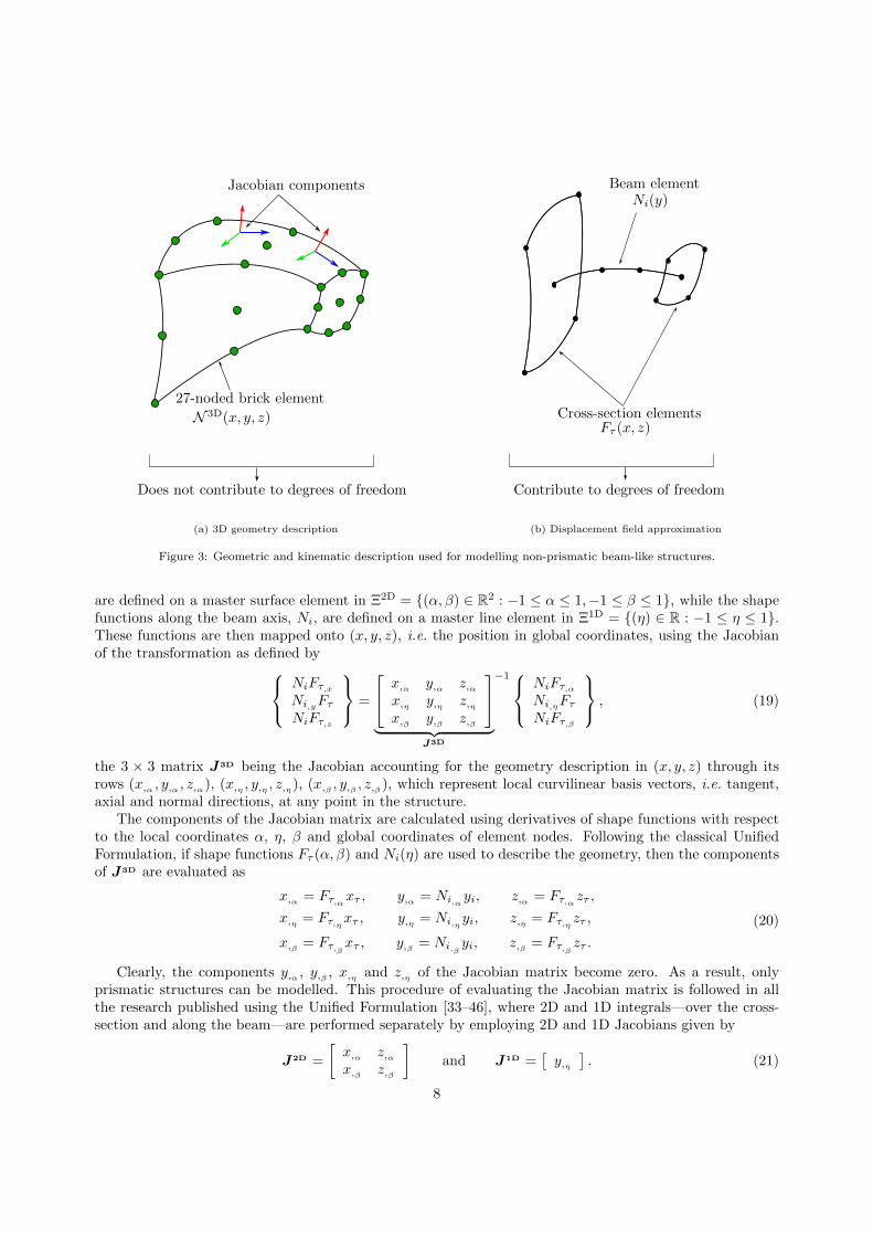
As discussed in Section 2.2, the Unified Formulation employs two shape functions, Fτ (x, z) and Ni(y),to describe the kinematics of the structure as given by Eq. (13). The cross-section expansion functions, Fτ ,
7
27-noded brick element
Jacobian components
Does not contribute to degrees of freedom
N 3D(x, y, z)
(a) 3D geometry description
Cross-section elements
Beam element
Contribute to degrees of freedom
Ni(y)
Fτ (x, z)
(b) Displacement field approximation
Figure 3: Geometric and kinematic description used for modelling non-prismatic beam-like structures.
are defined on a master surface element in Ξ2D = {(α, β) ∈ R2 : −1 ≤ α ≤ 1,−1 ≤ β ≤ 1}, while the shapefunctions along the beam axis, Ni, are defined on a master line element in Ξ1D = {(η) ∈ R : −1 ≤ η ≤ 1}.These functions are then mapped onto (x, y, z), i.e. the position in global coordinates, using the Jacobianof the transformation as defined by NiFτ,x
Ni,yFτNiFτ,z
=
x,α y,α z,αx,η y,η z,ηx,β y,β z,β
︸ ︷︷ ︸
J3D
−1 NiFτ,αNi,ηFτNiFτ,β
, (19)
the 3 × 3 matrix J3D being the Jacobian accounting for the geometry description in (x, y, z) through itsrows (x,α , y,α , z,α), (x,η , y,η , z,η ), (x,β , y,β , z,β ), which represent local curvilinear basis vectors, i.e. tangent,axial and normal directions, at any point in the structure.
The components of the Jacobian matrix are calculated using derivatives of shape functions with respectto the local coordinates α, η, β and global coordinates of element nodes. Following the classical UnifiedFormulation, if shape functions Fτ (α, β) and Ni(η) are used to describe the geometry, then the componentsof J3D are evaluated as
x,α = Fτ,αxτ , y,α = Ni,α yi, z,α = Fτ,α zτ ,
x,η = Fτ,ηxτ , y,η = Ni,η yi, z,η = Fτ,η zτ ,
x,β = Fτ,β xτ , y,β = Ni,β yi, z,β = Fτ,β zτ .
(20)
Clearly, the components y,α , y,β , x,η and z,η of the Jacobian matrix become zero. As a result, onlyprismatic structures can be modelled. This procedure of evaluating the Jacobian matrix is followed in allthe research published using the Unified Formulation [33–46], where 2D and 1D integrals—over the cross-section and along the beam—are performed separately by employing 2D and 1D Jacobians given by
J2D =
[x,α z,αx,β z,β
]and J1D =
[y,η
]. (21)
8
To overcome the above limitation and to model general beam-like structures (e.g. non-prismatic, curvedbeams), we propose to use an additional set of functions to represent the element geometry. These couldbe CAD basis functions, such as B-splines or Non-Uniform Rational B-Splines (NURBS), that guaranteean exact geometric representation or could be higher-order Lagrange functions. On the other hand, theUnified Formulation functions Fτ and Ni are used, in the usual manner, for approximating the displacementfield. To demonstrate the validity of the proposed technique, in the present work, we discretise structuralgeometry using 27-noded brick elements, with 3D Lagrange shape functions, N 3D(x, y, z), to evaluate localcurvilinear basis vectors (or Jacobian matrix components) at each point, as shown in Figure 3. Followingthis procedure, the components of J3D are evaluated as
x,α = N 3D,α xτ , y,α = N 3D
,α yi, z,α = N 3D,α zτ ,
x,η = N 3D,η xτ , y,η = N 3D
,η yi, z,η = N 3D,η zτ ,
x,β = N 3D,βxτ , y,β = N 3D
,βyi, z,β = N 3D
,βzτ .
(22)
Furthermore, it is important to note that, the proposed methodology requires integration along the beamaxis and over the cross-section to be performed simultaneously. For instance, the first component of thefundamental nucleus of the tangent stiffness matrix (for a geometrically linear model) is given as follows [35]:
KτsijT (1, 1) =
∫V
C11Fτ,xFs,xNiNjdV +
∫V
C16Fτ,xFsNiNj,ydV +
∫V
C15Fτ,xFs,zNiNjdV
+
∫V
C16FτFs,xNi,yNjdV +
∫V
C66FτFsNi,yNj,ydV +
∫V
C56FτFs,zNi,yNjdV
+
∫V
C15Fτ,zFs,xNiNjdV +
∫V
C56Fτ,zFsNiNj,ydV +
∫V
C55Fτ,zFs,zNiNjdV.
(23)
The integrals are evaluated numerically by employing Gaussian Quadrature. The first term of Eq. (23) canbe evaluated as∫
V
C11Fτ,xFs,xNiNjdV =
∫ 1
−1
∫ 1
−1
∫ 1
−1
C11
(NiFτ,x
)(NjFs,x
)|J3D |dα dη dβ
=
lgp∑l=1
kgp∑k=1
mgp∑m=1
C11(αl, ηk, βm)(Ni(ηk)Fτ,x(αl, βm)
)(Nj(ηk)Fs,x(αl, βm)
)|J3D |wlwkwm,
(24)
where: wl, wk and wm are the weights related to the Gauss points αl, ηk and βm; lgp, kgp and mgp are thenumber of Gauss points used; C11(αl, ηk, βm) is the material constant evaluated at a specific Gauss point;|J3D | is the determinant of the Jacobian matrix.
In contrast, the classical Unified Formulation approach splits the beam and the cross-sectional integrationas follows: ∫
V
C11Fτ,xFs,xNiNjdV = C11
∫ 1
−1
∫ 1
−1
Fτ,xFs,x |J2D |dα dβ∫ 1
−1
NiNj |J1D |dη
= C11
lgp∑l=1
mgp∑m=1
Fτ,x(αl, βm)Fs,x(αl, βm)|J2D |wlwmkgp∑k=1
Ni(ηk)Nj(ηk)|J1D |wk.(25)
Clearly, Eq. (24) is computationally more expensive to evaluate than Eq. (25), as the number of loopsrequired increases from (lgp ×mgp + kgp) to (lgp × kgp ×mgp). Nevertheless, by performing the beam andthe cross-sectional integration simultaneously and also by considering the 3D Jacobian matrix, enhances theUnified Formulation modelling capabilities.
9
Table 1: Dimensions of the tapered I-beam (in mm).
Web width bw = 6 Web height hw(0) = 900 Web height hw(L) = 100
y
z
V (L)
L
hw(y)
M(L)
M(0)
V (0)
z
x
bw
bf
hf
hf
bf
Figure 4: Tapered I-section beam: dimensions and load definition.
4. Numerical Results
In this section, the proposed UF-SLE model is assessed by means of static analyses of various non-prismatic and curved structures. The first example concerns a tapered I-beam. Then, a tapered sandwichbeam-like structure is considered and the effect of increasing taper angle on the 3D stress distributionis studied. Finally, three corrugated structures of different depth are considered. The relative nonlinearforce-displacement and stress responses are compared with numerical and experimental results.
4.1. Tapered I-beam
The tapered I-beam analysed here is shown in Figure 4. Its dimensions are shown in Table 1. TheYoung’s modulus, E, and Poisson’s ratio, ν, of the constituent material are 210 GPa and 0.3, respectively.The forces and moments acting on the beam ends are
V (0) = 100 kN, M(0) = 700 kNm.
V (L) = 100 kN, M(L) = 300 kNm.
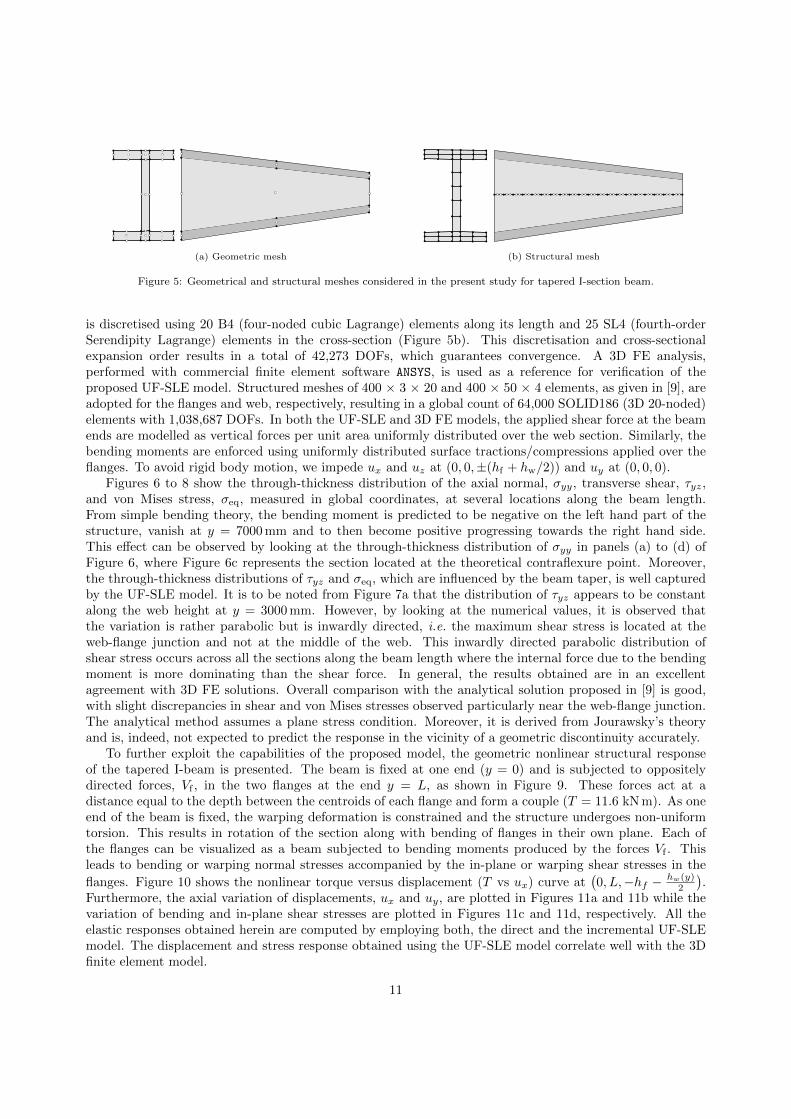
The example is adapted from [9], which employs a planar non-prismatic beam model [8] with enhancedstress recovery, based on a rigorous generalisation of Jourawsky’s theory. Solving this problem with theUF-SLE model requires two input meshes as shown in Figure 5. The first mesh consists of 27-noded brickelements used to discretise the structure’s geometry. Using this data and employing 3D Lagrange shapefunctions, local basis vectors representing the orientation of each structural component (web and flanges)can be computed at the grid nodes. The number of elements used to discretise the structure should becarefully chosen to ensure that the geometry is represented to the desired level of accuracy. Seven elementsare sufficient in this case as shown in Figure 5a. These geometric elements contribute marginally in termsof computational cost as they do not contribute to the total structural degrees of freedom (DOFs). Thesecond mesh is structural and contains the nodes of the Unified Formulation finite element discretisation, i.e.the nodes defining cross-sectional computational domains [51] and 1D beam elements. This I-section beam
10
(a) Geometric mesh (b) Structural mesh
Figure 5: Geometrical and structural meshes considered in the present study for tapered I-section beam.
is discretised using 20 B4 (four-noded cubic Lagrange) elements along its length and 25 SL4 (fourth-orderSerendipity Lagrange) elements in the cross-section (Figure 5b). This discretisation and cross-sectionalexpansion order results in a total of 42,273 DOFs, which guarantees convergence. A 3D FE analysis,performed with commercial finite element software ANSYS, is used as a reference for verification of theproposed UF-SLE model. Structured meshes of 400 × 3 × 20 and 400 × 50 × 4 elements, as given in [9], areadopted for the flanges and web, respectively, resulting in a global count of 64,000 SOLID186 (3D 20-noded)elements with 1,038,687 DOFs. In both the UF-SLE and 3D FE models, the applied shear force at the beamends are modelled as vertical forces per unit area uniformly distributed over the web section. Similarly, thebending moments are enforced using uniformly distributed surface tractions/compressions applied over theflanges. To avoid rigid body motion, we impede ux and uz at (0, 0,±(hf + hw/2)) and uy at (0, 0, 0).
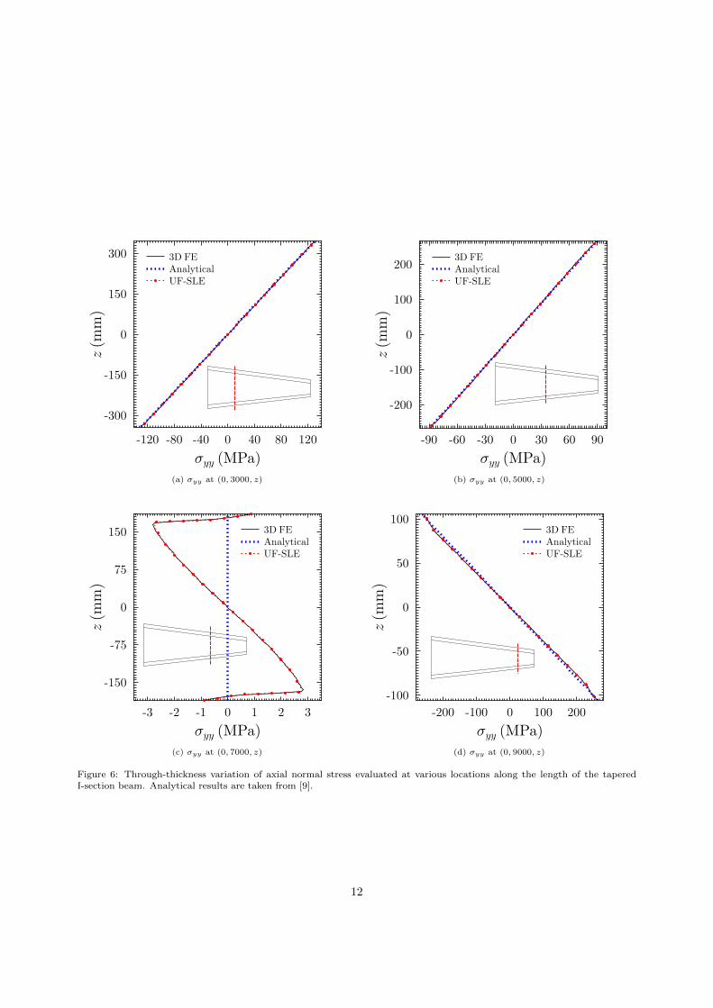
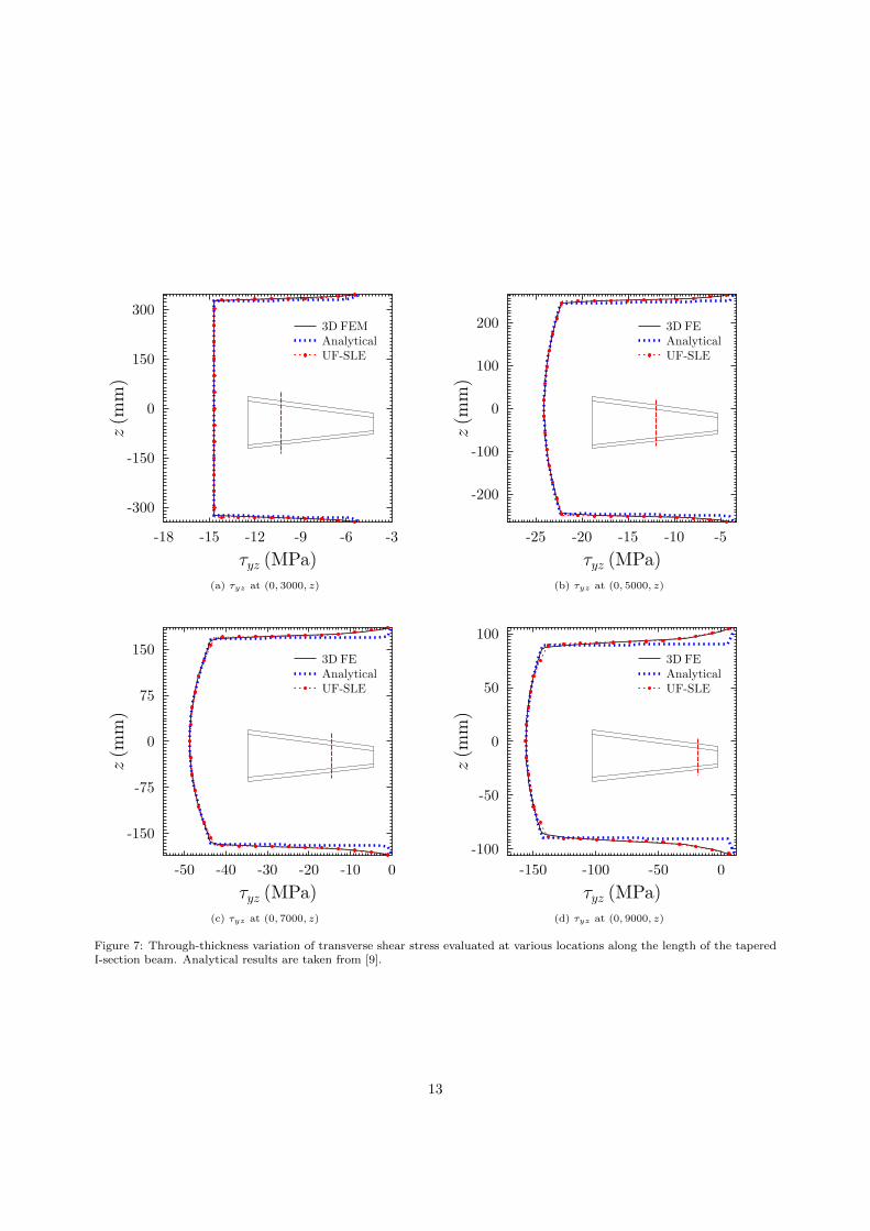
Figures 6 to 8 show the through-thickness distribution of the axial normal, σyy, transverse shear, τyz,and von Mises stress, σeq, measured in global coordinates, at several locations along the beam length.From simple bending theory, the bending moment is predicted to be negative on the left hand part of thestructure, vanish at y = 7000 mm and to then become positive progressing towards the right hand side.This effect can be observed by looking at the through-thickness distribution of σyy in panels (a) to (d) ofFigure 6, where Figure 6c represents the section located at the theoretical contraflexure point. Moreover,the through-thickness distributions of τyz and σeq, which are influenced by the beam taper, is well capturedby the UF-SLE model. It is to be noted from Figure 7a that the distribution of τyz appears to be constantalong the web height at y = 3000 mm. However, by looking at the numerical values, it is observed thatthe variation is rather parabolic but is inwardly directed, i.e. the maximum shear stress is located at theweb-flange junction and not at the middle of the web. This inwardly directed parabolic distribution ofshear stress occurs across all the sections along the beam length where the internal force due to the bendingmoment is more dominating than the shear force. In general, the results obtained are in an excellentagreement with 3D FE solutions. Overall comparison with the analytical solution proposed in [9] is good,with slight discrepancies in shear and von Mises stresses observed particularly near the web-flange junction.The analytical method assumes a plane stress condition. Moreover, it is derived from Jourawsky’s theoryand is, indeed, not expected to predict the response in the vicinity of a geometric discontinuity accurately.
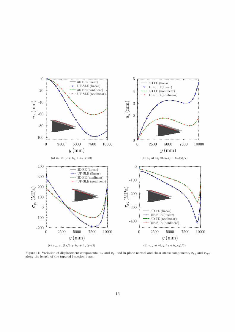
To further exploit the capabilities of the proposed model, the geometric nonlinear structural responseof the tapered I-beam is presented. The beam is fixed at one end (y = 0) and is subjected to oppositelydirected forces, Vf , in the two flanges at the end y = L, as shown in Figure 9. These forces act at adistance equal to the depth between the centroids of each flange and form a couple (T = 11.6 kN m). As oneend of the beam is fixed, the warping deformation is constrained and the structure undergoes non-uniformtorsion. This results in rotation of the section along with bending of flanges in their own plane. Each ofthe flanges can be visualized as a beam subjected to bending moments produced by the forces Vf . Thisleads to bending or warping normal stresses accompanied by the in-plane or warping shear stresses in the
flanges. Figure 10 shows the nonlinear torque versus displacement (T vs ux) curve at(0, L,−hf − hw(y)
2
).
Furthermore, the axial variation of displacements, ux and uy, are plotted in Figures 11a and 11b while thevariation of bending and in-plane shear stresses are plotted in Figures 11c and 11d, respectively. All theelastic responses obtained herein are computed by employing both, the direct and the incremental UF-SLEmodel. The displacement and stress response obtained using the UF-SLE model correlate well with the 3Dfinite element model.
11
(a) σyy at (0, 3000, z) (b) σyy at (0, 5000, z)
(c) σyy at (0, 7000, z) (d) σyy at (0, 9000, z)
Figure 6: Through-thickness variation of axial normal stress evaluated at various locations along the length of the taperedI-section beam. Analytical results are taken from [9].
12
(a) τyz at (0, 3000, z) (b) τyz at (0, 5000, z)
(c) τyz at (0, 7000, z) (d) τyz at (0, 9000, z)
Figure 7: Through-thickness variation of transverse shear stress evaluated at various locations along the length of the taperedI-section beam. Analytical results are taken from [9].
13
(a) σeq at (0, 3000, z) (b) σeq at (0, 5000, z)
(c) σeq at (0, 7000, z) (d) σeq at (0, 9000, z)
Figure 8: Through-thickness variation of von Mises stress evaluated at various locations along the length of the tapered I-sectionbeam. Analytical results are taken from [9].
14
y
z
z
x
Vf
Vf
Vf = 100kN
Figure 9: Tapered I-section beam: under twisting load.
Figure 10: Tapered I-section beam: Applied twisting moment versus lateral displacement curve at(0, L,−hf − hw(y)
2
).
15
(a) ux at (0, y, hf + hw(y)/2) (b) uy at (bf/2, y, hf + hw(y)/2)
(c) σyy at (bf/2, y, hf + hw(y)/2) (d) τxy at (0, y, hf + hw(y)/2)
Figure 11: Variation of displacement components, ux and uy , and in-plane normal and shear stress components, σyy and τxy ,along the length of the tapered I-section beam.
16
y
z
φ
Pz
L
hc(y)
hf
z
x
b
hc(0)
s
n
s
n
hf
Figure 12: Tapered sandwich beam: dimensions and load definition.
Table 2: Mechanical properties of the IM7/8552 graphite-epoxy composite [57].
E1 E2 E3 G13 G23 G12 ν13 ν23 ν12
(GPa)
150 9.08 9.08 5.6 2.8 5.6 0.32 0.5 0.32
4.2. Tapered Sandwich Beam-like 3D Structure
In this section, a tapered sandwich beam-like structure of length L = 1000 mm and width b = 300 mmis considered, as shown in Figure 12. The beam is fixed at y = 0 and subjected to a transverse force, Pz,applied as a uniformly distributed load across the section at y = L. The facings of the sandwich compositeare made of IM7/8552 graphite-epoxy material of thickness hf = 10 mm. Material properties in principalmaterial coordinates are shown in Table 2. The core is assumed to be made of PVC foam with isotropicproperties: Young’s modulus, E = 100 MPa and shear modulus, G = 38.5 MPa. The core’s thickness varieslinearly along the beam length, starting from hc(0) = 300 mm and ending at different values depending onthe taper angle, φ.
Using the UF-SLE model, the beam is discretised with 20 B4 elements along its length. The nodesare distributed adopting a Chebyshev biased mesh. This distribution in the longitudinal direction capturesboundary layer effects induced by the clamped support accurately [51]. The initial cross-section (at y = 0)is discretised with 3 SL5 (fifth-order Serendipity Lagrange) elements with one element for each outer facingand one for the core. This discretisation and order of expansion results in 10,431 DOFs. In addition,
(a) Geometric mesh (b) Structural mesh
Figure 13: Geometrical and structural meshes considered in the present study for tapered sandwich beam.
17
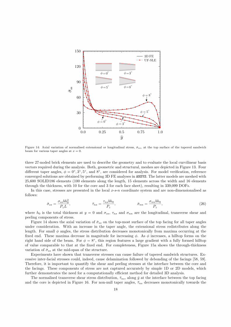
Figure 14: Axial variation of normalised extensional or longitudinal stress, σss, at the top surface of the tapered sandwichbeam for various taper angles at x = 0.
three 27-noded brick elements are used to describe the geometry and to evaluate the local curvilinear basisvectors required during the analysis. Both, geometric and structural, meshes are depicted in Figure 13. Fourdifferent taper angles, φ = 0◦, 3◦, 5◦, and 8◦, are considered for analysis. For model verification, referenceconverged solutions are obtained by performing 3D FE analyses in ANSYS. The latter models are meshed with25,600 SOLID186 elements (100 elements along the length, 15 elements across the width and 16 elementsthrough the thickness, with 10 for the core and 3 for each face sheet), resulting in 339,099 DOFs.
In this case, stresses are presented in the local x-s-n coordinate system and are non-dimensionalised asfollows:
σss =σssbh
20
PzL, τns =
τnsbh0
Pz, σnn =
σnnbh0
Pz, (26)
where h0 is the total thickness at y = 0 and σss, τns and σnn are the longitudinal, transverse shear andpeeling components of stress.
Figure 14 shows the axial variation of σss on the top-most surface of the top facing for all taper anglesunder consideration. With an increase in the taper angle, the extensional stress redistributes along thelength. For small φ angles, the stress distribution decreases monotonically from maxima occurring at thefixed end. These maxima decrease in magnitude for increasing φ. As φ increases, a hilltop forms on theright hand side of the beam. For φ = 8◦, this region features a large gradient with a fully formed hilltopof value comparable to that at the fixed end. For completeness, Figure 15a shows the through-thicknessvariation of σss at the mid-span of the structure.
Experiments have shown that transverse stresses can cause failure of tapered sandwich structures. Ex-cessive inter-facial stresses could, indeed, cause delamination followed by debonding of the facings [58, 59].Therefore, it is important to quantify the shear and peeling stresses at the interface between the core andthe facings. These components of stress are not captured accurately by simple 1D or 2D models, whichfurther demonstrates the need for a computationally efficient method for detailed 3D analysis.
The normalised transverse shear stress distribution, τns, along y at the interface between the top facingand the core is depicted in Figure 16. For non-null taper angles, τns decreases monotonically towards the
18
(a) σss at (0, L/2, z) (b) τns at (0, L/2, z)
Figure 15: Through-thickness distribution of normalised extensional and normalised transverse shear stress at the mid-span ofthe tapered sandwich beam for various taper angles obtained by the UF-SLE model.
free end, featuring sharp gradients towards both ends and reaching greater maximum absolute values forincreasing angles. This contrasts with the observation that, at the mid-span of the beam, transverse shearstresses decrease as the taper angle increases, as shown in Figure 15b. For the prismatic case, the transverseshear stress is nearly constant, except in the vicinity of the clamped end, where the sharp gradient ismaintained, and at the free end where a concentrated local minimum is observed.
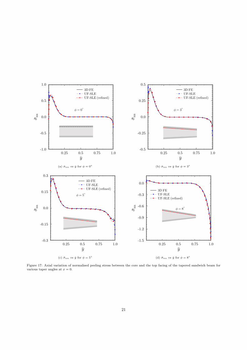
Finally, Figure 17 shows the axial variation of normalised peeling stress, σnn, between the core and thetop facing. Compared to 3D FE solutions, adopting the same mesh as for the other two components ofstress, small discrepancies are observed near the ends. Therefore, σnn is further investigated by using arefined mesh (40 B4 Chebyshev-biased beam elements and 9 SL5 elements in the cross-section: one per layerand three across the width). The peeling stress response obtained using the refined mesh correlates wellwith 3D FE solutions. Although, slight differences are still noticed near the ends, which are predominantlyin the first and the last beam elements. The reason for this discrepancy could be the different order ofexpansions used in the cross-section and in the beam direction, which are quintic and cubic, respectively.The issue could be addressed by adopting higher-order beam elements. However, solving this disparity inresults near the constraints, needs further investigation and will be explored in future work.
It is observed that, for all cases, peak stress values localise towards the ends and are negligible everywhereelse. The large peeling stress near the ends could cause the facing to peel off from the core. The overall 3Dstress response in the tapered sandwich structures is well predicted by the proposed UF-SLE model and iscomputationally efficient compared to the 3D FE model.
4.3. Corrugated Structures
In order to further exploit the capabilities of the UF-SLE model, the geometric nonlinear behaviour ofcorrugated structures in tensile loading is investigated. This example is adapted from the work done byThurnherr et al. [60]. The objective is to show the proposed model’s capability in analysing such complexcurved structures and describing their nonlinear behaviour.
A corrugation pattern consisting of unit cells with circular sections is now described. The elementary unitcell is shown in Figure 18, together with the definition of its parameters: radius of curvature, R; amplitude,c; periodic cell length, p; arc-length parameter, s; and coordinates (y(s), z(s)) of points on the mid-surface.
19
(a) τns vs y for φ = 0◦ (b) τns vs y for φ = 3◦
(c) τns vs y for φ = 5◦ (d) τns vs y for φ = 8◦
Figure 16: Axial variation of normalised transverse shear stress between the core and the top facing of the tapered sandwichbeam for various taper angles at at x = 0.
20
(a) σnn vs y for φ = 0◦ (b) σnn vs y for φ = 3◦
(c) σnn vs y for φ = 5◦ (d) σnn vs y for φ = 8◦
Figure 17: Axial variation of normalised peeling stress between the core and the top facing of the tapered sandwich beam forvarious taper angles at x = 0.
21
z
y
s
cR
p
(y(s), z(s))
Figure 18: Corrugated structure: unit cell geometry definition.
The latter are given by the parametric equations [61, 62]:
y(s) = R [sinψ(s) + (2 +m) sinψ0] ,
z(s) = −mR [cosψ(s)− cosψ0] ,(27)
where
m =
{1 if y ≤ p/2−1 if y > p/2
, (28)
ψ0 =
{arcsin
(p
4R
)if c ≤ p
4arccos
(p
4R
)+ π
2 if c > p4
, (29)
representing the opening angle indicated in Figure 18, and
ψ(s) = κs− (2−m)ψ0. (30)
Finally, the radius of curvature, R, follows from p and c, and is given by
R =16c2 + p2
32c. (31)
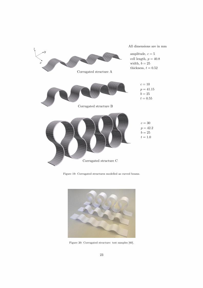
Three different structures, referred to as A, B and C, and each consisting of four unit cells, are studied.The dimensions for each case are shown in Figure 19. All configurations are clamped on both sides with anaxial displacement, uy, applied on one end. Thurnherr et al. [60] conducted an experimental study on thesestructures. The test samples shown in Figure 20 were fabricated using a 3D printer. All specimens weremade from Polylactic acid (PLA). Due to the fabrication process the samples are printed layer by layer. Thisleads to anisotropic material behaviour where the direction parallel to the layers is the stiffest. However,under tensile loading the mechanical response is mainly governed by the stiffness in the axial direction.Therefore, the constituent material is assumed to be isotropic [60] with Young’s modulus E = 3.5 GPa andPoisson’s ratio ν = 0.346.
Herein, the corrugated structures are analysed using the UF-SLE model. Configuration A is discretisedwith three SL3 (third-order expansion) elements in the cross-section and 50 B4 elements along the longitu-dinal direction. An increase in curvature demands a finer discretisation to capture nonlinear deflection andstress accurately. Hence, specimens B and C require respectively 80 and 150 B4 elements. These discretisa-tions result in 12,684, 20,224 and 37,884 DOFs for configurations A, B and C, respectively. In order to verifythe results obtained using the UF-SLE model, 3D FE analyses are performed using ANSYS. In all cases,the structures are discretised using 13,440 SOLID186 (20-noded brick) elements (with 2 elements throughthe thickness, 320 elements along the corrugation pattern and 20 elements across the width), resulting in229,959 DOFs. It is to be noted that a third-order SLE model is employed in the cross-section, resulting
22
amplitude, c = 5
cell length, p = 40.8
width, b = 25
thickness, t = 0.52
c = 10
p = 41.15
b = 25
t = 0.55
c = 30
p = 42.2
b = 25
t = 1.0
Corrugated structure A
Corrugated structure B
Corrugated structure C
zy
x
All dimensions are in mm
Figure 19: Corrugated structures modelled as curved beams.
Figure 20: Corrugated structure: test samples [60].
23
in a highly refined kinematic field, which may not be required for a thin structure under tensile load. Also,solid elements are employed in the FE analysis where shell elements could have been used instead. Thisexpansion order and the type of finite element are used to ensure minimum error in the solutions. Moreover,the objective of this test case is to showcase the validity of the proposed model in analysing highly curvedstructures, and not to compare the computational efficiencies of the two approaches.
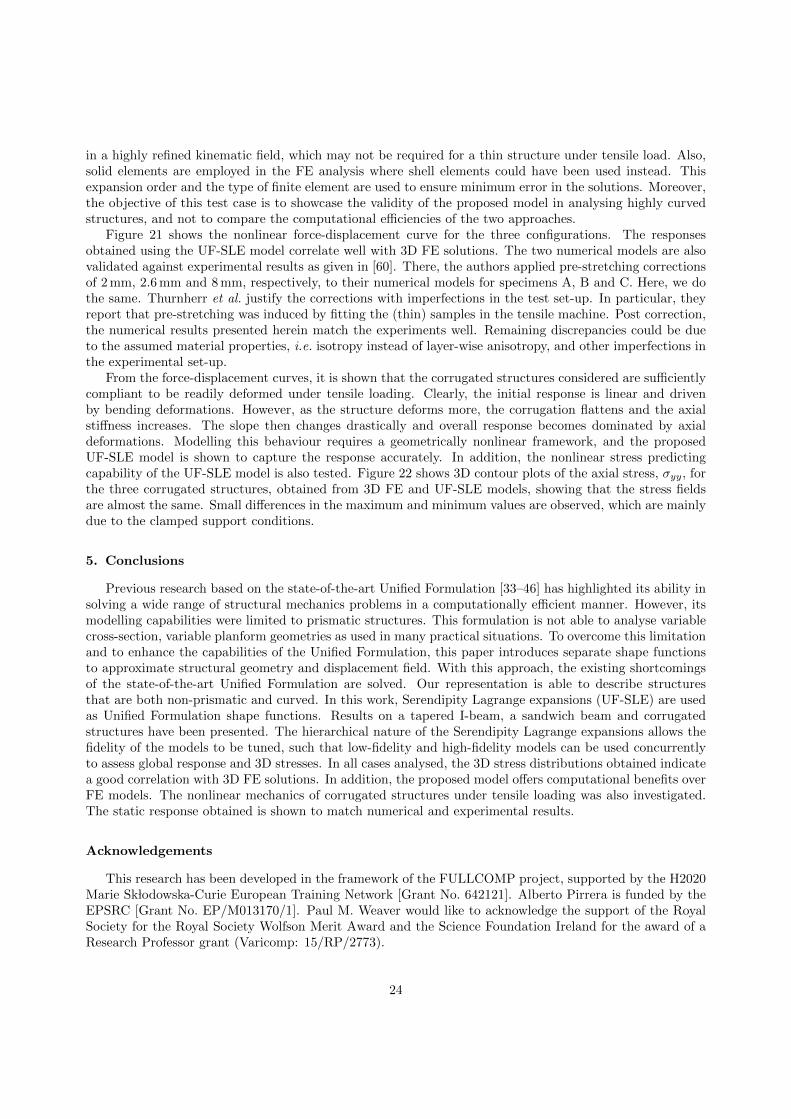
Figure 21 shows the nonlinear force-displacement curve for the three configurations. The responsesobtained using the UF-SLE model correlate well with 3D FE solutions. The two numerical models are alsovalidated against experimental results as given in [60]. There, the authors applied pre-stretching correctionsof 2 mm, 2.6 mm and 8 mm, respectively, to their numerical models for specimens A, B and C. Here, we dothe same. Thurnherr et al. justify the corrections with imperfections in the test set-up. In particular, theyreport that pre-stretching was induced by fitting the (thin) samples in the tensile machine. Post correction,the numerical results presented herein match the experiments well. Remaining discrepancies could be dueto the assumed material properties, i.e. isotropy instead of layer-wise anisotropy, and other imperfections inthe experimental set-up.
From the force-displacement curves, it is shown that the corrugated structures considered are sufficientlycompliant to be readily deformed under tensile loading. Clearly, the initial response is linear and drivenby bending deformations. However, as the structure deforms more, the corrugation flattens and the axialstiffness increases. The slope then changes drastically and overall response becomes dominated by axialdeformations. Modelling this behaviour requires a geometrically nonlinear framework, and the proposedUF-SLE model is shown to capture the response accurately. In addition, the nonlinear stress predictingcapability of the UF-SLE model is also tested. Figure 22 shows 3D contour plots of the axial stress, σyy, forthe three corrugated structures, obtained from 3D FE and UF-SLE models, showing that the stress fieldsare almost the same. Small differences in the maximum and minimum values are observed, which are mainlydue to the clamped support conditions.
5. Conclusions
Previous research based on the state-of-the-art Unified Formulation [33–46] has highlighted its ability insolving a wide range of structural mechanics problems in a computationally efficient manner. However, itsmodelling capabilities were limited to prismatic structures. This formulation is not able to analyse variablecross-section, variable planform geometries as used in many practical situations. To overcome this limitationand to enhance the capabilities of the Unified Formulation, this paper introduces separate shape functionsto approximate structural geometry and displacement field. With this approach, the existing shortcomingsof the state-of-the-art Unified Formulation are solved. Our representation is able to describe structuresthat are both non-prismatic and curved. In this work, Serendipity Lagrange expansions (UF-SLE) are usedas Unified Formulation shape functions. Results on a tapered I-beam, a sandwich beam and corrugatedstructures have been presented. The hierarchical nature of the Serendipity Lagrange expansions allows thefidelity of the models to be tuned, such that low-fidelity and high-fidelity models can be used concurrentlyto assess global response and 3D stresses. In all cases analysed, the 3D stress distributions obtained indicatea good correlation with 3D FE solutions. In addition, the proposed model offers computational benefits overFE models. The nonlinear mechanics of corrugated structures under tensile loading was also investigated.The static response obtained is shown to match numerical and experimental results.
Acknowledgements
This research has been developed in the framework of the FULLCOMP project, supported by the H2020Marie Sk lodowska-Curie European Training Network [Grant No. 642121]. Alberto Pirrera is funded by theEPSRC [Grant No. EP/M013170/1]. Paul M. Weaver would like to acknowledge the support of the RoyalSociety for the Royal Society Wolfson Merit Award and the Science Foundation Ireland for the award of aResearch Professor grant (Varicomp: 15/RP/2773).
24
(a) Corrugated Structure A. (b) Corrugated Structure B.
(c) Corrugated Structure C.
Figure 21: Force vs axial displacement curve for the three corrugated structures A, B and C. Experimental results are takenfrom Thurnherr et al. [60].
25
UF-SLE3D FE
-54.8 -16.3 22.2 60.7 99.2 138
Corrugated Structure A
-82.8 -26.8 29.1 85.1 141 197
3D FE UF-SLE
Corrugated Structure B
-138 79.2 -20.4 38.4 97.2 156
3D FE UF-SLE
Corrugated Structure C
-55.6 -16.2 23.2 62.5 102 141
-77.2 -19.9 37.3 94.6 152 209
-146 -82 -18.3 45.4 109 173
Figure 22: Contour plot of axial normal stress σyy (in Pa) for the three corrugated structures A, B and C.
26
Data Statement
All data required to reproduce the figures in this paper can be found on the data repository of theUniversity of Bristol via URL: http://data.bris.ac.uk/data/.
References
[1] L. S. Johansen, E. Lund, J. Kleist, Failure optimization of geometrically linear/nonlinear laminated composite structuresusing a two-step hierarchical model adaptivity, Computer Methods in Applied Mechanics and Engineering 198 (2009)2421–2438.
[2] B. Kim, A. Oliver, J. Vyse, Bending Stresses of Steel Web Tapered Tee Section Cantilevers, Journal of Civil Engineeringand Architecture 7 (11) (2013) 1329–1342.
[3] A. Beltempo, G. Balduzzi, G. Alfano, F. Auricchio, Analytical derivation of a general 2D non-prismatic beam model basedon the Hellinger-Reissner principle, Engineering Structures 101 (2015) 88–98.
[4] G. Balduzzi, M. Aminbaghai, E. Sacco, J. Fussl, J. Eberhardsteiner, F. Auricchio, Non-prismatic beams: a simple andeffective Timoshenko-like model, International Journal of Solids and Structures 90 (2016) 236–250.
[5] V. Mercuri, G. Balduzzi, D. Asprone, F. Auricchio, 2D non-prismatic beam model for stiffness matrix evaluation, InProceedings of the Word Conference on Timber Engineering, 22-25 August 2016.
[6] D. H. Hodges, A. Rajagopal, J. C. Ho, W. Yu, Stress and strain recovery for the in-plane deformation of an isotropictapered strip-beam, Journal of Mechanics of Materials and Structures 5 (2010) 963–975.
[7] T. H. Trinh, B. S. Gan, Development of consistent shape functions for linearly solid tapered timoshenko beam, Journal ofStructural and Construction Engineering 80 (2015) 1103–1111.
[8] G. Balduzzi, M. Aminbaghai, E. Sacco, J. Fussl, Planar Timoshenko-like model for multilayer non-prismatic beams,International Journal of Mechanics and Materials in Design 14 (2018) 51–70.
[9] G. Balduzzi, G. Hochreiner, J. Fussl, Stress recovery from one dimensional models for tapered bi-symmetric thin-walledI beams: Deficiencies in modern engineering tools and procedures, Thin-Walled Structures journal 119 (2017) 934–945.
[10] A. P. Gupta, K. P. Sharma, Bending of a Sandwich Annular Plate of Variable Thickness, Indian Journal of Pure andApplied Mathematics 13 (1982) 1313–1321.
[11] N. Paydar, C. Libove, Stress Analysis of Sandwich Plates of Variable Thickness, Journal of Applied Mechanics 55 (1988)419–424.
[12] C. Libove, C. H. Lu, Beamlike Bending of Variable-thickness Sandwich Plates, AIA Journal 12 (1989) 1617–1618.[13] C. H. Lu, Bending of Anisotropic Sandwich Beams with Variable Thickness, Journal of Thermoplastic Composite Materials
7 (1994) 364–374.[14] D. Peled, Y. Frostig, High-order Bending of Sandwich Beams with Variable Flexible Core and Nonparallel Skins, ASCE
Journal of Engineering Mechanics 120 (1994) 1255–1269.[15] S. V. Hoa, B. L. Du, T. Vu-Khanh, Interlaminar stresses in tapered laminates, Polymer Composites 9 (1988) 337–344.[16] J. S. Jeon, C. S. Hong, Bending of tapered anisotropic sandwich plates with arbitrary edge conditions, AIAA Journal 30
(1992) 1762–1769.[17] Q. Ai, P. M. Weaver, Simplified analytical model for tapered sandwich beams using variable stiffness materials, Journal
of Sandwich Structures and Materials 19 (2017) 3–25.[18] T. Belytschko, L. W. Glaum, Applications of higher order corotational stretch theories to nonlinear finite element analysis,
Computers & Structures 10 (1-2) (1979) 175–182.[19] L. W. Glaum, Direct Iteration and Perturbation Methods for the Analysis of Nonlinear Structures, Ph.D. thesis, University
of Illinois at Chicago (1976).[20] K. S. Surana, R. M. Sorem, Geometrically non-linear formulation for three dimensional curved beam elements with large
rotations, International Journal for Numerical Methods in Engineering 28 (1) (1989) 43–73.[21] A. Ibrahimbegovic, On finite element implementation of geometrically nonlinear reissner’s beam theory: three-dimensional
curved beam elements, Computer methods in applied mechanics and engineering 122 (1-2) (1995) 11–26.[22] A. Ibrahimbegovic, F. Frey, Finite element analysis of linear and non-linear planar deformations of elastic initially curved
beams, International Journal for Numerical Methods in Engineering 36 (19) (1993) 3239–3258.[23] A. Shahba, R. Attarnejad, M. Eslaminia, Derivation of an efficient non-prismatic thin curved beam element using basic
displacement functions, Shock and Vibration 19 (2012) 187–204.[24] R. Attarnejad, A. Shahba, S. J. Semnani, Analysis of Non-Prismatic Timoshenko Beams Using Basic Displacement
Functions, Advances in Structural Engineering 14 (2011) 319–332.[25] E. Petrov, M. Geradin, Finite element theory for curved and twisted beams based on exact solutions for three-dimensional
solids part 1: Beam concept and geometrically exact nonlinear formulation, Computer methods in applied mechanics andengineering 165 (1-4) (1998) 43–92.
[26] A. M. Yu, J. W. Yang, G. H. Nie, X. G. Yang, An improved model for naturally curved and twisted composite beamswith closed thin-walled sections, Composite Structures 93 (9) (2011) 2322–2329.
[27] C. N. Chen, DQEM analysis of in-plane vibration of curved beam structures, Advances in Engineering Software 36 (6)(2005) 412–424.
[28] G. Karami, P. Malekzadeh, In-plane free vibration analysis of circular arches with varying cross-sections using differentialquadrature method, Journal of Sound and Vibration 274 (2004) 777–799.
27
[29] M. A. D. Rosa, C. Franciosi, Exact and approximate analysis of circular arches using DQM, International Journal of Solidsand Structures 37 (2000) 1103–1117.
[30] S. Ghuku, K. N. Saha, A review on stress and deformation analysis of curved beams under large deflection, InternationalJournal of Engineering and Technology 11 (2017) 13–39.
[31] E. Carrera, M. Cinefra, M. Petrolo, E. Zappino, Finite Element Analysis of Structures through Unified Formulation, Wiley,Politecnico di Torino, Italy, 2014.
[32] E. Carrera, G. Giunta, M. Petrolo, A Modern and Compact Way to Formulate Classical and Advanced Beam Theories,Saxe-Coburg Publications, United Kingdom, 2010.
[33] E. Carrera, G. Giunta, P. Nali, M. Petrolo, Refined beam elements with arbitrary cross-section geometries, Computers &Structures 88 (2010) 283–293.
[34] E. Carrera, E. Zappino, One-dimensional finite element formulation with node-dependent kinematics, Computers & Struc-tures 192 (2017) 114–125.
[35] M. Patni, S. Minera, C. Bisagni, P. M. Weaver, A. Pirrera, Geometrically nonlinear finite element model for predictingfailure in composite structures, Composite Structures 225. doi:10.1016/j.compstruct.2019.111068.
[36] M. Petrolo, M. Nagaraj, I. Kaleel, E. Carrera, A global-local approach for the elastoplastic analysis of compact andthin-walled structures via refined models, Computers & Structures 206 (2018) 54–65.
[37] M. Patni, S. Minera, R. M. J. Groh, A. Pirrera, P. M. Weaver, Three-dimensional stress analysis for laminated compositeand sandwich structures, Composites Part B: Engineering 155 (2018) 299–328.
[38] S. O. Ojo, M. Patni, P. M. Weaver, Comparison of Weak and Strong Formulations for the 3D stress predictions of compositebeam structures, International Journal of Solids and Structures 178-179 (2019) 145–166. doi:10.1016/j.ijsolstr.2019.
06.016.[39] M. Patni, S. Minera, R. M. J. Groh, A. Pirrera, P. M. Weaver, On the accuracy of localised 3D stress fields in tow-steered
laminated composite structures, Composite Structures 225. doi:10.1016/j.compstruct.2019.111034.[40] M. Patni, S. Minera, R. M. J. Groh, A. Pirrera, P. M. Weaver, Efficient 3D Stress Capture of Variable-Stiffness and
Sandwich Beam Structures, AIAA Journal 57(9) (2019) 4042–4056.[41] A. G. de Miguel, I. Kaleel, M. H. Nagaraj, A. Pagani, M. Petrolo, E. Carrera, Accurate evaluation of failure indices of
composite layered structures via various fe models, Composites Science and Technology 167 (2018) 174 – 189.[42] I. Kaleel, M. Petrolo, A. M. Waas, E. Carrera, Micromechanical progressive failure analysis of fiber-reinforced composite
using refined beam models, Journal of Applied Mechanics 85 (2018) 1–8.[43] A. Pagani, Y. Yan, E. Carrera, Exact solutions for free vibration analysis of laminated, box and sandwich beams by refined
layer-wise theory, Composites Part B: Engineering 131 (2017) 62 – 75.[44] E. Carrera, E. Zappino, Carrera Unified Formulation for Free-Vibration Analysis of Aircraft Structures, AIAA Journal 54
(2016) 280 – 292.[45] E. Carrera, A. Pagani, J. R. Banerjee, Linearized buckling analysis of isotropic and composite beam-columns by Carrera
Unified Formulation and dynamic stiffness method, Mechanics of Advanced Materials and Structures 23 (2016) 1092–1103.[46] A. Pagani, E. Carrera, Large-deflection and post-buckling analyses of laminated composite beams by Carrera Unified
Formulation, Composite Structures 170 (2017) 40 – 52.[47] O. Zienkiewicz, R. Taylor, J. Z. Zhu, The Finite Element Method: Its Basis and Fundamentals, Elsevier, Oxford, UK,
2005.[48] E. Zappino, A. Viglietti, E. Carrera, Analysis of tapered composite structures using a refined beam theory, Composite
Structures 183 (2018) 42–52.[49] E. Zappino, A. Viglietti, E. Carrera, The analysis of tapered structures using a component-wise approach based on refined
one-dimensional models, Aerospace Science and Technology 65 (2017) 141–156.[50] G. de Pietro, A. G. de Miguel, E. Carrera, G. Giunta, S. Belouettar, A. Pagani, Strong and weak form solutions of curved
beams via Carrera’s unified formulation, Mechanics of Advanced Materials and Structures (2018) 1–13.[51] S. Minera, M. Patni, E. Carrera, M. Petrolo, P. M. Weaver, A. Pirrera, Three-dimensional stress analysis for beam-like
structures using serendipity lagrange shape functions, International Journal of Solids and Structures 141-142 (2018) 279– 296.
[52] M. Radwanska, A. Stankiewicz, A. Wosatko, J. Pamin, Plate and Shell Structures: Selected Analytical and Finite ElementSolutions, Wiley, Sussex, United Kingdom, 2017.
[53] M. A. Crisfield, J. J. Remmers, C. V. Verhoosel, et al., Nonlinear finite element analysis of solids and structures, JohnWiley & Sons, 2012.
[54] K. J. Bathe, Finite Element Procedures, Prentice-Hall, Inc., USA, 1996.[55] A. HOGER, D. E. CARLSON, Determination of the stretch and rotation in the polar decomposition of the deformation
gradient, Quarterly of Applied Mathematics 42 (1984) 113 – 117.[56] A. Pagani, E. Carrera, Unified formulation of geometrically nonlinear refined beam theories, Mechanics of Advanced
Materials and Structures 25 (1) (2018) 15 – 31.[57] C. Bisagni, R. Vescovini, C. G. Davila, Single-stringer compression specimen for the assessment of damage tolerance of
postbuckled structures, Journal of Aircraft 48 (2011) 495–502.[58] H. Zhao, Stress Analysis of Tapered Sandwich Panels with Isotropic or Laminated Composite Facings, Electronic Theses
and Dissertations, 309, 2002.[59] S. K. Kuczma, A. J. Vizzini, Failure of Sandwich to Laminate Tapered Composite Structures, AIAA Journal 37 (1999)
227–231.[60] C. Thurnherr, L. Ruppen, G. Kress, P. Ermanni, Non-linear stiffness response of corrugated laminates in tensile loading,
[61] C. Thurnherr, New analysis methods for corrugated laminates, Ph.D. thesis, ETH Zurich (2017).[62] C. Thurnherr, L. Ruppen, S. Brandli, C. M. Franceschi, G. Kress, P. Ermanni, Stiffness analysis of corrugated laminates
under large deformation, Composite Structures 160 (2017) 457–467.