Page 1
EFFICIENT NONLINEAR OPTIMIZATION WITH RIGOROUS MODELS FOR
LARGE SCALE INDUSTRIAL CHEMICAL PROCESSES
A Dissertation
by
YU ZHU
Submitted to the Office of Graduate Studies ofTexas A&M University
in partial fulfillment of the requirements for the degree of
DOCTOR OF PHILOSOPHY
May 2011
Major Subject: Chemical Engineering
Page 2
EFFICIENT NONLINEAR OPTIMIZATION WITH RIGOROUS MODELS FOR
LARGE SCALE INDUSTRIAL CHEMICAL PROCESSES
A Dissertation
by
YU ZHU
Submitted to the Office of Graduate Studies ofTexas A&M University
in partial fulfillment of the requirements for the degree of
DOCTOR OF PHILOSOPHY
Approved by:
Chair of Committee, Carl LairdCommittee Members, Juergen Hahn
Mahmoud El-HalwagiMahboohul MannanSergiy Butenko
Head of Department, Michael Pishko
May 2011
Major Subject: Chemical Engineering
Page 3
iii
ABSTRACT
Efficient Nonlinear Optimization with Rigorous Models
for Large Scale Industrial Chemical Processes. (May 2011)
Yu Zhu, B.S., Zhejiang University;
M.S., Zhejiang University;
M.Eng., Texas A&M University
Chair of Advisory Committee: Dr. Carl Laird
Large scale nonlinear programming (NLP) has proven to be an effective frame-
work for obtaining profit gains through optimal process design and operations in
chemical engineering. While the classical SQP and Interior Point methods have been
successfully applied to solve many optimization problems, the focus of both academia
and industry on larger and more complicated problems requires further development
of numerical algorithms which can provide improved computational efficiency.
The primary purpose of this dissertation is to develop effective problem formula-
tions and an advanced numerical algorithms for efficient solution of these challenging
problems. As problem sizes increase, there is a need for tailored algorithms that
can exploit problem specific structure. Furthermore, computer chip manufacturers
are no longer focusing on increased clock-speeds, but rather on hyperthreading and
multi-core architectures. Therefore, to see continued performance improvement, we
must focus on algorithms that can exploit emerging parallel computing architectures.
In this dissertation, we develop an advanced parallel solution strategy for nonlinear
programming problems with block-angular structure. The effectiveness of this and
modern off-the-shelf tools are demonstrated on a wide range of problem classes.
Here, we treat optimal design, optimal operation, dynamic optimization, and
parameter estimation. Two case studies (air separation units and heat-integrated
Page 4
iv
columns) are investigated to deal with design under uncertainty with rigorous models.
For optimal operation, this dissertation takes cryogenic air separation units as
a primary case study and focuses on formulations for handling uncertain product
demands, contractual constraints on customer satisfaction levels, and variable power
pricing. Multiperiod formulations provide operating plans that consider inventory to
meet customer demands and improve profits.
In the area of dynamic optimization, optimal reference trajectories are deter-
mined for load changes in an air separation process. A multiscenario programming
formulation is again used, this time with large-scale discretized dynamic models.
Finally, to emphasize a different decomposition approach, we address a problem
with significant spatial complexity. Unknown water demands within a large scale
city-wide distribution network are estimated. This problem provides a different de-
composition mechanism than the multiscenario or multiperiod problems; nevertheless,
our parallel approach provides effective speedup.
Page 6
vi
ACKNOWLEDGMENTS
First of all, I would like to express my greatest gratitude to my advisor, Dr. Carl
Laird, for providing me a wonderful opportunity to conduct this interesting research.
I also thank him for his thoughtful advice throughout the work. He has been my role
model for a successful researcher with dedication and passion on both research and
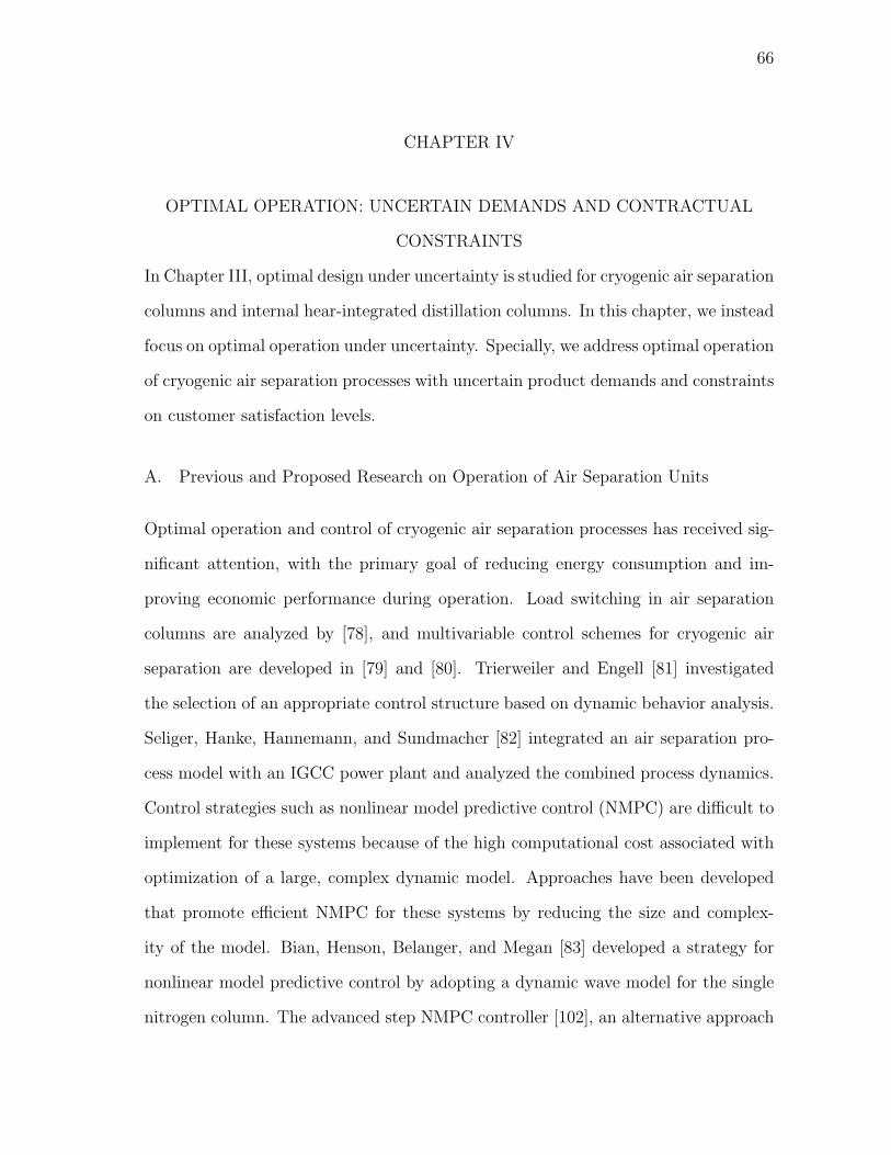
teaching. His insights and perception on novel approaches inspired me tremendously.
It was my great pleasure to work with him.
I also would like to acknowledge the helpful comments and advice I received from
my committee members: Dr. Juergen Hahn, Dr. Mahmoud El-Halwagi, Dr. M. Sam
Mannan from the Chemical Engineering (ChE) Department and Dr. Sergiy Butenko
from the Industrial and Systems Engineering (ISE) Department.
In addition to my PhD study, I am pursuing my Masters degree in Industrial
Engineering. I would like to acknowledge all of the people helping me on transfer-
ring between different departments. They are Dr. Daniel Shantz (ChE), Towanna
Arnold (ChE), Dr. Guy Curry (ISE), Judy Meeks (ISE), Andrea Reinertson (OGS),
and Marisa Ernst(ISS). Without their help, I could not pursue two major degrees
simultaneously.
Bill Morrison, Kiran Sheth, Tyler Soderstrom, Yang Zhang, John Hedengren Carl
Schwanke, Jitendra Kadam, Tonya Donatto, and Weijie Lin deserve special thanks,
as does my boss and my colleagues when I interned at the Core Process Control
Department of ExxonMobil Chemicals in Baytown Texas, USA. In particular, I would
like to thank Bill and Tonya for their kind help and support. I thank Kiran and Tyler
for their technical guidance and advice, and thank Yang, John, Carl, Jitendra and
Weijie for our inspiring discussions. They have helped me to understand the many
challenges that arise in industrial practice.
Page 7
vii
During the summer of 2010, I had the opportunity to work for Bayer AG, in
Baytown Texas, USA as an intern in the Process Dynamics & Optimization Group. I
would like to acknowledge Shoujun Bian, Samrat Mukherjee, David Chen, Xiangmin
Hua, Doug Klenke, Randy Garabedian and Ajay Singh for their kind help during
my internship. All of them provided me important experience on the application of
advanced control solutions in operational plants.
From September 2010 to November 2010, I worked for Modelon AB in Lund,
Sweden as a research intern with Hubertus Tummescheit, Johan Akesson, Katrin
Prolss, and Stephane Velut. This internship experience broadened my perspective on
the advanced modeling and optimization. I would like to thank them for extensive
discussions and strong encouragement on interesting research projects. It was an
amazing experience in self improvement.
I would like to acknowledge all of the past and present members of Dr. Laird’s
group: Ahmed Rabie, George Abbott III, German Oliveros, Jaime Tellez, James
Young, Scott Kolodziej, Kristen Young, Derrick Thomas, Angelica Wong, Brandon
Barrera, Daniel Word, Sean Legg, Jia Kang, and Gabe Hackebeil. I do cherish the
happy time we had together. And thank them for making my office hours so enjoyable.
In addition, I am indebted to my peer colleagues, Chuili Sun, Yunfei Chu, Cheryl
Qu, Zuyi Huang, Mitch Serpas, Loveleena Bansal, Shreya Maiti, Buping Bao, Fuman
Zhao, Nan Shi, Xin Jin, Rongbing Han, Qingqing Wang, Qun Ma, Xin Qu, Peng
Lian, Yuan Lu, Xiaole Yang, Ruifeng Qi, Qingsheng Wang, and Peng He. I thank
them for providing a stimulating and fun environment where I could learn and grow
up.
Finally, and most important, I must thank my parents Benxian Zhu and Jianling
Wang, as well as my wife, Yue Wang, for their unflagging love and support. Without
their support and encouragement, this dissertation would have simply been impossible
Page 8
viii
and I could not have come this far. It is to them I dedicate my dissertation.
Page 9
ix
TABLE OF CONTENTS
CHAPTER Page
I INTRODUCTION . . . . . . . . . . . . . . . . . . . . . . . . . . 1
A. Nonlinear Optimization with Rigorous Large Scale Models 1
B. Chemical Applications of Nonlinear Optimization . . . . . 2
1. Design under Uncertainty . . . . . . . . . . . . . . . . 3
2. Optimal Operations with Steady State Models . . . . 4
3. Real Time Optimization and Control . . . . . . . . . . 6
4. Process Estimation . . . . . . . . . . . . . . . . . . . . 8
C. Challenges of NLP Optimization . . . . . . . . . . . . . . . 9
1. Multiple Units . . . . . . . . . . . . . . . . . . . . . . 10
2. Uncertainty . . . . . . . . . . . . . . . . . . . . . . . . 11
3. Dynamic Systems . . . . . . . . . . . . . . . . . . . . 12
4. Multiperiod Problems . . . . . . . . . . . . . . . . . . 13
5. Spatial Complexity . . . . . . . . . . . . . . . . . . . . 14
D. Dissertation Outline . . . . . . . . . . . . . . . . . . . . . 14
II IPOPT ALGORITHM AND ITS PARALLEL DEVELOPMENT 17
A. SQP Algorithm . . . . . . . . . . . . . . . . . . . . . . . . 18
B. Interior Point Algorithm . . . . . . . . . . . . . . . . . . . 20
1. Basic Framework . . . . . . . . . . . . . . . . . . . . . 21
2. Description of IPOPT Solver . . . . . . . . . . . . . . 22
C. Parallel Computing Applications in Chemical Process
Engineering . . . . . . . . . . . . . . . . . . . . . . . . . . 26
D. Internal Decomposition . . . . . . . . . . . . . . . . . . . . 27
E. Development of Parallel Interior Point Algorithm with
Internal Decomposition . . . . . . . . . . . . . . . . . . . . 28
III DESIGN UNDER UNCERTAINTY . . . . . . . . . . . . . . . . 36
A. Multi-scenario Programming Approaches . . . . . . . . . . 37
B. Case Study 1: Design under Uncertainty for Cryogenic
Air Separation Units . . . . . . . . . . . . . . . . . . . . . 39
1. Current Research about Air Separation Systems . . . 40
2. Uncertainties in Air Separation Process . . . . . . . . 41
3. Process Description . . . . . . . . . . . . . . . . . . . 42
Page 10
x
CHAPTER Page
4. Mathematical Steady State Model of Air Separa-
tion Columns . . . . . . . . . . . . . . . . . . . . . . . 44
5. Mathematical Formulation for Conceptual Design
under Uncertainty . . . . . . . . . . . . . . . . . . . . 48
6. Numerical Results . . . . . . . . . . . . . . . . . . . . 50
7. Conclusions and Future Work . . . . . . . . . . . . . . 54
a. Summary and Conclusions . . . . . . . . . . . . . 54
b. Future Work . . . . . . . . . . . . . . . . . . . . . 55
C. Case Study 2: Design under Uncertainty for Internal
Heat-integrated Distillation Columns . . . . . . . . . . . . 57
1. Process Description . . . . . . . . . . . . . . . . . . . 57
2. Mathematical Model of the Process . . . . . . . . . . 58
a. Conceptual Design Formulation . . . . . . . . . . 60
3. Controllability Constraints . . . . . . . . . . . . . . . 61
4. Optimal Results . . . . . . . . . . . . . . . . . . . . . 62
IV OPTIMAL OPERATION: UNCERTAIN DEMANDS AND
CONTRACTUAL CONSTRAINTS . . . . . . . . . . . . . . . . 66
A. Previous and Proposed Research on Operation of Air
Separation Units . . . . . . . . . . . . . . . . . . . . . . . 66
B. Optimization Formulation and Case Studies . . . . . . . . 69
1. Formulation of Uncertain Demands and Customer
Satisfactions . . . . . . . . . . . . . . . . . . . . . . . 69
2. Case Study 1: Optimal Single Period Operation
with a Single Fill Rate Constraint . . . . . . . . . . . 75
3. Case Study 2: Optimal Single Period Operation
with Multiple Fill Rate Constraints . . . . . . . . . . 79
4. Case Study 3: Optimal Multiperiod Operation with
Multiple Fill Rate Constraints . . . . . . . . . . . . . 82
C. Summary and Conclusions . . . . . . . . . . . . . . . . . . 85
V OPTIMAL OPERATIONS: UNCERTAIN DEMANDS, CON-
TRACTUAL CONSTRAINTS, AND VARIABLE POWER
PRICES . . . . . . . . . . . . . . . . . . . . . . . . . . . . . . . 88
A. Introduction . . . . . . . . . . . . . . . . . . . . . . . . . . 88
B. Multiple Period Operation Formulation . . . . . . . . . . . 90
C. Optimal Operating Strategy under Constant Product
Demands . . . . . . . . . . . . . . . . . . . . . . . . . . . . 96
Page 11
xi
CHAPTER Page
D. Optimal Operating Strategy under Uncertain Product
Demands . . . . . . . . . . . . . . . . . . . . . . . . . . . . 99
E. Conclusions and Future Work . . . . . . . . . . . . . . . . 105
VI DYNAMIC OPTIMIZATION UNDER UNCERTAINTY . . . . 107
A. Introduction . . . . . . . . . . . . . . . . . . . . . . . . . . 107
B. Dynamic Model of the Cryogenic Air Separation Process . 108
1. Mass Balances . . . . . . . . . . . . . . . . . . . . . . 109
2. Energy Balances . . . . . . . . . . . . . . . . . . . . . 110
3. Hydraulic Equation . . . . . . . . . . . . . . . . . . . 110
4. Summation Equation . . . . . . . . . . . . . . . . . . 111
5. Vapor-liquid Equilibrium . . . . . . . . . . . . . . . . 111
6. Pressure Equation . . . . . . . . . . . . . . . . . . . . 111
7. Heat Integration . . . . . . . . . . . . . . . . . . . . . 112
8. Safety Inequality Constraints . . . . . . . . . . . . . . 113
C. Simultaneous Dynamic Optimization Approach . . . . . . 113
D. Optimal Control Results . . . . . . . . . . . . . . . . . . . 115
E. Conclusions . . . . . . . . . . . . . . . . . . . . . . . . . . 116
VII SPATIAL DECOMPOSITION OF CITY-WIDE PIPELINE
NETWORK . . . . . . . . . . . . . . . . . . . . . . . . . . . . . 118
A. Problem Description . . . . . . . . . . . . . . . . . . . . . 118
B. Mathematical Formulation . . . . . . . . . . . . . . . . . . 120
C. Spatial Decomposition . . . . . . . . . . . . . . . . . . . . 121
D. Numerical Results . . . . . . . . . . . . . . . . . . . . . . . 122
VIII CONCLUSIONS . . . . . . . . . . . . . . . . . . . . . . . . . . . 124
A. Summary and Contributions . . . . . . . . . . . . . . . . . 124
1. Summary of All Case Studies . . . . . . . . . . . . . . 125
2. Challenges and Experience . . . . . . . . . . . . . . . 129
3. Parallel Computing . . . . . . . . . . . . . . . . . . . 130
a. Scalability . . . . . . . . . . . . . . . . . . . . . . 131
b. Distributed and Multi-core Architectures . . . . . 131
B. Future Work . . . . . . . . . . . . . . . . . . . . . . . . . . 132
1. NLP Application . . . . . . . . . . . . . . . . . . . . . 133
a. Integration of IPOPT with Other Software . . . . 133
b. Air Separation Units . . . . . . . . . . . . . . . . 133
2. Parallel Computing Development . . . . . . . . . . . . 135
Page 12
xii
CHAPTER Page
REFERENCES . . . . . . . . . . . . . . . . . . . . . . . . . . . . . . . . . . . 138
VITA . . . . . . . . . . . . . . . . . . . . . . . . . . . . . . . . . . . . . . . . 153
Page 13
xiii
LIST OF TABLES
TABLE Page
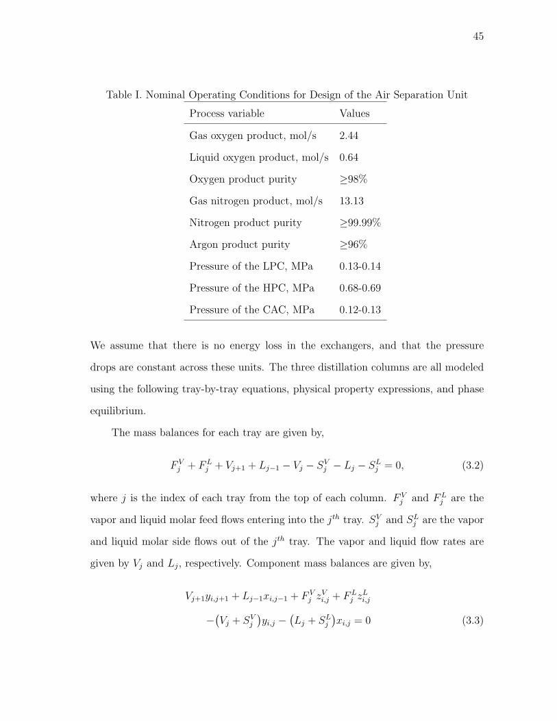
I Nominal Operating Conditions for Design of the Air Separation Unit 45
II Optimal Design for the Nominal and Multi-scenario Formulation
of the Air Separation Unit . . . . . . . . . . . . . . . . . . . . . . . . 53
III Design Results with/without Considering Uncertainties and Con-
trollability (HIDiC) . . . . . . . . . . . . . . . . . . . . . . . . . . . . 63
IV Nominal Operating Conditions for Planning with Customer Sat-
isfaction of the Air Separation Process . . . . . . . . . . . . . . . . . 70
V Standard Deviations of Uncertain Product Demands of ASU planning 83
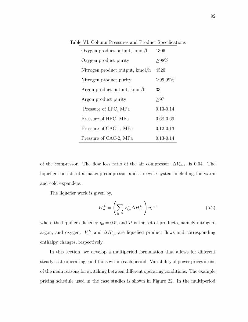
VI Column Pressures and Product Specifications . . . . . . . . . . . . . 92
VII Mean Product Demands and Fill-rate over Four Time Periods . . . . 103
VIII Results for Different Standard Deviations in Argon Demand . . . . . 103
IX Nominal Operation Conditions of Dynamic Optimization in Cryo-
genic ASC Systems . . . . . . . . . . . . . . . . . . . . . . . . . . . . 109
Page 14
xiv
LIST OF FIGURES
FIGURE Page
1 Nonlinear Optimization Applications in Chemical Engineering . . . . 3
2 Redesign IPOPT Structure with Specialized NLP and Linear Al-
gebraic Implementation . . . . . . . . . . . . . . . . . . . . . . . . . 34
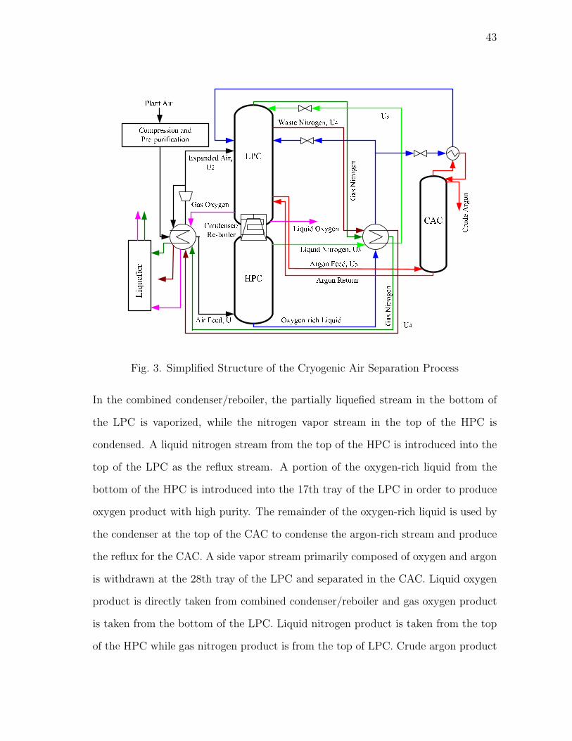
3 Simplified Structure of the Cryogenic Air Separation Process . . . . . 43
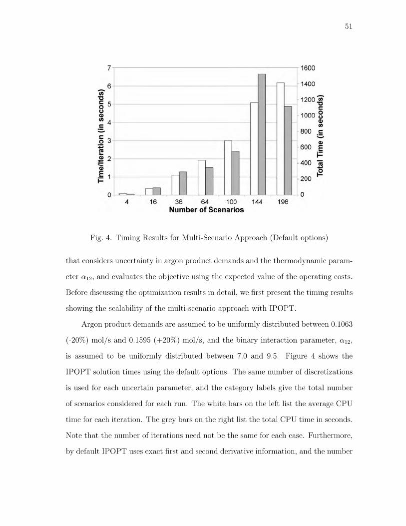
4 Timing Results for Multi-Scenario Approach (Default options) . . . . 51
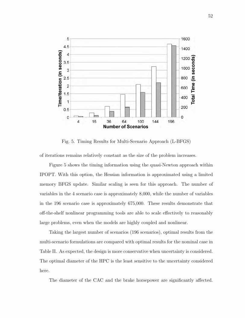
5 Timing Results for Multi-Scenario Approach (L-BFGS) . . . . . . . . 52
6 Dependence between Multi-scenario Design and Increasing Sce-
nario Number . . . . . . . . . . . . . . . . . . . . . . . . . . . . . . . 54
7 Simplified Structure of Internal Heat-integrated Distillation Column . 57
8 Parallel Scalability Results of Schur-IPOPT on a Multi-core System . 64
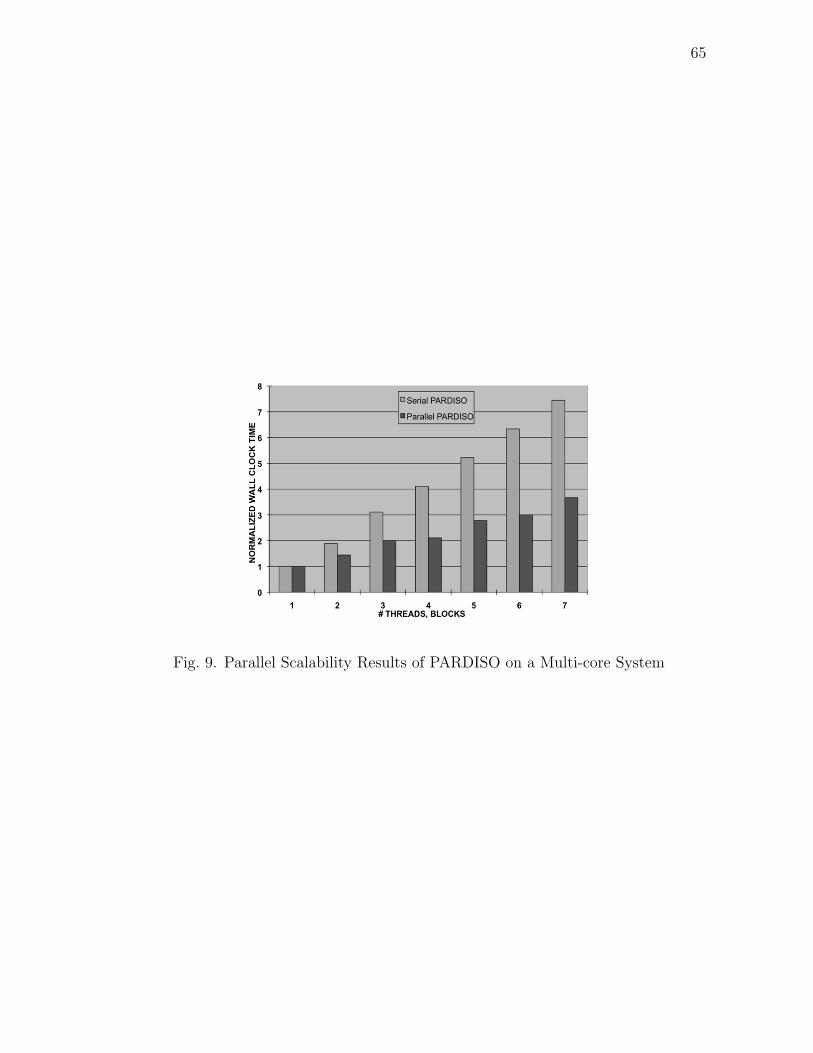
9 Parallel Scalability Results of PARDISO on a Multi-core System . . . 65
10 Optimal Operating Strategies as a Function of N2 Fill Rate (Solid
Line: without Inventory, Dash Line: with Inventory) . . . . . . . . . 76
11 Optimal Operating Strategies as a Function of Ar Fill Rate (Solid
Line: without Inventory, Dash Line: with Inventory) . . . . . . . . . 77
12 Optimal Operating Strategies as a Function of O2 Fill Rate (Solid
Line: without Inventory, Dash Line: with Inventory) . . . . . . . . . 78
13 Feasible Region and Profit Changes as a Function of Nitrogen and
Oxygen Fill Rates without Considering Inventory . . . . . . . . . . . 79
14 Feasible Region and Profit Changes as a Function of Nitrogen and
Argon Fill Rates without Considering Inventory . . . . . . . . . . . . 80
Page 15
xv
FIGURE Page
15 Feasible Region and Profit Changes as a Function of Oxygen and
Argon Fill Rates without Considering Inventory . . . . . . . . . . . . 80
16 Optimal Expected Profit and Inventory under Nitrogen-Oxygen
Fill Rate Constraints with Product Storage . . . . . . . . . . . . . . 81
17 Optimal Expected Profit and Inventory under Nitrogen-Argon Fill
Rate Constraints with Product Storage . . . . . . . . . . . . . . . . . 81
18 Optimal Expected Profit and Inventory under Oxygen-Argon Fill
Rate Constraints with Product Storage . . . . . . . . . . . . . . . . . 81
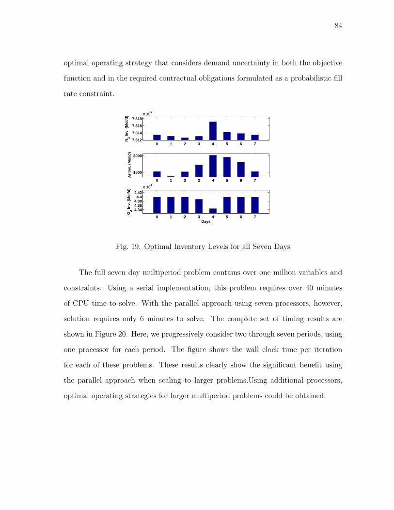
19 Optimal Inventory Levels for all Seven Days . . . . . . . . . . . . . . 84
20 Wall Clock Time per Iteration for Serial and Parallel Approaches . . 85
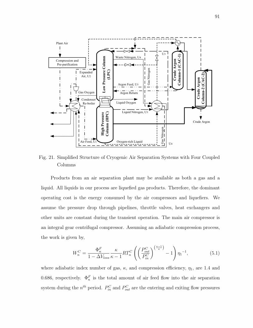
21 Simplified Structure of Cryogenic Air Separation Systems with
Four Coupled Columns . . . . . . . . . . . . . . . . . . . . . . . . . 91
22 Four Periods of Daily Operation Associated with Peak/Off-Peak
Power Pricing . . . . . . . . . . . . . . . . . . . . . . . . . . . . . . . 93
23 Air Feed Flow Load Change under Peak vs. Off-peak Power Pricing . 95
24 Profiles for Total Air Feed Flow Rate (Vfe) and Production Rates
of Each Component (SP). The Solid Lines Represent the Optimal
Values When Operating Conditions Are Forced to Be Constant,
and the Dashed Lines Represent the Multiperiod Solution . . . . . . 98
25 Optimal Results for Inventory Levels (inv) and Manipulated Vari-
ables (U) in the Multiperiod Case . . . . . . . . . . . . . . . . . . . . 98
26 Optimal Trajectories of Oxygen, Argon and Nitrogen Products,
and Manipulated Variables under Nominal (Dashed) and Uncer-
tain (Solid) Pressure Drops of the LPC. . . . . . . . . . . . . . . . . 116
27 Wall Clock Time per Iteration for Serial and Parallel Approaches
of Optimal Control under Uncertainty . . . . . . . . . . . . . . . . . 117
28 Structure of Large Water Network with Seven Sub-parts . . . . . . . 119
Page 16
xvi
FIGURE Page
29 Structure of Splitting Network by One-input-one-output Node:
(a) Original Nodes Without Splitting; (b) Updated Nodes After
Splitting . . . . . . . . . . . . . . . . . . . . . . . . . . . . . . . . . . 122
30 Wall Clock Time per Iteration for Serial and Parallel Approaches . . 123
Page 17
1
CHAPTER I
INTRODUCTION
The objective of this dissertation is to develop powerful nonlinear programming al-
gorithms and to solve complicated optimization problems arising from large-scale
chemical engineering processes. In this chapter, we describe the overall motivation
and challenges on when determining optimal decisions of chemical processes with
rigorous first-principle models and developing nonlinear programming approach. In
addition, we introduce background information and terminology used throughout this
dissertation.
A. Nonlinear Optimization with Rigorous Large Scale Models
With growing appreciation of large-scale rigorous models which are based on first
principles, nonlinear optimization has also become an effective tool to obtain profit
gain through process design and operations in chemical and petroleum industries.
Large scale rigorous nonlinear models are preferred and often required due to
three main considerations. The first reason is non-linearity of the chemical process
itself. Highly nonlinear behaviors are well known characteristics in most chemical
processes. In models of reaction units or separation units, fundamental principles
including complex phase and reaction equilibrium, hydraulics, as well as mass and
energy balances, are often governed by highly nonlinear equations. In many cases,
linear models can not capture process behavior completely and accurately, resulting
in large mismatch between the model and plant. Secondly, increasing market com-
petitions drive modern petroleum, chemical and gas companies to pursue the higher
The journal model is IEEE Transactions on Automatic Control.
Page 18
2
profitability of their plants and meet better customer satisfaction. Companies not
only focus on stable production and operation as before, but also desire fast, timely
response to market changes. Market changes include product demands and prices,
material prices and customer satisfaction, and environmental regulations. Therefore,
it is necessary to include more and more market information into large scale rigorous
models. The third reason concerns the range of model validity. Although data-drive
models are still used in many applications, the most important advantage of rigorous
first principle models is their large range of validity. For example, the models iden-
tified by step or impulse responses can be adopted in dynamic control applications.
However, such identified models are not suitable and reliable for optimal design and
planning problems.
Optimization (the inverse problem) is more challenging than simulation (the for-
ward problem), and state of the act simulation models are usually more complex than
those used for optimization. However, the requirement of optimal decision making
for complicated chemical process design and operations seriously pushes the demands
to adopt rigorous models in optimization problems, and our desire is to close this
gap. With the development of nonlinear optimization algorithms and continuously
increasing computing power, it is more and more possible for us to obtain reliable
optimal solutions from rigorous mathematical formulations.
B. Chemical Applications of Nonlinear Optimization
There are several important applications of nonlinear optimization in the chemical
engineering field. The interaction and relationship among some of these applications
is given in Figure 1. Several case studies from these application areas are selected
in this dissertation in order to show how to efficiently solve large scale nonlinear
Page 19
3
optimization problems with rigorous models.
Fig. 1. Nonlinear Optimization Applications in Chemical Engineering
1. Design under Uncertainty
At the design stage, engineers not only focus on the unit structure and cost, must
consider how increasing flexibility of operation can affect future operations (especially
given significant uncertainty).Before a process design can be started, the design prob-
lem must be formulated, which asks for a product specification. After the product
design, process design addresses how to transform raw materials into desired chemical
products using the most suitable process structures and operating parameters. Tradi-
tional process design assumes the process operating capacity stays in a narrow range.
However, in modern market-oriented design and operating problems, increased flexi-
bility of the process is required to make fast operating changes. Increasing operating
flexibility asks process designers to take market uncertainty into account [1]. Without
rigorous consideration of uncertainty at the design stage, process flexibility is limited
Page 20
4
and the plant may not effectively handle exogenous disturbances (e.g. changes in
products demands and prices as well as raw material prices).
In order to handle potential uncertainties at design stage, the traditional ap-
proach is to design the process according to nominal values of the uncertain parame-
ters and then apply empirical overdesign factors. However, this method may not be
reliable and can lead to infeasible designs. It is certainly not guaranteed to be optimal.
Instead of the traditional overdesign method, nonlinear optimization can be adopted
to rigorously treat uncertainties. The main goal of the optimal design problem is to
determine optimal values of the desire variables, minimize or maximize the expected
value of economic function over the uncertainty space, maintain feasibility over the
the uncertainty space, and ensure customer satisfaction. This can be treated with
both probabilistic constraints and multiscenario formulations. In the later chapter of
this dissertation, we discuss how to deal with different kinds of uncertain factors and
obtain optimal design solutions for large scale chemical processes.
2. Optimal Operations with Steady State Models
After the design stage, the structures of processes and some process parameters are
fixed during the operation stage. This stage can be separated into several parts. The
top part is the planning and scheduling layer, which makes long-term decisions like
which products to produce, when and how to produce, then how to control inventory
level, in order to earn profit and maintain customer satisfaction. Forecasts of market
information like product demands and prices are used to obtain best estimation of the
optimal decisions for future operations (years/months/weeks). Because this layer has
a strong relationship with market, it is very important for managers and engineers
to make planning and scheduling decisions with consideration of various customer
satisfactions and uncertain market factors. These high-level decisions are often made
Page 21
5
using linear models. However, such linear models can not capture detailed process
interactions. Poor planning/scheduling decisions may challenge lower-level practical
operation due to both inaccurate market forecast and inaccuracies from linear black-
box process models.
Instead of linear black-box process models, rigorous nonlinear models can be
adopted to provide more accurate information of process behaviors. All the opera-
tional planning and real-time optimization using steady state models are typically im-
posed. However, prices of raw materials, energy, and products can change frequently.
Correspondingly, product demands may also change. Due to external markets, pro-
cess inputs and requirements are subject to both variability and uncertainty. It is
necessary to consider these factors and often multiperiod problem formulations are
used.
Furthermore, the conflicts between customer satisfaction and profitability should
also be taken into account. if we only focus on high short-term profit and ignore cus-
tomer satisfaction, nonlinear optimization problems do not need to include constraints
from customer satisfactions and the plant profit can be maximized. As time goes by,
we may lose customers or violate contracts because their demands can not be ade-
quately satisfied. In order to handle uncertain product demands from customers and
guarantee high customer satisfaction, sufficient inventory levels have to be kept. How-
ever, it is undesirable from a cost perspective to keep high inventory levels. Therefore,
multiperiod optimization formulations can be solved to maximize profits while main-
taining contractual obligations. These formulations provide managers with the tools
necessary to evaluate the trade-off between short-term profitability and customer
satisfaction in this level.
In this dissertation, we adopt nonlinear programming formulations with rigorous
models to handle energy cost variability and uncertainty in product demands with
Page 22
6
multiperiod inventory planning.
3. Real Time Optimization and Control
Real-time optimization (RTO) is the next layer which follows the planning and
scheduling layer. The objective of the RTO is to maximize economic performance
of the plant by seeking the detailed optimal operating conditions, based on current
process information and decisions from higher level (planning and scheduling level).
Therefore, this layer needs to optimize operating conditions in real-time according to
the market changes of product price and demands. RTO can be separated into two
different kinds of approaches: steady state and dynamic. Traditional steady-state
RTO has already been applied widely in the process, and closed-loop steady-state
RTO bring increased profits compared with traditional process control alone [2].
However, traditional steady-state RTO has some drawbacks. the first is low fre-
quency. It is normal to run twice or three times per day. second, it does not rigorously
consider the cost of transiting from one operating condition to another. Some plants
need to respond market changes very quickly, like grade change in polymerization
and petroleum process, as well as load changes in cryogenic air separation processes.
In these processes, market competition requires the capability to accomodate fast
and cost effective transitions so that companies can produce and sell on demand at
favorable prices. To provide this capability, dynamic RTO is being developed and
implemented in industrial processes. The largest difference between steady state and
dynamic RTOs is that traditional RTO only provides optimal operating conditions at
one steady state time point, while dynamic RTO provides a trajectory of operating
condition changes. As an analogy, traditional GPS only tells us our next location,
while advanced GPS can tell us a complete pathway by following the dynamic tra-
jectory it provides. Dynamic RTO does not require steady-state conditions to start
Page 23
7
an optimization, and it enables shorter transition times. Shorter transition times
generally result in reduction of off-specification material and therefore increased prof-
itability of a plant.
Dynamic RTO is usually formulated using large-scale nonlinear dynamic process
model. The resulting optimization problem must be solved quickly and however,
computational complexity and efficiency is the largest challenge for the dynamic RTO.
With the set-points or trajectories provided by the RTO layer, the process con-
trol layer drives the plant along these optimal operating conditions while keeping the
plant safe and stable. Currently, traditional PID controllers are stilled widely applied
in practice, because of their cheap price and acceptable performance. When higher
control performance is required by fast market changes and smaller operating mar-
gins, Model Predictive Control (MPC) has been adopted by a lot of plants because it
provides faster process responses and more suitable control actions than traditional
PID controllers. The main advantage of MPC, compared with the traditional PID
controllers, is that it can handle multi-variable interactions through the model. Cur-
rently, the MPC can be separated into two categories: linear and nonlinear. Early
MPC strategies like Dynamic Matrix Control (DMC)[3] uses a linear process model
and it can provide optimal control actions by on-line minimization of the control
objective function. A good review of industrial MPC applications can be found in
[4]. However, the control performance of the linear MPC is limited when there is
a significant mismatch between the linear models and true process behavior, either
because of a highly nonlinear process, or a wide operating range. Therefore, non-
linear MPC using rigorous models has received increasing industrial and academia
attention. Rigorous first-principle models are able to significantly reduce the mis-
match between process and model. However, as with Dynamic RTO, nonlinear MPC
also has significant computational challenges to provide fast solutions and meet on-
Page 24
8
line requirements. With development of advanced numerical algorithm and improved
hardware, it is a trend to adopt nonlinear MPC and improve control performance.
Both the dynamic RTO and the nonlinear MPC are large scale dynamic opti-
mization problems which have a lot of differential and algebraic equations (DAE) as
constraints. There are several methods adopted to solve the DAE optimization prob-
lems. In our process industry, main approaches are all based on NLP solvers. These
approaches can be separated into three categories, sequential, multiple-shooting, and
simultaneous strategies. In the sequential methods, also known as control vector
parameterization, only control variables are discretized, and these are typically rep-
resented as piece-wise polynomials. A DAE solver is used within an inner loop for
integration of DAE system while a NLP solver is adopted at outer loop for solving
the optimization. In simultaneous approaches, both the state and control profiles are
discretized in time, typically using collocation of finite elements. There is no defini-
tive conclusion about which approach (sequential and simultaneous) is more suitable
for large scale dynamic optimization problems since researchers are developing better
algorithms to exploit structure and provide computationally cheap approximations
for both strategies. In general, simultaneous approaches may be more suitable to
deal with DAE optimization problems which include a lot of degrees of freedom. Si-
multaneous approaches are adopted by this dissertation to deal with rigorous DAE
optimization problems, such as Dynamic RTO or nonlinear MPC. In order to obtain
more reliable solutions, uncertain disturbances transients are considered.
4. Process Estimation
Both the RTO and the nonliner MPC mentioned above depend on rigorous mathemat-
ical models of the industrial process. These models are often developed by repetitive
model discrimination and experimental design. After the original model structures
Page 25
9
are fixed, model parameters are tuned based on on-line data extracted and measured
from the full-scale process. Therefore, whatever on-line or off-line, parameter estima-
tion plays a critical role for further development of reliable models. As an analogy,
consider the GPS (the RTO) and the driver (the controller) which need to know the
information about weather and traffic conditions provided from the estimation part,
in order to make good decisions. Sometimes, the RTO and MPC may provide bad
operating decisions due to inaccurate state and parameter estimation.
Nonlinear programming is an effective framework for reliable parameter esti-
mation, by minimizing the objective function associated with differences between
estimated and measured variables under rigorous formulations of the process model
as constraints. In many cases, the model is very complex and the number of data is
so large that the estimation problems are very challenging and require powerful non-
linear programming approaches. Here, in the later chapter of this dissertation, we are
interested in exploiting the advantages of modern computing architecture and com-
putational strategies to solve estimation problems incorporating large-scale process
models.
C. Challenges of NLP Optimization
In the previous section, several important problem classes for chemical process en-
gineering were discussed in the areas of optimal design, operation, and parameter
estimation. The use of rigorous nonlinear models is desired to increase model fidelity
and improve solutions, however, this also increases the size and complexity of the NLP
formulation. This issue is further intractable with consideration of model variability
and uncertainty.
The desire to reduce mismatch between models and processes pushes people to
Page 26
10
adopt rigorous first-principle models. Mass and energy balances are required in such
rigorous models. Rigorous thermodynamic approaches like activity coefficients and
equations of state (EOS) are more frequently adopted in process models for design
and operations, compared to previously used relative volatility methods. These com-
plex mathematical descriptions lead to high order implicit equations which are very
difficult to solve. As well, the number of variables increases significantly when more
complex equations are adopted. In general, rigorous descriptions increase the number
of variables by more than a factor of two over simple models [5]. It is a rough estima-
tion that approximately 60% of computational load is resulted from solving rigorous
thermodynamic and kinetic equations in simulation and optimization [5]. When all
equality and inequality constraints consists of the rigorous model equations (balance
equations, thermodynamic and kinetic relationships etc.), the size of problems is very
huge, however, the Jacobian of the constraints is typically very sparse.
Besides complexity from the models themselves, rigorous nonlinear optimization
problems are very challenging due to other important factors. Here, we want to
briefly discuss these factors which increase difficulty when solving rigorous nonlinear
optimization problems. Problem sizes continue to grow, and parallel nonlinear op-
timization algorithms are developed in order to handle these factors well and solve
practical nonlinear optimization problems with high computational efficiency.
1. Multiple Units
Because of interactions between highly coupled process units or enterprise activities,
both industry and academia are interested in including more of product, process, and
enterprise life cycle under the umbrella of a single integrated optimization problem.
Enterprise or plant-wide optimization has received an increasing attention during re-
cent decades [6]. The operating condition changes of one unit not only have an impact
Page 27
11
on its own energy efficiency and economic performances, but can also significantly af-
fect the performance of its upstream and downstream units. For example, in cryogenic
air separation systems, there are three high coupled columns (High-pressure column,
HPC, low-pressure column, LPC and crude argon column, CAC). When temperature
of the HPC decreases, due to heat integration between the HPC and the LPC, the
upward stream rates in LPC also decrease correspondingly. Furthermore, increases in
the the nitrogen concentrations in side withdrawal flows to the CAC can lead to un-
stable operations when producing argon products. Therefore, it is often necessary to
consider many units within a simple optimization framework. The optimal solutions
from plant-wide optimization can provide more reliable decisions than those obtained
from single-unit optimization, and may also avoid dangerous operating situations such
as snowball effects from recycle operations.
Increasingly, local optimizations over a single unit are replaced by entire plant-
wide formulations. If each unit model is developed according to its own first principles,
the number of process variables in the rigorous plant-wide optimization problems are
close to the sum of all single unit model variables. For instance, the number of vari-
ables within cryogenic air separation systems may be several times of a conventional
distillation column. Large problem size and strong interactions among different units
result in increased difficulty and computational complexity.
2. Uncertainty
Uncertainty always exists in process design and operation.Uncertain process distur-
bances and market variability affect process performance and profit. In order to make
reliable decisions, uncertainty should be rigorously considered within the optimization
framework.
There are two main approaches to deal with uncertainty. One is based on a
Page 28
12
probabilistic or chance constraints and the other is based on the use of multiscenario
formulations. Both these strategies are used to address uncertain in this dissertation,
however, the multisecnerio approach causes significant increases in the problem size.
Typically, the continuous uncertainty space is discretized into different individual sce-
nario, and the objective function is an expected value over the scenarios. All of these
scenarios are included as constraints to ensure feasibility of each scenario. Individual
scenarios are coupled by stage-1 variables. When we simultaneously consider mul-
tiple uncertain parameters within the same optimization framework, the sizes and
complexities of nonlinear optimization problems increase exponentially. For example,
there are 3 uncertain parameters we need to focus on in our process. Each parameter
has its own uncertain range and we separate each uncertain range by selecting 10
sampling points. So, there are 103 scenarios in total. Therefore, considering more
uncertainties can increase sizes of nonlinear optimization problems significantly. Fur-
thermore, more scenarios can provide more reliable solution. Of course, increasing
the number of scenarios results in larger problem size and heavier computational
requirement.
Large problem size creates the need for advanced approaches. In this disserta-
tion, we exploit the structure these problems and develop an internal decomposition
approach that allows for efficient parallel solution.
3. Dynamic Systems
Several important problem classes in chemical engineering requires optimization of
systems governed by differential-algebraic equations. For design problems, the first-
principle models typically consist of all algebraic equations. However, for dynamic
operations, the rigorous models are fundamentally described by large sets of Differ-
ential and Algebraic Equations (DAEs). Sometimes, partial DAEs may be required
Page 29
13
to describe both spatial and time relationships of process variables.
When we solve dynamic optimization problems using simultaneous strategies,
the differential equations are discretized th and included as constraints to convert
dynamic optimization into a large scale nonlinear optimization problem. The number
of elements and the number of collocation points within each element determine the
size of the resulting NLP. Implicit Runge-Kutta and Radau collocation methods are
often used to keep high order accuracy and excellent stability properties. In this
dissertation, we do not decompose these differential problems in the time domain
(although this can be done and is the subject of current research). Instead, we address
dynamic optimization problems with uncertainty and decompose the multiscenario
structure. These problems are particularly challenging because of the large size of each
individual scenarios. In this dissertation, we are interested in developing powerful
computational strategies and solving rigorous dynamic optimization problems of a
multi-unit chemical plant under uncertainties.
4. Multiperiod Problems
A class of problems that can easily be decomposed is multiperiod problems. When
we are interested in seeking optimal operating solutions for longer term planning and
scheduling, a multiperiod programming approach is often adopted with operating
variables within each period and intermediate variables between the periods, such as
inventory levels. These may be additional benefit in allowing the start and end of
each operating period to change. And these can be considered as variables in the
optimization problem. The interaction between additional periods increases the size
and complexity of the resulting nonlinear optimization problem. A computational
strategy is developed and implemented to efficiently solve a multiple period (weekly)
operating problems under uncertain product demands.
Page 30
14
5. Spatial Complexity
In regions highly concentrated with chemical and petroleum industries, raw mate-
rials and products are often supplied via extensive pipeline networks. Many liquid
products, such as gasoline, liquid oxygen and nitrogen, and water, are all delivered
from the plant to different customers through pipeline networks. As an example, a
middle size oxygen pipeline network is over 50 miles long and has approximately 15
customers and 2 cryogenic air separation plants. Both gasoline and water have more
customers, and a city-wide water network can be quite huge, including hundreds of
thousands of nodes.
Optimization of large scale water network is just one example of a problem with
spatial complexity. This structure can also be decomposed by parallel approach. In
this dissertation, we consider the large-scale inverse problem of demand estimation in
a city-wide water distribution system. First-principle hydraulic models of all pipes,
pumps and other devices need to be included. Spatial complexity imposed by a huge
number of nodes and pipes challenges off-the-shelf nonlinear optimization algorithms.
In Chapter VII of this dissertation, we are interested in efficiently solving a large
scale parameter estimation problem with rigorous process model of a city-wide water
pipeline network. Parallel solution is enabled by decomposing the network spatially.
D. Dissertation Outline
While large-scale nonlinear programming (NLP) has seen widespread use within the
process industries, the desire to solve larger and more complex problems drives contin-
ued improvements in NLP solvers. Because of physical hardware limitations, manufac-
turers have shifted their focus towards multi-core and other modern parallel comput-
ing architectures, and we must focus efforts on the development of parallel computing
Page 31
15
solutions for large-scale nonlinear programming. In this dissertation, we develop a
parallel nonlinear interior point algorithm for problem with block-angular structure.
With the help of this parallel nonlinear optimization algorithm, we focus on
addressing several classes of nonlinear optimization problems including process de-
sign and operation under uncertainties, and parameter estimation. We argue that
these advanced parallel algorithm can tackle larger problems and allow for solution
of previously intractable problems using rigorous nonlinear models. The mentioned
challenges, such as uncertainties, dynamics, and spatial complexity, are addressed in
the following sections of this dissertation.
Chapter II describes the development of nonlinear programming approaches in
chemical process engineering. All problems in this dissertation are solved by the
existing nonlinear solver, IPOPT, or by our parallel interior point approach based
on IPOPT. A brief introduction of the line-search based interior point approach is
introduced and the advantages and disadvantages of this method are discussed. In
the later sections of Chapter II, we describe several applications of parallel computing
including simulation and optimization in the chemical process engineering area. Our
internal decomposition approach based on a schur-complement decomposition of the
KKT system is presented.
The main body of this dissertation discusses the application of these approaches
to the problem classes discussed earlier. Chapter III focuses on optimal design under
uncertainty for large scale cryogenic air separation units (ASU) and internal heat-
integrated distillation columns.
Chapter IV addresses the optimal operating problems under uncertain product
demands and different customer satisfaction levels in cryogenic air separation units.
Chapter V introduces switching time as optimization variables and focuses on ob-
taining optimal daily operating strategies under various power pricing and uncertain
Page 32
16
product demands for large scale cryogenic air separation units. Chapters IV and V
focus on optimal multiperiod operation under uncertainty where steady-state models
are used with each period. Chapter VI solves a dynamic optimization problem under
uncertainty. Using a large-scale differential equation models of an ASU, this chapter
focuses on improving dynamic performance during a load change while considering
process uncertainty. Chapter VII demonstrates a spatial decomposition by solving
a large-scale inverse problem to estimate unknown water demands in a city-wide
network. Several of these problems are solved by our parallel nonlinear algorithm,
in order to demonstrate scalability and the computational benefit of using parallel
computing.
The dissertation closes in Chapter VIII, where general concluding remarks and
recommendations for future work are presented.
Page 33
17
CHAPTER II
IPOPT ALGORITHM AND ITS PARALLEL DEVELOPMENT
Nonlinear programming (NLP) has proven to be an effective framework for obtaining
profit gains through optimal process design and operations in chemical engineering.
However, the scale of the NLP problems we wish to solve continues to grow. More
and more is being included within a single integrated optimization formulation. Mul-
tiple units and products are included in plant-wide and enterprise-wide optimization
problems. In order to reduce plant/model mismatch, the development of increas-
ing rigorous models based on first-principles increases both the size and complexity
of problem formulations. Large-scale NLP problems result when simultaneous dis-
cretization approaches are used to reformulate optimization problems with model
behaviour governed by differential and partial differential equations. Furthermore, to
improve the robustness of optimization solutions, uncertainties in both design and op-
erations may need to be considered. Multi-scenario problem formulations provide an
approach for treating uncertainty, however, these formulations grow with the number
of scenarios. Due to the above considerations, as NLP problems grow increasingly
large and more complicated, they continue to push the development of nonlinear
programming algorithms.
In this chapter, at first, the background of nonlinear programming algorithms
is introduced, focusing on the Successive Quadratic Programming (SQP) approach.
Then, the interior-point approach is introduced and discussed as an alternative to
overcome the large shortcoming of SQP methods. Following this background, we
present our implementation of a parallel interior point approach for the solution of
large-scale block-angular nonlinear programming problems based on a schur-complement
decomposition of the KKT system.
Page 34
18
A. SQP Algorithm
The development of nonlinear programming approaches has been very important for
effective solution of chemical process problems arising from both design and oper-
ations. One of the most important NLP algorithms is Successive Quadratic Pro-
gramming (SQP), which deals with NLP problems by successively solving a series of
quadratic programming (QP) sub-problems in order to obtain a search direction and a
step size for next iteration. the constraints of each QP sub-problem are linearizations
of the constraints in the original problem, and the objective function of sub-problem
is a quadratic approximation of the Lagrangian function. An SQP method was first
introduced by Wilson [7] in 1963 for the special case of convex optimization. The ap-
proach was popularized mainly Biggs [8], Han [9], and Powell [10] for general nonlinear
constraints.
At first, we consider a general nonlinear optimization problems only with equality
constraints for easy explanation of fundamental principles of the SQP algorithm.
minx
f (x)
s.t. c (x) = 0 (2.1)
Here x ∈ Rn, c ∈ Rm and the functions f(x) and ci(x), are assumed to have continuous
second derivatives.
The relevant Lagrangian function for the problem in Equ. (2.1) is
L(x, λ) = f(x) + λT c(x) (2.2)
and the first order optimality conditions are given by,
∇xL = ∇f(x) +m∑i=1
λi∇ci(x) = 0 (2.3)
Page 35
19
c(x) = 0 (2.4)
Our desire is to find a critical point x for the nonlinear optimization problem with
optimal multipliers λ. Given an initial estimate (x0, λ0) of Equ. 2.3 and 2.4, we can
generate a sequence (xk, λk) by,xk+1
λk+1
=
xk
λk
+
dxk
dλk
(2.5)
where the search steps [dxk, dλk ] are obtained by applying Newton’s method to the first
order optimality conditions.
∇2xL(xk, λk) ∇cTk
∇ck 0
dxk
dλk
= −
∇xL(xk, λk)
ck
(2.6)
The final optimal values (x, λ) can be converged by solving Equ. (2.6) repeatedly
with form of line-search to ensure global convergence. In SQP methods, an equivalent
formualtion to Equ. (2.6) can be given by the following QP sub-problem.
mind
∇(xk)Td+
1
2dT∇2
xL(xk, λk)d
s.t. c (xk) +∇c (xk)T d = 0 (2.7)
As for NLP problems with inequality constraints g(x) ≥ 0, we can derive the resulting
QP with a linear approximation of the inequality constraints
minx
∇(xk)Td+
1
2dT∇2
xL(xk, λk)d
s.t. c (xk) +∇c (xk)T d = 0
g (xk) +∇g (xk)T d ≥ 0 (2.8)
Page 36
20
Historically, most SQP algorithms use a positive-definite quasi-Newton approxi-
mation, B, (e.g. BFGS) to replace ∇2xL, removing the need to calculate the Hessian
degrees of freedom. However, enabled by automatic differentiation packages, modern
algorithms are making use of full second order information.
When the total number of variables is often larger than the number of variables,
reduced space SQP algorithms, termed rSQP, have been developed in order to improve
the computational efficiency. There are several available nonlinear software packages
based on the SQP methods such as SNOPT [11], filterSQP [12], NLPQL [13], NPSOL
[14], and DONLP [15].
However, the main shortcoming of SQP and its variants is that these algorithms
require the explicit identification of variable bounds that are active at the solution of
the QP. Barrier methods, based on earlier work by Fiacco and Mccormick [16], avoid
this problem by shifting the bound constraints to the objective function in the form
of a logarithmic barrier term.
B. Interior Point Algorithm
Interior-point methods, [17, 18, 19, 20, 21, 22], remove the combinatorial approach of
identifying the active-set by moving the variable into the objective in the form of a
barrier term. This barrier term penalizes the objective bounds as variable approach
their bond. Sequences of barrier sub-problems are solved to converge the original
problem. Interior point methods have emerged as highly efficient techniques and
are currently considered among the most powerful algorithms for large-scale NLP
problems [23].
Page 37
21
1. Basic Framework
Here, we briefly introduce the fundamental principles of interior point methods. Con-
sider the NLP problem:
minx
f (x)
s.t. c (x) = 0
g (x) ≥ 0 (2.9)
where f : Rn → R, c : Rn → Rq, and g : Rn → Rm are assumed to have continuous
second derivatives. With slack variables, s, Equ. (2.9) can be modified to give,
minx
f (x)
s.t. c (x) = 0
g (x)− s = 0
s ≥ 0 (2.10)
The problem form, shifting the bounds to the objective function in the form of a log
barrier term, gives the barrier sub-problems,
minx,s
f (x)− µm∑i=1
log si
s.t. c (x) = 0
g (x)− s = 0 (2.11)
where µ > 0 is called the barrier parameter. When µ approaches zero, the barrier
problem closely approximates the original problem. This sub-problem is solved for a
fixed value of the barrier parameter. then the barrier parameter is decreased as the
problem is solved again.
Page 38
22
2. Description of IPOPT Solver
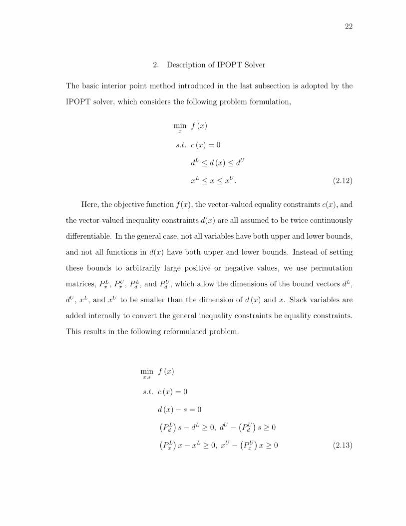
The basic interior point method introduced in the last subsection is adopted by the
IPOPT solver, which considers the following problem formulation,
minx
f (x)
s.t. c (x) = 0
dL ≤ d (x) ≤ dU
xL ≤ x ≤ xU . (2.12)
Here, the objective function f(x), the vector-valued equality constraints c(x), and
the vector-valued inequality constraints d(x) are all assumed to be twice continuously
differentiable. In the general case, not all variables have both upper and lower bounds,
and not all functions in d(x) have both upper and lower bounds. Instead of setting
these bounds to arbitrarily large positive or negative values, we use permutation
matrices, PLx , P
Ux , PL
d , and PUd , which allow the dimensions of the bound vectors dL,
dU , xL, and xU to be smaller than the dimension of d (x) and x. Slack variables are
added internally to convert the general inequality constraints be equality constraints.
This results in the following reformulated problem.
minx,s
f (x)
s.t. c (x) = 0
d (x)− s = 0(PLd
)s− dL ≥ 0, dU −
(PUd
)s ≥ 0(
PLx
)x− xL ≥ 0, xU −
(PUx
)x ≥ 0 (2.13)
Page 39
23
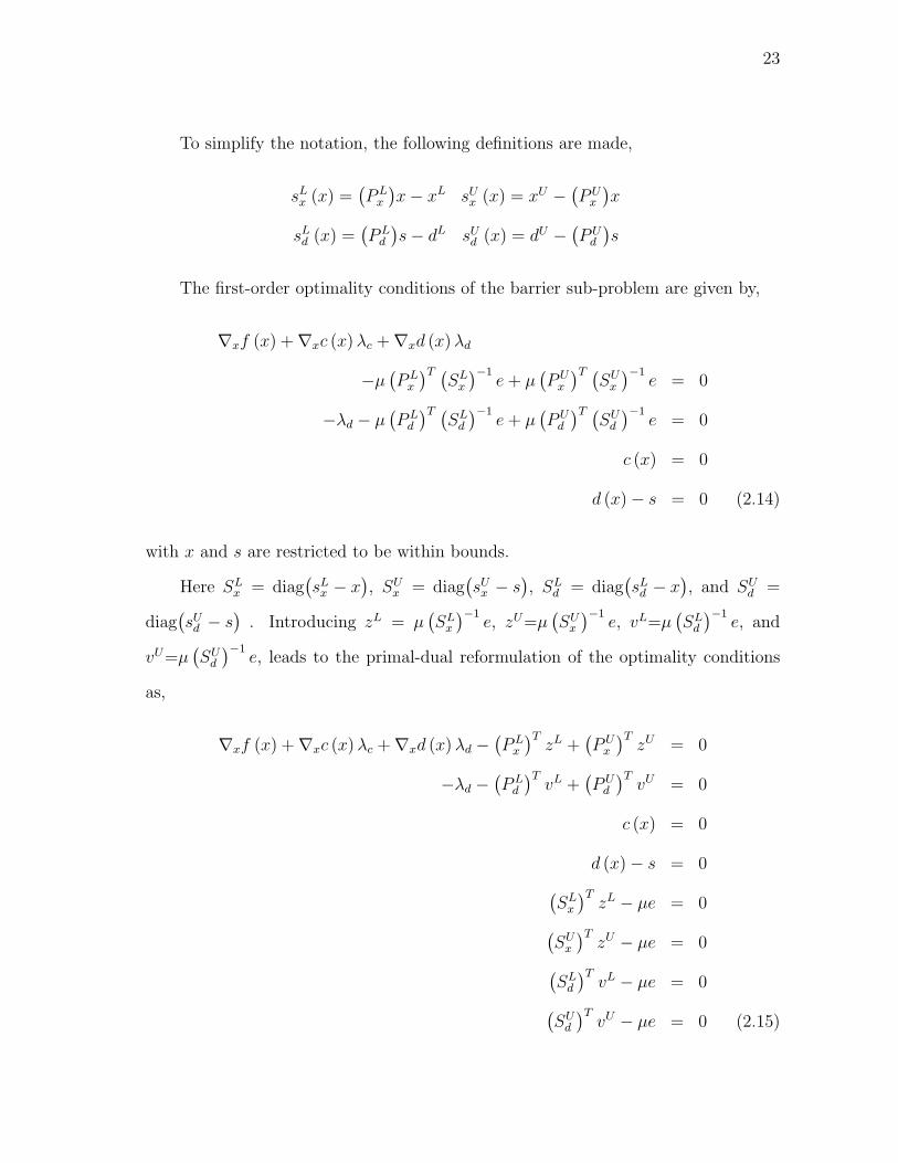
To simplify the notation, the following definitions are made,
sLx (x) =(PLx
)x− xL sUx (x) = xU −
(PUx
)x
sLd (x) =(PLd
)s− dL sUd (x) = dU −
(PUd
)s
The first-order optimality conditions of the barrier sub-problem are given by,
∇xf (x) +∇xc (x)λc +∇xd (x)λd
−µ(PLx
)T (SLx
)−1e+ µ
(PUx
)T (SUx
)−1e = 0
−λd − µ(PLd
)T (SLd
)−1e+ µ
(PUd
)T (SUd
)−1e = 0
c (x) = 0
d (x)− s = 0 (2.14)
with x and s are restricted to be within bounds.
Here SLx = diag
(sLx − x
), SU
x = diag(sUx − s
), SL
d = diag(sLd − x
), and SU
d =
diag(sUd − s
). Introducing zL = µ
(SLx
)−1e, zU=µ
(SUx
)−1e, vL=µ
(SLd
)−1e, and
vU=µ(SUd
)−1e, leads to the primal-dual reformulation of the optimality conditions
as,
∇xf (x) +∇xc (x)λc +∇xd (x)λd −(PLx
)TzL +
(PUx
)TzU = 0
−λd −(PLd
)TvL +
(PUd
)TvU = 0
c (x) = 0
d (x)− s = 0(SLx
)TzL − µe = 0(
SUx
)TzU − µe = 0(
SLd
)TvL − µe = 0(
SUd
)TvU − µe = 0 (2.15)
Page 40
24
with x and s within bounds, and zL, zU , vL, vU ≥ 0.
The Newton step for this system of equations at iteration k is given by,
Hk 0 ∇xc(xk
)∇xd
(xk
)−
(PLx
)T −(PUx
)T0 0
0 0 0 −I 0 0 −(PLd
)T (PUd
)T∇xc
(xk
)T0 0 0 0 0 0 0
∇xd(xk
)T −I 0 0 0 0 0 0(zL
)kPLx 0 0 0
(SLx
)k0 0 0
−(zU
)kPUx 0 0 0 0
(SUx
)k0 0
0(vL
)kPLd 0 0 0 0
(SLx
)k0
0 −(vU
)kPUd 0 0 0 0 0
(SUd
)k
∆x
∆s
∆λc
∆λd
∆zL
∆zU
∆vL
∆vU
=
rx
rs
rc
rd
rLz
rUz
rLv
rUv
(2.16)
where Hk = ∇2xf(xk)+∇2
xc(xk)λkc +∇2
xd(xk)λkd and the right hand side vector is
defined by,
rx = −[∇xf
(xk)+∇xc
(xk)λkc +∇xd (x)λ
kd −
(PLx
)T (zL)k
+(PUx
)T (zU)k]
rs = λkd +
(PLd
)T (vL)k − (PU
d
)T (vU)k
rc = −c(xk)
rd = −d(xk)+ sk
rLz = −(SLx
)k (zL)k
+ µe
rUz = −(SUx
)k (zU)k
+ µe
rLv = −(SLd
)k (vL)k
+ µe
rUv = −(SUd
)k (vU)k
+ µe (2.17)
Page 41
25
Rather than solve the above system directly, the smaller symmetric augmented sys-
tem can be obtained by eliminating the step variables corresponding to the bound
multipliers.
Global convergence is ensured through the use of a filter based line search coupled
with the fraction-to-the-boundary rule to make sure x and s stay within bounds and
zL, zU , vL, vU remain positive. The line search requires that the calculated step is a
descent direction. This can be guaranteed by checking the inertia of the augmented
system (available from the linear solver). If the inertia is not correct, the linear system
is modified with the addition of δ1I in the upper left corner and/or the addition of
−δ2I in the following linear system that must be solved (at least once) at each iteration
of the algorithm.
Hk + δ1I 0 ∇xc(xk)
∇xd(xk)
0 δ1I 0 −I
∇xc(xk)T
0 −δ2I 0
∇xd(xk)T −I 0 −δ2I
∆x
∆s
∆λc
∆λd
=
rx
rs
c (x)
d (x)− s
(2.18)
where,
rx = rx +(PLx
)T ((SLx
)k)−1
rLz −(PUx
)T ((SUx
)k)−1
rUz
rs = rs +(PLd
)T ((SLd
)k)−1
rLv −(PUd
)T ((SUd
)k)−1
rUv
The solution of this linear system is the dominant computational expense of this
algorithm and is the focus of the discussion here. Further details about the IPOPT
algorithm can be found in [20] and the website: https://projects.coin.org/.
Page 42
26
C. Parallel Computing Applications in Chemical Process Engineering
For many optimization problems encountered in chemical engineering general off-the-
shelf solvers are sufficient for timely solutions. However, because observed factors
the size of problems we want to solve continues to increase, often outstripping the
capabilities of a single workstation and a serial algorithm.
Furthermore, computer chip manufacturers are no longer focusing on increasing
clock speeds and instruction throughput, but rather on hyper-threading and multi-
core architectures [24]. This means that free performance improvements that we have
enjoyed as a result of increased clock speed will no longer be possible unless we develop
algorithms that are capable of utilizing parallel architectures efficiently.
In fact, parallel computing has long been used as a means to address large-scale
problems in chemical engineering. In regards to simulation of nonlinear process mod-
els, Vegeais and Stadtherr [25] focus on providing a parallel computing strategy for
chemical flowsheets. Mallya et al. [26, 27] present a parallel block frontal solver for
large-scale process simulation. For dynamic systems, Paloshi [28, 29] shows a parallel
dynamic simulation strategy for industrial chemical engineering problems based on
the dynamic simulator SPEEDUP, and Borchardt [30] presents a Newton-type decom-
position strategy. In addition, there are a number of important contributions related
to parallel solution strategies for nonlinear optimization [31, 32, 33, 34]. Several
methods have been developed based on inducing separation through an augmented
Lagrangian approach [35, 36]. Biegler and Tjoa [37] study a parallel strategy for
parameter estimation with implicit models, and Jiang et al. [38] parallelize the sensi-
tivity calculation in the dynamic optimization of pressure swing adsorption systems.
Zavala, Laird and Biegler [39] apply schur-complement decomposition strategy into
solving large-scale parameter estimation problems.
Page 43
27
While there are a number of approaches that can be implemented for parallel
solution of NLP problems, very large-scale optimization problems are almost always
inherently structured since they are necessarily formulated from a repeating set of
mathematical expressions [40], and algorithms that specifically exploit this structure
show significant promise.
D. Internal Decomposition
Traditional approaches for parallel solution of structured optimization problems de-
pend on problem-level decomposition methods such as Bender’s decomposition [41, 42]
and Lagrangian [43] decomposition. These problem-level methods have been ex-
tremely powerful on particular problem classes. However, for the general non-convex
NLP case, they can exhibit several drawbacks, including poor convergence rates and
overall convergence difficulties[44]. An alternative to these problem-level methods
is internal decomposition, which is adopted in this work. Internal decomposition is
based on the principle that a structured optimization problem will induce structure in
the internal data required by the solver. The fundamental linear algebra operations in
the algorithm can be modified to exploit this structure. Since the fundamental steps
performed by the host algorithm remain unchanged, this approach has the primary
benefit that it enables parallel solution while retaining all the convergence properties
of the host solver.
The major computational expense in serial IPOPT is the solution of large linear
system at each iteration resulting from a Newton step on Primal-dual optimality
conditions. To solve these large linear systems efficiently, there are mainly two general
approaches: iterative and direct. Currently, several sparse parallel direct linear solvers
have been interfaced with IPOPT. MUMPS [45] is a distributed-memory parallel
Page 44
28
direct solver based on a multifrontal method. PARDISO [46] is a well-known shared-
memory parallel direct solver based on a multifrontal method. WSMP [47] has a
hybrid distributed and shared-memory architecture based on multifrontal algorithm.
As an extension of PARDISO on distributed-memory, the new parallel linear system
solver, PSPIKE, has been used and combined with IPOPT to solve large scale PDE-
constrained optimization problem for cancer treatment planning [24]. PSPIKE is
developed from basic SPIKE algorithm [48].
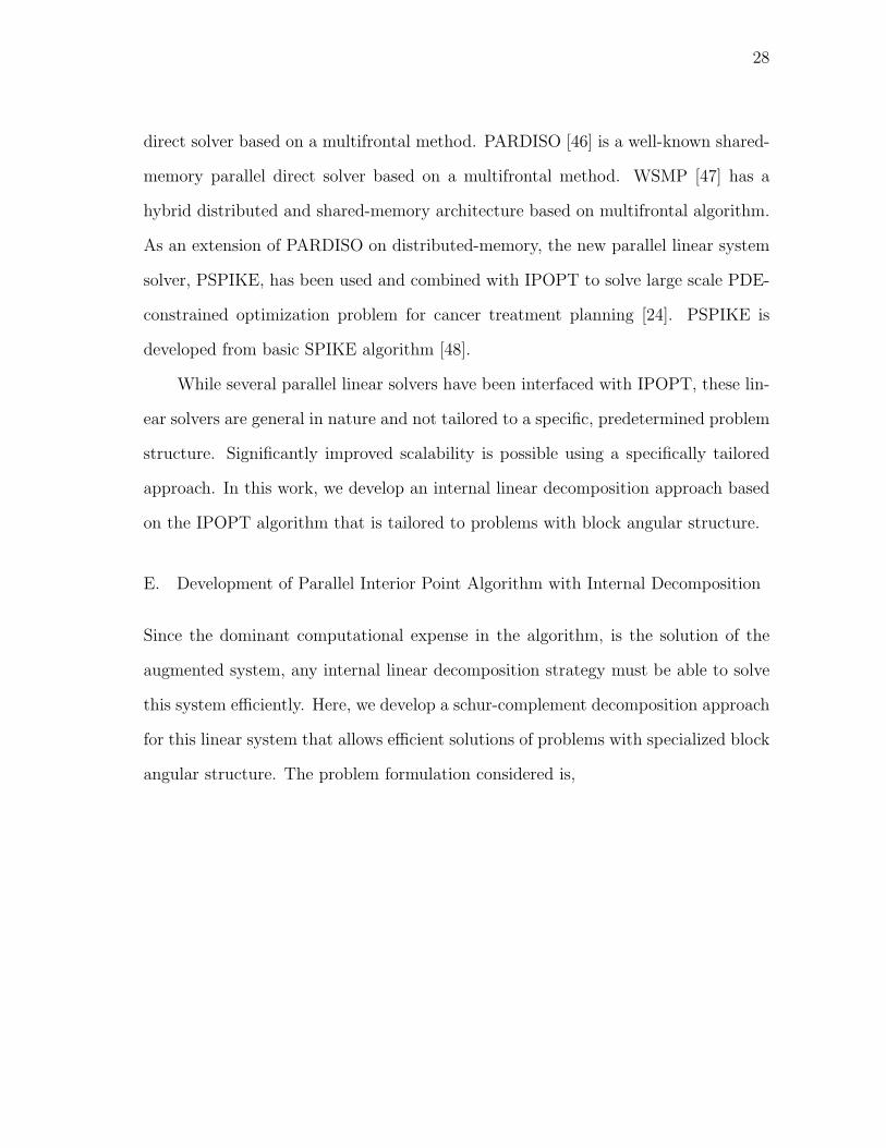
While several parallel linear solvers have been interfaced with IPOPT, these lin-
ear solvers are general in nature and not tailored to a specific, predetermined problem
structure. Significantly improved scalability is possible using a specifically tailored
approach. In this work, we develop an internal linear decomposition approach based
on the IPOPT algorithm that is tailored to problems with block angular structure.
E. Development of Parallel Interior Point Algorithm with Internal Decomposition
Since the dominant computational expense in the algorithm, is the solution of the
augmented system, any internal linear decomposition strategy must be able to solve
this system efficiently. Here, we develop a schur-complement decomposition approach
for this linear system that allows efficient solutions of problems with specialized block
angular structure. The problem formulation considered is,
Page 45
29
minzq ,y
∑q∈Q
Γq (zq)
s.t. Ωq (zq) = 0
ϕLq ≤ (PL
ϕq)Φq (zq)
ϕUq ≥ (PU
ϕq)Φq (zq)
zLq ≤ (PLzq)zq
zUq ≥ (PUzq)zq
Lzqzq − Lyqy = 0 (2.19)
where zq are the all local variables corresponding to block q, and y is a vector of
common variables coupling the blocks. The matrices Lzq and Lyq define the linking
relationship between local variables within each block and the common variables. The
equations Ωq contains all local equality constraints corresponding to block q. Note
that Ωq need not have the same structure in each block. The permutation matrices,
PLϕq, PU
ϕq, PL
zq , PUzq and Φq form the inequality constraints for each block. Note that
common variables, y, are not included in any local equality or inequality constraints.
Rather than deriving the augmented system for this problem formulation, we
simply define the mapping between the problem in Equ. 2.12 and the problem in
Equ. 2.19. The primal variables, and their bounds are given by
x =[z1, . . . , znq , y
]T; (2.20)
xL =[zL1 , . . . , z
Lnq,]T
; (2.21)
xU =[zU1 , . . . , z
Unq,]T
; (2.22)
Page 46
30
with the corresponding permutation matrices,
PLx =
PLz1
0 0 0
0. . . 0
...
0 · · · PLznq
0
(2.23)
PUx =
PUz1
0 0 0
0. . . 0
...
0 · · · PUznq
0
(2.24)
The objective function, equality constraints, inequality constraints, and bounds s
defined as,
f(x) =∑q∈Q
Γq (zq) , (2.25)
c(x) =[Ω1 (z1) , Lz1z1 − Ly1y, · · · , ,Ωnq
(znq
), Lznq
znq − Lynqy]T
, (2.26)
d(x) =[Φ1(z1), . . . , Φznq
(znq)]T
; (2.27)
dL =[ϕL1 , . . . , ϕ
Lnq,]T
; (2.28)
dU =[ϕU1 , . . . , ϕ
Unq,]T
; (2.29)
with the corresponding permutation matrices,
PLd =
PLd1
0 0 0
0. . . 0
...
0 · · · PLdnq
0
(2.30)
PUd =
PUd1
0 0 0
0. . . 0
...
0 · · · PUdnq
0
(2.31)
Using this mapping, the augmented system of Equ. 2.18 can be rearranged to a
Page 47
31
block-bordered structure as,
K1 A1
K2 A2
. . ....
Knq An
AT1 AT
2 · · · ATnq
δ1I
∆t1
∆t2...
∆tnq
∆y
=
r1
r2...
rnq
ry
(2.32)
where
Kq =
Hzq + δ1I · ∇zqΩq LTzq ∇zqΦq
· δ1I · · −I
∇zqΩTq · −δ2I · ·
Lzq · · −δ2I ·
∇zqΦTq −I · · −δ2I
, (2.33)
ATq =
[· · · LT
yq ·], (2.34)
∆tq =[∆zq , ∆sq , ∆λΩq , ∆λLzq
, ∆λΦq
]T, (2.35)
rq =[rzq , rsq , rΩq , rLzq
, rΦq
]T, (2.36)
Given the structure of Equ. (2.32), we can separate the problem by eliminating
each of the AT matrices in the bottom block of rows and solve the linear system with
the schur-complement approach,
[δ1I −
∑q∈Q
ATq K
−1q Aq
]∆y = ry −
∑q∈Q
ATq K
−1q rq (2.37)
Kq∆tq = rq − Aq∆y,∀q ∈ Q. (2.38)
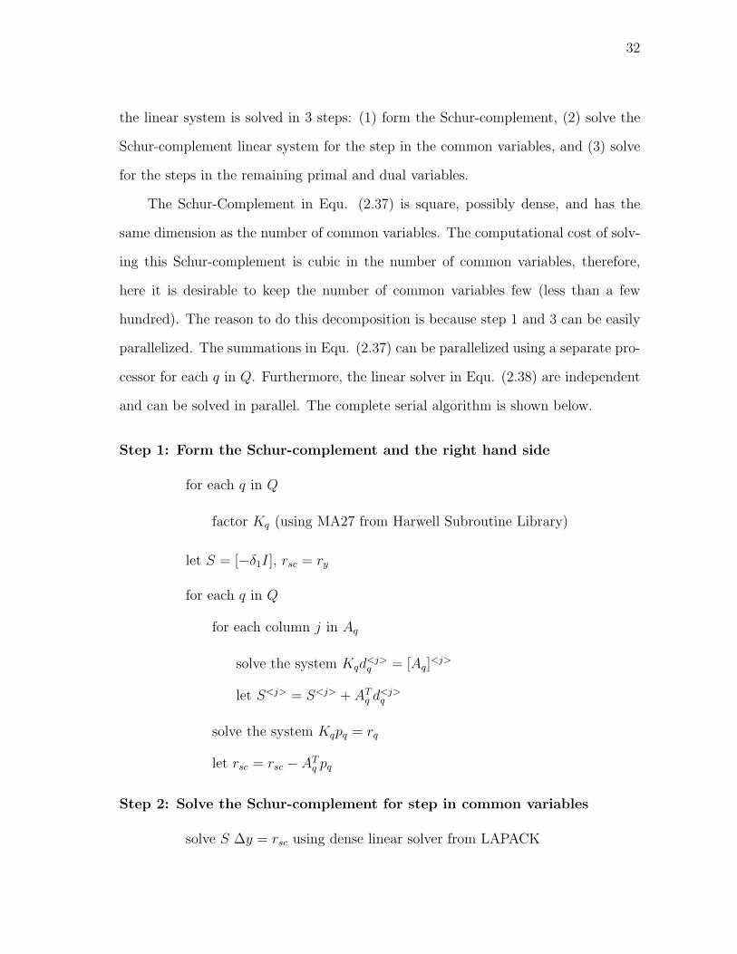
Therefore, instead of solving the complete system with a single direct solver,
Page 48
32
the linear system is solved in 3 steps: (1) form the Schur-complement, (2) solve the
Schur-complement linear system for the step in the common variables, and (3) solve
for the steps in the remaining primal and dual variables.
The Schur-Complement in Equ. (2.37) is square, possibly dense, and has the
same dimension as the number of common variables. The computational cost of solv-
ing this Schur-complement is cubic in the number of common variables, therefore,
here it is desirable to keep the number of common variables few (less than a few
hundred). The reason to do this decomposition is because step 1 and 3 can be easily
parallelized. The summations in Equ. (2.37) can be parallelized using a separate pro-
cessor for each q in Q. Furthermore, the linear solver in Equ. (2.38) are independent
and can be solved in parallel. The complete serial algorithm is shown below.
Step 1: Form the Schur-complement and the right hand side
for each q in Q
factor Kq (using MA27 from Harwell Subroutine Library)
let S = [−δ1I], rsc = ry
for each q in Q
for each column j in Aq
solve the system Kqd<j>q = [Aq]
<j>
let S<j> = S<j> + ATq d
<j>q
solve the system Kqpq = rq
let rsc = rsc − ATq pq
Step 2: Solve the Schur-complement for step in common variables
solve S ∆y = rsc using dense linear solver from LAPACK
Page 49
33
Step 3: Solve for steps in remaining variables
for each q in Q
solve Kq∆tq = rq − Aq∆y for ∆tq
In this algorithm, there are two potential levels of parallelism. On the first level,
each for loop overall q in Q can be parallelized. This requires one processor for each
block in Q. This level of parallelized has been implemented in the work in this dis-
sertation. The second potential for parallelism occurs in step 1. If enough processors
are available, then the for loop over all columns j in Aq can also be parallelized. This
level of parallelism is not implemented in this dissertation.
This section describes the algorithm for parallel solution of the augmented system
since this is the dominant computational expense. Nevertheless, all scale dependent
operations need to be parallelized for an efficient algorithm. This means that all
required linear operations, including all matrix-vector and vector-vector operations
much be parallelized. This is discussed further in the next section.
Our parallel implementation is based on the nonlinear optimization package,
IPOPT. A recent reimplementation of the IPOPT code focused on a design that al-
lows straightforward customization of all the linear operations for structure specific
problems. A high-level illustration of the design is shown in Figure 2. The fundamen-
tal algorithm code is separated from both the problem specification and the details of
the implementation of all linear operations. This means that the algorithm code itself
never accesses individual elements in any matrix or vector, but rather performs all
operations through the base-class interfaces of the linear algebra library. With this
approach the algorithm code is completely independent from the linear solver and
the implementation of the linear operations. This is extremely valuable since custom
linear operations can be developed that exploit the problem structure without any
Page 50
34
necessary changes to the algorithm code itself. Furthermore, all the theoretical bene-
fits of the IPOPT algorithm are retained since the parallel implementation performs
the same mathematical operations - it just performs them more efficiently, in parallel.
Fig. 2. Redesign IPOPT Structure with Specialized NLP and Linear Algebraic Imple-
mentation
In our implementation, the structure of the problem must be specified so it can
be recognized within the linear operations. On the problem formulation side, we
have implemented a composite NLP that forms the block-angular problem from sep-
arate NLP instances. The overall objective function is built up as the summation
of the individual contributions from each of the blocks, and the constraints from
each individual NLP is included as independent blocks in the composite NLP. A
secondary specification is used to describe the linking constraints between the vari-
ables within each block and the common variables. This was a very flexible interface
that allowed straightforward specification of the entire block-angular problem with
individual pieces. Our specific implementation supports the use of individual AMPL
models to represent each block. In parallel, a separate instance of the AMPL Solver
Library (ASL) exists for each block. Therefore, the objective function, constraint
evaluations, and derivatives could all be evaluated in parallel at the block level.
Page 51
35
In addition, a specialized set of linear algebra classes were developed that were
specific to the structure of the block angular problem. This includes both vectors
and matrices. All scale-dependent operations on both the vectors and the matrices
(mat-vec products, dot products, linear solves, etc.) were implemented to allow
parallel solution across individual blocks. Given this approach, it is important to
note that data corresponding to an individual block (all variables, Jacobian, and
Hessian information) is only ever stored with one process. The entire problem never
exists on one machine or needs to be analyzed on one machine. This is a tremendous
benefit that allows parallel solution of very large-scale problems with much improved
scalability. All of the required parallel communication is performed using the MPICH
implementation of the Message Passing Interface (MPI).
The next four chapters of this dissertation address several challenging problems in
chemical engineering. Each of these problem classes is amenable to parallel solution
using the algorithm previously discussed. In each chapter, the rigorous nonlinear
models, problem formulations, and solution results are discussed.
Page 52
36
CHAPTER III
DESIGN UNDER UNCERTAINTY
Design with unknown information is an important problem in chemical process en-
gineering area. As mentioned in the Chapter I, taking uncertain information into
account at the design phase can increase the robust operating performance and pro-
cess flexibility.
To handle potential uncertainties in the design phase, the traditional approach
is to design the process according to nominal values of the uncertain parameters and
then overdesign based on empirical factors. However, this approach may result in
infeasible or conservative design decisions. The development of systematic design
methods that explicitly consider process uncertainty has been an important research
topic for many years [49, 50]. The two dominant approaches for rigorous consider-
ation of uncertainty in optimization are the stochastic programming approach and
the chance-constrained approach. Grossmann and Guillen-Gosalbez [51] recently dis-
cussed the opportunities for the use of these approaches in the syndissertation and
planning of sustainable processes.
In the stochastic programming approach, individual scenarios are included in the
optimization formulation for each discrete realization of the uncertain parameters.
Continuous uncertainty spaces are usually approximated by appropriate sampling.
The problem can be formulated using multiple stages with potential for decisions (or
recourse) at each stage. Several good textbooks describe this approach in detail [52].
In chance-constrained programming, constraints need not be satisfied over the
entire uncertainty space, but instead they are required to be satisfied with a given
probability. While this explicit description is often desirable, these formulations can
be very difficult to solve in the general case.
Page 53
37
In optimal design under uncertainty, multi-scenario programming problem for-
mulations adopted in this work. Compared with chance-constrained programming,
multi-scenario formulations requires feasibility over all discrete scenarios.
A. Multi-scenario Programming Approaches
Multi-scenario optimization is a popular approach for design of chemical processes
under uncertainty. Several researchers have investigated effective formulation and
solution strategies for this class of problems [53, 54, 55, 56, 57, 58, 59, 60, 61], and
several well known reviews are available [62, 63, 64]. Two stages are typically con-
sidered in these formulations: the design stage and the operation stage. Values for
the design variables must be determined, whereas values of the control variables can
be determined during the operational stage when some uncertainties may have been
resolved.
Rooney and Biegler [60] generalize the multi-scenario approach and classify the
uncertainties into process variability and process uncertainty. Process uncertainty
refers to quantities that are unknown at both the design stage and the operation
stage. The design itself should ensure feasibility across these uncertainties. Process
uncertainty includes, for example, unmeasured disturbances and uncertain model pa-
rameters. Process variability refers to quantities that are uncertain at the design stage
but measurable during operation. Process control variables are allowed to change in
order to compensate for this variability. While multi-scenario programming is a pop-
ular approach, challenges still include efficient solution of these large-scale problems,
especially in the general nonlinear case.
The multi-scenario approach is generally viewed as focusing on reliability more
than profitability since it requires feasibility of all scenarios. However, when the
Page 54
38
uncertainty space is continuous, the discrete scenarios represent only a sample of the
continuous space. Recent research has demonstrated that this approach represents an
approximation of the probabilistic approach and, in special cases, rigorous confidence
intervals can be established [65, 66]. These developments, coupled with improvements
in optimization tools and computational capability, serve to increase the importance
of this approach and its practical applicability.
In conceptual design, unknown information can be classified into two categories
[60, 67]. Process uncertainty includes values that are unknown at the design stage
and the operation stage. These include, for example, unmeasured disturbances, and
unknown model parameters. Process variability includes values that are not known
at the design stage, but can be measured during operation. This variation may be
compensated by control variables.
The multi-scenario formulation can be expressed in general form as:
mind,u
f0 (d) +∑k∈K
∑m∈M
ωmkfmk (d, uk, lmk, θνk , θ
um)
s.t. hmk (d, uk, lmk, θνk , θ
um) = 0
gmk (d, uk, lmk, θνk , θ
um) ≤ 0, k ∈ K, m ∈ M (3.1)
Where the design variables are given by d, control variables are given by u, and
the state variables are given by l. Inequality and equality constraints are given by g
and h respectively. In the multi-scenario formulation, the uncertainty space is sepa-
rated into discrete points. The index set K is defined for discrete values of variable
parameters, θν , and the index set M is defined for discrete values of unknown param-
eters, θu. The objective function includes fixed costs related to the design variables
and a weighted sum arising from a quadrature representation of the expected value
of the objective over the uncertainty space. Discretization points are selected for
Page 55
39
this quadrature, however realizations can be added to enforce feasibility at additional
points. This gives a large-scale nonlinear multi-scenario problem with significant cou-
pling or interaction induced by both the control and design variables. We assume
that the control variables u can be used to compensate for measured variable param-
eters, θν , but not the uncertainty associated with unknown parameters, θu. Thus,
the control variables are indexed over k in the multi-scenario design problem, while
the state variables, determined by the equality constraints, are indexed over m and
k. There are two case studies which are investigated for design under uncertainty in
this chapter.
B. Case Study 1: Design under Uncertainty for Cryogenic Air Separation Units
Cryogenic air separation systems are widely utilized for providing significant quanti-
ties of high purity nitrogen, argon, and oxygen products in many industries including
the steel, chemical, refining, semiconductor, and aeronautical industries. Methods
of air separation include cryogenic and non-cryogenic approaches [68]. Although
non-cryogenic processes such as pressure swing adsorption and membrane separation
have become more competitive, cryogenic distillation technology is still the dominant
choice for producing large quantities of very high-purity and liquefied air products
[69]. However, cryogenic air separation is an energy-intensive process consuming large
amounts of electricity to compress air for separation and liquefying gas products. The
industrial gas industry consumed approximately 31,460 million kilowatt hours (over
$ 700 million/year) in the USA in 1998, which accounts 3.5% of the total electricity
purchased by the manufacturing industry [70, 71]. In 2002, the industrial gas industry
consumed approximately 35,000 million kilowatt hours of electricity in the USA [72],
which is an increase of 11.3% compared with the amount in 1998.
Page 56
40
1. Current Research about Air Separation Systems
Optimizing the design of the cryogenic air separation system has the potential to
significantly affect not only the capital investment, but also the future economic
performance. In practice, most current design schemes focus on specialized column
structures and opportunities for energy and mass integration. Agrawal and cowork-
ers simulate and analyze various thermal coupling methods [73], structured packing
on packed columns for argon production [74], and multiple component distillation
sequences [75, 76] in order to improve energy efficiency and separation performance.
Egoshi, Kawakami, and Asano [77] address the problem of predicting practical sep-
aration performance and obtaining the optimal design of cryogenic air separation
plants using a rigorous transport model for structured packing. Regardless of the
design strategy used, in order to retain future process flexibility it is important to
consider potential uncertainties during the design phase. These include uncertainty
in process performance, uncertainty in product demands and pricing, and uncertainty
in availability and pricing of process inputs.
In addition to design problems, current research on cryogenic air separation
columns includes process optimization and control. Here, we briefly review the rel-
ative literature. Optimization of cryogenic air separation systems also includes high
level planning and scheduling. Dynamic optimization strategies, linear model predic-
tive control, and nonlinear model predictive control techniques have all been applied
to cryogenic air separation systems [78, 79, 80, 81, 82, 83, 84, 79, 85]. These studies
have focused primarily on the use of rigorous models for improving controller perfor-
mance, and on determining optimal operating profiles targeting specific load changes.
However, formulations like these, with detailed process models, typically do not con-
sider high level operating concerns like uncertainty in product demands. On the other
Page 57
41
hand, planning and scheduling studies [86, 87, 88, 71, 89] do consider market uncer-
tainty and product inventory when planning operating strategies. To enable efficient
solution of these challenging problems, simplified or linearized models are often used,
which may ignore the integrated nature of the system and the nonlinear interactions
between multiple products.
In the following chapters, we investigate optimization and control under uncer-
tainty of cryogenic air separation columns. In this chapter, we discuss the design
of integrated air separation units considering both process uncertainty and process
variability.
2. Uncertainties in Air Separation Process
There are several uncertainties affecting optimal solutions of design and operating
problems. One example of uncertainty in the model arises in the selection of ther-
modynamic methods and parameters. The primary components are separated under
extremely low temperatures, and standard packages may not adequately describe the
behavior of the system under these conditions. Indeed, many companies specializing
in air separation have spent significant resources developing specialized thermody-
namic methods for their systems.
A second form of uncertainty relates to unknown demands on the process. Air
separation systems can produce three component products of various grades in both
vapor and liquid phases. Different customers have different product and purity de-
mands, and these demands can change with seasons and other external factors. It is
important to consider this product demand uncertainty during the design phase and
develop a process that is flexible enough to meet future product demands.
A third form of uncertainty comes from unknown or varying availability of process
inputs and pricing. The dominant operating expense in cryogenic air separation
Page 58
42
systems is the electricity required by the process. Peak versus off-peak costs and
real-time pricing changes, can significantly affect the economic performance of the
process. This uncertainty is well studied in a number of articles [87, 71, 89].
3. Process Description
Considering cryogenic air separation systems, uncertainty can arise from several
sources. Process uncertainty (which is unknown during operation) can arise from
unknown physical properties. For example, activity coefficient models for N2–Ar–O2
systems contain binary interaction parameters that are sensitive to argon purities
and pressures [90]. Process variability (or measurable uncertainty) can arise because
of changing product demands. In order to satisfy variable product demands, the
cryogenic air separation system may be required to switch among different operating
conditions. The argon product variability is often ignored; however, it can affect the
optimal design significantly.
A typical cryogenic air separation system includes a double-effect heat integrated
distillation column with a side column of crude argon. The double distillation column
is the common part of all cryogenic air separation systems, while a crude argon
column (CAC) is adopted in some systems for coproduction of argon. Addition of the
argon column increases the complexity of the system significantly through additional
coupling and recycling, and makes operation more difficult than the system with a
double-effect distillation column alone. Figure 3 shows the process flowsheet for the
system studied in this paper. The crude air feed stream is compressed and primary
impurities such as water and carbon dioxide are removed. After cooling, a portion
of the air feed stream is expanded and introduced into the low-pressure distillation
column (LPC) containing 70 theoretical stages. The remaining feed air stream enters
the bottom of the high-pressure distillation column (HPC) with 36 theoretical stages.
Page 59
43
Fig. 3. Simplified Structure of the Cryogenic Air Separation Process
In the combined condenser/reboiler, the partially liquefied stream in the bottom of
the LPC is vaporized, while the nitrogen vapor stream in the top of the HPC is
condensed. A liquid nitrogen stream from the top of the HPC is introduced into the
top of the LPC as the reflux stream. A portion of the oxygen-rich liquid from the
bottom of the HPC is introduced into the 17th tray of the LPC in order to produce
oxygen product with high purity. The remainder of the oxygen-rich liquid is used by
the condenser at the top of the CAC to condense the argon-rich stream and produce
the reflux for the CAC. A side vapor stream primarily composed of oxygen and argon
is withdrawn at the 28th tray of the LPC and separated in the CAC. Liquid oxygen
product is directly taken from combined condenser/reboiler and gas oxygen product
is taken from the bottom of the LPC. Liquid nitrogen product is taken from the top
of the HPC while gas nitrogen product is from the top of LPC. Crude argon product
Page 60
44
is withdrawn from the top of CAC.
This is a highly integrated system that can be very difficult to design and operate.
Typically, there are a large number of design variables which need to be determined
in the detailed design phase of a cryogenic air separation plant. However, this study
mainly focuses on conceptual design under uncertainty. Therefore all valves are as-
sumed to be throttle expansion valves, the mass loss in pipelines are assumed to
be negligible, and constant heat transfer area and coefficients are used in the heat
exchanger calculations. Based on process dynamics of the cryogenic air separation
system, five main control variables, u = [U1, U2, U3, U4, U5], are selected to compen-
sate for variability of argon product demands. These variables are defined as the feed
air stream of the HPC (U1), the feed air stream of the LPC (U2), the reflux flow from
the HPC to the LPC (U3), the waste nitrogen stream (U4), and the side withdrawal
from the LPC to the CAC (U5). The five main design variables are the diameters of
the three distillation columns (the HPC, LPC and CAC), the heat transfer area of
the combined condenser/reboiler, and the brake horsepower of the compressor. Table
I shows the nominal operating conditions of the plant used in the case study.
4. Mathematical Steady State Model of Air Separation Columns
The detailed air separation model is derived using the following four assumptions: (1)
complete mixing on each tray and 100% tray efficiency; (2) negligible heat losses in the
tray; (3) constant pressure drop on each tray; (4) uniform pressure and temperature
on each tray.
The model includes mathematical expressions for the three distillation columns,
two main heat exchangers, two integrated exchangers (one between the HPC and
the LPC, another between the CAC and the HPC), and several throttle valves. The
model contains mass and energy balances for all the exchangers and throttle valves.
Page 61
45
Table I. Nominal Operating Conditions for Design of the Air Separation Unit
Process variable Values
Gas oxygen product, mol/s 2.44
Liquid oxygen product, mol/s 0.64
Oxygen product purity ≥98%
Gas nitrogen product, mol/s 13.13
Nitrogen product purity ≥99.99%
Argon product purity ≥96%
Pressure of the LPC, MPa 0.13-0.14
Pressure of the HPC, MPa 0.68-0.69
Pressure of the CAC, MPa 0.12-0.13
We assume that there is no energy loss in the exchangers, and that the pressure
drops are constant across these units. The three distillation columns are all modeled
using the following tray-by-tray equations, physical property expressions, and phase
equilibrium.
The mass balances for each tray are given by,
F Vj + FL
j + Vj+1 + Lj−1 − Vj − SVj − Lj − SL
j = 0, (3.2)
where j is the index of each tray from the top of each column. F Vj and FL
j are the
vapor and liquid molar feed flows entering into the jth tray. SVj and SL
j are the vapor
and liquid molar side flows out of the jth tray. The vapor and liquid flow rates are
given by Vj and Lj, respectively. Component mass balances are given by,
Vj+1yi,j+1 + Lj−1xi,j−1 + F Vj zVi,j + FL
j zLi,j
−(Vj + SV
j
)yi,j −
(Lj + SL
j
)xi,j = 0 (3.3)
Page 62
46
where i ∈ CP is the index of each component(1-Nitrogen, 2-Argon, 3-Oxygen), the
liquid and vapor compositions are given by xi,j and yi,j respectively. zVi,j and zLi,j are
the vapor and liquid compositions of feed flows entering the jth tray.
The model includes tray by tray energy balances, expressed by,
Vj+1HVj+1 + Lj−1H
Lj−1 + F V
j HFVj + FL
j HFLj
−(Vj + SV
j
)HV
j −(Lj + SL
j
)HL
j = 0, (3.4)
where HFVj and HFL
j are the vapor and liquid enthalpies of feed flows entering into
the jth tray. The vapor and liquid enthalpies of the jth tray are given by HVj and HL
j
respectively. HFVi,j , HFL
i,j , HVi,j and HL
i,j are calculated by,
HVj =
∑i∈CP
yi,jHVi,j (Tj,Pj) + ∆HV
mix (Tj,Pj) (3.5)
HLj =
∑i∈CP
xi,jHLi,j (Tj,Pj) + ∆HL
mix (Tj,Pj) (3.6)
HFVj =
∑i∈CP
yi,jHFVi,j
(T Fj ,PF
j
)+∆HFV
mix
(T Fj ,PF
j
)(3.7)
HFLj =
∑i∈CP
xi,jHFLi,j
(T Fj ,PF
j
)+∆HFL
mix
(T Fj ,PF
j
)(3.8)
where HFVi,j , HFL
i,j , HVi,j and HL
i,j are the vapor and liquid enthalpies of each component
in each tray respectively, while these enthalpies are calculated based on relevant
bubble point temperatures (T ) and pressures (P). ∆Hmix is mixture enthalpies and
calculated with relevant compressibility factors and binary interactive parameters.
The temperature and pressure dependence of the enthalpies were represented using a
high-order polynomial fit to simulation data.
Summation equations in the jth tray are written by
∑i∈CP
yi,j = 1 (3.9)
Page 63
47
The vapor-liquid equilibrium expressions for each tray are given by,
yi,j = κjγjKi,jxi,j + (1− κj) yi,j+1 (3.10)
where κj is the Murphee tray efficiency of the jth tray, K is the ideal vapor-liquid
equilibrium constant calculated using Antoine equations (3.12) and γ is the activ-
ity coefficient calculated with Margules equations (3.13-3.15). The tray efficiency is
assumed to be 100% in this study, giving (3.11) from (3.10).
yi,j = γjKi,jxi,j (3.11)
Ki,j = exp [Ai − (Bi/ (Tj + Ci))]/Pj (3.12)
log γ1,j =
(A1,3x
23,j + A1,2x
22,j + (A1,3 + A1,2 − A2,3) x3,jx2,j
RTj
)(3.13)
log γ2,j =
(A1,2x
21,j + A2,3x
23,j + (A1,2 + A2,3 − A1,3) x1,jx3,j
RTj
)(3.14)
log γ3,j =
(A1,3x
21,j + A2,3x
22,j + (A1,3 + A2,3 − A1,2) x1,jx2,j
RTj
)(3.15)
where R is the ideal gas constant and Margules constants, ai,k describe the liquid
phase interactions between components i and k. Margules constants can be found in
[90] while Antoine constants are reported in http://webbook.nist.gov/chemistry/.
The combined condenser/reboiler is modeled as an additional normal tray for
both the HPC and the LPC, which is given by (3.16).
Q1 = UA1
(THPC1 − TLPC
70
)= V HPC
1
(HV,HPC
1 −HL,HPC1
)=
(V LPC70 + SV
70
) (HV,LPC
70 −HL,LPC70
)(3.16)
where Q1 is the energy transfer from the HPC to the LPC. UA1 is the heat transfer
coefficients in the condenser/reboiler. THPC1 is the temperature at the first tray of
the HPC and TLPC70 is the temperature at the last tray of the LPC. V HPC
1 is the vapor
Page 64
48
flow of the first tray in the HPC, which is fully condensed by Q1. The heat Q1 is
released to the vapor flow V LPC70 and oxygen product flow SV
70 at the last tray of the
LPC.
Similarly, the heat-integrated condenser of the CAC is modeled using (3.17). The
energy, Q2, is extracted from the condensing vapor stream at the top of the CAC and
released to a portion of the liquid oxygen-rich stream so that this stream is partially
vaporized.
Q2 = UA2
(TCAC1 − TO2−rich
)= V CAC
1
(HV,CAC
1 −HL,CAC1
)= ∆VO2−rich
(HV
O2−rich−HL
O2−rich
)(3.17)
where TCAC1 , HV,CAC
1 and HL,CAC1 are the temperature, vapor and liquid enthalpies at
the first tray of the CAC, respectively. V CAC1 is the vapor flow at the first tray of the
CAC. TO2−richand ∆VO2−rich
are temperature and the partially vaporized amount in
the oxygen-rivh stream, respectively. HVO2−rich
and HLO2−rich
are the vapor and liquid
enthalpies for vaporization in the oxygen-rich stream.
5. Mathematical Formulation for Conceptual Design under Uncertainty
The following expressions are used to capture design relationships [91, 92]. Column
diameters are given by,
Dm,j =
(0.0164V 0.5
m,j
[378Mg
(Tm,j
520
)(14.7
Pm,j
)] 14
)(3.18)
where Pm is the tray pressure of each column, and Mg is the molecular weight of
distillate.
Dm = max(Dm,j),m ∈ (LPC,HPC,CAC) (3.19)
Page 65
49
The height of each column is,
Hm = 2.4nm, (3.20)
where nm is the number of stages in each column and the heat transfer area in the
combined condenser/reboiler can be described by,
A =Q
U∆T, (3.21)
where ∆T is the temperature driving force. QI is the transferred heat between the
LPC and the HPC, and U is the heat transfer coefficient. The capital costs of column
shells and trays (CSC and CTC) are estimated with the following equations:
CSCm =
(M&S
280
)102D1.066H0.802 (cin + cmcp) (3.22)
CTCm =
(M&S
280
)4.7D1.55H (cs + ct + cm) (3.23)
Here, M&S is the Marshall and Swift index. The parameters cp, cm and cin are the
pressure range, construction material and installation cost coefficients. The param-
eters cs and ct are the tray spacing and design cost coefficients, respectively. The
capital cost of heat exchanger (HEC) in combined condenser/reboiler is,
HEC =
(M&S
280
)102A0.65 (cin + cm (ct + cp)) (3.24)
and the capital cost of the main compressor (CPC) is,
BHP =
((U1 + U2)
1−∆Fl
κ
κ− 1RTin
((Pout
Pin
)κ−1κ
− 1
))(3.25)
CPC =
(M&S
280
)518 (BHP )0.82 (cin + ct) (3.26)
where BHP is the brake horsepower of the compressor. The entrance and exit pres-
sures of the compressor are Pin and Pout, and ∆Fl is the loss amount of the feed flow
Page 66
50
in the compressor. The adiabatic index number of the gas is given by k.
Because the major operating cost of cryogenic air separation processes is required
electrical power, we assume the other operating costs can be ignored. Here, we also
assume that a liquefier is not installed in the system. The power price is assumed to
be constant in this study, however, more complex formulations considering uncertain
power prices will be investigated in future work.
The electricity cost (EC) is given by,
EC = CeleBHP
η(3.27)
where Cele is electricity price ($0.0574/(kWh)), and η is the efficiency of the compres-
sor (0.75). The total annual cost (TAC) of our air separation process is given by the
following form,
TAC =(CSC + CTC +HEC + CPC)
tp+∑k∈K
∑q∈Q
(ωqkECqk) (3.28)
where tp is the payback time, which is assumed to be 3 years. The last term in
Eq. (3.28) is a numerical integration for the expected value of the operating cost.
In the case studies, we assume that variability and uncertainty are both uniformly
distributed. Therefore, the weights ωqk are all equal. More accurate quadrature rules
could be used along with other distributions. Other costs such as pipelines and valves
are not included in this study.
6. Numerical Results
The base formulation described in the previous subsection is used to find the optimal
design for the nominal case. In addition, a multi-scenario formulation is developed
Page 67
51
Fig. 4. Timing Results for Multi-Scenario Approach (Default options)
that considers uncertainty in argon product demands and the thermodynamic param-
eter α12, and evaluates the objective using the expected value of the operating costs.
Before discussing the optimization results in detail, we first present the timing results
showing the scalability of the multi-scenario approach with IPOPT.
Argon product demands are assumed to be uniformly distributed between 0.1063
(-20%) mol/s and 0.1595 (+20%) mol/s, and the binary interaction parameter, α12,
is assumed to be uniformly distributed between 7.0 and 9.5. Figure 4 shows the
IPOPT solution times using the default options. The same number of discretizations
is used for each uncertain parameter, and the category labels give the total number
of scenarios considered for each run. The white bars on the left list the average CPU
time for each iteration. The grey bars on the right list the total CPU time in seconds.
Note that the number of iterations need not be the same for each case. Furthermore,
by default IPOPT uses exact first and second derivative information, and the number
Page 68
52
Fig. 5. Timing Results for Multi-Scenario Approach (L-BFGS)
of iterations remains relatively constant as the size of the problem increases.
Figure 5 shows the timing information using the quasi-Newton approach within
IPOPT. With this option, the Hessian information is approximated using a limited
memory BFGS update. Similar scaling is seen for this approach. The number of
variables in the 4 scenario case is approximately 8,000, while the number of variables
in the 196 scenario case is approximately 675,000. These results demonstrate that
off-the-shelf nonlinear programming tools are able to scale effectively to reasonably
large problems, even when the models are highly coupled and nonlinear.
Taking the largest number of scenarios (196 scenarios), optimal results from the
multi-scenario formulations are compared with optimal results for the nominal case in
Table II. As expected, the design is more conservative when uncertainty is considered.
The optimal diameter of the HPC is the least sensitive to the uncertainty considered
here.
The diameter of the CAC and the brake horsepower are significantly affected.
Page 69
53
Table II. Optimal Design for the Nominal and Multi-scenario Formulation of the Air
Separation Unit
Variables Nominal Case Multi-scenario Case Difference
Diameter of LPC (m) 0.66 0.76 15.65%
Diameter of HPC (m) 0.88 0.95 8.24%
Diameter of CAC (m) 0.44 0.54 23.42%
BHP (KW) 90 113 25.57%
Heat exchanger area (m2) 24 26 11.45%
TAC ($106) 1.412 1.586 12.35%
This is reasonable, since the variability in argon demands will require greater process
flexibility. This result also shows that it is not optimal (and may not be feasible)
to absorb potential argon variability by operational changes alone. Both design and
operation changes should be considered. The effects of these uncertainties on the
diameter of the LPC are more dramatic than on the diameter of the HPC. This
is expected given the variability in argon production and the integration between
the LPC and the CAC. Increased withdrawal from the LPC to the CAC, coupled
with variability in recycle from the CAC, requires increased flexibility in the LPC. In
contrast, the CAC is less tightly integrated with the HPC.
Figure 6 shows how the optimal design changes as a function of the number
of scenarios considered. The values for the argon demand and the uncertain binary
interaction parameter were selected randomly from the ranges given previously. While
it is difficult to guarantee that the scenarios sufficiently span the space of variability
and uncertainty, it can be seen that the multi-scenario design solution converges as
we increase the number of scenarios.
Page 70
54
Fig. 6. Dependence between Multi-scenario Design and Increasing Scenario Number
7. Conclusions and Future Work
a. Summary and Conclusions
This work uses a multi-scenario approach to determine the optimal design of a cryo-
genic air separation process considering two classes of uncertainty. Process variability
is describes uncertainty that is measurable during operation, and control variables can
be used to compensate for this uncertainty. Process uncertainty represents unmea-
surable quantities like uncertain model parameters or unmeasured disturbances. In
this paper, argon product demands were selected as an example of process variability,
and unknown activity coefficients were selected as an example of process uncertainty.
As expected, the optimal design is more conservative when uncertainties are con-
sidered. However, the multi-scenario approach provides a more rigorous treatment of
uncertainty than applying traditional overdesign factors. The approach allows for a
Page 71
55
more efficient design by capturing the potential for operational changes in the control
variables as a function of process variability. Furthermore, nonlinear interactions be-
tween the uncertainties, the design decisions, and these potential control possibilities
are rigorously captured.
While multi-scenario programming is a popular approach for treatment of un-
certainty in optimization, it can be challenging to find efficient solution strategies
for these large-scale problems, especially in the general nonlinear case. Neverthe-
less, there have been significant advancements in nonlinear programming algorithms,
and the capabilities of general off-the-shelf solvers (e.g. IPOPT) have increased dra-
matically. The largest multi-scenario problem considered in this paper includes 196
scenarios and more than 675,000 variables. Nevertheless, this formulation solves in
under 20 minutes on a standard desktop computer. These results show that recent al-
gorithm improvements, coupled with continued increases in computational capability,
allow practical application of the multi-scenario approach with rigorous, large-scale
nonlinear models. This will be even more evident as we continue to develop algo-
rithms that can exploit modern computing architectures to promote efficient solution
in parallel.
b. Future Work
In this study, a rigorous model of an air separation process was developed that con-
sidered three highly integrated columns. The two uncertainties considered were a
thermodynamic interaction parameter and the argon product demand. Future work
is needed to include treatment of additional uncertainties. A key variability during
operation is the price of electricity, which is the dominant operating cost for the pro-
cess. A careful analysis will help engineers further quantify the impact of this and
other uncertainties on design and operation.
Page 72
56
This work used a steady-state model and assumed that perfect control was pos-
sible. Given the potential control challenges with such a highly integrated process,
these optimization formulations should consider integrated design and control.
Finally, the main challenge in multi-scenario optimization is still efficient solu-
tion of the large-scale problem. The dominant computational expense of the IPOPT
algorithm is the solution of the augmented linear system resulting from a Newton
iteration of the primal-dual equations. Given a problem with a specialized struc-
ture, decompositions are possible that can exploit this structure and produce efficient
solutions in parallel. We have developed a package, SCHUR-IPOPT, that uses an
internal decomposition approach for the parallel solution of structured nonlinear pro-
gramming problems based on the serial IPOPT algorithm. For the general design
under uncertainty formulation, previous results on a large distributed cluster have
demonstrated that the solution time is almost constant as scenarios and processors
are added [93, 39, 85]. In the general multi-scenario formulation considering both pro-
cess variability and process uncertainty, there is additional structure. If the problem
is decomposed with a single scenario for each processor, then the common variables
in the parallel decomposition include both the control variables and the design vari-
ables. However, there is no restriction that each individual block needs to consider
only a single scenario. If the problem is decomposed over the process variabilities
only, then the number of common variables considered in the parallel decomposition
includes only the design variables. With this scheme, the coupling induced by the
control variables is handled internally by the serial linear solver. Furthermore, nested
decomposition strategies are possible to promote further parallelization. Future work
will include the development of specialized decomposition strategies for this nested
structure.
Page 73
57
C. Case Study 2: Design under Uncertainty for Internal Heat-integrated Distillation
Columns
1. Process Description
In this subsection, we determine optimal design solutions under uncertainty with con-
sideration of controllability for an internal heat-integrated distillation column. Here,
on schur-complement decomposition approach is used for parallel solution. Internal
heat-integrated distillation column has received increased attention in recent years due
to its high efficiency and potential for energy saving [94, 95, 96, 97, 98, 99, 100, 101].
Figure 7 shows the structure of this process. The rectifying section and the strip-
ping section in this process are separated into two columns operating at the different
pressures. To adjust the pressures, a compressor and a throttling valve are installed
between the two sections. Unlike the case of the conventional columns, the con-
denser and reboiler are not required in this process. Most previous research on this
Fig. 7. Simplified Structure of Internal Heat-integrated Distillation Column
process focuses on two areas: conceptual design [95, 97, 98, 99] and dynamic con-
Page 74
58
trol [97, 100, 101]. However, little existing research in this area considers potential
uncertainties during the design phase. Adopting deterministic values of operating
parameters without considering the impact from unknown information may produce
a design that does not perform as expected. Conceptual design under uncertainty
can provide more reliable performance in practical scaleup processes, compared to
nominal design parameters that do not consider uncertainty.
2. Mathematical Model of the Process
In order to minimize the total annual cost, a rigorous mathematical model of internal
heat-integrated distillation column is built in the modelling language, AMPL, based
on the mass and energy balances coupled with the equilibrium relationships. The
number of total trays and the feed tray are fixed to 30 and 16, respectively, while the
stripping section pressure is assumed to be 0.1013MPa. Detailed model information
can be found in references [94, 96].
0 = V2Y2 − V1Y1 − L1X1 (3.29)
0 = Vj+1Yj+1 − VjYj + Lj−1Xj−1 − LjXj, j = 2, .., n− 1 and j = f (3.30)
0 = Vf+1Yf+1 − VfYf + Lf−1Xf−1 − LfXf + FZf (3.31)
0 = −VnYn + Ln−1Xn−1 − LnXn (3.32)
0 = Lj −j∑
k=1
Qk/λ, j = 1, .., f − 1 (3.33)
0 = Lf+j−1 − Lf−1 − Fq + Lj, j = 1, .., f − 2 (3.34)
0 = Ln − F − V1 (3.35)
0 = V1 − F (1− q) (3.36)
0 = Vj+1 − V1 − Lj, j = 1, .., f − 1 (3.37)
Page 75
59
0 = Vf+j − Vf + F (1− q)− Lj, j = 1, .., f − 2 (3.38)
0 = Yj − αXj((α− 1)Xj + 1)−1 (3.39)
0 = Qj − UA (Tj − Tj+f−1) , j = 1, .., f − 1 (3.40)
0 = Tj − b/(a− log
(P satj
))+ c (3.41)
0 = P satj − P (Xj − (1−Xj) /α)
−1 (3.42)
where V and L are vapor and liquid flow rates; T , P , and F are temperature, pressure,
and feed flow rate; X and Y are the mole fraction of the liquid and vapor in each
tray; f is the feed tray, and Q is the heat transfer amount of each tray. UA is the
heat transfer rate and α is the relative volatility. The variables q and Zf are the feed
thermal condition and mole fraction of the feed respectively, and n is the number of
total trays indexed by j. Pr is pressure of the rectifying section.
In addition, some inequality constraints are given by,
V1Y1 − FZf ≤ 0 (3.43)
Y1 ≥ 97% (3.44)
Xn ≤ 4% (3.45)
0.1013Mpa ≤ Pr ≤ 0.7091Mpa (3.46)
0 ≤ q,Xj, Yj ≤ 1 (3.47)
Page 76
60
a. Conceptual Design Formulation
The design formulas for installation and operating cost are given briefly and detailed
information can be found in references [99, 97, 91, 92].
D = max
(0.0164V 0.5
j
[379MG,j
(Tb,j
520
)(14.7
PT,j
)] 14
)(3.48)
H = 2.4n (3.49)
A =Q
U∆T(3.50)
CSC =
(M&S
280
)102D1.066H0.802 (cin + cmcp) (3.51)
CTC =
(M&S
280
)4.7D1.55H (cs + ct + cm) (3.52)
HEC =
(M&S
280
)102A0.65 (cin + cm (ct + cp)) (3.53)
BHP =
(F
1−∆Fl
κ
κ− 1RTin
((Pout
Pin
)κ−1κ
− 1
))(3.54)
CPC =
(M&S
280
)518 (BHP )0.82 (cin + ct) (3.55)
EC = CeleBHP
η(3.56)
TAC =(CSC + CTC +HEC + CPC)
tp+∑k∈K
∑m∈M
(ωmkECmk) (3.57)
where D are the diameters of the distillation column, H are the heights of the distil-
lation columns, A is the heat transfer area, and ∆T is the temperature driving force.
The capital costs of column shells and trays as estimated are given by CSC and
CTC, respectively. The cp, cm, and cin are the pressure range, construction material,
and installation cost coefficients. The variables cs and ct are the tray spacing, and
design cost coefficients. The capital costs of heat exchanger and a main compressor
Page 77
61
are given by HEC and CPC, respectively. The major operating cost is given by EC.
Cele is electricity price and η is the efficiency of the compressor. The total annual
cost, (TAC), is minimized in our optimization problem.
The three main design variables selected include: the diameter of distillation
columns, D, the heat transfer area, UA, and the brake horsepower, BHP . Again,
two types of uncertainty are considered in this work, unmeasurable and measurable
uncertainty. The relative volatility of benzene and toluene, which may vary from
2.517 to 2.117 is selected as an unmeasurable uncertainty. The range is discretized by
selecting 7 points assuming a normal distribution. Measurable uncertainties include
the concentration of the feed flow, Zf , which varies from 0.55 to 0.45, and the feed
flow rate, F , which varies from 90 to 110 (mol/s). Both of them are measurable
during operation and may be compensated by two control variables: the rectifying
section pressure, Pr, and the thermal condition in the feed flow, q. Here, we dis-
cretize the uncertainty in Zf and F by selecting 15 points with normally distributed
assumptions. In this large-scale structured problem, there are 1575 scenarios and
approximately 300, 000 total variables including 453 common variables (the design
and control variables common across the scenarios).
3. Controllability Constraints
In the previous subsection, it is assumed that the control variables are able to compen-
sate process variability caused from the measurable uncertainties Zf and F . However,
the above assumption is not easily satisfied. Inherent conflicts between process de-
sign and control are present in a lot of chemical processes. The design solution that
results in challenging control problems should be avoided even if this design provides
low capital and operating cost. Therefore, this work considers controllability con-
straints on the conceptual design in order to avoid potential serious control problems.
Page 78
62
Here, we only select the rectifying section pressure, Pr, and thermal condition in the
feed flow, q as control variables to reject disturbances from both mole fraction of feed
flow and feed flow rate, based on our previous dynamics research [100, 101]. The work
does not attempt to test all potential control pairings. A relative gain array (RGA)
is employed for interaction analysis. The 2× 2 RGA matrix is defined by:
RGA =
λ11 1− λ11
1− λ11 λ11
(3.58)
The RGA value λ11 of the internal heat integrated distillation column is limited
greater than 0.65, to avoid difficult control interactions during dynamic operation. In
addition to RGA, the condition number (γ) is also adopted here as an index of loop
interaction, which is the ratio between the maximum singular value (σmax) and the
minimum singular value (σmin) of the process shown in 3.59. The condition number
of internal heat integrated distillation column is limited to be less than 9.
γ = σmax/σmin (3.59)
4. Optimal Results
The objective function of the above problem focuses on how to minimize the total
annual cost. In order to obtain comprehensive design information, the results with
and without uncertain parameters and controllability, are compared and listed in the
Table III. As expected consideration o uncertainty and controllability leads to more
conservative designs.
To demonstrate the scaleup properties of Schur-IPOPT on a multi-core parallel
machine, we solve problems with an increasing number of scenarios (225 scenarios
for each block). The timing results are shown in Figure 8. With each additional
Page 79
63
Table III. Design Results with/without Considering Uncertainties and Controllability
(HIDiC)
Variables Nominal Case Multi-scenario Case difference
Diameter, ft 2.1 3.0 42.8%
Horsepower, KW 22.5 39.4 75.1%
Heat exchanger area, ft2 210 245 16.7%
block, we utilize an additional processor. These results show that there is significant
performance improvement possible with the parallel approach. Furthermore, this
approach scales favourably as we increase the number of processors used. These
results were obtained on an 8-core, 3.2Ghz Intel Xeon architecture.
We also tested the scalability of our approach against the general purpose, shared-
memory linear solver PARDISO [46]. We do not have a version of the solver interfaced
with the IPOPT. Therefore, to compare the computational time for PARDISO to per-
form the numerical factorization and backsolve of the same linear system arising from
a particular iteration of the Schur-IPOPT solver is measured. It is important to note
that PARDISO performs a symbolic factorization prior to performing the numerical
factorization. However, within an optimization context, the symbolic factorization
would only need to be performed once, at the beginning of the optimization, there-
fore this time was not included in the results. For this reason, coupled with the fact
that PARDISO is simply solving the linear system and not performing the other se-
rial operations required by Schur-IPOPT, the comparison is conservative (that is the
comparison favors PARDISO somewhat). Figure 8 and Figure 9 show the normalized
wall clock time for the two techniques. The x-axis shows the number of blocks, with
an additional thread or process added along with each block.
Page 80
64
Fig. 8. Parallel Scalability Results of Schur-IPOPT on a Multi-core System
We can see that, in both cases, the scalability as we increase the size of the
problem is impressive. We see a slight increase in the wall clock time as we increase the
size of the problem, which is primarily due to memory bandwidth issues. The Schur-
IPOPT approach does scale better than the general purpose solver PARDISO due
to the fact that it is tailored to the specific problem structure. Furthermore, Schur-
IPOPT shows even better scalability on distributed architectures to many processors,
whereas PARDISO is available for shared-memory machines only.
Page 81
65
Fig. 9. Parallel Scalability Results of PARDISO on a Multi-core System
Page 82
66
CHAPTER IV
OPTIMAL OPERATION: UNCERTAIN DEMANDS AND CONTRACTUAL
CONSTRAINTS
In Chapter III, optimal design under uncertainty is studied for cryogenic air separation
columns and internal hear-integrated distillation columns. In this chapter, we instead
focus on optimal operation under uncertainty. Specially, we address optimal operation
of cryogenic air separation processes with uncertain product demands and constraints
on customer satisfaction levels.
A. Previous and Proposed Research on Operation of Air Separation Units
Optimal operation and control of cryogenic air separation processes has received sig-
nificant attention, with the primary goal of reducing energy consumption and im-
proving economic performance during operation. Load switching in air separation
columns are analyzed by [78], and multivariable control schemes for cryogenic air
separation are developed in [79] and [80]. Trierweiler and Engell [81] investigated
the selection of an appropriate control structure based on dynamic behavior analysis.
Seliger, Hanke, Hannemann, and Sundmacher [82] integrated an air separation pro-
cess model with an IGCC power plant and analyzed the combined process dynamics.
Control strategies such as nonlinear model predictive control (NMPC) are difficult to
implement for these systems because of the high computational cost associated with
optimization of a large, complex dynamic model. Approaches have been developed
that promote efficient NMPC for these systems by reducing the size and complex-
ity of the model. Bian, Henson, Belanger, and Megan [83] developed a strategy for
nonlinear model predictive control by adopting a dynamic wave model for the single
nitrogen column. The advanced step NMPC controller [102], an alternative approach
Page 83
67
based on NLP sensitivity, has also been used in [84] to perform efficient nonlinear
model predictive control of a cryogenic air separation column as a part of an IGCC.
Considering off-line dynamic optimization, Zhu and Laird [85] proposed an effective
parallel nonlinear solution to deal with optimal control and operation under uncer-
tainty for two highly coupled cryogenic air separation columns. These studies have
focused primarily on the use of rigorous models for improving controller performance,
and on determining optimal operating profiles targeting specific load changes. How-
ever, formulations like these, with detailed process models, typically do not consider
high level operating concerns like uncertainty in product demands. On the other
hand, planning and scheduling studies [86, 87, 88, 71, 89] do consider market uncer-
tainty and product inventory when planning operating strategies. To enable efficient
solution of these challenging problems, simplified or linearized models are often used,
which may ignore the integrated nature of the system and the nonlinear interactions
between multiple products.
Several of these formulations directly address uncertainty in product demand.
Multi-scenario approaches are often adopted in stochastic programming to deal with
problems that contain uncertainties in the objective function or constraints [63, 60].
While previous research using this approach has been successful for optimal planning
and operation of air separation systems [87, 88], adopting a purely multi-scenario ap-
proach that requires the satisfaction of customer demands over all the scenarios can
lead to solutions that are too conservative [103, 104, 105]. To relax the constraints,
the feasible region can be expanded and the objective function can be modified to
penalize failure to satisfy all scenarios. However, the exact formulation and penalty
parameter values may be difficult to determine or tune. As an alternative, probabilis-
tic approaches [106, 105] have been used. Coupled with known probability density
distributions, probabilistic constraints can be reformulated as equivalent determinis-
Page 84
68
tic forms. Since the original constraints are only required to be satisfied with a given
probability, solutions using these approaches can be significantly less conservative
[105].
This chapter addresses the problem of determining optimal operating strategies
to maximize the total profit of a cryogenic air separation system while considering
rigorous nonlinear process models, uncertain product demands, and contractual obli-
gations in the form of probabilistic fill rate constraints. A first principles model of an
air separation system is developed for three coupled columns to capture the nonlinear
interactions in this highly integrated flowsheet. This model includes the necessary
mass and energy balances as well as rigorous phase equilibrium and physical property
expressions. In this chapter, we adopt the probabilistic loss function developed in
[103] and [104] to address the uncertainty associated with product demands. Uncer-
tain demands are assumed to be normally distributed with known mean and variance,
and the loss function is used to evaluate the expected revenue in the objective func-
tion.
To include contractual obligations, two types of service levels are typically con-
sidered [103, 104]. The Type 1 service level only focuses on the number of scenarios
that fail to satisfy demands. It it does not consider the magnitude of the demand
deficit in stock-out scenarios. In contrast, the Type 2 service level explicitly considers
the amount of the demand that is not satisfied by plant. The fill rate, or customer
satisfaction level, provides a lower bound on the ratio of the expected product sales to
the expected product demand. The Type 2 service level is used in this work to cap-
ture contractual obligations since it is typically more consistent with actual contracts
[104].
The complete nonlinear programming formulation can be used to identify optimal
operating strategies for a particular facility with given contractual obligations in the
Page 85
69
form of fill rate constraints. As well, solving the optimization problem repeatedly
over the complete space of fill rate values for different products provides valuable
planning information. In particular, three regions can be identified. In the first region,
the Profit Defined Region (PDR), all the fill rate constraints are inactive and the
operating conditions are determined by profit considerations alone. As the required
fill rates are increased, at least one of these constraints becomes active. Profits
begin to deteriorate since the operating strategies are now constrained by contractual
obligations. This region is called the Fill rate Constrained Region (FCR). The third
region, the Infeasible Region (IR), identifies the space of fill rates that cannot be
met by the plant without the use of inventory. These figures can be generated for a
particular facility and used to assist management in analyzing the tradeoffs between
contractual obligations and expected profit.
B. Optimization Formulation and Case Studies
The steady state mathematical model of air separation units is the same as the one we
used in the subsection 4 of Chapter III. However, the nominal operating conditions
are different. The nominal operating conditions for planning under product demands
and various customer satisfactions are listed in the Table IV.
1. Formulation of Uncertain Demands and Customer Satisfactions
Using the process model presented in the Chapter III, a nonlinear programming
formulation is developed to determine optimal operating strategies (eg. production
rates and operating loads). The formulation presented first is for a single period with
no inventory. It will later be extended to a multiperiod formulation with inventory.
Uncertain product demands are considered in both the objective function and in
Page 86
70
Table IV. Nominal Operating Conditions for Planning with Customer Satisfaction of
the Air Separation Process
Process Variable Values
Air input of the HPC, mol/s 25.9
Expanded air feed of the LPC, mol/s 2.18
Waste Nitrogen stream, mol/s 4.38
Side stream from the LPC to the CAC, mol/s, 3.02
Gas oxygen product, mol/s 4.787
Liquid oxygen product, mol/s 0.65
Oxygen product purity ≥98%
Gas nitrogen product, mol/s 18.13
Nitrogen product purity ≥99.99%
Argon product output, mol/s 0.133
Argon product purity ≥96%
Pressure of the LPC, MPa 0.13-0.14
Pressure of the HPC, MPa 0.68-0.69
Pressure of the CAC, MPa 0.12-0.13
probabilistic fill rate constraints. These are both formulated using the loss function
while assuming normally distributed demands. The objective function is written as,
max profit =
(∑i∈CP
Ri
)− Cop (4.1)
where Ri is the expected revenue from selling the ith product, and is calculated by
Ri = Eφi[Ci (min(Pi, φi))] . (4.2)
Page 87
71
Here Ci is the price of each product, Pi is the production rate, and φi is the uncertain
product demand. We assume that the product prices are constant and known and
that the air compressor can successfully switch to meet the requirements of different
operating loads. The prices of nitrogen, argon and oxygen products are assumed to
be $0.113/liter, $0.286/liter, and $0.176/liter, respectively [107, 108]. The expected
revenue from product i can be written as [104]
Ri = Ci
∫ +∞
0
min (Pi, φi) dφi
= Ci
∫ Pi
0
φiρ (φi) + Ci
∫ +∞
Pi
Piρ (φi) dφi
= Ciµi − Ci
∫ +∞
Pi
(φi − Pi) ρ (φi) dφi, (4.3)
where ρ(φi) is the density function of the uncertain demand and µ =∫∞0
φρ (φ) dφ is
the mean of the uncertain demand. When the demand is normally distributed with
the mean µ and standard deviation, σ, the integral in (4.3) is written as,∫ ∞
P
(φ− P ) ρ (φ) dφ = σ
∫ ∞
P−µσ
(τ − P − µ
σ
)1√2π
e−τ2
2 dτ
= σL
(P − µ
σ
)= σL (z) (4.4)
where L(z) is defined as the standardized loss function and z = (P−µ)/σ is defined as
the standardized variate. Therefore, the expression for the expected revenue becomes,
Ri = Ci
(µi − σiL
(Pi − µi
σi
))= Ci (µi − σiL (zi)) , (4.5)
where the expected amount of product i sold to customers is Si = µi − σiL(zi).
Note that Taguchi loss functions have been used to express the loss in product
quality when a variable deviates from its desired values[109, 110, 111], providing an
Page 88
72
economic penalty for quality deviation.
The loss function used in this chapter is not a quadratic penalty, but the expected
value of the lost demand that cannot be met by the current production rate and
inventory.
Product storage can be added to the facility to increase flexibility and allow
for higher expected product sales. The corresponding revenue from each product
including available production Pi and inventory Ii is given by,
Ri = Ci
(µi − σi
∫ ∞
Pi+Ii−µiσi
(τ − Pi + Ii − µi
σi
)1√2π
e−t2
2 dτ
), (4.6)
which gives the resulting objective function for a single period,
max profit = (∑i∈CP
Ri)− Cop − CiIi −C inv,install
i Iiti,payback
. (4.7)
Here, CiIi is operating cost associated with keeping inventory. Cinv,Installi is the capital
cost of storage equipment for product i, and ti,payback is the desired payback time.
The mean of the uncertain demands for nitrogen, argon, and oxygen are assumed
to be 18.13, 0.133, and 5.44 mol/s respectively, and the standard deviation values are
assumed to be 6, 0.04, and 1.4 mol/s respectively.
In this process, the dominant operating cost is the electrical power required to
operate the air compressor and the liquefier. The operating cost is given by,
Cop = Cele
(Vfe
κc
κc − 1RTin
((Pout
Pin
)κc−1κc
− 1
)η−1 +Wliq
). (4.8)
This expression assumes adiabatic compression and constant compression efficiency,
given by η. The price of electricity is assumed to be constant at Cele = 0.0574/(kWh)
[87, 89] in this study, however more complex formulations that consider time-varying
electricity costs will be investigated in future work. The entrance and exit pressures
Page 89
73
of the compressor are Pin and Pout respectively, and Vfe is the feed flow rate to the
compressor, which is equal to the sum of the feed air flows of the HPC and the LPC.
The adiabatic index number of the gas is given by κ and the Wliq is the energy
consumed by the liquifier. Note that we assume that the capital investment for the
air compressor, the liquifier, and three distillation columns has already been made,
and this cost is not considered here.
The optimal operating conditions are not dictated by expected profit alone. Con-
tractual obligations may further constrain the operation. Given uncertainty in prod-
uct demand, probabilistic constraints can be formulated to capture these contractual
obligations. There are two general approaches for handling feasibility in optimization
under uncertainty problems. The multi-scenario approach [56, 112, 60] considers a
discrete set of possible realizations and can be formulated with a single stage or with
multiple stages containing recourse. These formulations usually require feasibility at
all discrete scenarios, however, scenario specific control variables or recourse decisions
can allow for more aggressive solutions. Infeasibility can also be allowed through re-
laxed formulations where constraint violations are penalized in the objective, however,
in many cases it can be difficult to determine appropriate penalty terms for complex
processes. Probabilistic or chance-constrained programming offers an alternative ap-
proach where constraints containing uncertain parameters are only satisfied with a
given probability. In this chapter, we consider a probabilistic fill rate constraint as
described in [103] and [104].
Considering customer satisfaction as a measure of whether or not the actual
customer demands are met in a given time interval, two types of service levels are
typical considered [103, 104]. The Type 1 service level (also called confidence level)
has been adopted in the application of chance-constrained programming [113, 103],
Page 90
74
and can be written as,
PrφΨi (φi) ≥ 0 ≥ αi (4.9)
where α is the confidence level decided by managers. This type of formulation ensures
that all customer demand will be satisfied with a given probability, however it does
not consider the magnitude of the deficit when the demand is not met. This Type 1
service level is appropriate when any failure to meet product demand has the same
consequence, independent of its time or amount [103, 104].
The Type 2 service level (also called the fill rate) provides a lower bound on the
ratio of expected sales to expected demand. A Type 2 service level is typically more
consistent with actual contracts [104] and is captured through the following constraint
[103],
Si
µi
=µi − σiL(zi)
µi
≥ βi. (4.10)
Here, Si is the expected value for the sales of product i and µi is the expected value
for the demand. The fill rate or customer satisfaction level βi is the lower bound on
Si/µi. For the assumption of normally distributed product demands with the mean
µi and standard deviation σi, the above constraint on service level can be written
using the standard loss function from Eq. (4.4). Since the actual sales are always less
than or equal to the actual demand, Si ≤ µi.
Available inventory can be used to significantly improve customer satisfaction
levels, and the fill rate constraints with inventory variables Ii can be written as,
Si = µi − σiL
(Pi + Ii − µi
σ
)≥ βiµi. (4.11)
For a multiperiod formulation, the following changes in the inventory level can
be considered,
It,i = It−1,i + Pt,i − St,i, (4.12)
Page 91
75
where t is the index for the period, It,i is the inventory level of product i in period t,
and Pt,i is the production volume of product i in period t. St,i, the expected sales of
product i in period t is given by,
St,i = µt,i − σt,iL
(Pt,i + It−1,i − µt,i
σt,i
). (4.13)
This gives rise to the following multiperiod objective function,
max profit =N∑t=1
(∑i∈CP
Rt,i − Copt
)
−∑i∈CP
Cinv,installi maxi (It,i)
ti,payback. (4.14)
Following the approach of [103], the loss function L(z) is represented using piece-
wise high-order polynomials. The whole range of the standardized variates, z of L (z),
is divided into four continuous parts: (−∞,−3], (−3, 0], (0, 3], (3,+∞). The relevant
coefficients are reported in [103].
2. Case Study 1: Optimal Single Period Operation with a Single Fill Rate
Constraint
In this first case study, we consider only a single operating period. Five manipulated
variables are selected (the same manipulated variables are selected in the all case
studies): the feed air flow of the HPC (U1), the feed air flow of the LPC (U2), the
reflux flow from the HPC to the LPC (U3), the waste nitrogen flow (U4) and the side
withdrawal from the LPC to the CAC (U5). U1, U2, and U3 are the variable symbols
for relevant tray feed flow rates (F ) in the equations listed in subsection 4 of Chapter
III, while the variables symbols U4 and U5 are used for relevant tray side withdrawal
flow rates (S) in the equations in subsection 4 of Chapter III.
While we would prefer to meet customer demands where possible, enforcing a
Page 92
76
high fill rate can significantly reduce expected profits over the planning period. Both
the short-term economic profit goals and the long-term economic consideration as-
sociated with various customer satisfaction levels need to be considered within the
optimization framework. For existing facilities with fixed fill rates, individual problem
formulations can be solved to find the optimal operating conditions while respecting
customer satisfaction constraints. However, profiles can also be created to show the
expected profit and optimal operating conditions as a function of the fill rate. These
profiles can be used as a tool for evaluating future contract alternatives.
0.8 0.82 0.84 0.86 0.88 0.9 0.92 0.94 0.96
6000
7000
Exp
ecte
d
P
rofi
t (U
SD
)
PDRFCR
IR
0.8 0.82 0.84 0.86 0.88 0.9 0.92 0.94 0.96
0
5
10x 10
5
N2 In
v. L
.
(Mo
l/day
)
PDR FCRIR
0.8 0.82 0.84 0.86 0.88 0.9 0.92 0.94 0.96
18
18.2
N2 P
rod
. Rat
e
(M
ol/s
)
Nitrogen Fill Rate
PDRFCR IR
Fig. 10. Optimal Operating Strategies as a Function of N2 Fill Rate (Solid Line: with-
out Inventory, Dash Line: with Inventory)
Figures 10 - 12 show the expected profit and optimal operating conditions as a
function of the fill rate for constraints on nitrogen (N2), oxygen (O2), and argon (Ar)
respectively. The first region is the Profit Defined Region (PDR). Within this region,
the fill rate constraint is inactive and operating conditions are determined solely by
profit considerations. This is the ideal region for operation since the expected profit
Page 93
77
0.8 0.82 0.84 0.86 0.88 0.9 0.92 0.94 0.96 0.98 1
6900
7000
7100
Exp
ecte
d
P
rofi
t (U
SD
)PDR FCR IR
0.8 0.82 0.84 0.86 0.88 0.9 0.92 0.94 0.96 0.98 1
02000400060008000
Ar
Inv.
L.
(Mo
l/day
)
PDR FCR IR
0.8 0.82 0.84 0.86 0.88 0.9 0.92 0.94 0.96 0.98 10.12
0.14
0.16
0.18
Ar
Pro
d. R
ate
(Mo
l/s)
PDR FCR IR
Argon Fill Rate
Fig. 11. Optimal Operating Strategies as a Function of Ar Fill Rate (Solid Line: with-
out Inventory, Dash Line: with Inventory)
is maximized.
The second region is the Fill rate Constrained Region (FCR). Within this region,
the fill rate constraint becomes active and the expected product sales are forced to
be higher than the optimal value dictated by profit considerations alone. Within this
region, profits decrease as the bound on expected fill rate is increased.
The third region is the Infeasible Region (IR). This region identifies the values
of the fill rate that cannot be met with the existing facility. Adding inventory or
purchasing additional product are potential techniques to achieve higher fill rates
with existing process equipment.
The solid lines in Figures 10 - 12 show the optimal operating conditions and
expected profit for the process with no inventory. For this particular case study,
the profits are most sensitive to variation in the O2 fill rate. Both gas and liquid
oxygen products are generated at the bottom of the LPC where it is coupled with
Page 94
78
0.75 0.8 0.85 0.9 0.956500
7000E
xpec
ted
Pro
fit
(US
D)
PDR FCR IR
0.75 0.8 0.85 0.9 0.95
0
10
20x 10
4
O2 In
v. L
.
(Mo
l/day
)
PDR FCR IR
0.75 0.8 0.85 0.9 0.954.5
5
5.5
6
O2 P
rod
. Rat
e
(Mo
l/s)
PDR FCR IR
Oxygen Fill Rate
Fig. 12. Optimal Operating Strategies as a Function of O2 Fill Rate (Solid Line: with-
out Inventory, Dash Line: with Inventory)
the top of the HPC by the combined condenser/reboiler. The oxygen production rate
affects not only the LPC, but also the HPC through the combined condenser/reboiler.
Furthermore, the oxygen production rate affects the purity and flowrate to the argon
column. In order to meet an increasing fill rate for oxygen, the optimal solution
contains significant changes in all five manipulated variables (U1 through U5).
By contrast, meeting an increased fill rate for nitrogen requires significant changes
to U4 (waste N2 side withdrawal rate) and U3 (reflux rate from the HPC to the LPC)
only. Argon production is primarily affected by the feed flow to the argon column
(U5).
The dashed lines in Figures 10 through 12 show the optimal profit and operating
conditions when inventory is allowed. Including the potential for product storage
allows much higher fill rates to be achieved. The curve of inventory level as a function
of the fill rate shows the point at which inventory should be used. Of course, in all
Page 95
79
0.55 0.6 0.65 0.7 0.75 0.8 0.85 0.9 0.950.83
0.835
0.84
0.845
0.85
0.855
0.86
0.865
0.87
0.875
Nit
rog
en F
ill R
ate
Oxygen Fill Rate
IR
PDR
99.8% of Max Profit
99.0% of Max Profit
Fig. 13. Feasible Region and Profit Changes as a Function of Nitrogen and Oxygen
Fill Rates without Considering Inventory
three cases, inventory is required to meet fill rate values within the Infeasible Region.
However, in this case study it is more economical to use inventory before this point
when fill rate constraints exist on oxygen or argon alone.
3. Case Study 2: Optimal Single Period Operation with Multiple Fill Rate
Constraints
The previous subsection considered case studies with a fill rate on a single product
only. However, the cryogenic air separation process is highly coupled and the produc-
tion rates cannot be manipulated independently. For example, increasing the oxygen
production rate reduces the production of argon considerably. Therefore, fill rate
constraints across multiple products need to be considered simultaneously.
Figures 13 - 15 show the feasible and infeasible operating regions as a function
of fill rates for two products. For values within the Profit Defined Region, the fill
rate constraints are inactive and the operating conditions are determined by profit
and safety considerations alone. As the fill rate values are increased into the Fill rate
Page 96
80
0.7 0.75 0.8 0.85 0.9 0.95 10.83
0.835
0.84
0.845
0.85
0.855
0.86
0.865
0.87
0.875
Nit
rog
en F
ill R
ate
Argon Fill Rate
99.8% of Max Profit
99.0% of Max Profit
IR
PDR
Fig. 14. Feasible Region and Profit Changes as a Function of Nitrogen and Argon Fill
Rates without Considering Inventory
0.1 0.2 0.3 0.4 0.5 0.6 0.7 0.8 0.90.6
0.65
0.7
0.75
0.8
0.85
0.9
0.95
1
Oxy
gen
Fill
Rat
e
Argon Fill Rate
IR
PDR
99.8% of Max Profit
99.0% of Max Profit
Fig. 15. Feasible Region and Profit Changes as a Function of Oxygen and Argon Fill
Rates without Considering Inventory
Page 97
81
00.5
1
00.5
1
0
5000
10000
O2 F. R.
(A)
N2 F. R.
Exp
ecte
d P
rofi
t (U
SD
)
00.5
1
00.5
1
0
5
10
15
x 105
O2 F. R.
(B)
N2 F. R.
N2 In
v. L
. (M
ol)
00.5
1
00.5
1
0
2
4
x 105
O2 F. R.
(C)
N2 F. R.
O2 In
v. L
. (M
ol)
Fig. 16. Optimal Expected Profit and Inventory under Nitrogen-Oxygen Fill Rate
Constraints with Product Storage
00.5
1
00.5
1
2000
4000
6000
8000
Ar F. R.
(A)
N2 F. R.
Exp
ecte
d P
rofi
t (U
SD
)
00.5
1
00.5
1
0
5
10
15
x 105
Ar F. R.
(B)
N2 F. R.
N2 In
v. L
. (M
ol)
00.5
1
00.5
1
0
5000
10000
Ar F. R.
(C)
N2 F. R.
Ar
Inv.
L. (
Mo
l)
Fig. 17. Optimal Expected Profit and Inventory under Nitrogen-Argon Fill Rate Con-
straints with Product Storage
Constrained Region (FCR), the constraints become active and profits begin to suffer.
While not shown in these figures, the optimal operating strategy can be found for
any point within the feasible region.
Extending the fill rate values into the infeasible region will again require changes
to the process, the addition of product storage capability, or the purchase of additional
product. In the next case study, we consider the addition of product inventory.
Figure 16 shows the expected profit as a function of nitrogen and oxygen fill
00.5
1
00.5
1
5000
6000
7000
8000
O2 F. R.
(A)
Ar F. R.
Exp
ecte
d P
rofi
t (U
SD
)
00.5
1
00.5
1
0
5000
10000
15000
O2 F. R.
(B)
Ar F. R.
Ar
Inv.
L. (
Mo
l)
00.5
1
00.5
1
0
2
4
x 105
O2 F. R.
(C)
Ar F. R.
O2 In
v. L
. (M
ol)
Fig. 18. Optimal Expected Profit and Inventory under Oxygen-Argon Fill Rate Con-
straints with Product Storage
Page 98
82
rate values. Figure 16 also shows when it is economical to consider inventory. Profits
decrease quickly as fill rates approach 100% and increased product storage is required.
These same results are shown for the remaining two product pairings in Figures 17 and
18.These figures show that expected profits are more sensitive to fill rate constraints
on nitrogen and oxygen than on argon. However, even with no fill rate constraint
on argon, the optimal solution may include the addition of argon inventory since it
increases process flexibility and allows greater freedom for adjusting nitrogen and
oxygen production rates. Optimal analysis of this situation requires that we consider
all three demand satisfaction constraints simultaneously.
4. Case Study 3: Optimal Multiperiod Operation with Multiple Fill Rate
Constraints
This subsection addresses the more complex multiperiod formulation with fill rate
constraints on each of the three products. Use of inventory is necessary when high
fill rates are required. The formulation seeks to find the optimal operating conditions
for each period. Individual periods are coupled by the product inventory levels at the
start and end of each period. In this case study, we consider a seven day operating
cycle where demands and operating conditions can change daily. Product pricing and
power costs are assumed to be constant. However, this formulation allows for their
variation.
For this seven day multiperiod formulation with rigorous models, the nonlin-
ear programming problem contains over one million variables and constraints. This
large-scale nonlinear programming problem is very challenging for general purpose op-
timization tools. Instead, we make use of our tailored NLP solver, Schur-IPOPT to
allow for efficient solution in parallel. A brief overview of the internal decomposition
approach used in this algorithm was presented in Chapter II.
Page 99
83
Table V. Standard Deviations of Uncertain Product Demands of ASU planning
Day 1 2 3 4 5 6 7
σN2 6 6 6 6 6 6 6
σAr 0.04 0.046 0.05 0.054 0.05 0.046 0.04
σO2 1.4 1.4 1.4 1.4 1.4 1.4 1.4
Each period in this formulation is treated as a single block q ∈ Q from equations
(2.19). The inventory levels link different periods and form the common variables, l,
that couple individual blocks. Therefore, 24 common variables appear in the seven-
day planning strategy. Seven processors from an 8-core 2.8 GHz Intel Xeon work-
station are used, with one core dedicated to each period. The mean values for the
product demands are assumed to be constant and the same as in the single period
case. The fill rates for each product are set to 88.8%. It is assumed that no addi-
tional purchased product can be used to refill inventory. The assumed values of the
standard deviations for the product demands are given in Table V. In practice, this
information would come from historical data.
In this particular case study, the standard deviations on the demand of nitrogen
and oxygen are assumed to be constant, while the standard deviation on argon change
throughout the week. The optimal inventory levels for all seven days are shown in
Figure 19. This figure shows the increase in argon inventory levels corresponding
to the increase in the standard deviation of the demands. This figure also shows
the interaction of multiple products. While the means and standard deviations of
the demands for both nitrogen and oxygen did not change, the optimal solution
shows changes in these inventory levels, demonstrating the significance of nonlinear
interactions between the different products. This multiperiod formulation provides an
Page 100
84
optimal operating strategy that considers demand uncertainty in both the objective
function and in the required contractual obligations formulated as a probabilistic fill
rate constraint.
0 1 2 3 4 5 6 77.312
7.314
7.316
7.318x 10
5
N2 In
v. (
Mo
l/d)
0 1 2 3 4 5 6 7
1500
2000
Ar
Inv.
(M
ol/d
)
0 1 2 3 4 5 6 7
4.344.364.38
4.44.42
x 104
O2 In
v. (
Mo
l/d)
Days
Fig. 19. Optimal Inventory Levels for all Seven Days
The full seven day multiperiod problem contains over one million variables and
constraints. Using a serial implementation, this problem requires over 40 minutes
of CPU time to solve. With the parallel approach using seven processors, however,
solution requires only 6 minutes to solve. The complete set of timing results are
shown in Figure 20. Here, we progressively consider two through seven periods, using
one processor for each period. The figure shows the wall clock time per iteration
for each of these problems. These results clearly show the significant benefit using
the parallel approach when scaling to larger problems.Using additional processors,
optimal operating strategies for larger multiperiod problems could be obtained.
Page 101
85
2 3 4 5 6 70
2
4
6
8
10
12
14
Wal
l Clo
ck T
ime
(s)
# CPU/Block
Serial IPOPTSchur IPOPT
Fig. 20. Wall Clock Time per Iteration for Serial and Parallel Approaches
C. Summary and Conclusions
Effective operation of complex air separation systems can be challenging, especially
in the face of uncertainty on key variables such as product demands. There are
often competing short term goals. It is desirable to select an operating strategy that
maximizes profit.This specific strategy may not be feasible, however, given particular
contractual obligations. Therefore, it is important to consider the trade-off between
profitability and customer satisfaction levels. This work addresses the problem of
determining optimal operating strategies for a complex air separation process under
uncertain product demands while considering contractual obligations.
Complex cryogenic air separation processes contain highly integrated flowsheets
and can exhibit strong nonlinear interactions between different process variables and
resulting production rates. A rigorous nonlinear model is developed for three highly
coupled distillation columns. This model is included in a nonlinear programming
formulation to maximize expected profit. The Type 2 service level (fill rate) is used
as a measure of the customer satisfaction levels. Here, the loss function is adopted to
describe the expected value of the product sales as well as the probabilistic constraints
Page 102
86
on the fill rate.
This formulation is used for determining the optimal operating conditions for a
particular facility under given fill rate based contractual obligations. As well, consid-
ering the full space of fill rate values on multiple products, management can effectively
determine the trade-off between expected profits and customer demand satisfaction
levels. Ideally, facilities would like to operate within the Profit Defined Region (PDR)
where operating conditions are determined by profit considerations alone. The three
case studies presented include both single and multiple operating periods with fill
rate constraints on multiple products.
As the complexity of the problem is increased, and multiple planning periods
are considered, the size of the nonlinear programming formulation can become pro-
hibitive. The largest case study considered here is a seven day multiperiod formula-
tion with over a million variables.Here, we use an internal decomposition approach
to exploit the structure of the multiperiod problem and enable efficient solution in
parallel. Schur-IPOPT is a parallel implementation of the nonlinear interior-point
method IPOPT. This tailored approach uses a Schur-complement decomposition to
induce separation in the linear system solved at each iteration of the algorithm. The
case study demonstrates the computational efficiency of the algorithm. Furthermore,
this approach scales very effectively as the problem size is increased, and shows how
additional processors allow efficient solution of larger, more complex problems.
The use of rigorous optimization tools to determine operating strategies is impor-
tant to improve profitability and to enable effective decision making for any complex
chemical process. However, efficient solution of problem formulations addressing un-
certainty is difficult, and the solution of optimization problems including rigorous
nonlinear models and uncertainty remains a significant challenge. Here, we demon-
strate that rigorous nonlinear models can be used to determine optimal operating
Page 103
87
conditions while addressing demand uncertainty and contractual obligations consis-
tent with Type 2 service levels.
Page 104
88
CHAPTER V
OPTIMAL OPERATIONS: UNCERTAIN DEMANDS, CONTRACTUAL
CONSTRAINTS, AND VARIABLE POWER PRICES
As discussed earlier, cryogenic air separation processes consume a large amount of
electricity producing significant quantities of high purity gases. Rather than operat-
ing at a fixed steady state, it may be profitable to switch among different operating
conditions because of variability of electrical prices and product demands. This chap-
ter addresses the problem of determining the optimal daily multiperiod operating
conditions for an air separation process under variable electricity pricing and uncer-
tain product demands. The multiperiod nonlinear programming formulation includes
a rigorous nonlinear model of the highly-coupled process, and decision variables in-
clude the operating conditions within each period, as well as the transition times.
Demand uncertainty is treated using the loss function included in the objective func-
tion and constraints on customer satisfaction levels. Solutions are obtained with high
computational efficiency, allowing management to make informed decisions regarding
operating strategies while considering the trade off between profitability and customer
satisfaction levels.
A. Introduction
Previously, Ierapetritou et al. [87] adopted a two stage stochastic programming ap-
proach to seek optimal operating strategies under varying power prices. Three differ-
ent operating modes are defined and a mixed-integer linear programming formulation
is used to solve for the optimal operating schedule by transitioning among these three
modes. Karwan and Keblis [71] developed a similar mixed-integer programming for-
mulation to obtain operating strategies under real time pricing, considering the impact
Page 105
89
of the forecast horizon length on operating cost. Miller and Luyben [89] used ideal
thermodynamic work to analyze operating strategies under peak and off-peak power
prices. The ratio of peak and off-peak power prices is used to determine when intermit-
tent operation of air separation systems is economically feasible. The above research
contributions assume instantaneous switching among different operating conditions
and typically adopt a simplified or linearized model to capture the process behavior of
the complex air separation plant. When changing operation conditions, interactions
among several highly-coupled distillation columns and other chemical units must be
considered along with safety limits. Therefore, it is preferable to use rigorous non-
linear models that can capture this interaction and reduce plant-model mismatch. In
previous work (Chapter IV), we developed a nonlinear programming formulation and
solution approach to determine optimal operating strategies that considered uncer-
tain demands with probabilistic constraints for contractual obligations. While this
work demonstrated that rigorous nonlinear models of the air separation process could
be included within this probabilistic optimization formulation, it also assumed that
the switching time between different operating conditions was instantaneous. Fur-
thermore, it assumed that electricity prices were constant across the operating cycle.
This chapter extends previous research and addresses the problem of determin-
ing an optimal 24-hour multiperiod operating strategy considering varying power
prices, uncertain product demands, and non-zero transition times. The optimization
is performed using a rigorous model of an air separation process based on first prin-
ciples. This model includes the double-effect columns (coupled high and low pressure
columns), as well as two crude argon columns for providing high purity argon. Focus-
ing on multiperiod operation, a single day is separated into four different time periods
based on the peak/off-peak power prices, and the rigorous nonlinear process model
is included within each period. A typical air separation process can take over several
Page 106
90
hours to reach desired product purities following a complete shutdown. In practice,
it is not reasonable to assume instantaneous transition between different operating
conditions. Instead, this chapter assumes a linear relationship between the required
load change and the transition time.
In addition to power pricing variability, a probabilistic approach is used in this
chapter to handle uncertain demand requirements from customers. Multi-scenario
formulations are widely used to deal with uncertainty in design and operation. How-
ever, this method typically requires feasibility of each scenario, regardless of scenario
probability. Furthermore, the problem size can grow prohibitively large as the number
of scenarios is increased. As in our previous work, we have adopted the loss function
developed in Li et al. [103] and Nahmias et al. [104] to quantify the expected profit
in terms of production rates and uncertain customer demands. To model contrac-
tual obligations, a Type 2 service level, as described in Li et al. [103] and Nahmias
et al. [104], is assumed, and the fill-rate expression is used to constrain customer
satisfaction levels. This treatment allows decision makers to quantify the interaction
between demand uncertainty levels and fill-rate constraints.
B. Multiple Period Operation Formulation
The steady state mathematical model of air separation units is similar to the one
used in Chapter III and Chapter IV, except that this model includes four coupled
distillation columns while the previous chapters only consider three columns. The
model in this chapter contains two crude argon columns rather than one argon col-
umn. Figure 21 shows the structure of four highly coupled distillation columns in air
separation systems. The operating conditions are also different. Table VI gives the
studied operating conditions of air separation columns in this chapter.
Page 107
91
Fig. 21. Simplified Structure of Cryogenic Air Separation Systems with Four Coupled
Columns
Products from an air separation plant may be available as both a gas and a
liquid. All liquids in our process are liquefied gas products. Therefore, the dominant
operating cost is the energy consumed by the air compressors and liquefiers. We
assume the pressure drop through pipelines, throttle valves, heat exchangers and
other units are constant during the transient operation. The main air compressor is
an integral gear centrifugal compressor. Assuming an adiabatic compression process,
the work is given by,
WCn =
ΦFn
1−∆Vloss
κ
κ− 1RTC
n
((PCout
PCin
)(κ−1κ )
− 1
)η1
−1, (5.1)
where adiabatic index number of gas, κ, and compression efficiency, η1, are 1.4 and
0.686, respectively. ΦFn is the total amount of air feed flow into the air separation
system during the nth period. PCin and PC
out are the entering and exiting flow pressures
Page 108
92
Table VI. Column Pressures and Product Specifications
Oxygen product output, kmol/h 1306
Oxygen product purity ≥98%
Nitrogen product output, kmol/h 4520
Nitrogen product purity ≥99.99%
Argon product output, kmol/h 33
Argon product purity ≥97
Pressure of LPC, MPa 0.13-0.14
Pressure of HPC, MPa 0.68-0.69
Pressure of CAC-1, MPa 0.12-0.13
Pressure of CAC-2, MPa 0.13-0.14
of the compressor. The flow loss ratio of the air compressor, ∆Vloss, is 0.04. The
liquefier consists of a makeup compressor and a recycle system including the warm
and cold expanders.
The liquefier work is given by,
WLn =
(∑i∈P
V Li,n∆HL
i,n
)η2
−1 (5.2)
where the liquifier efficiency η2 = 0.5, and P is the set of products, namely nitrogen,
argon, and oxygen. V Li,n and ∆HL
i,n are liquefied product flows and corresponding
enthalpy changes, respectively.
In this section, we develop a multiperiod formulation that allows for different
steady state operating conditions within each period. Variability of power prices is one
of the main reasons for switching between different operating conditions. The example
pricing schedule used in the case studies is shown in Figure 22. In the multiperiod
Page 109
93
0 6 12 18 240
0.02
0.04
0.06
0.08
0.1
PO
WE
R P
RIC
E [$
/kw
h]
TIME [hour]
OFF−PEAKMID−PEAKPEAK
Fig. 22. Four Periods of Daily Operation Associated with Peak/Off-Peak Power Pric-
ing
formulation, the daily operation of the air separation process is separated into four
periods according to this schedule. In our case studies, the peak, off-peak, and mid-
peak prices are assumed to be 0.0974, 0.0474, and 0.0674 $/kWh. TM = [0, 6, 12, 18]
are the time points between consecutive periods. Note that the time period could
easily be reduced to smaller units such as one hour if the resolution of the power
pricing or other inputs warrant. Unequal intervals can be also formulated in our
approach, by changing the values of TM .
Equations (5.1-5.2), coupled with the mass and energy balances for all recy-
cle streams and piping equipment form the rigorous, steady state model for the air
separation process. These equations are included in the multiperiod formulation as
constraints describing the process model for each period n. In this work, we do not
consider the possibility of shutting down the crude argon columns since the process
may require very long periods of time to recover normal argon production in the
event of a shutdown. Other practical issues need to be considered when switching
between different operating conditions. These factors include the operating range of
the compressor, pressure control in the distillation columns, and performance of the
expanders. Therefore, in order to prevent hazardous risks like compressor surge, large
Page 110
94
pressure ramps, and nitrogen block in the crude argon columns, we do not assume
instantaneous transition, but rather restrict the rate of transition between periods.
Here, we assume a linear relationship between the transition time and the change
in the air feed flow rate. Furthermore, we allow the start time of the transition to
be an optimization variable. It is assumed that increasing the load values from 65%
to 115% requires 126 mins, while decreasing the load values from 115% to 65% also
requires the same 126 mins, giving a transition slope of 0.4%/min. The air feed flow
rate in period n is defined by V An . V
A
n is the feed flow rate at the start of the nth
period (i.e. at time TMn during the transition). V A
n and VA
n are given by,
V An = U1,n + U2,n, n ∈ (1, 2, 3, 4) (5.3)
VA
n = V An − bn
(T Fn − TM
n
), n ∈ (1, 2, 3, 4) (5.4)
where bn represents the transition slope defined previously. T Fn is the final time of
the transition into time period n, while T Sn is the start time of the transition out of
time period n. Their relationship is defined by,
T F1 = T S
4 +
(V A1 − V A
4
)b1
− 24 (5.5)
T Fn = T S
n−1 +
(V An − V A
n−1
)bn
, n ∈ (2, 3, 4) (5.6)
TMn ≤ T F
n ≤ T Sn ≤ TM
n+1, n ∈ (1, 2, 3, 4) . (5.7)
The variables relating to the transition are all described in Figure 23. The value
of the slope bn is positive if the process is transitioning from a period of low feed flow
rate to a period of high feed flow rate, and negative for the opposite case. Note that
the transition from positive slope to negative slope is smooth since it occurs when the
difference between V An and V A
n−1 (and hence the transition time) is zero. The total
Page 111
95
TM
n+1
VA
n−1
VA
n
VA
n+1
VA
n+1
VA
n
TS
n−1 TM
nT
F
nT
S
nT
F
n+1
Fig. 23. Air Feed Flow Load Change under Peak vs. Off-peak Power Pricing
amount of air feed flow compressed in each period, ΦFn , is described by,
ΦFn =
1
2
(V An + V
A
n
) (T Fn − TM
n
)+ V A
n
(T Sn − T F
n
)+
1
2
(V An + V
A
n+1
) (TMn+1 − T S
n
), n ∈ (1, 2, 3) (5.8)
ΦF4 =
1
2
(V A4 + V
A
4
) (T F4 − TM
4
)+ V A
4
(T S4 − T F
4
)+
1
2
(V A4 + V
A
1
) (TM1 − T S
4
). (5.9)
Similarly, the total amount of each liquefied product at the nth period, ΦLi,n, is
Page 112
96
given by,
ΦLi,n =
1
2
(SPi,n + S
P
i,n
) (T Fn − TM
n
)+ SP
i,n
(T Sn − T F
n
)+
1
2
(SPi,n + S
P
i,n+1
) (TMn+1 − T S
n
), i ∈ P , n ∈ (1, 2, 3) (5.10)
ΦLi,4 =
1
2
(SPi,4 + S
P
i,4
) (T F4 − TM
4
)+ SP
i,4
(T S4 − T F
4
)+
1
2
(SPi,4 + S
P
i,1
) (TM1 − T S
4
), i ∈ P (5.11)
where SPi,n are the production rates in the nth period, as defined by the process model.
SP
i,n are the production rates at the front boundary of the period (t = TMn ) given by,
SP
i,n = SPi,n −
(SPi,n − SP
i,n−1
T Fn − T S
n−1
)(T Fn − TM
n
), i ∈ P ,
n ∈ (2, 3, 4) (5.12)
SP
i,1 = SPi,1 −
(SPi,1 − SP
i,4
24 + T F1 − T S
4
)(T F1 − TM
1
), i ∈ P . (5.13)
In order to satisfy the product demands, product storage is included and the
following constraints can be added,
Ii,n−1 + ΦLi,n − Ii,n = Di,n, i ∈ P , n ∈ (2, 3, 4) (5.14)
Ii,4 + ΦLi,1 − Ii,1 = Di,1, i ∈ P , (5.15)
where Ii,n is the inventory level of the ith product in the nth period. Di,n are the
product demand amounts of the ith product in the nth period. The variables, ΦLi,n,
are the total amounts of each product liquefied at the nth period.
C. Optimal Operating Strategy under Constant Product Demands
In this section, we present a case study assuming that the product demands are known
and constant throughout day so that the only variation is in peak and off-peak power
Page 113
97
pricing. The revenues generated by supplying product to customers are the same in
each period, and the objective minimizes operating costs associated with power usage
as given by,
minO =4∑
n=1
PEn
(WC
n +WLn
)(5.16)
where PEn is the price of electricity in the nth period. Note that other costs associated
with delivery and transportation could be included in the above function; however,
they do not directly affect the optimal operating strategy of the process.
Two different operating strategies are compared. In the first strategy, the oper-
ating conditions are assumed to be constant over the entire day. The second strategy
is the multiperiod formulation where the operating conditions are allowed to change.
This case study demonstrates that transitioning among different operating conditions
can reduce the operating costs compared with constant operation.
These two cases are formulated using the AMPL modeling language [114] and
solved using IPOPT [20]. It is assumed that the constant product demands in each
period for nitrogen, argon, and oxygen are 25920 kmol, 187 kmol, and 6843 kmol,
respectively. Five main manipulated variables are selected for optimization: the feed
air stream of the HPC, U1, the feed air stream of the LPC, U2, the reflux flow from
the HPC to the LPC, U3, the waste nitrogen stream, U4, and the side withdrawal
from the LPC to the CAC-1, U5. Figure 24 shows the profiles of the air feed flow
and production rates for both the constant case (solid line) and the multiperiod case
(dashed line). As expected, the desired feed flowrate (and hence the load on the
plant) is lowest when the price of electricity is the highest and vice versa. The op-
timal transition times over the four periods are (5:49-7:21, 10:49-12:00, 18:00-18:18,
and 21:54-0:19). Given the high cost of electricity in the third period, the optimal
transition times are such that the lowest feed flow rate is utilized over this entire
Page 114
98
0 6 12 18 244000
6000
8000
Vfe
[km
ol/h
]
0 6 12 18 24
4000
6000S
P(N
2) [k
mo
l/h]
0 6 12 18 24
20
40
SP
(Ar) [k
mo
l/h]
0 6 12 18 24
1000
1500
SP
(O2)
[km
ol/h
]
TIME [hour]
Fig. 24. Profiles for Total Air Feed Flow Rate (Vfe) and Production Rates of Each
Component (SP). The Solid Lines Represent the Optimal Values When Oper-
ating Conditions Are Forced to Be Constant, and the Dashed Lines Represent
the Multiperiod Solution
1 2 3 40
50001000015000
Inv.
N2 [k
mo
l]
1 2 3 40
50100150
Inv.
Ar [k
mo
l]
1 2 3 40
100020003000
Inv.
O2 [k
mo
l]
1 2 3 40
5000
U1 [k
mo
l/h]
1 2 3 40
100020003000
U2 [k
mo
l/h]
1 2 3 40
2000
4000
U3 [k
mo
l/h]
1 2 3 40
100020003000
U4 [k
mo
l/h]
Period1 2 3 4
0
5000
U5 [k
mo
l/h]
Period
Fig. 25. Optimal Results for Inventory Levels (inv) and Manipulated Variables (U) in
the Multiperiod Case
Page 115
99
period. The optimization has effectively determined, not only the operating condi-
tions within each period, but also the specific time to start and end each transition.
The variation in these times demonstrates the importance of including these degrees
of freedom instead of specifying fixed transition points. For the multiperiod case,
Figure 25 shows the inventory levels at the end of each period and the values for the
manipulated variables. In this case study, the product demands were kept constant.
Therefore, to meet these demands throughout the day, the optimal inventory levels
for each of the three products are highest before their lowest production rate. Com-
paring these two test cases, there is an overall savings of 5.11% in the total operating
costs if we allow multiperiod operation instead of operating at a fixed steady state.
This represents a significant savings for an air separation plant where operating costs
can be very high. Furthermore, the possible savings are a direct function of the gap
between high and low electricity prices. There is potential for increased savings in
cases where variability in electricity pricing is higher.
D. Optimal Operating Strategy under Uncertain Product Demands
In addition to variability in power prices, in certain gas product markets air separation
plants may need to switch operating conditions to satisfy variable product demands
from different customers. Furthermore, the actual demand for specific products may
not be known a priori. In this section, we focus on a multiperiod problem formulation
that considers optimal operating plans for air separation processes with variable (but
known) electricity prices and uncertain product demands.
Uncertainty in product demands has a direct effect on expected revenue and,
hence, profits. Furthermore, contractual obligations may place constraints on the
amount of demand that must be met. As described by Li et al [103] and Nahmais et
Page 116
100
al [104], we use the loss function to evaluate the expected revenue and, assuming a
Type 2 service level, formulate probabilistic fill-rate constraints on customer demands.
In this section, we describe the necessary changes to the multiperiod formulation and
show how the solution is affected by increasing demand uncertainty.
In any given time period, the actual amount of product sold to customers is
the minimum of the customer demand and the available product (production plus
available inventory). Therefore, the objective function includes the expected revenue
from sale of product i in time period n, and the operating costs, as given by,
maxP =4∑
n=1
∑i∈P
Revi,n −4∑
n=1
PEn
(WC
n +WLn
), (5.17)
where the expected revenue is,
Revi,n = EDi,n
[P Pi ·min
(Si,n, Di,n
)], i ∈ P , n ∈ (1, 2, 3, 4). (5.18)
The available supply of product i in period n is given by,
Si,n =
ΦLi,n + Ii,n−1 n ∈ (2, 3, 4)
ΦLi,1 + Ii,4 n = 1.
(5.19)
The parameters, P Pi , are the known prices for the ith product, which are assumed
constant throughout the day. Here, we assume that the prices of nitrogen, argon, and
oxygen products are $0.113/L, $0.286/L, and $0.176/L, respectively [107, 108]. The
variables, Di,n, are the uncertain demands of the ith product in the nth period.
Defining ρ(Di,n
)as the density function of the uncertain demand, the revenue
Page 117
101
can be written as,
Revi,n = P Pi
∫ +∞
0
ρ(Di,n
)·min
(Si,n, Di,n
)dDi,n
= P Pi
(∫ Si,n
0
ρ(Di,n
)Di,ndDi,n +
∫ +∞
Si,n
ρ(Di,n
)Si,ndDi,n
)
= P Pi
(θi,n −
∫ +∞
Si,n
(Di,n − Si,n
)ρ(Di,n
)dDi,n
),
i ∈ P , n ∈ (1, 2, 3, 4) (5.20)
where the mean of the uncertain product demand, θi,n, is equal to∫ +∞0
ρ(Di,n
)Di,ndDi,n.
The expression,∫ +∞Si,n
ρ(Di,n
)(Di,n − Si,n
)dDi,n is called the loss function. If the de-
mands are assumed normally distributed with the mean, θi,n, and the deviation, σi,n,
the loss function can be expressed by∫ +∞
Si,n
ρ(Di,n
)(Di,n − Si,n
)dDi,n
= σi,n
∫ ∞
Si,n−θi,nσi,n
(τ − Si,n − θi,n
σi,n
)1√2π
e−τ2
2 dτ
= σi,nL
(Si,n − θi,n
σi,n
), i ∈ P , n ∈ (1, 2, 3, 4), (5.21)
and finally the expected revenue is written as,
Revi,n = P Pi
(θi,n − σi,nL
(Si,n − θi,n
σi,n
)), i ∈ P , n ∈ (1, 2, 3, 4). (5.22)
Here, L (·) is defined as the standardized loss function. From equation (5.22), the ex-
pected amount of product i sold to customers in period n is θi,n−σi,nL(
Si,n−θi,nσi,n
). The
numerical integration of the standardized loss function can be expressed by piecewise
polynomial functions [103].
Since we are now considering the expected value for product sales, the inventories
Page 118
102
are expected values as well, as defined by,
Ii,n = Si,n −
(θi,n − σi,nL
(Si,n − θi,n
σi,n
)), i ∈ P , n ∈ (1, 2, 3, 4). (5.23)
In addition to the impact on expected profit, uncertain demands may have an impact
on customer satisfaction levels if the plant is not able to deliver the desired product
amounts. Two types of customer service levels have been described[103, 104], where
customer satisfaction is measured by whether or not actual customer demands are
met in a given interval. The Type 1 service levels (called confidence levels) have been
adopted in the application of chance-constrained programming [103, 105], and can be
written as
PrφΨi (φi) ≥ 0 ≥ αi (5.24)
where α is the confidence level decided by managers. This type of formulation ensures
that customer demand will be satisfied with a given probability; however, it does not
consider the magnitude of the deficit when the demand is not met.
In this paper, we consider Type 2 service levels. The Type 2 service level (also
called the fill-rate) measures the expected fraction of demand that can be met by
a plant. The Type 2 service level is typically more consistent with actual contracts
[104]. Here, the expected sales of product i is constrained to be at least some fraction
of the expected demand [103], as given by,
θi,n − σi,nL
(Si,n − θi,n
σi,n
)≥ βi,nθi,n (5.25)
where β is the fill-rate specified in the contract.
To handle demand uncertainty, the original multiperiod formulation is modified
as follows. The fill-rate constraints (5.25) are added, the original inventory constraints
(5.14) and (5.15) are replaced with (5.23), and the objective function is changed to
Page 119
103
Table VII. Mean Product Demands and Fill-rate over Four Time Periods
Period 1 2 3 4
θN2 , kmol 20736 25920 33696 25920
θAr, kmol 150 187 243 187
θO2 , kmol 5474 6843 8896 6843
βN2,n, 60% 70% 90% 70%
βAr,n, 60% 70% 90% 70%
βO2,n, 60% 70% 90% 70%
that described in equation (5.17). Assuming a known distribution for the product
demands, this probabilistic formulation can be solved to maximize expected profits
while maintaining contractual obligations.
Here, we assume that the product demands are normally distributed with known
mean and standard deviation obtained from statistical analysis of historical data. In
this section, we demonstrate that the multiperiod formulation can be solved efficiently
while considering this demand uncertainty. Table VII shows the values for the mean
demands and the fill-rates.
Table VIII. Results for Different Standard Deviations in Argon Demand
σN2/θN2 σO2/θO2 σAr/θAr Optimal Obj.
Case 3 20% 20% 15% $ 5.42 · 105
Case 4 20% 20% 17.5% $ 5.42 · 105
Case 5 20% 20% 18% $ 5.39 · 105
In the next three case studies, the standard deviation in the uncertain demand
Page 120
104
of argon is varied from 15% to 18% while nitrogen and oxygen are kept constant at
20%, as seen in Table VIII.
Table VIII also shows the optimal objective value for each of these case studies.
There is almost no difference in the optimal objective value between case study 3 and
4. This implies that the fill-rate constraint for argon is not active and that the process
is able to meet the customer satisfaction constraints with optimal operating conditions
based on profit considerations alone. As seen in case study 5, increasing the standard
deviation of argon from 17.5% to 18% causes a reduction in the optimal objective
value. Here, the fill-rate constraint for argon in period 3 becomes active and profits
suffer because of the need to meet customer satisfaction levels. Solving different
case studies and examining the values of the constraint multipliers corresponding
to the fill-rate constraints allows managers to effectively evaluation the contractual
obligations and their impact (at least locally) on profits. In addition to this analysis,
the formulation also provides an optimal multiperiod operating strategy, including
operating conditions and transition times.
In this example, if we increase the standard deviation on the argon demand to
20%, the optimization problem becomes infeasible, indicating that the current plant
is not able to meet the customer satisfaction constraints with this level of uncertainty.
This is important information for managers, showing the challenges associated with
increased uncertainty. At this point, management has few choices to deal with the
increased uncertainty. They can try to find additional resources or seek to increase
facility capacity in order to meet customer requirements. Management may also
choose to negotiate different contracts, guaranteeing lower uncertainty in product
demands or reducing required fill-rates. Detailed case studies addressing the effect of
varying fill-rates have been discussed in our previous work (Chapter IV). Of course,
selection of values for fill-rates needs to account for multiple product interactions. In
Page 121
105
this particular case study, reducing the fill-rate for argon in period 3 from 90% to
80% makes the problem feasible again, with an optimal objective value of $ 5.30 ·
105.
This case study illustrates the potential tradeoffs between profit and customer
satisfaction levels in the face of uncertainty and variable power pricing. More impor-
tantly, this multiperiod formulation gives engineers an effective tool to analyze these
tradeoffs using a rigorous model of their facility.
E. Conclusions and Future Work
Because of external pressures like variable power prices and product demands, it can
be profitable to vary operating conditions regularily, instead of operating at a fixed
steady state. This paper presents a multiperiod formulation to determine optimal
operating strategies for an energy-intensive air separation plant. In particular, the
results demonstrate that a rigorous nonlinear model can be used in a mathematical
programming formulation addressing both variability in inputs and uncertainty in de-
sired product demands. The formulation contains a rigorous mathematical model for
the highly-coupled air separation process including four coupled distillation columns,
heat exchanges, compressors, and liquifiers. Transitions were not assumed to be in-
stantaneous, but rather are assumed to be proportional to the required load change.
Furthermore, the optimization variables include the operating conditions in each pe-
riod as well as the start time for each of the transitions. Uncertainty is addressed
through use of the loss function in both the objective function and in fill-rate con-
straints on supplied product. The loss function is used to express the expected value
of the plant revenue, and provide a means to constrain customer satisfaction lev-
els. Because uncertainty exists on the process outputs only, this approach allows a
Page 122
106
probabilistic treatment without the need for a multiscenario formulation.
This formulation is used in several case studies to illustrate the effectiveness of
the approach. As described in the first two case studies, the formulation can easily and
rigorously determine the potential for improved profits comparing the optimal steady
state case with the optimal multiperiod operating strategy. In the case study pre-
sented, multiperiod operation resulted in a five percent reduction in operating costs,
however, increased savings are possible when power pricing variability is higher. The
final four case studies consider uncertainty in product demands and, in particular, in-
creased uncertainty in argon demand. These case studies illustrate that the approach
can effectively handle this uncertainty, while providing management with valuable
information regarding the tradeoff between profit and contractual obligations. It can
be used to provide effective bounds on the level of uncertainty that can feasibly be
addressed by the plant. Furthermore, since the formulation uses a rigorous process
model, the approach provides facility specific operating strategies.
The multiperiod formulation presented in this paper uses a rigorous model of
the air separation plant, however, modern nonlinear programming tools can obtain
solutions very efficiently. The six case studies in the paper all contained over 3500
variables and solved in under ten seconds on a 3.2 GHz Intel Xeon processor.
Future work will include extending this formulation to include a rigorous dynamic
model of the air separation process. We have previously developed a rigorous dynamic
optimization formulation for optimal load changes in air separation processes [85].
This formulation can be extended to include variable power pricing and uncertainty
in product demands. Furthermore, control strategies (e.g. model predictive control)
could be included in the formulation to realistically describe the required switching
time. Parallel nonlinear programming algorithms may be necessary to ensure efficient
solution of these large-scale problems.
Page 123
107
CHAPTER VI
DYNAMIC OPTIMIZATION UNDER UNCERTAINTY
A. Introduction
Optimal planning under uncertain product demands and different customer satisfac-
tion levels is discussed in Chapter IV, while optimal operating strategies under varying
power pricing are investigated in Chapter V. However, the models in these two chap-
ters are steady state and not any dynamic. The assumption of instantaneous transient
limits the performance of mulitperiod optimization in Chapter IV. Of course, it can
provide rough forecast of long-term optimal planning and scheduling strategies while
considering customer satisfactions. Since the assumption of instantaneous transient
is not practical, Chapter V included a linear relationship between the load change
and the transient time.
In this chapter, we want to adopt rigorous dynamic model of cryogenic air sepa-
ration columns rather than the steady state models used in Chapter IV and Chapter
V. We seek to find optimal control profiles to transition from one operating condition
to another. This problem is challenging for these main reasons. First, the dynamic
ASC process model is represented by a large set of differential constraints. Using the
simultaneous discretization approach, the differential constraints are converted to a
set of algebraic constraints, producing a very large nonlinear programming problem.
Second, the air separation process contains significant mass and energy integration.
The high and low pressure columns are directly heat integrated. Multiple Argon
columns are increasingly used, introducing significant coupling through recycle flows.
The behavior of these integrated systems is highly nonlinear. Third, uncertainties
during transition also challenges optimal control strategies. Uncertainty is an inher-
Page 124
108
ent characteristic of any process system. Many uncertainties are present in such large
scale ASC process and have been classified in references [67]. These uncertainties
always not only cause serious mismatch between the true process and the model but
also have a large influence on optimal control strategies.
Therefore, it is necessary to design effective control strategies for dynamic tran-
sition of ASC systems under uncertainty. There are several publications on advanced
control of air separation systems [83, 84, 78, 81, 80]. However, few of them consider
uncertainty in their control system. By means of our parallel nonlinear algorithm
discussed in Chapter II, this work focuses on obtaining dynamic open-loop optimal
control trajectories for a load change with an uncertain pressure drop discussed in
the LPC.
The structure of the air separation system is the same as the one in Chapter
III and Chapter IV, with three high coupled distillation columns. More detailed
information about this process can be found in Figure 3. Some nominal operation
conditions of the ASC system under study are listed in Table IX.
B. Dynamic Model of the Cryogenic Air Separation Process
Our dynamic model for the air separation process builds off of previous research
[83, 84, 89, 80]. Three assumptions are made in this study: 1. complete mixing on
each tray and 100% tray efficiency; 2. Negligible heat losses in the tray; 3. Constant
pressure drop on each try. The model is based on a first-principle approach includ-
ing mass, energy balances coupled with the equilibrium relationships and hydraulic
equations.
Page 125
109
Table IX. Nominal Operation Conditions of Dynamic Optimization in Cryogenic ASC
Systems
Process Variables Values
Total air input, mol/s 2817
Waste Nitrogen stream, mol/s 471.05
Gas Oxygen product output, (VO2), mol/s 330.65
Liquid Oxygen product output, (LO2), mol/s 180.64
Oxygen product purity ≥98%
Nitrogen product output, (VN2), mol/s 1820
Nitrogen product purity ≥99.99%
Argon product output, (VAR), mol/s 14.66
Argon product purity ≥97%
Pressure on the top of LPC, MPa 0.13
Pressure on the top of HPC, MPa 0.68
Pressure on the top of CAC, MPa 0.12
1. Mass Balances
d (Mjxi,j)
dt= Vj+1yi,j+1 + Lj−1xi,j−1 + F V
j zVi,j + FLj z
Li,j
−(Vj + SV
j
)yi,j −
(Lj + SL
j
)xi,j − xi,j
dMj
dt(6.1)
dMj
dt= Vj+1 + Lj−1 + F V
j + FLj −
(Vj + SV
j
)−(Lj + SL
j
)(6.2)
where j is the index of each tray from the top of each column, and i ∈ P is the index
of the product set of Nitrogen, Argon, and Oxygen. F Vj and FL
j are the vapor and
liquid molar feed flows entering into the jth tray. SVj and SL
j are the vapor and liquid
Page 126
110
molar side flows out of the jth tray. The vapor and liquid flow rates are given by
Vj and Lj, respectively. The liquid and vapor compositions are given by xi,j and yi,j
respectively. zVi,j and zLi,j are the vapor and liquid compositions of feed flows entering
into the jth tray. Mj is the liquid holdup. Note that if there are no feed or side flows
to the jth, the relevant terms must be removed.
2. Energy Balances
d(MjH
Lj
)dt
= Vj+1HVj+1 + Lj−1H
Lj−1 + F V
j HFVj
+ FLj H
FLj −
(Vj + SV
j
)HV
j −(Lj + SL
j
)HL
j (6.3)
where HFVj and HFL
j are the vapor and liquid enthalpies of feed flows entering into
the the jth tray. The vapor and liquid enthalpies of the jth tray are given by HVj and
HLj respectively. All above enthalpies are calculated based on relevant temperature,
pressure, compressibility factors and binary interaction parameters. Note that the
above differential energy equations make the DAE system index 2 which is not easily
solved. Therefore, the same method as reported in references [83, 84] is adopted in
order to reduce this system to index 1 by converting the above differential equation
to an algebraic equation.
3. Hydraulic Equation
A Francis-weir relationship was utilized [89].
Lj = 11988lw,jρl,j (how,j)1.5 (6.4)
how,j = Mj/ (ρl,jAact,j)− hw,j (6.5)
Page 127
111
where lw is the weir length, ρl is the liquid molar density, how is the height of the
liquid over weir, Aact is the available area on the tray, and hw is the weir height.
4. Summation Equation
∑i∈P
yi,j = 1 (6.6)
5. Vapor-liquid Equilibrium
yi,j = γjKi,jxi,j (6.7)
Ki,j = exp [Ai − (Bi/ (Tj + Ci))]/Pj (6.8)
log γ1,j =
(A1,3x
23,j + A1,2x
22,j + (A1,3 + A1,2 − A2,3)x3,jx2,j
RTj
)(6.9)
log γ2,j =
(A1,2x
21,j + A2,3x
23,j + (A1,2 + A2,3 − A1,3)x1,jx3,j
RTj
)(6.10)
log γ3,j =
(A1,3x
21,j + A2,3x
22,j + (A1,3 + A2,3 − A1,2)x1,jx2,j
RTj
)(6.11)
The activity coefficients γi,j are calculated using the Margules equations equation and
Ki,j is the ideal vapor-liquid equilibrium constant calculated by Antoine equation. Tj
and Pj are the temperature and pressure of each tray in each column. The Margules
and Antoine constants can be found in references [90].
6. Pressure Equation
dPtop
dt=
(RTavg
Vtot
)(Vtop − Lc − Vdraw) (6.12)
Pj = Pj−1 +∆P (6.13)
Page 128
112
where Ptop is the pressure at the top of each column. Tavg is the average column
temperature. Vtot is the total column volume, Vtop is the vapor flow rate from the
top stage of the column. Lc is the condensation rate at the top of the column and
Vdraw is the product vapor draw rate from the top of the column. We assume that
the feed flow rates of each column depend on the upstream pressure and the column
pressure when these flows pass through the compressor, the expansion turbine, and
the throttling valves. Opposed to previous research [84, 80] where pressure holdup
is negligible, pressure dynamics are considered in this work to better capture the
dynamic behavior. Here, the pressure at the top of the column is calculated from a
differential equation. The remaining stage pressures are calculated using a constant
pressure drop per stage [89]. Note that pressure drop across each tray, ∆P , is constant
in the same column but differs between columns.
7. Heat Integration
The combined condenser/reboiler is assumed to be an additional normal tray for
both the HPC and the LPC. In combined condenser/reboiler, the energy that is
being transferred can be calculated by Equ. (6.14). This energy is extracted from the
condensing vapor stream at the top of the HPC and is released into the vapor stream
at the bottom of the LPC. Similarly, the condenser of the CAC is heat integrated with
the oxygen-rich stream from the bottom of the HPC. The relevant energy transferred
in the condenser of the CAC can be calculated by Equ.(6.15). This energy is extracted
from the condensing vapor stream at the top of the CAC and released into a portion
of liquid oxygen-rich stream from the HPC.
Q1 = UA1
(THPC1 − TLPC
70
)(6.14)
Page 129
113
Q2 = UA2
(TCAC1 − THPC
in
)(6.15)
8. Safety Inequality Constraints
During operating changes, the main safety constraints are concentration and flow rate
limits for normal operation of the CAC. As a result of the poor operation, significant
quantities of nitrogen may enter the crude argon column. The nitrogen, being the
more volatile of all the components, will concentrate at the top of column and form
a non-condensible mixture, which disrupts the column operation [69]. Therefore, the
nitrogen purity of feed flow from the LPC to the CAC is restricted to be less than
0.1%. The range of argon and oxygen purities for this feed flow are 8 − 10% and
90− 91% respectively.
C. Simultaneous Dynamic Optimization Approach
In this case study, we focus on determining robust optimal control trajectories for
a change in oxygen production from 100% to 70%, considering uncertain pressure
drops. Nitrogen, argon and oxygen production rates are treated as controlled vari-
ables. There are five main manipulated variables are selected: the feed air stream
of the HPC, U1, the feed air stream of the LPC, U2, the reflux flow from the HPC
to the LPC, U3, the waste nitrogen stream, U4, and the side withdrawal from the
LPC to the CAC, U5. Given the specifications presented in the previous section, the
Page 130
114
multi-scenario-based optimal control problem with uncertainty can be formulated as
minU(t)
NS∑q=1
wq
∫ tf
0
(y (t)− yS
)TVy
(y(t)− yS
)+(U (t)− US
)TVu
(U (t)− US
)dt
s.t. Fq(dxq(t)
dt, xq(t), yq(t), zq(t), U(t),mq, p) = 0
Gq(xq(t), yq(t), zq(t), U(t),mq, p) = 0
xq(0) = x0
xL ≤ xq(t) ≤ xU
yL ≤ yq(t) ≤ yU
zL ≤ zq(t) ≤ zU
UL ≤ U(t) ≤ UU (6.16)
where U (t) is a vector of manipulated variables. We wish to find a single control pro-
file that is robust to the uncertainty in the pressure drop. Therefore, we seek a single
control profile that is feasible over all scenarios. Once discretized, this discretized
control profile becomes the common variables in the multiscenario formulation. The
variable, yq (t) is a vector of controlled variables in scenario q, while yS and US are
the set-points for the controlled variables and manipulated variables respectively. Fq
and Gq are differential and algebraic equation (DAE) constraints in each scenario
including differential state vectors, xq(t), algebraic state vectors excluding controlled
variables, zq(t), uncertain parameter vectors, mq, and the time-independent parame-
ter vector without uncertainty, p. The initial values of xq in each scenario are given
by x0, and wq is the weighting coefficient of each scenario. Vy and Vu denote diagonal
weighting matrices.
Again, we selected the simultaneous discretization approach in which the state
Page 131
115
and control variables are fully discretized using collocation techniques. In this work,
the simultaneous orthogonal collocation-based discretization approach is adopted,
using 20 finite element and Radau collocation points.
D. Optimal Control Results
In this study, the pressure drop of each tray in the LPC which may vary from 145
to 185 Pa is assumed to be uncertain. The range is discretized by selecting 8 points
assuming uniform distribution. Five manipulated variable profiles are selected as the
common variables. One processor is used for each scenario corresponding to each
pressure drop value. There are 600 differential and 2800 algebraic equations in each
scenario. In the whole large scale problem,there are approximately 1,120,000 total
variables including 300 common variables. The optimal control trajectories with and
without considering uncertain pressure drops are shown in the Figure 26.
In Figure 26, influences of uncertain pressure drop in the LPC on the optimal
control profile can be seen. The profiles of the feed air stream of the LPC, U2, and
the reflux flow from the HPC to the LPC, U3, and the Waste nitrogen stream, U4 are
significantly different from the nominal profiles, while the trajectories of the feed air
stream of the HPC, U1 and the side withdrawal from the LPC to the CAC have only
small differences.
To demonstrate the scaleup efficiency of Schur-IPOPT in this case study, Figure
27 shows the computational timing results as a function of an increasing number of
scenarios. As before, with the addition of each scenario, we allow use of another
processor. It can be seen that the parallel approach significantly outperforms the
serial approach. We can see that the scalability suffers as we approach 8 scenarios
and processors. This is due to a bottleneck in memory bandwidth and much better
Page 132
116
0 200 400 600 800 1000 1200 1400 1600 18001
1.5
2
2.5
U2
102 m
ol/s
0 200 400 600 800 1000 1200 1400 1600 180010
10.5
11
11.5
U3
102 m
ol/s
0 200 400 600 800 1000 1200 1400 1600 18000
2
4
6
time(s)
U4
102 m
ol/s
0 200 400 600 800 1000 1200 1400 1600 18002
4
6
8
time(s)
U5
102 m
ol/s
0 200 400 600 800 1000 1200 1400 1600 18002
2.5
3
3.5
VO
2 10
2 mol
/s0 200 400 600 800 1000 1200 1400 1600 1800
0
0.2
0.4
VA
R 1
02 mol
/s
0 200 400 600 800 1000 1200 1400 1600 180014
16
18
20
VN
2 10
2 mol
/s
0 200 400 600 800 1000 1200 1400 1600 180015
20
25
30
U1
102 m
ol/s
Fig. 26. Optimal Trajectories of Oxygen, Argon and Nitrogen Products, and Manipu-
lated Variables under Nominal (Dashed) and Uncertain (Solid) Pressure Drops
of the LPC.
scalability is expected on a distributed memory cluster.
The approach of this case study can be also extended for not only determining
optimal shut-down and start-up strategies of air separation columns but also imple-
menting effective and reliable nonlinear model predictive control.
E. Conclusions
Dynamic optimization under uncertainty using first-principle models for air separa-
tion units can provide more rigorous treatment of optimal operation when transient
conditions occur. The optimal solution can be obtained quickly, meeting online re-
quirements. Considering uncertain parameters can improve the actual optimal control
performance.
Based on the parallel nonlinear programming algorithm proposed in Chapter II,
large scale uncertain trajectory planning problem can be formulated as a multiscenario
Page 133
117
Fig. 27. Wall Clock Time per Iteration for Serial and Parallel Approaches of Optimal
Control under Uncertainty
problem with common control profiles. The timing results also show the benefits of
our parallel nonlinear algorithm in terms of computational efficiency.
Page 134
118
CHAPTER VII
SPATIAL DECOMPOSITION OF CITY-WIDE PIPELINE NETWORK
The parallel nonlinear optimization algorithm proposed in Chapter II has been used
in Chapter III, Chapter IV and Chapter VI, in order to solve steady state design,
operation planning, and dynamic optimization under uncertainty. These applications
identify the appropriateness of our approach for decomposing both multiscenario and
multiperiod problems. Our parallel nonlinear optimization algorithm can be used
under other problem decomposition methods as well. In this chapter, we focus on
water demand estimation of a large scale network by adopting a spatial decomposition
rather than a multiscenario or multiperiod decomposition.
A. Problem Description
As an important part of the water supply system, a water distribution network is
a hydraulic infrastructure, including a set of pipes, pumps, and other hydraulic de-
vices. There are significant challenges associated with successful operation of water
distribution systems. Our problem is accurate characterization of real-time demands
and network flow patterns. In this chapter, we focus on optimal demand estimation
in a large-scale water distribution system using limited measurement information. In
almost all cases, the number of uncertain demands greatly outnumbers the available
measurement. As with most inverse formulation, the problem must be regularized.
Every node in the network has an assumed demand based on historical monthly data
and daily usage patterns. However, the true real-time demand will deviate from this
value. Given spatially sparse measurements of flow and pressure, the goal is the
estimate the real-time demand using the assume demands as regularization. This
demand estimation can be formulated as a NLP problem. Nevertheless, efficient so-
Page 135
119
Fig. 28. Structure of Large Water Network with Seven Sub-parts
lution of this large scale estimation problem with a first-principle model is still quite
challenging due to the large size of real municipal water networks.
In this section, we spatially decompose a real municipal water network into seven
sub-networks and then adopt our proposed parallel NLP algorithm, to efficiently
estimate water demands at each node. The network structure is shown in Figure 28.
There are over 12500 nodes and 14800 pipelines in this water network.
Page 136
120
B. Mathematical Formulation
The objective function minimizing the least-squares errors in measured flow and head,
with a Tikhonov regularization. On the assumed demand as given by,
minα∑i∈Ns
(di − dBi
)2+ β
∑j∈Pm
(fj − fM
j
)+ γ
∑i∈Nm
(hi − hM
i
)2, (7.1)
where Ns is the set of all nodes, Pm is the set of all measured pipe flows, and Nm is
the set of all measured node pressures. The variables di, fj and hj are the calculated
demands, flows, and pressures respectively. the measured flows and pressures are
given by fMj and hM
i respectively, while dBi are the assumed values for the demands.
The weights are assumed 102, 105, and 105, respectively.
For each junction node i, a continuity constraint should be met
∑fj|κj,i=1 −
∑fj|λi,j=1 = di, ∀j ∈ Ps, ∀i ∈ Ns, (7.2)
where κj,i and λi,j are the indices of connections between the jth pipeline and the ith
node. When κj,i equals to 1, the fj is flow into the ith junction. Similarly, when λi,j
equals to 1, the fj is flow out of the ith junction. Ps is the set of all pipes.
The head loss in each pipe is the head difference between connected nodes. The
following Hazen-Williams equation is the most commonly used for hydraulics of head
loss and adopted in this section.
∆Hj = ωLj (0.0022278|fj|)a
(Cj)a (Dj)
b, ∀j ∈ Ps, (7.3)
where ω is a coefficient assumed to be 4.727. Cj is Hazen-Williams roughness coeffi-
cient of the jth pipe and a is a coefficient equal to 1.852. Dj is the jth pipe diameter
(ft) and b is a coefficient equal to 4.871. Lj is the jth pipe length (ft).
Page 137
121
The conservation of energy in each pipeline is given as
hin − hout = ∆Hj, (7.4)
where hin and hout are heads of the input and output nodes for any pipe, respectively.
The conservation of energy for pump is given by
houtP − hin
P = ∆EP , (7.5)
where hinP and hout
P are heads of the input and output nodes for any pump, respectively.
∆EP is the head increase through the pump and can be calculated by 7.6
∆EP = µ1 + µ2|fP |µ3 , (7.6)
where µ1, µ2 and µ3 are coefficients equal to 46.7, −0.006212 and 1.31, respectively.
fP is the flow through the pump.
The minimum head constraint for each node is given as
hi − ei ≥ hmini , (7.7)
where hmini and ei are the minimum required head and elevation of the ith node.
C. Spatial Decomposition
In order to efficiently solve the above problem by our parallel NLP algorithm, the
whole problem is spatially decomposed. Since some nodes have only one input and
one output, we split the whole network by choosing such nodes.
Figure 29 shows how to split one-input-one-output node into different sub parts
of network. In part (a), the pipelines (j + 1)th and jth are connected by the ith node.
The variables relative to the ith node are head (hi), demand (di), input (fj+1) and
Page 138
122
Fig. 29. Structure of Splitting Network by One-input-one-output Node: (a) Original
Nodes Without Splitting; (b) Updated Nodes After Splitting
output (fj) flow rates. In part (b), the left region does not have the information
of the jth pipeline, so needs output flow rate (fj). Similarly, the right region needs
input flow rate (fj+1), while the hi and di are commonly used by the left and right
regions. Therefore, each split node leads to four common variables. In this work, 14
one-input-one-output nodes are selected to split the whole water network into 7 parts
shown in Figure 28. Note that the sizes of sub-networks are different and 56 common
variables are used to connect the sub-networks.
D. Numerical Results
EPANET [115] is adopted to build a simulation model for the above network in Figure
28. Parameter data and network structure are read from EPANET output files using
Python and AMPL .dat files are written. The problem has 52,492 variables. Figure
30 shows the wall clock time per iteration for serial and parallel approaches. This
problem requires 268 (s) of CPU time to solve using the serial approach, while the
parallel approach with seven processors only requires 75 (s) of CPU time. These
results clearly show the significant benefit provided by the parallel approach which
saves 72% of the total calculation time.
Recall that the sizes of sub-networks are different. The largest sub-network has
approximately 12,000 variables, while the smallest has approximately 4,500 variables.
Therefore, the computational loads are different. It is possible that there is a better
Page 139
123
0 0.1 0.2 0.3 0.4 0.5 0.6 0.7
1
Wall Clock Time (s)7
blo
cks
Serial IPOPTSchur−IPOPT
Fig. 30. Wall Clock Time per Iteration for Serial and Parallel Approaches
spatial separation which can provide improved load balancing, improving performance
further.
This case study also demonstrates that our parallel nonlinear algorithm can be
expected to effectively solve multi-unit problems based on spatial decomposition.
In practical chemical processes, several units are always highly coupled together.
Therefore, our proposed algorithm provides a feasible approach to decompose into
individual units, while the linking information between units can be considered as
common variables.
Page 140
124
CHAPTER VIII
CONCLUSIONS
This dissertation was motivated by the need for effective problem formulation and ef-
ficient solutions of optimal design and operation problems with rigorous first-principle
models under external disturbances and uncertain market factors. The incorporation
of first-principle nonlinear models in process design and operation problem can reduce
the mismatch between the true process and the model. Furthermore, a more rigorous
and systematic treatment of uncertainty in process optimization can improve process
profitability and flexibility.
However, the use of first-principle models in optimal process design and opera-
tions under uncertainty also results in several computational challenges. The objec-
tive of this dissertation has been to propose computational strategies including suit-
able model development, problem formulation and advanced numerical algorithms
for overcoming some computational challenges. In this chapter, we summarize our
contributions and present suggestions for future work.
A. Summary and Contributions
A brief description of motivation and challenges of nonlinear optimization with rigor-
ous models is given in Chapter I. Some potential applications of large scale nonlinear
optimization in the chemical engineering area are discussed according to the struc-
ture and relationship of process design and operations under uncertain and varying
market demands. Nonlinear programming approaches can provide an effective tool
to include information from both the process and the market simultaneously and
obtain optimal reliable decisions in design and operation. Based on this structure,
this dissertation focuses on conceptual design under uncertainty (Chapter III), mul-
Page 141
125
tiperiod steady state optimal operating strategies with uncertainty and contractual
constraints (Chapters IV and V), dynamic optimization under uncertainty (Chapter
VI), and parameter estimation (Chapter VII) as case studies to demonstrate that
effective formulation and advanced parallel algorithms can provide significant com-
putational efficiency and handle the emerging challenges of NLP applications in the
chemical engineering area.
In Chapter II, advances in interior-point NLP algorithms were compared with
the classical SQP approach. The main computational cost of interior-point NLP
algorithms, like IPOPT is the solution of large linear systems at each iteration arising
from a Newton step on the primal-dual optimality conditions. We developed a parallel
nonlinear programming algorithm based on general IPOPT package using an internal
schur-complement decomposition. To illustrate the benefit of this proposed algorithm,
we solved several different large-scale chemical process problems.
1. Summary of All Case Studies
As one important application of our parallel nonlinear algorithm, conceptual design
under uncertainty is investigated in detail and we have presented the following con-
tributions:
• A multiscenario problem formulation is developed to handle desire under un-
certainty of a highly coupled air separation process and a heat-integrated dis-
tillation column. To our knowledge, this is the most rigorous air separation
model that has ever been used for design under uncertainty in a simultaneous
NLP framework. Improved model rigor levels to reduce mismatch between the
process plant and the model.
Page 142
126
• In addition to the treatment of uncertainty we have demonstrated that modern
nonlinear programming tools can address complex design problems including
constants a controllability by adopting RGA and condition number methods.
• We have develop a parallel nonlinear programming approach that can effectively
tackle these large scale multiscenario problems (We have shown oven 1500 sce-
nario for the heat-integrated distillation column.) Scalability is excellent for
these problem classes.
In Chapters IV and V, we have seen that optimal operating single and multi-
period strategies of cryogenic air separation units can be obtained by solving large
scale NLP problems. Compared with previous research on this area, we adopt a
rigorous nonlinear model with three highly coupled distillation columns rather than
a simplified linear model. Furthermore, the the Type 2 service level is adopted as
a measure of the customer satisfaction levels, and contractual constraints are inte-
grated into the optimization. Such integration provides an effective tool to consider
the trade-off between profitability and customer satisfaction levels. In additions, the
following contributions have been made:
• Based on contractual constraints, a formulation and solution procedure has
been developed to identify different operating regions and visibly select suitable
contractual obligations. Optimal operating conditions within the Profit Defined
Region (PDR) are determined by profit considerations alone, and customer
satisfaction constraints do not dictate operation. In the Fill-rate Constrained
Region (FCR), the contractual constraints become active and profits begin to
suffer. The Infeasible Region (IR) space can help the management identify
the capacity limitations of a plant under increasing customer satisfaction levels
where inventory and other resources should be considered and used.
Page 143
127
• This formulation simultaneously considers contractual constants on multiple
interesting products. Inventory control is investigated and optimal operating
policies are developed to handle uncertain product demands.
• The Schur-complement decomposition approach provides an efficient parallel
computing strategy. Rather than the multi-scenario method used by design
under uncertainty in Chapter III, the problem is decomposed into different
time periods. The production rates, feed rates, and inventory information are
selected as the common variables to link the different sub-problems (time peri-
ods). It has been demonstrated that this parallel NLP algorithm has very good
scalability as the size of the problem increases.
Chapter V focuses on optimal operation among different operating conditions
considering variability in electrical prices and uncertain product demands. In this
chapter, we have presented the following contributions:
• Both constant and uncertain product demands are studied in detail. It has
been demonstrated that suitable switching operating conditions can have higher
energy efficiency compared with a fixed steady state operation.
• Peak and Off-peak power pricing is considered in this chapter to get optimal
daily operating strategies including feed load, production rates and inventory
levels of three different products, as well as starting and ending time of process
transitions. A linear relationship between load changes and transient time is
adopted and formulated to replace instantaneous switching assumption.
• A rigorous model, safety constraints, and economic evaluation, are included
within this multiperiod formulation.
Page 144
128
Parameter uncertainty has a significant impact on the performance of large scale
dynamic processes. Chapter VI is motivated by the desire for improving the perfor-
mance of dynamic optimization of operating strategies under uncertainty. Contribu-
tions of this chapter include:
• A rigorous dynamic model of a highly integrated air separation process has been
developed, including 600 differential and 2800 algebraic equations. To our
knowledge, this the largest dynamic model of an air separation process that has
been optimized using the simultaneous approach while considering uncertainty.
• Uncertainty is handled with a multiscenario approach where control profiles are
selected as common variables across scenarios. Our parallel NLP algorithm is
able to efficiently solve this extremely complex dynamic control problem includ-
ing 1,120,000 variables.
Chapter VII focuses on the parameter estimation of unknown water demand in a
city-wide water distribution network. In this chapter, we have presented the following
contributions:
• We have built a first-principle hydraulic model of a large water distribution
system. To our knowledge, this is the largest water network model that has
been optimized using a simultaneous framework.
• In this chapter, we demonstrate that our parallel approach is effective for spatial
decomposition of large networks. This approach is expected to handle plant-
wide problems, decomposing at the unit level.
Page 145
129
2. Challenges and Experience
In this subsection, we are interested in discussing some challenges we need to pay
much attention to in future large scale NLP problems with rigorous models while
providing some experiences on handling these challenges.
• Initial guess values: Initialization of nonlinear optimization problems is a deli-
cate issue for both SQP and Interior point methods. Bad initial values can lead
to convergence failure. Different initial values for the same optimization prob-
lem can produce totally different solutions. It is necessary to understand the
fundamental process principles completely to provide reasonable initial values.
Simulation models should be used to provide good initial values for optimization
problems.
• Model development: When we need to develop a large scale NLP problem that
includes several chemical units, it is dangerous to formulate all equations from
all units into one problem before testing. Even if we have a simulation model
of the whole plant, it is better to build independent optimization models of
different units. In order to check these independent optimization models, we
can regard input variables as degrees of freedom formulated into an objective
function that pushes input variables to get close to specified values provided by
simulation models as much as possible. In addition, when we adopt modeling
languages (e.g. AMPL and GAMS) that can provide detailed information of
Jacobian and Hessian, reasonable substitution can reduce the number of inter-
mediate variables arising from complex thermodynamic and kinetic equations.
Correspondingly, the time used for evaluation of Jacobian and Hessian can de-
crease and the size of problem can be also reduced. Of course, such substitution
also leads to a denser augmented matrix in each Newton iteration and may in-
Page 146
130
crease the time used for solving the linear dense augmented matrix.
• Model reduction: This dissertation adopts a parallel NLP algorithm to effi-
ciently solve several design and operating problems in the chemical engineering
area. However, it does not mean that parallel NLP algorithm can solve any large
scale NLP problems without any trouble. Model reduction can be considered in
order to obtain further computational efficiency. In general, model reduction,
used in process industry, can be classified into two main categories: mathe-
matical and physical approaches. Mathematical approaches (e.g. Empirical
Gramians and Proper orthogonal decomposition) transform original variables
to new variables by projection. These models can be applied in different plants
with similar fundamental mathematical principles. The large disadvantage of
these mathematical methods is that the new variables do not have any physical
meaning. Physical approaches depend on adding new physical assumptions in
the models or replacing complex equations with simpler parameterized equa-
tions. For example, a cubic equation of state method may be replaced by much
simpler relative volatility method. Physical reduction does not require addi-
tional mathematical theories so it is preferred in most practical applications.
Model reduction can improve the computational efficiency of large-scale opti-
mization problems. However, reduction level should be considered carefully in
order to keep reasonable accuracy and avoid large mismatch between processes
and models.
3. Parallel Computing
The purpose of parallel NLP algorithms is to solve problems that serial algorithms
can not solve or to solve problems faster than serial algorithms. In this dissertation,
Page 147
131
several case studies are studied in order to demonstrate the excellent scalability and
computational efficiency of our proposed parallel NLP algorithm.
a. Scalability
In this dissertation, we have shown the scalability of our parallel algorithm on multi-
core shared memory machines. On these architecture, our parallel approach can
solve large problems significantly faster than the serial algorithm. However, on the
shared memory architecture, we can observe a memory bottleneck as we scale to more
processors. While not discussed in this dissertation, other research from our group
indicates that distributed memory architecture scale much more effectively for these
problems.
b. Distributed and Multi-core Architectures
There are a number of emerging architectures for parallel scientific computing:
• Distributed Architecture: Beowulf clusters are an example of a distributed-
memory parallel processor architecture. The cluster is built by networking
affordable desktop computers through standard Ethernet or specialized net-
working technologies. The system consists of a primary computer functioning
as a master node, controlling access to the compute nodes. Each compute node
has its own local RAM. Since the memory is not shared with other nodes, com-
munication among nodes occurs over the network. This is typically done via
a Message-Passing Interface (MPI) although other technologies and paradigms
exist. Communication via Ethernet is the biggest cause of latency, so for a
program to run efficiently, this communication and the need for synchroniza-
tion must be kept to a minimum. These architectures are most appropriate
Page 148
132
for coarse-grained problems that require limited communication, and our work
has demonstrated that this architecture is highly appropriate for parallel solu-
tion of large-scale structured nonlinear programs. Grid computing represents
an extreme case of a distributed memory architecture where compute nodes
are typically heterogeneous and geographically distributed, with communica-
tion over the internet.
• Multi-core Architecture: Multi-core architectures allow for shared-memory and
parallel computation within a single node. Each of the processing cores has
access to the same local memory and these architectures promise significantly
faster communication among processes (or threads) through local RAM. Nev-
ertheless, in most multi-core systems access to local RAM is shared through a
common memory bus, and the performance of individual processes may deteri-
orate as each process competes for access to the local memory it needs. Even
with a sufficient number of processors, the memory bandwidth can become a
bottleneck and deteriorate the expected benefits from parallel computing. In
this dissertation, we also demonstrate that multi-core architectures are also ap-
propriate for parallel solution of large-scale structured optimization problems,
however, they do not scale as well as distributed architectures for the class of
problems studied in Chapter III.
B. Future Work
In order to think further about our research, here, we are interested in discussing
potential research work in future. The future work includes the NLP applications we
focus on in this dissertation and the potential development of parallel NLP algorithms.
Page 149
133
1. NLP Application
Challenging industrial applications like cryogenic air separation columns, internal
heat-integrated distillation columns, and city-wide water networks still motivate fur-
ther development in terms of process and algorithm.
a. Integration of IPOPT with Other Software
All the problems in this dissertation are formulated by using AMPL Modeling lan-
guage which can effectively provide good information of Jacobian and Hessian. How-
ever, it also limits the application of our parallel NLP algorithm because of modeling
limitation in AMPL. For example, AMPL does not have constructs for representing
differential equations and all discretization must be done manually.
Here, we give a potential platform called JModelica which can found in http://
jmodelica.org. This platform supports IPOPT by using CppAD to provide Jacobian
information and the BFGS method to approximate the Hessian information. The big
advantage of using JModelica is that it allows users develop their simulation models
in the Modelica language [116] and convert their simulation into an optimization
formulation.
Also, the Python based modeling language PYOMO shows significant promise.
Since it is based on a complete object-oriented scripting language, it allows for ad-
vanced modeling and the development of additional package for high-level modeling
constructs.
b. Air Separation Units
Cryogenic air separation units are studied widely in this dissertation which includes
design under uncertainty, planning and operation under uncertain product demands
Page 150
134
and varying power pricing, as well as dynamic optimization. However, there are still
possible improvements and future developments:
• Integration of RTO and MPC. Dynamic optimization under uncertainty
is investigated in Chapter VI. However, this does not optimize the economic
performance directly because the set-point trajectory is not given by the RTO
layer. In Figure 1, design and long-term planning are always done off-line while
both RTO and MPC should be calculated on-line with high frequency. Future
work should integrate these two with rigorous models while focusing on efficiency
and reliability.
• Development of suitable thermodynamic dynamic models. The dy-
namic model used in this dissertation depends on an activity coefficient ap-
proach to describe the Gas-Liquid equilibrium. However, it is still very difficult
to solve. Model reduction is expected to contribute better computational effi-
ciency. The wave model is built by Bian et. al. [83] however this method is
more suitable for a binary-component system, while air separation columns have
a triple-component system. Compartmental modeling is also studied in [117].
However, this method, which is a physical model reduction approach, aims at
the special plant and it can not be used as a general approach. Therefore, math-
ematical model reduction methods, like Proper Orthogonal Decomposition, can
be tried in order to further improve computational efficiency.
• Network Optimization. We have applied our block-structured nonlinear al-
gorithm to a large-scale water network problem. Gas products of air separation
units are also delivered by pipelines in large scale networks. Such networks
include not only one single air separation unit, but also multiple units at the
different nodes in order to satisfy different customers’ demands. Therefore, one
Page 151
135
candidate research topic is to focus on large scale gas networks under uncertain
factors such as uncertain demand and time delay. Another choice is dynamic
optimization and simulation for pipeline network under uncertain output pres-
sure and demand. Research will include the development of effective techniques
to determine appropriate sub-systems from the whole network.
2. Parallel Computing Development
Here, we focus on introducing some potential architectures for further development
of parallel scientific computing algorithms:
• GPU Architecture: Graphics Processing Units (GPUs) are another type of
multi-core processor that has recently emerged within the scientific comput-
ing community. GPUs typically contain several hundred basic processing cores,
however, these cores are not general purpose CPU cores. Therefore, while these
systems may give access to many hundreds of cores at an affordable price, these
cores are limited in their capability. For example, the general GPU architecture
is modeled after the NVidia Tesla GPU units for scientific computing. Here,
each GPU device contains a number of multiprocessors, each with a number of
single-instruction-multiple-data (SIMD) stream processors. These architectures
have complicated memory structures that must be considered. The different
types of memory in a GPU can be grouped into categories based on their scope.
Registers serve individual processors; shared memory, constant cache, and tex-
ture cache serve multiprocessors; global device memory serves all cores [118].
While this memory hierarchy allows for very low latency at the processor level,
access to global device memory has high latency. Thus, the problem must be
highly parallel so that the program can break it into enough threads to keep the
Page 152
136
individual processors busy [119]. In spite of these and other drawbacks, there is
significant potential for these architectures in certain scientific computing tasks
and examples of their success are numerous. Current efforts indicate significant
potential for efficient parallel solution of linear systems. With regards to paral-
lel nonlinear optimization, this provides a promising avenue for immediate use
of these architectures since most NLP algorithms require the solution of a large
linear system at each iteration.
• CELL Architecture: The Cell (Cell Broadband Engine Architecture) is similar
to the architecture of the GPU systems in that there are a number of non-general
purpose processing cores that have shared access to various levels of memory.
The Cell processor contains eight Synergistic Processing Elements (SPEs). Each
SPE contains a Synergistic Processing Unit (SPU) that operates using an SIMD
architecture. Processors are mated closely to their own independent memory
allowing for very low latencies between the processor and memory. However, this
is a distributed memory system [120]. The Cell system has gained popularity,
as it is available rather inexpensively and fully supports the Linux operating
system. As with the GPU architectures, there have been significant efforts
towards efficient parallel solution of linear systems on the Cell processor [120],
and the use of parallel linear solvers provides potential for parallel nonlinear
optimization.
• Cray XMT Architecture: The Cray XMT system is designed to give a relatively
inexpensive, scalable multithreading, shared-memory supercomputing platform.
It is built with up to 96 processors per cabinet. Each processor accommodates
128 fine-grained hardware streams and is associated with its own memory sys-
tem. Since these memory systems are linked together the system can function
Page 153
137
as a shared-memory computer. The latency associated with shared-memory
systems is masked in this supercomputer through multithreading. Multiple
threads give processing efficiency by skipping threads that are waiting for data
from memory and running threads that have data available This is ideal for
data-intensive applications requiring irregular memory access.
In addition, while our proposed schur-complement parallel NLP algorithm has
already solved several large scale nonlinear optimization problems with high com-
putational efficiency, one potential limitation of this parallel NLP algorithm is that
the number of backsolves increases linearly with the number of coupling (common)
variables. In order to further improve computational performance of our algorithm,
a new approach including PCG and BFGS can be taken into account.
Instead of explicitly forming the Schur-Complement which is used in this dis-
sertation, PCG solver is used to solve Equ. (2.37) according to Ax = b form. The
inverse of the schur-complement,[δ1I −
∑q∈QAT
q K−1q Aq
]−1
, can be approximated by
using a BFGS update to provide the preconditioner. This method requires only one
backsolve of Kq for each PCG iteration.
Page 154
138
REFERENCES
[1] R. Smith, Chemical Process Design and Integration, London: John Wiley &
Sons, Ltd, 2nd ed., 2005.
[2] S. Engell, “Feedback control for optimal process operation,” Journal of Process
Control, vol. 17, pp. 203–219, 2007.
[3] D. M. Prett, B. L. Ramaker, and C. R. Cutler, Dynamic Matrix Control Method,
Houston, United States Patent, Sept. 1982.
[4] S. J. Qin, and T. A. Badgwell, “A survey of industrial model predictive control
technology,” Control Engineering Practice, vol. 11, pp. 733–764, 2003.
[5] J. Van Dan Berg, “Model reduction for dynamic real-time optimization of chem-
ical processes, ” Ph.D dissertation, Technische Universiteit Delft, Rotterdam,
The Netherlands, 2005.
[6] I. E. Grossmann, “Challenges in the new millennium: Product discovery and
design, enterprise and supply chain optimization, global life cycle assessment,”
Computers and Chemical Engineering, vol. 29, pp. 29–39, 2005.
[7] R. B. Wilson, “A simplicial method for convex programming,” Ph.D dissertation,
Harvard University, Cambridge, MA, 1963.
[8] M. C. Biggs, “Constrained minimization using recursive equality quadratic pro-
gramming,” in Numerical Methods for Nonlinear Optimization, F. A. Lootsma,
ed., Academic Press, New York: pp. 411–428, 1972.
[9] S. P. Han, “Super linearly convergent variable metric algorithms for general
nonlinear programming problems,” Math. Program., vol. 11, pp. 263–282, 1976.
Page 155
139
[10] M. J. D. Powell, “A Fast Algorithm for Nonlinearly Constrained Optimization
Calculations,” Technical Report NA 77, Department of Applied Mathematics
and Theoretical Physics, University of Cambridge, England, 1977.
[11] P. E. Gill, W. Murray, and M. A. Saunders, “SNOPT: An SQP algorithm for
large-scale constrained optimization,” SIAM Journal of Optimization, vol. 12,
pp. 979–1006, 2002.
[12] R. Fletcher and S. Leyffer, “User Manual for filterSQP,” Numerical Analysis
Report NA 181, Department of Mathematics, University of Dundee, Dundee,
April 1998.
[13] K. Schittkowski, “NLPQL: A Fortran subroutine for solving constrained nonlin-
ear programming problems, ” Ann. Op er. Res., vol. 11, pp. 485–500, 1986.
[14] P. E. Gill, W. Murray, M. A. Saunders, and M. H. Wright, “Users Guide for
NPSOL (Version 4.0): A Fortran Package for Nonlinear Programming, ” Report
86-2, Department of Operations Research, Stanford University, Stanford, CA,
1986.
[15] P. Spellucci, An SQP method for general nonlinear programs using only equality
constrained subproblems, Math. Program., vol. 82, pp. 413–448, 1998.
[16] A. V. Fiacco and G. P. McCormick, Nonlinear Programming: Sequential Uncon-
strained Minimization Techniques, New York, John Wiley, 1968. Reprinted by
SIAM Publications, 1990.
[17] R. H. Byrd, M.E. Hribar, and J. Nocedal, J., “An interior point algorithm
for large-scale nonlinear programming,” SIAM Journal of Optimization, vol. 9,
pp. 877–900, 1999.
Page 156
140
[18] S. A. El-Bakry, and A. R. Tapia, “On the formulation and theory of the new-
ton interior-point method for nonlinear programming,” Journal of Optimization
Theory Application, vol. 89, pp. 507–541, 1996.
[19] R. J. Vanderbei, and D. F. Shanno, “An interior point method for nonconvex
nonlinear programming,” Comput. Optim. Appl, vol. 13, pp. 232, 1999.
[20] A. Wachter, and L. T. Biegler, “On the implementation of an interior-point
filter line-search algorithm for large-scale nonlinear programming,”Mathematical
Programming, vol. 106, pp. 25–57, 2006.
[21] R. A. Waltz, J. L. Morales, J. Nocedal, and D. Orban, “An interior algorithm
for nonlinear optimization that combines line search and trust region steps,”
Mathematical Programming, vol. 107, pp. 391–408, 2006.
[22] R. H. Byrd, J. Gilbert, and J. Nocedal, “A trust region method based on inte-
rior point techniques for nonlinear programming,” Mathematical Programming,
vol. 89, pp. 149–185, 2000.
[23] J. Nocedal, and S. J. Wright, Numerical Optimization, New York: Springer
Verlag New York Inc, 2nd ed., 2006.
[24] O. Schenk, M. Manguoglu, A. Sameh, M. Christen, and M. Sathe, “Parallel
scalable PDE-constrained optimization: Antenna identification in hyperthermia
cancer treatment planning,” Computer Science - Research and Development,
vol. 23, pp. 177–183, 2009.
[25] J.A. Vegeais, and M.A. Stadtherr, “Vector processing strategies for chemical
process flowsheeting,” AICHE Journal, vol. 36, pp. 1687–1696, 1990.
Page 157
141
[26] J.U. Mallya, S. E. Zitney, S. Choudhary, and M. A. Stadtherr, “A parallel block
frontal solver for large scale process simulation: Reordering effects,” Computers
and Chemical Engineering, vol. 21, pp. 439–444, 1997.
[27] J. U. Mallya, S. E. Zitney, S. Choudhary, and M. A. Stadtherr, “Matrix re-
ordering effects on a parallel frontal solver for large scale process simulation,”
Computers and Chemical Engineering, vol. 23, pp. 585–593, 1999.
[28] J.R. Paloshi, “Testing a new parallel preconditioner on linear systems arising
from flowsheeting simulation,” Computers and Chemical Engineering, vol. 21,
pp. 433–438, 1997.
[29] J.R. Paloshi, “Steps towards steady-state process simulation on mimd machines:
Implementation in the speedup simulator,” Computers and Chemical Engineer-
ing, vol. 22, pp. 745–755, 1998.
[30] J. Borchardt, “Newton-type decomposition methods in large-scale dynamic pro-
cess simulation,” Computers and Chemical Engineering, vol. 25, pp. 951–961,
2001.
[31] F. A. Lootsma, and K. M. Ragsdell, “State-of-the-art in parallel nonlinear opti-
mization,”Parallel Computing, vol. 6, no. 2, pp. 133–155, 1988.
[32] A. Migdalas, G. Toraldo, and V. Kumar, “Nonlinear optimization and parallel
computing,” Parallel Computing, vol. 29, no. 4, pp. 375–391, 2003.
[33] P.K.H. Phua, W. Fan, and Y. Zeng, “Parallel algorithms for large-scale nonlinear
optimization,” International Transactions in Operational Research, vol. 5, no. 1,
pp. 67–77, 1998.
Page 158
142
[34] R.B. Schnabel, “A view of the limitations, opportunities, and challenges in par-
allel nonlinear optimization,” Parallel Computing, vol. 21, no. 6, pp. 875–905,
1995.
[35] Y. Censor, and S. A. Zenios, Parallel Optimization: Theory, Algorithm, and
Applications, New York: Oxford University Press, Inc. 1997.
[36] C. Zhong, and F. Pusheng, “A parallel algorithm for constrained optimization
problems,” Journal of Computational and Applied Mathematics, vol. 61, no. 2,
pp. 225–230, 1995.
[37] L.T. Biegler, and I. Tjoa, “A parallel implementation for parameter estimation
with implicit models,” Annals of Operations Research, vol. 42, pp. 1–23, 1993.
[38] L. Jiang, L. T. Biegler, and V. G. Fox, “Design and optimization of pressure
swing adsorption systems with parallel implementation,” Computers and Chem-
ical Engineering, vol. 29, pp. 393–399, 2005.
[39] V. M. Zavala, C. D. Laird, and L. T. Biegler, “Interior-point decomposition
approaches for parallel solution of large-scale nonlinear parameter estimation
problems,” Chemical Engineering Science, vol. 63, no. 19, pp. 4834–4845, 2008.
[40] J. Gondzio, and A. Grothey, “Exploiting structure in parallel implementation of
interior point methods for optimization,” technical report MS-04-004, School of
Mathematics, The University of Edinburgh, Edinburgh, Scotland, July 2005.
[41] J. F. Benders, “Partitioning procedures for solving mixed-variables programming
problems,” Numerische Mathematik, vol. 4, pp. 238–252, 1962.
[42] A. M. Geoffrion, “Generalized benders decomposition,” Journal of Optimization
Theory and Applications, vol. 10, no. 4, pp. 237–260, 1972.
Page 159
143
[43] A. M. Geoffrion, “Duality in nonlinear programming: A simplified applications-
oriented development,” SIAM Review, vol. 13, no. 1, pp. 1–37, 1971.
[44] A.J. Conejo, F. J. Nogales, and F.J. Prieto, “ A decomposition procedure based
on approximate Newton directions,” Mathematical Programming, vol. 93, no. 3,
pp. 495–515, 2002.
[45] P. R. Amestoy, I. S. Duff, J. -Y. L’Excellent, and J. Koster, “A fully asynchronous
multifrontal solver using distributed dynamic scheduling,” SIAM J. Matrix Anal.
Appl., vol. 23, no. 1, pp. 15–41, 2001.
[46] O. Schenk, O. A. Wachter, and M. Hagemann, “Matching-based preprocess-
ing algorithms to the solution of saddle-point problems in large-scale nonconvex
interior-point optimization,” Journal of Computational Optimization and Appli-
cations, vol. 36, pp. 321–341, 2007.
[47] A. Gupta, “Recent advances in direct methods for solving unsymmetric sparse
systems of linear equations,” ACM Transactions on Mathematical Software,
vol. 28, no. 3, pp. 301–324, 2002.
[48] E. Polizzi, and A. H. Sameh, “A parallel hybrid banded system solver: The spike
algorithm,” Parallel Computing, vol. 32, no. 2, pp. 177–194, 2006.
[49] I. E. Grossmann, and R. Sargent, “Optimum design of chemical plants with
uncertain parameters,” AICHE Journal, vol. 24, pp. 1021–1028, 1978.
[50] K. Halemane, and I. E. Grossmann, “Optimal process design under uncertainty,”
AICHE Journal, vol. 29, pp. 425–433, 1983.
[51] I.E. Grossmann, and Guillen-Gosalbez, “Scope for the application of mathemat-
ical programming techniques in the synthesis and planning of sustainable pro-
Page 160
144
cesses,” in Proc. of 7th International Conference on Foundations of Computer-
Aided Process Design, FOCAPD 2009, Breckenridge, June, 2009, pp. 55–73.
[52] J. R. Birge, and F. Louveaux, Introduction to Stochastic Programming, New
York: Springer Verlag New York Inc, 2000.
[53] G. Paules, and C. Floudas, “Stochastic programming in process synthesis: A two
stage model with MINLP recourse for multiperiod heat-integrated distillation
sequences,” Computers and Chemical Engineering, vol. 16, pp. 189, 1992.
[54] E. Pistikopoulos, and I. Grossmann, “Optimal retrofit design for improving pro-
cess flexibility in linear systems,” Computers and Chemical Engineering, vol. 12,
pp. 719, 1988.
[55] E. Pistikopoulos, and I. Grossmann, “Stochastic optimization of flexibility in
retrofit design of linear systems,” Computers and Chemical Engineering, vol. 12,
pp. 1215, 1988.
[56] E. Pistikopoulos, and M. Ierapetritou, “Novel approach for optimal process de-
sign under uncertainty,” Computers and Chemical Engineering, vol. 19, pp. 1089,
1995.
[57] C. Raspanti, J. Bandoni, and L. T. Bielger, “New strategies for flexibility analysis
and design under uncertainty,” Computers and Chemical Engineering, vol. 24,
pp. 2193, 2000.
[58] W. Rooney, and L. T. Biegler, “Incorporating joint confidence regions in to design
under uncertainty,” Computers and Chemical Engineering, vol. 23, pp. 1563.
[59] W. Rooney, and L. T. Biegler, “Design for model parameter uncertainty using
nonlinear confidence regions ,” AICHE Journal, vol. 47, pp. 1794-1804, 2001.
Page 161
145
[60] W. Rooney, and L. T. Biegler, “Optimal process design with model parameter
uncertainty and process variability,” AICHE Journal, vol. 49, pp. 438, 2003.
[61] D. Varvarezos, L. Biegler, and I. Grossmann, “Multiperiod design optimiza-
tion with SQP decomposition,” Computers and Chemical Engineering, vol. 18,
pp. 579, 1994.
[62] L. Biegler, I. Grossmann, and A. Westerberg, Systematic methods of chemical
process design, New Jersey: Prentice Hall, 1997.
[63] E. Pistikopoulos, “Uncertainty in process under uncertainty,” Computers and
Chemical Engineering, vol. 19, pp. 553, 1995.
[64] N. Sahinidis, “Optimization under uncertainty: State-of-the-art and opportuni-
ties,” Computers and Chemical Engineering, vol. 28, pp. 971, 2004.
[65] J. Luedtke, and S. Ahmed, S. “A sample approximation approach for optimiza-
tion with probabilistic constraints,” SIAM Journal on Optimization, vol. 19,
no. 2, pp. 674–699, 2008.
[66] A. Nemirovski, and A. Shapiro, “Scenario approximations of chance constraints,”
Probabilistic and Randomized Methods for Design Under Uncertainty, pp. 3–47,
2006.
[67] Y. Zhu, S. Legg, and C.D. Laird, “Optimal design of cryogenic air separa-
tion columns under uncertainty,” Computers and Chemical Engineering, vol. 34,
no. 9, pp. 1377–1384, 2010.
[68] W. Castle, “Air separation and liquefaction: Recent developments and prospects
for the beginning of the new millennium,” International Journal of Refrigeration,
vol. 25, pp. 158–172, 2002.
Page 162
146
[69] C. E. Baukal, Oxygen-enhanced combustion’ New York: CRC Press, 1998.
[70] S. Bian, M. Henson, P. Belanger, and L. Megan, “Nonlinear state estimation
and model predictive control of nitrogen purification columns,” Industrial and
Engineering Chemistry Research, vol. 44, pp. 153–167, 2005.
[71] M.H. Karwan, M. Keblis, “Operations planning with real time pricing of a pri-
mary input,” Computers and Operation Research, vol. 34, pp. 848–867, 2007.
[72] Energy information association. Manufacturing energy consumption survey,
2002, http://www.eia.doe.gov/emeu/mecs/mecs2002/data02/shelltables.html
[73] R. Agrawal, and T. Yee, “Heat pumps for thermally linked distillation columns:
An exercise for argon production from air,” Industrial Engineering Chemistry
Research, vol. 33, pp. 2717, 1994.
[74] R. Agrawal, R. Woodward, K. Ludwig, and D. Bennett, “Impact of low pressure
drop structure packing on air distillation,” IChemE Symposium Series, vol. 128,
pp. A125, 1993.
[75] R. Agrawal, “Production of ultrahigh-purity oxygen: A distillation method for
the coproduction of the heavy key component stream free of heavier impurities,”
Industrial Engineering Chemistry Research, vol. 34, pp. 3947, 1995.
[76] R. Agrawal, “Synthesis of distillation column configurations for a multicompo-
nent separation,” Industrial Engineering Chemistry Research, vol. 35, pp. 1059,
1996.
[77] N. Egoshi, H. Kawakami, and K. Asano, K. “Heat and mass transfer model ap-
proach to optimum design of cryogenic air separation plant by packed columns
Page 163
147
with structured packing,” Separation and Purification Technology, vol. 29,
pp. 141, 2002.
[78] V. White, J. Perkins, and D. Espie, “Switchability analysis,” Computers and
Chemical Engineering, vol. 20, no. 4, pp. 469–474, 1996.
[79] G. Zhu, M. A. Henson, and L. Megan, “Low-order dynamic modeling of cryo-
genic distillation columns based on nonlinear wave phenomenon,” Separation
and Purification Technology, vol. 24, pp. 467–487, 2001.
[80] B. Roffel, B. H. L. Betlem, and J. Ruijter, “First principles dynamic modeling
and multivariable control of a cryogenic distillation process,” Computers and
Chemical Engineering, vol. 24, pp. 111–123, 2000.
[81] J. Trierweiler, and S. Engell, “A case study for control structure selection: Air
separation plant,” Journal of Process Control, vol. 10, pp. 237–243, 2000.
[82] B. Seliger, R. Hanke, F. Hannemann, and K. Sundmacher, “Modelling and dy-
namics of an air separation rectification column as part of an IGCC power plant,”
Separation and Purification Technology, vol. 49, pp. 136–148, 2006.
[83] S. Bian, M. A. Henson, P. Belanger, and L. Megan, “Nonlinear state estimation
and model predictive control of nitrogen purification columns,” Industrial and
Engineering Chemistry Research, vol. 44, pp. 153–167, 2005.
[84] R. Huang, V. Zavala, and L. T. Biegler, “Advanced step nonlinear model predic-
tive control for air separation units,” Journal of Process Control, vol. 9, pp. 678–
685, 2009.
[85] Y. Zhu, and C. Laird, “A parallel algorithm for structured nonlinear program-
ming,” in Proc. of 5th International Conference on Foundations of Computer-
Page 164
148
Aided Process Operation, FOCAPO 2008, Cambridge, Massachusetts, July,
2008, pp. 345–348.
[86] B. Daryanian, R. E. Boln, and R. D. Tabors, “Optimal demand-side response to
electricity spot prices for storage-type customers,” IEEE Transactions on Power
Systems, vol. 4, pp. 897–903, 1989.
[87] M. G. Ierapetritou, D. Wu, J. Vin, P. Sweeney, and M. Chigirinskiy, “Cost
minimization in an energy-intensive plant using mathematical programming ap-
proaches,” Industrial and Engineering Chemistry Research, vol. 41, pp. 5262–
5277, 2002.
[88] A. R. Sirdeshpande, and M. G. Ierapetritou, “Process synthesis optimization and
flexibility evaluation of air separation cycles,” AICHE Journal, vol. 51, pp. 1190–
1200, 2005.
[89] J. Miller, W. Luyben, and S. Blouin, “Economic incentive for intermittent op-
eration of air separation plants with variable power costs,” Industrial and Engi-
neering Chemistry Research, vol. 47, pp. 1132–1139, 2008.
[90] A. Harmens, “Vapour–liquid equilibrium N2–Ar–O2 for lower argon concentra-
tions,” Cryogenics, vol. 6, pp. 406, 1970.
[91] J. Douglas, Conceptual Design of Chemical Processes, New York: McGraw-Hill,
1988.
[92] M. Peters, K. Timmerhaus, R. West, Plant Design and Economics for Chemical
Engineers. New York: McGraw-Hill, 2002.
[93] C. D. Laird, and L. T. Biegler, “Large-scale nonlinear programming for multi-
scenario optimization,” in Proc. of the International Conference on High Perfor-
Page 165
149
mance Computing, Hanoi, Vietnam, 2006, pp. 323–336.
[94] X. Liu, and J. Qian, “Modeling, control and optimization of ideal internal ther-
mally coupled distillation columns,” Chem. Eng. Technol, vol. 23, no. 3, pp. 235–
241, 2000.
[95] Z. Olujic, F. Fkhnri, A. Rijke, J. Graauw, and P. Jansens, “Internal heat
integration-the key to energy-conserving distillation column,” J. Chem. Tech-
nol. Biotechnol, vol. 78, pp. 241–248, 2003.
[96] M. Nakaiwa, K. Huang, A. Endo, T. Ohmori, T. Akiya, and T. Takamatsu,
“Internally heat-integrated distillation columns: A review,” Trans. Inst. Chem.
Eng., vol. 81, pp. 162–176, 2003.
[97] K. Huang, L. Shan, Q. Zhu, and J. Qian, “Design and control of an ideal heat-
integrated distillation column(ideal HIDiC) system separating a close-boiling
ternary mixture,” Energy, vol. 32, pp. 2148–2156, 2007.
[98] A.K. Jana, “Heat integrated distillation operation,” Applied Energy, vol. 87,
pp. 1477–1494, 2010.
[99] Z. Olujic, L. Sun, A. Rijke, and P. J. Jansens, “Conceptual design of an internally
heat integrated propylene-propane splitter,” Energy, vol. 31, pp. 3083, 2006.
[100] Y. Zhu, and X. Liu, “Dynamics and control of high purity heat integrated
distillation columns,” Industrial and Engineering Chemistry Research, vol. 44,
no. 23, pp. 8806–8814, 2005.
[101] Y. Zhu, and X. Liu, “Investigating control schemes for an ideal thermally
coupled distillation column (ITCDIC),” Chemical Engineering and Technology,
vol. 28, no. 9, pp. 1048–1055, 2005.
Page 166
150
[102] V. Zavala, and L. Biegler, “The advanced step NMPC controller: Optimality,
stability and robustness,” Automatica, vol. 45, no. 1, pp. 86–93, 2009.
[103] W. Li, C. Hui, P. Li, and A. Li, “Refinery planning under uncertainty,” Indus-
trial and Engineering Chemistry Research, vol. 43, pp. 6742–6755, 2004.
[104] S. Nahmias, Production and Operation Analysis, Singapore: McGraw-Hill
Press, 5th ed., 2005.
[105] P. Li, H. G. Arellano, and G. Wonzy, “Chance constrained programming ap-
proach to process optimization under uncertainty,” Computers and Chemical
Engineering, vol. 32, pp. 25–45, 2008.
[106] M. Wendt, P. Li, and G. Wonzy, “Nonlinear chance-constrained process op-
timization under uncertainty,” Industrial and Engineering Chemistry Research,
vol. 41, pp. 3621–3629, 2002.
[107] L.J. Salerno, J. Gaby, R. Johnson, P. Kittel, and E. D. Marqurdt, “Terrestrial
applications of zero-boil-off cryogen Storage,” Cryocoolers, edited by R. G. Ross,
Jr. vol. 11, pp. 809–816, 2000.
[108] F. G. Kerry, Industrial gas handbook: Gas separation and purification, New
York: Taylor & Francis Press, 2006.
[109] F. P. Bernardo, and P. Saraiva, “Robust optimization framework for process
parameter and tolerance Design,” AICHE, J., vol. 44, no. 9, pp. 2007–2017, 1998.
[110] F. P. Bernardo, E. N. Pistikopoulos, and P. Saraiva, “Robustness criteria in
process design optimization under uncertainty,” Computers and Chemical Engi-
neering, vol. 23, no. 1, pp.S459–S462, 1999.
Page 167
151
[111] M. C. Gerogiadis, and E.N. Pistikopoulos, “An integrated framework for robust
and flexible process systems,” Industrial and Engineering Chemistry Research,
vol. 38, pp. 133–143, 1999.
[112] M. L. Liu, and N. V. Sahinidis, “Optimization in process planning under uncer-
tainty,” Industrial and Engineering Chemistry Research, vol. 35, pp. 4154–4165,
1996.
[113] P. Li, M. Wendt, and G. Wozny, “Optimal operations planning under uncer-
tainty by using probabilistic programming,” in Proc. of FOCAPO Conference,
Coral Springs, FL, Jan. 2003, pp. 289–292.
[114] R. Fourer, D. M. Gay, and B. W. Kernighan, AMPL: A Modeling Language for
Mathematical Programming. Belmont, CA: Duxbury Press, 1992.
[115] L. A. Rossman, EPANET 2 Users Manual. Cincinnati, Ohio, US Environmental
Protection Agency, 2000.
[116] M. Tiller, Introduction to Physical Modeling with Modelica, London: Kluwer
Academic Publishers, 2001.
[117] S. Bian, S. Khowinij, M. A. Henson, P. Belanger and L. Megan, “Compartmen-
tal modeling of high purity air separation columns,” Computers and Chemical
Engineering, vol. 29, pp. 2096–2109, 2005.
[118] A. Richardson, and A. Gray, “Utilisation of the GPU architecture for HPC,”
HPCx Consortium, 2008.
[119] M. Wolfe, “ Compilers and more: GPU architecture and applications,”
HPCwire, September, pp. 1–3, 2008.
Page 168
152
[120] J. Kurak, A. Buttari, P. Luszczek, and J. Dongarra, “The playStation 3 for
high-performance scientific computing,” Computing in Science & Engineering,
vol. 10, no. 3, pp. 84–87, 2008.
Page 169
153
VITA
Yu Zhu received his B.S. degree and M.S. degree in control science and engi-
neering from Zhejiang University, China, in 2003 and 2006 respectively. Since the
fall of 2006, he has been working with Dr. Carl Laird towards his Doctoral degree
in chemical engineering and a M.Eng degree in industrial engineering at the Texas
A&M University. During his Ph.D. education, he served as a committee member for
Graduate Student Council in the Artie McFerrin Department of chemical engineering
at Texas A&M University.
From September 2010 to November 2010, he worked for Modelon AB in Lund,
Sweden as a research intern. At the summer of 2010, he had the opportunity to
work for Bayer AG, in Baytown, USA as an intern in the Process Dynamics and
Optimization Group. During the summer of 2009, he was a research intern in the
Core Process Control Department of ExxonMobil Chemicals in Baytown, USA.
His dissertation title was ” Efficient Nonlinear Optimization with Rigorous Mod-
els for Large Scale Industrial Chemical Processes” including nonlinear modeling, op-
timal design, and operations under uncertainty. His work on parallel computing
received a best poster award in PSE′09 (Brazil). He defended his dissertation on
December 2010. He obtained his Ph.D. in chemical engineering in May 2011 and his
M.Eng in industrial engineering in May 2010, respectively.
Address: Artie McFerrin Department of Chemical Engineering, c/o Dr. Carl
Laird, TAMU 3122, College Station, TX 77843.
The typist for this dissertation was Yu Zhu.