Efficient numerical solution of the Biot poroelasticity ... · PDF fileEfficient numerical...

Anna NaumovichOleg Iliev Francisco Gaspar

Efficient numerical solution of theBiot poroelasticity system in multilayered domains

Freudenstadt-Lauterbad, March 20-22, 2006

Workshop on Model Concepts for Fluid-Fluid and Fluid-Solid Interactions

Fraunhofer Institute for Industrial MathematicsKaiserslautern, Germany

University of Zaragoza, Spain

Outline

Theory of poroelasticity and its practical applications

Biot model of poroelasticity

Layered domains, interface problem

Finite volume discretization

Multigrid method

Multigrid for problem with discontinuous coefficients.Operator-dependent prolongation

Numerical results

Summary

Efficient numerical solution of the Biot systemin multilayered domains

University of Zaragoza

Poroelasticitydeformation of the

elastic porous material

+= diffusionelasticityfluid flow

inside the pores

In general case coupled problem for flow and stress fields

change in fluid flow

change in stress of the solid

Practical applications:

- geomechanics (land subsidence, borehole problems, construction of embankments, etc.)

- biomechanics- industrial applications (e.g. filter manufacture) etc...

Poroelasticity




( ) 0T

pμ λ α⎛ ⎞⎛ ⎞⎜ ⎟⎜ ⎟⎜ ⎟⎜ ⎟

⎝ ⎠⎝ ⎠

−∇⋅ ∇ + ∇ + ∇⋅ + ∇ =u u u I

, ( )n p p f x ttκβ α η

⎛ ⎞⎛ ⎞ ⎜ ⎟⎜ ⎟ ⎜ ⎟⎝ ⎠ ⎝ ⎠

∂ + ∇⋅ − ∇⋅ ∇ =∂ u

p - fluid pressure( )u v w=u

k

- displacement of the solid

μ

η

,λ

n

βparameters

- permeability

- viscosity of the fluid

- Lame coefficients of the solid skeleton

- porosity

- compressibility of the fluid

additional stress in the structure dueto the fluidpressure

additional fluidcontent due to the deformation

( , )f x t

Momentumbalance equation

Diffusion equation

- source term

Parabolic-type system *

The solution existsand it is unique **

unknowns

* & ** R.E. Showalter. Diffusion in poroelastic media. Jour. Math. Anal. Appl., 2000

Biot model

α - Biot-Willis constant (suppose = 1 further on)



Γ

[ ] 0

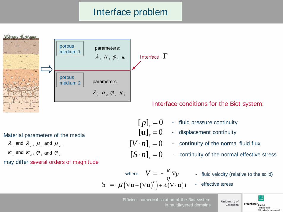
Interface conditions for the Biot system:

p Γ = [ ] 0 Γ =u [ ] 0 V n Γ

- fluid pressure continuity

- displacement continuity

⋅ = [ ] 0 S n Γ⋅ =

- continuity of the normal fluid flux

- continuity of the normal effective stress

- pV κη∇=

( )( ) ( ) T IS λμ ∇ + ∇ + ∇ ⋅= u u u

- fluid velocity (relative to the solid)

- effective stress

Interface problem

parameters:

parameters:

1λ 1μ 1ϕ1κ

2λ 2μ 2ϕ2κ

Interface

porousmedium 1

porousmedium 2

1

where

λ 2λMaterial parameters of the media

and

, 1

may differ several orders of magnitude

μ 2μand

,

1κ 2κ , 1ϕ 2ϕand and



and

Interface :

z ξ=

1κ

2κ

1λ 1μ

2λ 2μ ( ) 02

=⎥⎦

⎤⎢⎣

⎡∂∂

++⎟⎟⎠

⎞⎜⎜⎝

⎛∂∂

+∂∂

=ξ

μλλz

zw

yv

xu

0

=⎥⎦⎤

⎢⎣⎡

∂∂

=ξzzpk

0=⎥⎦

⎤⎢⎣

⎡⎟⎟⎠

⎞⎜⎜⎝

⎛∂∂

+∂∂

=ξ

μz

yw

zv

[ ] 0 ==ξzp

[ ] 0 ==ξzu

0=⎥⎦

⎤⎢⎣

⎡⎟⎠⎞

⎜⎝⎛

∂∂

+∂∂

=ξ

μzx

wzu

[ ] 0 ==ξzv [ ] 0 ==ξzwξ=z

elas

ticity

part

diff

usio

npa

rt2n

1n

3D model with horizontal plane interface



We use staggered grid to discretize the system *

u – component of the displacement

w – component of the displacementv – component of the displacement

Finite volume discretization. Staggered grid

- the domain is divided into 4 sets of control volumes

The finite volume discretization is derived:

- using the polinomials, which are piecewise – linear, extended with one special bilinear term in respectivedirection (for displacement components)

- using piecewise - trilinear polinomials (for fluid pressure)

- discretization near the interface resulted in some specificaveraging expressions for coefficients;

- numerical experiments showed that this discretizationprovides second order of convergence for basic variables as well as for fluxes of the problem in maximum norm.

pressure (in the vertices)

All these polinomials must satisfy interface continuityconditions

* following the work of P. Vabischevich, F. Lisbona, F. Gaspar „A FD analysis of Biot‘s consolidation model“

staggered grid in 3D



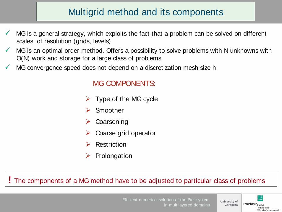
! The components of a MG method have to be adjusted to particular class of problems

MG COMPONENTS:

Type of the MG cycle

Smoother

Coarsening

Coarse grid operator

Restriction

Prolongation

MG is a general strategy, which exploits the fact that a problem can be solved on differentscales of resolution (grids, levels)MG is an optimal order method. Offers a possibility to solve problems with N unknowns with O(N) work and storage for a large class of problemsMG convergence speed does not depend on a discretization mesh size h

Multigrid method and its components



Convergence of a multigrid solver is strongly influenced by the jumps of the coefficients

For strongly jumping coefficients convergence may depend on the size of the jump and its location with respect to the grid lines. Even divergence may occur.

Smoother

Restriction

Coarse grid operator

Prolongation operator

IMPORTANT

- tri- (bi-) linear interpolation

- bicubic interpolation, etc.

- operator-dependent interpolation

- Accounts for the jumps of coefficients

- Rely on the interface continuityconditions (not continuity of the gradients)

Rely on the continuity of the errors and their gradients

PROLONGATION OPERATORS:

Multigrid for problems with strongly discontinuous coefficients



Operator-dependent prolongation

= p

p pp p

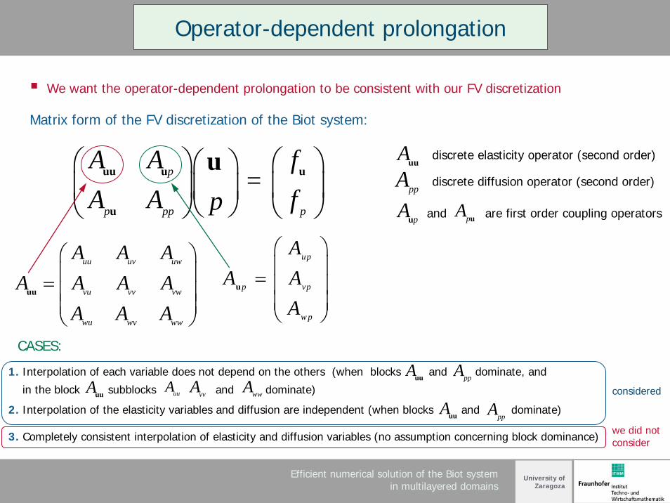
We want the operator-dependent prolongation to be consistent with our FV discretization

Matrix form of the FV discretization of the Biot system:

A A fA A fp

⎛ ⎞ ⎛ ⎞⎛ ⎞⎜ ⎟ ⎜ ⎟⎜ ⎟

⎝ ⎠⎝ ⎠ ⎝ ⎠

uu u u

u

u

uu uv uw

vu vv vw

wu wv ww

A A AA A A A

A A A

⎛ ⎞⎜ ⎟= ⎜ ⎟⎜ ⎟⎝ ⎠

uu

pA u

discrete elasticity operator (second order)Auu

ppApAu and are first order coupling operators

1. Interpolation of each variable does not depend on the others (when blocks and dominate, and

in the block subblocks and dominate)

2. Interpolation of the elasticity variables and diffusion are independent (when blocks and dominate)

3. Completely consistent interpolation of elasticity and diffusion variables (no assumption concerning block dominance)

up

p vp

wp

discrete diffusion operator (second order)

AA A

A

⎛ ⎞⎜ ⎟= ⎜ ⎟⎜ ⎟⎝ ⎠

u

Auu

Auu uuAwwA

ppAvvA

Auu ppA

we did notconsider

considered

CASES:



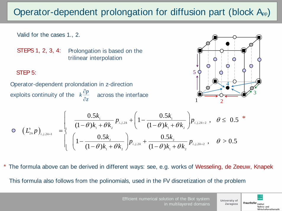
exploits continuity of the across the interfacepkz∂∂

Operator-dependent prolondation in z-direction

( )

1 1, ,2 , ,2 2

1 2 1 2

2 , ,2 1

2 2, ,2 , ,2 2

1 2 1 2

0.5 0.5 1 , 0.5(1 ) (1 )

0.5 0.5 1 , > 0.5

(1 ) (1 )

i j k i j k

hh i j k

i j k i j k

k kp pk k k k

L pk kp p

k k k k

θθ θ θ θ

θθ θ θ θ

+

+

+

⎧ ⎛ ⎞+ − ≤⎪ ⎜ ⎟− + − +⎪ ⎝ ⎠= ⎨

⎛ ⎞⎪ − +⎜ ⎟⎪ − + − +⎝ ⎠⎩

23

4

5

1

* The formula above can be derived in different ways: see, e.g. works of Wesseling, de Zeeuw, Knapek

This formula also follows from the polinomials, used in the FV discretization of the problem

STEP 5:

STEPS 1, 2, 3, 4: Prolongation is based on the trilinear interpolation

Operator-dependent prolongation for diffusion part (block App)

Valid for the cases 1., 2.

*



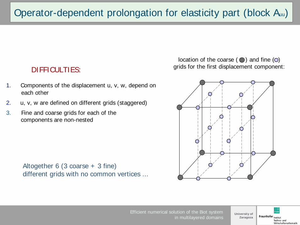
DIFFICULTIES:

1. Components of the displacement u, v, w, depend on each other

2. u, v, w are defined on different grids (staggered)

3. Fine and coarse grids for each of thecomponents are non-nested

location of the coarse ( ) and fine ( ) grids for the first displacement component:

Altogether 6 (3 coarse + 3 fine) different grids with no common vertices ...

Operator-dependent prolongation for elasticity part (block Auu)



Standard linear interpolation in x - and y - directionsOperator-dependent interpolation in z - direction

2 2 2 20.5 0.5 0.5

2 2( , , 0.25 ) 1 0.25 ( , ) 0.25 ( , )2 2k z k kw x y z h w x y w x yλ μ λ μ

λ μ λ μ− − +

⎛ ⎞+ ++ = − +⎜ ⎟⎜ ⎟+ +⎝ ⎠

1 1 1 10.5 0.5 0.5

2 2( , , 0.75 ) 0.25 ( , ) 1 0.25 ( , )2 2k z k kw x y z h w x y w x yλ μ λ μ

λ μ λ μ− − +

⎛ ⎞+ ++ = + −⎜ ⎟⎜ ⎟+ +⎝ ⎠

25.0<θ

21)1( θμμθμ +−=1 1 2 22 (0.5 )( 2 ) (0.5 )( 2 )λ μ θ λ μ θ λ μ+ = − + + + +where

e.g., interpolation in z direction of the w-component:

Rem: for u- and v- components the prolongation is done in a similar way

Operator-dependent prolongation for elasticity part. Case 1.

in the block subblocks and dominateAuu uuAwwAvvA

Interpolation of each displacement component does not depend on the others

Assumption:

For the considered interface problem we have to interpolate in the following way:



Standard linear interpolation in x - and y - directionsOperator-dependent interpolation in z - direction

( )( )

2 2 2 20.5 0.5 0.5

1 2, ,

2 2( , , 0.25 ) 1 0.25

0.5, ,

4 2 2

( , ) 0.25 ( , )2 2

2yxz

x k

k z k k

y k

hhh u x y v x

w x y z h w x y w y

y

xλ μ λ μλ μ λ μ

θ λ λλ μ

− − + +

⎛ ⎞− − ⎛ ⎞⎛ ⎞+ − + −⎜ ⎟⎜ ⎟⎜ ⎟

⎛ ⎞

+ ⎝ ⎠ ⎝

+ ++ = − +⎜ ⎟

⎠⎝

⎜ ⎟ +⎝ ⎠

⎠

+

( )( )

1 1 1 10.5 0.5 0.

1 2, ,

52 2( , , 0.75 ) 0.25 ( ,

0.5, ,

4

) 1 0.2

2 2 2

5 ( , )2 2k z

yxzy

k

x k k

k

h

w x y z h w x y

hh u

w x y

x y v x y

λ μ λ μλ μ λ μ

θ λ λλ μ

− − +

⎛ ⎞+ ++ = + −⎜ ⎟⎜ ⎟+ +⎝

−

⎛ ⎞+ − ⎛ ⎞⎛ ⎞− − + −⎜ ⎟⎜ ⎟⎜ ⎟+ ⎝ ⎠ ⎝ ⎠⎝ ⎠

⎠

e.g., interpolation in z direction of the w-component:

Rem: for u- and v- components the prolongation is done in a similar way

Operator-dependent prolongation for elasticity part. Case 2.

No assumption about the subblock dominance in Auu

For the considered interface problem we have to interpolate in the following way:

interpolation of displacement components depend on each other

Account for components u,vduring the interpolation of w-component

Account for components u,vduring the interpolation of w-component



Based on the standard prolongation

Cycle type: FNr of pre-smoothing steps: 3Nr of post-smoothing steps: 1Smoother: collective alternating lexicographic line GS

Domain: [0;1]x[0;1]x[0;1]Time: [0;10^-1]

0.501ξ =

1 21, 10λ λ= = 1 21, 10μ μ= = 1 21, 10k k= =

Based on the operator-dependent prolongation

Numerical experiment 1. MG* convergence.

* the MG code is an extension (for the case of discontinuous coefficients) of the MG poroelasticity code, written byC.W. Oosterlee and F. Gaspar

Coefficients:(jumps one order

of magnitude)



Based on the standard prolongation Based on the operator-dependent prolongation *

Numerical experiment 2. MG convergence.

Cycle type: FNr of pre-smoothing steps: 3Nr of post-smoothing steps: 1Smoother: collective alternating lexicographic line GS

Domain: [0;1]x[0;1]x[0;1]Time: [0;10^-1]

0.501ξ =

7 1 21, 10λ λ= =

7 1 21, 10μ μ= =

7 1 21, 10k k= =

Coefficients:(jumps 7 orders

of magnitude)

* the prolongations 1 and 2 for this test example give identical results



Summary

Biot model with discontinuous coefficients was considered

Finite volume discretization, which provides second order of convergence for the primary as well as flux variables was derived

Operator-dependent prolongation was derived in order to provideMG covergence in the case of discontinuous coefficients

A set of numerical experiments was carried out



Date post:	07-Feb-2018
Category:	Documents
Upload:	doanhuong
View:	230 times
Download:	0 times

Efficient numerical solution of the Biot poroelasticity ... · PDF fileEfficient numerical...

Documents