Efficient regular expressions that produce parse treesscg.unibe.ch/archive/masters/Karp14a.pdf · 8...

UNIVERSITY OF BERN

Efficient regular expressions that produceparse trees

by

Aaron Karper

A thesis submitted in partial fulfillment for thedegree of Master of Science

in thePhilosophisch-naturwissenschaftliche Fakultät

Institute of Computer Science and Applied Mathematics

supervised by

Prof. Oscar Nierstrasz and Dr. Niko Schwarz

December 19, 2014

http://www.unibe.ch

http://www.philnat.unibe.ch/

http://www.iam.unibe.ch/en

UNIVERSITY OF BERN

AbstractPhilosophisch-naturwissenschaftliche Fakultät

Institute of Computer Science and Applied Mathematics

Master of Science

by Aaron Karper

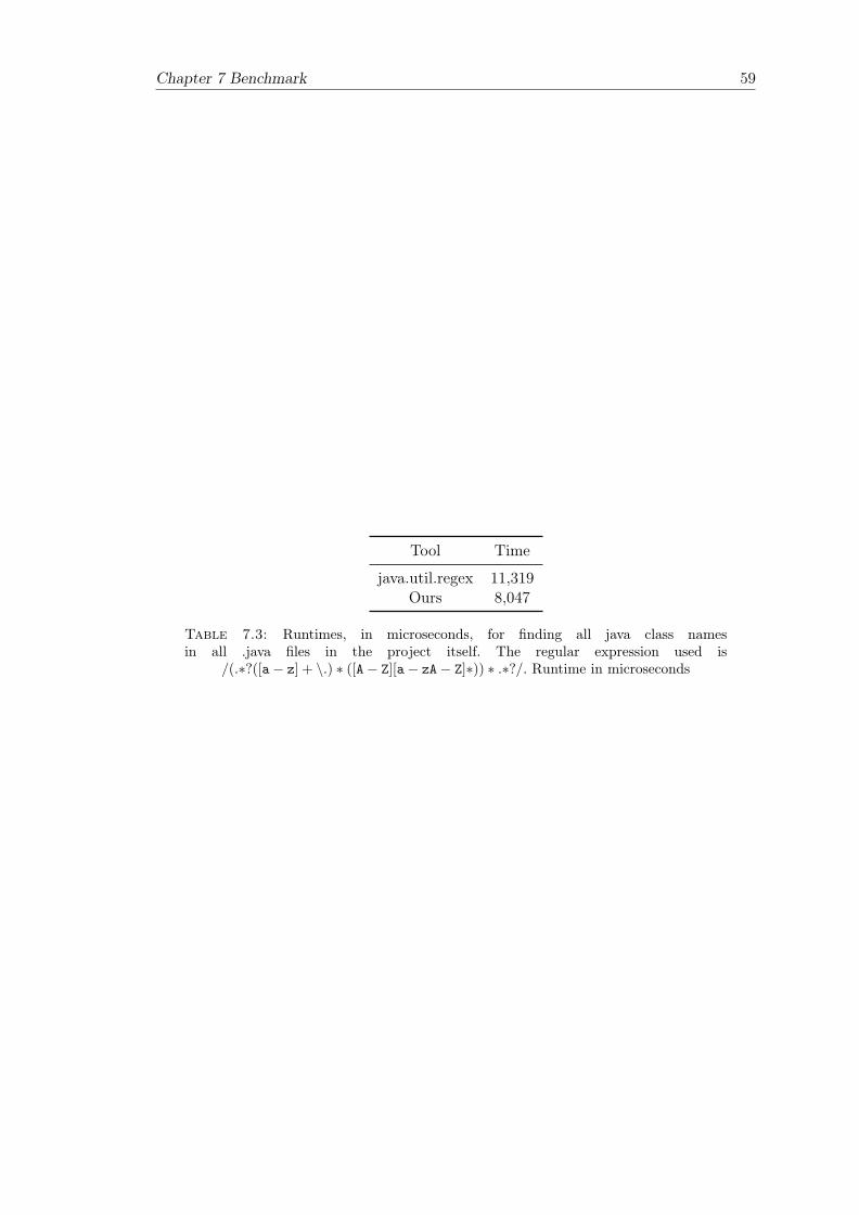
Regular expressions naturally and intuitively define parse trees that describe the textthat they’re parsing. We describe a technique for building up the complete parse treeresulting from matching a text against a regular expression.

In previous tagged deterministic finite-state automaton (TDFA) matching implementa-tions, all paths through the non-deterministic finite-state automaton (NFA) are walkedsimultaneously, in different co-routines, where inside each co-routine, it is fully knownwhen which capture group was entered or left. We extend this model to keep track of notjust the last opening and closing of capture groups, but all of them. We do this by storingin every co-routine a history of the all groups using the flyweight pattern. Thus, we logenough information during parsing to build up the complete parse tree after matching ina single pass, making it possible to use our algorithm with strings exceeding the machine’smemory. Further we construct the automata such that a simulation of backtracking likebehaviour is possible. This is achieved in worst case time Θ(mn), providing full parsetrees with only constant slowdown compared to matching.

http://www.unibe.ch

http://www.philnat.unibe.ch/

http://www.iam.unibe.ch/en

Contents

Contents 5

1 Introduction 71.1 More powerful than standard regular expressions . . . . . . . . . . . . . . 81.2 Motivation . . . . . . . . . . . . . . . . . . . . . . . . . . . . . . . . . . . . 81.3 Regular expressions . . . . . . . . . . . . . . . . . . . . . . . . . . . . . . . 9

Literals . . . . . . . . . . . . . . . . . . . . . . . . . . . . . 10Character ranges . . . . . . . . . . . . . . . . . . . . . . . . 10Negated character ranges . . . . . . . . . . . . . . . . . . . . 10Concatenation . . . . . . . . . . . . . . . . . . . . . . . . . . 10Option operator . . . . . . . . . . . . . . . . . . . . . . . . . 10Star operator . . . . . . . . . . . . . . . . . . . . . . . . . . 10Plus operator . . . . . . . . . . . . . . . . . . . . . . . . . . 10Non-greedy operators . . . . . . . . . . . . . . . . . . . . . . 10Alternation . . . . . . . . . . . . . . . . . . . . . . . . . . . 10

1.3.1 Capture groups . . . . . . . . . . . . . . . . . . . . . . . . . . . . . 11Greediness . . . . . . . . . . . . . . . . . . . . . . . . . . . . 11

1.4 Backtracking . . . . . . . . . . . . . . . . . . . . . . . . . . . . . . . . . . 111.5 (Non-)deterministic finite-state automata . . . . . . . . . . . . . . . . . . 12

2 Algorithm 152.1 NFA based matching . . . . . . . . . . . . . . . . . . . . . . . . . . . . . . 152.2 DFA based matching . . . . . . . . . . . . . . . . . . . . . . . . . . . . . . 152.3 Lazy DFA compilation . . . . . . . . . . . . . . . . . . . . . . . . . . . . . 162.4 Tagged finite state automata . . . . . . . . . . . . . . . . . . . . . . . . . 17

2.4.1 Simulating backtracking for regular expressions . . . . . . . . . . . 182.5 Pipeline . . . . . . . . . . . . . . . . . . . . . . . . . . . . . . . . . . . . . 182.6 Thompson’s construction . . . . . . . . . . . . . . . . . . . . . . . . . . . . 192.7 Logging capture groups in a TNFA . . . . . . . . . . . . . . . . . . . . . . 21

2.7.1 Conversion to tagged DFA . . . . . . . . . . . . . . . . . . . . . . . 27

3 Data structures 293.1 Fully persistent data structures . . . . . . . . . . . . . . . . . . . . . . . . 293.2 Copy-on-write array . . . . . . . . . . . . . . . . . . . . . . . . . . . . . . 303.3 Treap . . . . . . . . . . . . . . . . . . . . . . . . . . . . . . . . . . . . . . 313.4 Storing updates . . . . . . . . . . . . . . . . . . . . . . . . . . . . . . . . . 31

3.4.1 Linear versions . . . . . . . . . . . . . . . . . . . . . . . . . . . . . 32

5

6 CONTENTS

3.4.2 Version tree . . . . . . . . . . . . . . . . . . . . . . . . . . . . . . . 32Emptying a full buffer . . . . . . . . . . . . . . . . . . . . . 33Constant time ordering of versions . . . . . . . . . . . . . . 33

3.5 Order maintenance . . . . . . . . . . . . . . . . . . . . . . . . . . . . . . . 353.5.1 Relabeling . . . . . . . . . . . . . . . . . . . . . . . . . . . . . . . . 353.5.2 Indirection . . . . . . . . . . . . . . . . . . . . . . . . . . . . . . . 36

4 Proofs 394.1 Correctness . . . . . . . . . . . . . . . . . . . . . . . . . . . . . . . . . . . 394.2 Execution time . . . . . . . . . . . . . . . . . . . . . . . . . . . . . . . . . 424.3 Lower bound for time . . . . . . . . . . . . . . . . . . . . . . . . . . . . . 43

5 Implementation 455.1 DFA transition table . . . . . . . . . . . . . . . . . . . . . . . . . . . . . . 455.2 DFA execution . . . . . . . . . . . . . . . . . . . . . . . . . . . . . . . . . 465.3 Compactification . . . . . . . . . . . . . . . . . . . . . . . . . . . . . . . . 465.4 Intertwining of the pipeline stages . . . . . . . . . . . . . . . . . . . . . . . 485.5 Parsing the regular expression syntax . . . . . . . . . . . . . . . . . . . . . 48

6 Related work 516.1 Revisiting backtracking . . . . . . . . . . . . . . . . . . . . . . . . . . . . 526.2 Packrat parsers . . . . . . . . . . . . . . . . . . . . . . . . . . . . . . . . . 536.3 Automata based extraction of parse trees . . . . . . . . . . . . . . . . . . 546.4 Large scale data analysis of a stream of text . . . . . . . . . . . . . . . . . 55

7 Benchmark 57

8 Conclusion 61

Appendices 63

A Minimal python implementation 65A.1 Construction . . . . . . . . . . . . . . . . . . . . . . . . . . . . . . . . . . 65A.2 Matching . . . . . . . . . . . . . . . . . . . . . . . . . . . . . . . . . . . . 67

Bibliography 71

List of Figures 71

List of Tables 75

List of Algorithms 77

Chapter 1

Introduction

Regular expressions give us a concise language to describe patterns in strings and canbe used for log analysis, natural language processing, and many other tasks involvingstructured data in strings. Their efficiency make them useful even for large data sets.Standard algorithms run in O(nm), where n is the length of the string to be matchedagainst and m is the length of the pattern [25].

A short-coming of standard regular expression engines is that they can extract only alimited amount of information from the string. A regular expression can easily describethat a text matches a comma separated values file, but it is unable to extract all thevalues. Instead it only gives a single instance of values:

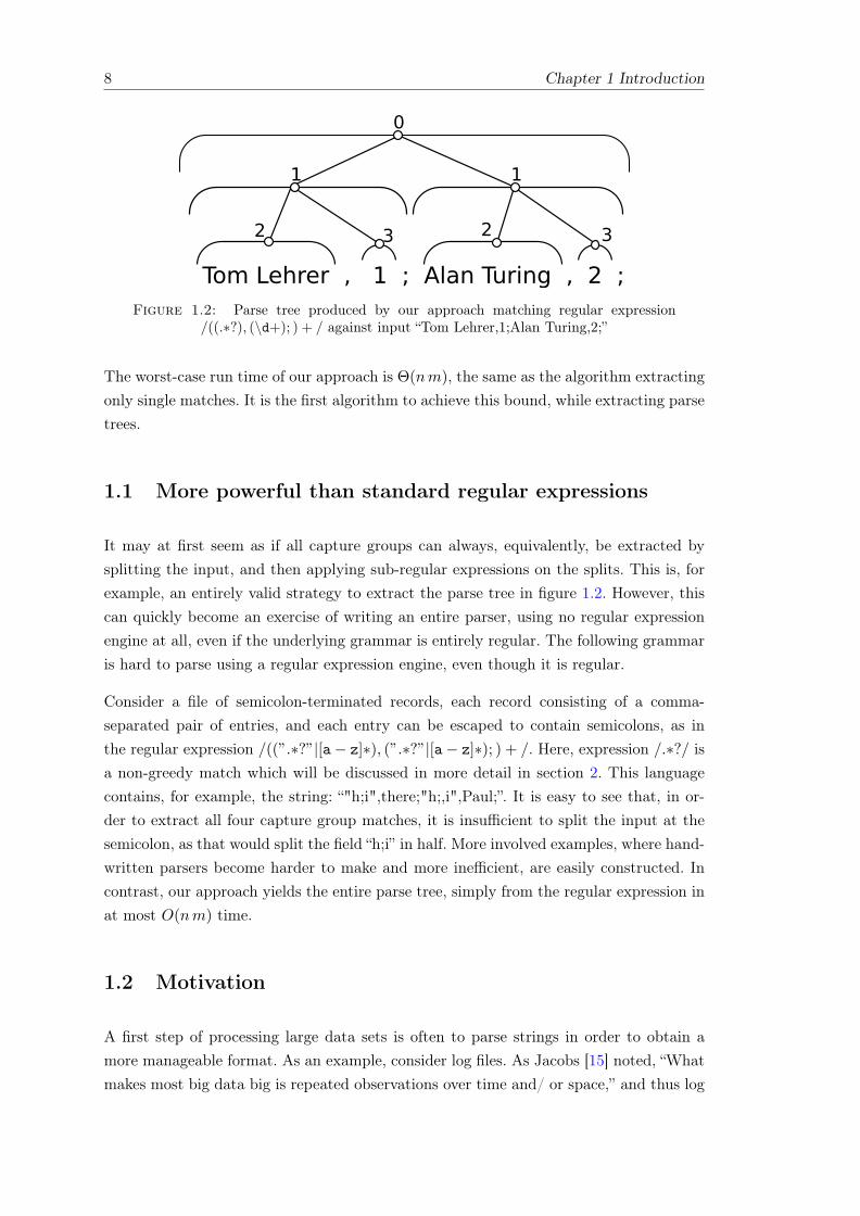
/((.∗?), (\d+); ) + / might describe a dataset of ASCII names with their numeric label.Matching the regular expression on “Tom Lehrer,1;Alan Turing,2;” confirms that thelist is well formed, but the match contains only “Tom Lehrer” for the second capturegroup and “1” for the third. That is, the parse tree found by the Posix is seen infigure 1.1.

Tom Lehrer , 1 ; Alan Turing , 2 ;

2 3

0

1

Figure 1.1: Parse tree produced by Posix-compatible matching /((.∗?), (\d+); ) + /against input “Tom Lehrer,1;Alan Turing,2;”.

With our algorithm we are able to reconstruct the full parse tree after the matchingphase is done, as seen in figure 1.2.

7

8 Chapter 1 Introduction

Tom Lehrer , 1 ; Alan Turing , 2 ;

2 3

0

1 1

32

Figure 1.2: Parse tree produced by our approach matching regular expression/((.∗?), (\d+); ) + / against input “Tom Lehrer,1;Alan Turing,2;”

The worst-case run time of our approach is Θ(nm), the same as the algorithm extractingonly single matches. It is the first algorithm to achieve this bound, while extracting parsetrees.

1.1 More powerful than standard regular expressions

It may at first seem as if all capture groups can always, equivalently, be extracted bysplitting the input, and then applying sub-regular expressions on the splits. This is, forexample, an entirely valid strategy to extract the parse tree in figure 1.2. However, thiscan quickly become an exercise of writing an entire parser, using no regular expressionengine at all, even if the underlying grammar is entirely regular. The following grammaris hard to parse using a regular expression engine, even though it is regular.

Consider a file of semicolon-terminated records, each record consisting of a comma-separated pair of entries, and each entry can be escaped to contain semicolons, as inthe regular expression /((”.∗?”|[a− z]∗), (”.∗?”|[a− z]∗); ) + /. Here, expression /.∗?/ isa non-greedy match which will be discussed in more detail in section 2. This languagecontains, for example, the string: “"h;i",there;"h;,i",Paul;”. It is easy to see that, in or-der to extract all four capture group matches, it is insufficient to split the input at thesemicolon, as that would split the field “h;i” in half. More involved examples, where hand-written parsers become harder to make and more inefficient, are easily constructed. Incontrast, our approach yields the entire parse tree, simply from the regular expression inat most O(nm) time.

1.2 Motivation

A first step of processing large data sets is often to parse strings in order to obtain amore manageable format. As an example, consider log files. As Jacobs [15] noted, “Whatmakes most big data big is repeated observations over time and/ or space,” and thus log

Chapter 1 Introduction 9

files grow large frequently. At the same time, they provide important insight into theprocess that they are logging, so their parsing and understanding is important.

Regular expressions make for scalable and efficient lightweight parsers [16].

The parsing abilities of regular expression have provoked Meiners to declare that forintrusion detection, “fast and scalable RE matching is now a core network security issue.”[21]

For example, Arasu et al. [1] demonstrate how regular expressions are used in Bing tovalidate data, by checking whether the names of digital cameras in their database arevalid.

Parsers that can return abstract syntax trees are more useful than ones that only give aflat list of matches. Of course only regular grammars can be matched by our approach.

1.3 Regular expressions

Before we dive into the algorithm to match regular expressions, we should first look atthe goal – what regular expressions are and what kind of constructs need to be supportedby our algorithm.

Regular expressions have some constructs specific to them and literal character matches.They are typically described in a string describing the pattern. They can describe anyregular language [26] if one only considers match vs non-match though they are typicallyused to extract information.

Name Example Repetitions Descriptionliteral /a/ 1

character ranges /[a− z]/ 1 any of the characters in therange match

negated character ranges /[ˆa− z]/ 1 anything except for thecharacters in the range match

? operator /a?/ 0 or 1* operator /a ∗ / 0−∞ Prefer more matched+ operator /a + / 1−∞?? operator /a??/ 0 or 1*? operator /a∗?/ 0−∞ Prefer less matched+? operator /a+?/ 1−∞

alternation operator /a|b/ 1 match one or the other,prefer left

capture groups /(a)/ 1 treat pattern as singleelement, extract match

Table 1.1: Summary of regular expression elements


Literals The simplest form of regular expressions are literal characters like /a/.

Character ranges Instead of matching only a single character, a regular expressionmight match any of a range of characters. This is denoted with brackets. For example/[a− z]/ would match any lowercase ASCII letter, /[abc]/ would only match the lettersa, b, or c, and /[a− gk− t]/ would match any letter between a and g, or between k andt. There is also the special character range /./ that matches any character.

Negated character ranges Ranges of the form /[ˆ . . . ]/ negate their content, so/[ˆa− g]/ would match anything except a through g.

Concatenation Two constructs put after each other have to match the string in order.For example /a[bc]/ matches “a” followed by either “b” or “c”.

Option operator The option operator denoted by /?/ allows either zero or onerepetitions of the preceding element, preferring to have one repetition. This means /a?/

will match the empty string or “a”, but nothing else.

Star operator The star operator * allows for arbitrary repetition of the preceding el-ement, including zero repetitions, preferring as many repetitions as possible. For example/a ∗ / matches the empty string, “a”, “aa”, and so on.

Plus operator The plus operator + is similar, but requires at least one repetition.This leads to /a + / and /aa ∗ / matching the same strings.

Non-greedy operators The option, the star, and the plus operators also have cor-responding non-greedy operators, which are ??, /∗?/, and /+?/ respectively. These op-erators prefer to match as few repetitions as possible. In back-tracking implementation,guessing the right path is an important efficiency feature and for all capturing imple-mentation the path taken influences the captured groups.

Alternation Patterns separated by the pipe symbol | can either match the left partor the right part. This binds weaker than concatenation. Therefore /abc|xyz/ wouldmatch “abc” or “xyz”, but not “abxyz”.


1.3.1 Capture groups

Patterns enclosed by parentheses are treated as a single element, thus /(ab) ∗ / cap-tures “ab”, but not “aba”. More importantly for us is that after the match, the capturegroups can be extracted: /a(b∗)c/ when matching “abbbc” can extract “bbb” and theempty string when matching “ac”. Note that the capture groups can be nested and thesemantics differ for Posix and tree regular expressions: In Posix the regular expression/a((bc+)+)/ on the string “abcbccc” gives “bcbccc” for the outer capture group and bcfor the inner capture group – the leftmost occurrence of outer capture groups is kept andwithin that substring, the leftmost occurrence of the inner group is kept. In tree regularexpressions, all occurrences are kept and returned in a tree structure: The outer capturegroup contains “bcbccc” and both inner matches “bc” and “bccc”.

Greediness The relevance of greedy and non-greedy matches becomes apparent now:The regular expression /a(.∗)c?/ on the string “abc” captures “bc” in the group, while/a(.∗?)c?/ captures only “b”. This is because the parsing is ambiguous without specifyingthe greediness of the match – both “b” and “bc” would be valid.

1.4 Backtracking

An intuitive and extensible algorithm for determining whether a string matches a regularexpression is backtracking. This algorithm 1 is used as is or in a more optimized form inmany languages, such as Java1, Python2, or Perl [5]. For all its advantages and ease ofimplementation the main problem is that it takes Θ(2nm) time in the worst case:

If we have the pattern /(x∗) ∗ y/ matching against the string3 xn, we see that it cannotmatch, but it takes exponential time doing so. In each step there are two options, eitherto collect the x in /x ∗ /, or to step over it and try again. Unfortunately that means thatthe algorithm branches in each character in the string and never succeeding keeps ontrying, so it takes 2n steps to end in the no match case. Backtracking is fast if it guessescorrectly, since there is not much overhead, but fails miserably if it guesses wrongly earlyon.

Because backtracking is so intuitive we will use it as the definition of a correct behaviourthroughout this thesis.

1java.util.regex2The module re3xn means x repeated n times


Algorithm 1 Overview of backtrackingfunction match-bt(string, pattern)

if string and pattern empty thenreturn matches

else if string or pattern empty thenreturn no match

else if first element of pattern is a∗ then. x[1:] means removing the first element of the listif a matches first element of string then

return match-bt(string[1:], pattern)else

return match-bt(string, pattern[1:])end if

else if . . . then. . .

end ifend function

1.5 (Non-)deterministic finite-state automata

As they are heavily used throughout this paper, let us recall what non-deterministic finite-state automata (NFA) and deterministic finite-state automata (DFA) are. A DFA is astate machine that walks over a finite transition graph, one step for every input character.The choice of transition is limited by the transition’s character range. A transition canonly be followed if the current input character is inside transition’s character range. Thepossible character ranges are assumed to be disjoint, so that in every step at most onetransition can be followed.

NFA differ from DFA in that for some input character and some state, there may be morethan one applicable transition and some transitions can be traversed without consuminga character, called ε-transitions. If there is a transition that leads to the accepting stateeventually, an NFA finds it, by trying the alternatives in lock-step. Figure 2.2 shows anexample of an NFA’s transition graph.

An simple way to think about the process of reading input with an NFA is that ofco-routines. Co-routines are procedures that has the ability to suspend themselves andcontinue later – they are similar to threads, but co-routines don’t need to be executedin parallel and are usually manually scheduled. In order to resume their work later, theycontain some kind of memory that is specific to them.

In the context of NFAs, a co-routine contains the current state and has access to thetransition graph4. When reading a string, the NFA maintains a set of co-routines andrun them in lock-step. This means that each co-routine reads the current characterand spawns new co-routines for all possible transitions. When reading a character, a

4Later more memory will be added to store the sub-matches.


co-routine must consume it, but might follow ε-transitions before. We model this byfollowing ε-transitions in order, and whenever we encounter a transition that can consumethe current character, the state following it is added to the next scheduling cycle.

Furthermore the order in which states are expanded will become relevant: a transitionthat crossed a tag and one that doesn’t cross a tag can end in the same state – dependingon the order the memory of the coroutine in the state differs. Since we still store at mostone co-routine in any NFA-state, the co-routines compete to capture a state. The winner– that is the first co-routine to enter a state – will define the memory of all followingstates. For this, the model of the NFA is expanded for allowing transitions with negativepriority. An edge with negative priority will only be expanded when there are no morelegal transitions with regular priority. The order for high and low priorities is depth first5.

5In an implementation this would imply that a newly seen state is put on a stack.

Chapter 2

Algorithm

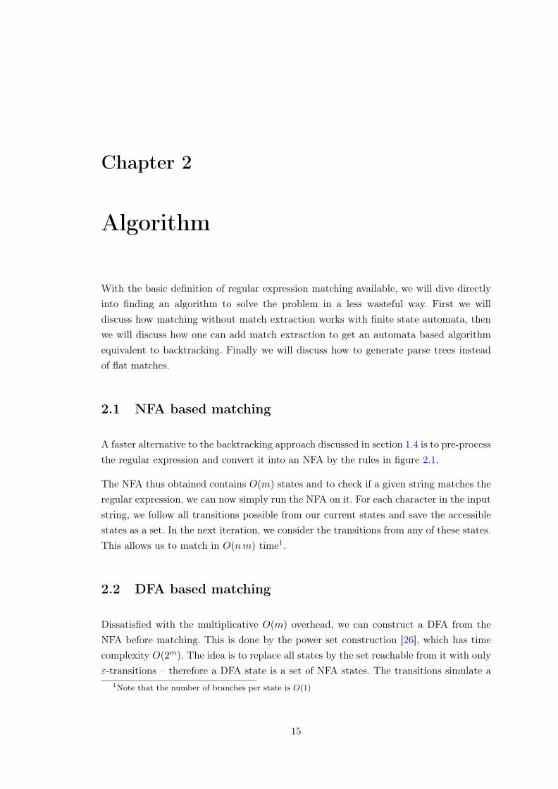
With the basic definition of regular expression matching available, we will dive directlyinto finding an algorithm to solve the problem in a less wasteful way. First we willdiscuss how matching without match extraction works with finite state automata, thenwe will discuss how one can add match extraction to get an automata based algorithmequivalent to backtracking. Finally we will discuss how to generate parse trees insteadof flat matches.

2.1 NFA based matching

A faster alternative to the backtracking approach discussed in section 1.4 is to pre-processthe regular expression and convert it into an NFA by the rules in figure 2.1.

The NFA thus obtained contains O(m) states and to check if a given string matches theregular expression, we can now simply run the NFA on it. For each character in the inputstring, we follow all transitions possible from our current states and save the accessiblestates as a set. In the next iteration, we consider the transitions from any of these states.This allows us to match in O(nm) time1.

2.2 DFA based matching

Dissatisfied with the multiplicative O(m) overhead, we can construct a DFA from theNFA before matching. This is done by the power set construction [26], which has timecomplexity O(2m). The idea is to replace all states by the set reachable from it with onlyε-transitions – therefore a DFA state is a set of NFA states. The transitions simulate a

1Note that the number of branches per state is O(1)

15

16 Chapter 2 Algorithm

S2

S1

Alternation

S1|S2

S

Plus operation

S+

S

Optional

S?

S

Star operation

S*?

Figure 2.1: Thompson [28] construction of the automaton: Descend into the abstractsyntax tree of the regular expression and expand the constructs recursively.

step in the original NFA, so they point to another set of states. After the compilation isdone, matching the string is O(n) time.

This can be very useful, if the regular expression is statically known.

2.3 Lazy DFA compilation

The DFA based matching takes O(n+ 2m), which is no better than backtracking if m isnot fixed. The power set construction simulates every transition possible in the NFA, butthat is actually unnecessary: Instead we can intertwine the compilation and the matchingto only expand new DFA states that are reached when parsing the string. At most onenew DFA state is created after each character read and if necessary the whole DFA isconstructed, after which the algorithm is no different from the eager DFA. The timecomplexity of the match is then O(min(nm,n+ 2m)).

This is the best known result for matching [5, 6, 7].

Note however that for many matches, nm is at least as good as n + 2m, and in thosecases, this gives no improvement over the NFA matching.

Our algorithm modifies this algorithm by adding instructions to transitions, but the corepart is the modification of the NFA construction.

Chapter 2 Algorithm 17

2.4 Tagged finite state automata

The algorithms so far did not extract capture groups, because they have no informationabout where a capture group starts or ends. In order to extract this information, we needto store it in some way, as we traverse the automaton.

Remember that NFA interpretation can be thought as competing co-routines, runningin lock-step with each step consuming exactly one character of the input string2 Thismodel already implies that some form of instructions are executed on a transition, so itis possible to add other instructions that allow us to store the capture groups. This isthe idea of the tagged finite state automaton3, which attaches general tags to transitionsthat modify the co-routine’s memory in some way. This way, co-routines can store thecomplete information, where they matched which capture group in their own memory.

Specifically we can store the position of the start and end of each match in the memoryof the co-routine, whenever we encounter a transition that corresponds to the start orend of a capture group.

Side effects, such as storing the current location, make co-routines using different routesto the same state differ in meaning. Consider the regular expression /(a)|(.)/ reading thestring “a”: depending on the path chosen our capture groups will either contain “a” inthe first or second capture group. This requires us to define a unique order for expandingco-routines on each state, so that we can avoid this ambiguity. This is avoided by givinga negative priority4 to one of the transitions or require one to consume a character,whenever we have an out-degree of two5.

The priorities intuitively mean that for example in /.a|../ we will try to follow the pathof /.a/ first before checking /../. Only if we fail on that track we will consider the secondpath.

Closely related to priorities is greediness control: Consider again the regular expression/((.∗?), (\d+); ) + /. The question mark sets the /. ∗ / part of the regular expressionto non-greedy, which means that it matches as little as possible while still producing avalid match, if any. Without provisioning /. ∗ / to be non-greedy, a matching againstinput “TomLehrer, 1; AlanTuring, 2;” would match as much as possible into the firstcapture group, including the record separator “,”. Thus, the first capture group wouldsuddenly contain only one entry, and it would contain more than just names, namely“TomLehrer, 1; AlanTuring”. This is, of course, not what we expect. Non-greediness,here, ensures that we get “TomLehrer”, then “AlanTuring” as the matches of the firstcapture group.

2The empty string can be modelled as containing only the ‘\0’ character.3First called that by Laurikari [19]4See also Laurikari [19]5Note that in the Thompson construction, we have an out-degree of at most two.


Implementing this in a backtracking implementation is trivial, but in order to keep theco-routines in lock-step, we need to order the NFA states in the DFA state, so that theco-routines travelling the left path are always scheduled before the routines on the rightpath.

To complicate things further, we want co-routines that travelled further to have higherpriority than the ones that stayed further behind – in backtracking this would be depth-first-search.

Section 2.4.1 will explain how this can be simulated in TNFA interpretation, which is anoriginal contribution of this paper.

2.4.1 Simulating backtracking for regular expressions

In order to simulate backtracking correctly, we need that all paths reachable from thestate after the prioritized transition is processed first, even if interrupted by the need toconsume another character. This prioritization is achieved by using a buffer, that reversesthe order of high-priority runs.

Without the buffer, the routines are scheduled in the order in which the states are seen.This gives wrong results, if the state further behind can catch up to one further down,for example in /(a∗?)(a∗?)/, the second group should contain the match.

2.5 Pipeline

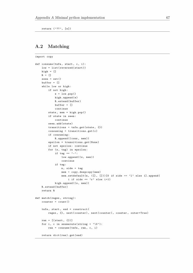
The algorithm we present is specific case of the tagged non-deterministic finite stateautomaton (TNFA) matching algorithm for regular expressions with added logging ofthe start and end of capture groups, as described in section 2.4. We first present thealgorithm for matching, which is O(nmu(m)), where u(m) describes the amortized costof logging a single opening or closing of a capture group. We then show a simple datastructure that allows us to achieve u(m) = logm and continue to present a way toimprove this to u(m) = 1 following Driscoll et al [9]. This gives us O(nm) run time forthe complete algorithm, which is the best known run time for NFA algorithms. We alsoconsider practical problems such as caching current results, just-in-time compilation, andcompact memory usage.

Conceptually, our approach consists of four stages:

1. Parse the regular expression string into an AST (section 5.5).

2. Transform the AST to an NFA (section 2.6).

3. Transform the NFA to a DFA (section 2.7).


Algorithm 2 Tagged transition execution. See appendix A.2 for an actual implementa-tion in Python.. Returns a list of co-routines that consumed the characterfunction runtagged(coroutines, char)

. coroutines is a list of co-routines in order as returned here.

. char is a characterPut all coroutines on the low stackInitialize empty buffer stackInitialize empty list R . the returned list of co-routineswhile the stacks aren’t both empty do

if high is not empty thenPop c from the high stack

elsePop c from the low stackFlush buffer into R, thus reversing the order

end iffor all transitions that consume char from c to state s do

. We remember the state for the next turnpush s to buffer

end forfor all ε-transitions from c to state s with tag t do

if no co-routine in state s exists in coroutines thencopy the co-routine c to c′

interpret(t, c′)end ifif transition is normal priority then

add a co-routine r in state s with memory m to the high stackelse

add a co-routine r in state s with memory m to the low stackend if

end forend whilereturn R

end function

4. Compactify the DFA (section 5.3).

In reality, things are a little more involved, since the transformation to DFA is lazy, andthe compactification only happens after no lazy compilation has occurred in a while. Alsocompactification can be undone if needed. Since the essence of the algorithm is step 2and 3, we start with them and proceed to see steps 1 and 4 as part of the implementation.

2.6 Thompson’s construction

We transform the abstract syntax tree (AST) of the regular expression into a TNFA,in a modified version of Thompson’s NFA construction. Tagged transitions mark the


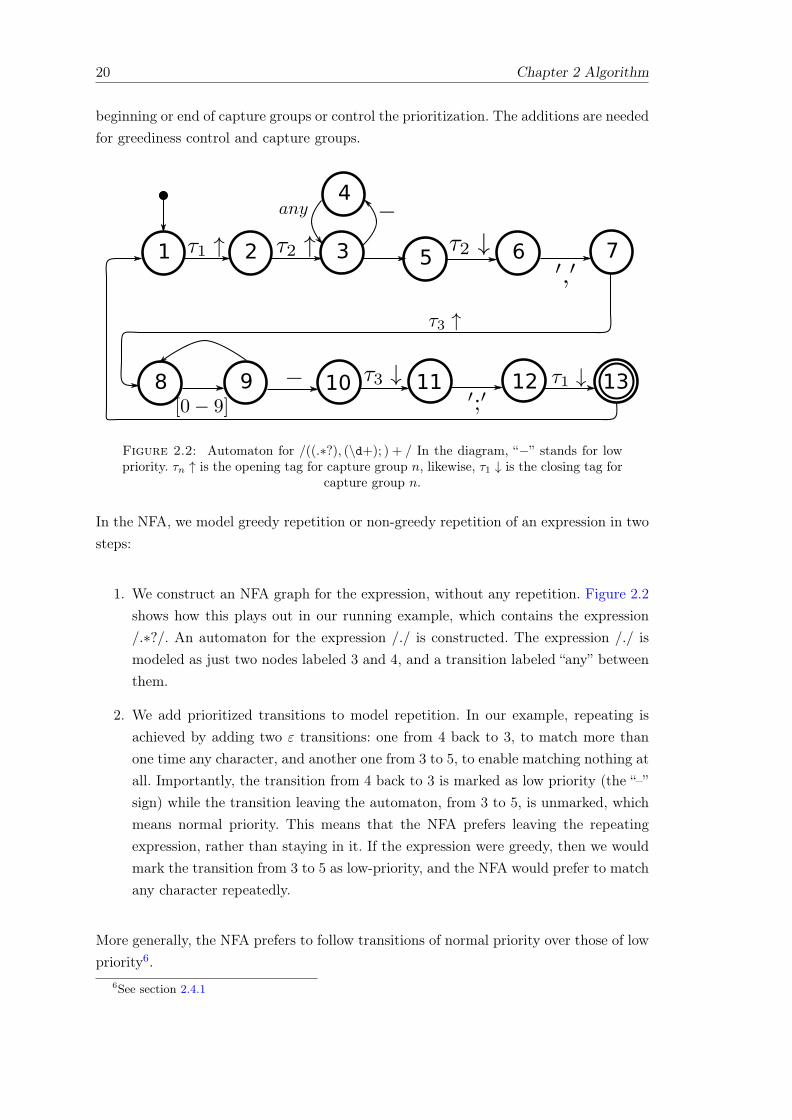
beginning or end of capture groups or control the prioritization. The additions are neededfor greediness control and capture groups.

1 2 3

4

6 7

8 9 11 12 1310

5

Figure 2.2: Automaton for /((.∗?), (\d+); ) + / In the diagram, “−” stands for lowpriority. τn ↑ is the opening tag for capture group n, likewise, τ1 ↓ is the closing tag for

capture group n.

In the NFA, we model greedy repetition or non-greedy repetition of an expression in twosteps:

1. We construct an NFA graph for the expression, without any repetition. Figure 2.2shows how this plays out in our running example, which contains the expression/.∗?/. An automaton for the expression /./ is constructed. The expression /./ ismodeled as just two nodes labeled 3 and 4, and a transition labeled “any” betweenthem.

2. We add prioritized transitions to model repetition. In our example, repeating isachieved by adding two ε transitions: one from 4 back to 3, to match more thanone time any character, and another one from 3 to 5, to enable matching nothing atall. Importantly, the transition from 4 back to 3 is marked as low priority (the “–”sign) while the transition leaving the automaton, from 3 to 5, is unmarked, whichmeans normal priority. This means that the NFA prefers leaving the repeatingexpression, rather than staying in it. If the expression were greedy, then we wouldmark the transition from 3 to 5 as low-priority, and the NFA would prefer to matchany character repeatedly.

More generally, the NFA prefers to follow transitions of normal priority over those of lowpriority6.

6See section 2.4.1


S2

S1

-

AlternationS1|S2

S -

Plus operationS+

S

-

OptionalS?

S

Capture group(S)

S

-Non-greedy plus operation

S+?

S

-

Non-greedy star operationS*?

S

-

Star operationS*?

-

Figure 2.3: Modified Thompson [28] construction of the automaton: Descend into theabstract syntax tree of the regular expression and expand the constructs recursively. Incomparison to the simple construction in figure 2.1, the forward transitions from thetop state in the star operators should be surprising, but they are necessary if S has aprioritized path that captures the empty string: We cannot return to the start state,

because we expanded it already, but we can proceed anyway.

2.7 Logging capture groups in a TNFA

Our algorithm is directly based on algorithm 2, so this section lays out the storagerequired by the co-routines and the interpretation of the tags that we introduced in theprevious section.

To model capture groups in the NFA, we add commit tags to the transition graph. Thetransition into a capture group is tagged by a commit, the transition to leave a capturegroup is tagged by another commit. We distinguish opening and closing commits. TheNFA keeps track of all times that a transition with an attached commit was used, thuskeeping the history of each commit. After parsing succeeds, the list of all histories canthen be used to reconstruct all matches of all capture groups.

We model histories as singly linked lists, where the payload of each node is a position.Only the payload of the head, the first node, is mutable, the rest, all other nodes, are


25

9

6 7

24

Figure 2.4: Histories are cells of singly linked lists, where only the first (here bottom-most) cell can be edited. This is a view of the automaton in figure 2.2 after the string“TomLehrer, 1; AlanTuring,” has been consumed. Only the cell for the closing of the

second capture group is shown.

immutable. Because the rests are immutable, they may be shared between histories.This is an application of the flyweight pattern, which ensures that all of the followinginstructions on histories can be performed in constant time. Here, the position is thecurrent position of the matcher.

Notation. We use the following vocabulary.

DFA states are denoted by a capital letter, e.g. Q, and contain multiple co-routines.

Q = [(q1, (([0], [12]), ([9, 1], [10, 2]), ([], []))),

(q2, (([0], []), ([1], [2]), ([1], [2])))]

for example means that the current DFA state has one co-routine in NFA stateq1 with histories (([0], [12]), ([9, 1], [10, 2])) and another co-routine in NFA stateq2 with the histories (([0], []), ([1], [2]), ([1], [2])). Note that histories can be sharedacross co-routines if they have the same matches. The order of the co-routines isrelevant and a DFA state is thus a list of NFA states.

Histories are linked lists, where each node stores a position in the input text. Thehead is mutable, and the rest is immutable. Therefore, histories can share anynode except their heads. We write h = [x1, . . . , xm] to describe that matches haveoccurred at the positions x1, . . . , xm.

Co-routines are denoted as pairs (qi, h), where qi is some NFA state, and h = (h1, . . . , h2n)

is an array of histories, where n is the number of capture groups. Each co-routinehas an array of 2n histories. In an array of histories ((h1, h2), . . . (h2n−1, h2n)), his-tory h1 is the history of the openings of the first capture group, and h2 is the


history of the closings of the first capture group, and so on. The visual pairing ofthe histories is in order to visualize which histories denote start and end of whichcapture group.

Transitions are understood to be between NFA states, so q1 → q2 means a transitionfrom q1 to q2.

Take for example the regular expression /(..) + / matching pairs of characters, on the

input string “0123abcd”. The history array of the finishing co-routine is ((h1 = [0], h2 =

[3]), (h3 = [2, 0], h4 = [3, 1])). Histories h1 and h2 contain the positions of the entirematch: position 0 through 3. Histories h3 and h4 contain the positions of all the matchesof capture group 1, in reverse. That is: one match from 0 through 1, and another from 2through 3.

Our engine executes instructions at the end of every interpretation step. There are fourkinds of instructions:

h← p Stores the current position into the head of history h.

h← p + 1 Stores the position after the current one into the head of history h.

h′ 7→ h Sets head.next of h to be head.next of h′. This effectively copies the (immutable)rest of h to be the rest of h′, also.

c ↑ (h) Prepends history h with a new node that becomes the new head. This effectivelycommits the old head, which is henceforth considered immutable. c ↑ (h) describesthe opening position of the capture group and is therefore called the opening com-mit.

c ↓ (h) This is the same as c ↑ (h) except that it denotes a closing commit marking theend of the capture group. This distinction is necessary, because an opening commitstores the position after the current character and the closing commit store theposition at the current character.

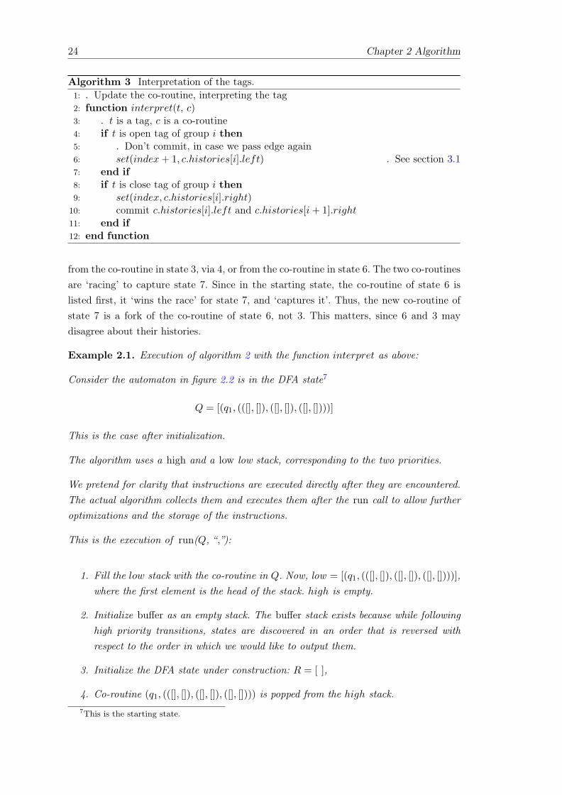
With this, the algorithm is simply implementing the fitting interpret function as seen inalgorithm 2.

The states are given to the algorithm in the order visited, so that the coroutine thatgot furthest is expanded first when the next character is read. The buffer variable is adetail that ensures that the correct order of co-routines is produced. If our procedure isconsistently used, the prioritization will lead to a correct match.

Note that the ordering of co-routines inside of DFA states is relevant. In figure 2.2, afterreading only one comma as an input, state 7 can be reached from two co-routines: either


Algorithm 3 Interpretation of the tags.1: . Update the co-routine, interpreting the tag2: function interpret(t, c)3: . t is a tag, c is a co-routine4: if t is open tag of group i then5: . Don’t commit, in case we pass edge again6: set(index+ 1, c.histories[i].left) . See section 3.17: end if8: if t is close tag of group i then9: set(index, c.histories[i].right)

10: commit c.histories[i].left and c.histories[i+ 1].right11: end if12: end function

from the co-routine in state 3, via 4, or from the co-routine in state 6. The two co-routinesare ‘racing’ to capture state 7. Since in the starting state, the co-routine of state 6 islisted first, it ‘wins the race’ for state 7, and ‘captures it’. Thus, the new co-routine ofstate 7 is a fork of the co-routine of state 6, not 3. This matters, since 6 and 3 maydisagree about their histories.

Example 2.1. Execution of algorithm 2 with the function interpret as above:

Consider the automaton in figure 2.2 is in the DFA state7

Q = [(q1, (([], []), ([], []), ([], [])))]

This is the case after initialization.

The algorithm uses a high and a low low stack, corresponding to the two priorities.

We pretend for clarity that instructions are executed directly after they are encountered.The actual algorithm collects them and executes them after the run call to allow furtheroptimizations and the storage of the instructions.

This is the execution of run(Q, “,”):

1. Fill the low stack with the co-routine in Q. Now, low = [(q1, (([], []), ([], []), ([], [])))],where the first element is the head of the stack. high is empty.

2. Initialize buffer as an empty stack. The buffer stack exists because while followinghigh priority transitions, states are discovered in an order that is reversed withrespect to the order in which we would like to output them.

3. Initialize the DFA state under construction: R = [ ],

4. Co-routine (q1, (([], []), ([], []), ([], []))) is popped from the high stack.7This is the starting state.


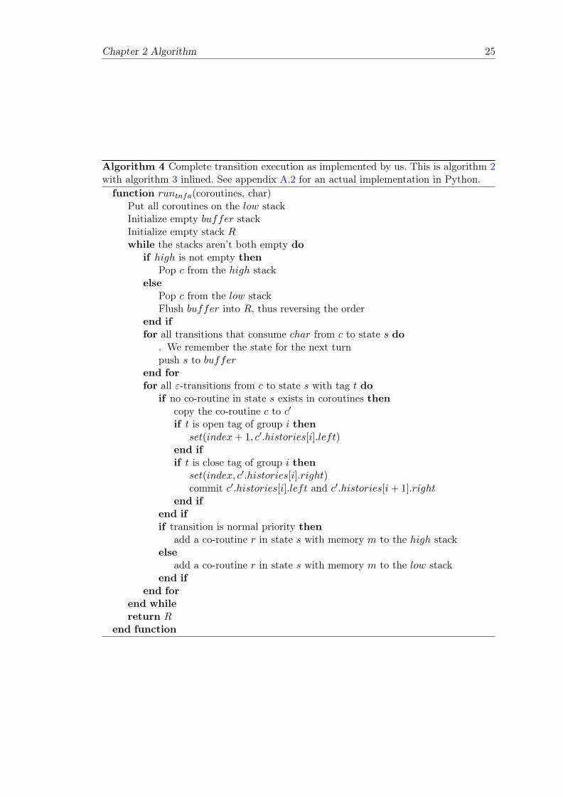
Algorithm 4 Complete transition execution as implemented by us. This is algorithm 2with algorithm 3 inlined. See appendix A.2 for an actual implementation in Python.function runtnfa(coroutines, char)

Put all coroutines on the low stackInitialize empty buffer stackInitialize empty stack Rwhile the stacks aren’t both empty do

if high is not empty thenPop c from the high stack

elsePop c from the low stackFlush buffer into R, thus reversing the order

end iffor all transitions that consume char from c to state s do

. We remember the state for the next turnpush s to buffer

end forfor all ε-transitions from c to state s with tag t do

if no co-routine in state s exists in coroutines thencopy the co-routine c to c′

if t is open tag of group i thenset(index+ 1, c′.histories[i].left)

end ifif t is close tag of group i then

set(index, c′.histories[i].right)commit c′.histories[i].left and c′.histories[i+ 1].right

end ifend ifif transition is normal priority then

add a co-routine r in state s with memory m to the high stackelse

add a co-routine r in state s with memory m to the low stackend if

end forend whilereturn R

end function


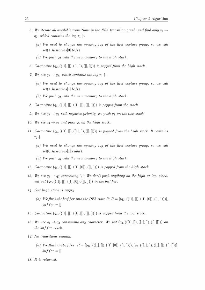
5. We iterate all available transitions in the NFA transition graph, and find only q1 →q2, which contains the tag τ1 ↑.

(a) We need to change the opening tag of the first capture group, so we callset(1, histories[0].left).

(b) We push q2 with the new memory to the high stack.

6. Co-routine (q2, (([1], []), ([], []), ([], []))) is popped from the high stack.

7. We see q2 → q3, which contains the tag τ2 ↑.

(a) We need to change the opening tag of the first capture group, so we callset(1, histories[1].left).


8. Co-routine (q3, (([1], []), ([1], []), ([], []))) is popped from the stack.

9. We see q3 → q4 with negative priority, we push q4 on the low stack.

10. We see q3 → q5 and push q5 on the high stack.

11. Co-routine (q5, (([1], []), ([1], []), ([], []))) is popped from the high stack. It containsτ2 ↓

(a) We need to change the opening tag of the first capture group, so we callset(0, histories[1].right).


12. Co-routine (q6, (([1], []), ([1], [0]), ([], []))) is popped from the high stack.

13. We see q6 → q7 consuming “,”. We don’t push anything on the high or low stack,but put (q7, (([1], []), ([1], [0]), ([], []))) in the buffer.

14. Our high stack is empty.

(a) We flush the buffer into the DFA state R: R = [(q7, (([1], []), ([1], [0]), ([], [])))],buffer = []

15. Co-routine (q4, (([1], []), ([1], []), ([], []))) is popped from the low stack.

16. We see q4 → q3 consuming any character. We put (q3, (([1], []), ([1], []), ([], []))) onthe buffer stack.

17. No transitions remain.

(a) We flush the buffer: R = [(q7, (([1], []), ([1], [0]), ([], []))), (q3, (([1], []), ([1], []), ([], []))],buffer = []

18. R is returned.


Some of the histories contain pairs of the kind ([1], [0]), which would be a group thatstarts after it began. This means that no character was matched, as can easily be checkedby comparing it to /((.∗?), (\d+)) + / on the string “,”.

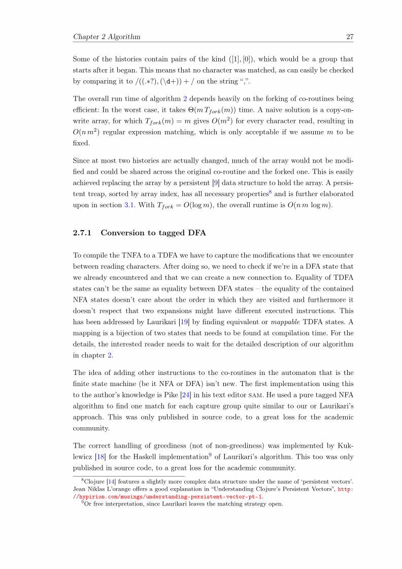
The overall run time of algorithm 2 depends heavily on the forking of co-routines beingefficient: In the worst case, it takes Θ(mTfork(m)) time. A naive solution is a copy-on-write array, for which Tfork(m) = m gives O(m2) for every character read, resulting inO(nm2) regular expression matching, which is only acceptable if we assume m to befixed.

Since at most two histories are actually changed, much of the array would not be modi-fied and could be shared across the original co-routine and the forked one. This is easilyachieved replacing the array by a persistent [9] data structure to hold the array. A persis-tent treap, sorted by array index, has all necessary properties8 and is further elaboratedupon in section 3.1. With Tfork = O(logm), the overall runtime is O(nm logm).

2.7.1 Conversion to tagged DFA

To compile the TNFA to a TDFA we have to capture the modifications that we encounterbetween reading characters. After doing so, we need to check if we’re in a DFA state thatwe already encountered and that we can create a new connection to. Equality of TDFAstates can’t be the same as equality between DFA states – the equality of the containedNFA states doesn’t care about the order in which they are visited and furthermore itdoesn’t respect that two expansions might have different executed instructions. Thishas been addressed by Laurikari [19] by finding equivalent or mappable TDFA states. Amapping is a bijection of two states that needs to be found at compilation time. For thedetails, the interested reader needs to wait for the detailed description of our algorithmin chapter 2.

The idea of adding other instructions to the co-routines in the automaton that is thefinite state machine (be it NFA or DFA) isn’t new. The first implementation using thisto the author’s knowledge is Pike [24] in his text editor sam. He used a pure tagged NFAalgorithm to find one match for each capture group quite similar to our or Laurikari’sapproach. This was only published in source code, to a great loss for the academiccommunity.

The correct handling of greediness (not of non-greediness) was implemented by Kuk-lewicz [18] for the Haskell implementation9 of Laurikari’s algorithm. This too was onlypublished in source code, to a great loss for the academic community.

8Clojure [14] features a slightly more complex data structure under the name of ‘persistent vectors’.Jean Niklas L’orange offers a good explanation in “Understanding Clojure’s Persistent Vectors”, http://hypirion.com/musings/understanding-persistent-vector-pt-1.

9Or free interpretation, since Laurikari leaves the matching strategy open.

http://hypirion.com/musings/understanding-persistent-vector-pt-1

http://hypirion.com/musings/understanding-persistent-vector-pt-1


Cox calls Laurikari’s TDFA a reinvention of Pike’s algorithm, but while that is in parttrue, Laurikari introduces the mapping step described in algorithm 7. This leads Lau-rikari’s algorithm to contain fewer states and one would hope that this would lead to abetter run-time than Google’s RE210, which is based on Pike’s algorithm.

This is not confirmed by the benchmarks by Sulzmann and Lu [27], but they offer anexplanation: in their profiling, they see that all Haskell implementations spend consider-able time decoding the input strings. In other words, the measured performance is moreof an artifact of the programming environment used.

Compared to RE2, our algorithm doesn’t provide many low-level optimizations, suchas limiting the TDFA cache size or an analysis of the pattern for common simplifica-tions such as optimizing for one-state matches11. Further it’s algorithm to simulate thebacktracking is simpler. However our algorithm doesn’t require a separate pass for matchdetection and match extraction, which opens different scenarios – the reason we can avoidthis is that we are able to collect the instructions and incorporate them into the lazyDFA state compilation. Our algorithm adds the mapping phase from Laurikari, whichallows us to find DFA states that can be made equivalent by some additional writes.

10https://code.google.com/p/re2/11unambiguous NFA can be interpreted as DFA and can be matched more efficiently

https://code.google.com/p/re2/

Chapter 3

Data structures

In the previous chapter, we obtained an algorithm with a run-time proportional to thecost of storing updates in a fixed size data structure with one access and one update.This needs to be fully persistent1 in order to allow for co-routine forking.

This chapter presents some possible data structures, that allow for this.

3.1 Fully persistent data structures

In order to allow modifications of our list of histories, it is necessary to build a datastructure that has the same interface as a copy-on-write array:

Definition 3.1. An Arraylike data structure A of length m must provide the followinginterface:

Constructor A(m) must return a structure of length m.

Random access An instance of A must provide a method get(i), which gives a historyfor each 0 ≤ i < m.

Setting elements An instance of A must provide a method set(i, history), which re-turns a new version of A, so that get(i) = history. The original instance must stillreturn the same value for any get and set – it must be logically unmodified.

This is a definition of a fixed-size fully-persistent linear data structure.

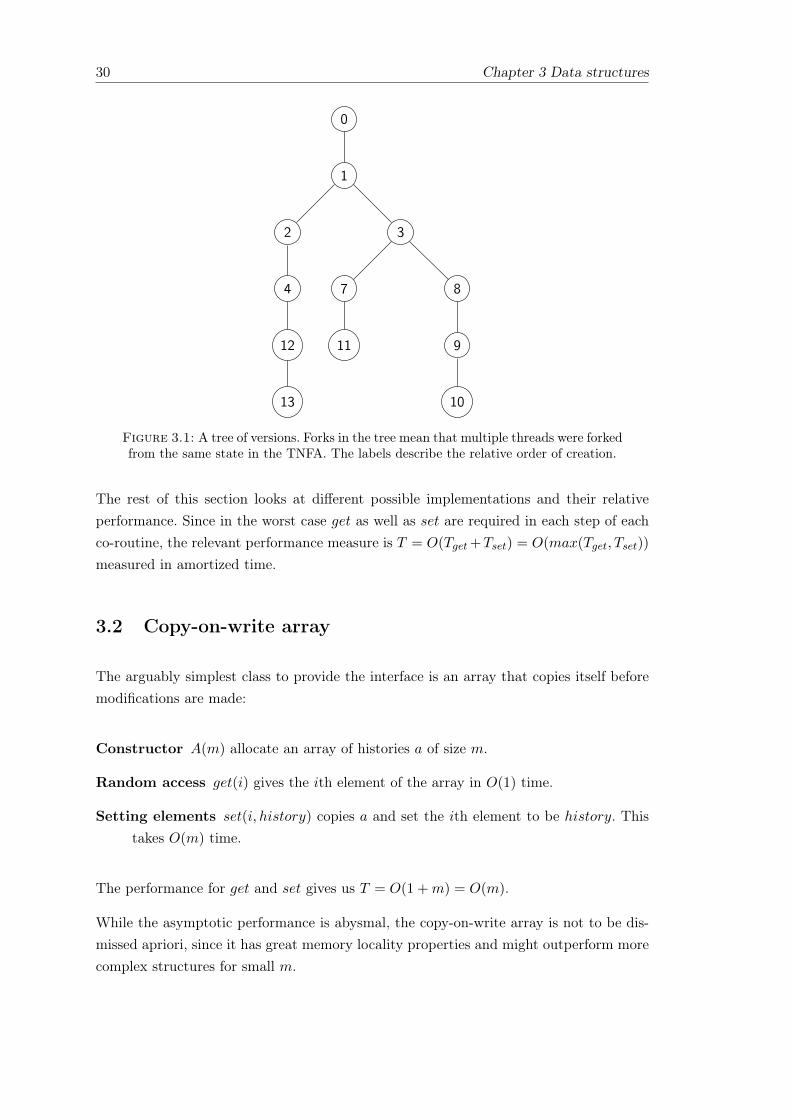
Every version that is in a living co-routine can change and so a single version can forkinto different directions. A way to visualize the history is as a tree of versions, whereeach set call forks off a new node, as seen in figure 3.1.

1This means that old versions of the data structure are still accessible and can be forked so that anew data structure with only that change applied can be accessed.

29

30 Chapter 3 Data structures

0

1

2

4

12

13

3

7

11

8

9

10

Figure 3.1: A tree of versions. Forks in the tree mean that multiple threads were forkedfrom the same state in the TNFA. The labels describe the relative order of creation.

The rest of this section looks at different possible implementations and their relativeperformance. Since in the worst case get as well as set are required in each step of eachco-routine, the relevant performance measure is T = O(Tget+Tset) = O(max(Tget, Tset))

measured in amortized time.

3.2 Copy-on-write array

The arguably simplest class to provide the interface is an array that copies itself beforemodifications are made:

Constructor A(m) allocate an array of histories a of size m.

Random access get(i) gives the ith element of the array in O(1) time.

Setting elements set(i, history) copies a and set the ith element to be history. Thistakes O(m) time.

The performance for get and set gives us T = O(1 +m) = O(m).

While the asymptotic performance is abysmal, the copy-on-write array is not to be dis-missed apriori, since it has great memory locality properties and might outperform morecomplex structures for small m.

Chapter 3 Data structures 31

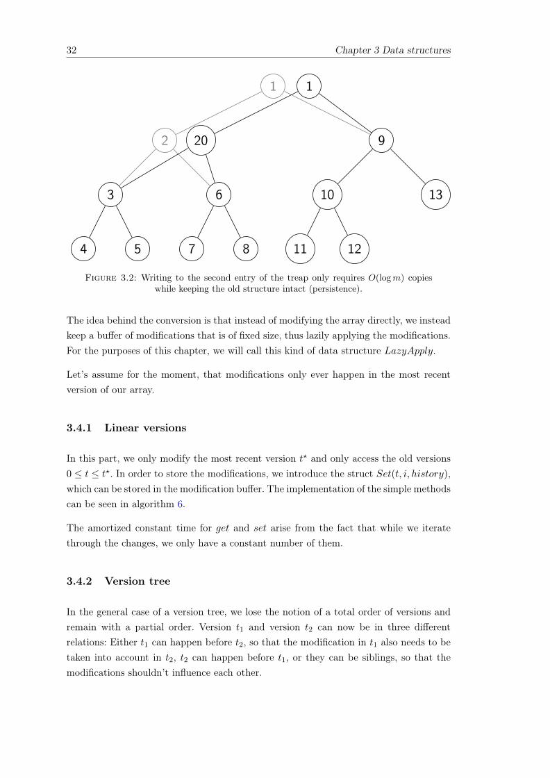
3.3 Treap

The treap data structure allows copy-on-write in logm time, sharing much of the struc-ture by using the flyweight pattern as can be seen in figure 3.2. The treap is a balanced,left-leaning binary tree with entries in each node, equipped with the operations get andset as follows.

Algorithm 5 Implementation of the treap methods1: function get(treap, index)2: if index = 0 then3: return treap.entry4: else if index− 1 < treap.left.size then5: return get(treap.left, index− 1)6: else7: return get(treap.right, index− treap.left.size− 1)8: end if9: end function

10: function set(treap, index, entry)11: if index = 0 then12: treap′ ← copy(treap)13: treap′.entry← entry14: return treap’15: else if index− 1 < treap.left.size then16: treap′ ← copy(treap)17: treap′.left← set(treap.left, index− 1, entry)18: return treap′

19: else20: treap′ ← copy(treap)21: treap′.left← set(treap.right, index− treap.left.size− 1, entry)22: return treap′

23: end if24: end function

This structure gives us better asymptotic performance at the cost of following logm

pointers, because T = O(logm+ logm) = O(logm).

3.4 Storing updates

Driscoll et al [9] describe how any pointer machine data structure with a fixed numberof links to each version can be converted to a fully persistent data structure in O(1)

amortized time. This section shows the steps involved to equip an array with such aninterface.


1

2

3

4 5

6

7 8

9

10

11 12

13

1

20

Figure 3.2: Writing to the second entry of the treap only requires O(logm) copieswhile keeping the old structure intact (persistence).

The idea behind the conversion is that instead of modifying the array directly, we insteadkeep a buffer of modifications that is of fixed size, thus lazily applying the modifications.For the purposes of this chapter, we will call this kind of data structure LazyApply.

Let’s assume for the moment, that modifications only ever happen in the most recentversion of our array.

3.4.1 Linear versions

In this part, we only modify the most recent version t? and only access the old versions0 ≤ t ≤ t?. In order to store the modifications, we introduce the struct Set(t, i, history),which can be stored in the modification buffer. The implementation of the simple methodscan be seen in algorithm 6.

The amortized constant time for get and set arise from the fact that while we iteratethrough the changes, we only have a constant number of them.

3.4.2 Version tree

In the general case of a version tree, we lose the notion of a total order of versions andremain with a partial order. Version t1 and version t2 can now be in three differentrelations: Either t1 can happen before t2, so that the modification in t1 also needs to betaken into account in t2, t2 can happen before t1, or they can be siblings, so that themodifications shouldn’t influence each other.


Algorithm 6 Methods of the LazyApply data structure1: function makeLazyApply(m)2: allocate an array of m histories hs3: allocate a buffer b of size p for modifications.4: return {histories : hs, buffer : b}5: end function6: function get(lazyApply, t, index)7: history ← lazyApply.histories[index]8: for each Set(t′, i, history′) do9: if t′ < t and i = index then

10: history ← history′

11: end if12: end for13: return history14: end function

15: function set(lazyApply, t, index, entry)16: if lazyApply.buffer has space left then17: add Set(t, index, entry) to lazyApply.buffer18: return lazyApply19: else20: return new LazyApply with all changes applied21: end if22: end function

The problem of generalizing this approach to version trees is twofold: The first problemis that we need to determine whether a modification applies to a version in constanttime, otherwise get would become slower. The second problem is that modifying thesame version reduces to copying the array of histories if said version has a full buffer.The latter is more easily solved and thus will be discussed first.

Emptying a full buffer Instead of applying all modifications, we can split the mod-ification buffer into two roughly equal parts. In order to do that, we can find a subtreev of modifications of size ≈ p

2 . Instead of applying all modifications to the array of his-tories, we only apply the ancestors of v. Then we delete all modifications in v from theoriginal node. Now we would be breaking the interface, because some co-routines stillhave references to the original node, but actually use a version that is in v. This canbe avoided by storing back-pointers to the threads and modify their references to thenew node if necessary. Since there are at most m threads referencing the versions of eachnode, we can still update the references in amortized constant time.

Constant time ordering of versions In order to determine whether to apply amodification on a read, we need to find the relation between the version that is queriedand the one that is stored. If tstored < tqueried, we apply the modification. This requires


us however to determine the relative positions of tstored and tqueried in the version tree,where the naive implementation would take logm time. This is the order maintenanceproblem and fittingly can be solved using an order maintenance data structure, such asthe one proposed by Dietz and Sleator [8] which we discuss in section 3.5.

For the moment let us assume that we have a linear data structure, that

1. allows an element to be inserted next to a known element in O(1) time.

2. allows us to query the order of two elements a and b in the list in O(1) time. We’llcall this operation query<(a, b).

With this we can flatten the tree to a list by adding a bt beginning element and an etclosing element to the list as seen in figure 3.3.

v1

v2

v3 v4

v5

(b1 (b2 (b3 e3) (b4 e4) e2) (b3 b3) e1)

Figure 3.3: A flattened version tree

Now we can find if version t2 depends on version t1, by calculating

query<(bt1 , bt2) && query<(et2 , et1)

If t1 encloses t2 completely, then t2 is part of the subtree of t1 and therefore we’d needto apply the modification at t1 to find values at t2.


3.5 Order maintenance

Dietz and Sleator describe in their paper Two Algorithms for Maintaining Order in aList [8]2, a simple one that provides amortized guarantees and a more involved one,which could offer worst-case guarantees. For our purposes the amortized version suffices,as noted by Driscoll et al [9, p. 108].

The data structure keeps so called tags η(e) for elements, which are integers that describethe order. In order to query the relative position of two elements, their tags are simplycompared, which leaves us with the problem of maintaining tags for all list elements suchthat η(e1) < η(e2)⇐ index(e1) < index(e2).

Compare this to the related problem of list-labeling: in order maintenance we need to beable to compute the full label for each element in constant time, whereas in list-labeling,the node has to contain the full label itself. This insight is key to maintaining order inamortized constant time. For the moment however we look at the method we can use forlist-labeling.

The key to achieve this is to use a doubly linked list of tags with their correspondingelements. If we need to insert an element after another known element e, we can insertit, but to keep our invariant, we assign η(enew) =

⌊η(e)+η(e.next)

2

⌋. This is possible, unless

the new tag is actually equal to η(e) – if η(e) doesn’t have any space to η(e.next). Inthis case we need to relabel the existing nodes.

3.5.1 Relabeling

The purpose of the relabeling step is to ensure that there is a gap to fit in the newelement and reduce the potential of a next reordering step. An intuitive perspective isshown by Bender et al [3]:

The labels can be thought of a coding of paths in a complete binary tree as visualizedin figure 3.4. We can then define the overflow in a subtree, which triggers relabeling.

Definition. The overflow threshold of a subtree is 1.5i for any level3 i, starting countingfrom the leaves, which are level 0.

Overflow happens, when the number of items in a subtree are bigger than the overflowthreshold.

With this definition, we can define the region that we relabel to be the first subtree thatisn’t in overflow – which means that is is filled sufficiently sparsely to reduce the potential

2And Bender et al[3] in their revision of this classical paper3a = 1.5 is an arbitrary choice for a number 1 < a < 2.


0002

0

0012

1

0

0102

0

0112

1

1

0

1002

0

1012

1

0

1102

0

1112

1

1

1

Figure 3.4: Labels are binary numbers describing paths in a tree. Relabeling walksup the tree until it finds a subtree with a density below the threshold. In this range,

the labels changed to make them equally spaced.

new relabels. In this subtree we spread the labels equally, which ensures that we will nothave to do any relabeling for another b1.5ic inserts. Note that a much bigger region mightbe in overflow, but no checks are done if they are not triggered by an overflow at level0, i.e. placing a node between two adjacent nodes.

This algorithm leaves us with the disappointment of only achieving O(logm) amortizedinsert. This can be resolved using a technique known as indirection.

3.5.2 Indirection

Indirection is a method introduced by Willard [29] to eliminate annoying log factorsunder certain conditions such as the one just encountered. With it we leave the realmof list-labeling and cease to store the full label in each node. Instead we now keep atwo-level structure as shown in figure 3.5.

Figure 3.5: Indirection structure: use a compound index with the high-order bits beingthe index for the upper structure and the low-order bits being the index for the lowerstructure. Since the upper index is stored in the summary structure, log u items can be

relabeled in O(1) time.

We split our universe into blocks of size Θ(log u). In these blocks we keep a labeledlist as seen in the previous section. Above this, we create a summary structure, whichstores a second part of the index. This too is a labeled list, but since each element of


the summary structure represents Θ(log u) elements of the universe, we can effectivelydo relabels faster by a log-factor. This gives us amortized O(1) updates.

It can be said that this seems to set a limit on the size of the match: Once our labels areused up, we cannot do O(1) order queries anymore. This is true, but there is a smallerlimit already in place: We can’t store pointers to a string that doesn’t fit into memory.If we cease to understand positions as fixed in size, we would again get a log-factor. Thisis typically not considered.

Chapter 4

Proofs

In this chapter we will prove the claimed properties, first and foremost the correctnessof the algorithm.

4.1 Correctness

The correctness of the algorithm follows by induction over the construction: If the cor-rect co-routine stops in the end state for all possible constructions of the Thompsonconstruction under the assumption that simpler automata do the same, it follows thatno matter how complex the automata get, the algorithm will have the correct output.

To this goal, we will use backtracking as a handy definition of correctness. We will showthat our algorithm will prefer the same paths as a backtracking implementation would.It should be noted that the construction is exactly set up so that it matches backtrackingand in fact this can be seen as a simple derivation of our algorithm.

First we need a simple formalization of the backtracking procedure:

39

40 Chapter 4 Proofs

bt(a|b, s) = bt(a, s) | bt(b, s)

bt(r∗, s) = bt(rr ∗ |ε, s)

bt(r∗?, s) = bt(ε|rr∗, s)

bt(r?, s) = bt(r|ε, s)

bt(r??, s) = bt(ε|r, s)

bt(r+, s) = bt(rr∗, s)

bt(r+?, s) = bt(rr∗?, s)

bt(ab, s) = bt(a, s) + bt(b, rest)

bt(Group(i, r), s) = [WriteOpen(i)] + bt(r, s) + [WriteClose(i)]

Second we notice that the algorithm preserves the order of the co-routines after eachcharacter read. This means that basically a depth first search is performed, with prioritiesformalizing what option is to be taken first.

The correct parse is found if and only if after reading the whole string,

1. the co-routine in the end state consumed all characters of the string (and onlythose) in order and

2. there is no co-routine that fulfills 1 that took “later” low-priority edges. This cor-responds to the depth-first search of backtracking.

That certain paths are cut off, because the state has already been seen is equivalent tomemoization in the backtracking procedure: If a higher priority state already found apath through this part of the parse, the following parse can be pruned.

There is the possibilities of circles, so that the depth-first solution would loop. This canbe seen for example in the regular expression /(a∗?) ∗ /, where the preferred route inthe graph is actually to capture an empty repetition of /a/. We tweak the Thompsonconstruction for this scenario, by giving a path to the logically next state after theautomaton with the same priority as from the start node for the star-operator, becauseit is the only automaton where the start state competes with a complete run throughthe pattern.

Now the parses are analogous for our procedure and bt:

Chapter 4 Proofs 41

bt(a|b, s):

1. Check a

2. Check b

1

2

b

-

a

1. Check 1→ a→ 2

2. Check 1→ b→ 2

bt(r∗, s):

1. Check r

2. Check ε

1

2

3

r

-

1. Check 1→ r → 2→ 1→ 3

2. Check 1→ 3

......

42 Chapter 4 Proofs

bt(ab, s):

1. Check a

2. Check b on rest

3. Concatenate the up-dates

1

2

b

a

1. Run through a consuming somecharacters

2. Run through b

3. All changes are written

bt(Group(i, r), s):

1. Write current positionto changes

2. Check r

3. Write position aftermatching r to changes

1

2

a

1. Write current position to changes

2. Run through r

3. Write the changed position tochanges

4.2 Execution time

The main structure of any NFA based matching algorithm is the nesting of two loops:The outer loop iterating over the n characters of the string, and the inner expandingat most m states. The expansion makes O(1) updates per state expanded, as the con-struction described in section 2.1 gives a constant out-degree for each state. As described

Chapter 4 Proofs 43

in chapter 3 the update cost of every co-routine is O(1). This gives a total run time ofO(nm).

4.3 Lower bound for time

There is no known tight1 lower bound to regular expression matching.

Theorem 1. No algorithm can correctly match regular expressions faster than Θ(n min(m, |Σ|)),where n is the length of the string, m is the length of the pattern, and |Σ| is the size ofthe alphabet.

Proof. Let S = anxi and R = [ax1] ∗ |[ax2] ∗ | . . . |[axm]∗. Note that |S| = Θn and |R| =Θ(min(m, |Σ|)). Let further match be a valid regular expression matching algorithm, then

match(S,R) is equivalent to finding anxi?∈ {anx1, . . . , anxm}. There is no particular

order to {anx1, . . . , anxm}, so the lower bound for finding this is Θ(|S| |R|).

1A lower bound l is tight, if it is the asymptotically largest lower bound

Chapter 5

Implementation

While repeatedly calling algorithm 2 would be sufficient to reach the theoretical timebound we claimed, practical performance can be dramatically improved by avoiding toconstruct new states. Instead, we build a transition table that maps from old DFA statesand an input range to a new DFA state, and the instructions to execute when using thetransition. We build the transition table, including instructions, as we go. This is whatwe mean when we say that the DFA is lazily compiled.

5.1 DFA transition table

The DFA transition table is different from the NFA transition table, in that the NFAtransition table contains ε transitions and may have more than one transition from onestate to another, for the same input range. DFA transition tables allow no ambiguity.

Our transition tables, both for NFAs and DFAs, assume a transition to map a consecu-tive range of characters. If, instead, we used individual characters, the table size wouldquickly become unwieldy. However, input ranges can quickly become confusing if theyare allowed to intersect. To avoid this, and simplify the code dramatically, while keepingthe transition table small, we use the following trick. When the regular expression isparsed, we keep track of all input ranges that occur in it. Then, we split them until notwo input ranges intersect. After this step, input ranges are never created again. Doingthis step early in the pipeline yields the following invariant: it is impossible to ever comeacross intersecting input ranges.

To give us a chance to ever be in a state that is already in the transition table, we check,after executing algorithm 2, run, whether there is a known DFA state that is mappableto the output of run. If run produced a DFA state Q, and there is a DFA state Q′ thatcontains the same NFA states, in the same order then Q and Q′ may be mappable. If theyare, then there is a set of instructions that move the histories from Q into Q′ such that,

45

46 Chapter 5 Implementation

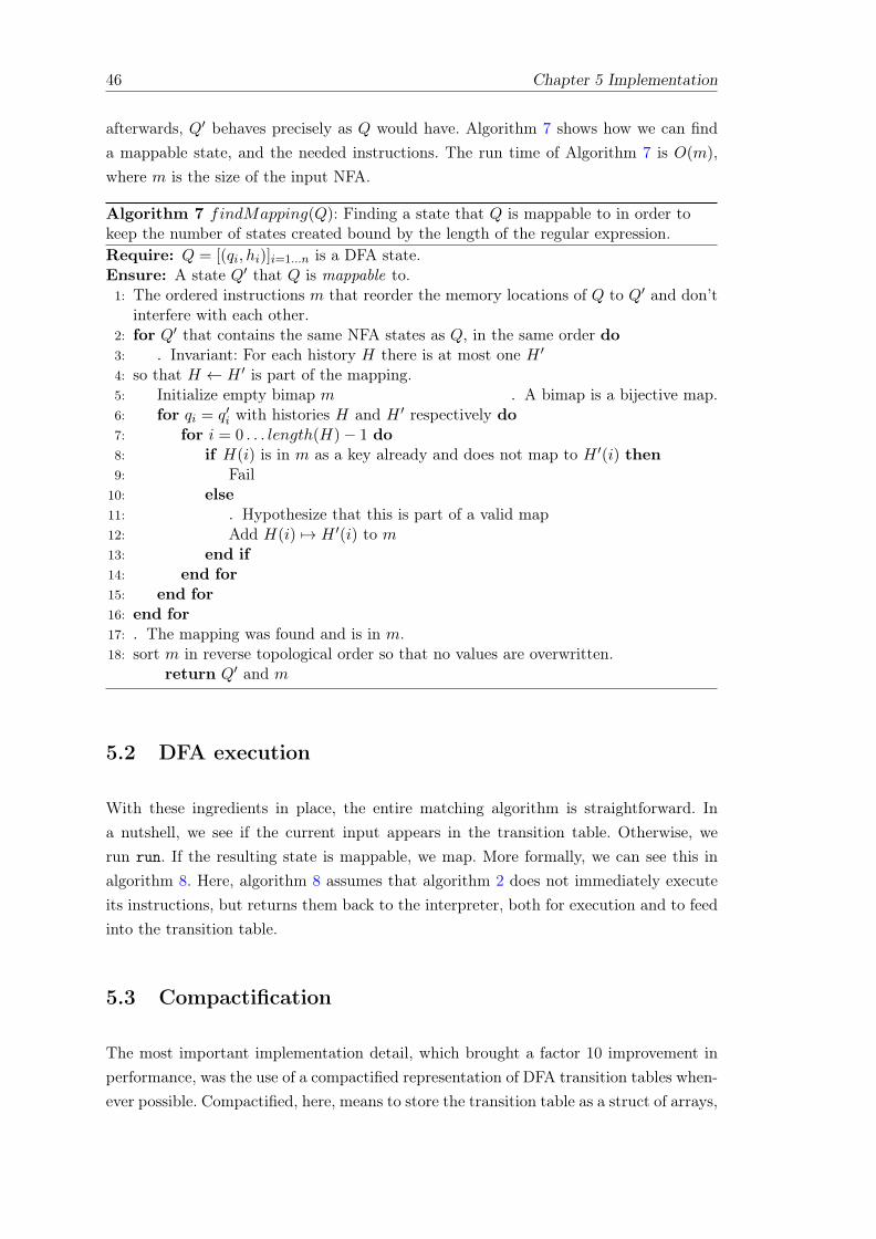
afterwards, Q′ behaves precisely as Q would have. Algorithm 7 shows how we can finda mappable state, and the needed instructions. The run time of Algorithm 7 is O(m),where m is the size of the input NFA.

Algorithm 7 findMapping(Q): Finding a state that Q is mappable to in order tokeep the number of states created bound by the length of the regular expression.Require: Q = [(qi, hi)]i=1...n is a DFA state.Ensure: A state Q′ that Q is mappable to.1: The ordered instructions m that reorder the memory locations of Q to Q′ and don’t

interfere with each other.2: for Q′ that contains the same NFA states as Q, in the same order do3: . Invariant: For each history H there is at most one H ′

4: so that H ← H ′ is part of the mapping.5: Initialize empty bimap m . A bimap is a bijective map.6: for qi = q′i with histories H and H ′ respectively do7: for i = 0 . . . length(H)− 1 do8: if H(i) is in m as a key already and does not map to H ′(i) then9: Fail

10: else11: . Hypothesize that this is part of a valid map12: Add H(i) 7→ H ′(i) to m13: end if14: end for15: end for16: end for17: . The mapping was found and is in m.18: sort m in reverse topological order so that no values are overwritten.

return Q′ and m

5.2 DFA execution

With these ingredients in place, the entire matching algorithm is straightforward. Ina nutshell, we see if the current input appears in the transition table. Otherwise, werun run. If the resulting state is mappable, we map. More formally, we can see this inalgorithm 8. Here, algorithm 8 assumes that algorithm 2 does not immediately executeits instructions, but returns them back to the interpreter, both for execution and to feedinto the transition table.

5.3 Compactification

The most important implementation detail, which brought a factor 10 improvement inperformance, was the use of a compactified representation of DFA transition tables when-ever possible. Compactified, here, means to store the transition table as a struct of arrays,

Chapter 5 Implementation 47

Algorithm 8 interpret(input): Interpretation and lazy compilation of the NFA. Seeappendix A.2 for an implementation in PythonRequire: input is a sequence of characters.Ensure: A tree of matching capture groups.1: . Lazily compiles a DFA while matching.2: Set Q to startState.3: . A co-routine is an NFA state, with an array of histories.4: Let Q be all co-routines that are reachable in the NFA transition graph by followingε transitions only.

5: Execute instructions described in algorithm run, when walking ε transitions.6: . Create the transition map of the DFA.7: Set T to an empty map from state and input to new state and instructions.8: . Consume string9: for position pos in input do

10: Let a be the character at position pos in input.11: if T has an entry for Q and a then12: . Let the DFA handle a13: Read the instructions and new state Q′ out of T14: execute the instructions15: Q← Q′

16: jump back to start of for loop.17: else18: . lazily compile another DFA state.19: Run run(Q, a) to find new state Q′ and instructions20: Run findMapping(Q′, T ) to see if Q’ can be mapped to an existing state Q′′

21: if Q′′ was found then22: Append the mapping instructions from findMapping to the instructions

found by run23: Execute the instructions.24: Add an entry to T , from current state Q and a, to new state Q′′ and

instructions.25: Set Q to Q′′

26: else27: Execute the instructions found by run.28: Add an entry to T , from current state Q and a, to new state Q′ and

instructions.29: Set Q to Q′.30: end if31: end if32: end for

48 Chapter 5 Implementation

rather than as an array of structs, as recommended by the Intel optimization handbook[4, section 6.5.1]. The transition table is a map from source state and input range totarget state and instructions. Following Intel’s recommendation, we store it as an ob-ject of five arrays: int[] oldStates, char[] froms, char[] tos, Instruction[][]

instructions, int[] newStates, all of the same length, such that the ith entry in thetable maps from oldStates[i], for a character greater than from[i], but smaller than to[i],to newStates[i], by executing instructions[i]. To read a character, the engine now searchesin the transition table, using binary search, for the current state and the current inputcharacter, executes the instructions it finds, and transitions to the new state.

However, the above structure isn’t a great fit with lazy compilation, as new transitionsmight have to be added into the middle of the table at any time. Another problem is that,above, the state is represented as an integer. However, as described in the algorithm, aDFA state is really a list of co-routines. If we need to lazily compile another DFA state,all of the co-routines need to be examined.

The compromise we found is the following: The canonical representation of the transitiontable is a red-black tree of transitions, each transition containing source and target DFAstate (both as the full list of their NFA states, and histories), an input range, and alist of instructions. This structure allows for quick insertion of new DFA states oncethey are lazily compiled. At the same time, lookups in a red-black tree are logarithmic.Then, whenever we read a fixed number of input characters without lazily compiling,we transform the transition table to the struct of arrays described above, and switch tousing it as our new transition table. If, however, we read a character for which there is notransition, we need to de-optimize, throw away the compactified representation, generatethe missing DFA state, and add it to the red-black tree.

The above algorithm chimes well with the observation that usually, regular expressionmatching needs only a handful of DFA states, and thus, compactification can be doneearly, and only seldom need to be undone.

5.4 Intertwining of the pipeline stages

The lazy compilation of the DFA when matching a string enables us to avoid compilingstates of it that might never be needed. This allows us to avoid the full power setconstruction [26], which has time complexity of O(2m), where m is the size of the NFA.

5.5 Parsing the regular expression syntax

Parsing the regular expression into an abstract syntax tree is a detail that can easily bemissed. Since the algorithm for matching is already very fast, preliminary experiments

Chapter 5 Implementation 49

abcdab|cd

a*b?|c*?d*?

(a+ (a?b(c*?)))

(.*?(.*?\.)*([A

-Z] [a-zA-Z]* ))* .*?

102

103

104

105

106

107

pa

rse

tim

e i

n n

sparsec

new

Figure 5.1: Comparison of two ways of parsing the regular expression syntax. Since themeasurements are very noisy, the median with the MAD (median absolute deviation)

are plotted.

showed that the parsing of the regular expression, even in simple regular expressions,can take up a major part (25% in our experiment) of the time for running the completematch.

The memory model to parse a regular expression is a stack, since capture groups can benested. The grammar can be formulated as right recursive and with this formulation itcan be implemented with a simple recursive descent parser as opposed to the previousParsec parser. The resulting parser eliminated the parsing of the regular expression as abottleneck, as can be seen in figure figure 5.1 (note the log plot).

Chapter 6

Related work

While there is no shortage of books discussing the usage of regular expressions, theimplementation side of regular expression has not been so lucky. Cox is spot-on whenhe argues that innovations have repeatedly been ignored and later reinvented [5, 6, 7],in part, not least because the publication medium of source code without accompanyingarticle was chosen.

Regular expressions are by no means new and originated with Kleene in the 1950 [26].This chapter first introduces some standard procedures for regular expression matching(without extracting any information), such as Backtracking in section 1.4 and variousautomata based approaches in sections 2.1, 2.2, and 2.3. In section 2.4 we discuss anaddition to the automata based approaches called tags that allows for the extraction ofsub-matches. We show that backtracking based approaches are not the straw man thatone could believe them to be in section 6.1. Even though we first believed ourselves tobe, we are actually not the first to produce parse trees in competitive time, as seen insection 6.3.

A problematic aspect of the literature is that many authors perceive regular expressionparsing to be a linear problem – linear in the length of the string with a constant forthe pattern size. This limits the applications, because this means that an algorithm thattakes O(2m+n) time seems very competitive for a small and fixed m, but is prohibitivelyexpensive for large m. The argument that the pattern is typically small seems circularto the author, because would the implementation focus on allowing large patterns, newapplications using large patterns would arise1.

In this paper, we will consider the best known algorithms to be quadratic. It is notknown if there is any algorithm that beats the O(nm) matching, but in section 4.3, alower bound of Θ(n min(m, |Σ|)) is proven.

1To check if a document contains features f1, f2, . . . , fn, we would match the document against regularexpression /(f1)|(f2)| . . . |(fn)/.

51

52 Chapter 6 Related work

6.1 Revisiting backtracking

As seen earlier, backtracking makes for easy implementations, but exponential run-timein the worst case for many patterns. Norvig [23] showed that this can be avoided by usingmemoization for context free grammars. This allows for O(n3m) time parsing. While thisis significantly higher than the O(nm) of the automata based approaches, it is also moregeneral, because more than just regular grammars can be parsed with this approach.This approach is taken by combinatoric parsers such as the Parsec library2. It should benoted however that while this approach has been known for some time now and promisesexponential speed-up, it is by no means a standard optimization for backtracking basedregular expression implementations.

First let us recapitulate what memoization means: For a function f we can create amemoized function f̂ such that

Initialize hash map cachefunction f̂(*args)

if args not in cache thenval← f(∗args)cache[args] = val

end ifreturn cache[args]

end function

This means that repeatedly calling the same function with the same inputs only costslookup time after the function has been evaluated once.

The parser presented by Norvig inherently produces parse trees, because it tries to reducethe list of tokens into all possible expansions of the base symbol. For example /a ∗ a ∗ /would be converted to a grammar

A → a

ASTAR → A ASTARASTAR → ε

FULL → ASTAR ASTAR

Now we can memoize the result for a non-terminal symbol and the remainder of thestring, which avoids exponentially many trial and error parses.

The same arguments that make this efficient for context-free grammars however alsomake the memoization approach applicable to the backtracking algorithm for regularexpressions.

2The memoization stems from the common subexpression optimization of Haskell

Chapter 6 Related work 53

To see the advantage, let’s revise the example that produced exponential runtime forregular backtracking: /(x∗) ∗ y/ on the string xn. Now consider

b̂t(xn, /(x∗) ∗ y/) = b̂t(xn, /(x∗)(x∗) ∗ y/)︸︷︷︸1 repetition

|| b̂t(xn, /y/)

= b̂t(xn−1, /(x∗)(x∗) ∗ y/) || b̂t(xn, /(x∗) ∗ y/) || b̂t(xn, /y/)

= . . .

= b̂t(x0, /(x∗)(x∗) ∗ y/) || b̂t(x1, /(x∗) ∗ y/) || . . .

|| b̂t(xn, /(x∗) ∗ y/) || b̂t(xn, /y/)

= b̂t(x1, /(x∗) ∗ y/) || . . . || b̂t(xn, /(x∗) ∗ y/) || b̂t(xn, /y/)

= b̂t(x1, /y/) || b̂t(x1, /(x∗)(x∗) ∗ y/)︸︷︷︸memoized

|| . . .

|| b̂t(xn, /(x∗) ∗ y/) || b̂t(xn, /y/)

= . . .

= b̂t(xn, /y/)

= no match

Nearly all backtracking can be avoided, because the branch has been evaluated before.

6.2 Packrat parsers

The memoization approach can be extended further to so-called packrat parsing [20]based on Parsing Expression Grammars (PEG), to obtain O(nm), but the memoizationgives a space overhead that is O(n), with a big constant [11] – or to put it in anotherway: The original string is stored several times over. This makes them flexible and fastparsers for small input, but they cannot be used for big data sets. To understand howthey work, let’s first look at PEG:

Parsing Expression Grammars are grammars similar to context-free grammars with thedifference that they allow no left-recursion and no ambiguity each expression has exactlyone correct parse tree and consumes at least one character. In this they are similar toregular expressions, but capture more than just regular languages. Such an expression cancontain literals, recursive subexpressions, ordered choice, repetitions and non-consumingpredicates:

recursive subexpressions allow for recursive repetition of a pattern, for example

S→ ′(′ S ′)′ /ε


orS→ ′if′ P ′{′ S ′}′

ordered choice gives two options, but the left path will be checked first and if itmatches already, the right path will not even be considered.

repetitions The operators *, +, and ? with their meaning identical to their usage inregular expressions.

non-consuming predicates The operator & will only match and return the left-handside, if the right-hand side would also match. The right-hand side doesn’t consumeany characters however. Similarly the operator ! only matches the left-hand side,if the right-hand side does not match (without consuming any characters for theright-hand side).

The implementation of these grammars as recursive descent/backtracking parsers is quitesimple. The corresponding Packrat parser is the straight forward memoization of this.This is in principle nothing new, the memoization approach to context-free grammars usesthe same approach, but the restriction to PEG simplify the problem: without ambiguityfewer references need to be stored to possible parses and since parsers consume at leasta character, each character in the input string has at most m possible interpretations.

The downside to this is that Packrat parsers have a large space overhead that make theminfeasible for large inputs [2]3.

6.3 Automata based extraction of parse trees

Memoization is a powerful tool to achieve fast parsers, but they have a space-overheadin order of the input instead of the parse tree size. The other approach to parsing – finitestate automata – offers a remedy. These approaches, one of which will be presented inthis paper, use tagged finite state automata that store the parse tree in some manner, themain differences being the format of the stored tree and the type of automaton runningthe parse.

The rivaling memory layouts are lists of changes and an array with a cell for each group.The former makes it hard to compile the TNFA to a TDFA with aggressive reuse ofstates via mapping (as described in algorithm 7), but has lower space consumption. Themapping in terms of cells for each group is easy, but costs a factor m space overhead.

3

“The Java parser generated by Pappy requires up to 400 bytes of memory for every byteof input.”

Chapter 6 Related work 55

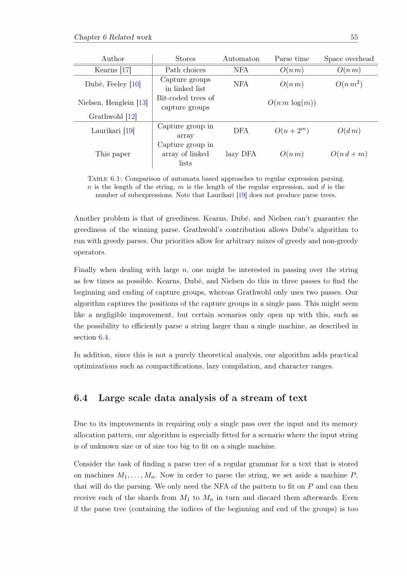
Author Stores Automaton Parse time Space overheadKearns [17] Path choices NFA O(nm) O(nm)

Dubé, Feeley [10] Capture groupsin linked list NFA O(nm) O(nm2)

Nielsen, Henglein [13] Bit-coded trees ofcapture groups O(nm log(m))

Grathwohl [12]

Laurikari [19] Capture group inarray DFA O(n+ 2m) O(dm)

This paperCapture group inarray of linked

listslazy DFA O(nm) O(nd+m)

Table 6.1: Comparison of automata based approaches to regular expression parsing.n is the length of the string, m is the length of the regular expression, and d is the

number of subexpressions. Note that Laurikari [19] does not produce parse trees.

Another problem is that of greediness. Kearns, Dubé, and Nielsen can’t guarantee thegreediness of the winning parse. Grathwohl’s contribution allows Dubé’s algorithm torun with greedy parses. Our priorities allow for arbitrary mixes of greedy and non-greedyoperators.

Finally when dealing with large n, one might be interested in passing over the stringas few times as possible. Kearns, Dubé, and Nielsen do this in three passes to find thebeginning and ending of capture groups, whereas Grathwohl only uses two passes. Ouralgorithm captures the positions of the capture groups in a single pass. This might seemlike a negligible improvement, but certain scenarios only open up with this, such asthe possibility to efficiently parse a string larger than a single machine, as described insection 6.4.

In addition, since this is not a purely theoretical analysis, our algorithm adds practicaloptimizations such as compactifications, lazy compilation, and character ranges.

6.4 Large scale data analysis of a stream of text

Due to its improvements in requiring only a single pass over the input and its memoryallocation pattern, our algorithm is especially fitted for a scenario where the input stringis of unknown size or of size too big to fit on a single machine.

Consider the task of finding a parse tree of a regular grammar for a text that is storedon machines M1, . . . ,Mn. Now in order to parse the string, we set aside a machine P ,that will do the parsing. We only need the NFA of the pattern to fit on P and can thenreceive each of the shards from M1 to Mn in turn and discard them afterwards. Evenif the parse tree (containing the indices of the beginning and end of the groups) is too


large to fit on the machine, we can send the cells to other machines. Because the cellsare not touched anymore, there will never be a need for P to retrieve old cells.

Chapter 7

Benchmark

All benchmarks were obtained using Google’s caliper1, which takes care of the most obvi-ous benchmarking blunders. It runs a warm-up before measuring, runs all experiments inseparate VMs, helps circumvent dead-code detection by accepting the output of dummyvariables as input, and fails if compilation occurs during experiment evaluation. Thesource code of all benchmarks is available, together with the sources of the project, onGithub. We ran all benchmarks on a 2.3 GHz, i7 Macbook Pro.

As we saw in section 6, there is a surprising dearth of regular expression engines thatcan extract nested capture groups – never mind extracting entire parse trees – that donot backtrack. Back-tracking implementations are exponential in their run-time, andso we see in figure 7.1 (note the log plot) how the run-time of “java.util.regex” quicklyexplodes exponentially, even for tiny input, for a pathological regular expression, whileour approach slows down only linearly. The raw data is seen in table 7.1.

n 13 14 15 16 17 18 19 20

java.util.regex 241 484 1003 1874 3555 7381 14561 30116Our implementation 225 252 273 32 327 352 400 421

Table 7.1: Matching times, in microseconds, for matching a?nan against input an.

In the opposite case, in the case of a regular expression that’s crafted to prevent anyback-tracking, java.util.regex outperforms our approach by more than factor 2, as seenin table 7.2 – but bear in mind that java.util.regex does not extract parse trees, but onlythe last match of all capture groups. A backtracking implementation that actually doesproduce complete parse trees is JParsec2, which, as also seen in table 7.2, performs onpar with our approach.

1https://code.google.com/p/caliper/2http://jparsec.codehaus.org

57

https://code.google.com/p/caliper/

http://jparsec.codehaus.org

58 Chapter 7 Benchmark

time

n

Figure 7.1: Time in nanoseconds for matching a?nan against input an. Bottom (pur-ple) line is our approach, top (blue) line is java.util.regex.

Note that because java.util.regex achieves its back-tracking through recursion, we hadto set the JVM’s stack size to one Gigabyte for it to parse the input. Since default stacksize is only a few megabytes, this makes using java.util.regex a security risk, even forunproblematic regular expressions that cannot cause backtracking, since an attacker canpotentially force the VM to run out of stack space.

Tool Time

JParsec 4,498java.util.regex 1,992

Ours 5,332

Table 7.2: Matching regular expression /((a + b) + c) + / against input (a200bc)2000,where a200 denotes 200 times character ‘a’. Time in microseconds.

Finally, a more realistic example, neither chosen to favor back-tracking nor to avoid it,extracts all class names, with their package names, from the project sources itself. Asseen in table 7.3, our approach outperforms java.util.regex by 40%, even though ourapproach constructs the entire parse tree, and thus all class names, while java.util.regexoutputs only the last matched class name. JParsec was not included in this experiment,since it does not allow non-greedy matches. Even though it is possible to build a parserthat produces the same AST, it would necessarily look very different (using negation)from the regular expression.

Chapter 7 Benchmark 59

Tool Time

java.util.regex 11,319Ours 8,047

Table 7.3: Runtimes, in microseconds, for finding all java class namesin all .java files in the project itself. The regular expression used is

/(.∗?([a− z] + \.) ∗ ([A− Z][a− zA− Z]∗)) ∗ .∗?/. Runtime in microseconds

Chapter 8

Conclusion

Regular expressions make for lightweight parsers and there are many cases where datais extracted this way. If such data is structured instead of flat, a parser that producestrees is superior to a standard regular expression parser. We provide such an algorithmwith modern optimizations applied using results from persistent data-structures to avoidunnecessary memory consumption and the slow-down that this would produce. This algo-rithm is able to provide the same semantics as backtracking, but without an exponentialworst case.

Our approach can produce entire parse trees from matching regular expressions in asingle pass over the string and do so asymptotically no slower than regular expressionmatching without any extraction. The practical performance is on par with traditionalback-tracking solutions if no backtracking ever happens, exponentially outperforms back-tracking approaches for pathological input, and in a realistic scenario outperforms back-tracking by 40%, even though our approach produces the full parse tree, and the back-tracking implementation doesn’t. All source code and all benchmarks are available undera free license on Github [22] at https://github.com/nes1983/tree-regex.

61

https://github.com/nes1983/tree-regex

Appendices

63

Appendix A

Minimal python implementation

This chapter shows a small implementation of our TNFA interpretation algorithm writtenin Python:

A.1 Construction

This doesn’t include the parsing of the regular expression grammar, but instead con-structs the automaton from an S-expression.

from itertools import count

def add_eps(table , start , goal , tag=None):table.setdefault(start , {}). setdefault(None , []). append ((goal , tag))assert (len(list(u for u, x in table[start ][None] if x != ’-’))

in (0,1)), ("Too many non -prioritized edges in %s: %s\n\n%s" %

(start , table[start ][None], table))

def construct(expression , table , start , end , counter ,outer=False):

if not expression:return table , start , end

(op , args) = expressionif op == ’seq’:

iter_start = startiter_end = next(counter)for x in args:

construct(x, table , iter_start , iter_end , counter)iter_start = iter_enditer_end = next(counter)

add_eps(table , iter_start , end)if op == ’lit’:

iter_start = startiter_end = next(counter)for l in args:

table.setdefault(iter_start , {})[l] = iter_enditer_start = iter_end

65

66 Appendix A Minimal python implementation

iter_end = next(counter)add_eps(table , iter_start , end)

if op == ’*’:up = next(counter)done = next(counter)construct(args[0], table , up , done , counter)add_eps(table , start , up)add_eps(table , done , start)add_eps(table , start , end , ’-’)add_eps(table , done , end , ’-’)

if op == ’*?’:up = next(counter)construct(args[0], table , up , start , counter)add_eps(table , start , up, ’-’)add_eps(table , start , end)

if op == ’?’:middle = next(counter)construct(args[0], table , middle , end , counter)add_eps(table , start , end , ’-’)add_eps(table , start , middle)

if op == ’??’:middle = next(counter)construct(args[0], table , middle , end , counter)add_eps(table , start , middle , ’-’)add_eps(table , start , end)

if op == ’group’:sstart = next(counter)eend = next(counter)group , exp = argsconstruct(exp , table , sstart , eend , counter)add_eps(table , start , sstart , (group , ’l’))add_eps(table , eend , end , (group , ’r’))

if outer:end_of_string = next(counter)table.setdefault(end , {})[’\0’] = end_of_stringend = end_of_string

return table , start , end

def seq(*e):return (’seq’, e)

def group(i, e):return (’group’, [i, e])

def star(e):return (’*’, [e])

def nstar(e):return (’*?’, [e])

def lit(e):return (’lit’, e)

def opt(e):return (’?’, [e])

def nopt(e):

Appendix A Minimal python implementation 67

return (’??’, [e])

A.2 Matching

import copy

def consume(tnfa , start , c, i):low = list(reversed(start ))high = []R = []seen = set()buffer = []while low or high:

if not high:e = low.pop()high.append(e)R.extend(buffer)buffer = []continue

state , mem = high.pop()if state in seen:

continueseen.add(state)transitions = tnfa.get(state , {})consuming = transitions.get(c)if consuming:

R.append ((cons , mem))epsilon = transitions.get(None)if not epsilon: continuefor (s, tag) in epsilon:

if tag == ’-’:low.append ((s, mem))continue

if tag:n, side = tagmem = copy.deepcopy(mem)mem.setdefault(n, ([], []))[0 if side == ’l’ else 1]. append(

i if side == ’r’ else i+1)high.append ((s, mem))

R.extend(buffer)return R

def match(regex , string ):counter = count ()

tnfa , start , end = construct(regex , {}, next(counter), next(counter), counter , outer=True)

ran = [(start , {})]for i, c in enumerate(string + ’\0’):

ran = consume(tnfa , ran , c, i)

return dict(ran).get(end)

Bibliography

[1] Arvind Arasu, Surajit Chaudhuri, Zhimin Chen, Kris Ganjam, Raghav Kaushik,and Vivek R. Narasayya. Experiences with using data cleaning technology for bingservices. IEEE Data Eng. Bull., 35(2):14–23, 2012.

[2] Ralph Becket and Zoltan Somogyi. DCGs + Memoing = Packrat parsing, but is itworth it? In Practical Aspects of Declarative Languages, volume LNCS 4902, pages182–196. Springer, January 2008.

[3] Michael A Bender, Richard Cole, Erik D Demaine, Martin Farach-Colton, and JackZito. Two simplified algorithms for maintaining order in a list. In Algorithms—ESA2002, pages 152–164. Springer, 2002.

[4] Intel Coorporation. Intel 64 and ia-32 architectures optimization reference manual,2013.

[5] R. Cox. Regular expression matching can be simple and fast (but is slow in java,perl, php, python, ruby,...). URL: http://swtch.com/˜rsc/regexp/regexp1.html, 2007.

[6] R. Cox. Regular expression matching: the virtual machine approach. URL:http://swtch.com/˜rsc/regexp/regexp2.html, 2009.

[7] R. Cox. Regular expression matching in the wild. URL:http://swtch.com/˜rsc/regexp/regexp3.html, 2010.

[8] Paul Dietz and Daniel Sleator. Two algorithms for maintaining order in a list.In Proceedings of the nineteenth annual ACM symposium on Theory of computing,pages 365–372. ACM, 1987.

[9] James R. Driscoll, Neil Sarnak, Daniel D. Sleator, and Robert E. Tarjan. Makingdata structures persistent. Journal of Computer and System Sciences, 38(1):86–124,February 1989.

[10] Danny Dubé and Marc Feeley. Efficiently building a parse tree from a regularexpression. Acta Informatica, 37(2):121–144, 2000.

[11] Bryan Ford. Packrat parsing: simple, powerful, lazy, linear time, functional pearl.In ICFP 02: Proceedings of the seventh ACM SIGPLAN international conferenceon Functional programming, volume 37/9, pages 36–47, New York, NY, USA, 2002.ACM.

69

70 BIBLIOGRAPHY

[12] Niels Bjørn Bugge Grathwohl, Fritz Henglein, Lasse Nielsen, and Ulrik Terp Ras-mussen. Two-pass greedy regular expression parsing. In Implementation and Appli-cation of Automata, pages 60–71. Springer, 2013.

[13] Fritz Henglein and Lasse Nielsen. Regular expression containment: coinductive ax-iomatization and computational interpretation. In ACM SIGPLAN Notices, vol-ume 46, pages 385–398. ACM, 2011.

[14] Rich Hickey. The Clojure programming language. In DLS ’08: Proceedings of the2008 symposium on Dynamic languages, pages 1–1, New York, NY, USA, 2008.ACM.

[15] Adam Jacobs. The pathologies of big data. Commun. ACM, 52(8):36–44, August2009.

[16] L. Karttunen, J. P. Chanod, G. Grefenstette, A. Schiller, and Received February.Regular expressions for language engineering. In Natural Language Engineering,pages 305–328, 1996.

[17] Steven M Kearns. Extending regular expressions with context operators and parseextraction. Software: Practice and Experience, 21(8):787–804, 1991.

[18] Chris Kuklewicz. Regular expressions/bounded space proposal, February 2007.

[19] V. Laurikari. Nfas with tagged transitions, their conversion to deterministic au-tomata and application to regular expressions. In String Processing and Informa-tion Retrieval, 2000. SPIRE 2000. Proceedings. Seventh International Symposiumon, pages 181–187. IEEE, 2000.

[20] Sérgio Medeiros, Fabio Mascarenhas, and Roberto Ierusalimschy. From regexes toparsing expression grammars. Science of Computer Programming, 2012.

[21] Chad R. Meiners, Jignesh Patel, Eric Norige, Eric Torng, and Alex X. Liu. Fastregular expression matching using small TCAMs for network intrusion detectionand prevention systems. In Proceedings of the 19th USENIX conference on Security,USENIX Security’10, page 8, Berkeley, CA, USA, 2010. USENIX Association.

[22] Aaron Karper Niko Schwarz. O(n m) regular expression parsing library that pro-duces parse trees, 2014.

[23] Peter Norvig. Techniques for automatic memoization with applications to context-free parsing. Computational Linguistics, 17(1):91–98, 1991.

[24] R. Pike. The text editor sam. Software: Practice and Experience, 17(11):813–845,1987.

[25] Robert Sedgewick. Algorithms in C (paperback). Addison-Wesley Professional, 1edition, January 1990.

[26] Michael Sipser. Introduction to the Theory of Computation. Course Technology, 2edition, February 2005.

BIBLIOGRAPHY 71

[27] M. Sulzmann and K.Z.M. Lu. Regular expression sub-matching using partial deriva-tives. In Proceedings of the 14th symposium on Principles and practice of declarativeprogramming, pages 79–90. ACM, 2012.

[28] Ken Thompson. Programming techniques: Regular expression search algorithm.Commun. ACM, 11(6):419–422, June 1968.

[29] Dan E Willard. Maintaining dense sequential files in a dynamic environment. InProceedings of the fourteenth annual ACM symposium on Theory of computing, pages114–121. ACM, 1982.

List of Figures

1.1 Posix parse tree . . . . . . . . . . . . . . . . . . . . . . . . . . . . . . . . . 71.2 Full parse tree . . . . . . . . . . . . . . . . . . . . . . . . . . . . . . . . . . 8

2.1 Thompson construction . . . . . . . . . . . . . . . . . . . . . . . . . . . . 162.2 NFA for /((.∗?), (\d+); ) + / . . . . . . . . . . . . . . . . . . . . . . . . . . 202.3 Modified Thompson construction . . . . . . . . . . . . . . . . . . . . . . . 212.4 Histories are cells of singly linked lists, where only the first (here bottom-

most) cell can be edited. This is a view of the automaton in figure 2.2 afterthe string “TomLehrer, 1; AlanTuring,” has been consumed. Only the cellfor the closing of the second capture group is shown. . . . . . . . . . . . . 22

3.1 A tree of versions. Forks in the tree mean that multiple threads were forkedfrom the same state in the TNFA. The labels describe the relative orderof creation. . . . . . . . . . . . . . . . . . . . . . . . . . . . . . . . . . . . 30

3.2 Treap for history storage . . . . . . . . . . . . . . . . . . . . . . . . . . . . 323.3 A flattened version tree . . . . . . . . . . . . . . . . . . . . . . . . . . . . 343.4 Tree for relabeling order . . . . . . . . . . . . . . . . . . . . . . . . . . . . 363.5 Indirection structure: use a compound index with the high-order bits being

the index for the upper structure and the low-order bits being the indexfor the lower structure. Since the upper index is stored in the summarystructure, log u items can be relabeled in O(1) time. . . . . . . . . . . . . 36

5.1 Regular expression grammar parse time . . . . . . . . . . . . . . . . . . . 49

7.1 Pathological regular expression parse time . . . . . . . . . . . . . . . . . . 58

73

List of Tables

1.1 Summary of regular expression elements . . . . . . . . . . . . . . . . . . . 9

6.1 Comparison of automata based approaches to regular expression parsing.n is the length of the string, m is the length of the regular expression,and d is the number of subexpressions. Note that Laurikari [19] does notproduce parse trees. . . . . . . . . . . . . . . . . . . . . . . . . . . . . . . 55

7.1 Matching times a?nan against input an. . . . . . . . . . . . . . . . . . . . 577.2 Matching times regular expression /((a + b) + c) + / against input (a200bc)2000 587.3 Matching times for finding all Java class names . . . . . . . . . . . . . . . 59

75

List of Algorithms

1 Overview of backtracking . . . . . . . . . . . . . . . . . . . . . . . . . . . 122 Tagged transition execution. See appendix A.2 for an actual implementa-

tion in Python. . . . . . . . . . . . . . . . . . . . . . . . . . . . . . . . . . 193 Interpretation of the tags. . . . . . . . . . . . . . . . . . . . . . . . . . . . 244 Complete transition execution as implemented by us. This is algorithm 2

with algorithm 3 inlined. See appendix A.2 for an actual implementationin Python. . . . . . . . . . . . . . . . . . . . . . . . . . . . . . . . . . . . . 25

5 Implementation of the treap methods . . . . . . . . . . . . . . . . . . . . . 316 Methods of the LazyApply data structure . . . . . . . . . . . . . . . . . . 337 findMapping(Q) . . . . . . . . . . . . . . . . . . . . . . . . . . . . . . . . 468 interpret(input): Interpretation and lazy compilation of the NFA. See ap-

pendix A.2 for an implementation in Python . . . . . . . . . . . . . . . . . 47

77

Date post:	22-Mar-2018
Category:	Documents
Upload:	ngodat
View:	213 times
Download:	1 times

Efficient regular expressions that produce parse treesscg.unibe.ch/archive/masters/Karp14a.pdf · 8...

Documents