EFFICIENT STATION-KEEPING FOR CLUSTER FLIGHT Dr. Matthew C. Ruschmann (1) , Dr. Brenton Duffy (2) , Rafael de la Torre (3) , and Dr. Sun Hur-Diaz (4) (1),(2),(3),(4) Emergent Space Technologies Inc., 6411 Ivy Lane, Suite 303, Greenbelt, MD 20770 (301) 345-1535 (1) [email protected](2) [email protected](3) [email protected](4) [email protected]Abstract: A key challenge of guidance, navigation, and control for clustered satellite flight is long duration station-keeping of the cluster. The secular perturbations that force the cluster to drift apart must be corrected periodically, and the satellites must maintain safe relative orbits. Ideally, the station-keeping would be semi-autonomous to the point that the ground crew required for the mission is similar to that required for a traditional monolithic satellite performing the mission. A unique strategy is developed that efficiently maintains the cluster by using control boxes in the relative frame. Several alternative cluster station-keeping strategies are discussed as well. Their performance is analyzed over 500 orbits using a high-fidelity simulation with GPS navigation. The strategies are down-selected based on the results of this trade study and implemented into flight software for DARPA’s System F6 (Future, Fast, Flexible, Fractionated, Free-Flying Spacecraft United by Information Exchange) program, which seeks to address the challenge of developing future space systems via fractionated architectures wherein wirelessly networked modules would communicate, collaborate and share resources to accomplish their mission. Keywords: System F6, cluster flight, station-keeping, receding horizon control, guidance, control box, GN&C 1. Introduction Efficient station keeping is a key challenge of guidance, navigation, and control for clustered satel- lite flight [1]. Secular perturbations, such as forces due to a non-spherical Earth and atmospheric drag, pull modules in the cluster apart and must be corrected periodically by maneuvers [2]. The corrections not only require fuel, but can also demand attitude changes that may interrupt the mis- sion’s objectives. This paper develops multiple station keeping strategies for clustered flight, and performance criteria for efficient station keeping are defined to evaluate the strategies. A Monte Carlo analysis is conducted to quantify the performance of each strategy. The most efficient strat- egy is down-selected for implementation into flight software. Station keeping and control of multiple spacecraft in clusters has long been studied. Early research into cluster flight investigated proximity operations for rendezvous [3]. More recently, there is in- terest in long-term maintenance of a cluster that cooperate to achieve a common goal [4, 5]. Some missions require the modules to maintain a specific formation. If a formation is not required, the cluster still needs to avoid collisions while keeping nearby one another for wireless communica- tion. The flocking controller maintains passive safety and an upper bound on inter-module distance 1 Distribution Statement “A.” (Approved for Public Release, Distribution Unlimited)
Transcript
EFFICIENT STATION-KEEPING FOR CLUSTER FLIGHT
Dr. Matthew C. Ruschmann(1), Dr. Brenton Duffy(2), Rafael de la Torre(3), andDr. Sun Hur-Diaz(4)
(1),(2),(3),(4)Emergent Space Technologies Inc., 6411 Ivy Lane, Suite 303, Greenbelt, MD 20770(301) 345-1535
Abstract: A key challenge of guidance, navigation, and control for clustered satellite flight is longduration station-keeping of the cluster. The secular perturbations that force the cluster to driftapart must be corrected periodically, and the satellites must maintain safe relative orbits. Ideally,the station-keeping would be semi-autonomous to the point that the ground crew required for themission is similar to that required for a traditional monolithic satellite performing the mission.A unique strategy is developed that efficiently maintains the cluster by using control boxes in therelative frame. Several alternative cluster station-keeping strategies are discussed as well. Theirperformance is analyzed over 500 orbits using a high-fidelity simulation with GPS navigation. Thestrategies are down-selected based on the results of this trade study and implemented into flightsoftware for DARPA’s System F6 (Future, Fast, Flexible, Fractionated, Free-Flying SpacecraftUnited by Information Exchange) program, which seeks to address the challenge of developingfuture space systems via fractionated architectures wherein wirelessly networked modules wouldcommunicate, collaborate and share resources to accomplish their mission.
Efficient station keeping is a key challenge of guidance, navigation, and control for clustered satel-lite flight [1]. Secular perturbations, such as forces due to a non-spherical Earth and atmosphericdrag, pull modules in the cluster apart and must be corrected periodically by maneuvers [2]. Thecorrections not only require fuel, but can also demand attitude changes that may interrupt the mis-sion’s objectives. This paper develops multiple station keeping strategies for clustered flight, andperformance criteria for efficient station keeping are defined to evaluate the strategies. A MonteCarlo analysis is conducted to quantify the performance of each strategy. The most efficient strat-egy is down-selected for implementation into flight software.
Station keeping and control of multiple spacecraft in clusters has long been studied. Early researchinto cluster flight investigated proximity operations for rendezvous [3]. More recently, there is in-terest in long-term maintenance of a cluster that cooperate to achieve a common goal [4, 5]. Somemissions require the modules to maintain a specific formation. If a formation is not required, thecluster still needs to avoid collisions while keeping nearby one another for wireless communica-tion. The flocking controller maintains passive safety and an upper bound on inter-module distance
1Distribution Statement “A.” (Approved for Public Release, Distribution Unlimited)
while allowing the modules to drift freely otherwise [6]. The flocking controller defines passivesafety using relative orbit elements (ROEs), which were first introduced for formation keeping byLovell [7]. ROEs are also the basis of the contracting controller, which is not efficient but hasguaranteed convergence [8]. Other research has shown that specifying the formation as variationsin Keplerian orbital elements (VKOE) is more accurate for clusters with large separation [9]. Al-though the strategies in this paper use ROEs to define the geometry of the cluster, the methodscould be adapted to define the geometry using VKOEs. A two burn correction of VKOEs for for-mation keeping was developed by Vadali [10], which was adapted for the PRISMA mission [11].VKOEs have also been used to formulate receding horizon control (RHC) for formation keeping[9].
The station-keeping strategies developed in this paper build on the concept of RHC. RHC repeat-edly solves an optimal control problem over a finite time window [12]. In spite of being developedfor constrained problems without analytical solutions, RHC has proven performance and stabilityfor nonlinear systems under different sets of assumptions [13]. RHC has seen practical applicationsfor industrial settings in which constrained systems are common. There has also been recent re-search into RHC for formation keeping of satellite systems [9]. In addition, RHC was investigatedfor an application to proximity operations during a Mars return scenario [14].
Three strategies are developed in this paper and analyzed with various tuning configurations. Thefirst strategy is RHC in its standard formulation. The other two strategies are modifications to RHCthat preclude the generic proofs of stability but significantly improve the performance of long-termstation-keeping. The first modification is the addition of control regions to the RHC strategy, whichare specified using ROEs. This strategy reduces the frequency of burns by updating maneuver plansonly when necessary to prevent secular drift and maintain passive safety. This approach is similarto the traditional station-keeping control strategy used for geostationary satellites using controlbox regions. For our station-keeping strategy, the control box concept is applied to ROEs in therelative space. The third strategy is based on modifying the control horizon such that the maneuverwindow deadline no longer recedes into the horizon.
The trade study in this paper considers the three strategies that are developed as well as the flockingcontroller. A set of performance metrics for efficient station-keeping is defined for a cluster, relatedto fuel requirements, burn frequency, and safety. ROE targeting (adapted from reference [7]) andthe contracting controller were also investigated, but were down-selected before the Monte Carloanalysis of long duration station-keeping was started due to their performance. The remainingstation-keeping strategies were evaluated using Monte Carlo analysis over 40 runs of 500 orbitseach, approximately four weeks each. The mean results over 500 orbits were extrapolated todetermine the fuel requirements for a nominal six month mission. The efficiency of the strategieswas evaluated from the performance metrics.
The results of this study were used to down-select to a single station-keeping strategy, whichhas been implemented into flight software for DARPA’s System F6 (Future, Fast, Flexible, Frac-tionated, Free-Flying Spacecraft United by Information Exchange) program. System F6 seeks toaddress the challenge of developing future space systems via fractionated architectures whereinwirelessly networked modules would communicate, collaborate and share resources to accomplish
2Distribution Statement “A.” (Approved for Public Release, Distribution Unlimited)
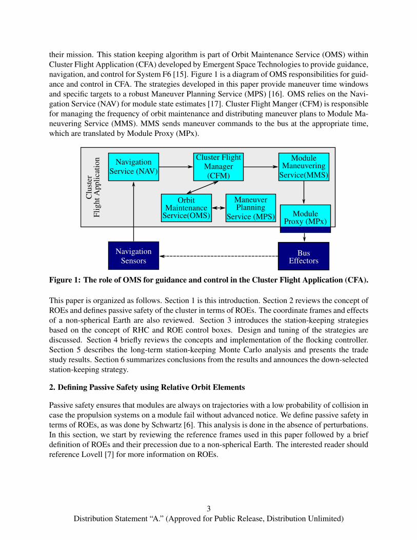
their mission. This station keeping algorithm is part of Orbit Maintenance Service (OMS) withinCluster Flight Application (CFA) developed by Emergent Space Technologies to provide guidance,navigation, and control for System F6 [15]. Figure 1 is a diagram of OMS responsibilities for guid-ance and control in CFA. The strategies developed in this paper provide maneuver time windowsand specific targets to a robust Maneuver Planning Service (MPS) [16]. OMS relies on the Navi-gation Service (NAV) for module state estimates [17]. Cluster Flight Manger (CFM) is responsiblefor managing the frequency of orbit maintenance and distributing maneuver plans to Module Ma-neuvering Service (MMS). MMS sends maneuver commands to the bus at the appropriate time,which are translated by Module Proxy (MPx).
NavigationSensors
NavigationService (NAV)
Cluster FlightManager(CFM)
Clu
ster
Flig
htA
pplic
atio
n
BusEffectors
ModuleManeuvering
Service(MMS)
OrbitMaintenance
Service(OMS)
ManeuverPlanning
Service (MPS) ModuleProxy (MPx)
Figure 1: The role of OMS for guidance and control in the Cluster Flight Application (CFA).
This paper is organized as follows. Section 1 is this introduction. Section 2 reviews the concept ofROEs and defines passive safety of the cluster in terms of ROEs. The coordinate frames and effectsof a non-spherical Earth are also reviewed. Section 3 introduces the station-keeping strategiesbased on the concept of RHC and ROE control boxes. Design and tuning of the strategies arediscussed. Section 4 briefly reviews the concepts and implementation of the flocking controller.Section 5 describes the long-term station-keeping Monte Carlo analysis and presents the tradestudy results. Section 6 summarizes conclusions from the results and announces the down-selectedstation-keeping strategy.
2. Defining Passive Safety using Relative Orbit Elements
Passive safety ensures that modules are always on trajectories with a low probability of collision incase the propulsion systems on a module fail without advanced notice. We define passive safety interms of ROEs, as was done by Schwartz [6]. This analysis is done in the absence of perturbations.In this section, we start by reviewing the reference frames used in this paper followed by a briefdefinition of ROEs and their precession due to a non-spherical Earth. The interested reader shouldreference Lovell [7] for more information on ROEs.
3Distribution Statement “A.” (Approved for Public Release, Distribution Unlimited)
2.1. Frames of Reference
The International Celestial Reference Frame (ICRF) represents absolute positioning relative toEarth. ICRF uses a quasi-inertial coordinate frame centered at the Earth and a set of orthogonalCartesian unit vectors with the z axis pointing through the North Pole. A useful frame for definingthe relative motion of two spacecraft is the RSW frame.∗ RSW is an orthogonal reference frame,often referred to as Hill’s frame [18] for circular orbits, centered at the origin of one spacecraftand rotating as it moves around in its reference orbit. Figure 2 demonstrates the geometry of theRSW frame at a single instance in the reference orbit. The x axis (R component) of RSW is definedalong the instantaneous position vector in the direction of zenith, which is referred to as the radialaxis. The z axis (W component) points in the direction of the orbit angular momentum vector, andis referred to as the cross-track axis. The y axis (S component) completes the orthogonal, righthanded coordinate system, which is referred to as the along-track axis because it points along thedirection of motion for the orbit. A local vertical curvilinear (LVC) frame is similar to RSW, butthe axes curve along the shape reference orbit. The y axis curves along the direction of along-trackmotion, and the z axis curves along the direction of cross-track motion as demonstrated in Fig. 2.This improves the accuracy of relative orbit propagation for long along-track distances.
x
yz
z
y
x
RSWICRF
x
yz
z
y
x
LVCICRF
Figure 2: Diagrams of RSW and LVC with respect to ICRF centered at the Earth’s originat an instance in time. The reference orbit is the dotted ellipse. LVC is an RSW frame withcurvilinear along-track axis (y) and curvilinear cross-track axis (z).
2.2. Relative Orbit Elements
ROEs are a six-tuple (ae, xd , yd , β , zmax, γ) that represents the geometry of a relative orbit in theLVC frame of a reference orbit. The transformation of LVC position and velocity to ROEs is anonlinear transformation defined by the following functions:
ae = 2
√(xω
)2
+
(3x+2
yω
)2
,
∗For circular orbits, the along-track and in-track directions are always the same, so this coordinate frame is some-times called ‘RIC.’
4Distribution Statement “A.” (Approved for Public Release, Distribution Unlimited)
xd = 4x+2yω,
yd = y−2xω,
β = arctan(
x3ωx+2y
),
zmax =
√(zω
)2
+ z2,
γ = arctan(
ωzz
)− arctan
(x
3ωx+2y
)(1)
where x, y, and z are the velocities in the radial, along-track, and cross-track directions, respec-tively. The inverse transformation also has a functional representation:
x = xd−ae
2sin(β ),
y = ae sin(β )+ yd,
z = zmax sin(γ +β ),
x =ae
2ω sin(β ),
y = aeω cos(β )− 32
ωxd,
z = zmaxω cos(γ +β )
The geometric interpretation of ROEs is the key to their usefulness. Figure 3 and later in Fig. 4diagram the geometric meaning of ROEs in LVC.
y
x
yd ae
β
(a) When xd = 0 the relative orbit is a closed andrepeating in the x-y plane.
y
x
xd
(b) When xd 6= 0 the relative orbit is open and drifts alongthe y axis (along-track).
Figure 3: Relative orbits in the x-y plane of the LVC frame when propagated using CWequations. These diagrams depict the effect of non-zero xd on the relative orbits. The ae, ydand β elements are also depicted.
5Distribution Statement “A.” (Approved for Public Release, Distribution Unlimited)
ROEs also simplify the propagation of relative orbits in the LVC, which is analogous to the simpli-fication that KOEs afford in the ICRF. The propagation of the ROEs is similar to the propagation ofposition and velocity using the Clohessy-Wiltshire (CW) equations on linearized relative motion[3]. Under Clohessy and Wiltshire’s assumption of a circular reference orbit, ae, xd , zmax and γ
remain constant. β (t) is propagated from β (0) using Eq. 2:
β (t) = β (0)+ωt (2)
where ω is the mean motion of the circular reference orbit. Hence, β is the phase angle of therelative orbit that results in the periodic angular motion. yd(t) is propagated from yd(0) using Eq.3:
yd(t) = yd(0)−32
ωxdt. (3)
If xd = 0, then there is no yd drift, and the relative orbit is closed as seen in Fig. 3a. When theenergy of the two absolute orbits is not equal, xd 6= 0, and secular drift in yd results as modeled inEq. 3 and shown in Fig. 3b. The difficulty of maintaining two orbits with exact xd = 0 motivatesthe concept of passive safety.
2.3. Definition of Passive Safety
It is extremely difficult (if not impossible) to equate the energies of two orbits when there is naviga-tion and thruster noise in the systems. Therefore, two orbits will almost certainly have a non-zeroxd with secular drift of yd . If the guidance, navigation, and control malfunctions, then the yd driftwill not be corrected at all. Therefore, the cluster of modules should maintain a passively safe con-figuration that prevents collisions when yd is not controlled. Because the yd drift is solely alongthe y-axis, this requirement equates to maintaining separation in the x-z plane.
Figure 4 is the geometric interpretation of ae, β , zmax, and γ in the x-z plane. Passive safety isdefined using the minimum separation of two relative orbits in the x-z plane of LVC. If the LVCframe is centered on one of the orbits, then it is defined as the minimum distance of ROEs from theorigin. The sub-figures of Fig. 4 demonstrate the effect of different γ values on the geometry ofrelative orbits in the x-z plane. As γ approaches 90° or 270°, the relative orbit will “tip over” itselfin the x-z plan and violate the rule of passive safety. Therefore, two orbits must meet the followingconditions in order to remain passively safe: ae
2 � r1 + r2 and zmax sin(γ)� r1 + r2 where r1 andr2 are the radii of the modules in the two orbits. These values should be significantly larger thanr1+ r2 to provide a reasonable guarantee of passive safety. For an in-depth discussion of passivelysafe cluster design, the interested reader can reference Schmidt [19].
2.4. Secular Drift Due to J2
Secular drift needs to be corrected periodically by station keeping in order to maintain the maxi-mum inter-module distance (IMD) of the cluster. As long as xd is non-zero, the corresponding ydsecular drift is much larger than the drift due to discarded nonlinear terms and higher order gravityterms due to non-spherical Earth. After non-zero xd , the second zonal harmonic of gravitationalforces due to non-spherical Earth (J2) is the largest contributor to relative drift of two orbits. J2causes significant secular drift of zmax and ae, which must be corrected over time to maintain the
6Distribution Statement “A.” (Approved for Public Release, Distribution Unlimited)
z
x
zmaxae2
(a) γ= 0° or γ= 180°
z
x zmax
ae2
r1
r2
(b) γ= 45°, γ= 135°, γ= 225° orγ= 315°
z
x zmax
ae2
(c) γ= 90° or γ= 270°
Figure 4: Relative orbits in the x-z plane of the LVC frame when propagated using CWequations. These diagrams depict the effects of ae, zmax and γ on the cluster. As γ approaches90° or 270°, the relative orbit is said to “tip over” on itself. The orbit is passively safe withrespect to the origin when ae > 0, zmax > 0, γ 6= 90° and γ 6= 270°.
cluster. J2 also causes drift of γ that threatens passive safety of the cluster. Research into J2-invariant relative orbits has shown that two orbits on the same inclination do not have any seculardrift in zmax or ae [5, 2]. Therefore, the strategies discussed in this paper place a high priority onmaintaining zero differential inclination. However, two orbits on the same inclination will stillexhibit drift in γ , which needs to be corrected periodically.
3. Loop Closure of Maneuver Planning for Station-Keeping
All of the station-keeping strategies developed in this paper utilize a common algorithm for loopclosure of maneuver planning. There are decision points in the algorithm that define the behavior ofdifferent strategies. Each strategy is defined by its method for deciding whether or not to generatenew maneuver plans and its method for determining the target timing that it uses to plan maneuvers.These methods and the tuning parameters of the strategies are presented below, including a detaileddiscussion of using ROEs to define control boxes and to determine maneuver targets.
3.1. Pseudo-Algorithm for Loop Closure of Maneuver Planning
The algorithm for loop closure of maneuver planning (LCMP) originates from the concept ofreceding horizon control (RHC). In its most basic form, LCMP is equivalent to RHC, but the moreeffective strategies deviate from true RHC to achieve desired performance characteristics.
The RHC problem is an optimal control problem solved repeatedly for a finite time window. Astime progresses, each repetition of RHC has the same amount of finite time for the optimal controlwindow. The significance of this is that the final time of the window is receding into the horizon.LCMP targets and maintains a desired relative orbit defined by a set of ROE, using state feedbackfrom the navigation system to update maneuver plans in the same manner as RHC. The algorithmis implemented as a cyclic process as shown in Fig. 5. Each iteration of the algorithm is a controlcycle. At the start of each cycle, the latest available state estimates from Navigation are used to
7Distribution Statement “A.” (Approved for Public Release, Distribution Unlimited)
NavigationUpdate
Start StationKeeping
ObjectivesSatisfied?
Wait for NextControl Cycle
yes
no DetermineManeuverWindow
Compute aNew Set ofManeuvers
Figure 5: Flow diagram for the LCMP algorithm. Different strategies have different controlobjects and different methods for determining the maneuver window.
predict if the module’s current set of maneuvers achieves the control objectives of the strategy foreach module in the cluster.
For most of the strategies, the objective is defined as a control box that is defined by ranges ofROEs. To improve performance, the strategies are implemented using a leader-follower controlarchitecture. At every check of the objectives, a leader is chosen for the cluster. Changing theleader frequently balances the fuel requirements across the cluster, but changing the leader toofrequently can cause excessive trajectory corrections. The control box ROE ranges are computedand checked with respect to the current leader. If the objectives are not satisfied, then OMS requestsa new set of maneuvers from Maneuver Planning Service (MPS) as shown in Fig. 1.
The request includes a list of modules that need new maneuver plans, a desired target (or targetrange), and a maneuver window for achieving that target. The decision process for determining thetarget and maneuver window is unique to each strategy. The algorithm used for optimal maneuverplanning, which uses the Gim-Alfriend state transition matrix with linearized eccentricity and J2to solve the maneuver planning problem [20], and its implementation are detailed by Brown [16].The algorithm computes a maneuver plan that achieves the target with minimal fuel consumptionmodeled as the total ∆V of all the maneuvers in the plan. After maneuver planning is complete,the algorithm pauses until the next control cycle.
3.2. Strategies for Control Objectives and Maneuver Windows
The primary inspiration for LCMP is Tillerson [4], who solves convex programs to achieve ∆Voptimal maneuvers. For station-keeping, Tillerson uses an inner and outer control box. When therelative trajectory violates the outer control box, a ∆V optimal maneuver plan is solved that returnsthe module to the inner control box. LCMP can be configured similarly but offers more variety inits selection of maneuver windows and control objectives.
Figures 6 through 8 demonstrate the three different strategies for evaluating control objectives anddetermining maneuver windows. If the system does not have a strict convergence deadline, thenthe first strategy configures LCMP to use a receding horizon that conserves energy. Instead ofevaluating control objectives, RHC requests a maneuver plan every control cycle as demonstratedin Fig. 6. Every control cycle uses the same maneuver window size, which causes the target
8Distribution Statement “A.” (Approved for Public Release, Distribution Unlimited)
TimeControl cycle 1st replan 2nd replan Target time of 1st
1st maneuver window Subsequent maneuver windows
maneuver windowFigure 6: Manuever windows for RHC. A new maneuver plan is created at every step of thecontrol cycle, and the maneuver window recedes into the horizon over time.
TimeControl Cycle
Predict noviolation & replan
Target time of 1st
1st maneuver window Subsequent maneuver window
maneuver windowControl box
violations
Figure 7: Maneuver windows for pRHwCB. At every step of the control cycle, the module’slatest state estimate and current maneuver plan are checked against its control box. If thecontrol box is satisfied, then the current maneuver plan is deemed acceptable.
TimeControl Cycle
Predict noviolation & replan
Target time of 1st
1st maneuver window Subsequent maneuver window
maneuver windowControl box
violations
New manuever windowwhen violated again
Figure 8: Maneuver windows for FHwCB. If a control box is violated when there are nomaneuver plans for that module, then a full maneuver window is used. If the module has amaneuver plan, then the new window has the same target time as the current maneuver plan.
time to recede into the horizon. This implements traditional RHC, and could be proven to haveguaranteed stability with a suitable maneuver planning subsystem by applying the methods inMayne [13].
The second strategy is a modification to traditional RHC with the addition of control boxes. Figure7 demonstrates LCMP with control boxes, which is named pseudo-receding horizon with controlboxes (pRHwCB). If the current maneuver plan ends within the control box, then pRHwCB doesnot request a new maneuver plan. This approach has less frequent maneuvers when the minimumimpulse requirement is large. pRHwCB can be configured with inner and outer control boxes likein Tillerson [4], but a single control box was found to be more effective. In an attempt to furtherreduce the maneuver frequency, fixed horizon control with control boxes (FHwCB) is introducedas the third strategy. FHwCB fixes the target time of subsequent maneuver plan windows to thetarget time of the first maneuver window. This essentially shrinks the size of the maneuver windowof subsequent maneuver plans, which is demonstrated in Fig. 8. The computation of target ROEswithin the control boxes for pRHwCB and FHwCB are discussed in the next section.
9Distribution Statement “A.” (Approved for Public Release, Distribution Unlimited)
zmax error
ae error
navigation noise
osculating effectstargeting errors
Drifting satelliteControl box
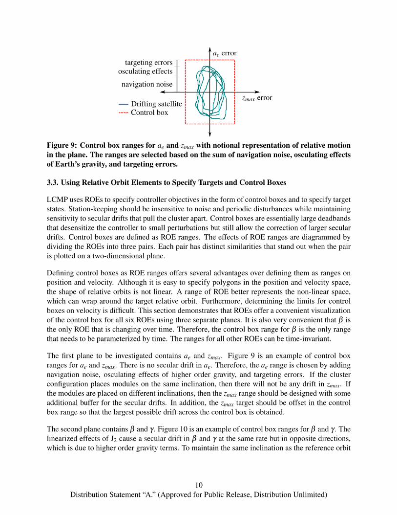
Figure 9: Control box ranges for ae and zmax with notional representation of relative motionin the plane. The ranges are selected based on the sum of navigation noise, osculating effectsof Earth’s gravity, and targeting errors.
3.3. Using Relative Orbit Elements to Specify Targets and Control Boxes
LCMP uses ROEs to specify controller objectives in the form of control boxes and to specify targetstates. Station-keeping should be insensitive to noise and periodic disturbances while maintainingsensitivity to secular drifts that pull the cluster apart. Control boxes are essentially large deadbandsthat desensitize the controller to small perturbations but still allow the correction of larger seculardrifts. Control boxes are defined as ROE ranges. The effects of ROE ranges are diagrammed bydividing the ROEs into three pairs. Each pair has distinct similarities that stand out when the pairis plotted on a two-dimensional plane.
Defining control boxes as ROE ranges offers several advantages over defining them as ranges onposition and velocity. Although it is easy to specify polygons in the position and velocity space,the shape of relative orbits is not linear. A range of ROE better represents the non-linear space,which can wrap around the target relative orbit. Furthermore, determining the limits for controlboxes on velocity is difficult. This section demonstrates that ROEs offer a convenient visualizationof the control box for all six ROEs using three separate planes. It is also very convenient that β isthe only ROE that is changing over time. Therefore, the control box range for β is the only rangethat needs to be parameterized by time. The ranges for all other ROEs can be time-invariant.
The first plane to be investigated contains ae and zmax. Figure 9 is an example of control boxranges for ae and zmax. There is no secular drift in ae. Therefore, the ae range is chosen by addingnavigation noise, osculating effects of higher order gravity, and targeting errors. If the clusterconfiguration places modules on the same inclination, then there will not be any drift in zmax. Ifthe modules are placed on different inclinations, then the zmax range should be designed with someadditional buffer for the secular drifts. In addition, the zmax target should be offset in the controlbox range so that the largest possible drift across the control box is obtained.
The second plane contains β and γ . Figure 10 is an example of control box ranges for β and γ . Thelinearized effects of J2 cause a secular drift in β and γ at the same rate but in opposite directions,which is due to higher order gravity terms. To maintain the same inclination as the reference orbit
10Distribution Statement “A.” (Approved for Public Release, Distribution Unlimited)
β error
γ error
navigation noiseosculating effects
targeting errors
Drifting β
Maneuver plan to correct β
largest passively
Control box without inclination limitControl box with inclination limit
safe drift in β
Figure 10: Control box ranges for β and γ with a notional representation of relative motionin the plane. The ranges are coupled because β and γ have a secular drift at the same rate.
the relationshipβ + γ = θre f (4)
must be maintained on average where θre f is the true argument of longitude of the reference orbit.The natural drift of β (the Drifting β arrow in Fig. 10) maintains this relationship. To preventfrequent burns, β is allowed to drift as far as possible, without violating passive safety. If γ wereallowed an equal range, then Eq. 4 would be violated significantly at the far corners (dotted line inFig. 10). Therefore, the control box around β and γ is designed as a parallelogram.
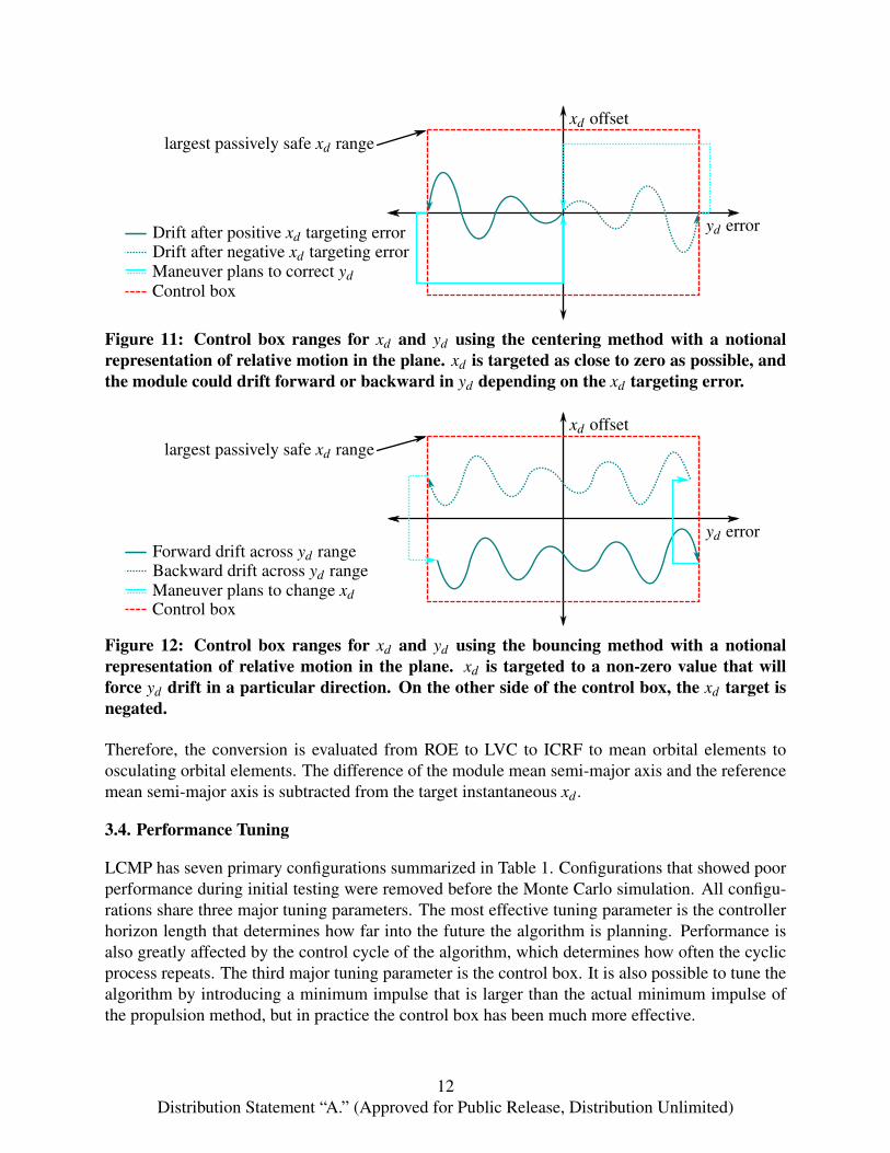
The third plane contains xd and yd , which sees the most secular drift when xd 6= 0. Two differentmethods can be used to control motion along this plane. The first method is the centering method,which Fig. 11 demonstrates. Natural motion causes the module to drift to the limits of yd . Whenthe limit is reached, the module is targeted back to the center of the control box for yd and to xd = 0.Because navigation and guidance is not perfect, xd = 0 will not be obtained exactly, and the processwill continue. The second method is the bouncing method, which Fig. 12 demonstrates. Instead oftargeting back to the center of the yd range and xd = 0, this method purposely sets an xd offset thatis large enough to guarantee that yd will drift in a certain direction. This method is more efficientfor large yd ranges.
3.3.1. Maintenance of Equal Energy
The centering method and bouncing method for xd and yd control rely on accurate targeting of xd .The target specified for xd is the desired semi-major axis difference of the target relative orbit withrespect to the reference orbit. Unfortunately, higher order gravity terms cause periodic oscillationsin the instantaneous semi-major axis of the module and reference. Therefore, the xd target shouldbe the mean semi-major axis difference. Therefore, LCMP adjusts the instantaneous xd target sothat the mean semi-major axis difference is correct.
The xd adjustment is accomplished by using an osculating to mean orbital element conversion [21].To avoid the numerical inaccuracies that accumulate from transforming from ROE to LVC to ICRFto mean orbital elements to osculating orbital elements, and then back to ICRF, LVC and ROE, ashortcut is used that only adjust the xd ROE. xd is defined as the difference in semi-major axes.
11Distribution Statement “A.” (Approved for Public Release, Distribution Unlimited)
yd error
xd offset
Drift after positive xd targeting errorDrift after negative xd targeting errorManeuver plans to correct ydControl box
largest passively safe xd range
Figure 11: Control box ranges for xd and yd using the centering method with a notionalrepresentation of relative motion in the plane. xd is targeted as close to zero as possible, andthe module could drift forward or backward in yd depending on the xd targeting error.
yd error
xd offset
Forward drift across yd rangeBackward drift across yd rangeManeuver plans to change xd
largest passively safe xd range
Control box
Figure 12: Control box ranges for xd and yd using the bouncing method with a notionalrepresentation of relative motion in the plane. xd is targeted to a non-zero value that willforce yd drift in a particular direction. On the other side of the control box, the xd target isnegated.
Therefore, the conversion is evaluated from ROE to LVC to ICRF to mean orbital elements toosculating orbital elements. The difference of the module mean semi-major axis and the referencemean semi-major axis is subtracted from the target instantaneous xd .
3.4. Performance Tuning
LCMP has seven primary configurations summarized in Table 1. Configurations that showed poorperformance during initial testing were removed before the Monte Carlo simulation. All configu-rations share three major tuning parameters. The most effective tuning parameter is the controllerhorizon length that determines how far into the future the algorithm is planning. Performance isalso greatly affected by the control cycle of the algorithm, which determines how often the cyclicprocess repeats. The third major tuning parameter is the control box. It is also possible to tune thealgorithm by introducing a minimum impulse that is larger than the actual minimum impulse ofthe propulsion method, but in practice the control box has been much more effective.
12Distribution Statement “A.” (Approved for Public Release, Distribution Unlimited)
Table 1: Summary of several strategies configured for station-keeping using LCMP.
Strategy ControlObjective
ManeuverWindow
ControlBoxes
TargetingMethod
Monte CarloPerformed
RHC Always plan Receding NoneDirect
targeting !
pRHwCBCentering
ROE controlbox
Receding Outer onlyCenter of
control box !
pRHwCBBouncing
ROE controlbox
Receding Outer onlyBouncing
insidecontrol box
!
pRHwCBCentering
Inner/Outer
ROE controlbox
RecedingInner and
OuterCenter of
control box
FHwCBCentering
ROE controlbox
Shrinking Outer onlyCenter of
control box !
FHwCBBouncing
ROE controlbox
Shrinking Outer onlyBouncing
insidecontrol box
FHwCBCentering
Inner/Outer
ROE controlbox
ShrinkingInner and
outerCenter of
control box
The control horizon is the most effective parameter for tuning the controller. A shorter horizoncauses more frequent burns and larger total ∆V , but reduces trajectory dispersions. A longer hori-zon will slightly reduce burn frequency, but it will also increase trajectory dispersions. See Fig.13 for a four module example with a short horizon of 6 control cycle periods and Fig. 14 for anexample with a long horizon of 12 control cycle periods. The control period is 1450 seconds, thethruster is 10 N and the control box is disabled. The results were obtained by simulating over 300orbits with perfect navigation, and the ∆V results are extrapolated for a six month mission.
Reducing the control cycle period of LCMP increases the ∆V . When LCMP checks maneuverplans too often, the targeting errors introduced by unmodeled dynamics and navigation noise willcause repeated planning and extra burns. A large control box can help to alleviate this problem,but it is not a cure. One should exercise caution when increasing the control cycle, because anincreased control cycle can result in larger trajectory dispersions and even instability.
Tuning the control box is the least effective method for reducing ∆V . However, it is absolutelycritical for reducing burn frequency. A larger control box allows the modules to drift furtherbefore maneuvers are scheduled to return the module to its original position, which decreases burnfrequency but results in much larger trajectory dispersions. Figure 15 provides an example with alarge control box. The total ∆V over six months is larger than the previous example with the samehorizon length of 12 control cycle periods, but burns occur less frequently at 11.4 orbits betweenburns instead of 6.6 orbits between burns without a control box.
13Distribution Statement “A.” (Approved for Public Release, Distribution Unlimited)
x=
r-bar
(m)
z=crosstrack (m)y=v-bar (m)−1000
0
1000
2000
−4000
400
−400
−200
0
200
400
(a) Module trajectories in the LVC frame of the first module thatdemonstrate small trajectory dispersions. There are 2.8 orbits be-tween burns.
Est
imate
ddelt
a-V
(m/s
)
Module Numbers
1 2 3 40
2
4
6
(b) Estimated total ∆V over sixmonths for the cluster is 19.2 m/s.
Figure 13: Station-keeping performance with control box disabled and a short horizon of 6control cycle periods.
x=
r-bar
(m)
z=crosstrack (m)
y=v-bar (m)−1000
0
1000
2000
−4000
400
−400
−200
0
200
400
(a) Module trajectories in the LVC frame of the first module thatdemonstrate medium trajectory dispersions. There are 6.6 orbitsbetween burns.
Est
imate
ddelt
a-V
(m/s
)
Module Numbers
1 2 3 40
2
4
6
(b) Estimated total ∆V over sixmonths for the cluster is 8.59 m/s.
Figure 14: Station-keeping performance with control box disabled and a long horizon of 12control cycle periods.
4. Review of the Flocking Controller for Station-Keeping
The flocking controller was first developed by Schwartz and Krenzke [6]. It is designed aroundthe idea that a cluster of modules does not need to hold a formation in order to stay together.Instead of formation keeping, this controller aims only to keep the cluster together and maintainthe modules in passively safe orbits while minimizing fuel use and burn frequency. Passive safetyis parameterized by a safe zone size that is a distance to maintain separation in the x-z plane ofLVC. Control of in-plane motion is performed by a proportional derivative (PD) controller with adeadband.
14Distribution Statement “A.” (Approved for Public Release, Distribution Unlimited)
x=
r-bar
(m)
z=crosstrack (m)
y=v-bar (m)−2000−1000
01000
20003000
4000
−4000
400
−500
0
500
(a) Module trajectories in the LVC frame of the first module thatdemonstrate large trajectory dispersions. There are 11.4 orbits betweenburns.
Est
imate
ddelt
a-V
(m/s
)
Module Numbers
1 2 3 40
2
4
6
(b) Estimated total ∆V over sixmonths for the cluster is 13.7 m/s.
Figure 15: Station-keeping performance with a control box that allows relative large along-track drift and horizon of 12 control cycle periods.
The flocking controller will act to enforce a safety zone. The safety zone size determines the prob-ability of collision and minimum safe distance permitted by the controller. However, a larger safetyzone translates into a larger danger zone that requires larger burns for a module to transfer acrossthe danger zone. To establish the safety zone, the flocking controller maintains three conditionsbetween each pair of module ROEs. First, each pair’s zmax must be above a minimum boundary,which is set by the safety zone size. Second, each pair’s ae must be above a minimum boundary,which is set by the safety zone size. Third, each pair’s γ must not be approaching 90° or 270°.More precisely, each neighbor’s gamma value must be a certain angular distance away from 90°and 270°, and this angular distance is computed from the zone size and the pair’s current zmaxand ae. Corrections of γ are made using a maneuver that is fired along the y axis, ∆Vy, which iscomputed from a relationship derived from Eq. 1:
∆γ = arctan(
ωzmax sin(γ +β +ωtb)ωzmax0 cos(γ +β +ωtb)
)− arctan
(ae sin(β +ωtb)
ae cos(β +ωtb)+ 4ω
∆Vy
)where tb is the time of the burn. The time of the maneuver is limited to perigee or apogee tominimize the size of the required ∆V .
Corrections for along-track drift follow a PD control scheme. The controller observes the currentyd and yd drift rate with respect to the leader module. Then, using a set of PD gains, it performsa burn that biases xd to correct the situation. The PD controller includes limits on yd and xd ,which are also used as tuning parameters. The yd limit is essentially a proportional saturation limitbecause it represents the maximum yd offset that will be used in the controller computation. The xdlimit is essentially a deadband. It represents the minimum value of xd correction that will trigger amaneuver.
The PD burns and the γ correction burns not only affect the intended ROEs, but also all otherROEs. Therefore, the PD controller verifies that a maneuver will not violate the safety zone of any
15Distribution Statement “A.” (Approved for Public Release, Distribution Unlimited)
pair before the maneuver is scheduled. The PD controller and γ correction also adhere to upperbounds on ae and zmax. Neither will schedule burns that violate these upper bounds.
5. Performance Analysis and Station-Keeping Results
Station-keeping performance is critical to guaranteeing the mission lifetime. The cluster will beperforming station-keeping maneuvers for the majority of the mission, and fuel is a limited re-source. If the station-keeping performance does not meet expectations, then the mission lifetimewill be reduced accordingly. This section summarizes the key performance measures and perfor-mance tuning of LCMP. The differences between RHC, pRHwCB, FHwCB, and flocking controllerare also discussed.
5.1. Mission Scenario
Station-keeping performance of a four module cluster is analyzed for a sun synchronous orbit. Theparameters of the orbit are summarized in Table 2. Table 3 is the cluster configuration that wasused for evaluation, which is plotted for a few orbits in Fig. 16. Each module has a GPS receiver,and they are using GPS filters for navigation as described by Schmidt [17]. The GPS filters aretracking the same GPS satellites to reduce relative navigation errors. The true gravity model is a12x12 model. There is an exponential drag model that is inconsequential at an altitude of 500 km.The true thruster model is an RCS model with a short rise time and fall time. The thruster provides70 N of force with a specific impulse (ISP) of 230 seconds. The minimum impulse provided bythis thruster is 1.3 cm/sec. Although the simulation does not model attitude control, noisy burndirections are modeled. Thruster direction noise is a Gaussian distributed white noise in azimuthangle and elevation angle of the burn. The three-sigma value of the noise for each angle is sixdegrees, which is modeled from 2 degrees of sensor error plus 1 degree of deadband plus 3 degreesof alignment error. Guidance and control is using a J2 gravity model in its computations.
Table 2: Orbital parameters for station-keeping evaluationParameter Value
altitude 500 kminclination 98.2°eccentricity 0
right ascension of the ascending node 0°argument of perigee 0°true anomaly at start 0°
time at start (sec after J2000) 134308851.184
Monte Carlo simulation was used to validate performance of the station-keeping method. Fortyruns of 500 orbits were conducted for each configuration of the controllers. During every run, eachmodule is the leader for 125 contiguous orbits to balance fuel. Each run uses a different streamof random numbers, which affects the navigation noise and thruster noise. In addition, the initialpositions of the modules are randomized within the β -γ and xd control boxes. Initial conditionsfor β and γ are still chosen so that modules start out on the same inclination.
16Distribution Statement “A.” (Approved for Public Release, Distribution Unlimited)
Table 3: Initial cluster configuration and ROE targets with four modules used to evaluateperformance.
Module 1 Module 2 Module 3 Module 4ae 378 m 378 m 1073 m 1073 mxd 0 m 0 m 0 m 0 myd 0 m 0 m 0 m 0 mβ 270° 90° 270° 90°
zmax 179 m 179 m 537 m 537 mγ 0° 0° 0° 0°
Module 4
Module 3
Module 2
Module 1
Module 4
Module 3
Module 2
Module 1
x=
r-bar
(m)
z=crosstrack (m)y=v-bar (m)−500
0
500
−2000
200
−200
0
200
Figure 16: Initial cluster configuration for station-keeping simulation, which is plotted inLVC for one orbit starting at the modules initial conditions.
5.2. Performance Measures
The primary performance measure for station-keeping is total ∆V for station-keeping during themission, which reflects the amount of fuel required. The following is a list of other performancemeasures, which usually conflict with minimizing ∆V :
Burn Frequency Infrequent maneuvering is desirable to provide more opportunity for scientificstudies, which may be interrupted while the module is slewing and accelerating.
Burn Angles The angles of burns are important when the mission requires the module to point ata specific attitude.
Inter-module Distances The minimum IMD and maximum IMD specified for the cluster shouldnot be violated. In practice, noise and disturbances will cause violations of the minimumIMD. Therefore, significant violations of IMD were noted.
Stability and Trajectories The mission may require accurate tracking of the cluster configura-tion. In this case, minimizing dispersions from the nominal trajectory often requires morefrequent burns that increase total ∆V over the module lifetime.
Thruster Size Although minimal station-keeping ∆V is more easily achieved using small, fre-quent burns, the F6 cluster required large thrusters to meet the requirements of a scattermaneuver during the mission. A large 70N thruster was used for these studies, which is a
17Distribution Statement “A.” (Approved for Public Release, Distribution Unlimited)
thruster that is capable of achieving the scatter requirement [22].
5.3. Monte Carlo Simulation Results
Table 4 details the results of Monte Carlo simulation conducted for the study. CC is the controlcycle in orbits, which is 0.5 orbit if not specified. MW is the maneuver window length in orbits.For example, RHC CC3 MW9 has a control cycle of three orbits and a maneuver window of nineorbits. pRHwCB Centering, 4km yd , MW3 is using the centering method for yd control with a 4km range across the yd control box and a control cycle of three orbits.
The 500 orbit ∆V number was extrapolated to estimate the ∆V for a six month mission. The three-sigma (3σ ) value of the ∆V for six months over thirty runs is also listed. The ratio of the smallestsix month ∆V to the largest six month ∆V also provides some indication of the variance in perfor-mance. Frequency of maneuvers is quantified by the average orbits between burns. Minimum andmaximum IMD are sampled every 10 seconds, and the extreme values over 30 runs are tabulated.IMD in the x-z plane is sampled every 60 seconds. Figure 17 and Fig. 18 visualize the ∆V con-sumption and the burn frequency results of the simulations, respectively. Probability of collisionwas computed using the covariance computed within the navigation filters, and it was zero for allcases.
Table 4: Detailed results of Monte Carlo simulation for station-keeping strategies.
RHC MW3 has acceptable ∆V performance over six months, but the burn frequency is very highat about one burn for every nine orbits. A wide range of tunings were attempted in order toreduce the burn frequency without increasing the six month ∆V . The RHC CC3 MW3 tuning has
18Distribution Statement “A.” (Approved for Public Release, Distribution Unlimited)
∆V
(m/s
)
RHCMW3
RHCCC3
MW9
pRHwCB
Centering
MW3
pRHwCB
Centering
MW2
pRHwCB
Bouncing
MW2
FHwCBCentering
MW3
Flocking
Controller
0
2
4
6
8
10
12
Figure 17: Graphical ∆V summary for the station-keeping methods in Table 4.
Per
iod
Bet
wee
nM
aneu
ver
s(s
ec)
RHCMW3
RHCCC3
MW9
pRHwCB
Centering
MW3
pRHwCB
Centering
MW2
pRHwCB
Bouncing
MW2
FHwCBCentering
MW3
Flocking
Controller
0
5
10
15
20
25
30
Figure 18: Graphical burn frequency summary for the station-keeping methods in Table 4.
a much lower burn frequency of one burn for every nineteen orbits, however, checking the orbitsinfrequently at a control cycle of three orbits can lead to stability issues. Although this tuningmaintains a safe minimum IMD, the higher maximum IMD indicates that the dispersions from thetarget orbits are much larger than with RHC MW3. Therefore, in spite of the favorable numbersfor the other performance measures, RHC CC3 MW3 is not recommended.
The control box approaches are the most stable, and they also have hard limits on the module po-sitions during drift periods. Both pRHwCB and FHwCB maintain the cluster using small total ∆Vand infrequent maneuvers. The only tuning of pRHwCB that had poor performance was Center-ing with MW2 where the short maneuver window of two orbits causes dangerous flybys when themodules return to the center of the xd-yd control box. The modules use extra fuel to avoid theseflybys at the last minute, which is reflected in the total ∆V .
The results indicate that the flocking controller is least efficient, but the data in Table 4 does not
19Distribution Statement “A.” (Approved for Public Release, Distribution Unlimited)
tell the entire story. For most runs, the flocking controller was efficient as indicated by the lowerlimit of the ∆V range, but it occasionally encountered problems finding efficient changes for γ .These few cases skew the results dramatically. In addition, flocking controller lacks differentialinclination control. The effects of non-zero differential inclination build up over a 500 orbit simu-lation.
6. Conclusions
Ultimately, selection of a station-keeping strategy depends on the mission objectives and modulecapabilities such as mission-specific quiet periods, a required mission formation, or the minimumimpulse of the thruster. Table 5 is a summary of advantages and disadvantages for each algorithm.A flexible strategy that is configurable for RHC, pRHwCB, and FHwCB is implemented in OMS aspart of CFA. The centering and bouncing methods are also configurable. pRHwCB with centeringis the most efficient station-keeping for the simulated mission, and it is the method that is currentlybeing validated for long runs of CFA using a software in the loop simulation.
Table 5: Summary of advantages for the investigated station-keeping strategies.Algorithm Advantages Disadvantages
RHC Consistent burn directionsFrequent replanning; Potential for highburn frequency; No guaranteed finite
convergence time
pRHwCBOnly replans when necessary; Lowerburn frequency than RHC; Flexible
design (encompasses RHC)
Unpredictable maneuver windows;Less consistent burn directions; Noguaranteed finite convergence time
Flocking Low burn frequencyNo ae, zmax, inclination control, or
formation keeping; Single burnmaneuvers
The flocking concept could be a viable control strategy worth further R&D study, but the currentimplementation does not demonstrate enough performance improvement over the pRHwCB towarrant its use. A ‘hybrid’ controller was attempted that combines the pRHwCB method withrules of Flocking to determine γ . Testing of this controller in long simulations revealed severaldefects in the algorithms that have not been addressed. However, in theory a set of flocking rulesshould exist that would, at the very least, replicate the functionality of pRHwCB by considering thelong-term effects of a chosen target γ . Such rules may also be able to take advantage of situationsthat allow for more γ drift than passively safe control boxes would allow.
7. Acknowledgement
The authors would like to thank Allen Brown and Eric Ferguson for the assistance that they pro-vided while incorporating MPS into the simulation environment. The authors would also liketo thank Liam Healy and the System F6 team for their recommendations that guided this re-search.
20Distribution Statement “A.” (Approved for Public Release, Distribution Unlimited)
Distribution Statement “A.” (Approved for Public Release, Distribution Unlimited)
The views expressed are those of the author and do not reflect the official policy or position of theDepartment of Defense or the U.S. Government.
8. References
[1] Brown, O., Long, A., Shah, N., and Eremenko, P. “System Lifecycle Cost Under Uncertaintyas a Design Metric Encompassing the Value of Architectural Flexibility.” AIAA SPACE 2007 Con-ference & Exposition. Long Beach, CA, September 2007.
[2] Schaub, H. and Alfriend, K. T. “J2-Invariant Relative Orbits for Spacecraft Formations.” Ce-lestial Mechanics and Dynamical Astronomy, Vol. 79, No. 2, 2001, pp. 77–95.
[3] Clohessy, W. H. and Wiltshire, R. S. “Terminal Guidance System for Satellite Rendezvous.”Journal of the Aerospace Sciences, Vol. 27, No. 9, 1960, pp. 653–658.
[4] Tillerson, M., Inalhan, G., and How, J. “Co-ordination and Control of Distributed SpacecraftSystems Using Convex Optimization Techniques.” International Journal of Robust and NonlinearControl, Vol. 12, No. 2-3, 2002, pp. 207–242.
[5] Vadali, S. R., Sengupta, P., Yan, H., and Alfriend, K. T. “Fundamental Frequencies of Satel-lite Relative Motion and Control of Formations.” Journal of Guidance, Control, and Dynamics,Vol. 31, No. 5, September–October 2008, pp. 1239–1248.
[6] Schwartz, J. and Krenzke, T. “The Flocking Controller: A Novel Cluster Control Strategyfor Space Vehicles.” AIAA Guidance, Navigation, and Control Conference. No. AIAA-2013-4543,Boston, MA, August 2013.
[7] Lovell, T. A. and Tragesser, S. G. “Guidance for Relative Motion of Low Earth Orbit Space-craft Based on Relative Orbit Elements.” AIAA/AAS Astrodynamics Specialist Conference and Ex-hibit. Providence, RI, August 2004.
[8] Schwartz, J. and Krenzke, T. “Error-Contracting Impulse Controller for Satellite Cluster FlightFormation.” AIAA Guidance, Navigation, and Control Conference. No. AIAA-2013-4541, Boston,MA, August 2013.
[9] Breger, L. and How, J. P. “Gauss’s Variational Equation-Based Dynamics and Control forFormation Flying Spacecraft.” Journal of Guidance, Control, and Dynamics, Vol. 30, No. 2, 2007,pp. 437–448.
[10] Vadali, S. R., Yan, H. and Alfriend, K. T., “Formation Maintenance and Fuel Balancing forSatellites with Impulsive Control.” AIAA/AAS Aerodynamic Specialist Conference and Exhibit.Honalulu, HI, August 2008.
[11] Larsson, R., Berge, S. Bodin, P., and Jonsson, U., “Fuel Efficient Relative Orbit ControlStrategies for Formation Flying and Rendezvous within PRISMA.” Advances in the Astronautical
21Distribution Statement “A.” (Approved for Public Release, Distribution Unlimited)
Sciences, Vol. 125, 2006, pp. 25.
[12] Rawlings, J. “Tutorial Overview of Model Predictive Control.” IEEE Control Systems,Vol. 20, No. 3, 2000, pp. 38–52.
[13] Mayne, D., Rawlings, J., Rao, C., and Scokaert, P. “Constrained Model Predictive Control:Stability and Optimality.” Automatica, Vol. 36, No. 6, 2000, pp. 789–814.
[14] Saponara, M., Barrena, V., Bemporad, A., Hartley, E., Maciejowski, J., Richards, A., Tramu-tola, A., and Trodden, P. “Model Predictive Control Application to Spacecraft Rendezvous in MarsSample Return Scenario.” Progress in Flight Dynamics, Guidance, Navigation, Control, Fault De-tection, and Avionics, Vol. 6, December 2013, pp. 137–158.
[15] Hur-Diaz, S. and O’Connor, B. “Cluster Flight Application On System F6.” The 24th Inter-national Symposium on Space Flight Dynamics, Laurel, MD, May 2014.
[16] Brown, A., Ruschmann, M. C., Duffy, B., Ward, L. Hur-Diaz, S., Ferguson, E., and Stew-art, S. M., “Simulated Annealing Maneuver Planner for Cluster Flight.” The 24th InternationalSymposium on Space Flight Dynamics. Laurel, MD, May 2014.
[17] Schmidt, J. and Phillips, M. “A Distributed, Redundant Navigation and Fault Detection Sys-tem for DARPA System F6.” AIAA Guidance, Navigation, and Control Conference. No. AIAA-2013-4963, Boston, MA, August 2013.
[18] Hill, G., “Researches in the Lunar Theory.” American Journal of Mathematics, Vol. 1, No. 1,1878, pp. 5–26.
[19] Schmidt, J., Phillips, M., and Ruschmann, M. “Satellite Cluster Flight Design Considera-tions.” The 24th International Symposium on Space Flight Dynamics. Laurel, MD, May 2014.
[20] Gim, D.-W. and Alfriend, K. T. “State Transition Matrix of Relative Motion for the PerturbedNoncircular Reference Orbit.” Journal of Guidance, Control, and Dynamics, Vol. 26, No. 6, 2003,pp. 956–971.
[21] Cain, B. J. “Determination of Mean Elements for Brouwer’s Satellite Theory.” The Astro-nomical Journal, Vol. 67, No. 6, August 1962, pp. 391.
[22] Duffy, B., Brown, A., Ruschmann, M. C., Pinon III, E., and Ward, L. “Scatter Strategies forCluster Flight.” The 24th International Symposium on Space Flight Dynamics. Laurel, MD, May2014.
22Distribution Statement “A.” (Approved for Public Release, Distribution Unlimited)


![ASSESSMENT OF GNC IMPACTS OF CHEMICAL PLUME …issfd.org/ISSFD_2014/ISSFD24_Paper_S9-4_Carnelli.pdf · The Mango spacecraft is part of the PRISMA mission [5] and will be the chaser](https://static.documents.pub/doc/80x56/5cde567f88c9930b778ce5fd/assessment-of-gnc-impacts-of-chemical-plume-issfdorgissfd2014issfd24papers9-4.jpg)


