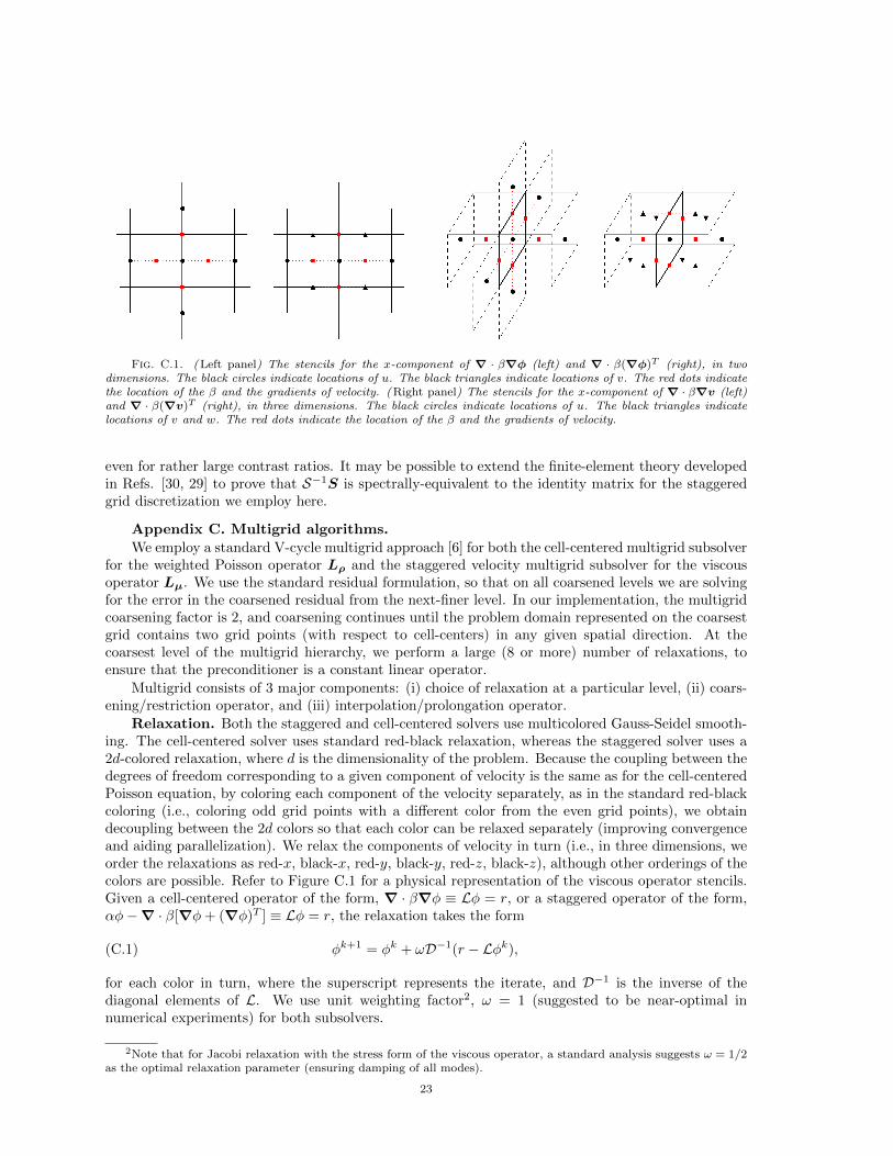
EFFICIENT VARIABLE-COEFFICIENT FINITE-VOLUME STOKES SOLVERS

MINGCHAO CAI ∗, ANDY NONAKA † , JOHN B. BELL ‡ , BOYCE E. GRIFFITH § , AND ALEKSANDAR

DONEV ¶

Abstract. We investigate several robust preconditioners for solving the saddle-point linear systems that arise fromspatial discretization of unsteady and steady variable-coefficient Stokes equations on a uniform staggered grid. Buildingon the success of using the classical projection method as a preconditioner for the coupled velocity-pressure system [B.E. Griffith, J. Comp. Phys., 228 (2009), pp. 7565–7595 ], as well as established techniques for steady and unsteadyStokes flow in the finite-element literature, we construct preconditioners that employ independent generalized Helmholtzand Poisson solvers for the velocity and pressure subproblems. We demonstrate that only a single cycle of a standardgeometric multigrid algorithm serves as an effective inexact solver for each of these subproblems. Contrary to traditionalwisdom, we find that the Stokes problem can be solved nearly as efficiently as the independent pressure and velocitysubproblems, making the overall cost of solving the Stokes system comparable to the cost of classical projection orfractional step methods for incompressible flow, even for steady flow and in the presence of large density and viscositycontrasts. Two of the five preconditioners considered here are found to be robust to GMRES restarts and to increasingproblem size, making them suitable for large-scale problems. Our work opens many possibilities for constructing novelunsplit temporal integrators for finite-volume spatial discretizations of the equations of low Mach and incompressibleflow dynamics.

Keywords Stokes flow; variable density; variable viscosity; saddle point problems; projectionmethod; preconditioning; GMRES.

1. Introduction. Many numerical methods for solving the time-dependent (unsteady) incom-pressible [3, 1, 27, 24] or low Mach number [43, 14] equations require the solution of a linear unsteadyStokes flow subproblem. The linear steady Stokes problem is of particular interest for low Reynoldsnumber flows [42, 26] or flow in viscous boundary layers. In this work, we investigate efficient linearsolvers for the unsteady and steady Stokes equations in the presence of variable density and viscosity.Specifically, we consider the coupled velocity-pressure Stokes system [49, 20]

ρut + ∇p = ∇ · τ (u) + f ,∇ · u = g,

(1.1)

where ρ (r) is the density, u (r, t) is the velocity, p (r, t) is the pressure, f (r, t) is a force density,and τ (u) is the viscous stress tensor. A nonzero velocity-divergence g (r, t) arises, for example, inlow Mach number models because of compositional or temperature variations [43]. The viscous stressτ (u) is µ∇u for constant viscosity incompressible flow, µ

[∇u+ (∇u)T

]when g = 0 (incompressible

flow), and µ[∇u+ (∇u)T

]+ (γ − 2

3µ)(∇ · u)I when g 6= 0, where µ (r, t) is the shear viscosityand γ (r, t) is the bulk viscosity. When the inertial term is neglected, ρut = 0, (1.1) reduces to thetime-independent (steady) Stokes equations. In this work we consider periodic boundary conditionsand physical boundary conditions that involve velocity only, notably no-slip and free-slip physicalboundaries1.

Spatial discretization of (1.1) can be carried out using standard finite-volume or finite-elementtechniques. Applying the backward Euler scheme to solve the spatially-discretized equations withtime step size ∆t, gives the following discrete system for the velocity un+1 and the pressure pn+1 atthe end of time step n,

ρ(un+1−un

∆t

)+ ∇pn+1 = ∇ · τ

(un+1

)+ fn+1,

∇ · un+1 = gn+1,(1.2)

∗Courant Institute of Mathematical Sciences, New York University, New York, NY 10012, E-mail: cm-chao2005@gmail.com†Center for Computational Sciences and Engineering, Lawrence Berkeley National Laboratory, Berkeley, CA 94720,

E-mail: ajnonaka@lbl.gov‡Center for Computational Sciences and Engineering, E-mail: jbbell@lbl.gov§Leon H. Charney Division of Cardiology, Department of Medicine, New York University School of Medicine, NY,

and Courant Institute of Mathematical Sciences, E-mail: griffith@cims.nyu.edu¶Corresponding author, Courant Institute of Mathematical Sciences, E-mail: donev@courant.nyu.edu1When the normal component of velocity is specified on the whole boundary of the computational domain Ω, a

compatibility condition´∂Ω u · n dS =

´Ω g dr needs to be imposed.

1

where fn+1 contains external forcing terms such as gravity and any explicitly-handled terms suchas, for example, advection. Similar linear systems are obtained with other implicit and semi-implicittemporal discretizations [3, 1, 27]. In the limit ρ/∆t → 0, the system (1.2) reduces to the steadyStokes equations. Here we will assume that the spatial discretization is stable, more precisely, thatthe Stokes system (1.2) is “uniformly solvable” as the spatial discretization becomes finer, i.e., thata suitable measure of the condition number of the Schur complement of (1.2) remains bounded asthe grid spacing h → 0. In the context of finite-element methods, this is typically implied by thewell-known inf − sup or Ladyzenskaja-Babuska-Brezzi (LBB) condition. Here we employ the classicalstaggered-grid [32] discretization on a uniform grid, which can be thought of as a rectangular analogof the lowest-order Raviart-Thomas element and is known to be a stable discretization [48, 41]. Weexpect that it will be relatively straightforward to generalize the preconditioners developed here torecently-developed adaptive mesh staggered schemes [28, 26]. Note, however, that collocated finite-volume discretizations of the Navier-Stokes equations do not provide a stable discretization, whichmotivates the development of approximate-projection methods [2].

Historically, there have been significant differences in the treatment of (1.2) in the finite-volumeand finite-element literature. In the finite-element literature, there is a long history of numericalmethods for solving the Stokes equations, especially in the time-independent (steady) context [49, 20].By contrast, in the context of high-resolution finite-volume methods, the dominant paradigm hasbeen to use a splitting (fractional-step) or projection method [11, 7] to separate the pressure andvelocity updates. In part, this choice has been motivated by the target applications, which are oftenhigh Reynolds number, or even inviscid, flows. In the inviscid limit, the splitting error associatedwith projection methods vanishes, and for sufficiently large Reynolds number flows the time step sizedictated by advective stability constraints makes the splitting error relatively small. At the sametime, the preference for splitting methods stems, in large part, from the perception that solving thesaddle-point problem (1.2) is much more difficult than solving the pressure and velocity subproblems;to quote the authors of Ref. [7], “Spatially discretized versions of the coupled Eqs. ... are cumbersometo solve directly.” In fact, one of the first second-order projection methods [3] was developed bystarting with a Crank-Nicolson variant of (1.2) and then approximating the resulting Stokes systemusing a velocity-pressure splitting that was motivated by the perceived difficulty in solving the coupledsystem.

Fractional-step approaches, however, suffer from several significant shortcomings. It is well-known,for example, that the splitting introduces a commutator error that leads to the appearance of spuriousor “parasitic” modes [15, 7] in the presence of physical boundaries. Furthermore, it is generally notpossible to impose the true boundary conditions of the Stokes system in a fractional-step scheme;instead, ”artificial” boundary conditions must be imposed in the velocity and pressure subsystems.This has motivated the construction of methods that approximately solve the Stokes system (1.2)using block-triangular factorizations [44] similar to those employed here to construct preconditionersfor iterative methods that solve (1.2) exactly. This is crucial at small Reynolds numbers because thesplitting error becomes larger as viscous effects become more dominant, and projection or approximatefactorization methods do not apply in the steady Stokes regime for problems with physical boundaryconditions.

Recognizing these problems, one of us investigated the use of projection-like methods as precon-ditioners for a Krylov method for solving the coupled system (1.2) [27]. It was found that, contraryto traditional finite-volume wisdom and in agreement with extensive experience in the finite-elementcontext, the saddle-point problem (1.2) can be efficiently solved using standard multigrid techniquesfor the velocity and pressure subproblems, for a broad range of parameters. Here we improve and gen-eralize the preconditioners developed in Ref. [27] to account for variable density and variable viscosity,as well as to robustly handle small or zero Reynolds number (steady) flows. Our primary motivationfor this work is the development of semi-implicit integrators for the low Mach number equations offluctuating hydrodynamics for multicomponent fluid mixtures [14]. For these applications it is im-portant to treat the viscosity implicitly (including the limit of steady Stokes flow [13]) due to thelarge separation of time scales between momentum and mass diffusion (i.e., large Schmidt number).In order to properly include thermal fluctuations with implicit viscous handling it is also necessary to

2

use a coupled Stokes formulation instead of split (projection method) approaches [50, 12].The preconditioners we investigate here numerically are drawn from the large finite-element lit-

erature on Stokes solvers [4, 5, 19, 20, 18, 34, 35, 37, 38, 39, 42, 40, 49, 22, 21]. We will not attemptto review the extensive finite-element literature on preconditioners for Stokes flow here; instead, wewill point out the similarities and differences with prior work for each of the preconditioners thatwe study. When necessary, we generalize the existing preconditioners to finite Reynolds numbers(unsteady Stokes equations) and to variable density and variable viscosity problems. We investigateseveral alternative preconditioners that solve the velocity and pressure subproblems in different or-ders. In the finite-element context, variable-viscosity steady Stokes solvers based on several of thepreconditioners we investigate here have been developed by several groups [8, 25], and have alreadybeen successfully scaled to massively-parallel architectures and very difficult large-contrast geophys-ical problems. In the finite-volume context, the work most closely related to our work is Ref. [24],which focuses on steady Stokes flow in the presence of large viscosity contrast (i.e., discontinuities)for geodynamic applications. Notably, both our work and the work presented in Ref. [24] are basedon a staggered finite-volume discretization and geometric multigrid solvers.

Our primary contribution in this work is that we investigate in detail the computational perfor-mance of a collection of four standard preconditioners over a broad range of parameters in the contextof a specific but very efficient (in terms of number of degrees of freedom per grid cell) finite-volumediscretization. By carefully designing and optimizing the parameters for all of the key componentsof the solvers, ranging from the geometric multigrid smoothers to the restart frequency of the GM-RES solver, we construct a complete solver that can readily be employed to construct novel unsplittemporal integrators for finite-volume (conservative) spatial discretizations of the equations of lowMach and incompressible flow dynamics. Importantly, these unsplit schemes can use the same build-ing blocks (e.g., geometric multigrid solvers and high-resolution advection techniques) and achieve asimilar computational complexity as traditional projection methods, as we will demonstrate in futurework.

The preconditioners that we investigate are built using two crucial subsolvers. The first of theseis a linear solver for the inviscid problem

ρ(un+1−un

∆t

)+ ∇pn+1 = fn+1,

∇ · un+1 = gn+1,(1.3)

the solution of which requires solving a density-weighted pressure Poisson equation

−∆t∇ ·(ρ−1∇pn+1

)= gn+1 −∇ ·

(un + ρ−1fn+1∆t

).

For the staggered-grid finite-volume discretization we employ here, this Poisson problem can efficientlybe solved using standard geometric multigrid techniques [1]. The second subsolver required by thepreconditioners is a linear solver for the unconstrained variable-coefficient velocity equation,

ρ

(un+1 − un

∆t

)= ∇ · τ

(un+1

)+ fn+1.(1.4)

Note that both (1.3) and (1.4) use the same boundary conditions for velocity as the coupled problem,and that natural boundary conditions are required for the pressure when solving (1.3) on a staggeredgrid. For constant viscosity incompressible flow ∇ · τ (u) = µ∇2u and therefore (1.4) is a system ofd uncoupled Helmholtz equations, where d is the dimensionality. These can be solved efficiently usingstandard geometric multigrid techniques. For variable viscosity flows or when g 6= 0 the differentcomponents of velocity are coupled. Here we develop an effective geometric multigrid method forsolving (1.4) that generalizes the classical red-black coloring smoother for the scalar Poisson equation.Since the solution of either (1.3) or (1.4) is itself a costly iterative process, it is crucial that thepreconditioners require only approximate subsolvers. More precisely, preconditioning should onlyrequire the application of linear operators that are spectrally-equivalent [20] to the exact solutionoperators for (1.3) or (1.4). Here we use one or a few cycles of geometric multigrid as approximatesolvers for these subproblems.

3

The preconditioners investigated in this work can be easily generalized to other spatial discretiza-tions and boundary condition types by simply modifying the approximate subsolvers for (1.3) and(1.4). For example, boundary conditions that couple pressure and viscous stress can be handled byimposing approximate boundary conditions for the subsolvers. In Ref. [27], at physical boundarieson which normal tractions (normal components of the stress tensor) are prescribed, Neumann con-ditions are imposed on the normal velocity component when solving (1.4) and Dirichlet conditionsare imposed for the pressure when solving (1.3). For adaptively-refined meshes [28, 26], multilevelgeometric multigrid techniques can be used to solve the pressure and velocity subproblems [1, 28].To the best of our knowledge, however, there is presently no (LBB) stable conservative discretizationof the steady Stokes equations on block-structured multi-resolution staggered grids; existing schemesdo not maintain at least one of the key properties of uniform discretization: conservation, uniformsolvability, and symmetry. We therefore do not consider here non-uniform staggered grids and focusour attention on uniform staggered grids.

The organization of this paper is as follows. In section 2, we introduce several precondition-ers based on approximating the inverse of the Schur complement. In Section 3 we specialize to aparticular staggered-grid second-order finite-volume discretization and give details of our numericalimplementation. In Section 4 we perform a detailed study of the efficiency and robustness of the vari-ous preconditioners, and select the optimal values for several algorithmic parameters. Finally, we offersome conclusions in Section 5, and then give several technical derivations in an extensive Appendix.

2. Preconditioners. In this section we present several preconditioners for solving the saddle-point linear system (1.2) that arises after spatio-temporal discretization of (1.1). Much of the discus-sion presented here has already appeared scattered through many diverse works in the literature; forthe benefit of the reader we provide a condensed but complete summary of the key derivations. Forincreased generality, we write this system in the form,

M

(xuxp

)=

(A G−D 0

)(xuxp

)=

(bubp

),(2.1)

where (xu, xp)T denote the velocity and pressure degrees of freedom, (bu, bp)

T are the velocityand pressure right hand sides, D denotes a discrete divergence operator, and G is a discrete gradientoperator. Note that for the staggered-grid discretization that we describe in Section 3, the gradient anddivergence operators are negative adjoints of each other for periodic, no-slip, and free-slip boundaryconditions, G = (−D)∗, where star denotes adjoint, making M = M? a self-adjoint matrix (non-symmetric saddle-point systems can also be considered [10]). Here the linear velocity operator A =θρ − Lµ combines inertial and viscous effects, where θ is a parameter that is zero for steady Stokesflow, and θ ∼ ∆t−1 for unsteady flow. The operator ρ is a mass density matrix (distinct from thestandard finite element mass matrix), such that ρxu is a spatially-discrete (conserved) momentumfield. The viscous operator is denoted with Lµ, with Lµu being a spatial discretization of ∇ · τ (u).

The saddle-point problem (2.1) can formally be solved by using the inverse of the Schur comple-ment,

S−1 =(−DA−1G

)−1,

to obtain the exact solution for the pressure,

xp = −S−1(DA−1bu + bp),(2.2)

and for the velocity degrees of freedom,

xu = A−1(bu −Gxp) = A−1bu +A−1GS−1(DA−1bu + bp).(2.3)

These formal solutions are not useful in practice because the Schur complement cannot be formedexplicitly for large three-dimensional grids, nor inverted efficiently. In Ref. [24], the authors investigateevaluating the action of S−1 in (2.2) by an outer Krylov solver, which itself relies on evaluating the

4

action of A−1 in an inner (nested) Krylov solver. We do not investigate this approach here and insteadfocus on what the authors of Ref. [24] call the “fully coupled preconditioned approach”, in which anapproximation of the Schur complement solution is used to construct an effective preconditioner for aKrylov solver applied to the saddle-point problem (2.1). The key part in designing preconditioners for(2.1) is approximating the (inverse of the) Schur complement, specifically, constructing an operatorS−1 that is spectrally-equivalent to S−1 [19].

To motivate the approximation of S−1, let us consider the case of constant viscosity µ0 andconstant density ρ0. In this case A = θρ0I − µ0L, where I denotes an identity matrix and L is adiscrete vector Laplacian operator, constructed taking into account the imposed velocity boundaryconditions. We then have

S−1 =[−D (θρ0I − µ0L)

−1G]−1

≈[(−DG) (θρ0I − µ0Lp)

−1]−1

= −θρ0L−1p + µ0I,(2.4)

where Lp = DG denotes a scalar (pressure) discrete Laplacian operator, and have assumed thecommuting property LG ≈ GLp, which is an exact identity for the staggered grid discretizationapplied to periodic systems. This approximation to the Schur complement inverse has been used inthe finite-element context in Ref. [36] and in the finite-volume approach in Ref. [27]; an in-depthdiscussion of the use of approximate commutators for constructing preconditioners can be found inRef. [17].

Here we generalize (2.4) to variable density and viscosity through a simple construction. Thebasic idea is that the first part of the Schur complement approximation, θρ0L

−1p , corresponds to the

inviscid limit. For variable density, this term becomes θL−1ρ , where

Lρ = Dρ−1G

is a discretization of the density-weighted Poisson operator ∇ · ρ−1∇ that also appears in traditionalvariable-density projection methods [1]. Therefore, for variable-density, constant-viscosity flow, ∇·τ =µ0∇2u, and we employ the approximation

S−1 ≈ S−1 = −θL−1ρ + µ0I.(2.5)

The term µ0I in (2.4) is an analogue of the viscous operator Lµ that acts on pressure-like degreesof freedom instead of velocity-like degrees of freedom. This has to be constructed on a case-by-casebasis, and in the constant viscosity setting it corresponds to the viscous pressure-correction termproposed by Brown, Cortez and Minion [7] in the context of second-order projection methods. Forincompressible flow, τ (u) = µ

[∇u+ (∇u)T

], the Fourier-space calculation described in Appendix A

suggests replacing the term µ0I with 2µ, where µ is a diagonal matrix of viscosities corresponding toeach pressure degree of freedom. This gives the Schur complement inverse approximation

S−1 ≈ S−1 = −θL−1ρ + 2µ,(2.6)

which is called the “local viscosity” preconditioner in Ref. [24]. Note however that the prefactor oftwo suggested by the analysis in Appendix A is not included in Eq. (36) in Ref. [24]. When bulkviscosity is included, τ (u) = µ

[∇u+ (∇u)T

]+ (γ − 2

3µ(∇ · u))I, we take

S−1 ≈ S−1 = −θL−1ρ +

(γ +

4

3µ

),(2.7)

where γ is the diagonal matrix of bulk viscosities. As we demonstrate in Appendix A, these approxi-mations are exact for periodic systems if the density and viscosity are constant. In all other cases theyare approximations that are expected to be good in regions far from boundaries where the coefficientsdo not vary significantly. Our numerical experiments support this intuition.

We have investigated the alternative approximations

S−1 ≈ −θL−1ρ −L−1

ρ Dρ−1Lµρ

−1GL−1ρ ,(2.8)

5

as well as

S−1 ≈ −θL−1ρ −L−1

p (DLµG)L−1p ,

which is similar to the so-called BFBt preconditioner of Elman [19] in the steady-state case, and whichis also investigated in Ref. [24]. These approximations utilize the velocity boundary conditions sincethey involve the viscous operator Lµ, unlike the pressure-space viscous operator in (2.6) which doesnot make use of the velocity boundary conditions. We have observed similar behavior for the moreexpensive approximation (2.8) as with the simpler and significantly more efficient approximation (2.6).We therefore do not investigate BFBt-type preconditioners in this work.

As explained in Appendix B, the spectrum of the preconditioned operators for the preconditionerswe consider next is determined by the spectrum of S−1S. In that appendix, we demonstrate witha combination of analytical techniques and numerical computation that this operator has a veryclustered spectrum even in the presence of non-trivial boundary conditions and large variations inviscosity.

2.1. Projection Preconditioner. In the first preconditioner we consider, which we will denotewith P1, we use one step of the classical projection method [11, 3, 27] as a preconditioner. In P1, weuse (2.2) to estimate the pressure, and make a commuting assumption in (2.3),

A−1GS−1 = A−1G(−DA−1G)−1 ≈ −A−1Aρ−1GL−1ρ = −ρ−1GL−1

ρ ,

which gives the velocity estimate

xu ≈ A−1bu − ρ−1GL−1ρ (DA−1bu + bp).(2.9)

Note that this velocity estimate (2.9) satisfies the divergence condition exactly, Dxu = −bp. Moreprecisely, xu is the L2 projection of the unconstrained velocity estimate A−1bu onto the divergenceconstraint.

In practical implementation, the exact subproblem solvers need to be replaced by approximations.Specifically, A−1 is approximated by the inexact velocity solver A−1, L−1

ρ is implemented by the

approximate pressure Poisson solver L−1ρ , and S−1 is replaced by S−1, which is an approximation to

the approximate Schur complement inverse S−1 given by (2.6) for incompressible flow. In summary,for the variable-coefficient Stokes problem, the projection preconditioner P1 is defined by the blockfactorization

P−11 =

(I ρ−1GL−1

ρ

0 S−1

)(I 0−D −I

)(A−1 0

0 I

).(2.10)

This factorization clearly shows the main steps in the application of the preconditioner. First, avelocity subproblem is solved inexactly (right-most block) to compute x∗

u = A−1bu. Second, bc =Dx∗

u + bp is computed (middle block). Third, a Poisson problem is solved approximately to compute

L−1ρ bc and, lastly, the pressure and velocity estimates are evaluated (first block). For constant-

coefficient periodic problems with exact subsolvers, the projection preconditioner is an exact solverfor the coupled Stokes equations since both (2.4) and (2.9) are exact.

For the constant viscosity and density Stokes problem, a projection preconditioner very similar toP1 was first proposed by one of us in Ref. [27]. In this work we generalize the projection preconditionerto the case of variable viscosity and density. Even in the constant-coefficient case, there is a small butimportant difference between P1 and the previous projection preconditioner in Ref. [27], which usesthe following approximation of the Schur complement inverse,

S−1 ≈ S−1 = − (θρ0I − µ0Lp) L−1p ,

rather than the approximation (2.5) used here, S−1 = −θρ0L−1p + µ0I, which we have found to give

a slightly more efficient solver. The two approximations are identical when exact Poisson solvers areused, L−1

p = L−1p , but not when an approximate solver is employed.

6

2.2. Lower Triangular Preconditioner. For our second preconditioner, which we denote withP2, we use (2.2) for the pressure estimate, but the velocity estimate takes the simpler form

xu ≈ A−1bu,(2.11)

which is obtained by discarding the second part in (2.3). If we further approximate the matrix

inverses with inexact solves, namely, replacing A−1 by A−1, L−1ρ by L−1

ρ , and S−1 by S−1, thesecond preconditioner is given by the block factorization

P−12 =

(I 0

0 −S−1

)(I 0D I

)(A−1 0

0 I

).(2.12)

By combing all the terms in the right hand side of (2.12), we see that P2 is actually an approxi-mation of the inverse of the lower triangular preconditioner previously studied by several other groups[9, 34, 35, 37, 38],

P−12 ≈

(A 0−D −S

)−1

.(2.13)

Notice that for steady Stokes flow, θ = 0, the application of P−12 does not require any pressure

Poisson solvers, unlike the projection preconditioner. Therefore, a single application of P−12 can be

significantly less expensive computationally than an application of P−11 . For unsteady flows P1 and

P2 involve nearly the same operations and applying them has similar computational cost.

2.3. Upper Triangular Preconditioner. Alternatively, one can assume DA−1bu ≈ 0 to ob-tain xp = −S−1bp and

xu = A−1(bu +GS−1bp).

Replacing the exact solvers with inexact solvers, we obtain our third preconditioner in block factor-ization form,

P−13 =

(A−1 0

0 I

)(I −G0 I

)(I 0

0 −S−1

),(2.14)

which is exactly the same as the “fully coupled” approach with the “local viscosity” preconditionerstudied in Ref. [24] and also the block-triangular preconditioner of Ref. [25], generalized here to time-dependent problems. If we combine all the terms in the right hand side of (2.14), then we see that P3

is actually an approximation of the inverse of the upper triangular preconditioner [9, 34, 35, 37, 38],

P−13 ≈

(A G0 −S

)−1

.(2.15)

The computational cost of applying P−13 is very similar to that of applying P−1

2 .

2.4. Other preconditioners. In addition to the three main preconditioners (projection, lowerand upper triangular) we study here, we have investigated some other preconditioners. The simplestSchur-complement based preconditioner one can construct is the block diagonal preconditioner [9, 35,37, 38]

P−14 =

(A−1 0

0 −S−1

).(2.16)

This preconditioner has the lowest computational cost of all the preconditioners per Krylov iteration,but it also yields the poorest approximation to the exact solution (2.2,2.3). Note, however, that theuse of a diagonal preconditioner can make the preconditioned operator symmetric and thus allow

7

for the use of more efficient (short-recurrence) Krylov solvers such as MINRES. This is exploited inRef. [8] to construct a robust and highly-scalable finite-element discretization of the variable-viscositysteady Stokes equations, using a single cycle of algebraic multigrid for a Laplacian approximation toA as an approximate velocity solver.

In Appendix B, we show that P1, P2 and P3 all give the same spectrum for the preconditionedlinear operator. It is also well-known that P1, P2, P3, and P4 are all spectrally-equivalent if exactsolvers are used [20]. Furthermore, if an exact Schur complement inverse is employed, it can be shownfor P2, P3, and P4 that any Krylov subspace iterative method with a Galerkin property will requireonly a small number of iterations (two or three) to converge to the exact answer [39].

As an alternative approximation to (2.2,2.3) that is more accurate than the previous approxima-tions, we consider a fifth preconditioner closely-related to the Uzawa method [33], denoted by P5. Theaction of the inverse of this preconditioner P−1

5 cannot easily be written in block-factorization formso we present in the form of pseudo-code:

1. Solve for x∗u = A−1bu using multigrid with initial guess 0.

2. Estimate pressure as xp ≈ −S−1(Dx∗u + bp).

3. Estimate velocity as xu ≈ A−1(bu −Gxp) using a multigrid solver, starting with x∗u as an

initial guess.If exact solvers are employed the only approximation made in P5 is the approximation S−1 ≈ S−1,and as such we expect it to be the best approximation to M−1. It is, however, also the most expensiveof the five preconditioners because it involves two applications of A−1. Our goal will be to investigatehow well these preconditioners perform in practice with inexact subsolvers.

3. Numerical Implementation. In this section we specialize the relatively general precondi-tioners from the previous section to a specific second-order conservative finite-volume discretizationof the time-dependent Stokes equations on a uniform rectangular grid. We do not discuss here theinclusion of advection in the full Navier-Stokes equations. Schemes that handle advection explicitlyusing a non-dissipative spatial discretization are described in detail in Refs. [50, 14], and Ref. [27]describes a particular higher-order upwind scheme for uniform staggered-grids.

3.1. Staggered-grid Discretization. For our numerical investigations of the various precon-ditioners we employ the well-known staggered-grid or MAC discretization of the Stokes equations[32, 31]. This is a conservative discretization that is uniformly div-stable [48, 41]. The scheme definesthe degree of freedoms at staggered locations. Specifically, scalar variables including pressure anddensity are defined at cell centers, while components of vector variables including velocity componentsare defined at the corresponding faces of the grid [27, 50]. For illustration, we assume that the domainΩ is rectangular and there are nx cells along the x direction and ny cells along the y direction, withperiodic, no-slip (e.g., u = 0 along a boundary) or free-slip (e.g., v = 0 and ∂u/∂y = 0 along thesouth boundary) boundary conditions specified at each of the domain boundaries. For simplicity, wefurther assume that the grid spacing along the different directions is constant, hx = hy = h.

The divergence of u = (u, v)T is approximated at cell centers by Du = Dxu+Dyv with

(Dxu)i,j = h−1(ui+1/2,j − ui−1/2,j

), (Dyv)i,j = h−1

(vi,j+1/2 − vi,j−1/2

).

The gradient of p is approximated at the x and y edges of the grid cells (faces in three dimensions)by Gp = (Gxp, Gyp)T with

(Gxp)i−1/2,j = h−1 (pi,j − pi−1,j) , (Gyp)i,j−1/2 = h−1 (pi,j − pi,j−1) .

For periodic domains or where a homogeneous Dirichlet condition is specified for the normal componentof velocity at physical boundaries, the staggered discretization satisfies D = −G∗. Note that DG =Lp, where Lp is the standard (five-point in two dimensions, seven-point in three dimensions) centeredfinite difference Laplacian.

For constant viscosity, the finite difference approximation to the vector Laplacian ∇2u is denotedas Lu = (Lxu, Lyv). In the interior of the domain, ∇2u is discretized using the standard five-pointdiscrete Laplacian. In the presence of physical boundaries, Lxu is defined at all interior edges/faces

8

where u are defined, and Lyv is defined at all interior edges/faces where v are defined. The finite-difference stencils for tangential velocities next to no-slip and free-slip boundaries are modified toaccount for the boundary conditions, as described in Refs. [27, 50]. Note that for constant viscosity, ifone uses the Laplacian form of the viscous term, the different components of velocity are uncoupled.

When the viscosity is not a constant, the strain tensor form of the viscous term is needed, forwhich

Lµu = ∇ · τ (u) =

2 ∂∂x

(µ∂u∂x

)+ ∂

∂y

(µ∂u∂y + µ ∂v∂x

)2 ∂∂y

(µ∂v∂y

)+ ∂

∂x

(µ ∂v∂x + µ∂u∂y

) .(3.1)

The discretization of ∇ · τ (u) is constructed using standard (staggered) centered second-order dif-ferences to give the discrete viscous operator Lµ. Note that even for constant viscosity, there iscoupling between the velocity components in (3.1). For the staggered discretization that we employhere, it can be shown that for constant viscosity µ0, the viscous operator degenerates to a Laplacian,Lµu = µ0Lu, if Du = 0. That is, for constant viscosity incompressible flow the solution of theStokes system is not affected by the choice of the form of the viscous term (By contrast, in fractionalstep methods, the unprojected velocity and therefore the projected velocity is affected by this choice).However, the Stokes solver is in general affected by the choice of the viscous term, even for constantviscosity. As described in Ref. [14], centered differences for the viscous fluxes that require valuesoutside of the physical domain are replaced by one-sided differences that only use values from theinterior cell bordering the boundary and boundary values. The tangential momentum flux is set tozero for any faces of the corresponding control volume that lie on a free-slip boundary, and values incells outside of the physical domain are never required. The overall discretization is spatially globallysecond-order accurate.

We build the discrete velocity operator A = θρ − Lµ from the above centered finite-differenceoperators. We assume that the density ρ is specified at the cell centers. The density matrix ρ isconstructed by defining the discrete momentum density ρu at the cell faces, where the correspondingvelocity components are defined. Here we follow Ref. [14] and average the density from cell centersto cell faces,

(ρu)i+1/2,j =

(ρi,j + ρi+1,j

2

)ui+1/2,j and (ρu)i,j+1/2 =

(ρi,j + ρi,j+1

2

)vi,j+1/2,

giving a diagonal density matrix ρ with the interpolated face-centered densities along the diagonal.We will assume here that the shear µ and bulk γ viscosities are specified at the cell centers; typicallythey are an explicit function of other scalar variables such as density, temperature, and/or compo-sition. The matrices µ and γ that appear in the approximation to the Schur complement [e.g. Eq.(2.7)] are diagonal matrices containing the cell-centered values of the shear and bulk viscosities. Thediscretization of the viscous operator Lµ requires a shear viscosity at both cell-centers and nodes(edges in three dimensions). The value of µ at a node is set to be the average of the four neighboringcell-centered values [14]. Note that the Schur complement approximation uses only the cell-centeredand not the node-centered viscosities.

3.2. Krylov Solver. Having defined the discrete operators appearing in the Stokes system (2.1),we briefly discuss some issues that arise when solving this saddle-point problem using an iterativeKrylov solver. The basic operation required by the Krylov solver is computing Mx, which amountsto a straightforward direct evaluation of the appropriate finite-difference stencils at every interior faceand every cell center in the computational grid.

Application of any of the preconditioners requires implementing approximate solvers for the pres-sure and velocity subproblems (i.e., application of L−1

ρ and A−1). Here we employ geometric multigridtechniques to implement these solvers. For the cell-centered pressure solver we use standard variable-coefficient Poisson multigrid solvers [1]. For the face-centered velocity solver we develop a vectorvariant of a standard scalar Helmholtz solver based on a generalized red-black Gauss-Seidel smoother.The details of the multigrid algorithms are given in Appendix C. Our implementation is based on theFortran version of the BoxLib library [45].

9

Note that because the preconditioners in Krylov methods are applied to a residual-correctionsystem, zero is an appropriate initial guess for the multigrid subsolvers. Note also that for certainchoices of boundary conditions the pressure subproblem has a null space of constant vectors. Similarly,for periodic steady-state problems the velocity equation has a (d-dimensional) null-space of all constantvelocity fields. In these cases some care is needed in the implementation of the preconditioners to ensurethat the null-space is handled consistently and the mean pressure and momentum are kept constantat certain prescribed values (e.g., zero). When non-homogeneous velocity boundary conditions arespecified, the viscous operator is an affine operator because the viscous stencils near the boundaryuse the specified boundary values. Because Krylov solvers require a linear rather than an affineoperator, we apply the Krylov solver to the homogeneous form of the Stokes problem by subtractingthe boundary terms in a pre-processing step.

Here we employ left preconditioning and apply the iterative solver to the preconditioned systemP−1Mx = P−1b. The convergence criterion for the Krylov solver is therefore most naturally ex-pressed in terms of either the absolute or relative reduction in the magnitude of the preconditionedresidual rP =

∥∥P−1 (Mx− b)∥∥

2. A more robust alternative is to base convergence criteria on the

value of the unpreconditioned (true) residual r = ‖Mx− b‖2. For the problems studies here weobserve r and rP to exhibit similar convergence for well-scaled problems.

3.3. Rescaling of the Linear System. Another issue that arises when solving saddle-pointproblems is that of scaling of the system to minimize the loss of floating point precision occurs whenadding the different terms. This is particularly important when the equations are solved in dimensionalform (with physical units), but can also be important even when the equations are non-dimensionalized.We consider re-scaling the velocity equations by some constant c and re-scaling the pressure unknownsby the same factor, to obtain the rescaled system(

cA G−D 0

)(xucxp

)=

(cbubp

).(3.2)

Intuitively, a well-scaled Stokes system is one in which both velocity-like and pressure-like unknownshave elements of similar typical magnitude. In order not to lose precision when evaluating the left-hand-side of the velocity equation, we would like the viscous cAxu and pressure Gxp contributionsto have similar magnitude. This suggests choosing cµ0h

−2 ∼ h−1, giving c ∼ h/µ0, where µ0 is thetypical magnitude of viscosity. Numerical experiments confirm that rescaling the viscosity from atypical value µ0 to cµ0 ∼ h can dramatically improve the numerical conditioning of the Stokes system.Note that no rescaling of the divergence constraint is necessary since Dxu has magnitude ∼ h−1

as the rest of the terms. Similarly, using equal weighting for velocity and pressure residuals in theresidual-space inner product will not pose any problems because the two components of the residualcbu and bp already have similar magnitude. If there is a very broad range of viscosities present inthe problem, a uniform rescaling of the equations will not be sufficient and diagonal scaling matricesshould be used to rescale the velocity and pressure separately, see Eq. (31) in Ref. [24] for a specificformulation. To avoid loss of accuracy, in extreme cases extended precision arithmetic may need tobe used in the solver [24].

In the numerical experiments reported in the next section we utilize dimensionless well-scaledvalues (h = 1, µ0=1, ρ0 = 1) for all of the coefficients, so that no explicit rescaling of the unknowns orthe equations is required. We have verified that after the rescaling (3.2) we get similar results for otherchoices of reference values for the viscosity and grid spacing. We emphasize that if the re-scaling is notapplied (i.e., c = 1 is used), multiple linear algebra issues arise when solving the Stokes problem. Forexample, GMRES may not converge, or if it converges, there may be a large difference between thepreconditioned and unpreconditioned residuals, and lastly, the computed solution may have a largeerror due to ill-conditioning.

4. Results. In this section we perform detailed numerical experiments to determine the mostrobust and efficient preconditioner over a broad range of parameters. Because the preconditionedsystem is not necessarily symmetric, as a Krylov solver for the saddle-point system (2.1) we use theleft-preconditioned GMRES (Generalized Minimal Residual) method with a fixed restart frequency m

10

[47, 46]. A more robust and flexible method is FGMRES (Flexible GMRES). In particular, FGMRESallows the use preconditioners that are not necessarily constant linear operators (e.g., another Krylovsolver or a variable number of multigrid cycles). A notable drawback of FGMRES is that it requirestwice the storage of GMRES. Since one of our goals is to develop solvers for large-scale calculations, wedo not consider FGMRES here and use the less memory-intensive GMRES method. GMRES requiresthe storage of m vectors like x. For a d-dimensional regular grid with N cells, the memory storagerequirement is thus at least (d + 1)mN floating-point numbers since there are d velocity degrees offreedom (DOFs) and one pressure DOF per grid cell. It is therefore important to explore the use ofrestarts to reduce the memory requirements of the Krylov solver. For testing purposes, we generatea random x and then compute b = Mx, with zero velocity along all non-slip boundaries. Similarconvergence (not shown) is observed for other right-hand sides or boundary velocities.

The multigrid algorithms used in the pressure and velocity subsolvers iteratively apply V cycles,each of which consists of successive hierarchical restriction (coarsening), smoothing, and prolongation[6]. In our tests, we will use the same constant number n of V cycles in both the pressure and thevelocity solvers. This ensures that the preconditioners are constant linear operators and allows forthe use of the GMRES method. The velocity (vector) multigrid V cycle has a cost very similar to dindependent pressure (scalar) V cycles. Therefore, as a proxy for the CPU cost of a single applicationof the preconditioner we will use the number of scalar multigrid cycles. The cost of the pressuresubsolver (application of L−1

ρ ) is n scalar V cycles, and the cost of the velocity subsolver (application

of A−1) is d ·n scalar V cycles. All preconditioners require at least one velocity solve per application;however, they differ in whether they require a pressure Poisson solve for steady flow.

A fundamental “easy” test problem we employ is constant coefficient steady Stokes flow in aperiodic domain or a domain with no-slip condition along all boundaries. As a more challengingvariable-coefficient test problem we use a bubble test, in which we embed a sphere (disk in two di-mensions) of one fluid in another fluid with different viscosity and density. The bubble is placed inthe center of a cubic (square) domain of length nc cells with no-slip boundaries along all domainboundaries. For the bubble problem, the viscous stress is taken to be τ (u) = µ

[∇u+ (∇u)T

], and

the diagonal elements of the viscosity matrix µ and the density matrix ρ at cell centers are generatedfrom the spatially-dependent functions µ (x) = µ0f(x; rµ) and ρ (x) = ρ0f(x; rρ) respectively, where

f(x; r) =1

2(r + 1) +

1

2(r − 1) tanh

(d(x,Γ)

ε

)+ 0.1R.(4.1)

Here rµ and rρ are the viscosity and density contrast ratios, Γ is the interface, a sphere of radiusL/4 placed at the center of a cube with side of length L = nch, d(x,Γ) is the distance function tothe interface, ε = h is a smoothing width used to avoid discontinuous jumps in the coefficients, andR is a random number uniformly distributed in (0, 1). Here we focus on the case of no bulk viscousterm; we have also done tests including a bulk viscous term and observed similar behavior. Unlessotherwise indicated, the bubble test is steady-state (θ = 0), and we use a contrast ratio rµ = rρ = 100;we have observed similar behavior with a ratio of 1000, at least for sufficiently smooth jumps (i.e.,sufficiently large ε). It is important to note that the types of preconditioners we use here have beenshown to effective even with much larger viscosity constrasts (∼ 106) in the context of geophysicalflow problems [8, 25, 24]. For the target applications we have in mind, such as phase-field models offluid mixtures, viscosity contrasts of 102 − 103 are more relevant (for example, the viscosity ratio ofwater and air is only 55, while the density ratio is 1000).

4.1. Multigrid Subsolvers. Before comparing the different preconditioners, we optimize thekey parameters in the multigrid pressure and velocity approximate subsolvers, specifically, the numberof smoothing (relaxation) sweeps per V cycle and the number of V cycles per application of thepreconditioner.

4.1.1. The effect of the number of smoothing sweeps. One of the key aspects of geometricmultigrid is the smoother used to perform relaxation of the error at each level of the multigrid hierarchy.As explained in more detail in Appendix C, we employ a red-black Gauss-Seidel smoother. Thisensures that all components of the error are damped to some extent for constant-coefficient problems,

11

0 5 10 15 20−16

−14

−12

−10

−8

−6

−4

−2

0

log(rn/r

0)

total no. of V−Cycles

Pres, 1 Relax/it

Pres, 2 Relax/it

Pres, 3 Relax/it

Pres, 4 Relax/it

0 5 10 15 20−16

−14

−12

−10

−8

−6

−4

−2

0

log(rn/r

0)

total no. of V−Cycles

Vel, 1 Relax/it

Vel, 2 Relax/it

Vel, 3 Relax/it

Vel, 4 Relax/it

0 5 10 15 20−16

−14

−12

−10

−8

−6

−4

−2

0

log(rn/r

0)

total no. of V−Cycles

Pres, 1 Relax/it

Pres, 2 Relax/it

Pres, 3 Relax/it

Pres, 4 Relax/it

0 5 10 15 20−16

−14

−12

−10

−8

−6

−4

−2

0

log(rn/r

0)

total no. of V−Cycles

Vel, 1 Relax/it

Vel, 2 Relax/it

Vel, 3 Relax/it

Vel, 4 Relax/it

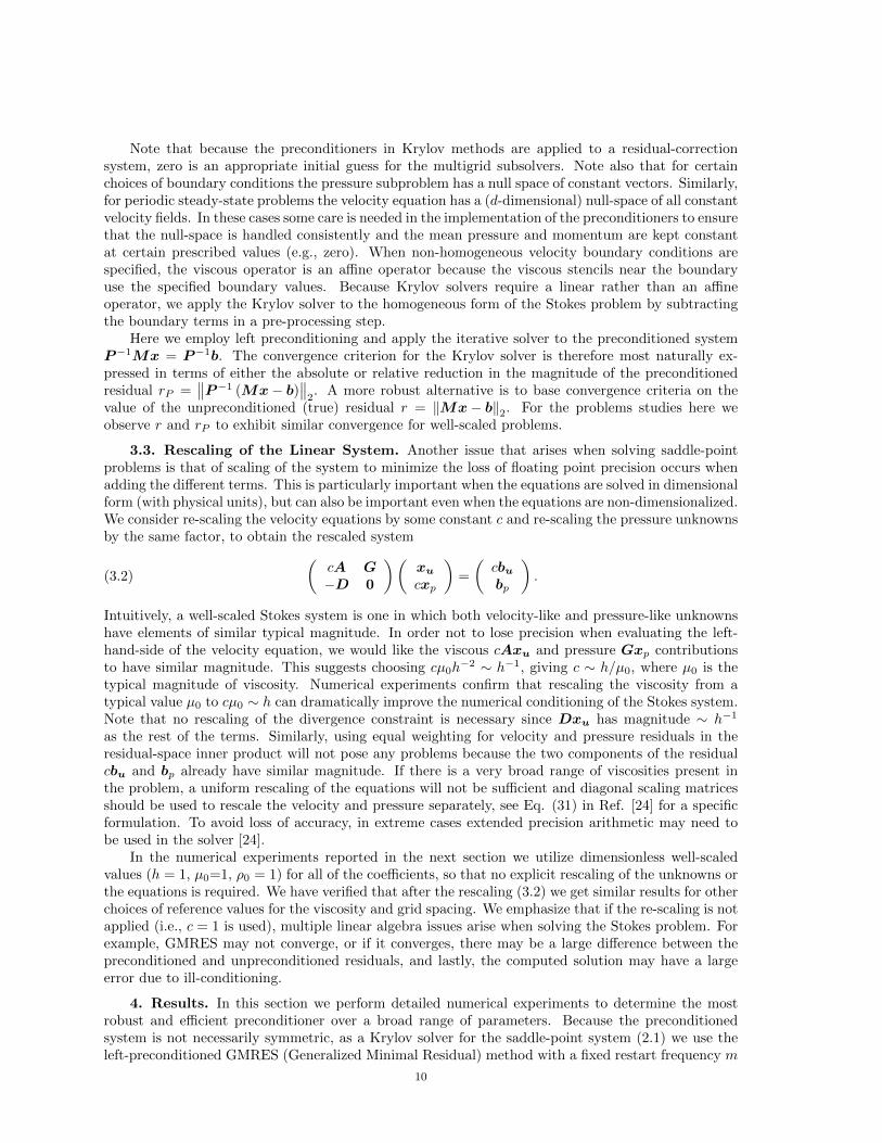
Fig. 4.1. The log of the relative residual for the pressure (left) and velocity (right) multigrid solvers as a functionof the number of multigrid V cycles, for different numbers of smoothing (relaxation) sweeps. A constant coefficientsteady Stokes problem is solved on a 5122 grid in two dimensions (top panels), and 1283 grid in three dimensions(bottom panels), with no-slip conditions at all domain boundaries.

and, more importantly, makes the smoother highly parallelizable. The optimal number of smoothing(relaxation) sweeps to be performed at each multigrid level (we use the same number of sweeps goingdown and up the multigrid hierarchy) has to be determined by numerical experimentation.

In Fig. 4.1 we show the convergence of the pressure (left panels) and velocity multigrid solvers(right panels) for constant viscosity but for the stress-tensor form of the viscous term (3.1). In theupper row we show results in two dimensions, and in the lower row we show results for three dimensions.Similar results are obtained for different types of boundary conditions. We see a large increase in therate of convergence when increasing the number of smoothing sweeps from one to two, and onlya modest increase thereafter. Since the cost of geometric multigrid is in large part dominated bysmoother, henceforth we use two applications of the smoother at each level of the multigrid hierarchyin each V cycle.

The speed of convergence of the multigrid iteration for the component solvers, is the standard

12

against which one should measure convergence of the Krylov solver for the Stokes problem. As we cansee in Fig. 4.1, each V cycle reduces the residual by at least an order of magnitude, so that only abouta dozen V cycles are needed to reduce the residual to near roundoff. Therefore, a Stokes solver thatuses only 10(d+ 1) scalar multigrid cycles to reduce the residual by more then 10 orders of magnitudeshould be considered excellent.

4.1.2. The effect of the number of multigrid cycles. As detailed in Appendix B, forconstant-coefficient Stokes problems with periodic boundaries, GMRES will converge in a single iter-ation with preconditioner P1 and in two iterations with P2 and P3. The same holds for any choice ofboundary condition for the time-dependent case in the inviscid limit. However, in the majority of casesof interest, multiple GMRES iterations will be required even if the subsolvers are exact. It is thereforeimportant to explore the use of inexact pressure and velocity solvers. Specifically, it is important todetermine the optimal number of multigrid V cycles per application of the preconditioner. We use thepreconditioner P1 for these tests; similar results are observed for all of the preconditioners.

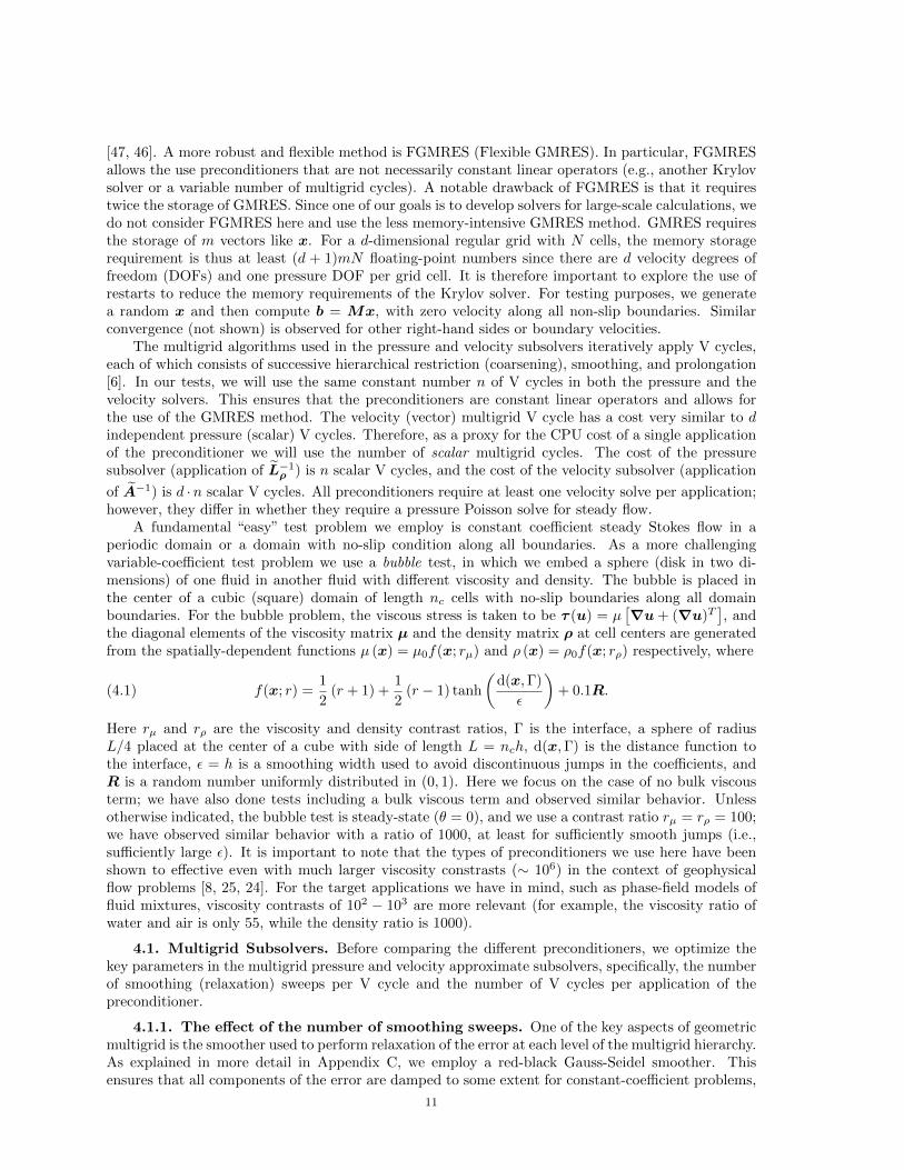
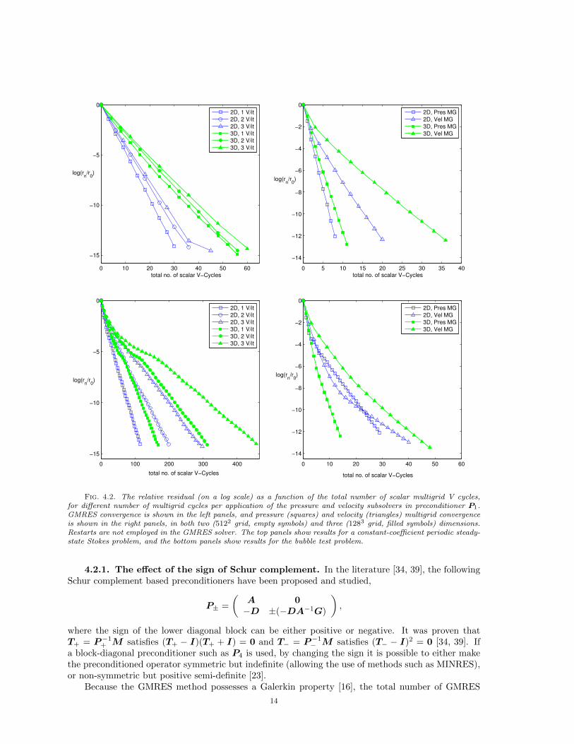
In the left panels of Fig. 4.2 we show the convergence of the relative preconditioned residual,as estimated by the GMRES algorithm, for steady Stokes problems in two and three dimensions, asa function of the total number of scalar V cycles. We recall that the number of V cycles is a goodproxy for the total computational effort, so that the most rapid convergence in these plots correspondsto the most efficient solvers. In the top left panel we show results for constant viscosity but for thestress-tensor form of the viscous term (3.1) for a periodic system, and in the bottom left panel we showresults for the variable-viscosity bubble problem described earlier. In the corresponding right panelswe show the convergence of the pressure and velocity multigrid subsolvers on the same problem, toserve as a reference point for what one may expect for a projection-like split solver.

The top left panel in Fig. 4.2 shows that for periodic constant coefficient problems there is nosignificant difference between using an exact subsolver (in effect, many V cycles per application ofthe preconditioner), and using only a single V cycle in the preconditioner but doing more GMRESiterations. This is not unexpected because the standard multigrid algorithm takes the form of a simpleRichardson iterative solver, and we expect GMRES to perform at least as well as Richardson iteration.Note that for more difficult Poisson problems, such as problems with large jumps in the coefficients, itis well-known that a Krylov solver preconditioned with multigrid is more robust than multigrid alone,see for example the discussion in Ref. [24].

In the bottom left panel in Fig. 4.2 we show the convergence of GMRES for the variable-coefficientbubble problem, which is typical of the behavior we observe when there are non-periodic boundaryconditions or variable coefficients. Similar behavior is observed for the other preconditioners (notshown). The results clearly demonstrate that when using exact subsolvers in the preconditioner doesnot yield an exact solver for the Stokes problem, the extra cost of performing more than a single Vcycle of multigrid does not pay off in terms of overall efficiency. The optimal rate of convergence isobserved when using only a single V cycle in the preconditioner. We have observed no advantageto using a different number of cycles in the pressure and velocity solvers, except for nearly inviscidproblems where performing more than one pressure cycle may be somewhat beneficial. By comparingthe left and right panels, we see that when using a single multigrid cycle in the preconditioner the totalnumber of scalar V cycles is at most 2-3 times larger than that used in fractional step (projection)methods (for example, ∼ 50 + 15 = 65 in three dimensions for projection methods as seen in the rightpanel, and ∼ 170 cycles for coupled solver as seen in the left panel).

Based on these observations, henceforth we use only a single multigrid cycle in the subsolversemployed by the preconditioners.

4.2. Comparison of Preconditioners. Having empirically determined the optimal settingsfor the pressure and velocity subsolvers, we now turn to exploring the performance of the differentpreconditioners. We begin by settling an issue regarding the proper choice of sign in the upper/lowertriangular and block-diagonal preconditioners.

13

0 10 20 30 40 50 60

−15

−10

−5

0

log(rn/r

0)

total no. of scalar V−Cycles

2D, 1 V/it

2D, 2 V/it

2D, 3 V/it

3D, 1 V/it

3D, 2 V/it

3D, 3 V/it

0 5 10 15 20 25 30 35 40

−14

−12

−10

−8

−6

−4

−2

0

log(rn/r

0)

total no. of scalar V−Cycles

2D, Pres MG

2D, Vel MG

3D, Pres MG

3D, Vel MG

0 100 200 300 400

−15

−10

−5

0

log(rn/r

0)

total no. of scalar V−Cycles

2D, 1 V/it

2D, 2 V/it

2D, 3 V/it

3D, 1 V/it

3D, 2 V/it

3D, 3 V/it

0 10 20 30 40 50 60

−14

−12

−10

−8

−6

−4

−2

0

log(rn/r

0)

total no. of scalar V−Cycles

2D, Pres MG

2D, Vel MG

3D, Pres MG

3D, Vel MG

Fig. 4.2. The relative residual (on a log scale) as a function of the total number of scalar multigrid V cycles,for different number of multigrid cycles per application of the pressure and velocity subsolvers in preconditioner P1.GMRES convergence is shown in the left panels, and pressure (squares) and velocity (triangles) multigrid convergenceis shown in the right panels, in both two (5122 grid, empty symbols) and three (1283 grid, filled symbols) dimensions.Restarts are not employed in the GMRES solver. The top panels show results for a constant-coefficient periodic steady-state Stokes problem, and the bottom panels show results for the bubble test problem.

4.2.1. The effect of the sign of Schur complement. In the literature [34, 39], the followingSchur complement based preconditioners have been proposed and studied,

P± =

(A 0−D ±(−DA−1G)

),

where the sign of the lower diagonal block can be either positive or negative. It was proven thatT+ = P−1

+ M satisfies (T+ − I)(T+ + I) = 0 and T− = P−1− M satisfies (T− − I)2 = 0 [34, 39]. If

a block-diagonal preconditioner such as P4 is used, by changing the sign it is possible to either makethe preconditioned operator symmetric but indefinite (allowing the use of methods such as MINRES),or non-symmetric but positive semi-definite [23].

Because the GMRES method possesses a Galerkin property [16], the total number of GMRES

14

iterations is equal to the degree of the characteristic polynomials of the preconditioned systems.Therefore, using both P−1

+ M and P−1− M , GMRES converges in 2 iterations if the inverses of A and

the Schur complement are exact [39]. However, when inexact subsolvers are employed, we observesignificant difference between the two choices of the sign of the Schur complement. Our numericalresults (not shown) indicate that the preconditioners with ”-” sign in front of Schur complement givealmost twice faster GMRES convergence than those with ”+” sign. This is consistent with our originalchoice in Eqs. (2.13) and (2.15).

0 10 20 30 40 50 60 70 80

−15

−10

−5

0

log(rn/r

0)

total no. of scalar V−Cycles

P1, Restart=5

P2, Restart=5

P3, Restart=5

P1, Restart=10

P2, Restart=10

P3, Restart=10

0 20 40 60 80 100 120

−15

−10

−5

0

log(rn/r

0)

total no. of scalar V−Cycles

P1, Restart=5

P2, Restart=5

P3, Restart=5

P1, Restart=10

P2, Restart=10

P3, Restart=10

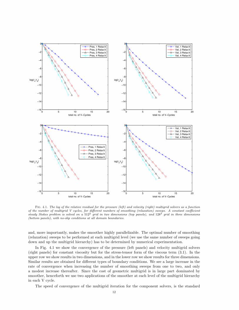
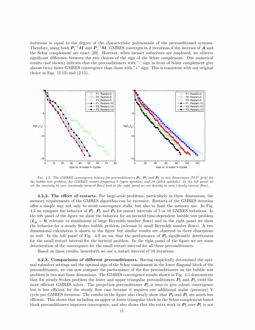
Fig. 4.3. The GMRES convergence history for preconditioners P1, P2 and P3 in two dimensions (5122 grid) forthe bubble test problem, for GMRES restart frequency 5 (open symbols) and 10 (filled symbols). In the left panel weset the viscosity to zero (unsteady inviscid flow) and in the right panel we set density to zero (steady viscous flow).

4.2.2. The effect of restarts. For large-scale problems, particularly in three dimensions, thememory requirements of the GMRES algorithm can be excessive. Restarts of the GMRES iterationoffer a simple way not only to avoid convergence stalls, but also to limit the memory use. In Fig.4.3 we compare the behavior of P1, P2 and P3 for restart intervals of 5 or 10 GMRES iterations. Inthe left panel of the figure we show the behavior for an inviscid time-dependent bubble test problem(Lµ = 0, relevant to simulations of large Reynolds number flows) and in the right panel we showthe behavior for a steady Stokes bubble problem (relevant to small Reynolds number flows). A twodimensional calculation is shown in the figure but similar results are observed in three dimensionsas well. In the left panel of Fig. 4.3 we see that the performance of P3 significantly deterioratesfor the small restart interval for the inviscid problem. In the right panel of the figure we see somedeterioration of the convergence for the small restart interval for all three preconditioners.

Based on these results, henceforth we use a restart interval of 10 iterations.

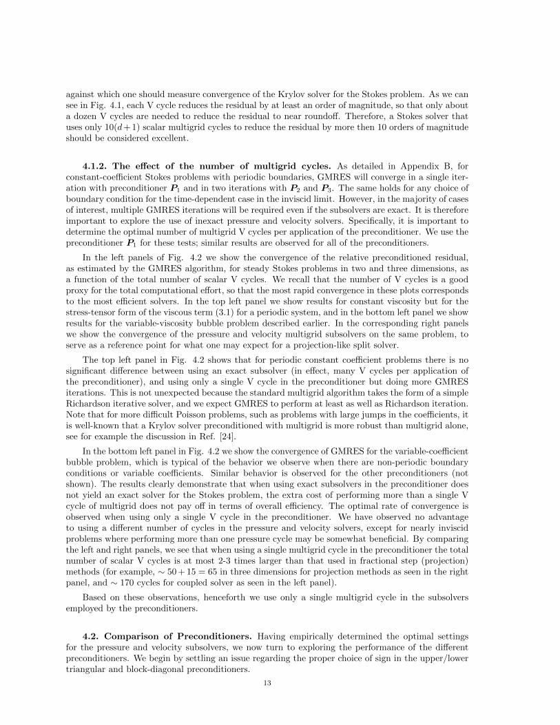
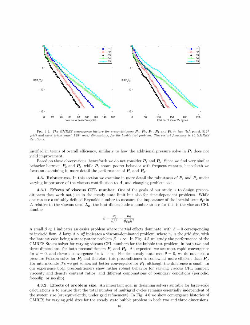
4.2.3. Comparisons of different preconditioners. Having empirically determined the opti-mal subsolver settings and the optimal sign of the Schur complement in the lower diagonal block of thepreconditioners, we can now compare the performance of the five preconditioners on the bubble testproblem in two and three dimensions. The GMRES convergence results shown in Fig. 4.4 demonstratethat for steady Stokes problem the lower and upper triangular preconditioners P2 and P3 yield themost efficient GMRES solver. The projection preconditioner P1 is seen to give robust convergencebut is less efficient for the steady flow case because it requires one additional scalar (pressure) Vcycle per GMRES iteration. The results in the figure also clearly show that P4 and P5 are much lessefficient. This shows that including an upper or lower triangular block in the Schur complement basedblock preconditioners improves convergence, and also shows that the extra work in P5 over P1 is not

15

0 20 40 60 80 100 120 140 160

−15

−10

−5

0

log(rn/r

0)

total no. of scalar V− cycles

P1

P2

P3

P4

P5

0 50 100 150 200 250

−15

−10

−5

0

log(rn/r

0)

total no. of scalar V− cycles

P1

P2

P3

P4

P5

Fig. 4.4. The GMRES convergence history for preconditioners P1, P2, P3, P4 and P5 in two (left panel, 5122

grid) and three (right panel, 1283 grid) dimensions, for the bubble test problem. The restart frequency is 10 GMRESiterations.

justified in terms of overall efficiency, similarly to how the additional pressure solve in P1 does notyield improvement.

Based on these observations, henceforth we do not consider P4 and P5. Since we find very similarbehavior between P2 and P3, while P3 shows poorer behavior with frequent restarts, henceforth wefocus on examining in more detail the performance of P1 and P2.

4.3. Robustness. In this section we examine in more detail the robustness of P1 and P2 undervarying importance of the viscous contribution to A, and changing problem size.

4.3.1. Effects of viscous CFL number. One of the goals of our study is to design precon-ditioners that work not just in the steady state limit but also for time-dependent problems. Whileone can use a suitably-defined Reynolds number to measure the importance of the inertial term θρ inA relative to the viscous term Lµ, the best dimensionless number to use for this is the viscous CFLnumber

β =ν0

θh2=

µ0

θρ0h2.

A small β 1 indicates an easier problem where inertial effects dominate, with β = 0 correspondingto inviscid flow. A large β > n2

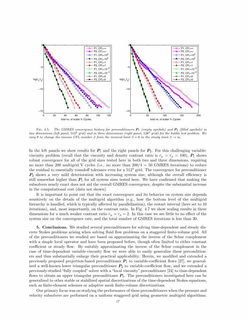
c indicates a viscous-dominated problem, where nc is the grid size, withthe hardest case being a steady-state problem β → ∞. In Fig. 4.5 we study the performance of theGMRES Stokes solver for varying viscous CFL numbers for the bubble test problem, in both two andthree dimensions, for both preconditioners P1 and P2. As expected, we see most rapid convergencefor β = 0, and slowest convergence for β → ∞. For the steady state case θ = 0, we do not need apressure Poisson solve for P2 and therefore this preconditioner is somewhat more efficient than P1.For intermediate β’s we get somewhat better convergence for P1, although the difference is small. Inour experience both preconditioners show rather robust behavior for varying viscous CFL number,viscosity and density contrast ratios, and different combinations of boundary conditions (periodic,free-slip, or no-slip).

4.3.2. Effects of problem size. An important goal in designing solvers suitable for large-scalecalculations is to ensure that the total number of multigrid cycles remains essentially independent ofthe system size (or, equivalently, under grid refinement). In Fig. 4.6 we show convergence histories ofGMRES for varying grid sizes for the steady state bubble problem in both two and three dimensions.

16

0 20 40 60 80 100 120

−15

−10

−5

0

log(rn/r

0)

total no. of scalar V−Cycles

P1, CFL=∞

P2, CFL=∞

P1, CFL=102

P2, CFL=102

P1, CFL=1

P2, CFL=1

P1, CFL=10−2

P2, CFL=10−2

P1, CFL=0

P2, CFL=0

0 50 100 150 200

−15

−10

−5

0

log(rn/r

0)

total no. of scalar V−Cycles

P1, CFL=∞

P2, CFL=∞

P1, CFL=102

P2, CFL=102

P1, CFL=1

P2, CFL=1

P1, CFL=10−2

P2, CFL=10−2

P1, CFL=0

P2, CFL=0

Fig. 4.5. The GMRES convergence history for preconditioners P1 (empty symbols) and P2 (filled symbols) intwo dimensions (left panel, 5122 grid) and in three dimensions (right panel, 1283 grid) for the bubble test problem. Wevary θ to change the viscous CFL number β from the inviscid limit β = 0 to the steady limit β →∞.

In the left panels we show results for P1 and the right panels for P2. For this challenging variable-viscosity problem (recall that the viscosity and density contrast ratio is rµ = rρ = 100), P1 showsrobust convergence for all of the grid sizes tested here in both two and three dimensions, requiringno more than 200 multigrid V cycles (i.e., no more than 200/4 = 50 GMRES iterations) to reducethe residual to essentially roundoff tolerance even for a 5123 grid. The convergence for preconditionerP2 shows a very mild deterioration with increasing system size, although the overall efficiency isstill somewhat higher than P1 for all system sizes tested here. We have confirmed that making thesubsolvers nearly exact does not aid the overall GMRES convergence, despite the substantial increasein the computational cost (data not shown).

It is important to point out that the exact convergence and its behavior on system size dependssensitively on the details of the multigrid algorithm (e.g., how the bottom level of the multigridhierarchy is handled, which is typically affected by parallelization), the restart interval (here set to 10iterations), and, most importantly, on the contrast ratio. In Fig. 4.7 we show scaling results in threedimensions for a much weaker contrast ratio rµ = rρ = 2. In this case we see little to no effect of thesystem size on the convergence rate, and the total number of GMRES iterations is less than 30.

5. Conclusions. We studied several preconditioners for solving time-dependent and steady dis-crete Stokes problems arising when solving fluid flow problems on a staggered finite-volume grid. Allof the preconditioners we studied are based on approximating the inverse of the Schur complementwith a simple local operator and have been proposed before, though often limited to either constantcoefficient or steady flow. By suitably approximating the inverse of the Schur complement in thecase of time-dependent variable-viscosity flow we were able to easily generalize these precondition-ers and thus substantially enlarge their practical applicability. Herein, we modified and extended apreviously proposed projection-based preconditioner P1 to variable-coefficient flows [27], we general-ized a well-known lower triangular preconditioner P2 to variable-coefficient flow, and we extended apreviously-studied “fully coupled” solver with a “local viscosity” preconditioner [24] to time-dependentflows to obtain an upper triangular preconditioner P3. The preconditioners investigated here can begeneralized to other stable or stabilized spatial discretizations of the time-dependent Stokes equations,such as finite-element schemes or adaptive mesh finite-volume discretizations.

Our primary focus was on studying the performance of these preconditioners when the pressure andvelocity subsolvers are performed on a uniform staggered grid using geometric multigrid algorithms.

17

0 20 40 60 80 100 120 140−16

−14

−12

−10

−8

−6

−4

−2

0

log(rn/r

0)

total no. of scalar V−Cycles

322

642

1282

2562

5122

10242

20482

0 20 40 60 80 100 120 140−16

−14

−12

−10

−8

−6

−4

−2

0

log(rn/r

0)

total no. of scalar V−Cycles

322

642

1282

2562

5122

10242

20482

0 50 100 150 200

−14

−12

−10

−8

−6

−4

−2

0

log(rn/r

0)

total no. of scalar V−Cycles

83

163

323

643

1283

2563

5123

0 50 100 150 200

−14

−12

−10

−8

−6

−4

−2

0

log(rn/r

0)

total no. of scalar V−Cycles

83

163

323

643

1283

2563

5123

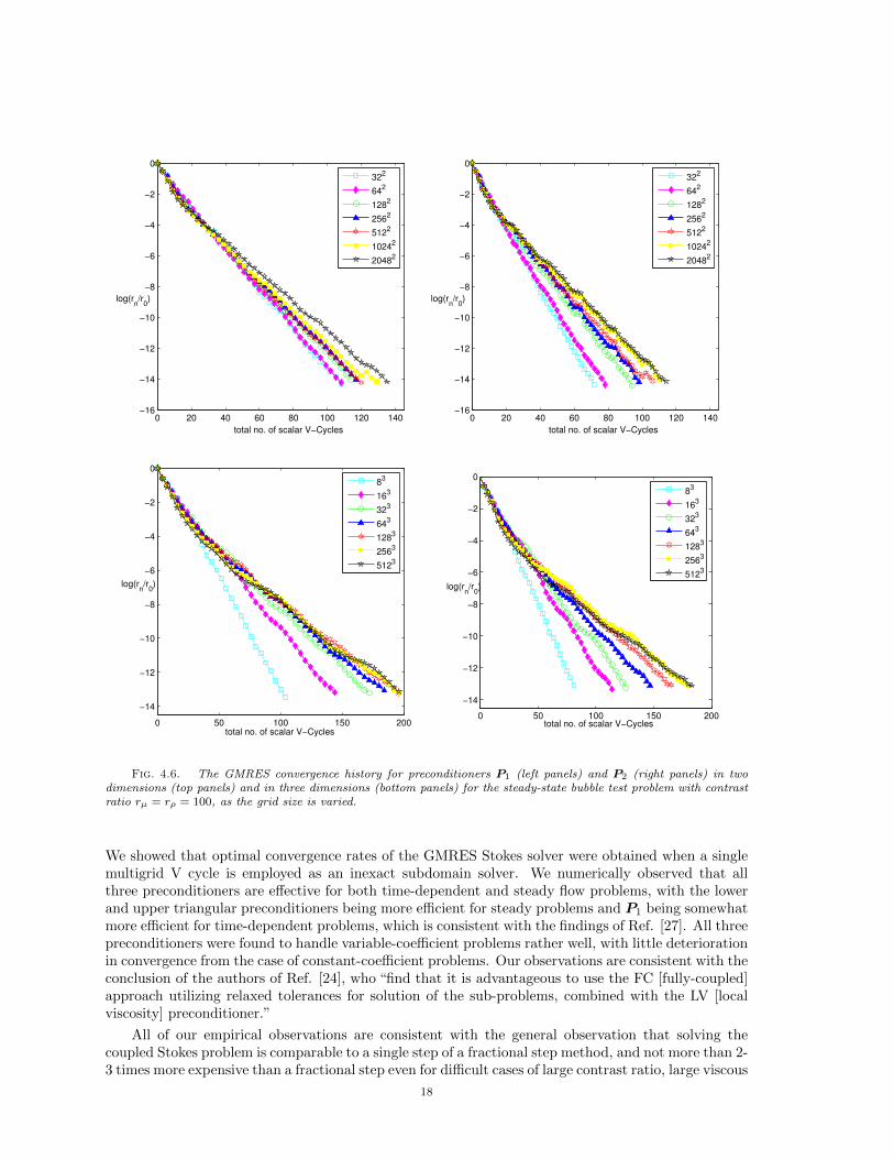
Fig. 4.6. The GMRES convergence history for preconditioners P1 (left panels) and P2 (right panels) in twodimensions (top panels) and in three dimensions (bottom panels) for the steady-state bubble test problem with contrastratio rµ = rρ = 100, as the grid size is varied.

We showed that optimal convergence rates of the GMRES Stokes solver were obtained when a singlemultigrid V cycle is employed as an inexact subdomain solver. We numerically observed that allthree preconditioners are effective for both time-dependent and steady flow problems, with the lowerand upper triangular preconditioners being more efficient for steady problems and P1 being somewhatmore efficient for time-dependent problems, which is consistent with the findings of Ref. [27]. All threepreconditioners were found to handle variable-coefficient problems rather well, with little deteriorationin convergence from the case of constant-coefficient problems. Our observations are consistent with theconclusion of the authors of Ref. [24], who “find that it is advantageous to use the FC [fully-coupled]approach utilizing relaxed tolerances for solution of the sub-problems, combined with the LV [localviscosity] preconditioner.”

All of our empirical observations are consistent with the general observation that solving thecoupled Stokes problem is comparable to a single step of a fractional step method, and not more than 2-3 times more expensive than a fractional step even for difficult cases of large contrast ratio, large viscous

18

0 20 40 60 80 100 120

−14

−12

−10

−8

−6

−4

−2

0

log(rn/r

0)

total no. of scalar V−Cycles

83

163

323

643

1283

2563

5123

0 20 40 60 80 100 120

−14

−12

−10

−8

−6

−4

−2

0

log(rn/r

0)

total no. of scalar V−Cycles

83

163

323

643

1283

2563

5123

Fig. 4.7. Same as bottom two panels of Fig. 4.6 but for contrast ratio rµ = rρ = 2.

CFL number and non-trivial boundary conditions. We believe that this mild increase in cost is morethan justified given the important advantages of the the coupled approach when solving the Navier-Stokes equations. Furthermore, we observed robust behavior of the projection and lower triangularpreconditioners for large systems with relatively frequent restarts. This demonstrates that GMRESwith preconditioners P1 and P2 provides a robust solver for large-scale computations. In future studies,the robustness of these preconditioners with respect to the variability of viscosity and density shouldbe studied more carefully. One aspect of this is whether the spectrum of the preconditioned operatorcan be provably bounded for arbitrary contrast ratios. More importantly, however, the performanceof the preconditioners in practical applications, should be accessed. Experience with steady Stokesgeodynamics applications, which have extreme viscosity contrasts, are very promising [24].

Acknowledgments. We thank Howard Elman for informative discussions. A. Donev and M.Cai were supported in part by the NSF under grant DMS-1115341. Additional support for A. Donevwas provided by the DOE Office of Science through Early Career award DE-SC0008271. B. E. Griffithacknowledges research support from the National Science Foundation under awards OCI 1047734 andDMS 1016554. J. Bell and A. Nonaka were supported by the DOE Applied Mathematics Programof the DOE Office of Advanced Scientific Computing Research under the U.S. Department of Energyunder contract No. DE-AC02-05CH11231.

Appendix A. Fourier Analysis of Schur Complement.

The most important element in the preconditioners we study here is the approximation of the Schurcomplement inverse. In previous work, Fourier analysis [9], operator mapping properties and PDEtheory in [37, 38], and commutator properties (2.4) [35, 17, 27] have been used to justify approximationsto the Schur complement inverse. Here we use Fourier analysis to justify our approximation to theSchur complement inverse for the stress form of the viscous operator (3.1). This analysis assumesperiodic boundaries but should also inform the case with physical boundary conditions.

For simplicity, we use two dimensional steady state Stokes equations for illustration but extensionsto three dimensions and time-dependent flow are trivial. We denote the discrete Fourier transform ofvelocity as v = [u, v]

T, and denote the (purely imaginary) Fourier symbol of the staggered divergence

operator as D = [Dx Dy], where Dx and Dy represent the staggered finite difference operator along

the x and y axes. The Fourier transform of the staggered gradient operator is G = −D? = [Dx Dy]T ,

19

and similarly,

Lp = DG = D2x + D2

y = −(∣∣∣Dx

∣∣∣2 +∣∣∣Dy

∣∣∣2) .Our goal is to approximate the Schur complement inverse with a Laplacian-like local operator

LS , i.e., to find (DL−1µ G)−1 = LS . This is only an approximation in general but should be exact for

periodic constant-coefficient problems. In Fourier space,

LS =(DL−1

µ G)−1

.(A.1)

When the Laplacian form of the viscous term is used, Lµ = µ0L, we have

Lµ = µ0

[D2x + D2

y 0

0 D2x + D2

y

],

which combined with (A.1) gives LS = µ0. Applying an inverse Fourier transform gives the well-knownresult LS = µ0I.

When Lµ is the discrete operator for the stress tensor form of the viscous term (3.1) and theviscosity is constant, we have

Lµ = µ0

[2D2

x + D2y DyDx

DxDy D2x + 2D2

y

],

which gives LS = 2µ0, and therefore LS = 2µ0I. This motivates our variable-viscosity generalization(2.6). When Lµ is the discrete operator for the viscous term with bulk viscosity and assuming boththe shear viscosity and the bulk viscosities are constant, we have

Lµ =

[( 4

3µ0 + γ0)D2x + µ0D

2y ( 1

3µ0 + γ0)DyDx

( 13µ0 + γ0)DxDy γ0D

2x + ( 4

3µ0 + γ0)D2y

],

which gives LS =(

43µ0 + γ0

)and therefore LS =

(4

3µ0 + γ0

)I. This motivates our variable-viscosity

generalization (2.7).

Appendix B. Analysis of preconditioners with exact subsolvers.In this Appendix we give some analysis of the spectrum of the preconditioned operators when exact

pressure and velocity subsolvers are used. To see how well the different preconditioners approximatethe original saddle point form (2.1), we formally calculate

P−11 M =

(I (I − ρ−1GL−1

ρ D)A−1G0 S−1S

),(B.1)

P−12 M =

(I A−1G0 S−1S

),(B.2)

P−13 M =

(I −A−1GS−1D A−1G

S−1D 0

),(B.3)

and lastly

P−14 M =

(I A−1G

S−1D 0

).(B.4)

20

Recall that for constant-coefficient problems with exact subsolvers, S−1 = −θρ0L−1p + µ0I. For

periodic domains, the finite-difference operators G, D, L and Lp commute,

GLp = LG and LpD = DL,(B.5)

and therefore P−11 M is exactly the discrete identity operator, and similarly, the (1,1) diagonal block

of P−13 M is zero.From (B.1), we see that the preconditioned system is block upper triangular. Therefore, the

eigenvalues of the preconditioned system are either unity or the eigenvalues of S−1S. Similarly, wecan derive the eigenvalues of the preconditioned system using (B.2) and (B.3). Alternatively, one canwrite down the generalized eigenvalue system, for instance,

M

(up

)= λP3

(up

)Again, one can see that the eigenvalues are either 1 or the eigenvalues of S−1S.

When µ0 = 0, or equivalently, ∆t → 0, we have that P−11 M = I, regardless of the boundary

conditions. If P2 is used, we have

P−12 M =

(I ∆t

ρ0G

0 I

),(B.6)

and therefore (P−12 M − I)2 = 0. This proves that in the inviscid case, the GMRES algorithm

converges in 1 iteration when preconditioner P1 is used, and in 2 iterations when P2 or P3 are used.When inexact subsolvers are used our numerical results showed that all three preconditioners exhibitexactly the same convergence rate in the inviscid case.

Furthermore, for constant viscosity (µ = 1) steady state (θ = 0) problems on a two-dimensionaldomain of nx × ny grid cells with no-slip boundaries, one can prove the following property for theeigenvalues of the Schur complement S = DL−1G:

1. λ(S) ∈ 0 ∪ [η2, 1], where η is the inf-sup constant independent of grid size [20, 41].2. The multiplicity of the 0 eigenvalue is 1.3. There are at most 2(nx − 1) + 2(ny − 1) non-unit eigenvalues of S.

This is a quantitative statement of the intuitive expectation that a few cells away from the boundariesS is close to an identity operator, just as for a periodic system (see Eq. (B.5)). The lower boundof the eigenvalues is a consequence of the uniform div-stability [19, 20, 51]. From (B.1) (and also(B.2) and (B.3)), we see that the same conclusions hold for the preconditioned systems. This analysisexplains the good performance of the simple Schur complement approximation even in the presence ofnontrivial boundary conditions [27]. Below we numerically compute the spectrum of the eigenvaluesof S−1S for both constant and variable viscosity steady flow, and confirm the theoretical predictionsabove.

B.1. Spectrum of the Preconditioned Operator. Convergence analysis of the precondi-tioned GMRES method is not straightforward and there is no simple link to the spectrum of theeigenvalues. Nevertheless, it is generally accepted and widely observed that having closely clusteredeigenvalues of the preconditioned operator P−1M leads to faster convergence. Furthermore, the ratioof the largest to the smallest eigenvalue (excluding the trivial zero eigenvalue arising from the factpressure is only determined up to a constant) should be bounded from above by a constant essentiallyindependent of grid size, and, possibly, viscosity and density contrast ratio.

We focus on the steady-flow case θ = 0 in two dimensions, for a square domain of n2c cells with

four no-slip boundaries. We consider using exact subdomain solvers, A−1 = A−1 and L−1ρ = L−1

ρ

instead of multigrid, relying on the fact that a well-designed multigrid cycle is (essentially) spectrally-equivalent to an exact solver. We explicitly form M and S−1S in MATLAB as dense matrices andcompute their eigenvalues.

In Fig. B.1, we show a histogram of the eigenvalues of the unpreconditioned and preconditionedoperators for a square domain of length nc = 32 cells with no-slip boundaries. In the upper row in Fig.

21

0 2 4 6 80

10

20

30

40

50

60

70

80

Stokes eigs

0 0.2 0.4 0.6 0.8 1 1.20

10

20

30

40

50

60

70

80

Preconditioned eigs

0 200 400 600 800 1000 1200 1400 16000

10

20

30

40

50

60

70

80

Stokes eigs

0 0.2 0.4 0.6 0.8 1 1.2 1.4 1.60

10

20

30

40

50

60

70

80

Preconditioned eigs

Fig. B.1. Histogram of the eigenvalues of M (left panels) and P−1M (more precisely, S−1S) (right panels) fora steady Stokes problem on a grid of 32× 32 cells with four no-slip boundaries. The vertical axis gives the number ofeigenvalues, truncated for the eigenvalue λ = 1 in the right panels due to the large number of unit eigenvalues. Thecase of constant viscosity is shown in the upper panels, and the case of variable viscosity with contrast ratio 100 isshown in the lower panels.

B.1 we study the constant viscosity case. The total number of DOFs isNdof = n2c+2nc (nc − 1) = 3008.

Since the original Stokes system is of saddle point type, M has both positive eigenvalues and negativeeigenvalues, and there are n2

c = 1024 eigenvalues that are smaller than or equal to zero. While theunpreconditioned spectrum shows a broad spectrum of eigenvalues with conditioning number thatgrows with the grid size, the preconditioned spectrum shows that most eigenvalues are unity, with theremaining 4 (nc − 1) /Ndof ≈ 4% nonzero eigenvalues remaining well-clustered.

In the lower row in Fig. B.1 we study the variable viscosity case for the bubble problem withviscosity contrast ratio rµ = 100. The unpreconditioned system is seen to be very badly conditioned,with a broad spectrum of eigenvalues. By contrast, the preconditioned operator is well-conditioned,with around 87% of the eigenvalues in the interval (0.99, 1.01). While some eigenvalues are larger thanunity in this case, the spread in the eigenvalues is not much different from the constant-coefficientcase. This suggests that the spectrum remains localized around unity and bounded away from zero

22

Fig. C.1. ( Left panel) The stencils for the x-component of ∇ · β∇φ (left) and ∇ · β(∇φ)T (right), in twodimensions. The black circles indicate locations of u. The black triangles indicate locations of v. The red dots indicatethe location of the β and the gradients of velocity. ( Right panel) The stencils for the x-component of ∇ · β∇v (left)and ∇ · β(∇v)T (right), in three dimensions. The black circles indicate locations of u. The black triangles indicatelocations of v and w. The red dots indicate the location of the β and the gradients of velocity.

even for rather large contrast ratios. It may be possible to extend the finite-element theory developedin Refs. [30, 29] to prove that S−1S is spectrally-equivalent to the identity matrix for the staggeredgrid discretization we employ here.

Appendix C. Multigrid algorithms.

We employ a standard V-cycle multigrid approach [6] for both the cell-centered multigrid subsolverfor the weighted Poisson operator Lρ and the staggered velocity multigrid subsolver for the viscousoperator Lµ. We use the standard residual formulation, so that on all coarsened levels we are solvingfor the error in the coarsened residual from the next-finer level. In our implementation, the multigridcoarsening factor is 2, and coarsening continues until the problem domain represented on the coarsestgrid contains two grid points (with respect to cell-centers) in any given spatial direction. At thecoarsest level of the multigrid hierarchy, we perform a large (8 or more) number of relaxations, toensure that the preconditioner is a constant linear operator.

Multigrid consists of 3 major components: (i) choice of relaxation at a particular level, (ii) coars-ening/restriction operator, and (iii) interpolation/prolongation operator.

Relaxation. Both the staggered and cell-centered solvers use multicolored Gauss-Seidel smooth-ing. The cell-centered solver uses standard red-black relaxation, whereas the staggered solver uses a2d-colored relaxation, where d is the dimensionality of the problem. Because the coupling between thedegrees of freedom corresponding to a given component of velocity is the same as for the cell-centeredPoisson equation, by coloring each component of the velocity separately, as in the standard red-blackcoloring (i.e., coloring odd grid points with a different color from the even grid points), we obtaindecoupling between the 2d colors so that each color can be relaxed separately (improving convergenceand aiding parallelization). We relax the components of velocity in turn (i.e., in three dimensions, weorder the relaxations as red-x, black-x, red-y, black-y, red-z, black-z), although other orderings of thecolors are possible. Refer to Figure C.1 for a physical representation of the viscous operator stencils.Given a cell-centered operator of the form, ∇ · β∇φ ≡ Lφ = r, or a staggered operator of the form,αφ−∇ · β[∇φ+ (∇φ)T ] ≡ Lφ = r, the relaxation takes the form

φk+1 = φk + ωD−1(r − Lφk),(C.1)

for each color in turn, where the superscript represents the iterate, and D−1 is the inverse of thediagonal elements of L. We use unit weighting factor2, ω = 1 (suggested to be near-optimal innumerical experiments) for both subsolvers.

2Note that for Jacobi relaxation with the stress form of the viscous operator, a standard analysis suggests ω = 1/2as the optimal relaxation parameter (ensuring damping of all modes).

23

Restriction. For the cell-centered solver, restriction is a simple averaging of the 2d fine cells. Forthe staggered solver, we use a slightly more complicated 6-point (d = 2) or 12-point (d = 3) stencil.For example, for x-faces we use

φci,j =

1

8

(φf

2i−1,2j + φf2i−1,2j+1 + φf

2i+1,2j + φf2i+1,2j+1

)+

1

4

(φf

2i,2j + φf2i,2j+1

)(C.2)

As seen in Figure C.1, for the staggered solver we require α at faces, and β at both cell-centers andnodes (d = 2) or edges (d = 3). When creating coefficients at coarser levels, we obtain α by averagingthe overlaying fine faces, cell-centered β by averaging the overlaying fine cell-centered values, β onnodes through direct injection, and β on edges by averaging the overlaying fine edges.

Prolongation. For the cell-centered solver, prolongation is simply direct injection from the coarsecell to the overlaying 2d fine cells. For the staggered solver, we use a slightly more complicated stencilthat involves linear interpolation for fine faces that overlay coarse faces, and bilinear interpolation forfine faces that do not overlay coarse faces. For example, for x-faces we use

φfi,j =

3

4φci/2,j/2 +

1

4φci/2,j/2−1, for i and j both even,(C.3)

φfi,j =

3

8

(φci/2,j/2 + φc

i/2+1,j/2

)+

1

8

(φci/2,j/2−1 + φc

i/2+1,j/2−1

), for i odd and j even,(C.4)

where we use integer division in the index subscripts.

REFERENCES

[1] A. S. Almgren, J. B. Bell, P. Colella, L. H. Howell, and M. L. Welcome, A conservative adaptive projectionmethod for the variable density incompressible Navier-Stokes equations, J. Comput. Phys., 142 (1998), pp. 1–46. 1, 1, 1, 1, 2, 3.2

[2] A. S. Almgren, J. B. Bell, and W. G. Szymczak, A numerical method for the incompressible Navier-Stokesequations based on an approximate projection, SIAM J. Sci. Comput., 17 (1996), pp. 358–369. 1

[3] J. B. Bell, P. Colella, and H. M. Glaz, A second order projection method for the incompressible Navier-Stokesequations, J. Comp. Phys., 85 (1989), pp. 257–283. 1, 1, 2.1

[4] M. Benzi, Preconditioning techniques for large linear systems: a survey, Journal of Computational Physics, 182(2002), pp. 418–477. 1

[5] M. Benzi, G. H. Golub, and J. Liesen, Numerical solution of saddle point problems, Acta numerica, 14 (2005),pp. 1–137. 1

[6] W. L. Briggs, V. Henson, and S. McCormick, A multigrid tutorial society for industrial and applied mathe-matics, Philadelphia, PA, (1987). 4, C

[7] D. L. Brown, R. Cortez, and M. L. Minion, Accurate projection methods for the incompressible Navier-Stokesequations, Journal of Computational Physics, 168 (2001), pp. 464–499. 1, 2

[8] C. Burstedde, O. Ghattas, G. Stadler, T. Tu, and L. C. Wilcox, Parallel scalable adjoint-based adaptivesolution of variable-viscosity stokes flow problems, Computer Methods in Applied Mechanics and Engineering,198 (2009), pp. 1691–1700. 1, 2.4, 4

[9] J. Cahouet and J.-P. Chabard, Some fast 3d finite element solvers for the generalized stokes problem, Interna-tional Journal for Numerical Methods in Fluids, 8 (1988), pp. 869–895. 2.2, 2.3, 2.4, A

[10] Z.-H. Cao, Constraint schur complement preconditioners for nonsymmetric saddle point problems, Applied Nu-merical Mathematics, 59 (2009), pp. 151–169. 2

[11] A. J. Chorin, Numerical Solution of the Navier-Stokes Equations, J. Math. Comp., 22 (1968), pp. 745–762. 1,2.1

[12] S. Delong, B. E. Griffith, E. Vanden-Eijnden, and A. Donev, Temporal Integrators for Fluctuating Hydro-dynamics, Phys. Rev. E, 87 (2013), p. 033302. 1

[13] A. Donev, T. G. Fai, and E. Vanden-Eijnden, A reversible mesoscopic model of diffusion in liquids: from giantfluctuations to Fick’s law, Journal of Statistical Mechanics: Theory and Experiment, 2014 (2014), p. P04004.1

[14] A. Donev, A. J. Nonaka, Y. Sun, T. G. Fai, A. L. Garcia, and J. B. Bell, Low Mach Number FluctuatingHydrodynamics of Diffusively Mixing Fluids, Communications in Applied Mathematics and ComputationalScience, 9 (2014), pp. 47–105. 1, 1, 3, 3.1

[15] W. E and J. Liu, Gauge method for viscous incompressible flows, Commun. Math. Sci., 1 (2003), pp. 317–332. 1[16] M. Eiermann and O. G. Ernst, Geometric aspects of the theory of krylov subspace methods, Acta Numerica, 10

(2001), pp. 251–312. 4.2.1[17] H. Elman, V. E. Howle, J. Shadid, R. Shuttleworth, and R. Tuminaro, Block preconditioners based on

approximate commutators, SIAM Journal on Scientific Computing, 27 (2006), pp. 1651–1668. 2, A

24

[18] , A taxonomy and comparison of parallel block multi-level preconditioners for the incompressible navier–stokes equations, Journal of Computational Physics, 227 (2008), pp. 1790–1808. 1

[19] H. C. Elman, Preconditioning for the steady-state navier–stokes equations with low viscosity, SIAM Journal onScientific Computing, 20 (1999), pp. 1299–1316. 1, 2, 2, B

[20] H. C. Elman, D. J. Silvester, and A. J. Wathen, Finite Elements and Fast Iterative Solvers: with Applicationsin Incompressible Fluid Dynamics: with Applications in Incompressible Fluid Dynamics, OUP Oxford, 2005.1, 1, 1, 2.4, 1, B

[21] X. Feng and Y. He, Modified homotopy perturbation method for solving the stokes equations, Computers &Mathematics with Applications, 61 (2011), pp. 2262–2266. 1

[22] X. Feng and L. Shao, On the generalized sor-like methods for saddle point problems, J. Appl. Math. Inform., 28(2010), pp. 663–677. 1

[23] B. Fischer, A. Ramage, D. J. Silvester, and A. J. Wathen, Minimum residual methods for augmented systems,BIT Numerical Mathematics, 38 (1998), pp. 527–543. 4.2.1

[24] M. Furuichi, D. A. May, and P. J. Tackley, Development of a stokes flow solver robust to large viscosity jumpsusing a schur complement approach with mixed precision arithmetic, Journal of Computational Physics, 230(2011), pp. 8835–8851. 1, 1, 2, 2, 2, 2.3, 3.3, 4, 4.1.2, 5

[25] T. Geenen, C. Vuik, G. Segal, S. MacLachlan, et al., On iterative methods for the incompressible stokesproblem, International Journal for Numerical methods in fluids, 65 (2011), pp. 1180–1200. 1, 2.3, 4

[26] T. V. Gerya, D. A. May, and T. Duretz, An adaptive staggered grid finite difference method for modelinggeodynamic Stokes flows with strongly variable viscosity, Geochemistry, Geophysics, Geosystems, 14 (2013),pp. 1200–1225. 1, 1, 1

[27] B. Griffith, An accurate and efficient method for the incompressible Navier-Stokes equations using the projectionmethod as a preconditioner, J. Comp. Phys., 228 (2009), pp. 7565–7595. 1, 1, 1, 2, 2.1, 2.1, 3, 3.1, 5, A, B

[28] , Immersed boundary model of aortic heart valve dynamics with physiological driving and loading conditions,Int J Numer Meth Biomed Eng, 28 (2012), pp. 317–345. 1, 1

[29] P. Grinevich, An iterative solution method for the stokes problem with variable viscosity, Moscow UniversityMathematics Bulletin, 65 (2010), pp. 119–122. B.1

[30] P. Grinevich and M. Olshanskii, An iterative method for the stokes-type problem with variable viscosity, SIAMJournal on Scientific Computing, 31 (2009), pp. 3959–3978. B.1

[31] J. Guermond, P. Minev, and J. Shen, An overview of projection methods for incompressible flows, ComputerMethods in Applied Mechanics and Engineering, 195 (2006), pp. 6011–6045. 3.1

[32] F. Harlow and J. Welch, Numerical calculation of time-dependent viscous incompressible flow of fluids withfree surfaces, Physics of Fluids, 8 (1965), pp. 2182–2189. 1, 3.1

[33] Q. Hu and J. Zou, Nonlinear inexact uzawa algorithms for linear and nonlinear saddle-point problems, SIAMJournal on Optimization, 16 (2006), pp. 798–825. 2.4

[34] I. C. Ipsen, A note on preconditioning nonsymmetric matrices, SIAM Journal on Scientific Computing, 23 (2001),pp. 1050–1051. 1, 2.2, 2.3, 4.2.1

[35] D. Kay, D. Loghin, and A. Wathen, A preconditioner for the steady-state navier–stokes equations, SIAM Journalon Scientific Computing, 24 (2002), pp. 237–256. 1, 2.2, 2.3, 2.4, A

[36] D. A. Kay, P. M. Gresho, D. F. Griffiths, and D. J. Silvester, Adaptive time-stepping for incompressibleflow part ii: Navier-stokes equations, SIAM Journal on Scientific Computing, 32 (2010), pp. 111–128. 2

[37] K.-A. Mardal and R. Winther, Uniform preconditioners for the time dependent stokes problem, NumerischeMathematik, 98 (2004), pp. 305–327. 1, 2.2, 2.3, 2.4, A

[38] , Preconditioning discretizations of systems of partial differential equations, Numerical Linear Algebra withApplications, 18 (2011), pp. 1–40. 1, 2.2, 2.3, 2.4, A

[39] M. F. Murphy, G. H. Golub, and A. J. Wathen, A note on preconditioning for indefinite linear systems, SIAMJournal on Scientific Computing, 21 (2000), pp. 1969–1972. 1, 2.4, 4.2.1

[40] M. Olshanskii, Multigrid analysis for the time dependent stokes problem, Mathematics of Computation, 81 (2012),pp. 57–79. 1

[41] M. A. Olshanskii and E. V. Chizhonkov, On the best constant in the inf-sup-condition for elongated rectangulardomains, Mathematical Notes, 67 (2000), pp. 325–332. 1, 3.1, 1

[42] M. A. Olshanskii, J. Peters, and A. Reusken, Uniform preconditioners for a parameter dependent saddlepoint problem with application to generalized stokes interface equations, Numerische Mathematik, 105 (2006),pp. 159–191. 1, 1

[43] R. Pember, L. Howell, J. Bell, P. Colella, W. Crutchfield, W. Fiveland, and J. Jessee, An adaptiveprojection method for unsteady, low-Mach number combustion, Combustion Science and Technology, 140(1998), pp. 123–168. 1, 1

[44] A. Quarteroni, F. Saleri, and A. Veneziani, Factorization methods for the numerical approximation of navier–stokes equations, Computer methods in applied mechanics and engineering, 188 (2000), pp. 505–526. 1

[45] C. Rendleman, V. Beckner, M. Lijewski, W. Crutchfield, and J. Bell, Parallelization of structured, hierar-chical adaptive mesh refinement algorithms, Computing and Visualization in Science, 3 (2000), pp. 147–157.Software available at https://ccse.lbl.gov/BoxLib. 3.2

[46] Y. Saad, A flexible inner-outer preconditioned gmres algorithm, SIAM Journal on Scientific Computing, 14 (1993),pp. 461–469. 4

[47] Y. Saad and M. H. Schultz, Gmres: A generalized minimal residual algorithm for solving nonsymmetric linearsystems, SIAM Journal on scientific and statistical computing, 7 (1986), pp. 856–869. 4

[48] D. Shin and J. C. Strikwerda, Inf-sup conditions for finite-difference approximations of the Stokes equations,

25

Journal of the Australian Mathematical Society-Series B, 39 (1997), pp. 121–134. 1, 3.1[49] S. Turek, Efficient Solvers for Incompressible Flow Problems: An Algorithmic and Computional Approach, vol. 6,

Springer Verlag, 1999. 1, 1[50] F. B. Usabiaga, J. B. Bell, R. Delgado-Buscalioni, A. Donev, T. G. Fai, B. E. Griffith, and C. S. Peskin,

Staggered Schemes for Fluctuating Hydrodynamics, SIAM J. Multiscale Modeling and Simulation, 10 (2012),pp. 1369–1408. 1, 3, 3.1

[51] R. Verfurth, A multilevel algorithm for mixed problems, SIAM journal on numerical analysis, 21 (1984), pp. 264–271. B

26