Efficiently Locating Photographs

in Many PanoramasMichael Kroepfl

Microsoft Corp. One Microsoft Way

Redmond, WA, 98052 +1 425 7031233

mkroepfl@microsoft.com

Yonatan Wexler Microsoft Corp.

One Microsoft Way Redmond, WA, 98052

+1 425 7064181

yonatan.wexler@microsoft.com

Eyal Ofek Microsoft Corp.

One Microsoft Way Redmond, WA, 98052

+1 425 4217050

eyalofek@microsoft.com

ABSTRACT We present a method for efficient and reliable geo-positioning of images. It relies on image-based matching of the query images onto a trellis of existing images that provides accurate 5-DOF calibration (camera position and orientation without scale). As such it can handle any image input, including old historical images, matched against a whole city. On such a scale, care needs to be taken with the size of the database. We deviate from previous work by using 360� panoramas to simultaneously reduce the database size and increase the coverage. To reduce the likelihood of false matches, we restrict the range of angles for matched features. Furthermore, we enhance the RANSAC procedure to include two phases. The second phase includes guided feature matching to increase the likelihood of positive matches. Hence, we devise a matching confidence score that separates between true and false matches. We demonstrate the algorithm on a large scale database covering a whole city in order to show its usefulness for a vision-based augmented reality system.

Categories and Subject Descriptors

H.2.8 [Spatial databases and GIS, Image databases], I.4.1 [Imaging geometry], F.2.2 [Pattern matching], I.3.7 [Virtual reality]

General Terms Algorithms, Management

Keywords Geo-Tagging, Image Matching, Location Recognition, Panorama, Augmented Reality, Urban Mapping;

1. INTRODUCTION The availability of digital cameras and online sharing in the past decade has created an abundance of collective ‘digital memories’. Pocket point-and-shoot cameras, digital SLRs, camcorders, surveillance cameras and cell phones can quickly and easily document events.

The circumstances as well as motivations for taking photographs can be numerous, either for personal or for commercial applications.

Some examples of personal uses of a camera are: documenting important moments in life, documenting places visited while traveling, or simply to capture the aesthetics of a scene. People do this either to enhance their own memory, share their experiences with other people, create art, or simply because it is virtually free these days to take photos even without an obvious reason [1].

New methods of sharing digital photographs have emerged and taken leadership during the last years. From Photo CDs and DVDs through high resolution mobile phones to digital photo frames. The web has also provided plenty of online photo sharing and social interaction websites such as Flickr [2], Facebook [3], Panoramio [4] or Photobucket [5]. These host a quickly growing collection which is larger than 10 billion photos at the time of writing.

Lately there has been a growing demand for photos which are associated with geographic locations in a process called “Geo-Tagging”. It is a useful way of organizing the information, either for personal use (“find all the photos from the vacation to Hawaii”) and commercial use (“What does that neighborhood look like?”). One common approach is to use a GPS device which captures the location (latitude and longitude) continuously using satellites or an A-GPS which also uses the cellular network. This information can be stored along with the image data (such as in the EXIF headers of the digital file) and can then be inserted into a spatial index for fast search.

The advantage of geo-tagged imagery is that it can be displayed and browsed in a more natural way. Using a map-interface with push-pins or thumbnails representing each image (or image cluster) has become the de-facto standard, rather than just displaying a linear sequence of photographs.

The use of GPS has two major drawbacks: availability and accuracy. The need to carry an extra device just for storing the location is obviously an inconvenience. Furthermore, older photographs, such as historical remains do not have such data anyways. In fact, most of the available shared photos mentioned above, are not geo-tagged. Accuracy is also a major issue. A typical consumer system can achieve up to about 5 meters of accuracy in optimal conditions. When tagging a mountain this is plenty, but in an urban setting that measurement error is too large. Moreover, GPS accuracy quickly deteriorates in urban settings due to various interference effects such as reflection (GPS “shadows”), multipath and atmospheric effects, and clock offsets.

Permission to make digital or hard copies of all or part of this work for personal or classroom use is granted without fee provided that copies are not made or distributed for profit or commercial advantage and that copies bear this notice and the full citation on the first page. To copy otherwise, or republish, to post on servers or to redistribute to lists, requires prior specific permission and/or a fee. ACM GIS '10 , November 2-5, 2010. San Jose, CA, USA (c) 2010 ACM ISBN 978-1-4503-0428-3/10/11...$10.00"

These effects result in errors of up to hundreds of meters which translate into a completely different city block or landmark. While these errors can be reduced by using differential GPS or by modeling the error behavior of GPS systems in order to reduce the uncertainty [40], remaining errors may still be too large for some applications. Other infrastructure-based geo-tagging methods use triangulation between locations of known cell phone tower positions, or local area network hotspots, which achieve even less accurate geo-positioning. Professional uses of digital cameras include news reporters, forensic evidence, surveillance cameras installed for public safety purposes, traffic and weather cameras. Online mapping websites such as Bing Maps [6] and Google Maps [7] also put an enormous effort into capturing aerial or terrestrial (“streetside”) photographs to augment their map information with photo realistic visual data.

The integration of images with maps continued with the release of Photosynth [8], which was based on the work by Snavely et al. [33] that automatically creates a 3D reconstruction of a scene by using structure from motion algorithms. It uses a collection of photographs taken from different perspectives. Functionality to geo-reference such “Synths” by aligning the point cloud derived from the 3D reconstruction, to natural features observed in an aerial view, as well as the option of exploring the Photosynth™ collection through a map interface were added later on.

While a rough geo-location of user photographs already enhances the task of exploring images by their location from a top-down view, it may not be as pleasant an experience when viewed from a “human-scale” perspective, such as within a streetside- or indoor- scene. In this case it would be desirable to have a more accurate alignment of the photograph with the underlying model - ideally pixel-accurate.

Not only could the image be observed from a perspective similar to the one from where it was taken (putting the observed scene in the context of its surrounding), but it would also be possible to augment the image by relating to it known information about the world (such as the names of streets, buildings, shops, etc.). Knowledge of a photo’s position and orientation may also enable the organization of photos into groups based on scene semantics, offering a better browsing experience of the photos [42]. This could be done either in an offline process, to more accurately geo-position a set of images, and augment them with the desired meta-information. If the process of aligning the image is fast enough, and computationally cheap, this could also be done in close to real-time, ideally on a mobile device, and be the basis for certain augmented reality (AR) scenarios.

This document describes an image based matching method, to perform the alignment of still photographs to a set of accurately positioned panorama images, representing the base-layer of the geographic world model. While the method described herein is not designed to be real-time enabled, as required for real-time AR applications, suggestions will be provided for possible ways of reducing the computational effort, and thus making the real-time goal more achievable.

One of the goals for this work was to achieve a very high matching rate, even with photographs that are substantially different from the panorama images in their appearance, due to differences in resolution, illumination, perspective, scene content, occlusions, etc., while keeping the rate of false matches as low as possible.

The paper is organized as follows. We first describe the image matching problem, followed by an overview of previous work in the areas of image based location matching and geo-localization and pose initialization for AR systems. Next we describe our algorithm in detail, and discuss the results. Finally, we will summarize our work and discuss possible future extensions and improvements.

2. PROBLEM DESCRIPTION The matching of an arbitrary query image to an existing set of images.

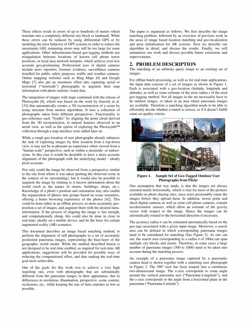
For offline-batch processing, as well as for real-time applications, the input data consists of a set of images as shown in Figure 1. Each is associated with a geo-location (latitude, longitude and altitude), as well as some estimate of the error radius r of the used geo-tagging method. Not all images in the set necessarily have to be outdoor images, or taken in an area where panorama images are available. Therefore a matching algorithm needs to be able to efficiently decide whether a match is correct, or if it doesn’t fulfill some set quality criteria.

Figure 1. Sample Set of Geo-Tagged Outdoor User Photographs from Flickr

One assumption that was made, is that the images are always oriented nearly horizontally, which is true for most of the pictures available on photo sharing sites, since users presumably rotate the images before they upload them. In addition, newer point and shoot digital cameras as well as some cell phone cameras, contain accelerometric sensors, which allow an estimate of the gravity vector with respect to the image. Hence the images can be automatically rotated to the horizontal direction if necessary.

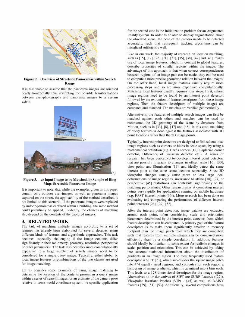
The accuracy radius r can be estimated automatically based on the geo-tags associated with a given input image. Moreover, a search area can be defined in which corresponding panorama images need to be considered for matching (See Figure 2). As one can see, the search area corresponding to a radius r of 100m can span multiple city blocks and streets. Therefore, in some cases a large number of panorama images (300 to 1000) need to be taken into account during the matching process.

An example of a panorama image captured by a panoramic camera head is shown together with a matching user photograph in Figure 3. The 360º view has been warped into a continuous two-dimensional image. The x-axis corresponds to some angle around the vertical panorama axis (“Panorama-Longitude”), and the y-axis corresponds to the angle from a horizontal plane in the panorama (“Panorama-Latitude”).

Figure 2. Overview of Streetside Panoramas within Search Range

It is reasonable to assume that the panorama images are oriented nearly horizontally thus restricting the possible transformations between user-photographs and panorama images to a certain extent.

(a)

(b)

Figure 3. a) Input Image to be Matched. b) Sample of Bing Maps Streetside Panorama Image

It is important to note, that while the examples given in this paper contain only outdoor user-images, as well as panorama images captured on the street, the applicability of the method described is not limited to this scenario. If the panorama images were replaced by indoor-panoramas captured within a building, the same method could potentially be applied. Evidently, the chances of matching also depend on the contents of the captured images.

3. RELATED WORK The task of matching multiple images according to a set of features has already been elaborated for several decades, using different kinds of features and algorithmic approaches. This task becomes especially challenging if the image contents differ significantly in their radiometry, geometry, resolution, perspective or other parameters. The task also becomes more computationally expensive if a large number of search images need to be considered for a single query image. Typically, either global or local image features or combinations of the two classes are used for image matching.

Let us consider some examples of using image matching to determine the location of the contents present in a query image within a series of search images, or an estimate of the camera pose relative to some world coordinate system. A specific application

for the second case is the initialization problem for an Augmented Reality system. In order to be able to display augmentation about the observed scene, the pose of the camera needs to be detected accurately, such that subsequent tracking algorithms can be initialized sufficiently well.

Like in our work, the majority of research on location matching, such as [15], [17], [25], [30], [31], [35], [38], [47] and [48], makes use of local image features, which, in contrast to global features, describe properties of smaller regions within the image. The advantage of this approach is that when correct correspondences between regions of an image pair can be made, they can be used to compute a more precise geometric relation between the images. On the other hand, local image features usually require more processing steps and so are more expensive computationally. Matching local features usually requires four steps. First, salient image regions need to be found by an interest point detector, followed by the extraction of feature descriptors from these image regions. Then the feature descriptors of multiple images are compared and matched. The matches are verified geometrically.

Alternatively, the features of multiple search images can first be matched against each other, and matches can be used to reconstruct the 3D geometry of the scene by Structure from Motion, such as in [33], [8], [47] and [48]. In this case, matching of query features is done against the features associated with 3D point locations rather than the 2D image points.

Typically, interest point detectors are designed to find salient local image regions such as corners or blobs in scale-space, by using a mathematical definition (e.g. Harris corners [12], Laplacian corner detector, Difference of Gaussian detector etc.). A series of research has been performed to develop interest point detectors that are possibly invariant to changes in offset, scale [16], [30], view point, and illumination [19], and ideally detect the same interest point at the same scene location repeatedly. Since 3D viewpoint changes usually cause more or less large local deformations of image regions, invariance to affine [18], [27] or perspective [45] distortions can contribute significantly to the matching performance. Other research aims at computing interest points very rapidly for applications running on mobile hardware (e.g. FAST interest points [36]). More research has been done on evaluating and comparing the performance of different interest point detectors [26], [29], [52].

After the interest point detection, image patches are extracted around each point, often considering scale and orientation parameters determined by the interest point detector, from which feature descriptors can be computed. A primary goal of the feature descriptors is to make them significantly smaller in memory footprint than the image patch from which they are computed, such that features from multiple images can be compared more efficiently than by a simple correlation. In addition, features should ideally be invariant to some extent for realistic changes in scale, position and orientation. This can be achieved by taking into account statistical information about the distribution of gradients in an image region. The most frequently used feature descriptor is SIFT [23], which sub-divides the square image patch into 4*4 equally sized regions, and computes for each region a histogram of image gradients, which is quantized into 8 bins each. This leads to a 128-dimensional descriptor for the image region. Alternatives to or derivatives of SIFT are SURF features ([27]), Viewpoint Invariant Patches (VIP) - [45] as well as DAISY features [39], [51], [53]. Additionally, several comparisons have

been done to evaluate the quality of the different feature descriptors [21], [28], [52].

Once the interest points are found, they need to be matched to the database images. The simplest matching method is by exhaustively comparing each image descriptor from the query image to each descriptor in all search images. This can be computationally very expensive, since 𝑶(𝒒 × 𝒔 × 𝒊 × 𝒅) operations are required, where q is the number of query features, s is the mean number of search features per search image, i is the number of search images, and d is the number of dimensions per feature descriptor. For q=2000, s=5000, i=300, d=128, this means that 384 billion byte comparisons need to happen. To speed up the matching process, a common method is to organize the descriptors of single or multiple images in a K-D-tree structure [9], which allows efficient nearest-neighbor search for a given query feature. This has been used by the authors of [30], [31], [33] and [48].

Even much faster feature matching can be achieved by using quantized image features, also referred to as visual words. A large number of possible image feature descriptors are clustered into a set of visual words (See [20], [34] and [38].), each of which is basically represented by a single integer number. For each search image, a list of the included words is saved, and an inverted file index can be generated which contains for each visual word a list of images in which it appears. Matching of a query image basically consists of a step that associates each feature descriptor to a corresponding visual word, and then uses the inverted file table to find possible image matches. Search images can be quickly ranked by the number of words overlapping with the query image, which is usually weighted by some a-priory likelihood for each word. Using this method, millions of images can be searched within a very short time, which makes it very attractive to large scale image search problems, such as location matching. Examples of location matching based on visual words are [38] and [49].

The last step is typically a geometric verification of the point matches, to filter out mismatches, which usually occur frequently. This is often done by using the RANSAC algorithm developed by Fischler and Bolles [10], for robust model estimation even in the case of many outliers. A variety of models, such as Fundamental Matrix, Homography, 6-DOF Pose Estimation etc. can be used to verify the geometry.

While the above order of steps is frequently used, other methods are also worth mentioning, such as a seed and spawn algorithm developed by Lilja [46], that tries to grow the matches starting from some strong seeds, by using geometric reasoning through the image space and scale space.

An alternative to local features are global image features, which contain a global description of the essence of an image (gist), derived typically by simple statistical analysis or by image understanding methods, such as color histogram information, image texture statistics or statistical descriptions of the image content.

An example of using the time-modulation of image intensity in videos recorded by stationary web-cams, by correlating it to the pattern of cloud-motion derived from satellite images, has been presented by Jacobs et al. in [41]. The major advantage of global features is the relatively high speed of matching, even in the presence of a very large number of search images (>>1M). Nevertheless, this is often outweighed by the disadvantage that

positioning can usually only be done roughly, and with a large remaining uncertainty, which renders this method inappropriate for applications such as AR.

As another alternative to using local feature descriptors for matching, edge information (edgels) can be used either to support the location matching effort, or for later pose tracking within the world model, such as shown by Reitmayr et al. [37].

Furthermore, while this paper deals with matching by using natural image features, frequently used tools for camera localization are artificial markers such as those provided by ARToolkit [55]. Artificial markers are designed to be easily detectable, even on mobile devices [22], [44], but they impose the disadvantage that localization and tracking can only work in very limited areas where markers are located.

4. OUR METHOD

4.1 Panorama Window Selection As it is the case with the majority of related work in the area of image matching, our method is based on local image features, extracted around salient image regions found by an interest point detector in different levels of an image scale space. Specifically, we are using a Laplacian interest point detector, detecting a similarity reference frame around each location (Offset, Scale and Orientation) in combination with a version of a Daisy feature descriptor with 32 dimensions developed by Winder et al. [39], [51], [53], [46].

𝜌������� = �𝐷������ − 𝐷�������

� �;𝜌������ = �𝐷������ − 𝐷������

� �

𝑖𝑓𝑓���������������

�> 𝜗:𝑅𝑒𝑗𝑒𝑐𝑡𝑀𝑎𝑡𝑐ℎ≤ 𝜗:𝐴𝑐𝑐𝑒𝑝𝑡𝑀𝑎𝑡𝑐ℎ{4.1}

(a)

(b)

Figure 4. a) Input Image with Feature Frames. b) Panorama Image with Frames and Histogram of Matches per Image

Column

After the initial pre-processing of the query images (which are resampled to be ≤ 640 Pixel in dimension, and converted into grey-scale), interest-points are detected and corresponding feature descriptors are extracted from both the query image as well as the search images. The interest point frames FQ and FP for both images are visualized in Figure 4. Then, feature matching based

purely on the feature descriptors is performed to find matching couples of descriptor vectors DQ and DP between the query image and the panorama image (See Figure 7 a for definition). This is done pairwise, by creating a K-D-tree structure from all descriptors in a given panorama image, and searching for each query feature matching features from the panorama.

To distinguish reliable matches from unreliable ones, a ratio test is performed, comparing the feature distance (in feature space) between the query descriptor and the closest and second closest descriptor from the panorama image. According to formula {4.1}, a feature pair is rejected if the ratio is above some threshold ϑ (e.g. 0.8, see [23] for reference), and accepted if the ratio is above the threshold.

Figure 5 shows the selected sub-window from the panorama image (a) as well as version of the same image warped into a virtual camera view (b). All following explanations of the algorithm are based on the assumption, that this sub-window of the panorama has already been selected, and that only the features from within this sub-window are used for further matching.

(a) (b)

Figure 5. a) Automatically Selected Sub-Window of Panorama Image; b) Unwarped Sub-Window

4.2 Orientation Constrained Matching For many applications it can be assumed, that the user photograph as well as the panorama image are not rotated around the camera axis by more than a certain angle tolerance τ. Therefore it is reasonable to assume that for the pairwise feature matching only features with reasonably similar feature orientation should be matched. Especially for streetside scenes, where repetitive structures as well as rotationally symmetrical objects can occur, this can lead to a better “signal to noise ratio” in terms of the correct matches versus incorrect matches. Figure 6 a) contains another sample pair of a query image and a panorama, for which the interest points and vectors indicating the orientation angle are shown in Figure 6 b).

Our method subdivides the features into various orientation-bins, e.g. 72 bins of 5º width each. The features within one angle bin in the query image are only matched to features within a tolerance τ from the limits of that bin. The features for the first bin, starting at 0º and ending at 5º, are shown in Figure 6 c) (Left) together with those features in the search image that are within the tolerance (Right). The same thing can be seen for a different angle bin in Figure 6 d).

Hence, the algorithm sweeps through all orientation bins, and matches only features within the right bins. Eventually, the matches for each step in the sweep are concatenated into one resulting set of point correspondences M = {{ fQ

i , fP

j }}.

a) b)

c) d)

Figure 6. Sample pair of query image (Left) and Part of Search Panorama Image (Right).

a) Original images b) Location and orientation of detected interest points c) Subset of Interest Points for a Given Orientation Window in Query Image (e.g. 0º .. 5 º) and Larger Orientation Window in Search Image (e.g. 2.5º± 10 º) d) Subset of Interest Points for a Given Orientation Window in Query Image (e.g. 200º .. 205 º) and Larger Orientation Window in Search Image (e.g. 202.5º ± 10 º)

Since the pairwise feature-based matching with a ratio test is still likely to create a large number of mismatches, a geometric verification of the matched feature pairs is required. Matching in a 3D-scene usually entails a model describing the epipolar geometry between an image pair. This may be the Fundamental-Matrix described in [24] defining the relation of each point in one image to a line in the other and vice versa. We found that for urban scenes the fundamental matrix provides too much freedom and hence allows an unacceptable amount of false positives.

We decided that for stability reasons it would be better in urban cityscapes to use a more restrictive, homography based model, which basically assumes that the object points must lie on one or more approximately flat surfaces in the 3D-scene. A homography can transform each point in one image into exactly one point in the other image, and hence is more restrictive when filtering out outliers. The advantage of using homography for image matching in urban scenes was also noted by Lourakis et al. ([14]). To estimate the homography, we use the RANSAC algorithm.

�𝑥���

𝑦���

1

� ≅ 𝐻 ∗ �𝑥��

𝑦��

1

� {4.2}

The results of RANSAC are the Homography matrix H, transforming each set of homogeneous point coordinates [ xi

Q, yiQ

, 1 ]T from the query image into a corresponding set of coordinates [ xi

Q’, yiQ’ , 1 ]T in the search image {4.2}. In addition, the

algorithm determines as a set of inlier point correspondences MI containing only those point correspondences, for which the reprojection error δij between the projected point [ xi

Q’, yiQ’ ]T

and the corresponding point from the search image [ xjP

, yjP ]T is

less than a threshold ε {4.3}.

To avoid homographies that would distort the query image in a non-desirable way, such as upside-down, mirrored, with intersecting image outlines or singularities, several checks are performed during the RANSAC process. If homography doesn’t fulfill these checks, it is declared degenerate, and the corresponding hypothesis can be rejected.

The number of inlier points ni,H for a specific homography H can be used to prune out image candidates at an early stage in the process, if they do not exceed some minimum inlier count (e.g. 20).

𝑀� = �𝑋��, 𝑋�

��; ∀𝛿�� < 𝜀; 𝛿�� = ��𝑥���

𝑦���� − �

𝑥��

𝑦���� {4.3}

4.3 Geometrically Constrained Matching Once the homography H for an image pair is known from the first matching iteration or other prior knowledge, and if the inlier count is larger than a threshold, further processing steps can be performed to confirm whether the matching hypothesis is plausible. The matching process is repeated, taking into account the projected point location for each feature point [ xi

Q’, yiQ’ ]T in

the coordinate system of the search image, as an additional pair of features for the feature matching. This means, that each query descriptor *DQ is appended with the transformed point location [ xi

Q’, yiQ’ ]T to form an extended query descriptor *DQ, and each

search descriptor DS is appended with its corresponding feature point location [ xj

P , yj

P ]T, resulting in an extended search descriptor *DP.

Hence, a new K-D-tree is generated, containing the new descriptor vectors *DP, which allows an efficient search for the nearest neighbor in the modified feature space, containing both the original feature descriptors, as well as the geometric location of the interest points.

a) b)

�𝐷��, 𝐷�

� ⋯𝐷���{𝐷�

�, 𝐷��,⋯𝐷�

� }� 𝐷��∗ , 𝐷�

�∗ ⋯ 𝐷��∗ �{ 𝐷�

�∗ , 𝐷��∗ ⋯ 𝐷�

�∗ }

𝐷�� =

⎣⎢⎢⎢⎢⎢⎢⎢⎢⎢⎡ 𝑑�

��

𝑑��

�

𝑑��

�

𝑑��

�

𝑑��

�

𝑑��

�⋮𝑑��

� ⎦⎥⎥⎥⎥⎥⎥⎥⎥⎥⎤

𝐷�� =

⎣⎢⎢⎢⎢⎢⎢⎢⎢⎢⎡ 𝑑�

��

𝑑��

�

𝑑��

�

𝑑��

�

𝑑��

�

𝑑��

�

⋮𝑑��

� ⎦⎥⎥⎥⎥⎥⎥⎥⎥⎥⎤

𝐷��∗ =

⎣⎢⎢⎢⎢⎢⎢⎢⎢⎢⎡ 𝑑�

��

𝑑��

�

𝑑��

�

𝑑��

�

𝑑��

�⋮

𝑓 ∗ 𝑥′��

𝑓 ∗ 𝑦′��⎦⎥⎥⎥⎥⎥⎥⎥⎥⎥⎤

𝐷��∗ =

⎣⎢⎢⎢⎢⎢⎢⎢⎢⎢⎡ 𝑑�

��

𝑑��

�

𝑑��

�

𝑑��

�

𝑑��

�

⋮𝑓 ∗ 𝑥�

�

𝑓 ∗ 𝑦��⎦⎥⎥⎥⎥⎥⎥⎥⎥⎥⎤

Figure 7. a) Sets { DQ } and {DP } of Feature Descriptors in Query and Search Image. b) Modified Sets {*DQ} and {*DP} of

Feature Descriptors in Query and Search Image.

For two different sample images, Figure 8 shows only those feature matches that are inliers to the RANSAC procedure for three cases: a) If only the feature descriptors are used for matching; b) With the orientation constraint in place; and c) After the second iteration, taking into account the homography to predict the geometric location of the query features in the search image.

Table 1 contains more quantitative results for the matching process, for the two images shown in Figure 6, as well as eight more images.

a)

b)

c)

Figure 8. Inliers of Feature Based Matching for Two Sample Images 1) and 2).

Row a) shows results for matching purely based on feature descriptors. Row b) shows results for matching of features with similar feature orientation. Row c) shows results for matching after second iteration, using initial homography as additional input for descriptor matching.

In Figure 8 b) it can be seen that the number of matches increases slightly if orientation constrained matching is performed. In some cases this influences whether or not an image can be matched at all. This is especially true that if the scene contains a number of rotationally symmetrical objects that could be mismatched to a rotated instance of a similar object.

A much larger number of correct matches can be achieved if the geometric location is considered during the matching process (Figure 8 c). Hence features that are closer to the expected location produce a better ratio test result, than similar but farther away features. This especially helps for cases, in which the scene contains a lot of repetitive structure, such as windows, doors, façade stucco work etc., which are frequently present in urban streetside scenes.

While the inlier count to the RANSAC operation is a strong indicator for whether or not an image should be accepted or rejected by the algorithm, there are a few more criteria to be considered for this purpose.

In addition to the Inlier Count, we collect more information about the matching process, including the distribution of the matched points in both the query and search image (represented by the Standard Deviations σQ and σP of the point coordinates), the mean Reprojection-Error 𝜹�, the mean Euclidean Feature

Distance 𝝆�between all feature pairs, as well as a Correlation Coefficient c between the two images.

Table 1. Overview of Matching Metrics for Sample Images from Figure 8 as well as 8 Further Sample Images:

Column 1 – Image Number Column 2 – Number of Features in Query Image Column 3 – Number of Features in Search Image Column 4 – Number of Matches for Purely Feature – Based Matching Column 5 – Number of Matches for Orientation - Constrained Matching Column 6 – Number of Matches for Homography Constrained Matching Column 7 – Number of RANSAC-Inliers for Purely Feature – Based Matching Column 8 – Number of RANSAC-Inliers for Orientation - Constrained Matching Column 9 – Number of RANSAC-Inliers for Homography Constrained Matching

Img Feat Query

Feat Search

M 𝑴𝝋 𝑴𝒉 I 𝑰𝝋 𝑰𝒉

1 1835 3592 103 131 317 60 73 219

2 1200 1429 63 104 204 17 26 100

3 1860 1955 166 192 316 120 139 222

4 3061 5511 50 76 191 18 24 71

5 1533 2015 82 121 303 48 60 150

6 1601 2129 37 69 272 10 13 42

7 1706 2002 204 246 454 116 126 354

8 1002 1880 33 56 77 9 12 26

9 1644 2164 133 160 319 43 50 204

10 2263 4234 58 110 172 8 13 49

To compute the correlation coefficient, the query image needs to be warped into the coordinate system of the search image by using the known homography H, as shown in Figure 9 a), and hence the area surrounding the matched feature points needs to be selected in a binary mask b). All pixel grey-values within the masked area of the two images are concatenated in a pair of vectors, which are then used to compute a correlation coefficient cg. This coefficient is expected to be close to 1.0, if the image pair matches well, and typically less than 0.6, if the image pair doesn’t match.

a) b)

Figure 9. a) Query Image Warped onto Search Image Using Homography; b) Correlation Mask around Matching Feature

Points. Correlation Coefficient for Example = 0.8609

Unfortunately, the correlation coefficient computed as above is only reliable if there are no significant illumination differences between the two images.

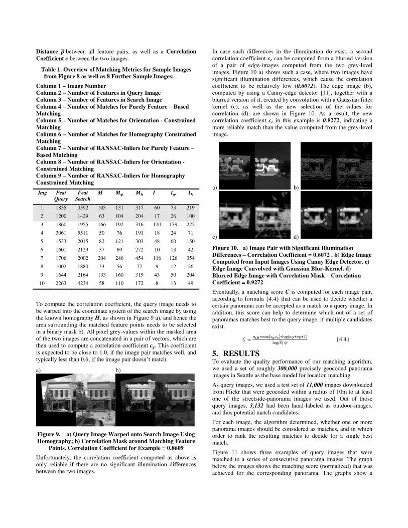
In case such differences in the illumination do exist, a second correlation coefficient ce can be computed from a blurred version of a pair of edge-images computed from the two grey-level images. Figure 10 a) shows such a case, where two images have significant illumination differences, which cause the correlation coefficient to be relatively low (0.6072). The edge image (b), computed by using a Canny-edge detector [11], together with a blurred version of it, created by convolution with a Gaussian filter kernel (c), as well as the new selection of the values for correlation (d), are shown in Figure 10. As a result, the new correlation coefficient ce in this example is 0.9272, indicating a more reliable match than the value computed from the grey-level image.

a) b)

c) d)

Figure 10. a) Image Pair with Significant Illumination Differences – Correlation Coefficient = 0.6072 . b) Edge Image Computed from Input Images Using Canny Edge Detector. c) Edge Image Convolved with Gaussian Blur-Kernel. d) Blurred Edge Image with Correlation Mask – Correlation Coefficient = 0.9272

Eventually, a matching score C is computed for each image pair, according to formula {4.4} that can be used to decide whether a certain panorama can be accepted as a match to a query image. In addition, this score can help to determine which out of a set of panoramas matches best to the query image, if multiple candidates exist.

𝐶 =��,�∗������,���∗���(�������)

���(��)∗�� {4.4}

5. RESULTS To evaluate the quality performance of our matching algorithm, we used a set of roughly 300,000 precisely geocoded panorama images in Seattle as the base model for location matching.

As query images, we used a test set of 11,000 images downloaded from Flickr that were geocoded within a radius of 10m to at least one of the streetside-panorama images we used. Out of those query images, 3,132 had been hand-labeled as outdoor-images, and thus potential match candidates.

For each image, the algorithm determined, whether one or more panorama images should be considered as matches, and in which order to rank the resulting matches to decide for a single best match.

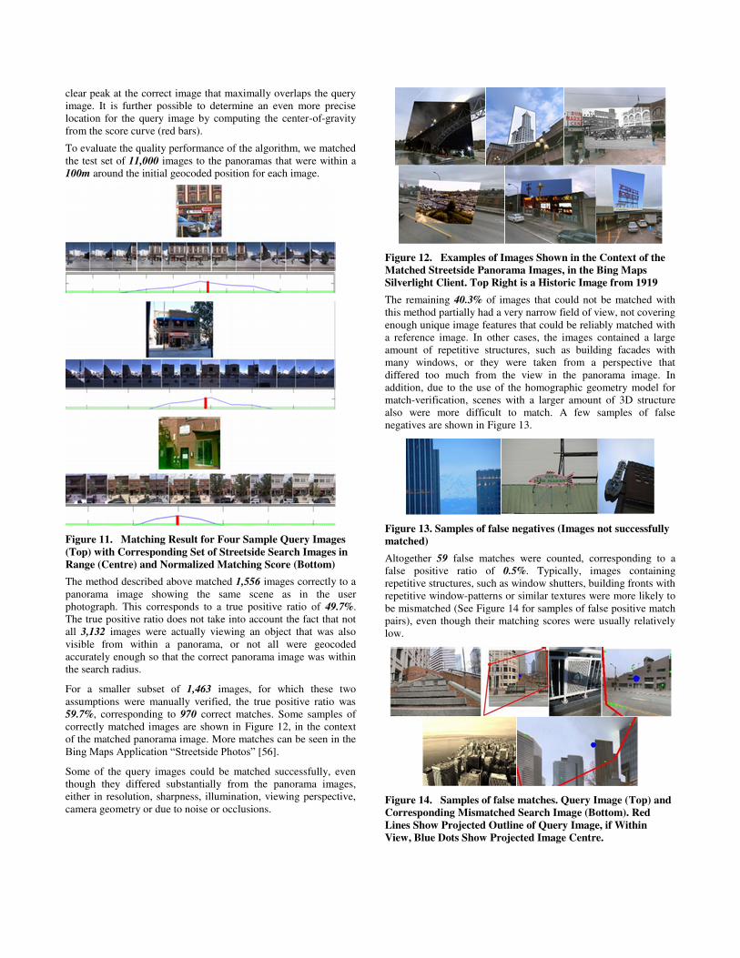
Figure 11 shows three examples of query images that were matched to a series of consecutive panorama images. The graph below the images shows the matching score (normalized) that was achieved for the corresponding panorama. The graphs show a

clear peak at the correct image that maximally overlaps the query image. It is further possible to determine an even more precise location for the query image by computing the center-of-gravity from the score curve (red bars).

To evaluate the quality performance of the algorithm, we matched the test set of 11,000 images to the panoramas that were within a 100m around the initial geocoded position for each image.

Figure 11. Matching Result for Four Sample Query Images (Top) with Corresponding Set of Streetside Search Images in Range (Centre) and Normalized Matching Score (Bottom)

The method described above matched 1,556 images correctly to a panorama image showing the same scene as in the user photograph. This corresponds to a true positive ratio of 49.7%. The true positive ratio does not take into account the fact that not all 3,132 images were actually viewing an object that was also visible from within a panorama, or not all were geocoded accurately enough so that the correct panorama image was within the search radius.

For a smaller subset of 1,463 images, for which these two assumptions were manually verified, the true positive ratio was 59.7%, corresponding to 970 correct matches. Some samples of correctly matched images are shown in Figure 12, in the context of the matched panorama image. More matches can be seen in the Bing Maps Application “Streetside Photos” [56].

Some of the query images could be matched successfully, even though they differed substantially from the panorama images, either in resolution, sharpness, illumination, viewing perspective, camera geometry or due to noise or occlusions.

Figure 12. Examples of Images Shown in the Context of the Matched Streetside Panorama Images, in the Bing Maps Silverlight Client. Top Right is a Historic Image from 1919

The remaining 40.3% of images that could not be matched with this method partially had a very narrow field of view, not covering enough unique image features that could be reliably matched with a reference image. In other cases, the images contained a large amount of repetitive structures, such as building facades with many windows, or they were taken from a perspective that differed too much from the view in the panorama image. In addition, due to the use of the homographic geometry model for match-verification, scenes with a larger amount of 3D structure also were more difficult to match. A few samples of false negatives are shown in Figure 13.

Figure 13. Samples of false negatives (Images not successfully matched)

Altogether 59 false matches were counted, corresponding to a false positive ratio of 0.5%. Typically, images containing repetitive structures, such as window shutters, building fronts with repetitive window-patterns or similar textures were more likely to be mismatched (See Figure 14 for samples of false positive match pairs), even though their matching scores were usually relatively low.

Figure 14. Samples of false matches. Query Image (Top) and Corresponding Mismatched Search Image (Bottom). Red Lines Show Projected Outline of Query Image, if Within View, Blue Dots Show Projected Image Centre.

6. CONCLUSION OUTLOOK In this paper we show that image based location matching using local features can be done reliably even in the presence of large variation in image radiometry and camera pose, due to a few key elements:

• Constraining the freedom of descriptor matching, namely by removing the rotation-invariance, as well as using only homography-based geometry verification

• Repeating the matching process after an initial homography is known to achieve a larger number of matches

• Verifying the matching hypothesis by correlating the actual images

• Computing and evaluating a matching confidence score based on the matching statistics

While our algorithm could successfully match ~60% of the verified test dataset used, the false positive ratio was only 0.5%. This performance could be achieved even though the test data included a subset of very challenging images, including images taken at night, images that were very blurry, or had only a small overlap with the panorama images. Problems occurred mostly when query images had a large number of features due to regular structures, or if the field of view of the query image was too limited and didn’t contain enough unique features to allow reliable matching.

A current weakness of the described method is that the feature matching happens for every candidate image individually, which imposes a high computational cost and makes real-time applications unfeasible. This weakness could be diminished by using a fast ranking mechanism for the candidate images, such as a global K-D-tree, which would only require a detailed verification of a subset of the images.

7. REFERENCES [1] Digital Photography,

http://en.wikipedia.org/wiki/Digital_photography#Applications_and_considerations

[2] Flickr™ http://www.flickr.com/

[3] Facebook™ http://www.facebook.com/

[4] Panoramio™ http://www.panoramio.com/

[5] Photobucket™ http://www.photobucket.com/

[6] Bing Maps™ http://www.bing.com/maps/explore/

[7] Google Maps™ http://maps.google.com/

[8] Photosynth™ htp://www.photosynth.net/

[9] J. L. Bentley, Multidimensional binary search trees used for associative searching, Communications of the ACM, Volume 18 , Issue 9, September 1975

[10] M. Fischler and R. Bolles. Random sample consensus: A paradigm for model fitting with applications to image analysis and automated cartography. Communications of the ACM, 24(6):381–395, June 1981.

[11] J. A. Canny, Computational Approach To Edge Detection, IEEE Trans. Pattern Analysis and Machine Intelligence, 8:679–714, 1986

[12] C. Harris and M. J. Stephens. A combined corner and edge detector. In Alvey Vision Conference, pages 147–152, 1988.

[13] D. G. Lowe. Object recognition from local scale invariant features. In Proc. of the International Conference on Computer Vision ICCV, Corfu, pages 1150–1157, 1999.

[14] M.1.A Lourakis, S.V. Tzurbakis, A.A. Argyros and S.C. Orphanoudakis, Using Geometric Constraints for Matching Disparate Stereo Views 3D Scenes Containing Planes. In Proc. of the International Conf. on Pat. Recogn. (ICPR'00), Vol. 1, Barcelona, Spain, Sep. 3-8, 2000.

[15] A. Baumberg. Reliable feature matching across widely separated views. In CVPR, pages 774–781, 2000.

[16] K. Mikolajczyk and C. Schmid: Indexing based on scale invariant interest points. In International Conference on Computer Vision, 525-531, 2001

[17] B. Johansson and R. Cipolla. A system for automatic pose-estimation from a single image in a city scene. In International Conference on Signal Processing, Pattern Recognition and Applications, 2002.

[18] K. Mikolajczyk and C. Schmid: An affine invariant interest point detector. In: ECCV. (2002) 128 – 142

[19] J. Matas, O. Chum, M. Urban, and T. Pajdla. Robust wide baseline stereo from maximally stable extremal regions. In Proceedings of the British Machine Vision Conference, volume 1, pages 384–393, September 2002.

[20] J. Sivic and A. Zisserman. Video Google: A text retrieval approach to object matching in videos. In ICCV, 2003.

[21] K. Mikolajczyk and C. Schmid: A performance evaluation of local descriptors. In: CVPR. Volume 2., 2003, 257 – 263

[22] D. Wagner and D. Schmalstieg. First steps towards handheld augmented reality. In 7th Intl. Symposium on Wearable Computers (ISWC’03), pages 127–137, White Plains, NY, October 2003.

[23] D. Lowe. Distinctive image features from scale-invariant key points. IJCV, 60(2):91–110, 2004.

[24] R. I. Hartley and A. Zisserman. Multiple View Geometry in Computer Vision. Cambridge University Press, ISBN: 0521540518, second edition, 2004.

[25] D. Robertson and R. Cipolla. An image-based system for urban navigation. In BMVC, 2004.

[26] F. Fraundorfer and H. Bischof. Evaluation of local detectors on non-planar scenes. In Proc. 28th workshop of the Austrian Association for Pattern Recognition, pages 125–132, 2004.

[27] T. Tuytelaars and L. V. Gool. Matching widely separated views based on affine invariant regions. IJCV, 1(59):61–85, 2004.

[28] K. Mikolajczyk and C. Schmid: A performance evaluation of local descriptors. PAMI, 27(10):1615–1630, 2005.

[29] K. Mikolajczyk, T. Tuytelaars, C. Schmid, A. Zisserman, J. Matas, F. Schaffalitzky, T. Kadir, and L. Van Gool. A comparison of affine region detectors. International Journal of Computer Vision, 65(1-2):43–72, 2005.

[30] M. Brown, R. Szeliski, and S. Winder. Multi-image matching using multi-scale oriented patches. In CVPR, volume 1, pages 510–517, 2005.

[31] D. Steedly, C. Pal, and R. Szeliski, "Efficiently Registering Video into Panoramic Mosaics," Tenth IEEE International Conference on Computer Vision (ICCV'05) Volume 1, IEEE, 2005, pp. 1300-1307.

[32] H. Bay, T. Tuytelaars, L. V. Gool: SURF: Speeded up robust features. In: European Conference on Computer Vision (2006)

[33] N. Snavely, S. Seitz, R. Szeliski. Photo tourism: exploring photo collections in 3d, SIGGRAPH, 2006.

[34] D. Nister and H. Stewenius. Scalable recognition with a vocabulary tree. In CVPR, pages 2161–2168, 2006.

[35] W. Zhang and J. Kosecka. Image based localization in urban environments. In International Symposium on 3D Data Processing, Visualization and Transmission, 2006.

[36] A. J. Chavez, A FAST interest point detection algorithm, Master of Science Thesis, 2008

[37] G. Reitmayr, T. Drummond: Going out: robust model-based tracking for outdoor augmented reality. In: ISMAR, IEEE 2006 109–118

[38] G. Schindler, M. Brown, and R. Szeliski. City-scale location recognition. In CVPR, pages 1–7, 2007.

[39] S. Winder and M. Brown. Learning local image descriptors. In CVPR, 2007.

[40] G. Reitmayr, T. Drummond: Initialization for visual tracking in urban environments. In: Proc. ISMAR 2007. 161–160

[41] N. Jacobs, S. Satkin, N. Roman, R. Speyer, R. Pless, Geolocating static cameras. In IEEE International Conference on Computer Vision (ICCV), October 2007

[42] B. Epshtein, E. Ofek, Y. Wexler, P. Zhang: Hierarchical photo organization using geo-relevance, SIGGIS 2007

[43] D. Wagner, G. Reitmayr, A. Mulloni, T. Drummond, and D. Schmalstieg. Pose tracking from natural features on mobile phones. In Proc. 7th IEEE and ACM International Symposium on Mixed and Augmented Reality (ISMAR’08), Sept. 15–18 2008.

[44] D. Wagner, T. Langlotz, and D. Schmalstieg. Robust and unobtrusive marker tracking on mobile phones. In Proc. 7th

IEEE and ACM International Symposium on Mixed and Augmented Reality (ISMAR’08), Sept. 15–18 2008.

[45] C. Wu, B. Clipp, X. Li, J.M. Frahm, M. Pollefeys: 3D Model Matching with Viewpoint Invariant Patches (VIPs). In: IEEE Conference on Computer Vision and Pattern Recognition (CVPR). (2008)

[46] S. Lilja: Matching Image Pairs, Master of Science Thesis, Stockholm, Sweden, 2008

[47] R. Castle, G. Klein, D. Murray: Video-rate Localization in Multiple Maps for Wearable Augmented Reality. ISWC 2008. 12th IEEE Symposium on Wearable Computers. Sept. 2008

[48] S. Agarwal, N. Snavely, I. Simon, S.M. Seitz, R. Szeliski: Building Rome in a day. In: IEEE International Conference on Computer Vision (ICCV). 2009

[49] A. Irschara, C. Zach, J-M. Frahm, H. Bischof: From Structure-from-Motion Point Clouds to Fast location Recognition, CVPR, 2009

[50] M. Kroepfl, E. Ofek, Y. Wexler, D. Wysocki, G. Kimchi: Geocoding by Image Matching. Microsoft Patent Application #327328.01, 2009

[51] S. Winder G. Hua, M. Brown: Picking the Best Daisy, IEEE Computer Society, June 2009

[52] A. Gil, O. M. Mozos, M. Ballesta, O. Reinoso, A comparative evaluation of interest point detectors and local descriptors for visual SLAM, Machine Vision and Applications, Springer-Verlag, March 2009

[53] M. Brown, G. Hua, S. Winder: Discriminant Learning of Local Image Descriptors. IEEE Transactions on Pattern Analysis and Machine Intelligence. February 2010

[54] E. Ofek, M. Kroepfl, J. Walker, G. Ramos, B. Aguera y Arcas: Viewing Media in the Context of Street-Level Images. Microsoft Patent Application #328899.02, 2010

[55] ARToolkit http://www.hitl.washington.edu/artoolkit/

[56] Bing Maps™ Streetside Photos CTP http://www.bing.com/maps/explore/#/bqx21pyfpdn6h2ly