Eigenmode analysis

for turbomachinery applications

Pierre Moinier∗, Michael B. Giles†

Oxford University Computing Laboratory

Oxford, United Kingdom

September 16, 2005

Abstract

This paper discusses the numerical computation of unsteady eigen-

modes superimposed upon an annular mean flow which is uniform ax-

ially and circumferentially, but non-uniform in the radial direction.

Both inviscid and viscous flows are considered, and attention is paid

to the separation of the eigenmodes into acoustic, entropy and vor-

ticity modes. The numerical computations are validated by compar-

ison to analytic test cases, and results are presented for more realis-

tic engineering applications, showing the utility of the approach for

∗Research Officer, email: moinier@comlab.ox.ac.uk†Professor, email: giles@comlab.ox.ac.uk

1

post-processing and for the construction of non-reflecting boundary

conditions.

Introduction

Turbomachinery flows are approximately time-periodic and often conceived

as the superposition of an unsteady perturbation on a steady non-uniform

mean flow. For aeroelastic analysis, it is important to accurately simulate

the features and characteristics of the unsteadiness. To achieve this, two

different approaches are typically used. The first is the solution of the un-

steady nonlinear equations using standard nonlinear time integration tech-

niques [2, 3, 5, 11, 15]. The main drawback of these methods is their high

computational cost which, in an engineering context, can constitute a major

limitation.

The second approach is linear frequency-domain analysis [8, 9, 12, 14],

which is computationally much cheaper, partly because it enables the analysis

to be performed in a single blade-to-blade passage. Based on the observation

that the dominant unsteadiness is small and time-periodic, the unsteady flow

field is decomposed into a steady non-uniform mean flow and a sum of time

periodic disturbances, each with a distinct known frequency, either a multiple

of the blade-passing frequency in forced response, or the blade vibration fre-

quency in flutter analysis. In this approach, non-periodic unsteadiness, such

as vortex shedding, is not modelled. It is assumed that this is of relatively

2

low amplitude and at a characteristic frequency which is quite distinct from

the frequencies of the aeroelastic phenomena being studied. Under these

assumptions, the flow equations are linearised in the time domain and trans-

formed into the frequency domain to eliminate the time dependency. It is

necessary to first calculate the steady flow about which the linearisation is

performed and then perform a separate linear calculation for each frequency

of interest.

Although the unsteadiness within a single blade row may be modelled on

a domain which extends indefinitely upstream and downstream of the blade

row, in practice, numerical solutions must be calculated on a truncated finite

domain. It is then important that the unsteadiness radiating away from the

blade row must not be artificially reflected at the inlet and outlet bound-

aries, in order to properly mimic the unbounded character of the far-field.

However, spurious reflections can easily be generated at boundaries, if the

numerical boundary conditions are inappropriate. To avoid the unsteady

flow solution being corrupted by non-physical reflections, Giles [4] introduced

non-reflecting boundary conditions for the 2D Euler equations. These were

generalised to the 3D Euler equations by Hall et al [10] using a mixed an-

alytical and numerical method to approximate the 3D eigenmodes. In this

approach, the unsteady flow is decomposed into upstream and downstream

propagating waves, and non-reflecting boundary conditions are enforced by

discarding the reflecting components at the far-field boundaries.

The key first step in Hall’s work is the computation of the inviscid eigen-

3

modes. In related work, Tam and Aurialt [16] have investigated the nature

of inviscid eigenmodes in swirling flow, and Cooper and Peake [1] have built

on this to perform an asymptotic analysis of the propagation of such modes

in ducts with a slowly varying radius.

The present paper addresses the extension of the approach to the 3D

Navier-Stokes equations, for which it has proved to be highly effective in

reducing the amount of reflection. The details of the non-reflecting boundary

conditions and numerical results on engineering applications will be presented

in a companion paper [13]. In this paper, the focus is on the computation of

the unsteady eigenmodes, and their use for post-processing to analyse and

visualise the propagation of acoustic energy within the domain.

Assuming that the mean flow is axially and circumferentially uniform,

the numerical method approximates the 3D eigenmodes as the eigenvectors

of a General Eigenvalue Problem (GEP) that arises from a discretisation of

the linearised Navier-Stokes equations. It will be shown that the direction of

propagation of each mode is obtained by looking at the imaginary part of the

axial wavenumbers, the eigenvalues of the GEP. The only modes propagating

upstream are acoustic eigenmodes, but there are three different families of

modes propagating downstream (acoustic, entropy and vorticity modes) and

their classification is a delicate matter. Although turbomachinery flows are

usually not uniform either in the axial or in the circumferential direction,

these assumptions are, in many cases, good enough, particularly at inflow and

outflow boundaries. For cases violating these assumptions corrections can be

4

applied so that the approach remain valid. Not relevant for the purpose of

this paper, they will be introduced in the following paper [13]. The theory

will here be applied as such, at different location inside the computational

domain and will emphasise the relevancy of the approach, as long as the

decomposition is applied away from the blade.

The paper starts with the introduction of the GEP along with the nu-

merical discretisation and followed by the analytical formulations. A method

to identify the eigenmodes is then presented and comparisons are shown for

inviscid and viscous flows in an annular duct. Finally, applications to realis-

tic geometries exemplify the effectiveness of the approach in post-processing

linear unsteady flow fields to reveal information about the propagation and

reflection of acoustic energy within turbomachinery simulations.

Inviscid Eigenmode analysis

We begin with the 3D Euler equations in conservative form and cylindrical

coordinates

∂Qc

∂t+

1

r

∂

∂r(rFr) +

1

r

∂Fθ

∂θ+

∂Fx

∂x= G . (1)

Qc denotes the conservative variables, Fr,Fθ,Fx are the fluxes in the radial,

circumferential and axial directions, and G is the source term with Coriolis

and centrifugal forces.

Linearising these equations of motion around a mean flow which is axially

5

and circumferentially uniform, yields the equation

M∂Qp

∂t+

1

r

∂

∂r(rArQp) +

1

rAθ

∂Qp

∂θ+ Ax

∂Qp

∂x= S Qp , (2)

where Qp is the vector of perturbations to the primitive variables (density,

velocity and pressure) and M = ∂Qc/∂Qp.

Because the matrices M, Ar, Aθ, Ax, S are all functions of the radius r

only, the eigenmodes are of the form

Qp = exp(iωt+imθ+ikx) Qp(r) ,

with ω being a known quantity corresponding to either the frequency of an

incoming wave (forced response) or a vibration frequency (flutter). Substi-

tuting this into Eq. (2) gives

iωMQp +1

r

∂

∂r(rArQp) +

1

rimAθQp + ikAxQp = S Qp . (3)

Discretising this on a radial grid, with a fourth-difference numerical smooth-

ing, leads to an algebraic equation of the form

(iωM + Ar + imAθ + ikAx − S

)Q = 0 , (4)

where M, Ar, Aθ, Ax and S are all matrices of dimension 5N×5N and Q a

vector of length 5N , with N being the number of radial grid points.

6

On the outer annulus, the radial velocity must be zero, and the same

condition applies also on the inner annulus for the case of annular ducts. For

cylindrical ducts, the appropriate b.c. at r=0 for the unsteady perturbations

ρ, ur, uθ, ux, p depends on the circumferential mode number m:

• m = 0 : ur = uθ = 0 ,

• m = 1 : ρ = ux = p = 0 ,

• m > 1 : ρ = ur = uθ = ux = p = 0 .

These boundary conditions are enforced by removing the corresponding rows

and columns of the matrices in Eq. (4) which in turn reduces the size of

each vector Q (e.g. for annular ducts, dim(Q) = 5N −2). This now de-

fines an eigenvalue/eigenvector problem solved using routines from the linear

algebra library LAPACK 1 to determine the axial wavenumbers k and the

corresponding eigenvectors Q.

Extension to Viscous

For viscous applications, viscous flux terms must be added to the eigenmode

analysis. In addition, the mean flow will exhibit a boundary layer profile

that the eigenmodes must take into account if one wishes an accurate modal

decomposition of the flow perturbations. Since the mean flow varies only in

the radial direction, and assuming that the Reynolds number is very large,

1www.netlib.org/lapack

7

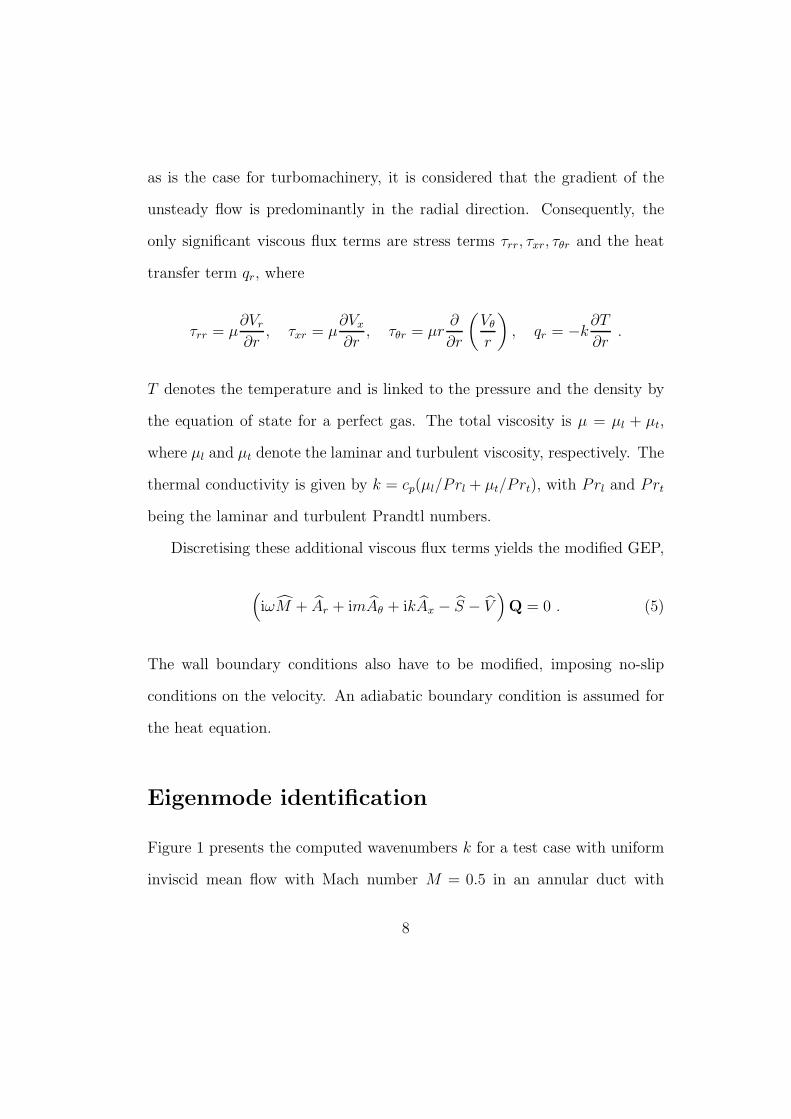
as is the case for turbomachinery, it is considered that the gradient of the

unsteady flow is predominantly in the radial direction. Consequently, the

only significant viscous flux terms are stress terms τrr, τxr, τθr and the heat

transfer term qr, where

τrr = µ∂Vr

∂r, τxr = µ

∂Vx

∂r, τθr = µr

∂

∂r

(Vθ

r

), qr = −k

∂T

∂r.

T denotes the temperature and is linked to the pressure and the density by

the equation of state for a perfect gas. The total viscosity is µ = µl + µt,

where µl and µt denote the laminar and turbulent viscosity, respectively. The

thermal conductivity is given by k = cp(µl/Prl + µt/Prt), with Prl and Prt

being the laminar and turbulent Prandtl numbers.

Discretising these additional viscous flux terms yields the modified GEP,

(iωM + Ar + imAθ + ikAx − S − V

)Q = 0 . (5)

The wall boundary conditions also have to be modified, imposing no-slip

conditions on the velocity. An adiabatic boundary condition is assumed for

the heat equation.

Eigenmode identification

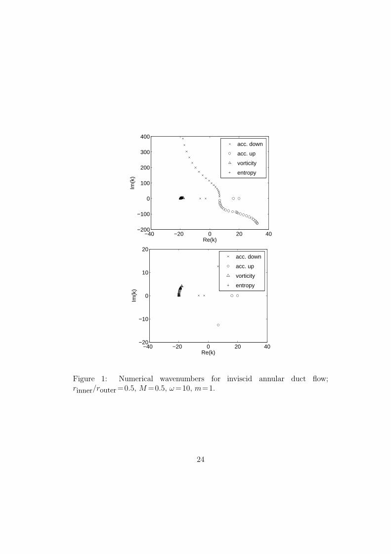
Figure 1 presents the computed wavenumbers k for a test case with uniform

inviscid mean flow with Mach number M = 0.5 in an annular duct with

8

inner/outer radius ratio λ=0.5. The frequency is ω=10, non-dimensionalised

by the outer radius and the speed of sound, and the circumferential mode

number is m=1.

The wavenumbers are each identified as belonging to one of four cate-

gories: upstream and downstream propagating acoustic modes, and down-

stream propagating entropy and vorticity modes. The purpose of this section

is to explain how this classification is performed.

Assuming physically stable modes, the upstream propagating acoustic

modes are identified in a relatively straight-forward way by looking at the

sign of the imaginary part of the wavenumbers. Considering a wave of the

form eiωt+ikx+imθ , we can re-write it as ei(ωt+krx+mθ)e−kix , where kr and ki

are the real and imaginary components of k, respectively.

If ki is positive, it corresponds to an evanescent mode with an amplitude

which decays exponentially downstream, in the direction of increasing x. This

can be considered to be a generalised downstream propagating mode, since it

corresponds to a limited downstream propagation of a disturbance introduced

at an upstream boundary. Similarly, if ki is negative, it corresponds to a

upstream propagating evanescent mode.

The difficult case, analytically, is the one in which ki is zero. In this

case, one must consider the group velocity, −∂ω/∂k. If this is positive,

then it is downstream propagating, while if it is negative it is upstream

propagating. To avoid the practical difficulty of evaluating the group velocity,

we instead introduce a small negative imaginary component to the frequency,

9

ωi = −10−5ωr, corresponding to a very slow exponential growth in time of

the eigenmode. This perturbs the wavenumber, giving ki ≈ ∂ω∂k

ωi. Thus if ki

is positive, then it is a downstream propagating mode, while if it is negative

it is an upstream propagating mode, exactly the same as for the evanescent

modes. Hence, with the introduction of the small negative ωi, the test for

the direction of propagation is simply to check the sign of ki.

This allows the identification of the upstream propagating acoustic eigen-

modes. To distinguish between the three different families of downstream

propagating modes, it is necessary to look at the eigenvectors of density (ρ),

velocity and pressure (p) perturbations at the different radial nodes. The

acoustic modes are identified on the basis that they involve significant pres-

sure perturbations. Accordingly, they are defined to be the modes with the

largest values of ||p||2, with the number of modes being equal to the number

of upstream propagating modes. In the case of annular ducts with a num-

ber of radial grid points equal to N , the number of upstream propagating

acoustic modes is N . The entropy modes are then identified as being the N

remaining modes with the largest entropy perturbations ||p − c2ρ||2, where

c is the local speed of sound of the mean flow. The rest of the modes are

defined to be vorticity modes, ie 2N − 2 for an inviscid problem and 2N − 6

for a viscous problem. The above quantification corresponds to what is ex-

pected when the flow is axially subsonic which is normal for turbomachinery

problems. For other regimes, the numbers may differ, however, the analysis

is expected to work in the same way, since the implementation does not take

10

the Mach number into account.

For physically unstable modes, such as vortex sheet instabilities or Tollmien-

Schlichting (TS) waves, the above analysis, based on the imaginary part of k,

will mis-classify them as upstream propagating modes. Although this might

cause problems, such features have not yet been encountered in practice in

turbomachinery applications.

Figure 1 shows that the classification works well, but is not perfect. An-

alytically, the entropy wavenumbers should all have value −ω/M [4], and

the results do show a very tight clustering of these wavenumbers. In the ab-

sence of the annular end-walls, the vorticity modes would all have the same

wavenumber, but the presence of the walls, and the influence of the numerical

smoothing, leads to a spreading out of the values. A couple of the vorticity

modes appear to be mis-identified as acoustic modes. These are modes with

a very rapid variation in the radial direction, and it is probably an artefact

of the numerical smoothing that causes a significant pressure variation in the

eigenmodes. There are four “cut-on” acoustic modes with ki almost zero, two

corresponding to acoustic modes propagating upstream, and two propagat-

ing downstream. The other “cut-off” acoustic modes are evanescent modes.

There are two cut-off downstream propagating acoustic modes which have

been mis-identified as entropy modes. These are modes with a very large

radial variation, leading to significant entropy production due to numerical

smoothing.

This method for classifying the eigenmodes seems to work well in real

11

turbomachinery applications, such as the ones to be presented later. How-

ever, in these applications the theoretical basis for the identification is less

solid. If mean flow has a significant swirl component (corresponding to axial

vorticity), or radial variation in the axial velocity (corresponding to circum-

ferential vorticity), then the acoustic modes have within them a significant

vortical component due to the displacement and stretching of the mean flow

vorticity [1, 16]. Similarly, the vorticity modes have an increasingly large

pressure perturbation. Nevertheless, the identification methodology appears

adequate for the purposes of both post-processing and the construction of

non-reflecting boundary conditions.

Analytic Validation

Inviscid analysis

In the case of uniform axial mean flow with Mach number M in an annular

duct, linear pressure perturbations satisfy the convected wave equation,

(∂

∂t+ M

∂

∂x

)2

p = ∇2p , λ < r < 1,

when non-dimensionalised by the uniform speed of sound and the outer duct

radius. The condition of zero radial velocity at the two endwalls leads to the

boundary conditions

∂p

∂r= 0 at r = λ, 1.

12

Looking for eigenmodes of the form

p(x, θ, r, t) = exp(ikx + imθ + iωt) P (r) ,

leads to the Bessel equation

1

r

d

dr

(rdP

dr

)+

(µ2 − m2

r2

)P = 0 , λ < r < 1 ,

where

µ2 = (ω+Mk)2 − k2 , (6)

withdP

dr= 0 on r=λ, 1. The general solution of the o.d.e. is

P (r) = a Jm(µr) + b Ym(µr) ,

where Jm and Ym are Bessel functions. The b.c.’s give

J ′

m(µλ) Y ′

m(µλ)

J ′

m(µ) Y ′

m(µ)

a

b

= 0 ,

so a non-trivial solution requires that the matrix in the above equation has

zero determinant. This yields a set of real values for µ and by solving the

quadratic Eq. (6) we obtain k.

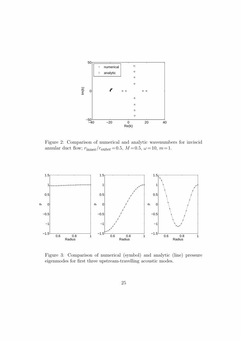
Figure 2 presents results for the same test case as Fig. 1, showing a

comparison between the computed numerical wavenumbers and the analytic

13

values for the first 12 acoustic eigenmodes, 6 in each direction.

Despite the limited number of radial points used in the discretisation,

the discretisation error is very small for all but the last two modes. Since

only the first few modes are wanted for post-processing and the construction

of non-reflecting boundary conditions, this is perfectly sufficient. Figure 3

compares the pressure component of the first 3 acoustic eigenmodes propa-

gating upstream. The agreement between the numerical and analytic values

is excellent.

Viscous analysis

In order to validate the viscous eigenmode analysis, approximate analytical

solutions of the acoustic eigenmodes for cylindrical ducts have been derived

via an asymptotic analysis which is valid at high Reynolds numbers [6]. This

asymptotic analysis breaks the domain into three regions:

• a core region in which there is a uniform mean flow, and the unsteadi-

ness is described by potential flow theory;

• a steady boundary layer region in which the mean flow is parallel and

non-uniform, and the unsteadiness is described by the linearised invis-

cid flow equations with very small normal velocity;

• a Stokes sublayer, where the mean flow is approximately stationary, and

the unsteadiness is described by the linearised viscous flow equations

with a negligible radial pressure variation and normal velocity.

14

The effect of both the steady boundary layer and the Stokes sublayer is

treated as a small perturbation to the standard eigenvalues and eigenmodes

for inviscid potential flow in a duct under the assumption that the non-

dimensional thickness of the Stokes sublayer (which is proportional to 1/√

ω Re,

where ω is the reduced frequency and Re is the Reynolds number) is much

smaller than the steady boundary layer, which in turn is much smaller than

unity, which is the non-dimensional radius of the duct.

The viscous test case considers unsteadiness of frequency ω = 10 in a

cylindrical duct with a core flow of uniform Mach number 0.5. The Reynolds

number is chosen to have the extremely high value of 2.5×1010 to ensure that

the Stokes sublayer is much thinner than the steady boundary layer which

has thickness 0.002. This clear separation of length scales between the core

flow, the steady boundary layer and the Stokes sublayer is important for the

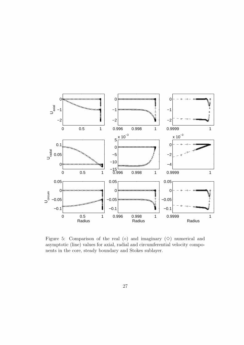
asymptotic analysis. Figure 4 shows the steady boundary layer profile next to

the outer annulus, and a comparison of the computed and asymptotic pres-

sure component of the first radial eigenmode. Figure 5 shows a comparison

of the corresponding computed and asymptotic values for the real and imag-

inary velocity components, with blow-ups showing the excellent agreement

in the steady boundary layer and the Stokes sublayer.

The final validation comes from a comparison of the change in the wavenum-

ber due to the steady boundary layer and viscous effects, taking the difference

between the viscous wavenumber value and the corresponding value from in-

viscid analysis without the steady boundary layer. The computed difference

15

is −0.0364 − 0.00028i, while the asymptotic value is −0.0373 − 0.00031i. It

can be proved that the real part is primarily due to the steady boundary

layer, while the imaginary part is due to the Stokes sublayer. The agreement

is again good, giving confidence in both the numerical evaluation and the

asymptotic analysis.

Eigenmode decomposition

Under the assumption that the mean flow is axisymmetric, a general un-

steady flow solution with a given frequency ω can be represented as a sum

of eigenmodes,

Q(x, r, θ, t) =∑

m,n

amn(x) exp(iωt+imθ) umn(r). (7)

This is a double summation, over the circumferential mode number m and the

radial modes n which exist for each value of m. The modal amplitude mode

amn will be proportional to exp(ikmnx), where kmn is the axial wavenumber.

Given such a flow solution Q(x, r, θ, t) computed by a linear frequency-

domain analysis as described in the Introduction, the eigenmode decomposi-

tion at a particular axial location x0 begins by performing a circumferential

Fourier transform of the data to obtain the quantities Qm defined by

Q(x0, r, θ, t) =∑

m

exp(iωt+imθ) Qm(x0, r).

16

From this it follows that

Qm(x0, r) =∑

n

amn(x0) umn(r).

If Qm(x0, r) and the eigenmodes umn(r) are sampled at the same set of

discrete radial nodes, then the discrete version of this equation is

Qm(x0) = Amam(x0),

where am is the vector of modal amplitudes for the different radial modes cor-

responding to circumferential mode m, and Am is the matrix whose columns

are the corresponding discrete eigenvectors. If the number of radial eigen-

modes is chosen so that Am is a square matrix, this can be inverted to obtain

am(x0) = (Am)−1Qm(x0).

Repeating this process for each circumferential mode and at differential axial

locations enables one to plot the modal amplitudes amn(x) as a function of

axial distance.

The above description is for the post-processing of results obtained from

linear frequency-domain solutions. Two such applications are presented in

the next section. In the case of nonlinear time-domain calculations, it would

be necessary to perform an additional Fourier decomposition in time, to

separate out the different frequencies in the solution, and then each of these

17

could be treated as described above.

Applications

The first numerical example concerns a cascade of flat plate stator vanes in

an annular duct, as depicted in Fig. 6. The mean flow is inviscid and uniform

with the velocity purely in the axial direction. The unsteadiness is due to

an analytically defined vortical wave introduced at the inlet of the domain.

This problem is known as the category 4 benchmark problem from the 3rd

Computational Aeroacoustics Workshop on Benchmark Problems [17]). The

results in Fig. 7 show the sound pressure level (SPL2) evaluated at the

outer wall of the duct, for the first radial acoustic harmonic of a standard

linear computation for Fourier modes −32,−8, 16 and 64. The incident wave

corresponds to circumferential mode 16. Since there are 24 blades in the

cascade, the interaction generates a response solely in modes m = 16+24p

for integer p.

The harmonic decomposition shows a combination of both propagating

and evanescent modes upstream and downstream of the flat plate located

at 0 < x < 0.1. The modes with approximately constant amplitude are

the “cut-on” propagating modes; analytically, their amplitudes should be

perfectly constant. The modes with amplitudes which appear to be almost

linear in this logarithmic plot are the”cut-off” evanescent modes; the linear

220 times the logarithm to the base 10 of the ratio of R.M.S. sound pressure to thereference sound pressure.

18

logarithmic behaviour corresponds to the expected exponential decay of the

modes. The most important point of interest is that the unsteady interaction

produces a mode 40 downstream-propagating acoustic wave which is reflected

at the downstream boundary into a mode 40 upstream-propagating acoustic

wave. There is also a very strong reflection in Fourier mode 16; in this case

this is a consequence of the outgoing vortical mode which is not plotted. The

reflected mode decays very rapidly away from the boundary and so does not

contaminate the computed solution in the neighbourhood of the blade.

The second example concerns the unsteady viscous flow around a turbine

outlet guide vane (OGV), shown in Fig. 8, due to an incoming acoustic

wave in Fourier mode −10. Fig. 9a) shows the SPL level of the first radial

harmonic for Fourier modes −28,−10, 8 and 16 when using standard quasi-

1D non-reflecting boundary conditions. All of the acoustic modes are cut-

on, upstream and downstream of the blade located in the region 0.64 <

x < 0.84. Downstream of the blade, there can be seen four acoustic modes

propagating downstream, and two propagating back upstream as a result of

spurious reflections. These reflections are in the two higher circumferential

harmonics for which the quasi-1D non-reflecting boundary conditions are

much less effective. Upstream of the blade there are three modes propagating

upstream, and two propagating downstream, one of which is the original

input disturbance and the other is another spurious reflection. Fig. 9b) shows

the great improvement that is achieved through the use of 3D non-reflecting

boundary conditions. There is now no spurious reflection at either the inflow

19

or the outflow boundaries. The decomposition shown is performed outside

the blade location, up to a point, near the blade, where the assumptions

are clearly violated. Despite that, the amplitude of the propagation modes

remain relatively constant, showing that the error made is quite small.

Conclusions

In this paper we have described a numerical method for computing unsteady

inviscid and viscous eigenmodes in annular ducts with a mean flow which is

axially and circumferentially uniform, but can vary radially. The method has

been validated by comparison with analytic and asymptotic results for model

problems, and then used in two engineering applications as a post-processing

tool to display the amplitude of different acoustic modes propagating up-

stream and downstream of turbomachinery blade rows.

One use of this tool is to identify spurious reflections of outgoing eigen-

modes. The extension of this work leads naturally to the implementation

of 3D non-reflecting boundary conditions to suppress such reflections. This

will be covered in detail in a second paper but one set of results has been

included here to show its effectiveness.

20

References

[1] Cooper, A.J., and Peake, N., “Propagation of unsteady disturbances

in a slowly varying duct with mean swirling flow”, Journal of Fluid

Mechanics, 445:207–234, 2001.

[2] Erdos, J.I., Alzner, E., and McNally, W., “Numerical solution of periodic

transonic flow through a fan stage”, AIAA Journal, 15(11):1559, 1977.

[3] Gerolymos, G.A., “Advances in the numerical integration of the three-

dimensional Euler equations in vibrating cascades”, AIAA Journal of

Propulsion and Power, 115(4):356–362, 1993.

[4] Giles, M.B., “Non-reflecting boundary conditions for Euler equation

calculations”, AIAA Journal, 28(12):2050–2058, 1990.

[5] Giles, M.B., “Stator/rotor interaction in a transonic turbine”, AIAA

Journal of Propulsion and Power, 6(5):621–627, 1990.

[6] Giles, M.B., and Moinier, P., “Asymptotic analysis of viscous acoustic

eigenmodes”, In preparation, 2004.

[7] Hall, K.C., “Deforming grid variational principle for unsteady small

disturbance flows in cascades”, AIAA Journal, 31(5):891–900, 1993.

[8] Hall, K.C., and Crawley, E.F., “Calculation of unsteady flows in tur-

bomachinery using the linearized Euler equations”, AIAA Journal,

27(6):777–787, Jun 1989.

21

[9] Hall, K.C., and Lorence, C.B., “Calculation of three-dimensional un-

steady flows in turbomachinery using the linearized harmonic Euler

equations”, Journal of Turbomachinery, 115:800–809, October 1993.

[10] Hall, K.C., Lorence, C.B., and Clark, W.S., “Non-reflecting boundary

conditions for linearized unsteady aerodynamic calculations”, AIAA

Paper 93-0882, 1993.

[11] He, L., and Denton, J.D., “3-dimensional time-marching inviscid and

viscous solutions for unsteady flows around vibrating blades”, Journal

of Turbomachinery, 116(3):469–476, 1994.

[12] Lindquist, D.R., and Giles, M.B., “Validity of linearized unsteady Euler

equations with shock capturing”, AIAA Journal, 32(1):46, 1994.

[13] Moinier, P. and Giles, M.B., “Non-reflecting boundary conditions for

3D viscous flows in turbomachinery”, In preparation, 2004.

[14] Ni, R.H., and Sisto, F., “Numerical computation of nonstationary aero-

dynamics of flat plate cascades in compressible flow”, Journal of Engi-

neering for Power, 98:165–170, 1976.

[15] Rai, M.M., “Navier-Stokes simulations of rotor-stator interaction using

patched and overlaid grids”, AIAA Journal of Propulsion and Power,

3(5):387–396, 1987.

[16] Tam, C.K., and Auriault, L., “The wave modes in ducted swirling flows

with mean swirling flow”, Journal of Fluid Mechanics, 371:1–20, 1998.

22

[17] Third computational aeroacoustics workshop on benchmark problems.

Ohio Aerospace Institute,Brook Park/Cleveland,Ohio, November 1999.

23

−40 −20 0 20 40−200

−100

0

100

200

300

400

Re(k)

Im(k

)

acc. down

acc. up

vorticity

entropy

−40 −20 0 20 40−20

−10

0

10

20

Re(k)

Im(k

)

acc. down

acc. up

vorticity

entropy

Figure 1: Numerical wavenumbers for inviscid annular duct flow;rinner/router=0.5, M =0.5, ω=10, m=1.

24

−40 −20 0 20 40−50

0

50

Re(k)

Im(k

)

numerical

analytic

Figure 2: Comparison of numerical and analytic wavenumbers for inviscidannular duct flow; rinner/router=0.5, M =0.5, ω=10, m=1.

0.6 0.8 1−1.5

−1

−0.5

0

0.5

1

1.5

Radius

p

0.6 0.8 1−1.5

−1

−0.5

0

0.5

1

1.5

Radius

p

0.6 0.8 1−1.5

−1

−0.5

0

0.5

1

1.5

Radius

p

Figure 3: Comparison of numerical (symbol) and analytic (line) pressureeigenmodes for first three upstream-travelling acoustic modes.

25

0.998 0.9985 0.999 0.9995 10

0.2

0.4

0.6

0.8

1Near wall axial velocity profile

Radius0 0.5 1

−0.5

0

0.5

1

1.5Pressure

Radius

Figure 4: Steady boundary layer velocity profile, and comparison of numeri-cal (symbol) and asymptotic (line) pressure eigenmode for viscous test case.

26

0 0.5 1

−2

−1

0

Uax

ial

0.996 0.998 1

−2

−1

0

0.9999 1

−2

−1

0

0 0.5 1

0

0.05

0.1

Ura

dial

0.996 0.998 1−15

−10

−5

0

5x 10

−3

0.9999 1

−4

−2

0

x 10−3

0 0.5 1

−0.1

−0.05

0

0.05

Radius

Uci

rcum

0.996 0.998 1

−0.1

−0.05

0

0.05

Radius0.9999 1

−0.1

−0.05

0

0.05

Radius

Figure 5: Comparison of the real (◦) and imaginary (3) numerical andasymptotic (line) values for axial, radial and circumferential velocity compo-nents in the core, steady boundary and Stokes sublayer.

27

Figure 6: Inviscid annular cascade: geometry and surface grid.

28

BLADE

X

SPL (dB)

-0.20 0.00 0.20 0.40 120.

140.

160.

Figure 7: Inviscid annular cascade: amplitude of the first ra-dial harmonic acoustic mode propagating upstream (straight line)and downstream (dashed line) for circumferential Fourier modes−32(3),−8(×), 16(△), 40(◦) and 64(2).

29

Figure 8: Viscous turbine OGV: geometry and surface grid.

30

BLADE

X

SPL (dB)

0.50 0.70 0.90 1.10 115.0

125.0

135.0

a) quasi-1D non-reflecting b.c.’s

BLADE

X

SPL (dB)

0.50 0.70 0.90 1.10 115.0

125.0

135.0

b) 3D non-reflecting b.c.’s

Figure 9: Viscous turbine OGV: amplitude of the first radial harmonic acous-tic mode propagating upstream (straight line) and downstream (dashed line)for circumferential Fourier modes −28(3),−10(△), 8(◦) and 26(2).

31