Eindhoven University of Technology MASTER Adaptive edge detection and line extraction for the Vision Survey System Brouwer, A.R. Award date: 1994 Link to publication Disclaimer This document contains a student thesis (bachelor's or master's), as authored by a student at Eindhoven University of Technology. Student theses are made available in the TU/e repository upon obtaining the required degree. The grade received is not published on the document as presented in the repository. The required complexity or quality of research of student theses may vary by program, and the required minimum study period may vary in duration. General rights Copyright and moral rights for the publications made accessible in the public portal are retained by the authors and/or other copyright owners and it is a condition of accessing publications that users recognise and abide by the legal requirements associated with these rights. • Users may download and print one copy of any publication from the public portal for the purpose of private study or research. • You may not further distribute the material or use it for any profit-making activity or commercial gain
Transcript
Eindhoven University of Technology
MASTER
Adaptive edge detection and line extraction for the Vision Survey System
Brouwer, A.R.
Award date:1994
Link to publication
DisclaimerThis document contains a student thesis (bachelor's or master's), as authored by a student at Eindhoven University of Technology. Studenttheses are made available in the TU/e repository upon obtaining the required degree. The grade received is not published on the documentas presented in the repository. The required complexity or quality of research of student theses may vary by program, and the requiredminimum study period may vary in duration.
General rightsCopyright and moral rights for the publications made accessible in the public portal are retained by the authors and/or other copyright ownersand it is a condition of accessing publications that users recognise and abide by the legal requirements associated with these rights.
• Users may download and print one copy of any publication from the public portal for the purpose of private study or research. • You may not further distribute the material or use it for any profit-making activity or commercial gain
Eindhoven University of TechnologyDepartment of Electrical EngineeringMeasurement and Control Section
Adaptive edge detectionand line extraction for the
Vision Survey System
A.R. Brouwer
M.Sc. Thesis,carried out from December 1993 to June 1994.
Commissioned by prof.dr.ir. P.P.J. v.d. Bosch,under supervision of ir. M. Hanajfk and ir. N.G.M. Kouwenberg.
The Department of Electrical Engineering of the Eindhoven University of Technologyaccepts no responsibility for the contents of M.Sc. Theses or reports on practical trainingperiods.
Abstract
Brouwer, A.R.; Adaptive edge detection and line extraction for the vision surveysystem.M.Sc. Thesis, Measurement and Control Section ER, Department of Electrical Engineering, Eindhoven University of Technology, The Netherlands, June 1994.
A Vision Survey System is being designed as a part of an intelligent robot welding system. The VSS usesCCD cameras to generate a geometrical scene description with the aid of knowledge based object modeldescriptions. Subtasks of the VSS are camera calibration, low-level vision operations, structural andgeometrical matching and object part clustering. A synthetic image modeler is applied for verificationpurposes. The subjects of this thesis are the low-level vision module algorithms and the design andimplementation of a user interface for the VSS.Output of the low-level vision module is a set of line-segments. These are obtained from a grey-level inputimage by performing lens correction, edge detection, line extraction and post-processing in succession. Thetask of edge detection is marking locations where changes in the brightness of the image occur. The lineextraction algorithm attempts to fit straight lines through these so-called edgepixels. Schemes are proposed toautomatically set optimal values for some edge detection parameters. Application of a post-processingalgorithm condenses the number of lines and enhances their accuracy. The edge detection algorithm wasimproved by combining brightness information from different images, obtained with different lightingconditions.A user interface has been implemented using MS-Windows 3.1. A separation has been made between thecoding of the VSS algorithms (non- windows) and their graphical output and parameter settings. These I/Ofunctions are handled by the user-interface.
Samenvatting
Brouwer, A.R.; Adaptive edge detection and line extraction for the vision surveysystem.Afstudeerverslag, vakgroep Meten en Regelen (ER), Faculteit Electrotechniek, TechnischeUniversiteit Eindhoven, juni 1994.
Een Vision Survey Systeem wordt ontwikkeld als onderdeel van een robot lassysteem. Ret VSS gebruiktCCD camera's om met behulp van kennissysteem objectmodellen een geometrische scene beschrijving op testellen. Onderdelen van het VSS zijn camera calibratie, low-level vision operaties, structural en geometricalmatchen en object part clustering. Een synthetische beeldmodellering wordt gebruikt om het resultaat teverifieren. De onderwerpen van dit verslag zijn de low-level vision module algoritmen en het ontwerp en deimplementatie van een gebruikersinterface voor het VSS.Uitvoer van de low-level vision module is een verzameling lijnstukken. Deze zijn verkregen van eengrijswaardenbeeld door achtereenvolgens toepassen van lenscorrectie, edgedetectie, lijnextractie enpostprocessing. De taak van edgedetectie is het markeren van plaatsen waar veranderingen in de helderheidvan het beeld voorkomen. Ret lijnextractie algoritme poogt vervolgens om rechte lijnen door deze zgn.edgepixels te passen. Een methode om automatisch de optimale waarden voor enkele edgedetectie parameterste vinden wordt uitgewerkt. Door toepassing van een postprocessing algoritrne wordt het aantal lijnenteruggebracht en bovendien de nauwkeurigheid verhoogd. Ret edgedetectie algoritme kan worden verbeterddoor helderheidsinformatie uit verschillende beelden, verkregen met verschillende verlichtingssituaties, tecombineren.Een userinterface is gei"plementeerd onder MS-Windows 3.1. Een scheiding is gemaakt tussen de code van deVSS algoritmen (niet-windows) en hun grafische uitvoer en parameter instellingen. Deze I/O functies wordendoor het userinterface afgehandeld.
I
Dedication
to Estherfor putting up with me during the making of this thesis
and RachYdfor the way he enjoys galloping through the forest with me
Pixel: (from Picture element). A pair, whose first member is a resolutioncell and whose second member is the image intensity value (pixelvalue).
Grey level image: (or Grey-scale image). Image in which each pixel has equal red,green and blue components. Grey level images typically have pixelvalues in the range from 0 to 255.
Binary image: Image, in which each pixel has two possible values.
Edge: A sudden change of the intensity in a 2D grey level image.
Edgepoint: (or Edgepixel). A pixel in an edge image that is labelled as "edge".
Edge image: Image in which each pixel is labeled as "edge" or "non-edge".Besides this basic labeling, pixels in an edge image may carryadditional information like gradient information or more accurateedge position (subpixel accuracy encoding).
Edge chain: A set of connected edgepoints.
Line: In this thesis a 'line' is the best fit to an edge chain, that can berepresented by the equation ax+by+c=O.
Line segment: Part of a 2-D line, identified by its startpoint and endpoint {(xs,Ys)'(xe,Ye)}'
Line image: A set of line segments.
User interface: Dedicated program, that handles all interaction between the humanoperator (user) and the underlying software.
VII
Chapter 1Introducing Hephaestos 2
In every competitive industrial environment the need emerges to design an effectiveproduction scheme that finds the most beneficial compromise between strategic entitieslike quality, time, labor and expenses. The European Strategic Programme for Researchand Development in Information Technology (ESPRIT) offers a unique way to developnew technology that has far greater potential than ordinary research efforts because of thepan-European span of the projects and their funding by the EC.
One of the current projects in the CIME domain (Computer Integrated Manufacturing andEngineering) is project 6042 - HEPHAESTOS 2: "Intelligent Robotic Welding System forUnique Fabrication." The project started in September 1992 and is to be completed inAugust 1995. The objective is to develop an autonomous welding system, i.e., a robot thatdoes the welding that currently is done by human welders. The system will be installed ina shipyard that is specialized in repairing large damaged ships. Several key-words can berecognized in the title of the project. First of all the welding system is supposed to beintelligent, which implies that the robot should find its way through the workpiece withouthuman intervention. Secondly the fabrication is said to be unique. This means that no apriori product drawings are available to outline the workpiece in terms of geometrical datafor the robot.
Robotic welding systems are quite common nowadays and can occasionally be consideredoff-the-shelf items. Yet all these systems have in common that they require preciseprogramming in advance and have their workpieces at predetermined locations. With theseconstraints, they can perform repetitive operations with a constant quality. Because of theuniqueness of repair work in general, and the possible strategic benefit of automating partof the production, the shipyard offers a very suitable environment for developing a systemthat will be able to extract the necessary information from the workpiece by employingvarious types of sensors. The first category of sensors will provide a general survey of theworkpiece prior to the welding, from which a task planning can be derived. Local realtime sensors will provide the necessary information for seam following and obstacle avoidance during the actual welding process.
Seven main tasks were specified and have been divided among the eight participants ofthe project. This report focuses on the task that is carried out at the Measurement andControl group of the department of Electrical Engineering of the Eindhoven University ofTechnology. This group is designing a Vision Survey System that handles the identificationof Products and Dimensions. The system utilizes a number of CCD-Cameras as sensors togather its information. The cameras can be mounted at fixed positions or on the robotitself, to use a few degrees of freedom.
The camera images are digitized and fed into a personal computer. The illumination isalso computer controlled. The digitized images are processed by low-level algorithms toachieve a first level of data abstraction and reduction. The higher-level algorithms use aknowledge-based form of object recognition. Goal of the survey system is to produce a 3dimensional geometrical description from a number of 2-dimensional camera images. This
1
description will be one of the inputs used to generate a program for the arc welding robot.
Performance requirements of the vision survey system are diverse. Most of all, the systemshould produce accurate, reliable results. Also, the time to complete one survey cycleshould not exceed a small percentage of the total time the robot is occupied during thewelding phase. The task of the survey system is to generate a geometrical description ofthe workpiece without any operator interaction. It should be expected that this goal maynot be feasible. It is also possible that the accuracy and reliability of the results improvelargely at the expense of some human interaction (i.e., decisions of discarding informationoriginating from noise, optimizing parameters to the circumstances, selecting results etc.)When analyzing the performance of the final system, this is an important factor to beconsidered. The operations required from the operator should be acceptable in terms ofworkload and complexity.
In this report the low-level part of the vision survey system is analyzed. As an introduction, the complete VSS system is described briefly. The low-level part is described extensively. Methods known as photometric stereo [21,34,35,36] and adaptive thresholds aredescribed to achieve improved low-level results and noise reduction. Some further improvements for the low-level part are proposed. Finally the functionality and performanceof the VSS in general and the LLV in particular are evaluated.
An important additional issue that emerges from the development of a large softwaresystem by various members of the project group is the need for efficient software engineering. Aspects of software engineering are the maintainability of the software toward the(future) programmers, and the operatability of the system toward the users. To these ends,a number of rules regarding software management have been agreed upon [12], and auser-interface has been designed and implemented under Microsoft Windows 3.1. Chapter6 describes the implementation of the UI under MS-Windows. In the appendices of thisreport some utilities that support the VSS are described.
2
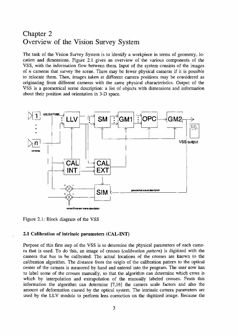
Chapter 2Overview of the Vision Survey System
The task of the Vision Survey System is to identify a workpiece in terms of geometry, location and dimensions. Figure 2.1 gives an overview of the various components of theVSS, with the information flow between them. Input of the system consists of the imagesof n cameras that survey the scene. There may be fewer physical cameras if it is possibleto relocate them. Then, images taken at different camera positions may be considered asoriginating from different cameras with the same physical characteristics. Output of theVSS is a geometrical scene description: a list of objects with dimensions and informationabout their position and orientation in 3-D space.
1
VSS output
cameras
~ CAL ~ CALf-----.--JINT f------7I EXT
1geome1rIcaI """"II dlIscrlptlon
Figure 2.1: Block diagram of the VSS
2.1 Calibration of intrinsic parameters (CAL-INT)
Purpose of this first step of the VSS is to determine the physical parameters of each camera that is used. To do this, an image of crosses (calibration pattern) is digitized with thecamera that has to be calibrated. The actual locations of the crosses are known to thecalibration algorithm. The distance from the origin of the calibration pattern to the opticalcenter of the camera is measured by hand and entered into the program. The user now hasto label some of the crosses manually, so that the algorithm can determine which cross iswhich by interpolation and extrapolation of the manually labeled crosses. From thisinformation the algorithm can determine [7,16] the camera scale factors and also theamount of deformation caused by the optical system. The intrinsic camera parameters areused by the LLV module to perform lens correction on the digitized image. Because the
3
current way of calibration requires a substantial amount of operator interaction, no exactprocessing times can be measured. An experienced user will perform the calibration of onecamera in approximately 60 seconds.
2.2 Calibration of extrinsic parameters (CAL-EXT)
The extrinsic calibration module is used to obtain extrinsic camera parameters, whichspecify position and orientation of the camera with respect to the absolute coordinatesystem. The higher level modules require this information for geometrical interpretation oftheir input data. At present extrinsic calibration is done by surveying a calibration object.The image of the calibration object, currently a 500x500x500 mm. cube, is digitized bythe camera under test. After this, the LLV module (discussed in the next paragraph)extracts lines at every contrast transition in the image. The user then selects and labels amaximum of nine visible lines corresponding to the cube's edges. In the future thisprocess will be automated. During this phase a world coordinate origin is identified (e.g.,one comer of the calibration object). The calibration algorithm, extensively described in[7], takes the intrinsic parameters and the set of calibration lines as its input and producesan extrinsic calibration file. The higher level modules use these data to recognize andmatch 3-dimensional objects from the 2-D LLV output. Extrinsic calibration currently alsorequires operator interaction, and will therefore take about 60 seconds to perform for eachnew camera location. The calculation of the parameters itself consumes less than onesecond of CPU-time.
2.3 Low-Level Vision (LLV)
The low-level vision is the main subjectof this thesis. Its task is to extract linesegments from the grey-level inputimage, which correspond to the objectedges in the image. An example of anworkpiece image is given in figure 2.2.Line extraction is a two-step process. Inthe first step, based on an algorithm designed by Lee [2,3,15,24], the image isfiltered by a one-dimensional convolutionfilter that amplifies the changes inbrightness along an image scan line. Thisoperation is performed in both horizontal·and vertical direction, yielding two sepa- Figure 2.2: Grey-level image of a workpiece
rate edge images. The edge image wherescanning is done in horizontal direction will contain edges of the vertically oriented lines,and vice versa. By employing an interpolation technique the exact location of the extreme(that corresponds to the location of the edge) can be calculated with subpixel accuracy.The edge detection algorithm takes about 6 seconds to completei.
iUsing a 32-bit compiler on a 80486-66MHz processor
4
In the next step, lines are fitted to the set of edge pixels. The algorithm, originally implemented by Broertjes [1,3,17], gathers a set of pixels of a straight line, and searches additional pixels for this set by fitting a line description to the set using a least-squares algorithm, and predicting an area where subsequent pixels may reside by extrapolating thefitted line. The line fitting is also done in two directions (i.e., horizontal and vertical). Theline segments are merged afterwards and one output file is produced. A number of parameters determine the performance of both low-level algorithms. It would be beneficial tofind out the optimal setting of these parameters automatically, independent of each specificscene. This is also an issue, investigated in this thesis. The line extraction algorithm runsfast when compared to the edge detection algorithm. The processing time is dependent onthe number of edgepixels but seldom exceeds 5 seconds.
Illumination proved to be one of the crucial aspects for the visibility of all edges of theobject(s) in the scene. With increased lighting however, the number of unwanted linesoriginating from cast shadows and unrevealed texture details also increases, so no easyrule can be formulated concerning illumination.
2.4 Structural matching (SM)
The structural matching module [4,5] takes the set of lines, generated by the LLV module,and the extrinsic calibration information as its input. Its task is to recognize subsets oflines that may constitute to (part of) an object. To this end, the matching algorithm alsohas at its disposition model descriptions of every basic subobject that may be present inthe workpiece. These models are described in a knowledge base as a series of predicatesthat define the properties of the lines in the subsets. With the extrinsic calibration information the structural matching module has a notion of which lines could be vertical,perpendicular, parallel, etc. The output of the structural matching consists of a number ofsubsets of the set of lines that are candidates for the edges of actual objects. There will bea number of false candidates depending on the strictness of the rules in the knowledgebase and the amount of noise lines from LLV. The balance between many false candidatesand possible missed candidates is again a matter of parameter setting. Processing time isnot only dependent on the number of input lines, but also on the structure of them. Arough approximation is about 1 second per matched object.
2.5 Geometrical matching (GMl/GM2)
At two stages of the VSS cycle, geometrical matching is performed. In the first stage(GMl) the individual object parts matched by the SM-module are handled. After this, the(now 3-dimensional) object descriptions are combined into more complete descriptions bythe OPC-module (discussed in the next section). The OPC output is fed into the GMmodule again to produce more accurate results.
The input of the geometrical matching module are subsets of lines that obey the knowledge base rules of a certain object. To determine if these lines could actually represent thisobject, the geometrical matching module employs an iterative projection algorithm. Aninitial 3-D object position, orientation and dimensions are (more or less randomly) chosen,and the "ideal" object model is projected into the 2-D camera image plane using theextrinsic calibration data. By minimization of the least-squares of differences between the
5
model lines and the input lines, the object position, orientation and dimensions are iteratively computed. Tjoa [6] showed that this algorithm converges to the optimal match (inalmost all cases) in a finite number of iterations. Typical iteration count is between 5 and20 iterations. A permissible restriction in the solution space is to expect that all objectshave one edge or plane in the ground plane (z=O). This improves speed and the ability ofthe algorithm to discard "impossible" objects (e.g., floating objects). Output of the GMmodule is a complete description of all recognized objects. This description is in theWorld Coordinate System, i.e., the camera position has been eliminated, and is thereforeirrelevant for the final result. The GM module performs the matching process at a speedof about 2 seconds per object.
2.6 Object part clustering (Ope)
The OPC module considers for every pair of subsets generated by the structural matchingmodule whether they belong to the same object. Due to occlusions, noise or objectdimensions, it may happen that more parts of the same object are recognized separately bythe SM module. Corresponding lines from the (partially) matched objects are checked forcolinearity with parametric allowable deviations. Using the extrinsic calibration information, subsets of lines originating from different cameras are also combined. Identical edgesviewed by multiple cameras improve accuracy during the next phase (GM). The algorithmcan also detect inconsistencies like objects that intersect each other. The output of theclustering process will provide a more condensed set of subsets, with more completeobject descriptions. The processing time required for clustering depends on the number ofinput objects but can be estimated to 10 seconds.
2.7 Synthetic image modeling (SIM)
The final method to verify correctness of the scene description is by image reconstruction.The Synthetic Image Modeling module recreates a grey level image from the scenedescription output by the GM module. To do this, it also needs to know the locations ofthe light source(s), the camera position (viewpoint) and the surface reflectance properties.A ray-tracing algorithm produces the grey level image. Although images can be createdfor any virtual viewpoint and/or lighting position (e.g., for manual verification), it is moremeaningful to choose the original camera and lighting positions. Ideally the differentialimage between the ray-traced image and the original digitized image should be zero. Iflarge areas with substantial difference occur, the output of the GM module could belabeled as "unreliable", or more advanced actions, as for instance automatic parameteradjustment, could be issued, followed by a re-run of the entire survey cycle. Korsten [8]describes the details of synthetic image modeling. One of the major issues of the renderingprocess is the choice of the correct reflection model (and parameters), and the presence ofhigher-order indirect illumination (illuminated surfaces that are light sources themselves),called interreflection. The actual ray-tracing process is very time consuming and thereforenot fit to incorporate in the system if high-speed performance is required. Reproducingsynthetic versions of all original input images may take at least several minutes with thecurrent available processing power.
6
2.8 Processing time discussion
As an example, the following list shows the expected processing time (in seconds) in caseof a VSS-survey performed with 4 cameras at 2 locations, thus producing 8 input images.Note that intrinsic calibration only needs to be performed once per camera.
When SIM is omitted, the time to complete one survey is about 17 minutes. With SIMincluded, the processing time exceeds 1Y2 hours. It is obvious that the parts that requirehuman interaction account for the largest execution times. Even faster hardware will notimprove the speed significantly (without SIM) if human interaction is not eliminated.Furthermore, there is no point in improving the performance of any module if there still isanother module with a much larger execution time (e.g., line extraction or SM versusextrinsic calibration).
7
Chapter 3Optimal Edge Detection
3.1 Introduction
The low-level vision module, briefly discussed in section 2.3, can be divided into severalsub-modules with different functionality. Each sub-module also represents a separatelyimplemented algorithm. The LLV-system is depicted in figure 3.1.
lenscorrection
edgedetection
lineextraction
post
processing
Intrinsiccamera parameters
Figure 3.1: Submodules within the LLV module
The lens-correction module theory is described in [16]. Note that it is the only module thatrequires the calibration information to correct the pixel locations for deviations caused bythe non-ideal optics of the cameras. If the new pixel locations are non-integer, thebrightness information is obtained from the neighboring pixels by bilinear interpolation.The lens correction improves accuracy during the geometrical matching phase. It alsoimproves performance of the line extraction module because edges of objects will appearas straight lines in the corrected image. The line extraction module will be the subject ofChapter 4. In the remainder of this chapter the edge detection method and improvementswill be discussed. The last submodule of the LLV, the postprocessing module, will bediscussed in Chapter 5.
3.2 Edge detection submodule
In this section a method is described to determine the location of edges by retrieving andcombining contrast information from different images taken from identical scenes undervarying lighting conditions. Edges are determined one-dimensionally, i.e., processing inhorizontal and vertical direction (called scan-direction) is done separately and yields twoedge-images. An image is said to contain an edge at a certain location if the course of thebrightness of an image (expressed as a pixel value) shows a discontinuity in the scandirection at that location. As an introduction a method is described to improve edge-detection on single images. After this, a method is described to obtain the edge images frommultiple input images, originating from different lighting conditions.
9
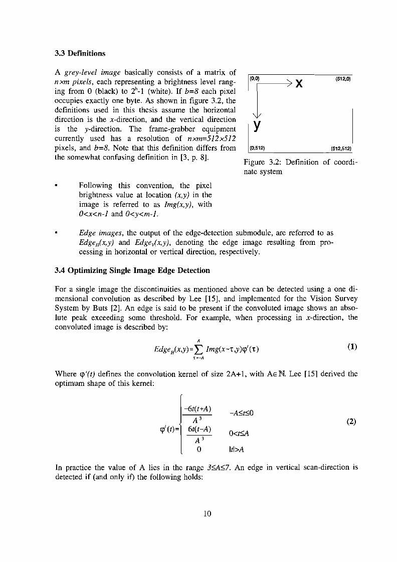
Figure 3.2: Definition of coordinate system
3.3 Definitions
A grey-level image basically consists of a matrix ofnxm pixels, each representing a brightness level ranging from 0 (black) to 2b-I (white). If b=8 each pixeloccupies exactly one byte. As shown in figure 3.2, thedefinitions used in this thesis assume the horizontaldirection is the x-direction, and the vertical directionis the y-direction. The frame-grabber equipmentcurrently used has a resolution of nxm=512x512pixels, and b=8. Note that this definition differs fromthe somewhat confusing definition in [3, p. 8].
• Following this convention, the pixelbrightness value at location (x,y) in theimage is referred to as Img(x, y) , withO<x<n-l and O<y<m-l.
(0,512)
(512,0)
(512,512)
• Edge images, the output of the edge-detection submodule, are referred to asEdgeH(x,y) and Edge jx,y) , denoting the edge image resulting from processing in horizontal or vertical direction, respectively.
3.4 Optimizing Single Image Edge Detection
For a single image the discontinuities as mentioned above can be detected using a one dimensional convolution as described by Lee [15], and implemented for the Vision SurveySystem by Buts [2]. An edge is said to be present if the convoluted image shows an absolute peak exceeding some threshold. For example, when processing in x-direction, theconvoluted image is described by:
A
EdgeH(x,y) =L Img(x-t,y)q>'(t)t=-A
(1)
Where <p'(t) defines the convolution kernel of size 2A+1, with AE N. Lee [15] derived theoptimum shape of this kernel:
-6t(t+A)-A~~O
A 3 (2)q>' (t)= 6t(t-A)
O<~A 3
0 Itl>A
In practice the value of A lies in the range 3~~7o An edge in vertical scan-direction isdetected if (and only if) the following holds:
10
!Edgev<x,y) I> IEdgev(x,y-l) I A 1Edgev<x,y) 1~IEdgev(x,y+ 1) I AIEdgev(x,y) I>Threshold
And similarly for the horizontal scan-direction:
IEdgeH(x,y) I> IEdgeH(x-1,y) I A IEdgeix,y)I~IEdgeH(x+1,y)1 AIEdgeix,y) I>Threshold
3.5 An adaptive threshold determination
(3)
(4)
A problem with the method described above is in the fixed threshold. The total number ofedgepixels found relies heavily on the threshold; a lower threshold increases the number ofedgepixels originating from noise in the image digitizing process or unwanted details suchas surface texture, whereas a higher threshold makes the poorly illuminated edges of thescene invisible. This also explains why each different scene requires a manual adjustmentof the threshold.
A solution to this problem is to divide the image in a number of regions (e.g., scan-lines)and adjust the threshold for each region until a satisfying number of edgepixels is found.This is identical to selecting the "best" edgepixels, i.e., those with the highest peaks. Unfortunately, one parameter is introduced while eliminating the other: how many pixels aresatisfying? The concept is undoubtedly better than the original; the threshold adapts to thenumber of edgepixels locally, and the results have proven to be less sensitive to variationsof the new parameter.
The new edge-detection algorithm is listed at the end of this chapter. Its primary input is aconvolved image, with peaks at locations with high contrast. The secondary input is theminimum desired number of edgepixels per region, called M. Output consists of twodestination images.
3.6 Edge detection using multiple images
The principle of extracting edges using multiple lighting configurations (see figures 3.33.5) is based on the idea, that a linear combination of two or more images still containsvalid information about the scene. Not necessarily will the sum of all images with different lighting conditions yield the image with the optimum illumination. Observe for
Figure 3.3: Test object, LC#1 Figure 3.4: Test object, LC#2 Figure 3.5: Test object, LC#3
11
instance the addition of the images in figure 3.4 and 3.5: the vertical edge in the center ofthe resulting image will become virtually invisible. Also in practice it is impossible torealize a physical illumination that is optimal for each region of the image. These facts ledto the idea of dividing all source images into m regions again, and optimizing the weightfactors for the linear combination of brightness information for each of these regionsseparately. This method is also known as photometric stereo [34,35,36]. This leads to twoseparate Sum images, one for each scan-direction, defined as:
where Imgi is one of n source images, Wid;,(X,y) is the weight factor for image i (l~i~n),
in direction dir that has to be determined for every region in every image, and gi,d;,(x,y) isthe average grey value of the region at (x,y) in image i. By subtracting the average greyvalue from the image, the chance of numerical overflow is minimized. The region size canbe chosen from any size larger than or equal to the convolution kernel size. If a one-dimensional region is chosen with a size equal to the size of the kernel (2A+1) the edge'speak-value can be expressed as:
A
Edgeix,y) = L SumH(x-1:,y)<p' (1:)'l'=-A
for horizontal scan-direction, and
A
EdgevCx,y) = L SumvCx,y-1:)<p' (1:)'l'=-A
for vertical scan-direction. The average grey value for image i is then defined as:
A
L Imgi(x-j,y)= j=-A
2A+1A
L Imgi(x,y-j)
( )j=-A
gi,v x,y = ~---2A+1
(6)
(7)
(8)
When both edge images have been calculated, optimal edge detection can be performedusing the algorithm discussed in section 3.5.
It is expected that the visibility of all 'real' edges (i.e., not those originating from noise)will be improved by the above scheme. Furthermore noise will decrease with an increasingnumber of images, because the noise across multiple images is not correlated, whereas theedge locations are strongly correlated. The weight-factors wi,dir can be chosen by deterrnin-
12
ing for each region in each input image:
-1 : light-dark transition0: no edge visible1: dark-light transition
If a brute force optimization-algorithm is used to determine optimum weight factors foreach region, 3R configurations have to be considered for each region.
13
3.7 Results
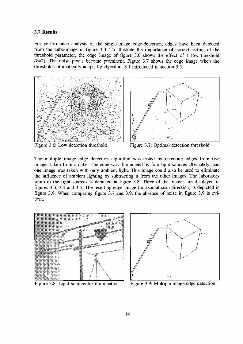
For performance analysis of the single-image edge-detection, edges have been detectedfrom the cube-image in figure 3.3. To illustrate the importance of correct setting of thethreshold parameter, the edge image of figure 3.6 shows the effect of a low threshold(0=2). The noise pixels become prominent. Figure 3.7 shows the edge image when thethreshold automatically adapts by algorithm 3.1 introduced in section 3.5.
The multiple image edge detection algorithm was tested by detecting edges from fiveimages taken from a cube. The cube was illuminated by four light sources alternately, andone image was taken with only ambient light. This image could also be used to eliminatethe influence of ambient lighting by subtracting it from the other images. The laboratorysetup of the light sources is depicted in figure 3.8. Three of the images are displayed infigures 3.3, 3.4 and 3.5. The resulting edge image (horizontal scan-direction) is depicted infigure 3.9. When comparing figure 3.7 and 3.9, the absence of noise in figure 3.9 is evident.
for each extreme in peaksize[] above thresholddo "store edge in destination image" od
]1 od
15
Chapter 4Line extraction
4.1 Introduction
The line extraction algorithm provides the first substantial data reduction of the VSS-input.The input image size is 256 Kbytes for a 512x512x8 pixelsxpixelsxbits image. An outputfile of the line extractor contains typically about 200 lines, occupying about 10 Kbytes.Lines are extracted from the horizontal edge image and from the vertical edge imageseparately. The resulting sets of lines are merged afterwards. An option would be to mergethe edge images first and extract lines from that image, but this idea was abandoned forthe following reasons:
• The horizontal edge image contains the edges obtained by scanning in thehorizontal direction. This means that the lines extracted from this imagewill be vertically oriented, that is, their angle l<pl with the horizontal axis islarger than 45°. The same holds conversely for the vertical edge image. Ifhorizontal(lvertical) lines appear in the horizontal(lvertical) edge image,they are more likely caused by noise and should therefore be discarded.
• A property of the used edge detector is that the edges that are detected areexactly one pixel thick, which makes uniform line fitting possible.Combining edge images would cover up this property.
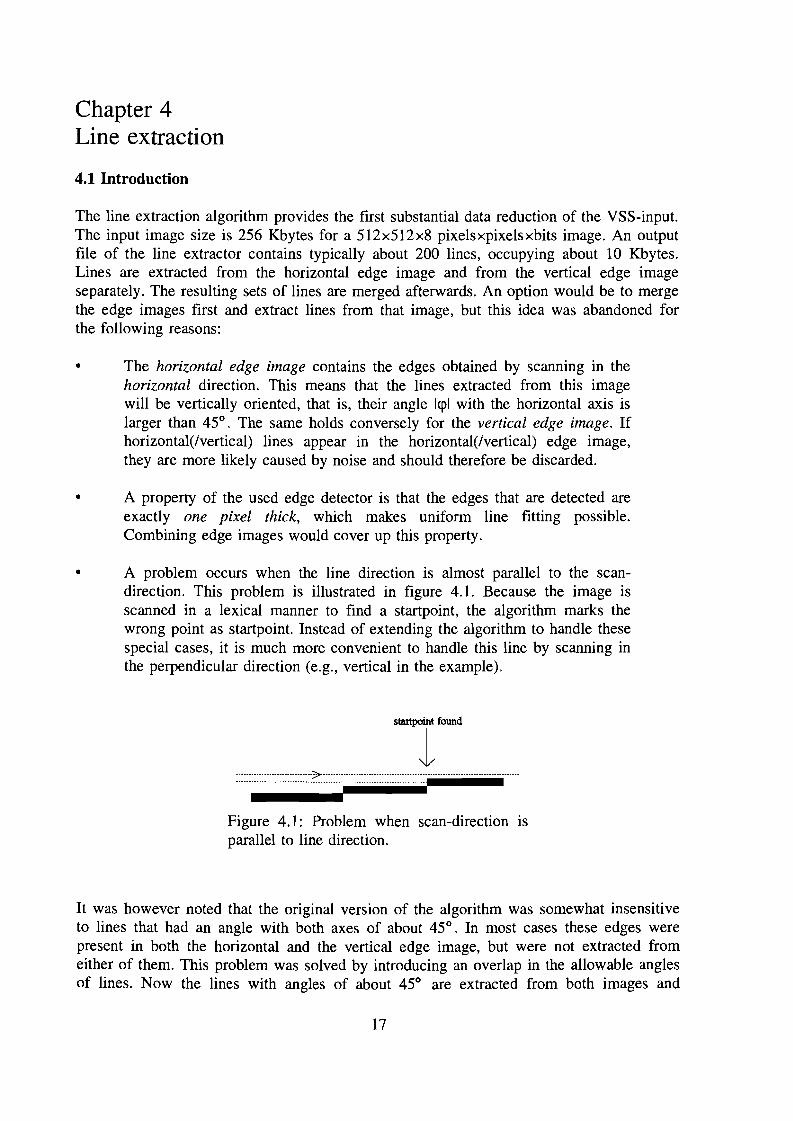
• A problem occurs when the line direction is almost parallel to the scandirection. This problem is illustrated in figure 4.1. Because the image isscanned in a lexical manner to find a startpoint, the algorithm marks thewrong point as startpoint. Instead of extending the algorithm to handle thesespecial cases, it is much more convenient to handle this line by scanning inthe perpendicular direction (e.g., vertical in the example).
..............................> .
Figure 4.1: Problem when scan-direction isparallel to line direction.
It was however noted that the original version of the algorithm was somewhat insensitiveto lines that had an angle with both axes of about 45°. In most cases these edges werepresent in both the horizontal and the vertical edge image, but were not extracted fromeither of them. This problem was solved by introducing an overlap in the allowable anglesof lines. Now the lines with angles of about 45° are extracted from both images and
17
merged into one line description during the post-processing phase (described in Chapter 5).
4.2 Line-extraction algorithm
As mentioned in the introduction, there are actually two line extraction algorithms, one foreach scan direction. Only one algorithm needs to be described here, as both algorithms arefunctionally the same, with only the coordinates swapped.
The mechanism to extract lines is to compose a set of edgepoints L that are more or lessaligned, and to add edgepoints to that set by predicting a region where subsequent edgepoints may be found. To obtain the first element of L, the edge-image is initially scannedfor an edgepixel, which will be marked as startpoint. The initial direction of the line willbe estimated by applying a predefined template. When no more edgepoints are found, thestart- and endpoint are projected on the least-squares fit of the line and stored. Theedgepoints of L are marked in a bitmap. This bitmap is a binary image that marks theused edgepoints so that they cannot be selected as a new startpoint.
Algorithm 4.1: Line extractor
Abbreviations used:
s=startpointp=predicted pointe=endpoint
s=(O,O)while found next point s not in bitmapdo
L={s}<p=initial-dir(s)e=sdo
predict position p on next scan line from e and <pfound ~ look for new endpoint e near p in region: [search-width,maxgap]if found
L=Luemark e in bitmap<p=leasts-squares-dir(L)
fiod while foundproject sand e perpendicular on the line defined by Lif Is-el>min-length and IL(<p,scan-direction)l>rrl8 ~ store s,e fi
od
18
4.3 Algorithm detailsSome actions defined in the algorithm above need elucidation and will be described below.
4.3.1 Initial search direction estimation
The initial direction that is estimated after the startpoint has been found is derived bymultiplying the pixelvalues that lie around s with the elements of different 5x5 templates.The template that yields the highest sum of products has highest correlation with theactual line direction and identifies the line direction with an error of at most 1t/8. Whenscanning is done lexically in the horizontal direction, four templates To-. Tj suffice, withangles ranging from 0 to -31t/4. This is illustrated in fig. 4.2.If s=(xs'Y) for every template t, the sum
• j-2 -1 0 1 2
-2
-1
o12
0 0 0 0 00 0 0 1 10 0 0 2 20 0 0 1 10 0 0 0 0q>=O
0 0 0 0 00 0 0 0 00 0 0 1 00 0 1 2 10 0 0 1 2
q>=-rc/4
0 0 0 0 00 0 0 0 00 0 0 0 00 1 2 1 00 1 2 1 0
q>=-rc/2
0 0 0 0 00 0 0 0 00 1 0 0 01 2 1 0 02 1 0 0 0
q>=-3rc/4
Figure 4.2: Templates for initial direction estimation
2 2
S(t) = L L Tt(iJ)Edge(xs+i,ys+])i=-2 j=-2
is calculated. The initial direction is <p=-m1t/4, where
m : S(m)=max[S(t)ll~t~4]
4.3.2 Prediction of next edgepixel position
(9)
(10)
If the scan direction is horizontal, and the last edgepixel found is e=(xe,Ye)' the coordinatesof the i-th edgepixel pi=(xii),Yli)), i scan-lines below e can be predicted as
x (z)=x +i· tan(<p +~), Yp(l)=ye+ip e 2
(11)
with O<i'5.max-gap. This introduces a line extraction parameter max-gap. With this parameter the maximum look-ahead of the edgepixel predictor can be specified, in case of a'gap' in the line. While small values of this parameter enable the line extractor tosuccessfully track a line with small interruptions caused by noise, larger values introduce
19
I ISearch Width
~ )'rediCtiOD
--- i"{ IMax. gap! 1\ •I I"i i
the danger of separate lines that will be detected as one single line. Large values of maxgap may also cause many single noise pixels to form more or less 'random' lines.
4.3.3 Search for an edgepixel nearby a predicted point
When no edgepixel is found at the predictedposition, the search will be extended in thevicinity of this position, according to the search-width parameter. This parameter determines the maximum deviation from the predicted position that an edgepixel may have. Ifsearch-width=3 for instance, 7 locations onthe scan-line of the predicted location areconsidered. If none of these locations containan edgepixel, the search is repeated at thenext prediction on the next scan-line. Thevalue of search-width determines the amount Figure 4.3: Search environmentof deviation that is allowable for the edge-fol-lowing process. Small disturbances are likely to occur and these will be resolved becauseof this parameter. Larger values of search-width may cause the line direction to becomeless accurate because too many false edgepixels are included in L.
4.3.4 Least-squares line estimation
The purpose of the least-squares line estimation is to find the parameters a,b, and c for theequation ax+by+c=O to describe the best fitting line through the points in L. This is doneby minimizing the sum
n
LSE=L (GXi+byi+cii=l
(12)
If all elements (Xj,y)E L, O<i~n are exactly aligned, LSE=O (perfect fit). The derivation ofthe optimum values for a,b, and c is described in [3] and [18] and will be repeated below.First, a number of sums is defined.
Sy=LYj' S.u=I:xj2
,j=! j=!
n n n n
S =~y2yy L j'
j=!
n
(13)
Further define the symmetric matrix
n
S=I: vjv/j=!
as the scatter matrix of the n given points.
(14)
20
The first step [18], is to standardize the points by subtracting the mean of the set fromeach point. The standardized scatter matrix 8' of the set of standardized points is:
(15)
The second step is to find the principal eigenvector of the standardized scatter matrix 8'.The best line estimation is the unique line through the mean of the set of points andparallel to this eigenvector. The eigenvalues of the standardized scatter matrix 8' are asfollows:
(16)
where
(17)
Under the assumption that 8'12*0 The principal eigenvector is now as follows:
(18)
Special cases occur when 8'12=0. In this case the line is either vertical (S'Il<S'22 -7
a=l,b=O) or horizontal (S'Il';?S'22 -7 a=O,b=l). Now a and b are estimated, c can beestimated by using the line equation ax+by+c=O and by filling in for x and y the meanvalues of coordinates of the set of points (Sin and Sin respectively):
c= aSx +bSyn
(19)
The line angle <p is calculated from a and b by one of two formulas, for numerical stability. If both lal and Ibl are very small, the line direction cannot be resolved.
4.3.5 Perpendicular projection
(Ia 1< Ibl)
(lal~lbj)
(20)
The projection (x',y') of a point (x,y) on the line specified by a,b, and c is calculated bythe following formulas:
21
(21)
When compared to [3], the formulas have been modified to guarantee numerical stability.
4.4 Performance analysis
4.4.1 Parameter setting
The behavior of the current line extraction algorithm is in the current implementationdetermined by three parameters: max-gap, search-width and min-length. Their meaninghas already been described. The previous version, implemented by Broertjes [3] had muchmore parameters. This was useful in the development stage to investigate whichparameters were important for the line quality, but in the current implementation allparameters that do not significantly influence the performance of the algorithm have beenabandoned. Setting fixed values for the above parameters cannot be justified. Their settingdetermines the final result. Automatically determining the optimum setting of eachparameter is a difficult task. Two different approaches can be distinguished:
1. Extracting properties from the edge-image, such as counting noise pixels ortotal pixels, and presetting the parameters based on earlier findings.
2. Iteratively adjusting the parameters by evaluating the line extraction result,for instance by judging the number of lines or the average line length.
No clear relationship was found between the edge image and the optimal parametersetting, so no rules can be specified to use the first approach. The second approachconsumes a huge amount of CPU-time, and is therefore undesirable. However, in thecurrent implementation the operator adjusts the parameters manually, following the secondapproach in an intuitive way. It would be possible to optimize the number of extractedlines to a value not exceeding a certain upper limit by increasing the min-length parameter, for instance. The other two parameters determine the accuracy of the result. The maxgap parameter can be decreased to a small value if the post-processing algorithm takesover this task. The search-width parameter should be kept small if the image contrast ishigh, but should be increased if it is known a-priori that the workpiece edges are not100% straight.
4.4.2 Line extraction accuracy
The accuracy of the line extraction is influenced by a number of imperfections in the VSS.These imperfections can be modeled as noise sources. The extracted lines inherit a numberof these errors in the trajectory from the optical system up to the line coordinatescalculation. The following errors can be distinguished:
(1) Physical defects in the workpiece(2) Imperfection of the optical system of the camera(3) Quantizing noise/error of the CCD (blooming)
22
(4) Analog noise in the cables(5) Quantizing noise/error of the frame-grabber(6) Calibration errors, resulting in lens correction errors.(7) Edge detection errors, caused by (1..6) and numerical resolution(8) Line extraction errors, caused by incorporating noise pixels in the LSE estimation(9) Geometrical matching errors, caused by the above errors and errors in model-to
workpiece relation.
If an overall accuracy measurement is made, all these errors contribute to the overall error.Measurement of a 500x500x500 rnm. cube showed repeatedly that the overall geometricalmatching error is within 1% (5 rnm.) of the actual workpiece dimension. This is asufficiently low error to ensure correct functioning of the local sensors of the finalintegrated welding system.
It is hard to measure the individual magnitude of the errors. Broertjes [3] performed ameasurement of the errors caused by (7) and (8) by applying a synthetic image. He foundan average deviation of ±O.5 pixel, using subpixel accuracy. This result may not beaccurate due to rounding errors in the raytracer that produced the picture, so no validconclusions may be drawn from this result.
If the system is fully operational, it would be worthwhile to investigate the increase in theoverall error, if subpixel accuracy is abandoned. This would increase the error, caused by(7), but it is expected that these errors are systematic and are cancelled out by the leastsquares line-estimation. If the error is acceptable, the use of integer arithmetic could savesome valuable CPU-time.
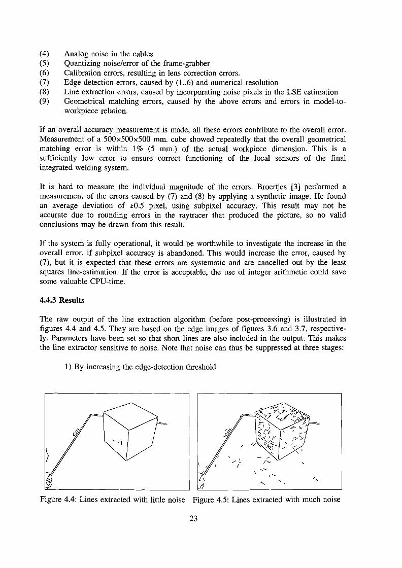
4.4.3 Results
The raw output of the line extraction algorithm (before post-processing) is illustrated infigures 4.4 and 4.5. They are based on the edge images of figures 3.6 and 3.7, respectively. Parameters have been set so that short lines are also included in the output. This makesthe line extractor sensitive to noise. Note that noise can thus be suppressed at three stages:
1) By increasing the edge-detection threshold
,I
/,
J , .......\
Figure 4.4: Lines extracted with little noise Figure 4.5: Lines extracted with much noise
23
2) By increasing the minimum line-length during line extraction3) By increasing the minimum line-length during post-processing
Properly selecting the stage to suppress the noise implies choosing between some contradicting interests. Edge detection noise influences line extraction accuracy but increasesedge visibility. A good choice is to discard short lines during the post-processing phase (3)rather than during the line extraction phase (2).
4.4.4 Gradient information
If the sign of the convolution result during edgedetection is preserved, the averagemagnitude of the edgepixels that constitute a line contains information on the imagegradient in the direction perpendicular to the line. This information can be provided asadditional information with the lines. This feature however is not supported by theknowledge bases of the structural matching module. The output of gradient information isdiscontinued in the current implementation, but could easily be restored in the future, ifthe gradient information proves to be useful.
By averaging the luminance of a surface and taking into account the reflectance propertiesof the material and the light source position, surface normals can be estimated. This couldbe a useful feature to be examined in the future.
24
--- Line segment;......··....···........1Lin~ segment......................... EnVironment
Chapter 5Post-processing algorithm
5.1 Purpose of post-processing
The set of lines generated by the line extraction algorithm can be processed to overcomeseveral limitations of the line extraction algorithm itself. To this end, the set of lines isprocessed by an algorithm that detects if lines are colinear or parallel within certainallowable deviations. If they are, both lines are merged into one line by fitting a leastsquares description to the original line parameters. The length of the lines is used as aweight factor, so that short (noise) lines can influence the location of larger lines onlyslightly. The algorithm, called CONNECT, was first implemented by Kaptein [4].
5.2 Automatic post-processing
The criterion upon which is decided if two lines are merged is determined by a number ofparameters. A rectangle (line segment environment) is defined around each line, with thedistance from the line endpoints to the rectangle parametrized (wl,wd, see figure 5.1). Thefirst condition that has to be met is that the rectangles of two lines intersect. In figure 5.1,this is the case for the line pairs (1,2) and (2,3). The second condition that has to be metis that the difference in the angles of the lines does not exceed some maximum. Thismaximum angle is a parameter conveniently called 'max-angle'. For every pair in the set,the above two criteria are tested. The resulting reduced set may contain new candidatepairs for merging, so the algorithm is applied recursively to this set until no furtherreductions can be made. All lines in the final set that are shorter than min-line-Iength arediscarded.
../~::~>...../ ..~::~:.; ....//
......••.. . .
..•....•.
l.. L~ i wd
Figure 5.1: Connect 'cases'
25
The new line parameters of two merged lines are calculated as follows.
2. The sums defined in (13) in section 4.3.4. are now calculated as:
s= 111 1(xlb+xle) + Ilzi (x2b+x2e)x
S = Illl(ylb+yle) + Ilzl(y2b+y2e)y
S = III I(xI;+xIJ + Ilzl(x2;+x2J.xt (22)
s = III I(y1;+yIJ + Ilzl (y2;+y2;)yy
s = III I(xlb ylb + xleyle) + Ilzl(x2b y2b + x2e y2e)xy
n= 2111 I+211z1
3. The resulting line parameters a,b, and c are calculated in the same way as duringline extraction using formulas (14) to (19) from section 4.3.4.
4. From the set ((xlb,y1b)' (xle,yl), (x2/J>y2b), (x2e,y2e)}, the two points furthest apartare selected as new start- and endpoints. They are perpendicularly projected on themerged line using (13) from section 4.3.4.
Properties of the CONNECT algorithm are:
•
•
•
Short lines that are not merged with adjacent lines toform longer lines can be rejected. This provides anadditional way of noise suppression.
Parallel lines extracted from different edge images(i.e., different scan-directions) will be averaged intoone line that is more accurate.
Line gaps that were 'too big' for the line extractionalgorithm can be safely detected by the CONNECTalgorithm, because the direction of both line segments is known, which was not so during lineextraction. If the maximum-gap parameter is set toobig during line extraction, a problem occurs whenlines in other directions are nearby. This problem isillustrated in figure 5.2.
Edges:
Extracted lines:
Figure 5.2: Skipping wrong'gaps' during line extraction
• A drawback of CONNECT is that the line accuracy actually decreases whenadjacent lines not corresponding to the same object edges are merged. This can beprevented by setting the parameters more strict (smaller).
26
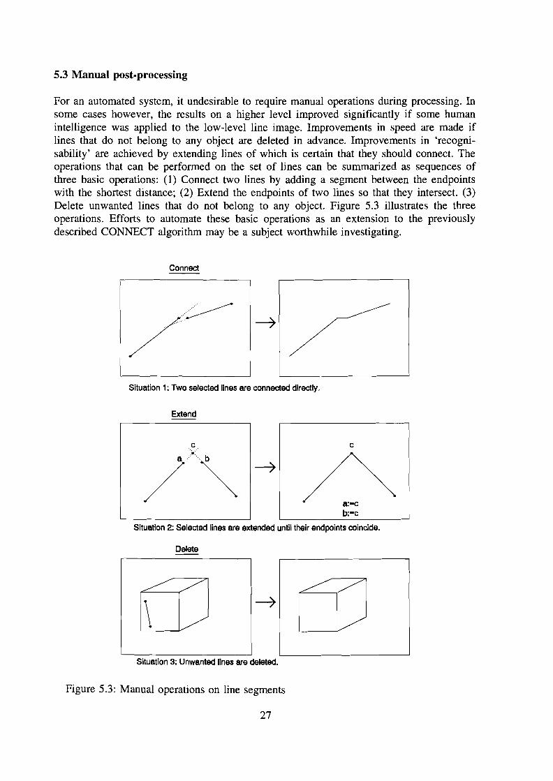
5.3 Manual post-processing
For an automated system, it undesirable to require manual operations during processing. Insome cases however, the results on a higher level improved significantly if some humanintelligence was applied to the low-level line image. Improvements in speed are made iflines that do not belong to any object are deleted in advance. Improvements in 'recognisability' are achieved by extending lines of which is certain that they should connect. Theoperations that can be performed on the set of lines can be summarized as sequences ofthree basic operations: (1) Connect two lines by adding a segment between the endpointswith the shortest distance; (2) Extend the endpoints of two lines so that they intersect. (3)Delete unwanted lines that do not belong to any object. Figure 5.3 illustrates the threeoperations. Efforts to automate these basic operations as an extension to the previouslydescribed CONNECT algorithm may be a subject worthwhile investigating.
Connect
Situation 1: Two selected lines are connected directly.
Extend
c c
a:-cb:""c
Situation 2: Selected lines are extended until their endpoints coincide.
Delete
\Situation 3: Unwanted lines are deleted.
Figure 5.3: Manual operations on line segments
27
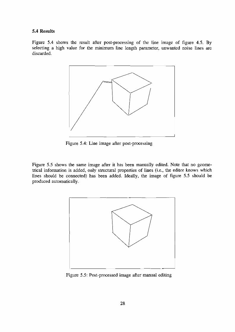
5.4 Results
Figure 5.4 shows the result after post-processing of the line image of figure 4.5. Byselecting a high value for the minimum line length parameter, unwanted noise lines arediscarded.
Figure 5.4: Line image after post-processing
Figure 5.5 shows the same image after it has been manually edited. Note that no geometrical information is added, only structural properties of lines (i.e., the editor knows whichlines should be connected) has been added. Ideally, the image of figure 5.5 should beproduced automatically.
Figure 5.5: Post-processed image after manual editing
28
Chapter 6Implementation of a User Interface
6.1 Introduction
The Vision Survey System that is developed by the Measurement and Control section ofthe department of Electrical Engineering is a complex software product. This means that itconsists of multiple functionalities, multiple source files and multiple executables.Furthermore the system is developed by a team of programmers that have to build on whattheir predecessors have left behind. This poses severe considerations on the softwaredevelopment. The programmer must conform to certain layout and documentation rules inorder to make his sourcecode accessible to future programmers. These rules have beensummarized in the 'C-Guidelines' document by W. H. A. Hendrix. [12]
Apart from this 'programming etiquette' the large software system that is emerging callsfor an environment that is suitable for integrating the various components. Up to now,every programmer designed his own user-interface for embedding his part of the VSS.This may cause problems when the entire VSS system should be operated in the future:Each block of the VSS requires its own specialist operator to execute. The proposedenvironment should overcome this problem and make individual user-interfaces obsolete.To accomplish this, it should meet the following requirements:
1. It should present an understandable user-interface, which allows a novice tooperate the entire Vision Survey System without difficulty.
2. It should introduce consistency of operation throughout all blocks of thesystem.
3. It should have graphical capabilities to allow the user to monitor the resultsof the various VSS-functions. (I.e., line drawing, displaying of bitmaps).
4. It should offer easy parameter editing in a consistent way for all functionalities of the VSS.
5. It should be able to deal with large amounts of data and not run out ofmemory at any time.
6. It should be designed so that future extensions and/or updates of the VSScan be added without much effort.
The MS-Windows environment was selected as a logical candidate for a user-interface forthe following reasons:
• It avoids the need for the programmer to worry about graphics modes, menulayouts, screen resolutions etc. This is all handled by Windows itself.
29
• Windows environments in general have proved to be intuitively understandable and easy to operate.
• MS-Windows will continue to have a large impact in the PC-world; it is anaccepted standard.
Developing applications for Windows however is not trivial and requires thoroughunderstanding of all its internal mechanisms by the programmer. But this should not be aburden for any VSS programmer. There should be a separation of concerns between thedeveloper of the user-interface and the VSS-programmers. While the former simplyintegrates a number of black boxes, the latter should be able to design them with onlyminimal limitations to what his black box should look like. This concept should be kept inmind at all times to make the user-interface successful. One cannot expect every VSSprogrammer to get familiar with windows programming.
The following part of this document describes the first attempt to design an MS-Windowsapplication that will meet the requirements mentioned above. This design should by nomeans be considered complete. Also the time lacked to ensure that the currentimplementation is correct (in terms of coding errors and following conventions). This iswhy a dedicated programmer should take over this task. The rest of this document issimply a summary of the findings and exploration of the MS-Windows system, whichappeared to be an immense system in which there seems to be a provision for just abouteverything one would expect an interface to do.
file ~alibrate!:lV ~tructM §eoM .QPC
\\/
Figure 6.1: VSS User-Interface main window
30
6.2 Integrating programs in a Windows environment
Various approaches can be devised to integrate a large number of independent componentsinto a whole. The following aspects should be considered:
Is it desirable to integrate all functions into one executable, together withthe windows functions? The alternative is to let windows call the variousexecutables and only display the results of a VSS function. (Spawn method).
How should the data communication take place? Up to now, the communication was entirely via files. This proves to be a safe and stablemethod. However, avoiding the saving and reloading of multiple greyscaleimages (256K each) could be a significant speed improvement.
The VSS system could be implemented as a series of separate processesthat operate independently in the Windows multi-tasking environment. MSWindows offers a 'Dynamic Data Exchange' mechanism (DDE) to facilitatethe exchange of data objects. If this would seem too complex, a simplerscheme (i.e., single task) must be devised.
What limitations are posed on the deliverants of the individual VSS blocks?Clearly, their code should run silently without any printf statements andshould obey the ANSI-C standard, for instance. How will a block report anyerrors or send messages to the UI? For example, each block could exit withsome error code, which should be interpreted by the UI. Can the use of anyWindows statements in the blocks be avoided? Windows requires differentstatements for memory allocation, file handling etc. Ordinary fopen () andmalloe () statements must be translated.
Programming Windows is a matter of following a large amount of conventions and a greatdeal of object-oriented thinking. Good reference material and lots of examples are anecessity. "Programming Windows 3.1" by Charles Petzold [9] is one of the beststarting points. Also the Windows ADK section of MetaWare's HIGH-C manual isimportant, because there are some exceptions in coupling 32-bit applications to the 16-bitWindows environment. Although the VSS applications may call for 32-bit environmentbased compilers, there are several options for the user interface itself. HIGH-C has somenotorious bugs in release 3.11 regarding the Windows development part. Other compilersthat have proven to be very suitable are: Borland C/C++ vn. 3.1 and 4.0, and the latestMicrosoft C compiler.
31
6.3 Windows principles and conventions
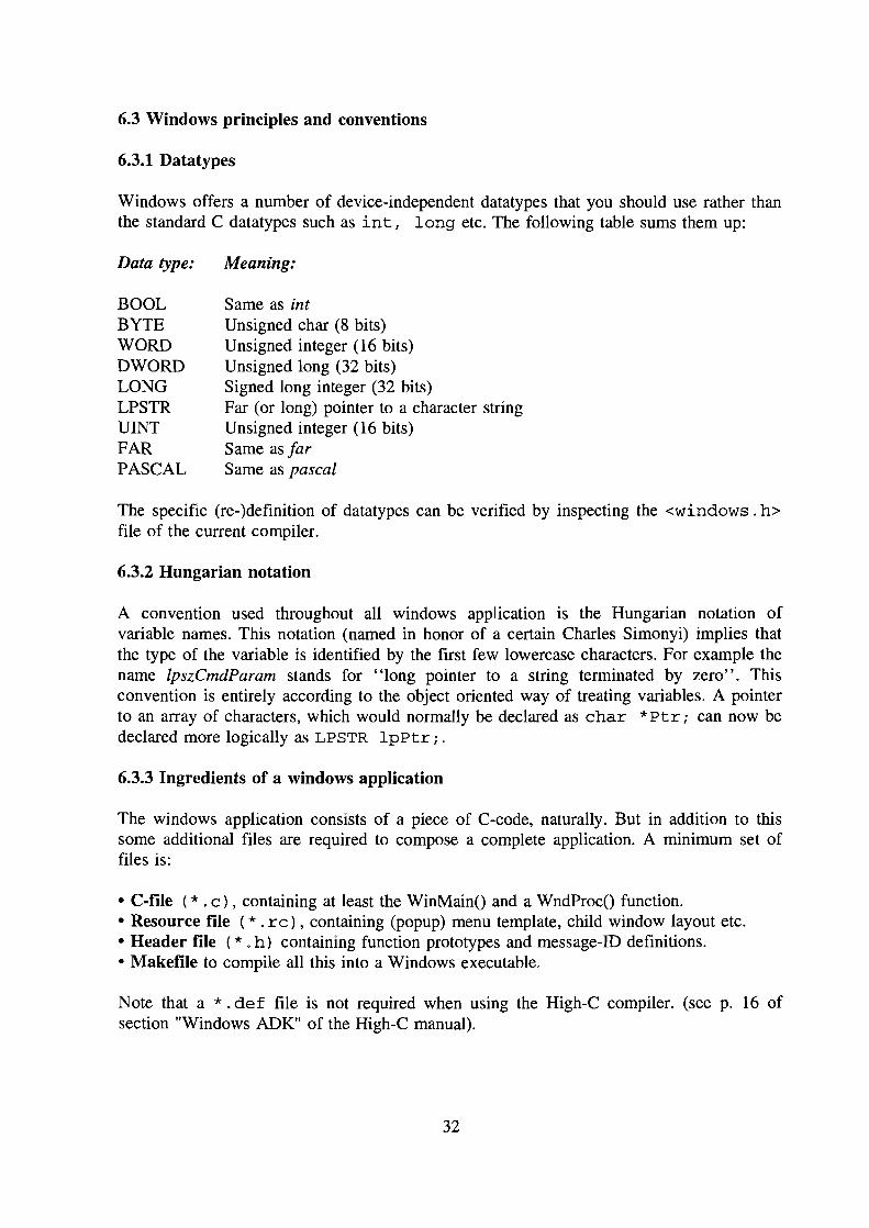
6.3.1 Datatypes
Windows offers a number of device-independent datatypes that you should use rather thanthe standard C datatypes such as int I long etc. The following table sums them up:
Data type:
BOOLBYTEWORDDWORDLONGLPSTRUINTFARPASCAL
Meaning:
Same as intUnsigned char (8 bits)Unsigned integer (16 bits)Unsigned long (32 bits)Signed long integer (32 bits)Far (or long) pointer to a character stringUnsigned integer (16 bits)Same as farSame as pascal
The specific (re-)definition of datatypes can be verified by inspecting the <windows. h>file of the current compiler.
6.3.2 Hungarian notation
A convention used throughout all windows application is the Hungarian notation ofvariable names. This notation (named in honor of a certain Charles Simonyi) implies thatthe type of the variable is identified by the first few lowercase characters. For example thename lpszCmdParam stands for "long pointer to a string terminated by zero". Thisconvention is entirely according to the object oriented way of treating variables. A pointerto an array of characters, which would normally be declared as char *ptr; can now bedeclared more logically as LPSTR lpPtr;.
6.3.3 Ingredients of a windows application
The windows application consists of a piece of C-code, naturally. But in addition to thissome additional files are required to compose a complete application. A minimum set offiles is:
• C-file (*. c) , containing at least the WinMainO and a WndProcO function.• Resource file (*. rc) , containing (popup) menu template, child window layout etc.• Header file (*. h) containing function prototypes and message-ID definitions.• Makefile to compile all this into a Windows executable.
Note that a *. def file is not required when using the High-C compiler. (see p. 16 ofsection "Windows ADK" of the High-C manual).
32
6.4 The user-interface source code
6.4.1 Principle of operation of a Windows program
A window is an object. It has to be created before it exists. These steps are performedupon booting a windows application (i.e., by double clicking its icon). The applicationentry point is always WinMain ( ) , just as main () is the entry of an ordinary C program.The window of your application is based on a so-called window-class. In this windowclass some characteristics of all windows based on this class are defined. The mostimportant characteristic of the window-class is the identification of the window procedure.This is the C function that handles the messages that the window is going to send whenthe user selects menu options, resizes the window, etc. This function is called by theWindows operating system; it is therefore often referred to as the window's callbackfunction.
After-the window-class is registered (using the RegisterClass () function) the actualwindow must be created. This is done with the CreateWindow () function. If multipleinstances of the same application are booted, they can all be based on the same windowclass. This is why the window-class registering should be done only once (on the firstinstance of the application), while each of possibly multiple instances of the applicationare identified by their hIns tance value.
When the application window is created, it is displayed using the ShowWindow () andthe UpdateWindow () functions. After this, wndMain () enters its message loop, andthe various messages it receives are dispatched to the WndProc () function. The windowspseudo-multitasking is non-preemptive. Task switches are accomplished by switchingbetween various message loops.
6.4.2 WinMain () function
The structure of the WndMain () function is similar for most applications. All Windowsfunctions use the PASCAL calling convention because it's more efficient (fast) than thedefault C calling convention.
#include <windows.h>#include <menu.h>
HANDLE hInst;
int PASCAL WinMain(HANDLE hInstance,HANDLE hPrevInstance,LPSTR IpCmdLine,int nCmdShow)
{static charHWNDMSGWNDCLASS
szAppName [] == "VSS" ;hWnd;msg;WndClass;
33
1*1*
Register main window class if this is thefirst instance of the app.
A couple of references outside the WinMain () function are defined in the registeringphase. The contents of the menubar that will be displayed at the top row of the window
34
are specified with:
WndClass.lpszMenuName = "MenuMenu"
The shape of the icon is identified with:
WndClass.hlcon = Loadlcon (hlnstance, "menu");
Both "MenuMenu" and "menu" refer to entries in the resource file. A possible layout of(part of) the resource file could be:
1* FILE: menu.rc *1
#include <windows.h>#include "menu.h"
menu ICON menu.ico
AboutBox DIALOG 52, 57, 144, 55STYLE DS_MODALFRAME I WS_CAPTION I WS_SYSMENU{
MENUITEM "Edi t " ,MENUITEM SEPARATORMENUITEM "RUN LLV",
}
II ... other popup menu's ...
} 1* end MenuMenu *1
VIEW_H_EDGESVIEW_V_EDGES
VIEW_LINESVIEW_CONNECT
EDIT_LINES, GRAYED
Let it be noted that this resource file is not necessarily representative for the menustructure of the final user-interface. It is meant as an example. After each menu item inthe "MenuMenu" template, there is a number identifying the item. These numbers aretypically identified in the * .h file as follows:
#define IDM_NEWSCENE 123
The number '123' is completely trivial, as long as it is unique. This is the numberWindows will send to the WndProC () when you click on this menu item with themouse. WndProc () has to handle the action associated to this number. The name that isused in both the resource file and the C file is prefixed by 'IDM_' (for ID-Message) byconvention.
6.4.4 WndProc () function
The WndProc () function is called whenever a message is available in the messagequeue. The programmer need not to worry when the messages will be sent. He only needsto recognize the messages he wants to support, and return 0 if a message could beprocessed successfully. All messages that cannot be processed by wndProc () must betransferred to Defaul tWndProc ( ) ; WndProc () can even send a message to 'itselfwhile handling a message in WndProc ( ) . This was done in the user 'IDM_EXIT' option.
Several types of messages can be distinguished. Upon entry the message parametercontains the number of the message. Examples of messages are WM_CREATE, which issent only once right after the window is created. The application can do its initializationsthere. In contrast to this is the WM_DESTROY message, which terminates execution ofthe application. The most important messages to the application are without doubt theWM_COMMAND and WM_PAINT messages. The messages are most convenientlyparsed with a swi tch (message) statement. The unsupported messages are not includedas cases and they are automatically sent to DefWindowProc ( ) ;. When a user selects amenu item, a WM_COMMAND message is send to wndProc (). The wparamparameter now contains the message number as it was defined in the *. h file. A secondary switch (wparam) statement can parse the specific user commands. All this couldbe done in a separate function, e.g., HandleUserCommand ( ), as was done in the
36
following example.
long FAR PASCAL MenuWndProc (HWND hWnd,WORD message,WORD wParam,LONG lParam){
switch (message){
case WM_CREATE:/* Perform initialisations */return 0;
case WM_COMMAND:/* If an unknown WM_COMMAND is encountered, thedefault window proc must be called */if(HandleUserCommand(hWnd,message,wParam,lParam))break;else return 0;
case WM_SIZE:if (lParam) InvalidateRect (hWnd, NULL, TRUE);return 0;
case WM_PAINT:/*If there is nothing to repaint the defaultwindow proc must be called */if (HandleRepaint(hWnd)) break;else return 0;
Note that break; statements are obsolete (unreachable code) if a return 0; is inplace. There is one extra function call here that will be described in a following section:the HandleRepaint () function that is called upon receipt of a WM_PAINT message.This message is generated whenever a window is resized, exposed, maximized, etc.Generally a WM_PAINT will be sent whenever Windows 'thinks' that the windowsgraphical area (called the client area) contents have become invalid. If the applicationhandles a WM_PAINT message at all times, this ensures that the window contents willreflect the correct information in all cases.
The following code fragment handles user commands, that is, some menu item selections:
long FAR PASCAL HandleUserCommand
37
(HWND hWnd,WORD message, WORD wParam,LONG IParam){FARPROC IpProc;
switch (wParam){
case IDM_EXIT:DestroyWindow (hWnd);return 0;
case IDM_ABOUT:IpProc = MakeProclnstance (About, hlnst);DialogBox (hlnst,"AboutBox",hWnd,lpProc);FreeProclnstance (lpProc);return 0;
case IDM_DRAWLINES:II this is a user-defined globalPaintMode=DRAWLINES;II Force a WM_REPAINTInvalidateRect(hWnd, NULL, TRUE);return 0;
case IDM_EDGEDETECT:PaintMode=EDGEDETECT;InvalidateRect(hWnd,NULL,TRUE);return 0;
II other case ... : statements ...
} 1* end switch(wParam); *1
1* This function could not handle the user command, so the* default window procedure MUST take care of it.* This is signalled by returning a nonzero value.*1
return 1;}
It should be noted that not all message numbers as they appear in the resource scriptabove are handled by this function. The object was simply to give an idea of how thesemessages should be handled. It is generally not a good idea to put whole chunks of codein here. Probably the simplest way is to call some function in each case.
38
6.5 Repainting the client area
6.5.1 Handling the WM_PAINT command
There are various possible schemes for repainting the client area. The scheme that will bepresented here assumes that the client area contents depend on the menu item that wasmost recently selected. (i.e. when a line drawing from menu A is displayed, and thescreen is resized, the line drawing should be re-displayed rather than some bitmap imagefrom menu B). This can be accomplished by storing the most recently selected menuIDnumber into a global variable indicating the paintmode:
int PaintMode=O;
A value of zero indicates that no repainting needs to be done. For example, in case of aIDM_DRAWLINES message, the only actions that have to be taken is to store thatmessagenumber in the paintmode and then mark the client area as invalid. Windows willrespond with a successive WM_PAINT message. Recall the following fragment from theHandleUserCorrunand ( ) function:
case IDM_DRAWLINES:PaintMode=DRAWLINES;InvalidateRect(hWnd, NULL, TRUE);return 0;
The WM_PAINT message handler calls the following function:
long FAR PASCAL HandleRepaint(HWND hWnd){
switch (paintMode){
case DRAWLINES: HandlePaintLines(hWnd); return 0;case EDGEDETECT: HandlePaintEdges(hWnd); return 0;
}return 1;}
Which in turn calls the proper HandlePaint ... () function.
6.5.2 Drawing graphics in the client area
For simple graphics like lines, MS-Windows offers the well-known MoveTo () andLineTo () functions. Before they can be used however, some preparations must be doneso that Windows knows which coordinate system to use, for instance. First of all, whenhandling a WM_PAINT message all graphical actions onto the client area must beembraced by the BeginPaint () and EndPaint () functions. This is to prevent otherprocesses from interfering with the client area. The Beginpaint () function alsosupplies a handle to the device context (type HDC). The HDC concept is described invarious reference manuals, so it will merely be presented here.
The following code fragment defines a coordinate mapping of 512x512 pixels, regardless
39
of the size or aspect ratio of the client area. Then an ASCII file containing coordinates oflines is opened and scanned. The lines are drawn in the client area and the function exits.The file format of the input file is described in appendix C.s
This routine uses standard C file handling functions. Although Windows manualsdiscourage this, it seems to work fine. Note that in the current implementation this simpleapproach of reloading the data every time has been abandoned. Instead, the line image isloaded into a datastructure only once.
6.5.3 Displaying bitmaps in the client area
The displaying of bitmaps can be accomplished in various ways. One approach is toinvestigate the graphics capabilities of the display device (i.e., resolution, number of colorbits/planes etc.) and then draw bitmaps with the same specifications. Another way is totranslate any bitmap to any display device by performing functions such as 'nearest colorsearch', 'stretching or shrinking' etc. In programming Windows, these low-level operationsare of no concern to the programmer. Windows' GDI (Graphics Device Interface) canperform all these functions. The Windows concept for this is called the "Device Indepen-
40
dent Bitmap" or "Dill". All Windows bitmaps (*. bmp) have this format. Windowsprovides functions to handle Dills. When a non-Dill format bitmap has to be displayed(like the grayscale images from the frame grabber), windows offers many ways ofmapping the RGB values to the actual screen resolution.
A problem emerges when using the standard windows display driver. The standard driveruses a palette of only 16 colors of which only 4 resemble grey values, so in displayedgreyscale picture all 256 grey values will be mapped onto those 4 colors. To enhance thedisplay quality, two things can be done, i.e., the palette can be redefined to contain moregrey values, or another display driver that offers more greyvalues can be installed. Thelatter solution seems to be the easiest one.
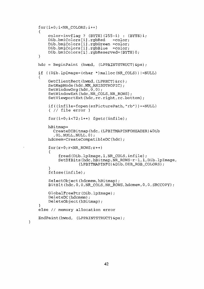
The following code fragment shows a way to display a greyscale image, by defining aDIB information header and a greyscale palette. The image scanlines are inserted in thepicture line-by-line, because the compiler had no support for large bitmaps (> 64k) at thetime of release. The freeing of pointers and deleting of windows objects is important toprevent the memory from flooding with unused data objects.
In this chapter the functionality of the low-level vision algorithms will be evaluated. Theperformance of the complete VSS system will be compared to the requirements defined inChapter 1. Proposals to overcome the flaws of the VSS at the cost of operator interventionwill be made. Finally some recommendations will be made and methods not yetinvestigated will be proposed.
7.1 Edge detection
The performance of edge detection depends on setting the threshold parameter to find abalance between too many noise pixels and poorly visible object edges. Lee's method [15]of separating horizontal and vertical scan-direction and perform one-dimensional edgedetection produces accurate results. The method of adjusting the threshold to the numberof edgepoints found suffices, although this introduces a new parameter, the desirednumber of edges. This new parameter is less sensitive. Good illumination of the workpieceproved to be the key-factor to obtain a complete line-image of the workpiece. Requirementis that all object edges are visible. While this requirement cannot be met in practicalsituations, a photometric stereo method was successfully designed to produce multipleimages in which each edge is visible in at least one image (Chapter 3, section 3.6). Themost interesting result of this method is that edges that are visible in multiple images areextracted very accurate, and that noise is suppressed because it has no cross-imagecorrelation.
Not yet investigated is if the accuracy is equal for every line direction. It is expected thatthe highest accuracy is reached if the line direction is perpendicular to the scan-direction.An extension to the current method of edge detection could be a two-dimensional edgedetection based on the results of line extraction. In this scheme, for every extracted line, acustom 2-dimensional kernel could be calculated that is able to detect edges in the direction of the extracted line. With these kernels, all edges could be re-detected with thespecial kernel that is optimized for that particular line direction. After this, the lines shouldalso be re-extracted, to produce more accurate results. It is expected that such a methodwould be less be insensitive to noise.
7.2 Line extraction
The line extraction algorithm is fast and accurate. Depending ononly three parameters, the algorithm produces complete line images if the edge image is complete, i.e., all object edges have beendetected and there are few noise pixels. In practice this is notalways the case. Because the algorithm searches in the environment of a predicted pixel location if an edgepixel was not found, itwill not abort on small disturbances in the edge image. A draw- Figure 7.1: Corner ofback of the line extractor is that the endpoints of the line do not a cube (edgepixels)coincide with the actual corner edge. The lines are usually tooshort. This is caused by poor perfonnance of the edge detector, when the distance between
43
two edges is less than the filter size. Figure 7.1 shows part of an edge image of the cornerof a cube. Near the actual cornerpoint the edges seem to diverge from that point. The lineextractor will terminate the extracted line once subsequent pixels cannot be found in theregion determined by the parameters. It should be noted that this is a problem to be solvedduring edge detection or post-processing rather than during line extraction.
7.3 Post-processing
The post-processing tool is very useful to reduce the number of lines. By setting itsparameters very strict, it becomes a transparent filter. The parameters should not allow toomany lines to be merged, to prevent lines that belong to different object edges to bemerged into one line. The post-processing could be extended to perform additional optimizing, like the manual operations described in Chapter 5 section 3. For example, endpoints of different lines could be merged if they fall inside a circle-shaped window thatslides across the screen. This would perfectly connect the corner of the cube in figure 7.1.
7.4 Implementation of a User Interface
The Windows user-interface as it has been implemented proved to be a successful development decision. The VSS now fully utilizes Windows graphics to display its graphicaloutput. Furthermore, every member of the project team can operate the VSS, becauseevery module has the same operating scenario. Another development goal that has beenachieved is that the algorithms themselves are separated from the tTl. Future enhancementsthat are made to the tTl must guarantee that this crucial piece of software remainsmaintainable.
7.5 Suggestions for future research
2D Edge detection - Improvements to the current algorithms can be made in severalways. The functionality of the algorithms can be improved by making little modifications,or whole new paradigms could be added. A two-dimensional edge detector, as proposed insection 7.1 can be seen as a modification of the current edge detector.
Subpixel accuracy - As mentioned in section 4.4.2, an accuracy analysis should indicatewhether it is useful to employ subpixel accuracy. It is expected that the least-squares fit ofa line to a (large) set of pixels will cancel out the rounding errors, introduced by the useof integer pixel coordinates rather than subpixel-accurate coordinates.
Region-growing - A whole new approach for low-level vision would be employing aregion-growing algorithm. Schutte [14] found that object texture causes this algorithm tofail, but it is expected that the average object in the workpiece will have a plain surface.Region-growing might therefore be very suitable. A constraint for the region borders couldbe to require them to have the shape of a polygon with a fixed maximum of edges.
Ellipses - An extension to the current line-extraction algorithm would be the ability todetect curved line segments and model them as parts of ellipses. Broertjes [3] had someproposals for this, and there is some literature [22,27]. The straight lines should bepreferred to the curved lines. A way to accomplish this would be to fit curved lines only
44
to the edgepixels that were not used in the straight line extraction. This would also implythe advantage of not having to modify the original line extraction algorithm at all.Currently the shape of the workpieces for the robot welding system does not call forimmediate support of curved line segments.
Lighting - A drawback of using multiple light sources is the presence of a large numberof shadow-lines on the object, which will result in unwanted lines. Although it is veryeasy to remove the influence of ambient light by subtracting it from the 'illuminated'image, this lighting sometimes yields the best VSS results. A method of separating thelines caused by shadows from the 'real' object edges could be to position two lightsources close to each other, yielding two line images. The 'shadow' lines will havedifferent positions, and the 'real' lines will be approximately the same.
Processing time - In Chapter 2, section 2.8 it was recognized that the larger part of thetime a survey takes is spent performing user interaction. This interaction should beeliminated before any improvement in the automatic part of the VSS is beneficial. Anotherapproach would be to allow the VSS to be semi-automated. In practical situations, humaninteraction proved to be necessary to produce reliable results. The capabilities of the VSScould be improved if the operator handles decisions between selecting and discarding.Note that calibration operations are always similar and could easily be automated.
45
References and relevant literature
[1] Farro, M.J.Straight line detection in low contrast images: Theory and application. M.Sc.Thesis, Eindhoven University of Technology, Measurement and Control Section(1992)
[2] Buts, P.J.H.Edge detection from noisy images for 3D scene reconstruction. M.Sc. Thesis,Eindhoven University of Technology, Measurement and Control Section (1993)
[3] Broertjes, R.A.J.Extracting straight lines and elliptic arcs from edge images. M. Sc. Thesis,Eindhoven University of Technology, Measurement and Control Section (1993)
[4] Kaptein, E.M.J.Knowledge-based Scene Analysis from Line Images. M.Sc. Thesis,Eindhoven University of Technology, Measurement and Control Section (1993)
[5] Kaptein, E.M.J.Structural Matching in knowledge-based 3D scene reconstruction. Journal A: vol.34, no 4, pp. 17-24. (1993)
[6] Tjoa, E.K.L.Geometrical Matching of 3D deformable models. M.Sc. Thesis,Eindhoven University of Technology, Measurement and Control Section (1993)
[7] Smook,O.E.F.Camera Position Calibration Using the Image of Known Object EdgesM. Sc. Thesis, Eindhoven University of Technology, Measurement and ControlSection (1994)
[8] Korsten, H.P.J.Improving Synthetic Image Modeling by optimizing the reflection model.M. Sc. Thesis, Eindhoven University of Technology, Measurement and ControlSection (1994)
[9] Petzold, C.Programming Windows 3.1. 3rd ed. Microsoft Press (1992)
[14] Schutte, K.Knowledge Based Recognition of Man-Made Objects. PhD. Dissertation UTEnschede. (1994)
[15] Lee, D.Edge detection, classification, and measurement. IEEE Computer Society Conferenceon Computer Vision and Pattern Recognition, 1989, San Diego, California, USA,
4-8 June 1989. P. 2-10.
[16] Weng, J., Cohen, P. and Herniou, M.Camera Calibration with distortion models and accuracy evaluation. IEEE Trans.on Pattern Analysis and Machine Intelligence 14: pp. 965-980, 1992
[17] Burns, J.B., A.R. Hanson and E.M. RisemanExtracting straight lines. IEEE Trans. on Pattern Analysis and Machine Intelligence, vol.8, pp. 425-455 (1986)
[18] Duda, R.O. and P.E. HartPattern Classification and Scene Analysis. New York: John Wiley (1973)
[19] Giraudon, G.An efficient edge following algorithm. Proc. 5th. Scandinavian Conference onImage Analysis, vol.2, pp. 547-554, Stockholm, Sweden (1987)
[20] Han, M.H., D. Jang and J. FosterIdentification of cornerpoints of two-dimensional images using a line search method. Pattern Recognition, vol.22, no. 1, pp. 13-20 (1989)
[21] Haralick, Robert M. and Linda G. ShapiroGlossary of Computer Vision Terms. Pattern Recognition, vol.24, no.2, pp. 69-93(1990)
[22] Liang, PingA New Transform for Curve Detection. Proc. third International Conference onComputer Vision, pp.748-751 (1990)
48
[23] Lie, W. and Y. ChenRobust line-drawing extraction for polyhedra using weighted polarized Houghtransform. Pattern Recognition, vol.23, no.3/4, pp. 261-274 (1990)
[24] Marr, D.C. and E. HildrethTheory of Edge Detection. Proc. Roy. Soc. London, vol. B 207, pp. 187-217 (1980)
[25] Proceedings of SPIE- The international Society for Optical Engineering: Optics,Illumination and Image Sensing for Machine Vision, vol.728, pp. 35-129 (1987)
[26] Roberts, L.G.Machine perception of three-dimensional solids, Optical and Electro-optical Information Processing, pp. 159-197. Tippet, J.T. et al. (eds.). MIT Press, Cambridge,MA (1965)
[27] Rosin, Paul L. and Geoff A.W. WestSegmenting Curves into Elliptic Arcs and Straight Lines. Proc. third InternationalConference on Computer Vision, pp.75-82 (1990)
[28] Shirai, Y.Edge finding, Segmentation of edge and recognition of complex objects. Proc. 4th.International Joint Conference on Artificial Intelligence, vol.2, pp. 674-681, Tbilisi,Georgia, USSR (1975)
[29] Shirai, Y.Three-dimensional computer vision. Berlin, Heidelberg, New York: Springer-Verlag(1987)
[30] Turner, K.J.Computer Perception of Curved Objects Using a Television Camera. Ph.D. Thesis,School of Artificial Intelligence, Edinburgh University (1974)
[31] Williams, C.M.Bounded straight-line approximation of digitized planar curves and lines. ComputerGraphics and Image Processing, vo1.16, pp. 370-381 (1981)
[32] Zucker, S.W., A. Rosenfeld and R.A. HummelAn Application of Relaxation Labeling to Line and Curve Enhancement. IEEETrans. on Computers, vol.C-26, p.394 (1977)
[33] Zhang, R. et aI.,Analysis of Shape from Shading Techniques. IEEE CVPR-94, Seattle, Washington,June 20-24 (1994)
[34] Tagare, H.D. and deFigueiredo, R.J.P.Non-Lambertian shading and photometric stereo. Proceedings of the SPIE - TheInternational Society for Optical Engineering, Vol: 1260 (1990), pp.100-111.
49
[35] Kozera, R.Existence and uniqueness in photometric stereo. Applied Mathematics and Computation, Vol: 44 (1991), Iss: 1, pp. 1-103
[36] Sakane, S. and T. SatoAutomatic planning of light source and camera placement for an active photometricstereo system. Conf. Proceedings. IEEE International Conference on Robotics andAutomation, IEEE Comput. Soc. Press USA (1991) pp. 1080-1087.
50
Appendix AFrame grabber access
The frame grabber equipment can be considered a specialized piece of hardware. To beable to utilize other frame grabbers in the future, the access to the frame grabber shouldbe kept separate from the rest of the software system that depends on it. To this end anumber of basic frame grabber operations have been defined. Although different frame grabbers will support many more advanced actions, the basic operations will be supportedby most of them. The software system accesses the frame grabber by issuing one of thebasic operations to a specialized access program, which has to be rewritten for every typeof frame grabber used. The basic operations are:
O. Initialization. Upon receipt of this command, the frame grabber can perform all itsinitializing actions.
1. Live image. This command connects the video source to the frame grabber monitorfor image previewing.
2. Freeze. This command digitizes the image into the frame grabbers' memory.
3. Select camera. If the hardware supports multiple video sources that can be selectedby software, this command is used to select a video source.
4. Load image. If images can be loaded from a storage device into the framegrabbers' memory, this command accomplishes it.
5. Save image. The digitized image stored in the frame grabbers' memory is saved toa storage device.
The access program implemented for the Philips SBIP-2 image processor [13] is calledsbip. exe and takes two command-line parameters:
Syntax: sbip 0 <x> Initialize SBIP-2 «x> don't care)sbip 1 <n> Live picture from camera <n>sbip 2 <x> Freeze image «x> don't care)sbip 3 <n> Select camera <n>sbip 4 <filename> Load image from file into SBIP-2 memorysbip 5 <filename> Save image from SBIP-2 memory to file
51
Appendix BAdministration of VSS files
B.t Introduction
Because of the modular structure of the VSS. a large number of files will exist simultaneously while operating the VSS. If different workpieces are surveyed with differentcameras at multiple locations. the need emerges to be able to link each unique situationwith one unique filename. Because the diversity of files is multidimensional (i.e.• imagesmay be categorized in camera number. workpiece session. camera location. lightingconfiguration etc.) the administration scheme will be non-trivial and complex. The task ofthe user-interface is to allow the user to select the categories of the input image. The'supervising' part of the user interface will compose a unique filename. and handles alladministrative actions. for instance. how many images have been taken up to now. whichcalibration information belongs to which image. which translation matrix belongs to whichcamera position and so forth. The administration scheme is presented below.
B.2 Definitions
The degrees of freedom that determine a file within the VSS are:
By choosing one element from the sets associated with each entity. a unique VSS-filenamecan be composed. We define the term session as the collection of data referring to onestatic configuration of objects (workpiece) in space. This data may have been obtained bymultiple configurations of elements from the sets mentioned above.
One simplification is to join the camera number and camera location sets. and to form oneunique imagenumber from it. This is allowable if the administration links the correctcalibration info to each image. The explicit original camera number is lost. but implicitlydefined by the calibration information.
The lighting configuration requires a separate list which can be indexed to obtain aconfiguration instance. E.g.• index 'a' could refer to 'on-off-off-off; index 'b' to 'off-onoff-off' etc. in case of four switched light sources.
The file contents are determined by the extension. Current extensions are:
.ses:
.img:
.lmc:
.hpo:
Session informationGrey level image. uncorrectedGrey level image. after lens correctionHorizontal edges position
53
.vpo:
.lex:
.ldr:
.edf:
.tm:
.sma:
.gma:
Vertical edges positionExtracted lines before post-processingExtracted lines after post-processingCamera description file (calibration data)Camera position file (translation matrix)Structural matching outputGeometrical matching output
Associated with a session is one unique, user selected, session that can be used as a prefixfor all file names of (intermediate) results of the VSS. We associate with a session a count'number-oj-images' that indicates the number of images retrieved from a given scene anda count 'number-oj-cameras' that specifies how many of the available physical camerasare used. We now define a VSSlilename according to the DOS file name format:
With1 :::; imagenumber :::; number-oj-images,2 :::; Length(scenename EB imagenumber) :::; 8'a' :::; lighting-conjig :::; number-oj-lighting-configsand an extension identifying the contents of the file.The lighting configuration suffix is optional because the different lighting configurationswill produce one edge image, e.g., 'testla. ime' thru 'testle. ime' will produce'testl.hpo'.
A scene is will consist of a number of files with VSSlilenames, with one file namedsessionname. ses that can be inspected at all times to find out which VSS-filenames mustexist.
The structure of sessionname . ses is straightforward:
NOTE: The lighting configuration information is not currently implemented in the VSS.
Examples of filenames:
eube7b. ime:
testl.sma:
Corrected grey level image #7 of a session named 'cube', usinglighting configuration 'b'.
Structural matching output of image #1 of a session named 'test'.
54
Appendix CDescription of file formats
C.I Review of files used in the LLV part of the VSS
The VSS uses a collection of datafiles that provide the transportation of informationbetween subsequent VSS-(sub)modules. The format of these datafiles defines the interfacebetween these modules and should provide an unambiguous description of the output dataof the file's deliverant. Also this interface should be as thin as possible, i.e., no redundantinformation should be present in the file. In this appendix the file formats related to thelow-level submodules are described. These are:
• Image files (SBIP2-format, size 256K)• Parameter files (ASCII-format, size less than 1K)• Camera description file (ASCII-format, size less than 1K)• Lines file (ASCII-format, size less than 10K)
C.2 Image file format
The image files generated by the SBIP2 software [13] are compatible with the ITEXPCpIus of Imaging Technology. The 512x512 bytes rasterdata are preceded by thefollowing "Image file header":
byte#
0,12,34,56,78,910,1112,1314..6364..nn+l..m
Contents:
ID-field containing "1M"Comment field length (max. len. 200 including \0 char), lsb firstImage width, lsb firstImage height, lsb firstX-coordinate of the upper left corner of the imageY -coordinate of the upper left corner of the imageFile type flag, O=normal, l=compressed (NOT supported for SBIP2)Reserved (leave 0).Comment field. Length is specified by bytes 2,3. Contains the image name.Image data, one byte per pixel.
If a standard comment field of eight bytes is maintained, the image data can be reached byskipping the first 72 bytes. Although this is not an elegant way, it enables commercialgraphics packages like 'PictureMan for Windows' to read the file as a 512x512 byte arraywith byte offset 72, and convert it to any other popular file format (GIF, TIFF, PCX, BMPetc.).
C.3 Parameter files
A standard parameter file format has been proposed and implemented to provide a channelto transport parameter values from the user interface to the application (a VSS(sub)module). In this file, parameters are identified with their name, value and type. The
55
application only reads the value. The user interface provides a graphical way of editing theparameters by reading all three fields. A type field is included to allow special parametersto be translated into graphical intuitive windows elements (e.g., a boolean type parameteris translated into a windows checkbox; a file type parameter is translated into a windowscombo-box).
The layout of a parameter file with n parameters is as follows:
n ParameterSetNameo Po1 PI2 pz
n-lo12
n-l
Pn-I"Pnameo""Pname l "
"Pnamez"
"Pnamen_I "
PtypeoPtype l
Ptypez
Ptypen_1
The name of the set of parameters is 'ParameterSetName', and serves only for documentation purposes. Ptype j , can be any of: "i" (int); "b" (bool); "f' (float); "F" (File) or "s"(string).
The following hypothetical parameter set illustrates the layout of the file:
Both the intrinsic and the extrinsic calibration parameters are stored into a . CDF file. Thestructure of this file is such that additional calibration information can be added in a laterstage. Details on this can be found in [7]. A typical camera calibration file is listed below:
The camera parameters (S,C,f,D,T) are assigned a status, which indicates how the valueshave been attained:
N=not availableE=estimatedA=calibratedS=stated
c.s Lines file
The sets of line segments produced both by the line extraction algorithm (LINEX, . 1ex)and the postprocessing algorithm (CONNECT, .ldr) obey the D3D line format. Thisgeneral format allows for 2-D and 3-D line and plane description. Only a format for the 2D line description is used here. The file first lists a number (n) of vertices, and thendefines the indices of the vertices that compose a line:
1.2.
n. Xn YnFaces:sJ eJ.
S2 e2•
If every line has individual begin- and endpoints, there are m=nl2 lines. (Xi ,Y) are thebegin- or endpoints that can be specified as floats, in case of subpixel accuracy. In thefollowing example, four line segments that form a box are specified using the . LDR fileformat:
1. 50 1002. 100100
57
Appendix DPostScript utilities
Two utilities have been developed to provide high-quality output of the Low Level Visionrelated output files: the greyscale images and the line segments images. The description ofthese images in the PostScript language was derived from [10] and [11]. The PostScriptlanguage is a stack-oriented language, like for instance Forth, that provides all facilities amodern typesetter needs to produce professional documents. PostScript files are not veryefficient in terms of compactness, but the language provides a powerful device-independent document description.
D.I Grey-level to PostScript conversion
The file starts with the standard PostScript header.
%!PS-Adobe-2. 0
After this, a font is selected, scaled and set, to enable text output on the page.
/Times-Roman findfont10 scalefontset font
At the typesetter a storage buffer is defined to 'heave' the image data from the file intothe typesetter raster. The (arbitrary) size is chosen to fit one scan line at a time.
/grstr 512 string def
The device context is saved on the stack with the gsave command, and later restoredusing the gres tore command. This leaves the typesetter in an identical state afteroperation.
gsave
The typesetter's coordinate system ongm is translated to the lower left corner of thegreyscale picture. The unit of the coordinate space is scaled to the desired dimension. Thisdimension is specified in units of 1/72 inch=0.35 mm. The values used below are arbitraryvalues, yielding a 3% inch wide picture with an aspect ratio of 0.75.
20 458 translate252 189 scale
The following commands define the actual 512x512x8 greyscale image. The commandsinstruct the parser to look for the hexadecimal image data at the end of the current file.
The name of the image is printed just below the lower left corner of the image.
o -11 moveto(name of the image) show
After this, the graphics state of the typesetter is restored, and the 8192 lines ofhexadecimal encoded image data (2 hex. digits per byte) are followed by the showpagecommand.
grestore
% Start of image data3a3234343632333334353331333 .... 8192 lines of hex data ... . 438373a3a3837393c3d38373936
showpage%EOF
In this way, multiple images can be displayed on one page. The size of the PostScript filewill be several megabytes. Note that most PostScript printers are occupied more than 15minutes for every image because of the vast amount of data they must handle.
The PostScript translation described above has been implemented in a utility calledimg2ps. This utility renders a maximum of 6 images on one page (which can be adjustedeasily in the source code by changing a #define directive). Syntax can be obtained byrunning the utility without command-line parameters.
D.2 Line image to PostScript conversion
Line images can be output in higher quality using PostScript compared to conventionalmethods like making a screen-dump or snapshot of the screen. The ldr2ps utilitytranslates the line segments in the input file directly into line drawing commands at thetypesetter's resolution, thus guaranteeing the least amount of aliasing along the lines. Thestructure of the PostScript file resembles the previously described PostScript bitmap imagefile.
First of all, the standard PostScript header is output and the current drawing path iscleared.
%!PS-Adobe-2.0newpath
The origin is translated to the desired location on the paper, and the size of the picture isdetermined by scaling the axis. In this example, the image is scaled to 10.0x7.5 cm, whichis the correct aspect ratio for SBIP2 images. Note that the translation is with respect of thelower left corner of the page, and that there is a margin around the page that cannot beprinted on.
60
18 18 translate283.5 212.6 scale
Coordinates in the domain [O,I]x[O,I] will be mapped onto the 1O.0x7.5 em area. Thisimplies that now lines of any resolution can be displayed by dividing their coordinates bythe horizontal and vertical resolution, respectively (512 and 512 in this case). Themaximum typesetter's resolution can be utilized by selecting a zero line-width.
o setlinewidth
To save some disk space, the sequence of moving the 'pen' to the startpoint and drawing aline to the endpoint is abbreviated by defining a PostScript macro (' 1 ')~
/1 { moveto lineto stroke } def
A frame around the picture can easily be accomplished by the following sequence.
o 0 0 1 1o 1 1 1 11 1 1 0 110001
After this, the image lines are specified as accurate as possible.
The page will be printed after the showpage command is read.
showpage%EOF
A more advanced piece of PostScript code can be employed to calculate the maximumscaling that the printing device can handle. This cannot be preset if the file is to be deviceindependent. For details, refer to the PostScript reference manual [10]. The code willmerely be listed here. The page margin is assumed to be 18 PostScript points (18/72 Inch)wide.
clippath pathbbox pop exch pop exch sub 36 sub dupdup clippath pathbbox 4 1 roll pop pop popexch sub 18 sub18 exch translatescale clearnewpath