Eindhoven University of Technology MASTER Nonlinear model predictive control of a copolymerization process using hybrid modeling Stapel, P.J.A. Award date: 1998 Link to publication Disclaimer This document contains a student thesis (bachelor's or master's), as authored by a student at Eindhoven University of Technology. Student theses are made available in the TU/e repository upon obtaining the required degree. The grade received is not published on the document as presented in the repository. The required complexity or quality of research of student theses may vary by program, and the required minimum study period may vary in duration. General rights Copyright and moral rights for the publications made accessible in the public portal are retained by the authors and/or other copyright owners and it is a condition of accessing publications that users recognise and abide by the legal requirements associated with these rights. • Users may download and print one copy of any publication from the public portal for the purpose of private study or research. • You may not further distribute the material or use it for any profit-making activity or commercial gain
Transcript
Eindhoven University of Technology
MASTER
Nonlinear model predictive control of a copolymerization process using hybrid modeling
Stapel, P.J.A.
Award date:1998
Link to publication
DisclaimerThis document contains a student thesis (bachelor's or master's), as authored by a student at Eindhoven University of Technology. Studenttheses are made available in the TU/e repository upon obtaining the required degree. The grade received is not published on the documentas presented in the repository. The required complexity or quality of research of student theses may vary by program, and the requiredminimum study period may vary in duration.
General rightsCopyright and moral rights for the publications made accessible in the public portal are retained by the authors and/or other copyright ownersand it is a condition of accessing publications that users recognise and abide by the legal requirements associated with these rights.
• Users may download and print one copy of any publication from the public portal for the purpose of private study or research. • You may not further distribute the material or use it for any profit-making activity or commercial gain
Nonlinear Model Predictive Control of a Copolymerization Process
using Hybrid Modeling
P.J.A. Stapel
NR-1994
Februari 6, 1998
Dr.ir. R.J.P. van der Linden Ir. G.Z. Angelis
Abstract
Polymer is a very important product and is produced on a large scale. The diversity of polymers is very big and ranges from nylons, vinyls and rubbers to polyesters and acrylics. The diversity is caused by the fact that a polymer build from a certain type of (co )monomers can have different properties, for example different viscosities. This gives rise to the main problem of producing polymer: to obtain a product of certain processing and end-use properties. The two most important polymer properties are the melt index, which is a measure for the viscosity, and the density.
A polymerization plant often produces a wide range of different grades to suit marked demand. This causes the problem of the grade changes, i.e. switching from one product to another. Grade changes are slow, and the polymer produced during the grade changes is off-spec and must he sold for a lower price than the regular product within specification.
In this thesis research was clone to the application of Nonlinear Model Predictive Control (nlMPC) to control the polymer properties. nlMPC is a model based controller and needs an accurate model of the process. A nonlinear model of the process was developed using hybrid modeling techniques, i.e. combining both first-principles models and neural networks. After validation the hybrid model was used in the nlMPC.
Simulations showed that, provided that an accurate model of the process is available, nlMPC can he used for cantrolling the polymer properties both to speed up grade changes and to compensate for unmeasured disturbances.
Acknowledgments
This report is the result of a one year research for rny rnaster thesis at the Systerns and Control Group of the faculty Applied Physics of the Eindhoven University of Technology (TUE). I would like to thank everybody of the Systerns and Control Group for rnaking rny stay a pleasant one.
I especially want to thank rny direct coach at the TUE, Georgo Angelis, for helping me with rny daily problerns, neural network questions and for his fitness training advises, rny coach at DOW, Jan Willern Verwijs, for his enthusiasrn and for answering all rny questions about chernistry and the polyrnerization process and rny coach at TNO-TPD, Wim Bournan, for his MPC ad vice and his fast responses. I also want to thank Ruud v.d. Linden for letting me workat this project, and for his input, tagether with Rene v.d. Molengraft, at the twoweekly meetings.
Frorn TNO-TPD I would like to thank Walter Renes for his help in the early stages of rny research when I had problerns with the DEC Alpha workstation.
Special thanks go toErwin Siefken of Advansys, whogave me the freedorn and trust, to manage rny own working hours, which made it possible for me to combine bath doing rny rnaster thesis research with a part-time job as an ernbedded software engineer at Advansys.
Arnong all the students in the Systerns and Control Group there is one which I would like to thank with ernphases, Casper Wassink. Because of the sirnilarities in our research subjects there was a lot of cooperation.
Finally I greet every student who did his graduation research at the Systerns and Control Group during the time I was also working there, Gerwald, Frank, Gert, Joost, Mathieu, Udo, Agnes, Meike, Ignace, Rernco, Reinout, Wouter, Alex, Pirn.
I
l
Contents
1 Introduetion 1 1.1 Goal of this Research . 1 1.2 Frameworkof this Research 1 1.3 Outline of this Thesis . 2 1.4 Technology Assessment . . 3
6 The Copolymerization Process 37 6.1 Introduetion . . . . . . . . . . . 37 6.2 Introduetion to Polymers . . . 37
6.2.1 Polymers and Polyethylene 37 6.2.2 Polymer Properties: Density, MWD and Melt Index 38
6.3 The Polymerization Process 40 6.3.1 Reaction Kinetics. . 40 6.3.2 Reactor Description 41
6.4 Control Problem . . . . . . 42 6.4.1 Control Objectives . 42 6.4.2 Current Control of the Process 43 6.4.3 MPC of Polymerization Processes Described in Literature 44
6.5 Implementation of the Process in gPROMS . . . . . . . . . 45
7 Modeling and Control of the Copolymerization Process 47 7.1 Application of nlMPC to the Polymerization Process 47 7.2 First Identification Experiments . . . . . . . . . . . . 47
8.2 Recornrnendations . . . . . 8.2.1 General ...... . 8.2.2 Polyrnerization Case
A Reactor Description
B ldentification Experiments
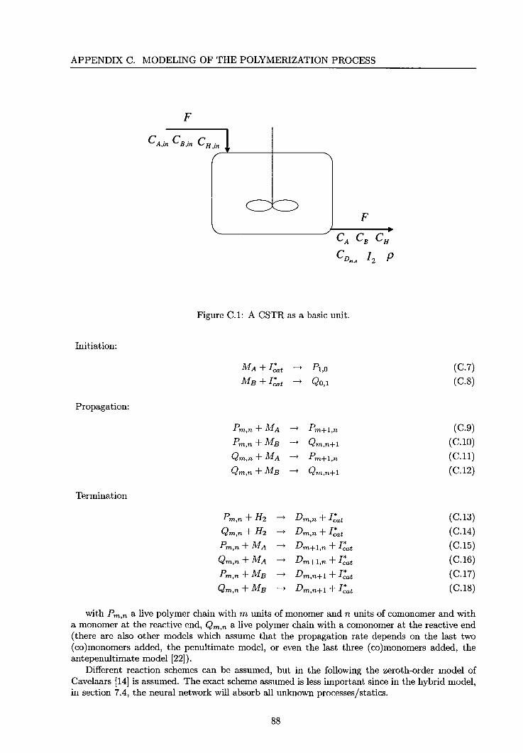
C Modeling of the Polymerization Process C.1 Derivation of the Model . . . . . .
C.l.1 General Description ....... . C.l.2 Long Chain Approxirnation ... . C.l.3 Mornents of the Molecular Weight Distribution C.l.4 Copolyrner Properties . . . . . . . . . .
C.2 Model Used ................... . C.3 Literature on Polyrnerization Process Modeling
D Linearizing the Hybrid Neural Net for MPC D.1 The MPC Algorithrn ............. . D.2 Linearizing the Wiener Neural Network Model
E Modeling Using Neural Networks and a Priori Knowledge E.1 Introduetion .......................... . E.2 Incorporating a Priori Knowledge into the Neural Network.
Model predictive control (MPC) is an advanced control algorithm which is widely applied in petrochemical industry. MPC is a model based controller which uses a model of the process to pred.iet the future behavior of the process during a certain time interval and calculates the optimal control moves which are needed to achleve the desired control objective. An advantage of MPC is that it can handle multivariable systems and can handle constraints on the process and the manipulated variables.
Application of MPC in practice is still limited to linear models. In this project a nonlinear controller, using a nonlinear model of the process, will he investigated. To give the research a practical component a case was studied which involves a polymerization process. The polymerization process is a highly nonlinear process of which the properties of the polymer should he controlled.
For the MPC controller to he used a nonlinear model of the process needs to he developed. For this purpose a hybrid modeling approach will he used, i.e. a combination of a white-box (physical) model with a neural network.
The aim of this research can he formulated as: to examine the possibility of nonlinear model predictive control for the application of polymer property control in a polymerization process, using hybrid neural models.
1.2 Frameworkof this Research
This research is a combination of the research interests of three different parties. First of all is the Ph.D. research of ir. G.Z. Angelis at the TUE. Subject of his research project is the identification of nonlinear systems for control application with the use of combined first-principles modeling and black-box (neural) modeling techniques, in which the a priori knowledge of the system is used as much as possible. The aim of his research is to improve the pred.ietion capabilities of the model by means of hybrid system modeling. The project focuses on the identification of models that can he used in Model Predictive Controllers (MPC's), as MPC's require accurate pred.ietion of the system behavior over a long future horizon, the hybrid models to he derived should accurately describe the dynamics of the system by simulation.
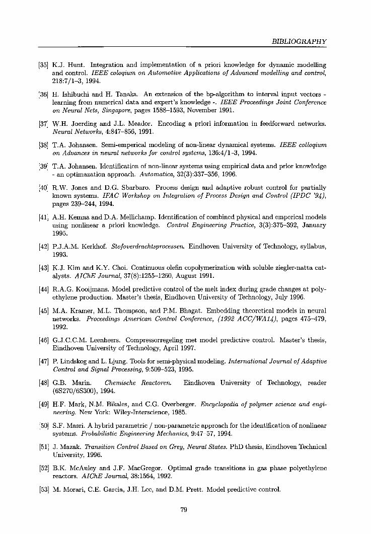
The Ph.D. research of Angelis is in cooperation with TNO-TPD, which has developed an MPC algorithm. The MPC algorithm is integrated in a software package called PRJMACS. PRJMACS is a real time software package developed at TNO-TPD which is used in industrial processes to measure and collect data, which afterwards can he used for model purposes and controller design. The last few years lots of research has been done invalving the application of MPC. MPC has been successfully tested on several cases: fluidized catalytic cracker ([59]), thermohydrolic example process ([81], [78]) , compressor station ([67], [46]), glass furnace ([83]).
1
CHAPTER 1. INTRODUCTION
smaller gPROMS process
model
I I PRIMA CS PRIMA CS
---• MPC module
I I MPC module
gPROMS model
(a) (b)
Figure 1.1: Experimental setup_ (a) Simulation environment used in this research; (b) Real plant set up_
The last party involved is DOW Benelux_ The interests of DOW Benelux go to direct polymer property controL Polymer is a very important product and is producedon a large scale. The diversity of polymers is very big and ranges from nylons, vinyls and rubbers to polyesters and acrylics. The diversity is caused by the fact that a polymer build from a certain type of (co )monomers can have different properties, for example different viscosities. This gives rise to the main problem of producing polymer: to obtain a product of certain processing and end-use properties. The two most important polymer properties are the melt index, which is a measure for the viscosity, and the density. Often a wide range of different grades is produced at one polymerization plant to suit marked demand. This causes the problem of the grade changes, i.e. switching from one product (polymer with certain properties) to another (polymer with different properties). Grade changes are slow, and the polymer produced during the grade changes is off-spec and must he sold for a lower price than the regular product within specification.
A feasibility study on the application of model predictive control of a polymerization process was done by Umans [78]. He tested MPC on a thermohydrolic example process which has the same control problems as the polymerization process, i.e. control of unmeasured outputs, dynamic optimization of a change in setpoint, reduce of interaction, take in account process constraints. He concludes that MPC should he suited for cantrolling the polymerization process when an accurate model of the process is available.
In this case study the controller was not tested on the real plant. Instead a rigarous fi.rstprinciples simulation model was used which is derived from a larger simulation model that describes the real plant. The first-principles model was developed in gPROMS, a software package especially designed for rnadeling dynamic systems, and runs on a workstation. The larger gPROMS model can be connected to the real process via PRIMACS for validation purposes. The final aim is to control the real process using the MPC module from PRIMACS (figure 1.1).
1. 3 Outline of this Thesis
This research has several key elements, i.e. neural networks, hybrid modeling, nonlinear model predictive control, which should be explored thoroughly before the step can be made to the case study, the polymerization process. The topic of neural networks is first discussed in chapter
2
...
1.4. TECHNOLOGY ASSESSMENT
2. The potential of neural networks to approximate nonlinear functions and the application of neural networks rnadeling nonlinear dynamic systems is discussed. In chapter 3 hybrid rnadeling is treated. The chapter is the result of an extensive literature study on the topic of combining white-box rnadeling techniques with neural networks, i.e. hybrid modeling. Different approaches and model structures which were found in literature are presented. The next chapter, chapter 4, gives an introduetion to Model Predictive Control (MPC). Several aspects of MPC are discussed, including the basic idea behind MPC, tuning aspects and nonlinear MPC to control nonlinear processes.
Chapter 5 is about identification. When met with an unknown process which should he modeled (in this case the polymerization process) there are certain well defined steps which can he executed togainas much insight a bout the static and dynamic behavior of the process as possible. Important issues are experiment design and the choice of a black-box model structure. A special hybrid model structure is discussed, with linear dynamics in series with a static neural network ( often referred to as a Wiener model structure), and a 2 stage parameter estimation procedure for the hybrid model structure is presented.
Finally the case study, the copolymerization process, is presented in chapter 6. Polymers and polymer properties are shortly discussed and the polymerization process itself is outlined. The control problem is pointed out and some attention is paid at the current control of the process.
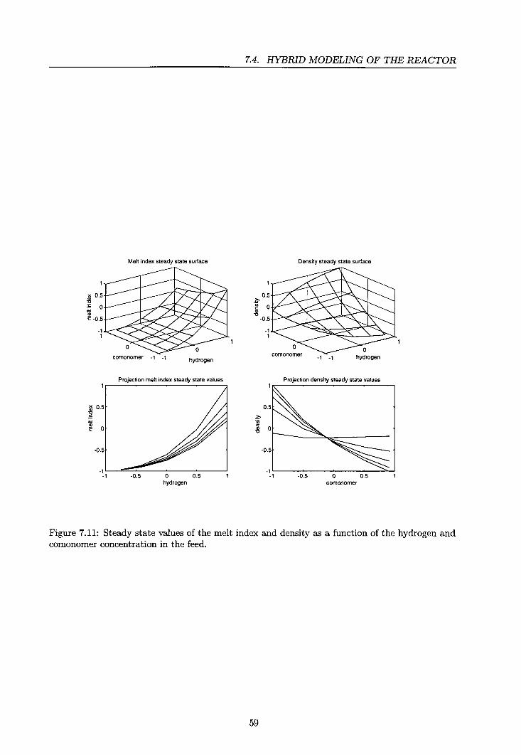
The actual results are presented and discussed in chapter 7. The inputs are selected which can he used for cantrolling the polymer properties and a hybrid model is derived. After validation of the hybrid model, the model is implemented in the MPC. Finally the MPC is tested on the process by performing grade changes and other control tasks. The chapter ends with a discussion.
The last chapter, chapter 8, contains the conclusions and recommendations for further research.
1.4 Technology Assessment
The main problem with polymer plants are the grade changes, i.e. switching from producing one product to producing another product.
Sinclair [70] has noted three basic aspects of a grade change that determine cost penalties. First, there is often a reduction in plant output during a grade change transition to maintain safe operating conditions. For example, in a high-pressure free radical polymerization of ethylene to low density polyethylene, a grade change at normal production capacity can result in reactor temperature or pressure runaway. The second cost issue relates to the off-spec product produced during the grade transition that must he sold for lower price than the regular product within specification. Finally, economie costs are incurred due to the rnainterrance of product inventories, which are necessary to ensure sufficient supplies of each grade while the reactor is producing other grades of the product slate.
Obviously the reduction of off-spec product can result in a significant reduction in the total production cost of the product illustrating the need for efficient transitions between reactor grades. This is particularly true for processes with large reactor resident times and short production runs.
McAuley and MAcGregor [52] have stuclied the optimization of grade transitions for linear lowdensity polyethylene in a commercial fl.uidized-bed reactor. They conclude that any optimization strategy must consider the economie conditions of the market. During periods of high market demand, it may he preferabie to reduce the grade transition time as much as possible. In periods of low market demand, however, a policy which produces less off-spec material at the expense of a longer transition time may he preferred .
3
CHAPTER 1. INTRODUCTION
4
Chapter 2
Introduetion to Neural Networks
2.1 Introduetion
In this chapter neural networks are introduced which are used in modeling and system identification. In the first section an introduetion will be given from the biologica! analogy. After this artificial neural networks for function approximation are discussed. Also attention is paid to the training of neural networks. In section 2.5 different ways of modeling dynamic systems will be discussed, using dynamic neural networks. The chapter ends with a review and some considerations. Termsof neural network jargon are introduced and discussed.
2.2 From Biologica! Neural Networks to Artificial Neural Networks
2.2.1 Biologica! Analog
Workon artificial neural networks, commonly referred to as 'neural networks', has been motivated right from the beginning by the recognition that the brain computes in an entirely different way then a conventional computerbasedon the Von Neumann rules. The struggle to understand the brain owes much to the pioneer workof Ramón Cajál (1911), who introduced the idea of neurons as structural building blocks of the brain.
Typically, the neurons of our brain are five to six order of magnitude slower than silicon logic gates; events in a silicon chip happen in the nanosecond range (10-9s) whereas neural events happen in the rnillisecond range (10-3s). However, the brain makes up for the relatively slow rate of operation of a neuron by having a truly staggering number of neurons (nerve cells) with massive interconnections between them. It is estimated that there must be in the order of 10 billion neurons in the human cortex, and 60 trillion synapse or connections, which results in a enormously efficient structure. In comparison, an artificial neural network used in system identification with ten neurons and fifty connections is considered to be a big network.
Also the energetic efficiency of the brain with approximately 10-16 Watt per operation is far more efficient than silicon logic gates, where the conesponding value for the best computer today is about w-6 Watt per operation.
In practice however artificial neural networks cannot provide the solution working by themselves alone, rather they need to be integrated into a consistent system engineering approach. Complex problems of interest must be decomposed into a number of relatively simple tasks, and neural networks are assigned a subset of the tasks that match their capabilities. It is important to recognize that there is a long way to go (if ever) before a computer architecture can be build which will be able to mirnic the human brain.
5
CHAPTER 2. INTRODUCTION TO NEURAL NETWORKS
Figure 2.1: An artificial neural network with 2 inputs, 4 neurons in the hidden layer and 1 output.
2.2.2 Artificial Neural Networks
A network consists of a number of neurons which usually are ordered in layers. There are connections between different layers which transfer information in one direction. A conneetion has a weight associated withit which defines the 'strength' of the connection. Figure 2.1 shows an 'artificial feedforward neural network with 2 inputs, 4 neurons in the hidden layer and 1 output'. The first layer of neurons fed with inputs is called the input layer. The neurons intheinput layer are actually dummy neurons; they only serve as the interface between the physical world and the network. The last layer of neurons, which passes the outputs of the network to the physical world, is called output layer. In contrary to the neurons in the input layer these neurons do perform an operation on the incoming signals before transferring it to the physical world. All the layers between the input layer and the output layer are called hidden layers.
In the figure neurons from one layer only receive signals from neurons from the previous layer, and therefore input signals travel from left to right forward through the network. This type of network is called a feedforward network. It is also possible that neurons within a layer receive information from neurons of proceeding layers, then this is called a recurrent network. When all neurons receive information from all other neurons this is called a fully connected network or a fully recurrent network. It is even possible that a neuron has an output to one of its own inputs.
Figure 2.2 shows an artificial neuron. The signals reach the neuron from the connections on the left and after some kind of processing (different) signals are send to other neurons by the outgoing connections. Each conneetion has a weight w associated with it with which the signal is multiplied before reaching the neuron. When these multiplied signals reach the neuron they are summed and in addition a bias b is added. Each neuron has its own bias, and biases differ from neuron to neuron. The sum of all the incoming connections and the bias can be seen as the internal state of a neuron or its activation level. This value is the inputfora (nonlinear) function, called the activa ti on function of the neuron. The result of that calculation is send to other neurons that the neuron is connected to. This process is repeated in every neuron of the network until the output neuron of the network is reached.
All weights and biases of the network together are called the network parameters, and are indicated with e.
6
2.2. FROM BlOLOCICAL NEURAL NETWORKS TO ARTIFICIAL NEURAL NETWORKS
b
Figure 2.2: A neuron of a neural network.
2.2.3 Advantages of Neural Networks
From the above it is apparent that a neural network derives its computing power from both its massively parallel distributed structure and its ability to learn and generalize. Generalization means that the networkis able to give reasonable outputs for inputs which were not encountered during training (learning). These two information processing capabilities make it possible for neural networks to solve complex problems. The use of neural networks offers the following useful properties and capabilities:
• A neuron is basically a nonlinear device and can thus solve nonlinear problems. Nonlinearity is a very important property, because very much processes in our world are nonlinear.
• A neural network is capable of input-output mapping. By modifying the weights of a neural network by applying a set of examples. This way a neural network can be trained on pattem recognition, where the mapping maps A to B, or to fit a nonlinear function which is a mapping from the input space to the output space.
• A neural network is capable of adapting to changes in the surrounding environment. A neural network can be designed to change its synaptic weights in real time.
• A neural network, implemented in hardware, has the potential to be inherently fault tolerant. Because of its parallelism damage to one neuron does not direct effect the whole, but only the specific part for which the neuron contributed.
• The massive parallelism makes it very fast for computation of certain tasks, which can be implemented using VLSI (very-large-scale-integrated) technology.
• Neural networks enjoy universality. The same notation can be used in all domains invalving the application of neural networks.
7
CHAPTER 2. INTRODUCTION TO NEURAL NETWORKS
b
The sigmoid
r------------------------------------------1 '
I i !
! l1l2
Figure 2.3: The sigmoid activation function.
2.3 The use of Neural Networks to Approximate Nonlinear Functions
2.3.1 Sigmoid Feedforward Networks
It is generally known that polynomials and Fourier series are capable of approximating nonlinear functions and in the previous section it was suggested that neural networks also are capable of fitting nonlinear functions. The basic unit of a polynomial approximation is a polynomial and the basic unit of a Fourier series is a sine and/or eosine. The basic unit of a neural network is a neuron, or node, with a sigmoid as activation function, <psigm(.) :
lfl . (x)- 2 - 1
rstgm - 1 + e-2x (2.1)
The base of the networkis then formed by neuronswithoutput y:
y = w2. <psigm(w[. x+ b) (2.2)
with x a vector which contains the inputs of the network, w1 a vector which contains the associated weights of the inputs, b the bias of the neuron and w2 a weight of a outgoing conneetion to another neuron. A sigmoid is shown in figure 2.3 . In the figure it is also shown how the parameters, w 1,
w2 and b can be used to respectively scale the sigmoid along the x- and y-axis and move the sigmoid along the x-axis.
There are two specifically useful properties of the sigmoid, besides being nonlinear. The first is that the sigmoid is linear near the x-axis. By choosing w1 very small, the sigmoid will only be active in the linear region, making it possible to fit any linear function. The second very useful property is that the sigmoid has a saturation. The advantage of this is that the sigmoid is only nonlinear in a certain local regime. When choosing w1 very large the sigmoid will approximate a step function, with only a nonlinearity at x = -b, and constant everywhere else.
The output, N(.), of a feedforward network with one input, one hidden layer with sigmoid activation functions and a linear neuron in the output layer is:
N
N(x) = b + L w2,i · <psigm(wl,i ·x+ bi), (2.3) i=l
8
2.3. THE USE OF NEURAL NETWORKS TO APPROXIMATE NONLINEAR FUNCTIONS
in which b the bias is of the (linear) output neuron, N the number of neurons in the hidden layer, w2 ,i the weights of the connections from the neurons in the hidden layer to the output neurons, w1,i the weights of the connections from the input neuron to the neurons in the hidden layer and bi the biases ofthe neurons in the hidden layer (compare with figure 2.1). Networks can be formed having more than one hidden layer. However, although insome cases it can be more convenient to have more than one hidden layer, the parameter estimation becomes more difficult and the interpretation is less straightforward. Furthermore the Universal Approximation Theorem states that any function can be approximated by a network with only one hidden layer. Forthese reasons usually a network with only one hidden layer is chosen.
Another function which can be used for activation function is a gaussian shape, cprbf(.):
y
(2.4)
(2.5)
with a the width of the gaussian doek. Networks which use these type of activation functions are called Radial-Basis Function Networks, or RBFN for short ([29]). A RBFN always has only one hidden layer. The Radial Bases Function has the same advantages as the sigmoid, it has a linear part (even two) and it is only locally active. In addition it has the advantage that it has no contribution at all far outside the gaussian shape, i.e. the contribution is zero. However as much as this is an advantage it is also a disadvantage, because the radial-basis function is only locally active the whole input space most be filled with radial-bases functions leading to enormous numbers of functions necessary when having a multiply dirneusion input space. This is called the curse of dimensions.
Choosing between radial-basis function networks and sigmoid feedforward networks needs good thinking and consideration. Mainly because of the curse of dimensionality in the rest of this report there was chosen for sigmoid activation functions. Moreover software was available for training feedforward networks with one hidden layer in Matlab [21].
2.3.2 Examples of Function Approximation by Sigmoid Feedforward Networks
In this section some examples will be given of function approximation by a neural network to examine the power of neural networks. Tostart with 21 data pairs were taken from some basic functions, namely, a linear, a second power, a third power and a square root and a neural network was trained to approximate the function in the regime of the data pairs. The results are shown in figures 2.4. In the figures the selected data points are marked with an '+', while the neural network approximation is shown by a line. In all cases a neural network with one single neuron was capable of approximating the desired function well enough. In all figures the neural network approximation is also plotted far outside the region were the data points lie, both to show the extrapolation incapabilities and the to be able to recognize the sigmoid shape. In figure 2.4 it clearly shows that the neuron approximates the linear test function by its own linear part. Also It can be concluded that both a second power and a third power can be approximated accurately by the curvature of the sigmoid. Also the square root can be approximated fairly well by the curvature of the sigmoid.
The curvature of the sigmoid makes it a very powerful tool to approximate functions. But of course most functions can not be approximated by using a single neuron. In figure 2.5 a sine function is approximated by a neural network. Again the data pairs used to train the network are shown as '+'. The network output is shown as a line and the output of each single neuron of the network is shown as a dashed line (so the line is the sum of all dashed lines and a bias). From figure 2.5 it can be concluded that at least three neurons are necessary to approximate the sine. Again it is clearly visible how the curvature of the sigmoid is used to approximate the curvature of the sine. Another thing which can be seen is the use of the local nonlinearity of the sigmoid, the nonlinear part of each neuron is used to approximate a different part of the sine function. Figure
9
CHAPTER 2. INTRODUCTION TO NEURAL NETWORKS
Function Approximatlon: Unear
3.8
2,L-~~~--~--~--~~~~~~ ·2 ·1.5 ·1 -0.5 0 0.5 1.5
Input
Function Approximation: Third order 16r---~--~--~----------------~ 14
Figure 2.5: Example of a neural network which approximates a sine function.
10
2.4. TRAINING NETWORKS
2.5 shows that when more neurons are used, the approximation becomes more accurate. However one must be very careful not using to many neurons. It is also shown what happens when too little neurons are used. The networkis not capable to fit the sine function.
Of course these example alone do not justify the use of neural networks in generaL However it can be proved mathematically that a feedforward network with one hidden layer with sigmoid activation functions is iudeed capable of approximating any nonlinear function with the desired accuracy. This prove is called the Universal Approximation Theorem ([17], [32], [33]).
2.4 Training Networks
2.4.1 Network Size
When a function is to be approximated by a polynomial or Fourier series there is a nontrivial decision to be made what number of polynomial or Fourier terms is necessary. This can directly be translated to neural networks, in the choice of the number of hidden layers and the number of neurons a hidden layer.
For interpretation reasous the use of only one hidden layer is preferable, and is justified by the Universal Approximation Theorem. However how many neurons in the hidden layer are necessary is still a non-trivial question. Looking at the examples in the previous subsection, or from experience, a guess can be made but it is not a very confident guess. Choosing too many neurons will lead to overfitting, i.e. the data from the training set will be learned excellent but the interpolation between the data is very bad, choosing too little will lead to underfitting, i.e. the network is not capable to fit the data as for example in figure 2.5 down on the right. There are two approaches which can be used to cope with this problem ([29]), one is network growing, the other is network pruning.
When the network growing approach is used, one starts with a very small network (for example one single neuron in the hidden layer), trains the networkat looks at its performance (validation). After this a neuron is added and again the network is trained and the performance is measured. This is clone until the desired performance is achieved.
When network pruning is applied, one works the other way around. One starts with a network with far too many neurons. After training the network the neurons with low weights associated with them are removed and the network is trained again. This is continued and finally the network is taken with the smallest number of neurons which is still capable of achieving the required precision.
2.4.2 About Learning and the lmportance of Experiment Design
In the above network training or network learning was mentioned several times, and it was made clear that this is just neural network jargon for estimating the parameters of the neural network, the weights and biases. There are different approaches which can be used for learning, supervised learning, reinforcement learning and unsupervised learning ([29]), but for function approximation usually supervised learning is used. In case of supervised learning the network is trained in the presentsof a teacher, a supervisor. Supervised learning is clone using input-output examples given by the supervisor, the parameters of the network are adapted to match the desired response.
Learning can be clone on-line and off-line. When off-line learning is used, the network is trained using examples which were collected in the past. After training the network can be used and the parameters stay fixed. In contrary, when on-line learning is used the network is trained using examples which are collected in real time, during operation of the network. The parameters of the network are adjusted while the networkis performing its task.
In this report always off-line supervised learning is used, i.e. the network was trained on carefully chosen examples collected from the process. After training the networkit was implemented for use.
11
CHAPTER 2. INTRODUCTION TO NEURAL NETWORKS
At this level it is important to realize that a neural network does not have sorne kind of intelligence, it sirnply tries to learn the examples. Therefore a neural network, as all nonlinear estirnators, is unable to extrapolate. A well trained neural network is able to interpolate though. This can be seen in figures 2.4 and 2.5. In the area where the examples (data points) were the network is capable of interpolating between the exarnples. However outside this region the network prediction is not reliable at all. This is true for all neural networks, whether they are used in function approxirnation or classification problerns. Frorn this it follows that the exarnples used to train the network must be chosen with care. The exarnples must forrn a representative subset of the set to be leamed by the network. In practice this is not an easy job. The experirnents for retrieving the examples must be designed carefully to make sure a representative subset is collected. lt is recornrnendable that the examples are uniforrnly distributed in the set which has to be leamed, and therefore careful experiment design is needed to collect these examples, and a random selection of exarnples is not recornrnended. However in practice it rnight not always be possible to design an experiment which can be used to collect a uniforrnly distributed subset of exarnples, and for this reason often carefully chosen random approaches are used.
2.4.3 Learning Algorithms
There are rnany different types of leaming algorithrns. Each specific application rnight have a different learning algorithrn and ofteneven more than one algorithrn can be used.
Networks used for function approxirnation, like the sigrnoid network discussed above, oftenare trained with leaming algorithrns which are based on gradient techniques. An error surface e( B) is defined as being the difference between the current network output N(x, B) and the desired network output y(x):
e(B) = (N(x, B)- y(x)) 2 (2.6)
which forrns a hypersurface in a multiple dirnensional space. The dirneusion of the error space is the surn of all parameters to be estirnated. Using gradient rnethods the algorithrn searches fora minimum. However because the network output N(x, B) is a nonlinear function of the parameters, B, the error surface most likely doesnothave one single minimum, but it has severallocal minima arnong which there is one global minimum. Of course the airn is always to find the global minimum, but in practise this is not possible. The gradient rnethod will alrnost certain get stuck in a local minimum. This is not a restrietion really, because the local minimum rnight be sufficient. But because of the existence of more than one minimum it is necessary to train a network more than once, to find the local minimum with the best performance.
The most farnous leaming algorithrn is backpropagation ([29], [11]). This is also a gradientbased algorithrn. The name is derived frorn the fact that the error e( B) is used to adapt the network parameters going backwards through the network. There are rnany variations to the backpropagation algorithrn to make it faster and to prevent it frorn getting stuck in a local minimum, one can add a momenturn termor a variabie leaming parameter ([29]).
Another rnuch used algorithrn is Levenberg-Marquardt ([11]). This algorithrn is a so called second order technique. A secoud order algorithrn uses not only the gradient (first derivative, or Jacobian) but also the secoud derivative (Hessian). The Levenberg-Marquardt algorithrn often converges rnany tirnes faster than the standard back-propagation algorithrn.
Finally when using a certain training algorithrn, adaptation of the network parameters can be done in two different ways. The parameters can be adapted after each single example, which is called pattem learning, or the parameters are adapted after showing all the exarnples, this is called batch learning. The advantage of batch learning is that the parameters are adapted according to the total error of the whole training set, while with pattem learning the parameters are adapted depending on the error of the current example, possibly loosing inforrnation of the previous exarnple.
12
2.5. NEURAL NETWORKS USED FOR MODELING DYNAMIC SYSTEMS
Process Process
f(.) f(.)
(a) (b)
Figure 2.6: The difference between (a) aprediction modeland (b) a simulation model.
2.5 Neural Networks used for Modeling Dynamic Systems
2.5.1 NARMAX and NOE Representation
The neural networks discussed in the previous sections were only capable of approximating static functions. To describe a dynamic process the neural network must be made dynamic. One way of doing this is by following the discrete linear analog, like ARMAX (Auto Regressive Moving Average with eXogenous input) or OE (Output Error) models. In these models dynamics is introduced by using previous inputs and outputs as inputs for the model. One can distinguish two different implementations ([11]), aprediction model (NARMAX, nonlinear ARMAX) and a simulation model (NOE, nonlinear OE).
In a prediction model the actual outputs of the process are used as inputs for the model. In this case the estimated future output Yk+l is a function f of the current and past inputs (uk··Uk-m) and the current and past outputs of the process (Yk··Yk-n):
(2.7)
In case of a simwation model the estimated outputs of the process are used as inputs for the model. The estimated future output Yk+l is a function f ofthe current and past inputs (uk··uk-m) and the current and past estimated outputs of the process (Yk··Yk-n):
(2.8)
This is also shown in figure 2.6. Choosing between the two model types depends on the purpose of the model. Prediction models
are used to predict the output of the process only one time step ahead, while simwation models can be used to predict the output of the process many time steps ahead and can run parallel to, or independent of, the process. For a model which showd be used in a Model Predictive Controller it is important that the process outputs can be predicted many steps ahead, therefore a simwation model is preferred.
One showd notice though that a simwation model also requires some adaptation to the learning algorithm, because the outputs of the network have become a function of previous network outputs.
13
CHAPTER 2. INTRODUCTION TO NEURAL NETWORKS
~ linear ------- dynamics ---
linear ~ ------- dynamics ---
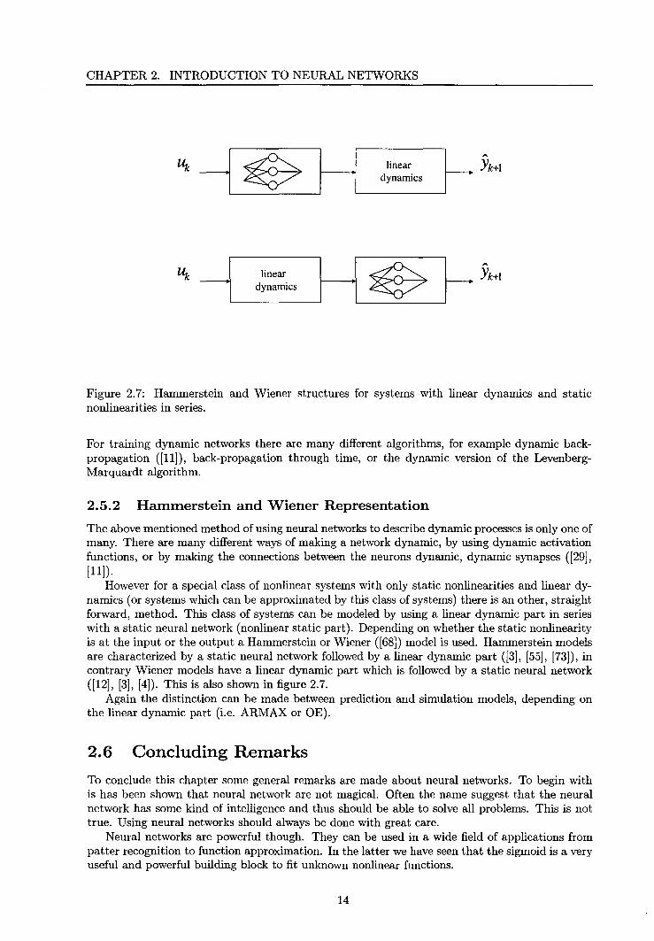
Figure 2. 7: Hammerstein and Wiener structures for systems with linear dynamics and static nonlinearities in series.
For training dynamic networks there are many different algorithms, for example dynamic backpropagation ([11]), back-propagation through time, or the dynamic version of the LevenbergMarquardt algorithm.
2.5.2 Hammerstein and Wiener Representation
The above mentioned method of using neural networks to describe dynamic processes is only one of many. There are many different ways of making a network dynamic, by using dynamic activation functions, or by making the connections between the neurons dynamic, dynamic synapses ([29], [11]).
However for a special class of nonlinear systems with only static nonlinearities and linear dynamics ( or systems which can be approximated by this class of systems) there is an other, straight forward, method. This class of systems can be modeled by using a linear dynamic part in series with a static neural network (nonlinear static part). Depending on whether the static nonlinearity is at the input or the output a Hammerstein or Wiener ([68]) model is used. Hammerstein models are characterized by a static neural network foliowed by a linear dynamic part ([3], [55], [73]), in contrary Wiener models have a linear dynamic part which is foliowed by a static neural network ([12], [3], [4]). This is also shown in figure 2.7.
Again the distinction can be made between prediction and simulation models, depending on the linear dynamic part (i.e. ARMAX or OE).
2.6 Concluding Remarks
To conclude this chapter some general remarks are made about neural networks. To begin with is has been shown that neural network are not magical. Often the name suggest that the neural network has some kind of intelligence and thus should be able to solve all problems. This is not true. Using neural networks should always be done with great care.
Neural networks are powerful though. They can be used in a wide field of applications from patter recognition to function approximation. In the latter we have seen that the sigmoid is a very useful and powerful building block to fit unknown nonlinear functions.
14
2.6. CONCLUDING REMARKS
A disadvantage of neural networks is that they fully rely on the examples shown during training. This makes the experiment design to collect the examples very important and should never be underestimated. Another disadvantage of being fully dependent on examples is that neural networks can not extrapolate.
15
CHAPTER 2. INTRODUCTION TO NEURAL NETWORKS
16
Chapter 3
Hybrid Neural Modeling
3.1 Introduetion
This chapter, together with appendix E, is the result of an extensive literature study on the topic of combining a priori knowledge with neural networks. This chapter is about combining mathematica! models, that describe the process partially, with neural networks, which are used to account for the unknown parts of the process, i.e. hybrid modeling. The neural network itself, however, is still a black-box.
The term hybrid is a much used term which is sometimes used for modeling that combines both time-event and state-event, or for models which have a discrete time part and a continuous time part. Here hybrid means that a neural network is used in combination with a white model. In literature this is sometimes also referred to as grey-box modeling, semi-empirica! modeling or semiparametrie modeling.
This chapter begins with some motivations for hybrid modeling. In section 3.3 the different approaches of hybrid modeling will be discussed that were found in literature. When combining this chapter with appendix E one can formulate a pretty general methodology for using all available prior knowledge about the process and how to develop a hybrid model. A brief formulation will be presented in section 3.4, the complete formulation can be found in appendix E, section E.3.
3.2 Motivations for Hybrid Modeling
Modeling a process can be clone in different ways. Finding a good model of a process can be based on physical insight and prior knowledge of the process. This modeling based on first principles is called white-box modeling. On the other hand if no knowledge about the process is available what so ever, one can chose a model structure from a family of structures, which are flexible and have been proven successful in the past, and try to fit it to the process data (i.e. NARMAX, etc.). This is called black-box modeling. In practice however there usually is some prior knowledge about the process available but there also are some unknown parameters or unknown dynamics present. In this case a combination of white-box and black-box modeling can be used, i.e. grey-box modeling. Grey-box modeling is a much used technique and has benefits of both white-box and black-box modeling (for example [7], [9], [10], [18], [24], [27], [34], [40], [76] ).
Neural networks are a class of black-box models. However incorporating prior knowledge (i.e. grey-modeling, or hybrid modeling) can be beneficia! and can eliminate some of the drawbacks of neural networks. In literature it has been shown that the use of prior knowledge enhances the generalization capabilities of the network, that less data are necessary for parameter estimation, more accurate and consistent predictions are produced and a more reliable extrapolation can be achieved. Moreover network complexity can be reduced. An other advantage of hybrid modeling (over black-box modeling) is that hybrid modeling willlead toa model with a modular structure
17
CHAPTER 3. HYBRJD NEURAL MODELING
prior model
u +" ,/ " y
neural residual
network
Figure 3.1: A neural network parallel with a prior model.
which in turn increases insight in the process ([60]), i.e. each subprocess, depending on the prior knowledge, is modeled by a white-model or a neural network, which tagetherforma model of the whole process.
3.3 Hybrid Modeling
3.3.1 Parallel Structure
When a prior model is available which describes some of the charaderistics of the process this can be used as a backbone for the neural networkin two (obvious) ways. The prior model can either be placed parallel with the neural networkor in series with the neural network (Agarwal [2]). A parallel scheme is given in figure 3.1, and can be written in equations as:
fi= W(u) +N(u,B) (3.1)
with W a prior (or default) model, N the neural network with parameters e, u the inputs and fj the outputs. When a parallel scheme is used, the prior model describes the process pretty well and the neural net is used to account for deviations from the prior model. In addition the default model is often used for providing extrapolation in the area where data are not available.
Thompson and Kramer ([45] and [74]) use this approach for rnadeling a fed-batch penicillin fermentation plant. They use a default model to estimate the states of the system, which is put parallel to a neural network which adjust the states. The inputs for the default state model and the neural network are the states of the system at a previous sample. For the neural part of the model they use a radial basis function network (RBFN). The advantage of the RBFN is that it models the residuals in the domain where data are available and that it gives a negligeable contribution in area where data were not available. So in areas of sparse data the hybrid model relies on the prior (i.e. default) model. This somewhat overcomes the main problem with neural networks, which is that they can not extrapolate. However Su et al. [72] use sigmoid activation functions in their parallel scheme to model a complex polymerization process. They use a first principles model in which simple reaction kinetics are assumed and use a dynamic neural network to capture the model mismatches (i.e. residuals).
18
3.3. HYBRID MODELING
l I u prior z neural
model ------1
network " y
(a)
u neural z prior r-------o
network model " y
(b)
Figure 3.2: A neural network in series with a prior model. (a) Prior model before the neural network; (b) Neural network before the prior model.
3.3.2 Series Structure
When a series scherne is used, as shown in figure 3.2, there are two possibilities (Kernna and Mellicharnp [41]), either the prior model can be used before the neural network (equation 3.2a) or after the neural network (equation 3.2b):
y y
N(W(u), i) W(N(u), i)
(3.2a)
(3.2b)
where u represents the input and i an additional input to the neural network or the prior model which can be used in cases where the second part of the series structure has additional inputs or disturbances next to the output of the first part.
The series structure can be used to describe two different processes in series, one of which is known and the other one unknown, or, when the prior model is placed after the neural network, it can be used to force the output to be consistent with a prior model. In other applications the series structure can be seen as a data-extraction rnethod or as a filter ([41]).
An exarnple is given by Mazak [51], who uses a dynarnic neural network to perforrn a state estirnation and then a static prior model as output model. When in the series scherne of figure 3.2b, both the inputs of the network and the prior model (resp. i and u) are chosen the sarne one gets the scherne of figure 3.3 ([2]). In this scherne the neural network can be used to estirnate an unknown parameter, an unknown function or even unknown dynarnics, of the prior model.
Masri [50], Van Oasterurn [79] and Ploernen [60] use this rnethod for rnadeling mechanica! systerns in which the equations of motion can be derived quite easily (prior model) but in which the friction has an unknown forrn, which in turn is modeled using a static sigrnoid feedforward neural network. Also Psichogios and Ungar [62] use this rnethod in rnadeling a fedbatch bioreactor. They derive a sirnplified modelbasedon rnass balances (prior model) in which the rnicrobial growth rate is the unknown component which is modeled by a static sigrnoid feedforward neural network.
19
CHAPTER 3. HYBRID NEURAL MODELING
neural network
u
A
prior y model
Figure 3.3: A series hybrid model.
3.3.3 Local Model Networks
For many systems adequate models of the system behavior within small operating regimes can be found without too much diffi.culty, while global models, covering all possible operating conditions, tend to be very complex and diffi.cult or expensive to build. When local models are available however a global model can be build by smoothly interpolating between locally valid models ([87]). A local model <I>i will be valid within its particular operating regime, and will be more or less invalid outside this regime. A global model <I> then is formed by the sum of the local models weighted by a validity function Pi :
The validity function Pi (which depends on both the inputs u and the states x) of alocal model <I>i is defined such that it is almost equal to one around the operating regime of <I>i and almost zero outside the operating regime of <I>i. And furthermore:
(3.4)
This way a parallel structure can be formed which resembles a neural network, and especially looks a lot like a radial basis function network (which also forms a global model from local approximations). That is why this method is called local model networks (LMN).
An example is given by Johansen [38], who uses state space models as local models and interpolates between them. Hunt [35] on the other hand uses local ARMAX models. A detailed description is given by Zbikowski et al. [87].
3.4 Hybrid Modeling Approach
The methodology next presented closely follows Thompson and Kramer [74]. At first sight hybrid rnadeling seems to have an 'ad hoc' nature, but this is of course caused
by the fact that each specific process will have its own specific type of prior knowledge available.
20
-------------------------
3.4. HYBRJD MODELING APPROACH
However, from the previous section one can form a guide for designing hybrid models. One can distinguish the following cases:
1) The first-principles model is a default model, which characterizes the process but is not accurate. In this case the default model should be placed parallel with the neural network, which then should be trained to fit the residuals. This can be used for example to model a gas, the default model would be the ideal gas law and the neural net should model deviations from the ideal gas law.
2) The first-principles model describes a process prior to or posterior tosome unknown process. The neural network and the prior model should be placed in series.
3) The first-principles model is a simplified modeland has some unknown parameters or unknown dynamics. In this case the scheme of figure 3.3 should be used. The neural network should be used to describe the unknown part of the prior model. An example is a mechanica! system in which the equations of motion can be deduced, but in which the friction has an unknown form.
4) The first-principles model is alocal model, only valid within a certain operating regime. This local model should be placed parallel with a model which describes the regions where the local model is not valid. Both should be weighted by a validity function. The validity function of the local model should be 1 around its operating regime and almost zero outside it, the other validity function should be zero around the operation point of the local model and about 1 outside that region.
Using this approach models will have a modular structure, and all the prior knowledge available can be used. Compared toa black-box neural network the neural networkin the hybrid model will in general have less parameters and, furthermore, the total hybrid model will be a better system description than a plain black-box neural network.
The schemes in this chapter can be applied to input-output models as well as state space models or other model classes.
21
CHAPTER 3. HYBRlD NEURAL MODELING
22
Chapter 4
Introduetion to MPC
4.1 Introduetion
During the last decade Model Based Control (MBC) has emerged as a powerful control technique, especially in (petro-) chemica! industry. Model Predictive Control (MPC) belongs to the class of model based controllers. The first ideas about MPC emerged in the early 1960's, when Zadeh, Whalen [86] and Propoi [61] started out on linear programming and moving horizonsin time for optimal control purposes. Further work was clone in the 1970's by the application of MPC in the petrochemical industry by Richelet et al. [65] and Cutier and Ramaker [16]. It became clear that the strength of MPC lies in the fact that it can deal with processes which are multi-variabie and have constraints in a very clear way.
In short MPC can be described as a method in which a model of the process that must be controlled is used to predict the future effect of possible changes to that process ([53]). A practical performance criterion is minimized in order to calculate the optimal inputs, bringing the process behavior very near to the preferred behavior. This procedure of finding the optimal control steps for the process by miniruizing a performance criterion is repeated every time a new control move is implemented to the process (e.g. each sampling time of the process).
The following section contains a brief introduetion to (linear) MPC. Inthelast section of this chapter the use of nonlinear MPC is discussed.
4.2 MPC
4.2.1 Outlines of MPC
For the application of MPC a model of the process is necessary. This model is used to calculate the optimal inputs to achieve the desired output. In figure 4.1 the principle of MPC is shown schematically. At the current time sample k, the following cost function is minimized:
(4.1)
in which Yk+l are future outputs of the process predicted using the model of the process, Tk+l the desired outputs (setpoints) of the process for the next p time steps, .ó.uk+l deviations from the previous input, Uk+l-1 (i.e . .ó.uk+l = uk+l- Uk+l-1) and 11-llhr and 1\.1\f.rr the vector norms
y y u 1t
with weighting matrices r~r y and r;;r '" i.e.:
(4.2)
23
CHAPTER 4. INTRODUCTION TO MPC
controlled variabie
manipulated variabie
past future
process MPC-model
control horizon
Figure 4.1: The principle of MPC.
setpoint
The cost function consists of two terms. The first term contains the difference between the desired response and the predicted process output, and this difference is weighted with r y· Each specific output has its own weight associated with it, which makes it possible to weight certain outputs more heavily than others (equation 4.2). The secoud term of the cost function contains the deviation of the manipulated inputs, with weight r u· Notice that not the absolute value of the input, uk+l, is used in the criterium but relative control moves, ~uk+l· An advantage of this is that when the process has the desired trajectory the fust term in the cost function will be zero and the MPC does not changes the inputs anymore, since the cost function will be zero when maintaining to apply the sameinputs (~uk+l = 0).
The model within the MPC prediets the process outputs p samples ahead, and these values are compared to the desired trajectory p samples ahead. This is called the prediction horizon of the controller, which is p samples. The controller has a control horizon of m samples, i.e. the inputs are changed only the first m samples, after which the inputs are kept constant.
This procedure of calculating the optimal inputs is repeated each sample, each time only the first calculated input is actually used as input for the process. Both on the inputs and outputs constraints might be present. While minimizing the cost function these constraints are accounted for. T\ming the MPC is finding the optimum weighting veetors r y and r u and the length of the prediction and control horizon, p and m.
4.2.2 Tuning of MPC
Like a PID controller an MPC controller also has to be tuned. Because the implementation of the controller is usually done using a digital computer a sample time must be chosen. The sample time of the MPC need not be the same as the sample time of the process. The sample interval should be small enough to capture the dynamics of the process, yet large enough to permit on-line optimization of the cost function 4.1.
Tuning an MPC is done by varying the prediction horizon p, control horizon m, and weighting veetors r y and r u until the optimum settings are found. Previous research in the area of model predictive control done by Leenheers [46] , Van der Meulen [81] and Satter [67] has come up with the following rules of thumb:
• The length of the prediction horizon should be longer than the inverse response of the
24
4.2. MPC
system, longer than the dead time of the system and longer than the largest time constant of the system. By increasing the length of the preilietion horizon the controller becomes less aggressive and stability of the controller can he better guarantied.
• The length of the control horizon must be less or equal to the length of the preilietion horizon, a good choice is to take the length of the control horizon between i and ~ of the preilietion horizon. By increasing the control horizon the controller becomes more aggressive and stability of the controller becomes less.
• Outputs with a high weight r y follow the desired trajectory better than outputs with low weights. Increasing the weight of an output makes the controller more aggressive.
• Inputs with low weights r u are used more often than inputs with high weights. The relative values of r u indicate which inputs are used more or which are used less. Decreasing the weight of an input makes the controller more aggressive.
The first rule, which is about the preilietion horizon, is easy to understand. For systems with an inverse response or deadtime the controller can not foresee the exact influence of an alternation of an input when the preilietion horizon is too small. For the same reason the preilietion horizon should also be in the order of the largest time constant for the controller to foresee the final influence of the calculated inputs. The controller will become more aggressive when the prediction horizon is short. The controller then is only able to foresee the short-term influence of a control action and will become more aggressive and apply bigger control moves.
It is proven that unconstrained MPC will he stabiefora preilietion horizon of infinity ([81]), although this does not apply to constraint MPC with a finite preilietion horizon, it can generally he said that stability increases when the preilietion horizon is longer.
The length of the control horizon must at least he one, to implement one control move. Choosing the control horizon beyond the preilietion horizon is not practical. When the control horizon is small, the controller has only a few control moves to achleve the desired goal, in which case the controller will use small control moves, in order to reach that goal. When the control horizon is longer, the controller can use more control moves to achieve the goal, in which case the controller can be more aggressive, because it can compensate for the aggressive control moves it made in the beginning later on.
The weights r u are move penalties for using a certain input. An input with a bigger move penalty will be used less than an input with a smaller move penalty. The same goes for r y, the setpoint penalty. Outputs with a bigger setpoint penalty are punished more when the trajectory is not the desired trajeetory, and will thus follow the desired trajectory closer.
With the setpoint and move penalties r y and r u not the absolute values are important but the values relative to each other. The relative values in r y indicate which output should follow the desired trajeetory most favorite. The relative values in r u indicate which input should be used less, to achleve the desired response. Finally when for example r u is several orders of magnitude smaller than r y the controller will calculate big control moves to follow the desired trajectory. In contrary, when r u is in the order of magnitude of r y the controller might find it more important not to change an input than to achieve the desired setpoint for the outputs.
4.2.3 Open-loop MPC and Closecl-loop MPC
MPC has the nature of a feedforward controller, it calculates the optima! inputs and applies them to the process. However a feedback loop can also he incorporated when the controlled outputs are measured quantities. This feedback loop can then he used to adapt the model within the MPC. This results in two different types of MPC modes which is shown in figure 4.2, in which mk are measured disturbances and nk unmeasured disturbances. When there is no feedback loop present, e.g. when the controlled quantities are not measured on line, the MPC mode is called open-loop. When a feedback loop is present, i.e. the controlled quantities are measured on-line, the MPC
mode is called closecl-loop and the measured outputs, aftersome filtering, can he used to adapt the model within the MPC.
The feedback loop is a very powerful tool to capture model mismatches and can add robustness against model errors. However, the feedback loop generates a closed loop in the control scheme (as the name closecl-loop MPC implies), which, when not properly tuned, can cause instability.
The most common feedback method is to compare the measured outputs of the process with the model prediction at time k to estimate the disturbance dk = Yk- Yk, in which Yk is the process measurement and Yk the model estimate ([30]). In the MPC cost function the disturbance term is then added to the output prediction over the entire prediction horizon, which gives for the cost function of equation 4.1:
(4.3)
This procedure assumes that differences observed between the process output and the model prediction are due to additive step disturbances in the output that persist throughout the prediction horizon. Although simplistic this error model offers several advantages ([30]):
• It approximates slowly varying disturbances. Since errors in the model can appear as slowly varying output disturbances, it provides robustness to model errors.
• It provides a zero offset for step changes in the setpoints.
However the controlled outputs may not always he measured outputs and thus close-loop MPC is not always possible.
4.2.4 Advantages of MPC Compared to Conventional Controllers
MPC has certain distinct advantages ([78], [83]). Most advantages arise from the fact that the controller is model based. First of all MPC is capable of handling interaction between different process parameters. Also inverse response and deadtime can he handled by MPC. Another advantage is that it can suppress both measured and unmeasured disturbances. A very important, and
26
4.3. NONLINEAR MODEL PREDICTIVE CONTROL (NLMPC)
maybe the most important, advantage is that MPC can handle constraints in a very clear way. MPC can also be used to control unmeasured process outputs.
A disadvantage of MPC is, however, that an accurate model of the process is necessary
4.2.5 PRIMACS
The MPC algorithm used is integrated in the PRlMACS software package. PRlMACS is a real time software package developed at TNO-TPD which is used in industrial processes to measure and collect data and to analyze these data which afterwards can be used for model purposes and controller design. It is also possible to filter data or to process data.
The software package consists of a number of different modules, which are independent applications, with each their own task, i.e. signal processing, modeling, data acquisition, and presentation. The PRlMACS software is capable of presenting real time data to the user. While the package is connected to a process or simulation data is send continuously between the PRlMACS database and the I/ 0 module. Recently an MPC module has been developed and has been tested on several cases: fluidized catalytic cracker (Peeters [59]); thermohydrolic example process (Van der Meulen [81], Umans [78]); compressor station (Satter [67]; Leenheers [46]); glass furnace (Wassink [83]).
4.3 Nonlinear Model Predictive Control (nlMPC)
4.3.1 nlMPC in PRIMACS
In the above MPC, although it in principle can be applied to both linear and nonlinear systems, was linear, i.e. a linear model descrihing a linear system and using a linear optimization routine for minimizing the cost function 4.1. Applying MPC toa nonlinear process brings a lot of diffi.culties. First of all an accurate nonlinear model of the process must be available, or must be made, and the nonlinear model must be fast enough for practical optimization, i.e. for the MPC to be used real time. Secoud the minimization problem of the cost function 4.1 becomes nonlinear. This increases the complexity of the optimization problem, and leads to an increase in calculation power needed.
In PRIMACS for nlMPC a campromise is made, in which the model is nonlinear, but the optimization problem is kept linear, saving much processor time ( [71]). The nonlinear model is used to calculate the future response of the system when the current inputs are not changed (~u = 0). The effect of possible control actions is superimposed on this response using a locally linearized model of the nonlinear model. This methad was proposed by Garcia [23] and can be expressed as:
~ ~~u=O ~~u (4 4) Yk+I = Yk+l + Yk+I .
in which Yk+l is the predicted system response, flt.+1° is the predicted system response using the nonlinear model when no further control actions are taken (~u= 0) and fit.+1 is the predicted systems response using the linearized model when control actions ~u are applied.
4.3.2 nlMPC Combined with Neural Networks Described Literature
When using nlMPC one needs an accurate nonlinear model of the process to be controlled. Many different types of nonlinear model classes can be used ( [30]). One can for example use a nonlinear first-principles model, but development of such a model is very complex and difficult or expensive to build.
Neural networks are a class of nonlinear black-box models which have been proven in literature to be very successful to describe nonlinear processes. It thus seems a logical step to use neural network based modelsin nlMPC.
Wassink [83] has written a survey on this topic of using neural networks as nonlinear models for nlMPC. He finds that in many articles neural network based nlMPC is compared with conventional linear controllers such as PID control or linear MPC. From that he draws the condusion that neural network based nlMPC perfarms better than conventional controllers. However another condusion
27
CHAPTER 4. INTRODUCTION TO MPC
he draws is that the method of how to incorporate dynamics in the neural network, used for modeling a nonlinear dynamic system, is still non-trivia!.
28
Chapter 5
ldentification using Wiener N eural Network Models
5.1 Introd uction
Identification of a system (black-box modeling) has an iterative nature. First an experiment has to he designed that excites the system to gain data from the process. After the data have been collected a model representation has to he chosen. Different model representations can he chosen. The choice of representation depends on the application of the model, several different black-box model representations can he used ([80]). Once the model representation is chosen the parameters have to he estimated. And after estimating the parameters the model has to he validated. If the validation shows that the model describes the process well enough, one is finished, if the model does not describe the process well an other model representation must he chosen.
In this chapter the problem of experiment design for a nonlinear system will he discussed and a 2 stage parameter estimation technique for a Wiener neural network model will he presented.
5.2 General System ldentification Approach
Backx [6] has extensively described a way to obtain a model of an industrial process (this is also described by Weetink [84]). The identification of a general industrial process is performed in several well defined steps, each of which gives necessary information about the dynamic and static behavior of the process.
1. Gathering a priori information.
2. Pree run experiment
3. Step-experiment
4. Staircase experiment
5. First PRBS experiment
6. Final PRBS experiment
To get a base for the experiment design the fust thing which has to he clone is to get an indication of several characteristics of the process, the smallest and largest time constant, normal operating points and ranges of inputs and outputs. Process operators may have a good insight to in these cases.
The second phase of the identification protocol consists of the free run experiment. In this experiment the outputs are measured while the inputs are kept at a constant value. This way the
29
CHAPTER 5. IDENTIFICATION USING WIENER NEURAL NETWORK MODELS
noise varianee can he obtained. Eecause a high signal to noise ratio is preferred this experiment can help to determine which inputs and outputs can he used for identification.
The third step consists of step-experiments. The aim of these experiments is to obtain an indication of the gains and a better estimation of the time constants. Step inputs are applied to each input separately.
The fourth phase in the protocol is the staircase experiment. In this experiment staircase-like signals are applied to each input separately. The aim of the staircase experiment is to check for static nonlinearities and the existence of hysteresis. The step amplitude is chosen in such a way that the whole input range is covered.
After the staircase experiment the fust PRES experiment can he done. In this stage independent Pseudo Random Einary Signals (PRES) are applied to all inputs simultaneously. A PRES signal is a signal which is symmetrie around the normal operation points and has a fixed amplitude (e.g. figure 5.1). A PRES signal has a white frequency spectrum (i.e. all frequencies are present with the same energy). The aim of the first PRES experiment is todetermine the bandwidth of the process and to make an estimation of the relative delays by computing the cross-correlation functions of the inputs and outputs.
In the last stage the final PRES experiment is done to obtain the data set from which the initia! model of the process will he estimated. Again mutually independent PRES signals are applied to the inputs simultaneously. The design of this experiment is the most difficult and critica! aspect of the whole procedure. The design parameters are the parameters of the input signals (amplitude, bandwidth) and the duration of the experiment.
5.3 Experiment Design for Nonlinear Systems
5.3.1 PRBS for Linear Systems
Experiment design is a very important step in the identification procedure. The identification experiments determine the final validity and accuracy of the model.
An important factor is the degree of persistenee of excitation of the input signal (i.e. the maximum number of parameters that can he estimated with the signal [80]). This degree should he sufficiently high with respect to the number of parameters to he estimated. In this respect a Zero Mean White Noise signal is the ideal input since it is persistently exciting of any order. However although the white noise is a niceinput signal from a theoretica! point of view, for most systems it is notallowed to apply such a signal, especially because of the high-frequency excitation. More over since processes often are low pass filters there is no use in putting a lot of energy in the high frequency region.
An input signal that is easy to design is a Pseudo Random Einary Sequence (PRES). A PRES switches at distinct time intervals between two values (usually -1 and 1) with a probability of a half. An example is shown in figure 5.1.
5.3.2 Identification Signal for MIMO Nonlinear Systems: QPRTS
For nonlinear systems experiment design is more complicated than for linear systems. Linear systems obey the principle of superposition and it is sufficient when the identification experiment has a fixed amplitude. However for a nonlinear system the principle of super position does not hold, and a twice as large input need not have twice the effect of the original input. So for identifying nonlinear systems one also needs to change the amplitude of the signal. Eouman [11] describes a much used random signal which has the same appearance as the PRES but has a random amplitude (a discrete form of white noise, figure 5.1). He compares the preilietion capability of two dynamic neural networks of which one was trained on data retrieved from a PRES experiment and one which was trained on data retrieved from an experiments with a PRES with random amplitude. He finds that the latter neural network performs far better than the fust.
Figure 5.1: A PRBS signa! and a PRBS signal with a random amplitude.
However although the amplitude is varied the switching time of the signa! is still fixed. Therefore the switching time must he chosen with great care. When the switching time is too long only the slow dynamics of the system will he excited. In contrary when the switching time is short only the fast dynamics will he excited, and the system may act as a high-pass filter.
All this considered one can conclude that an experiment used to identify a nonlinear process should (at least) meet the following demands:
• The process dynamics must he excited sufficiently. For linear processes this can he clone with a PRBS experiment. However in nonlinear systems the dynamics may differ from one operating point to another and one should consider the whole operating regime.
• Statics should also he included in the experiment. When for a linear system the amplitude of the input increases by a factor of two, the amplitude of the output also increases by a factor of two, because the static gain is the same for the whole system. For nonlinear systems this does not hold. The static gain may differ in different operating regimes.
• When the system has multiple inputs and multiple outputs (MIMO) it does not suffice looking solely at the response of the system when the inputs are changed successively, it is also necessary to look at the hehavior of the system when several inputs are changed at the same time (in contrary to linear systems in which it is suflident to look at the inputs independently since the effects are additional).
One way of looking at the problem of experiment design for identification of a nonlinear system is that the experiment should slowly cross through the whole operating regime of the plant and at the same time excite the local dynamics. One might think of a slow sine with a small PRBS added. This would slowly cross the whole operating regime and excite the local dynamics. This might work for a system with only one input. However the input always changes only a little step
31
CHAPTER 5. IDENTIFICATION USING WIENER NEURAL NETWORK MODELS
A QPRTS signal which is a sum of three PATS signals
~ _: 0 500 1 000 1500 2000 2500 3000
~ -~ 0 500 1 000 1500 2000 2500 3000
~ -~~ ; tlJ;I?QUj 0 500 1 000 1500 2000 2500 3000
i_: 0 500 1 000 1500 2000 2500 3000
sample
Figure 5.2: An example of a QPRTS signal.
and because of the nonlinearity of the system a small step might give a totally different ( dynamic) response compared to a large step. Another problem is when the system has multiple inputs and multiple outputs (MIMO). Applying sine like inputs toeach input at the sametime would give Lissajous like figures in the input space, which most likely do not cover the whole operating regime of the system.
One might circumvent all the problems discussed above by using a Quantisized Pseudo Random Trinary Sequence (QPRTS). A QPRTS has the charaderistics of a PRBS, and is the sum of a couple of Pseudo Random Trinary Sequences (PRTS). An example of a QPRTS signal which is the sum of three PRTS is shown in figure 5.2. A PRTS switches between -1, 0 and +1 the same as a PRBS switches between -1 and 1. A QPRTS is build from a number of PRTS with a different amplitude and a different frequency. Usually a PRTS with a bigger time constant has a bigger amplitude. The idea behind the signal is that the relatively fast PRTS with a small amplitude is used to excite local dynamics while the relatively slow PRTS with a big amplitude is used to push the system through the systems whole operating regime. The random character has the advantage that it can also be used for MIMO nonlinear systems. Also because of the presents of big amplitude changes in the signal, not only small input deviations are accounted for but also large deviations occur. From the basic idea (slow signals with a big amplitude to move across the operating regime of the plant, faster signals with a smaller amplitude to capture local dynamics), one can come up with some rules of thumb to design a QPRTS experiment:
• Choose the time constant of the signal with the biggest amplitude in the order of the settling time of the system, and the amplitude so that it covers the whole input range.
• Choose the time constant of the signal with the smallest amplitude the same as the time constant which would be used for the PRBS experiment for linear identification. Also choose the amplitude the same as would be done for linear identification.
32
5.4. WIENER NEURAL NETWORK MODEL
• Choose all other time constauts and amplitudes in between the two above.
Oasterurn [79] has done some experiments with this signal and compared it with the excitation of a system by white noise or PRBS. She found that the QPRTS excites the process more than the other signals. The advantage of the QPRTS signal above a white noise signal is that it really pushes the system around in the operating regime of the plant, while a random (noise) signaloften changes too fast to really move around in the operating regime of the system.
As discussed above for nonlinear systems it is really important to have a experiment which covers the whole operating regime of the nonlinear system.
A disadvantage of the QPRTS signal is that it might not always be possible to use on a real system. Especially for example on chemica! plants. The fact that the signal really excites the whole process will be a nightmare of every operator.
5.4 Wiener Neural Network Model
5.4.1 Wiener Neural Network Model Structure
A subclass of hybrid models in the class of hybrid series models is formed by models which consist of a linear dynamic model and a static neural network in series. This class of models can be used to describe processes with static nonlinearities. Depending on whether the nonlinearity is a static input nonlinearity or a static output nonlinearity, the neural network can either be placed befare or after the linear dynamic model. In literature these kind of models with a static nonlinearity and linear dynamics in series are often referred to as Hammerstein models, in case of an input nonlinearity (for example [3],[73]), or Wiener models, in case of an output nonlinearity (for example [4]). A Hammerstein type of modelfora fust order single-input-single--output (SISO) system would be of the following form:
z
z
(5.1)
(5.2)
in which NH(u) is a nonlinear function of u (accounted for by a neural network), and T is the time constant of the system. In contrary a Wiener type of model would be of the form:
rz+z y
u
Nw(z)
(5.3)
(5.4)
in which Nw(z) is a nonlinear function (neural network) of z. Notice that in practice z is not measurable, it is only used here to demonstrate the model structure.
Many industrial processes can be modeled, or can he approximated well enough, by a Hammerstein or Wiener type of nonlinear model. In chemica! processes for example static nonlinearities appear as nonlinear valves, nonlinear actuators and nonlinear sensors. In communications static nonlinearities are used to model nonlinear filters, nonlinear channels, and nonlinear amplifiers. In mechanica! systems static nonlinearities can be used to model backlash and friction.
A typical Wiener neural network model structure is shown in figure 5.3. Notice that the static gain of the linear dynamic part can be absorbed in the static neural network, and thus the static gain of the linear dynamic part can be chosen freely, i.e. 1 in the picture.
5.4.2 A 2 Stage Approach for Parameter Estimation of the Wiener Neural Network Model Structure
A QPRTS experiment can be used to collect data from a nonlinear system which then can be used to estimate the parameters of a nonlinear model, for example the Wiener neural network model.
33
CHAPTER 5. IDENTIFICATION USING WIENER NEURAL NETWORK MODELS
u linear z neural -o dynamics network
y
u 1 z
neural -o --r s+l network
y
Figure 5.3: A Wiener neural network model structure.
However as has been pointed out the QPRTS is not a very practical signal, which for example can not be used on chemica! plants.
For the Wiener neural network model one can estimate the parameters (i.e. the time constauts of the linear dynamic part and the parameters of the neural network) using experiments that does not need to drive the process out of the normal operating regime.
The fact that the static gain in the linear dynamic part of the Wiener model structure can be chosen freely can be exploited. Choosing the static gain 1 as in figure 5.3 causes the linear dynamic part to have no contribution when the process runs in steady state, its gain is simply 1 which in turn causes z to be equal touwhen the process runs in steady state. Notice that while z was in practice not measurable, z now can be reconstructed for steady state data. This is a very important property because now the parameters of the neural network can be estimated using only steady state data.
Once the parameters of the neural network are estimated the linear dynamic part of the model can easily be estimated using linear identification techniques (e.g. by a PRBS experiment ). A small amplitude should be used to keep the system in a linear region. When the linear dynamic part is found one should choose the static gain equal to unity, since the gain is already accounted for by the neural network.
The parameters of the Wiener neural network model structure eau thus be estimated in 2 stages:
1. Estimate the parameters of the neural network using steady state data of the system.
2. Estimate the linear dynamic part of the model structure using plain linear identification techniques.
5.4.3 Concluding Remarks
The Wiener model structure and the estimation approach has several advantages and disadvantages. An advantage is that the difficulty of experiment design for the nonlinear system is reduced to the experiment design problem for a linear system. Another advantage is that the model will be very accurate (permitted that the processcan bedescribed by a Wiener neural model) because the neural network partand the linear dynamic part are estimated separately making the parameter
34
5.4. WIENER NEURAL NETWORK MODEL
estimation optimization easier. A disadvantages is that it cannot cope with nonlinear dynamic behavior.
35
CHAPTER 5. IDENTIFICATION USING WIENER NEURAL NETWORK MODELS
36
Chapter 6
The Copolymerization Process
6.1 Introduetion
This chapter is an introduetion to the case study. Polymers and polymerization processes are explained and also the case study, a copolymerization process of polyethylene in a loop reactor, is discussed. The final goal is to control the polymer properties of the polymer produced and the control problem related to this, and the application of MPC, is also discussed
6.2 Introduetion to Polymers
6.2.1 Polymers and Polyethylene
Polymers are used is a wide range of materials such as plastics, synthetic fibers, rubbers and coatings. The diversity of these polymers is known from common usage as 'nylons', 'vinyl', 'rubber', 'polyesters' and 'acrylics'.
A polymer is an organic molecule which means that it is build up mainly from carbon and hydrogen atoms. A polymer is, as the name implies, a chain of monomers. The monomer is the building block of the polymer. Polymers are usually formed of monomers which have a double bound. The double bound breaks open to form the polymer. For example polyethylene is formed from ethene:
CH2 = CH2 ethene building block
polyethylene CH3- CH2- CH2- ... - CH2- CH2- CH3
A polymer need not be built from one single type of monomer, often a small fraction of an other type of monomer is added, this monomer is then called comonomer. Inserting a comonomer can lead to branched structures, as in figure 6.1, which affects the density of the polymer. For polyethylene a classification, based on density, can be made in three different types of polymer: linear low density polyethylene (lldpe), low density polyethylene (ldpe) and high density polyethylene (hdpe). In table 6.1 an overview of the different types of polyethylene and the density is given.
type of polyethylene density range lldpe (linear low density polyethylene) 0.880 gjcm;:s - 0.950 gjcm;:s ldpe (low density polyehtylene) 0.910 gjcm;:s- 0.940 gjcm;:s hdpe (high density polyethylene) 0.940 gjcm;:s - 0.980 gjcm;:s
Table 6.1: Different types of polyehtylene (Ray [63]).
37
CHAPTER 6. THE COPOLYMER1ZATION PROCESS
4__" LLDPE _/J
LDPE
Figure 6.1: Branching in polymers.
6.2.2 Polymer Properties: Density, MWD and Melt Index
Different polymers are characterized by the type of (co )monomers, density (see previous section) and average chain length (i.e. the average number of monoroers which forma polymer chain).
Polymers will in general not have the same chain length. There is a distribution in chain length Pi, with Pi the molar concentration of species with length i (iE N), figure 6.2. This distribution can approximately bedescribed by the momentsof that distribution. The kth moment, f.Lk, of the chain length distribution is defined by:
CX)
f.Lk =Lik Pi i=l
(6.1)
Especially important are the zeroth moment f.Lo, which can be interpreted as the total amount of polymer, and the first moment f.Ll, which can be interpreted as the tot al concentration of monomer units in the polymer. These moments can be used to calculate the number average chain length Mn and weight average chain length Mw:
CX)
2:: i 2 pi i=l
CX)
2:: iPi i=l
(6.2)
(6.3)
Figure 6.2 shows a typical chain length distribution. The number- and weight average chain length are also displayed in the figure.
An equivalent alternative to the chain length distribution is the molecular weight distribution, MWD. Often it is a good approximation to say that the mass of a polymer build up from i monoroers is equal to i times the mass of the monomer. The molecular weight distri bution Wi can then be defined as:
with mm the molar mass of a monomer and Pi the chain length distrihution (figure 6.3). Also the numher- and weight average molecular weights, M;: and M;:;, can he calculated in the same way as the numher- and weight average chain length, using the moments of the molecular weight distrihution J.L'k:
00
L)imm)kPi (6.5a) i=l 00 00
"2:::: immPi I: wi J.L! i=l i=l
00 00 J.Lo I: pi I: pi (6.5h)
i=l i=l 00
"2:::: immWi J.L2 i=l
00 J.L! I: wi (6.5c)
i=l
The molecular weight distrihution of a polymer is the most fundamental way of characterizing a polymer population. When the molecular weight distrihution is known, other properties can he derived. The molecular weight distrihution has a great influence on flow (or rheological) properties and in the related mechanica! properties it is important for end use.
One of the most familiar flow property is viscosity, which is important hoth in the processing of the polymer and in some end uses. The usual hehavior is that the viscosity decreases with chain length. For polyethylene the logarithm of the viscosity has a linear dependenee of the logarithm of the molecular weight ([22]).
A measure for the average molecular weight and the width of the molecular weight distri hution is the melt index (MI), also called melt flow index. The melt index is measured hy the rate of extrusion of a molten polymer through a capillary of a certain length and diameter, the melt heing supplied from a cylinder hy the weight of a piston. The melt index of a particular polymer is the amount of polymer extruded in a given time, at specified temperature and mass of the piston, and is thus inversely related to the average molecular weight. The test has its favor for simplicity, a relatively short measurement time and the possihility of heing implemented on-line.
39
CHAPTER 6. THE COPOLYMERJZATION PROCESS
Molecular weight distribution 3500
3000
2500
2000
~
1500
1000
500
0 0 5 10
molecular weight
Figure 6.3: Molecular weight distribution.
15
x 104
The characterization is not unique (polymers of different distributions may have the same melt index), but that complication may he unimportant if one can he certain that misleading factors, such as branching, are prohibited. The melt index h of a polymer is defined as the amount of polymer mass in grams that flows through an ortifice of 0.0825 inch in diameter in 10 minutes, at 190° C with 2.16 kg of weight as driving force. Todetermine I10, a driving force of 10 kg is used. The I10/I2 ratio is a measure for the polydispersity of the polymer.
6.3 The Polymerization Process
6.3.1 Reaction Kinetics
There are many different types of polymerization reactions, the stuclied process is a solution polymerization with the use of a Ziegler Natta catalyst. The use of this type of catalyst allows the formation of linear polymers, through the addition mechanism of alpha-olefins at an active catalyst site. The catalyst is a mixture of metal alkyls and transition metal salts ([14]).
In a Ziegler Natta polymerization system a polymer chain is formed by addition of a monomer or comonomer to an existing chain, in random order (figure 6.4 ). This processis assumed to he independent of chain length, i.e. molecular weight. The ra te at which the different (co )monomer units are inserted is determined by the temperature and component concentration.
Growing of the polymer chain can he stopped by several termination reactions, which are also assumed to he independent of molecular weight. Hydrogen for example can he used for chain terminator, but also the (co )monomers themselves can cause chain termination.
Because of the random character of this process, a distri bution of polymer weight is produced. The overall polymer properties of the bulk are determined by the molecular weight distri bution of the polymer phase.
Different solvents can he used, in the range from 1-pentane to 1-decane. A link can he made between the polymer properties and the kinetics:
high meltindex => low molecular weight
=> short chains
=> low viscosity
40
0 catalyst carrier ~ active catalyst site 0 deactivated catalyst site
""-" monomer ")- comonomer
• hydrogen
6.3. THE POLYMERJZATION PROCESS
Figure 6.4: Formation of polymer at a catalyst site.
=} soft polymer
=} high hydrogen incorporation
=} high reaction temperature
=} high chain termination rate
high density =} low comonomer incorporation
=} less branching
=} dense packing of chains
6.3.2 Reactor Description
A polymer plant can be subdivided in several different sections, areaction section, a devolatilisation section, a product handling section and solvent recovery section. The heart of the process is the reaction section where the actual polymer is formed, and for further study only this section will be considered. In this process the polymer is formed in a continuous process. The reactor is schematically shown in tigure 6.5 (a more detailed description can be found in appendix A). The reactor is a loop reactor of the Phillips type (Encyclopedia of polymer science and engineering [49]). Inputs to the reactor are monomer, comonomer, catalyst and hydrogen. The monomers and hydrogen enter the reactor in a solvent, which is used to remove heat from the reaction and to keep the polymer formed in solution. The temperature of the reactor can be controlled by the cooling jackets and the pressure in the reactor is kept constant. The solution is pumped through the loop of the reactor many times compared to the total feed through the reactor to improve mixing, i.e. the recycle ratio is high.
All together there are eight inputs of the process which can be used for control purposes. However because the catalyst feed is already controlled the inputs which might be used as controlled variables by the MPC are hydrogen, monomer and comonomer concentration in the feed, reactor temperature, conversion setpoint, recycle ratio and total feed.
41
CHAPTER 6. THE COPOLYMERJZATION PROCESS
Catalyst
coolant
Feed monomer comonomer hydrogen
coolant
Pump
Effluent polymer
Figure 6.5: The loop reactor (Encyclopedia of polymer science and engineering [49]).
6.4 Control Problem
6.4.1 Control Objectives
The main control objective is direct polymer property control, i.e. melt index and density, during grade changes. An advantage of direct property control is that faster and more complex grade changes become possible. Direct property control also can he used to give setpoint advises for new products. Another advantage is that, because the plant is more flexible in reacting to short term demands, there will he a reduction in product stock. However direct property control is not straight forward because the polymer properties are not measured on-line and the process is strongly nonlinear and has strong interactions.
The main control variables which determine the polymer properties are:
• catalyst concentration
• morromer concentration
• morromer / comonomer ratio
• reaction temperature
• hydragen concentration
The pressure in the reactor mainly effects the solubility of the (co )monomers in the solvent. The primary goal of cantrolling the ( unmeasured) polymer properties can he divided in three
practical control objectives:
1. Polymer property control during grade changes.
42
Hydrogen
Monoroer
Comonomer
Feed
Pump speed
Conversion
Temperature
I! lil
p r 0
c e s
6.4. CONTROL PROBLEM
1---Polymer meltindex density
1----.-- Monomer
1--+-- Comonomer i!! Ij i !, ! 1 I' s i i.ll • ................ ·---~:~·~:-;----~ Reactor ~mperature
Figure 6.6: Controlloops for conversion and temperature controL
2. Increasing production, i.e. increasing the total feed to the reactor, while maintaining to produce the same grade (i.e. polymer with the same melt index and density).
3. Anticipate on a sudden decrease in catalyst efficiency ( distur bance rejection).
In all cases the aim is to control the melt index and density at an accuracy of about 2%. Furthermore there are constraints on the process which should not be violated. There are the
usual constraints on the inputs, i.e. inputs have minimum values (valve closed) and maximurn values (valve fully open) and move constraints, but there is also a process constraint with respect to the coolant temperature. The coolant temperature should not be too low compared to the reactor temperature, because when the coolant temperature is too low the polymer will crystallize at the inner surface of the tubes.
Surnmarized the constraints are as follows:
1. The inputs have ( operating regime dependent) minimum and maximum values.
2. The difference in temperature between the reactor and the coolant should be suffi.ciently low, to prevent crystallization of polymer at the surface of the tubes.
6.4.2 Current Control of the Process
There are a few controlloops present in the reactor of which two are particularly important. Figure 6.6 gives a simplified overview of the process, the inputs, outputs and the two control loops. One of the controlloops involves the reactor temperature. The coolant temperature is controlled such that the reactor maintains at the desired temperature. The other control loop is for the catalyst feed. The amount of catalyst added to the reactor is dependent of the amount of monomers which enter the reactor, temperature and the conversion setpoint. The desired conversion of monomer is given by the desired monomer concentration in the effluent, this value is used by the catalyst controller to adjust the catalyst feed. The catalyst controller is very important because it stahilizes the process.
Currently there is no direct control of the polymer properties. Grade changes are made by applying the new steady state inputs. To speed up the grade change the recycle ratio of the reactor
43
CHAPTER 6. THE COPOLYMERJZATION PROCESS
can he lowered, to achieve that the reactor will behave more like a plug flow and mixing of the different grades will he less ([20]).
However, large grade changes are avoided because they are diffi.cwt (because of the nonlinearities and interactions in the process) and time consuming. For this reasou product schedwing is applied.
6.4.3 MPC of Polymerization Processes Described in Literature
The control problem, having a strongly nonlinear process with many interactions and with constraints, asks for a well suited controller. A nonlinear model predictive controller seems to he suited for this job. In the last few years MPC has become very popwar and good results have been achieved. One of the reasans for it popularity is its success in chemica! processes. In literature many studiescan he found in which MPC was applied (for example [81],[58]).
The use of MPC for direct property control in complex polymerization processes is described less frequently in literature. There are some cases described in literature using MPC to control for example the temperature in an unstable process. Although the temperature can he used to control the polymer properties this is not a direct method.
An example is given by Berber et al. [8]. They use nonlinear MPC to control the temperature of a low density polyethylene (ldpe) reactor, and conclude, based on the simwation reswts, that the reactor temperature can effectively he regulated meeting hard constraints on control inputs over a wide range of operation conditions. They also conclude that the nlMPC performs better than PID control, especially for setpoint tracking.
An other example is given by Gobin et al. [26] who control the temperature of a open-loop unstable train of polymerization reactors, using linear MPC. From their simwations, based on a Speed-Up model of the plant, they conclude that with the use of MPC faster setpoint changes are possible as compared to PID controL However, they also stress that it is diffi.cult to control a nonlinear system with a linearized model away from the linearization point. Furthermore they conclude that the constraint handling capability of MPC is very beneficia!, while PID control aften has to he detuned to cope with constraints. Hidalgo et al. [31] use nonlinear MPC, in a simulation environment, to control the temperature of a polymerization process, however this time to control the process at an unstable operation point.
Cases in which MPC was used for direct property control are for example De Wolf et al. [19] and Kooijmans [44]. De Wolf et al. [19] use linear closecl-loop MPC to control the melt index of polypropylene in a slurry reactor, using a Speed-Up simwation model of the plant. They find that the use of MPC shows significantly better performance both at grade changes and disturbance rejection, which reduces the amount of off-spec production compared to the conventional PID controL Kooijmans [44] uses linear closecl-loop MPC to control the melt index of a polymerization process in a tubular reactor. He compares the simwated MPC results of a grade change with operator control and PID controL He also finds that MPC is superior to both. Saldivar et al. [66] apply nonlinear MPC to control both the molecular weight distri bution and copolymer composition of a semi continuous emulsion copolymerization. Their condusion is that nlMPC shows excellent performance in handling disturbances, under the assumption that the states of the process can he estimated on-line.
Also, literature on direct polymer property control can he found in which other control techniques are applied: Congalidis et al. [15] use conventional feedforward and feedback control to control molecular weight and copolymer composition; Semino et al. [69] use an extended Kalman filter to estimate the polymer properties, which then can he used by PI controllers; Gentric et al. [25] use geometrie control to control the polymer properties of an emwsion polymerization reactor, geometrie control is a model based control algorithm, based on differential geometry.
Umans [78] has clone a feasibility study on the application of model predictive control of the polymerization process under consideration. He stuclied a thermohydrolic process which has the same control problems (strong interaction, input constraints, output constraints) and control objectives ( control of unmeasured variables, disturbance rejection) as the polymerization process.
44
6.5. IMPLEMENTATION OF THE PROCESSIN GPROMS
From this he draws the condusion that MPC should be suited for cantrolling the polymerization process when a good model of the process is available.
6.5 lmplementation of the Process in gPROMS
In the research described in this thesis insteadof real plant data a rigarous first-principles simulation model, developed by J.W. Verwijs from the Process Development & Control Department of DOW Benelux NV, was used to ruimie the plant. The complex simulation program was developed in the gPROMS software package [57] and represents the continuous copolymerization process. The gPROMS model is a very complex model, in which each part of the plant is modeled separately. By connecting the different parts a distributed model is formed with over twentyfourhundred variables and more than thousand internal states, leading to a nonlinear first-principles model of the plant. In all identification and control simulations this rigarous simulation model of the plant was used as being the plant.
The gPROMS model runs on a VMS workstation and is connected with PRIMACS, which runs on a PC, via the External Data Interface of gPROMS. This way real time data communication is achieved between PRIMACS and the gPROMS model which makes it possible to control the gPROMS process, and to collect data, from within PRIMACS. These data can then easily be exported to Matlab, for data processing or rnadeling purposes.
The aim is to use the MPC module of PRIMACS to control the gPROMS process.
45
CHAPTER 6. THE COPOLYMERJZATION PROCESS
46
Chapter 7
Modeling and Control of the Copolymerization Process
7.1 Application of nlMPC to the Polymerization Process
As mentioned in the previous chapter it can be concluded that MPC should be suited to control the polymerization process. The implementation of MPC to control a process consist of several steps ( [77]). At fust an accurate model of the process is necessary, and because the polymerization processis highly nonlinear an accurate nonlinear model has to be developed. This nonlinear model may be a first-principles modelor a black-box model. However developing a first-principles model of the process is difficult and time consuming, but on the other hand identification of a nonlinear model requires very much effort in designing an experiment for estimating the parameters of the black-box model ( chapter 5). Moreover because the controlled variables, the polymer properties, are not measured on-line, which means that the model must be very accurate because it will be used in an open-loop MPC control scheme. The difficulties of first-principles modeling and the experiment design for identification can be overcome by the development of a hybrid model, combining both prior knowledge and a black-box model ( chapter 3). Furthermore one should keep in mind that the model of the process will be used in an MPC controller, which requires that the model must be fast enough for practical optimization.
After a (hybrid) nonlinear model of the process is developed it should be validated on plant data, preferabie by plant data which were retrieved from a specially designed experiment to excite the process as much as possible. Notice that in principle the validation experiment should be of the same nature as the experiment used for black-box modeling. However the number of data necessary is far less than for black-box modeling or parameter estimation. In addition one may be less stringent about the validation data, since no actual modeling is clone.
Finally when an accurate nonlinear model of the process is available and it is implemented in the MPC tagether with the constraints, the MPC should be tuned (chapter 4), the sample frequency of the MPC, length of the prediction and control horizon and weights of setpoint and move penalties should be chosen with care to achleve the desired performance of the controller.
All these different stages were applied to the polymerization process, and the result are presented below. For confidential reasans all quantities are scaled between -1 and +1.
7.2 First Identification Experiments
7.2.1 Step Responses
The first steps in identifying a process are gathering a priori information and looking at some free run experiments (chapter 5). The next step is toperfarm step response experiments. Step inputs were applied to the hydragen and (co )monomer concentration in the reactor feed. The response
47
CHAPTER 7. MODELING AND CONTROL OF THE COPOLYMERIZATION PROCESS
~ c:
0.4
)(
" ~0.3 = ~
-0.336
~ ·0.337
-0.338
0
Step on hydrogen
100 200 300 400 sample
100 400 sample
(a)
Step on comonomer
·0.61.---~--~--~--...,
-0.62
i :;;;-0.63 "' E
100 200 300 400 sample
0.8
0.7
~0.6 ïii c:
" "0.5
0.3 0 100 200 300 400
sample
(b)
Figure 7.1: Step responses of the process. (a) Step on the hydragen concentration in the feed; (b) Step in the comonomer concentration in the feed.
of the melt index and density on these step inputs on both hydragen and comonomer are shown in figure 7.1. From these figures a first estimation can be done for the important time constauts of the process. It can be seen that response on a change of comonomer is faster than a change of hydrogen. The settling time for a step on hydragen is about 300 samples, while the settling time for a step in the cornonomer concentration is about 200 samples. It can also be seen that a step on the hydragen concentration has much more infiuence on the melt index than on the density, in contrary a step on the comonomer concentration has more influence on the density.
7.2.2 Hystereses Check and Steady State Behavior
The next identification step is the staircase experiment. Staircase-like input signals were successively applied to the different inputs, i.e. hydrogen, monomer and comonomer concentration in the feed, reactor temperature, conversion setpoint, total feed and recycle ratio. The results of these experiments can be found in appendix B. It is important though to notice that each time only one input was changed, which does not give inforrnation about what would happen when two or more inputs would be changed simultaneously, because of the nonlinear nature of the process. From the staircase experiments it can be concluded though, that no hysteresis is present in the process.
Another aim of the staircase experiment is to check for the presents of static nonlinearities. In figure 7.2 the static gains of the melt index and density are shown for each of the seven inputs, relative to each other. From the figures it is clear that hydrogen, the temperature and conversion have a lot of infiuence on the melt index, and that the influence of monomer, comonomer, total
hydragen monomer comonomer temperature feed recycle conversion
Figure 7.2: Steady state gains.
feed and recycle ratio is less. The influence of hydrogen on the melt index can he explained by the fact that hydrogen is a chain terminator. The influence of the temperature and conversion are both caused by their impact on the catalyst concentration. At higher temperatures the catalyst will deactivate faster. The little influence of monomer, comonomer, total feed and recycle ratio on the melt index is again caused by the catalyst controller, which will compensate for higher (co )monomer concentrations, feed and recycle ratio to keep track of the desired conversion.
Figure 7.2 shows that the (co)monomer concentration and conversion setpoint have big influence on the density. This was to he expected because the density of the polymer largely depends on the monomer / comonomer ratio.
From the steady state behavior, and the knowledge about the process, it seems logical to take hydrogen and comonomer as the manipulated inputs for a fust control scheme, because the two inputs have a large impact on the melt index and density and because the two inputs are most decoupled.
7.3 General White-Box Modeling of the Reactor
7.3.1 A CSTR as a Basic Unit
From the previous section it can he concluded that hydrogen and comonomer are the important inputs which can he used to control the melt index and density of the polymer. In addition the total feed to the reactor also is an important input since it is part of a control objective ( Chapter 6). The next step in MPC control involves developing a model of the process with hydrogen, comonomer concentration and total feed as inputs, and the melt index and polymer density as outputs.
The first step in modeling the process is to assume certain reaction kinetics. However because
49
CHAPTER 7. MODELING AND CONTROL OF THE COPOLYMERIZATION PROCESS
the exact reaction kinetics are unknown, the model should not rely too heavily on the assumed kinetics. Also a reactor model has to be chosen. Several ideal reactor models are available, such as a plug flow reactor (PFR) or a continuous stirred tank reactor (CSTR), which can he put in series to model non-ideal behavior. The choice between a PFR and CSTR model can be based on impulse or step responses of the process ([42], [48]). The step responses of anideal PFR and CSTR are shown in figure 7.3. Camparing this with the step responses of the process, shown in figure 7.1 of the previous section, it can be concluded that the use of a CSTR model is preferred. This can be understood by the fact that when the recycle ratio of the loop reactor goes to infinity it will become a perfectly mixed reactor, a CSTR ([85]).
Full derivation of the reactor model can be found in appendix C, the final results are presented next.
7.3.2 Mass Balances of Components
The continuous process is modeled using a Continuous Stirred Tank reactor (CSTR) in which perfect mixing is assumed. The volume of the reactor is constant, and it is also assumed that the density of the mixture in the reactor is constant ( since the polymerization takes place in a salution the overall density will mainly be determined by the solution). The model accounts for the hydrogen, monomer and comonomer concentratien in the feed, total feed, hydrogen, monomer, comonomer and live (reactive) and dead (not reactive) polymer concentratien in the reactor, hydrogen, monomer, comonomer and dead polymer concentratien in the effluent and the polymer properties melt index and density, figure 7.4.
The reaction equations are taken from Cavelaars [14]:
Initiation:
* riA MA + Jcat ~ P1,0
M I * r;,B P, B + cat ---+ 0,1
Propagation:
50
(7.1)
(7.2)
(7.3)
F
Terrnination
7.3. GENERAL WHITE-BOX MODELING OF THE REACTOR
F
Figure 7.4: The CSTR model.
(7.4)
(7.5)
(7.6)
in which I~at is an active free catalyst site, MA monomer, MB comonomer, Prn,n a live polyrner chain with m units of monomer and n units of comonomer, Drn,n a dead polymer chain with m units of monomer and n units of comonomer, and r the different reaction rates.
The process main dynarnics can he described through mass balances for (co )monomers (CA and CB), hydrogen (CH) and the momentsof the molecular weight distribution (J-Lk'). The thermal balance is neglected since the temperature of the reactor is kept constant by the cooling jacket. Using the long chain approximation (Ray [64]), the mass balances for (co)monomers and hydrogen are:
dCA F dt v(CA,in- CA)+ RA (7.7)
dCB F dt v(CB,in- CB) +RB (7.8)
dCH F (7.9)
dt v(CH,in- CH) +RH
in which F is the total flow, V the (constant) volurne of the reactor, CA,in, CB,in, CH,in, the concentrations monomer, comonomer and hydrogen in the feed, CA, C B, C H, the concentrations monomer, comonomer and hydrogen in the reactor ( and effluent) and Rx the overall reaction rates of product x:
RA -kp,ACPCA (7.10)
RB -kp,BCPCB (7.11)
RH -kt,HCPCH (7.12)
51
CHAPTER 7. MODELING AND CONTROL OF THE COPOLYMERJZATION PROCESS
with Cp the total concentration living polymer and kp,A, kp,B, kt,H the (temperature dependent) reaction rate constauts for resp. propagation with monomer, propagation with comonomer and termination with hydrogen.
7.3.3 Momentsof the Molecular Weight Distribution
The kth moment, f-Lk', of the molecular weight distribution fora copolymer is defined as ([22]):
00 00
f-Lk = LL(imA+ims)kPi,j (7.13) i=l j=l
with Pi,j the chain length distribution for copolymers with i units of monomer and j units of comonomer. The zeroth and fust moment are important because they can be used to calculate the average molecular weight which is important for the melt index. The moments of the chain length distribution can be derived using the tendency model (Villermaux et al. [82]) from which follows:
dp0 F w
dt + vf-Lo dp'{ F w
Tt+ vf-L1
(7.14)
(7.15)
with kt,A and kt,B the (temperature dependent) reaction rate constauts for resp. termination with monomer and termination with comonomer and mA and ms the rnalar mass of monomer and comonomer.
From the moments of the molecular weight distribution the number average molecular weight, M~, can be calculated by:
(7.16)
7.3.4 Copolymer Properties
For the copolymer composition the following male balances can be written for the rnalar concentrations of (co)monomers in dead polymer, ÀA and Às, (as in [15]):
(7.17)
(7.18)
The male fraction of monomer and comonomer in dead polymer, resp. WA and ws, is calculated as follows:
(7.19)
(7.20)
The polymer propertiesmelt index and density can be calculated using the average molecular weight and the fraction of comonomer incorporated in the polymer. The melt index is assumed only to bedependentof the average molecular weight (Cavelaars [14]):
(7.21)
The density p is assumed to dependent of bath the melt index and the fraction of comonomer incorporation (Cavelaars [14]):
(7.22)
52
7.4. HYBRID MODELINO OF THE REACTOR
7.4 Hybrid Modeling of the Reactor
7.4.1 The Hybrid Model
The general model presented in the previous section has a lot of unknown parameters ( kp,A, kp,B, kt,H, kt,A, kt,B, mA, ms, V) and even two unknown (statie) correlations (!2 = l2(M;:), p = p(w8 ,I2 )). The aim is to lump all those unknown parameters as much as possible and to let a neural network account for the unknown correlations of the melt index and the density.
A first simplification can be made when examining equation 7. 7:
dCA F -=-(CA. -CA)- k ACPCA dt V ,m p, (7.23)
this can be rewritten as:
(7.24)
But in the process CA is known, because it is the setpoint for the conversion controller, and constant. And sirree only hydragen and comonomer are used for control and the other inputs (except the feed) are kept constant also CA,in is known and constant. Therefore d~l is zero. Because CA,in and CA are constant it follows that Cp must be proportional to the feed, F:
( ~ + kp,ACP) CA
Cp
with a a constant. Using this expression for Cp and rewriting equations 7.8, 7.9, 7.14 and 7.15 gives:
(7.25)
(7.26)
(7.27)
(7.28)
(7.29)
(7.30)
Multiplying these equations with ~ and substituting F(l+r",Ba) , F(Hr,,Ha) and ~ with Ts, TH and T 11- gives:
dCs Tsdt +Cs
dCH TH--;jt+CH
df.Lo w T11-dt +f.Lo
df.L'f w T/1-dt +f.L1
1 (1 + kp,sa) Cs,in
1 c (1 + kt,HO:) H,in
kt,HO:CH + kt,Aü:CA + kt,saCs
(7.31)
(7.32)
(7.33)
(7.34)
When the feed F is kept constant these are linear differential equations. The same goes for equations 7.17 and 7.18, using T>. =Til-=~:
53
(7.35)
(7.36)
CHAPTER 7. MODELING AND CONTROL OF THE COPOLYMERJZATION PROCESS
However, because CA is known and constant, ÀA is also constant and ~ is zero. With ÀA constant it follows that:
This results in the following model for the melt index:
dCB TBdt +CB
dCH THdt+CH
di-L'O w TJ.Ldt+I-Lo
di-Li w TJ.Ldt +1-L1
!2
=
=
1 c (1 + kp,Ba) B,in
1 c (1 + kt,Ha) H,in
kt,HaCH + kt,AaCA + kt,BaCB
mAkp,AaCA + mBkp,BaCB
I2(M;:) = h(/-L!) = 12(/-Lo,/-Li) 1-Lo
(7.37)
(7.38)
(7.39)
(7.40)
(7.41)
(7.42)
Notice that this model has a Wiener structure, i.e. linear differential equations in series with nonlinear staties.
For the density the following model is found:
dCB TBdt+CB
dÀB T>.dt +ÀB
p
1 c (1 + kp,Ba) B,in
kp,BaCB
p(wB, J2) = p(ÀB, J2)
Notice that this model also has a Wiener structure.
(7.43)
(7.44)
(7.45)
The melt index is an unknown function of the moments of the molecular weight distribution and the density is an unknown function of both the amount of comonomer in the polymer and the melt index. These unknown functions must be estimated using data of the process. Two static neural networks are used for this purpose. One neural network, Nh, estimates the correlation between the melt index and the moments of the molecular weight distribution, and an other neural network, Np, is used for estimating the density:
12 N12 (1-Lo, /-Ln (7.46)
p Np(ÀB,I2) (7.47)
The hybrid model developed is schematically shown in figure 7.5, with
(7.48) KB1 kt,Ba
1 + kp,Ba
(7.49) KH kt,Ha
1 + kt,Ha
KAl = kt, A a (7.50)
(7.51) KB2 mBkp,Ba 1 + kp,Ba
KA2 mAkp,Aa (7.52)
After rearranging, and keeping in mind that CA is kept constant, it can be written as in figure 7.6. Notice that now the dynamics are separated from the (partly known, partly unknown) nonlinear staties. The model structure has linear dynamics with a static gain of unity in series with nonlinear
54
7.4. HYBRID MODELING OF THE REACTOR
Figure 7.5: Block diagram of the melt index model.
Figure 7.6: Block diagram of the melt index model (2).
55
CHAPTER 7. MODELING AND CONTROL OF THE COPOLYMERJZATION PROCESS
neural network
neural network
p
Figure 7.7: Block diagram of the melt index and density model.
staties. The unknown nonlinear part will bedescribed by a neural network. The same can be done for the density model, because it has the same structure. The hybrid model is shown in figure 7.7. Notice that the dynamics between 12 aud CB,in is the same as betweenpand CB,in, since T>. = T ,_.. For this reasou the MIMO model can be separated in two MISO (multiple-input-single-output) models with the same structure, figure 7.8.
Notice that although the derivation of the model structure of figure 7.8 is based on the use of one single CSTR, the samemodel structure would be found when two or more CSTR's in series were used, only then the linear dynamics would be of higher order (i.e. 2 orders for each CSTR). The model structure eau thus also be used fora train of CSTR's to model non-ideal behavior. The exact order of the dynamics (and thus the number of CSTR's in series for descrihing non-ideal behavior) is left for the parameter estimation part where the linear dynamic part will be estimated using linear identification techniques.
Hybrid Model 1
The hybrid model of figure 7.8, has two inputs, the hydragen and comonomer concentration in the feed. The dynamics of the model (time constauts TH, TB, T,_., T>.,) depends on the total flow, F:
TH,B,,..,>. = TH,B,,..,>.(F) (7.53)
When the flow is kept constant the hybrid model of figure 7.8 has linear dynamics in series with nonlinear staties. The model has 2 inputs and 2 outputs (MIMO 2x2) and will be referred to as Hybrid Model 1.
Hybrid Model 2
When the feed changes, the time constauts ( T H,B,,..,>.) of the system change, resulting in nonlinear dynamic behavior. A change of the time constauts will noteffect the (statie) gains of the (linear) dynamic part of the model, so the model of figure 7.8 may also be used when the feed is chauged. The resulting model has nonlinear dynamics in series with nonlinear staties, aud has three inputs (feed, hydragen aud comonomer concentration) and 2 outputs (MIMO 3x2). However from the staircase experiment (figure 7.2) it follows that the feed does have some (little) influence on the gains of the system, which is not accounted for by the model. To cope with this model error, a
56
CB,in
7.4. HYBRID MODELING OF THE REACTOR
neural network
neural network
p
Figure 7.8: The hybrid model in the finalfarm (Hybrid Model1), linear dynamics with untiy gain and a neural network in series.
parallel structure (Chapter 3, subsection 3.3.1) is used as shown in figure 7.9. For convenience the (dynamic) neural network which should estimate the residuals between the prior model and the processis also chosen to have a Wiener structure (with linear dynamics). This model will be referred to as Hybrid Model 2 and eau represented as in figure 7.10.
7.4.2 Parameter Estimation
Bath hybrid models have exactly the model structure as discussed in chapter 5. The parameters which need to be estimated are the time constauts (TB, TH, Tl-', TÀ) and the parameters of the neural network. These parameters eau be separated in two categories, parameters which describe the (nonlinear) dynamics of the system, which eau be estimated using plain linear techniques, and parameters which describe the nonlinear static gains of the system, the weights and biases of the neural network, and eau be estimated using steady state data.
Hybrid Model 1
The fust step is to estimate the parameters of the neural networks. Inputs for the neural networks are hydragen and comonomer concentration in the feed and outputs are the melt index and density. The neural networks were trained on steady state data of the process. For this, five working points were chosen in the input range of bath the hydragen and comonomer concentration, resulting in 25 different working points for the plant. The steady state value of the melt index and density was measured in all these 25 working points, and is shown in figure 7.11. Notice the nonlinearity in bath surfaces, especially the difference in the behavior of the density as a function of hydragen for bath low and high values of comonomer.
The two neural networks for the melt index and the density were trained to fit these data. The neural network used forthemelt index is a feedforward network with one hidden layer, which holds three neurons with sigmoid activation functions, and a linear output layer. Because the ratio of the number of parameters of the network which have to be estimated (13 parameters) and the number of data points (25 data points) is very bad training and validation of the network was done carefully, using the assumption that the process is continuous and smooth. The same approach was used for rnadeling the density. However because the density surface is more curved
57
CHAPTER 7. MODELING AND CONTROL OF THE COPOLYMERlZATION PROCESS
prior model
.. -------------------····------------------------------------------------------------------. CB,in i i
Figure 7.9: Block diagram of hybrid model 2, in which a parallel scheme is used to cope with model errors in the prior model.
.in
~
,in nonlinear static
F dynamics neural p
~ network
linear l___o dynamics
Figure 7.10: Hybrid model2 with three inputs (hydrogen and comonomer concentration and feed).
58
~ 0.5
.!i 0 = CD E -0.5
·t 1
1il 0.5
~ = CD E 0
-0.5
Me~ index steady state surface
comonomer -1 -1 hydragen
Projection melt index steady state values
0 0.5 hydragen
7.4. HYBRID MODELING OF THE REACTOR
0.5 .~ :!! 0 ~
-0.5
-1 1
-0.5
Density steady state surface
-1 -1 hydragen
Projection density steady state values
-0.5 0 0.5 comonomer
Figure 7.11: Steady statevalues of the melt index and density as a function of the hydragen and comonomer concentration in the feed.
59
CHAPTER 7. MODELING AND CONTROL OF THE COPOLYMERJZATION PROCESS
al "C c: -50
'(ij (!)
Emperical transfer tunetion estimate and OE fit of comonomer dynamics
-100L---~~~~~~~--~~~~~~--~--~~~~~--~~~~~~
10-3 10-2 10-1 10° 101
C» Q)
"C Q) en «l ..c: a..
180
90
0 10-3
Frequency (rad/sec)
1 o-1
Frequency (rad/sec)
Figure 7.12: Bode plots for comonomer dynamics.
the neural network needed four neurons in the hidden layer (making training and validation an even more careful job because 17 parameters had to be estimated using only 25 data points).
The second step is to estimate the dynamic part of the hybrid model. Because the dynamic part is linear the dynamics can be estimated using linear (SISO) techniques as described in chapter 5. A PRBS with a small amplitude was successively applied at both the hydragen and comonomer concentration in the feed. The dynamics of comonomer (TB, T P.) was estimated from the response of the density on a PRBS inputs on comonomer. A linear second order output error (OE) model was estimated from these data. The bode plots of both the empirica! transfer function estimate (ETFE) of the data and the OE fit are shown in figure 7.12. The samewas done for hydragen (TH, Tp.), again using asecondorder output error model. The bode plots are shown in figure 7.13.
Hybrid Model 2
For hybrid model2 the sameapproach was used. In addition to the 5 working points for hydragen and comonomer also 5 working points were chosen for the feed, resulting in 125 data points. The two networks for the melt index and density were trained on these data. Again sigmoid feedforward networks were used with one hidden layer. The neural network for the melt index part had 4 neurons in the hidden layer and the neural network for the density 5 neurons.
The dynamics of hybrid model 2 was also estimated using PRBS with a small amplitude successively on both the hydragen and comonomer concentration while keeping the total flow constant. This was done for 3 different values of the total flow (i.e. maximum flow F1 = + 1, minimum flow F2 = -1 and intermediate F3 = 0), and resulted in three different (linear) estimates for the dynamics of the system (all with static gain of unity), each only valid at a particwar flow. The dynamics found were of course of second order, as with hybrid modell.
The time constants found (for comonomer: 71, T~, 71, T~, TÏn T! for flows F1, F2, F3,) are
60
7.4. HYBRID MODELING OF THE REACTOR
lil "'C c
ï.'ä (.!)
O'l Q)
50
0
-50
-100
-150 10-3
0
~ -90 en Cll .c a..
-180
10-3
Emperical transfer tunetion estimate and OE fit of hydragen dynamics
part of asecondorder system (figure 7.8) and are a function of F:
T'B(F)
T~(F)
1 1
T'Bs+1 T~s+1
with aB a constant and x= 1, 2, 3, and with
V aB
Fx (1 + kp,Bo:) Fx V Fx
1
TBT~S2 +(TB+ T~)s + 1 1
-:.;...
.:.;..
(7.54)
(7.55)
(7.56)
(7.57)
(7.58)
(7.59)
{31 and {32 are proportional to the redprocal value of (the square of) F. However the influence of the flow F on the dynamics is that little (but not negligible) that it will he approximated linear, thus:
aBV rv aBV b'F- I b'F F2-F.2+ -a+
0
aB +V ,...., aB + V b"F - " b"F F - F.2 + -a +
0
61
(7.60)
(7.61)
CHAPTER 7. MODELING AND CONTROL OF THE COPOLYMERIZATION PROCESS
Hybrid model 1 with hydrogen and comonomer as inputs: melt index part 0.---------.---------.---------.---------.---------.--------.
Figure 7.14: Validation melt index part of hybrid modell.
12000
with a', b', a" and b" constants which were estimated by linear regression using rk, r1, T~, T~, r1, r! and flows Fl> F2, F3. This was clone both for the comonomer and hydragen dynamics.
(Notice that the three dynamic models with static gain unity could also have been interpolated using the local model networks approach, chapter 3 subsection 3.3.3. In this case however the a priori knowledge about the system, i.e. the general white-box model, gave insight to the cause of the difference in dynamics, and this could be used as stated above.)
The dynamic influence of the feedon the melt index and density was assumed linearand was estimated using step responses.
7.4.3 Validation
Hybrid Model 1
Hybrid model 1 was validated by applying a QPRTS signal to both the hydragen and comonomer concentration in the feed. The results are shown in tigure 7.14 forthemelt index and tigure 7.15 for the density. From this validation it can be seen that the model tracks the process very well.
It also shows that the melt index part of the model is somewhat better than the density part.
Hybrid Model 2
Hybrid model 2 was validated by applying a QPRTS on the hydragen and comonomer concentration in the feed and the total feed. The input signal is shown in tigure 7.16. The results are shown in tigure 7.17 and tigure 7.18. Notice that hybrid model 2 is less accurate than Hybrid Model1, but still has a good performance.
62
0
7.4. HYBRID MODELING OF THE REACTOR
Hybrid model 1 with hydrogen and comonomer as inputs: density part
Figure 7.17: Validatien of hybrid model 2, melt index part.
Hybrid model 2 with hydrogen,comonomer and feedas inputs: density part
1000 2000 3000 sample
Simuiatien error
3000 sample
4000 5000
4000 5000
Figure 7.18: Validatien of the density part of hybrid model 2.
64
6000
6000
7.5. NONLINEAR MODEL PREDICTIVE CONTROL
7.5 Nonlinear Model Predictive Control
7.5.1 Implementation and Constraints
Both hybrid models 1 and 2 were implemented in the MPC. Also the analytic derivative of the nonlinear model necessary for the nlMPC algorithm was implemented (see appendix D for more detail about linearizing the hybrid model structures).
The constraints on the inputs were also implemented. These constraints need some explanation. In the process the amount of a certain component (i.e. hydragen or comonomer) is given by the concentration in the feed. So when the feed increases and for example the concentration hydragen should stay the same, more hydragen must be added to keep the desired concentration. But there is a maximum on the total amount of hydragen which can be added. This causes the maximum concentration of hydragen in the feed to be dependent on the total feed, i.e. when the flow rate doubles, the maximum possible concentration of hydrogen divides in half. The constraint on the inputs thus depend on the total feed. For comonomer it is not a problem, since no saturation effects are present within the operation regime of the process (so the comonomer upper and lower constraints are fixed, and does not depend on the feed), but the maximum amount of hydrogen does depend on the feed. The upper constraint of hydragen is thus operating regime (i.e. flow) dependent and is implemented that way.
The other important constraint involves the coolant temperature. The coolant temperature should stay within certain limits to prevent crystallization of the polymer at the inner surface of the tubes of the reactor. Since the model presented above does not include an energy balance it does not account for the coolant temperature. For this reason a static neural network was trained to predict the coolant temperature, using steady state data of the plant. The coolant temperature was thus not modeled dynamic. This can be justified by the fact that the MPC should never apply inputs that will (finally) lead to a coolant temperature that will cross the constraints. Moreover this is justified by the fact that the dynamics of the coolant temperature are very fast (i.e. almost instantly).
The MPC was tuned using the rules of thumb presented in chapter 4. The following settings were used: the MPC sample time was chosen to he the same as the process sample time, the prediction horizon 80 samples, a control horizon of 25 samples ( control blocking was used, i.e. the MPC was allowed to change the inputs at distinct sample times, at sample number 0,5,10,15,20 in the control horizon), the setpoint weights for the melt index and the density (r y) were chosen 100, the move penalties for hydrogen and comonomer (r u) 1, the setpoint weight onthefeed was 1 and the move penalty for the feed was 10. In all simulations open-loop nlMPC was used.
7.5.2 Grade Changes
Grade changes were performed using both hybrid model 1 and hybrid model 2. Hybrid model 1 had the advantage of having a smaller model error compared to hybrid model2. Hybrid model 2 had the advantage of having an additional manipulated variable.
Hybrid model1 was used to makesome typical grade changes. The results are shown in figure 7.19. The manipulated inputs are also shown, in figure 7.20. The constraint on the coolant temperature was never violated, because using only the two inputs hydragen and comonomer the temperature of the coolant stayed within permissible limits across the whole working area.
Also grade changes were performed using hybrid model 2, i.e. using three inputs: hydrogen, comonomer and the feed. The results are shown in figure 7.21. The manipulated variables in figure 7.22 and the coolant constraint in figure 7.23. The coolant temperature should not drop below zero (i.e. 0 in the figure).
It can be seen that the coolant temperature did in fact drop below the minimum allowed value. But this is far less than without a constraint on the coolant temperature.
65
CHAPTER 7. MODELING AND CONTROL OF THE COPOLYMERIZATION PROCESS
Melt index during grade changes 0.5
x Q)
"'C .!;;;
-- Process ····· MPC model
-1 0 200 400 600 800 1000 1200 1400
sample Density during grade changes
0.5 ...
z. ëii c: Q)
"'C
-- Process MPC model ..
-1 0 200 400 600 800 1000 1200 1400
sample
Figure 7.19: Some grade changes made with hybrid model!.
Manipulated variables during grade changes 1.5
1
c: Q) 0.5 Cl 0 -o
0 >. ..r::
-0.5
-1 0 200 400 600 800 1000 1200 1400
sample
0.5 Q) E 0 c:: 0 0 E 0 u
-0.5
-1 0 200 400 600 800 1000 1200 1400
sample
Figure 7.20: Manipulated variables hydragen and comonomer.
Figure 7 .. 23: Coolant temperature of the reactor, both with and without the use of a constraint.
7.5.3 Increasing Feed
One of the control objectives was to increase production, i.e. total feed to the reactor while maintaining to produce the same grade. A simwation was run in which the nlMPC increased the feed and at the sarne time changed the comonomer and hydrogen dynamics in such way that the polyrner properties stayed the sarne. This is shown in figure 7.24 and 7.25, for convenience it is also shown what the effect is of only increasing the feed without moving the hydrogen and comonomer input.
Although the melt index and density are not directly measured, some closecl-loop MPC experiments were clone. For these experiments it was assurned that the polymer properties melt index and density are measured on-line (the melt index and density of the gPROMS model were taken as if they were the on-line measured polymer properties). A closecl-loop nlMPC scheme was used as shown in figure 4.2b. The filter was a first order linear filter with filter constant 0.075 for both the melt index and the density.
A slow drop in catalyst efficiency was simulated by increasing the conversion (i.e. the setpoint for the catalyst controller for the concentration of monomer leaving the reactor). The setpoint for the controller was increased by 30 % over a period of 300 samples. In figure 7.26 it can be seen that closecl-loop MPC can be used to account for this disturbance. For comparison it is also shown what would happen when no control actions would be taken. The control actions taken by the MPC are shown in figure 7.27 (the feed was kept constant). It is interesting to see that the MPC is also still capable of performing grade changes as shown in figure 7.28.
68
7.5. NONLINEAR MODEL PREDICTIVE CONTROL
MPC increases the total feed -0.52.---------,---------.---------,---------,---------.---------,
Figure 7.28: Grade changes using closecl-loop MPC when catalyst efficiency is 30% off.
7.5.5 nlMPC Strategy for Grade Changes Compared with Current Strategy
The same (relatively large) grade change is performed by three different control strategies. The grade change and taken control actionscan heseen in figures 7.29 and 7.30. MPC with the use of the feed as a manipulated variabie reaches after 89 samples the setpoint, MPC without use of the feed after 107 samples and the conventional method (step response) after 165 samples.
The fact that the grade change takes less time when an MPC is used is beneficia!, but in addition when an MPC is used less off-spec polymer is produced. When comparing the total amount of off-spec polymer produced (the time integral of the feed during the grade change) when an MPC is used to when the conventional controller is used one finds that the amount of off-spec polymer is reduced to only 65% of that of a step response (for both MPC withand without the use of the {eed as a manipulated variable).
7.6 Discussion
7.6.1 Model Validation
A hybrid model is derived, that takes advantage of the presence of the catalyst controller which makes it possible to assume that the concentration of monoroer in the reactor is constant. The hybrid model only accounts for the three inputs, hydrogen, comonomer and reactor feed. The reaction kinetics assumed are simple but seem to he suffi.cient. The hybrid structure which separates statics from dynamics has been successfully applied. The static neural network can easily he trained on steady state data of the process, while the dynamics can he estimated by PRBS experiments. The effort of designing an identification experiment is reduced to collecting steady
71
CHAPTER 7. MODELING AND CONTROL OF THE COPOLYMERIZATION PROCESS
Grade transition times of different control schames compared o.---------.----------.----------.---------.----------.----------,
Figure 7.29: Comparison of the different controllers.
Manipulated variables 1
···.~ ....
0.5 ·-·- ·-·- ..
--- MPC uses feed 0 r~
... .. MPC does not use feed
-0.5 0
1
E . 0 ·. § 0 · ..
50 100
~~ E ·.
8 ··-·· ..... ·-·-·-~:·· .. -1 . .. . ..
0 50 100
0.5
. -~-···- ··---·-···-···--
-0.5 0 50 100
- · - Conventional
150 200 250
150 200 250
150 200 250 sample
Figure 7.30: Control actions taken by the different controllers.
72
300
300
300
7.6. DISCUSSION
state data and local PRBS experiments. Moreover the plant stays within operating regime while the PRBS experiments are performed, while a careful designed identification experiments might bring the plant in unsafe conditions.
Validation of the plant is done using a QPRTS signal on all (modeled) inputs. Although this is an experiment which in practice can never be performed because it will certain bring the plant in an unsafe regime, it does give an objective measure for examining the performance of the model.
When using only the two inputs hydragen and comonomer (keeping the flow constant) the model tracks the melt index of the plant very accurately, the time average integral of the square error (ISE) is 0.014. This is well within the desired accuracy of about 2% ( 0.014 on the scale of -1 to 1 is about 0.5 %). The density is less accurate, it has a time average ISE of 0.053, and an offset of 0.041. This is just within the desired accuracy. The offset might be explained by the limited accuracy of the neural network training. Because of the series structure the neural network has a lot of influence on the output of the model. When the network had a small offset during training the whole model will have a small offset.
When also the feed is used, and a QPRTS signal is applied on the feed, hydragen and comonomer, the model is less accurate. The average ISE for the melt index and the density are about the same, both 0.04. The density however has a small offset of 0.02. Again this may be caused by the neural network. But the model error is probably mainly due toa error in rnadeling the dynamics of the feed. One should keep in mind thought that in practice the feed will never be used in this way (as in the QPRTS experiment). Other simulations in which the feed was changed more slowly showed better performance. However another souree of errors can be that the process does not exactly fit the chosen model structure.
Limits to the model are of course that the model only accounts for the hydrogen, comonomer and feed. Although this is enough for cantrolling the process, no disturbances are accounted for.
7.6.2 MPC Results
From the MPC simulations it can be concluded that MPC can indeed be used for grade changes. Although the model is less accurate when the feed is also used as a manipulated variabie grade changes can be performed in a satisfactory manner. From the manipulated variables it clearly shows that the MPC uses the knowledge it has about the dynamics of the system to perfarm grade changes as fast as possible, overshoots on the inputs are clearly visible. Also the feed, which influences the overall dynamics of the system, is also often used to speed up the grade change. It also follows that MPC can cope with constraints. The input constraints are never violated (visible as plateaus in figures of the manipulated variables). But also the coolant constraint is accounted for. Caused by a model error (the coolant temperature was modeled statie) the actual coolant temperature of the process does cross the constraint. However this is within limits and is far less then when no constraint was set.
From the closecl-loop simulation it follows that the closecl-loop MPC is capable of compensating for unmeasured disturbances, such as a decrease in catalyst efficiency, and that grade changes can still successfully be performed when an unmeasured disturbance is present. However to compensate for the unmeasured disturbances closecl-loop MPC must be used, which means that the controlled variables must be measured on-line.
Camparing the time needed for a grade change with the use of MPC with the conventional method (by applying step inputs), it is clear that MPC is about twice as fast and produces 35% less off-spec polymer.
7.6.3 Evaluation of nlMPC Strategy
When looking at the strategy used by the MPC to perfarm a quick grade change things that are remarkable are that the MPC uses overshoot of the inputs to performa faster grade changes. When for example the density should decrease, the MPC throws in as much comonomer as possible, far more than the final steady state value, to increase the amount of comonomer in the reactor as fast as possible, and compensates for it later. Further more the MPC uses the feed in an intelligent
73
CHAPTER 7. MODELING AND CONTROL OF THE COPOLYMERIZATION PROCESS
way. When the density should increase, and all the comonomer in the system should be flushed the MPC decreases the comonomer concentration in the feed and increases the feed to speed up the flushing. On the other hand when for example switching from a higher density to a lower density the MPC increases the amount of comonomer in the feed and decreases the feed. This can be explained by the fact that decreasing the feed while increasing the comonomer concentration will lead to an accumulation of comonomer in the reactor, which in turn will lower the density.
74
Chapter 8
Con cl usions and Recommendations
8.1 Conclusions
8.1.1 General
From the results of the previous chapter it can he concluded that hybrid modeling is a powerful method. A hybrid model of the polymerization process was developed in which the nonlinear static gains of the process were separated from the nonlinear dynamics. This model structure (Wiener structure) has the advantage of easy interpretation and easy parameter estimating using steady state data of the plant and local PRBS experiments within the operating regime of the plant.
Nonlinear model predictive control was successfully used for grade changes and process constraints can he accounted for. The nonlinear model predictive controller is capable of cantrolling the nonlinear process while, although not explicitly shown, a linear model would fail drastically.
When a good and fast enough nonlinear model of the plant is available nlMPC can he applied without too much difficulty.
8.1.2 Polymerization Case
It has been shown that when a good nonlinear model of the process is available nonlinear openloop MPC can he used for polymer property control during grade changes. The MPC uses the dynamics of the system in a smart way to speed up the grade transition time. Compared to the conventional grade changes which are made by step changes in the input, nlMPC performs a grade change twice as fast, with 35% less production of off-spec polymer. MPC can also account for unmeasured disturbances when the polymer properties are measured on-line ( or when an observer is used). MPC uses the totalfeed to the reactor, which influences the residence time, and therefore the dynamics of the system, wisely to decrease the time needed for grade changes.
8.2 Recommendations
8.2.1 General
When doing the research several aspects seemed still unknown and need further investigation. First of all dynamic neural networks. One of the reasons why no 'real' dynamic neural networks (i.e. an NNOE structure) were used is because they are not frequently used yet and software is hardly available. Related to this is experiment design for nonlinear MIMO systems regarding identification. No experiment, such as the PRBS experiment for linear systems, was found in literature that both takes in account nonlinear dynamics and nonlinear statics without the use of
75
CHAPTER 8. CONCLUSIONS AND RECOMMENDATIONS
prior knowledge. For that reason, following the linear analog, the QPRTS signal was designed and some rules of thumb. However more quantitative research can he recommended in the direction of choosing the amplitude and frequency, related to the time constant of the nonlinear system.
Furthermore the hybrid structure (Wiener structure) can he explored further. It resembles a Wiener structure and Wiener models are capable of approximating any nonlinear system. A mathematica! prove of the hybrid structure being capable of approximating any nonlinear system (or a definition of the class of systems that can he represented by the structure) will he very beneficia!, since the parameterscan he estimated in a (compared to black-box nonlinear models) relatively easy way.
As mentioned in the derivation of the hybrid model for the polymerization process the hybrid model in which the dynamics depend on the feed resembles a local model networks approach. In the local model networks approach the outputs of the linear dynamic models would he interpolated. In the presented hybrid approach the poles of the system are interpolated (based on the available prior knowledge of the system). The similarity between both approaches can he further investigated and can he very beneficia! for both approaches.
The estimation procedure of the hybrid model is now based on a procedure consisting of two stages, one based on steady state data and one on dynamic PRBS experiments. One might come up with a one stage strategy, estimating both the linear dynamics and static nonlinearities, from step responses.
For the research to nonlinear model predictive control one might examine the benefits of a nonlinear optimization routine. Since the current optimization routine uses local linearization of the nonlinear model. Although no problems were encountered one might investigate the difference between them.
8.2.2 Polymerization Case
Looking at the proruising results from the simulations in this research one is encouraged to take the next step in the use of nonlinear model predictive control for the use of polymer property controL Simulations with the full gPROMS plant model or even tests in practice on a mini plant. The rnadeling issue will again he very important, because nlMPC totally relies on a model of the process. The limited CSTR model could he used in numerical routines but will probably not he suffi.cient anymore. More extended models may he used, and these models might also exploit the power of hybrid rnadeling techniques.
76
Bibliography
[1] Y.S. Abu-Mostafa. Learning from hints in neural networks. Joumal of Complexity, 6:192-198, 1990.
[2] M. Agarwal. Combining neural and conventional paradigms for modeling, preilietion and controL Proceedings of the 4th IEEE Conference on Control Applications, pages 566-571, 1995.
[3] H.N. Al-Duwaish and M. Nazmul Karim. New methodology for identification and control of plants with static input or output nonlinearities. Computers chemical engineering, 20(Supplement) :S993-S998, 1996.
[4] H.N. Al-Duwaish, M. Nazmul Karim, and V. Chandrasekar. Use of multilayer feedforward neural networks in identification and control of wiener model. JEE Proceedings - Control Theory Applications, 143(3):255-258, May 1996.
[5] D. Anguita, S. llidella, S. Rovetta, and R. Zunino. Incorporating a priori knowledge into neural networks. Electronics Letters, 31(22):1930, October 1995.
[6] A. Backx. Identification of an Industrial Process: A Markov Parameter Approach. PhD thesis, Eindhoven Technica! University, 1987.
[7] E. Bai and S.S. Sastry. Parameter identification utilizing prior information. International Joumal of Control, 44:455-473, 1986.
[8] R. Berber and S. Coskun. Dynamic simulation and quadrie dynamic matrix control of an industriallow density polyethylene reactor. Computer Chemical Engineering, 20(Suppl.):s799-s804, 1996.
[9] T. Bohlin. A casestudy of grey box identification. Automatica, 30(2):307-318, 1994.
[10] T. Bohlin and S.F. Graebe. Issues in nonlinear stochastic grey-box identification. IFAC Symposium on System Identification (SYSID '94), Postprint:1175-1180, 1994.
[11] W.J. Bouman. Systeemidentificatie met neurale netwerken. Master's thesis, Eindhoven University of Technology, Januari 1994.
[12] G.G. Brouwn, A.J. Krijgsman, H.B. Verbruggen, and P.M. Bruijn. Single-layer networks for nonlinear system identification. Engineering Applications of Artificial Intelligence, 7(3):227-243, 1994.
[13] R.H. Brown, T.L. Ruchti, and X. Feng. On identification of partially known dynamic nonlinear systems with neural networks. Proceedings of the 1993 International Symposium on Intelligent Control, Chicago, Illinois, USA, pages 499-504, August 1993.
[14] J.F.W. Cavelaars. Development of a Dynamic Polyethylene Plant Model. PhD thesis, Eindhoven Technica! University, 1995.
77
BIBLIOGRAPHY
[15] J.P. Congalidis, J.R. Richards, and W.H. Ray. Feedforward and feedback control of a solution copolymerization reactor. AIChE Journal, 35(6):891-907, 1989.
[16] C.R. Cutier and B.L. Ramaker. Dynamic matrix control - a computer control algorithm. AIChE National mtg, Houston, Texas, 1979.
[17] G. Cybenko. Approximation by superpositions of a sigmoidal function. Matkematics of Control, Signals, and Systems, 2:303-314, 1989.
[18] S. Dasgupta, B.D.O. Anderson, and R.J. Kaye. Output-error identification methods for partially known systems. International Joumal of Control, 43:177-191, 1986.
[19] S. de Wolf, R.L.E. Cuypers, L.C. Zullo, B.J. Vos, and B.J. Bax. Model predictive control of a slurry polymerization reactor. Computer Chemica[ Engineering, 20(suppl.):s955-s961, 1996.
[20] J.A. Debling, G.C. Han, F. Kuijpers, J. Verburg, J. Zacca, and W.H. Ray. Dynamic rnadeling of product grade transitions for olefin polymerization processes. AIChe Journal, 40(3):506-520, 1994.
[21] H. Demuth and M. Beale. Neural Network Tootbox for Use with Matlab. Math Works Inc., 1992.
[22] N.A. Dotson, R. Galvan, R.L. Laurence, and M. TirreiL Polymerization Process Modeling. Advances in Interfacial Engineering Series, VCH Publishers, Inc., 1996.
[23] C.E. Garcia. AIChE Meeting, San Francisco, Paper 82f, 1984.
[24] P.J. Gawthrop, J. Jezek, R.W. Jones, and I. Sroka. Grey-box model identification. ControlTheory and Advanced Technology, 9(1):139-157, March 1993.
[25] G. Gentric and F. Pla. Experimental study of the nonlinear geometrie control of a batch emulsion polymerization reactor. Computer Chemica[ Engineering, 21(Suppl.):s1043-s1048, 1997.
[26] F. Gobin, L.C. Zullo, and J.-P. Calvet. Model predictive control of an open-loop unstable train of polymerization reactors. Cumputer Chemica[ Engineering, 18(Suppl.):s525-s528, 1994.
[27] S.F. Graebe and T. Bohlin. Identification of nonlinear stochastic grey box models. Adaptive Systems in Control and Signa[ Processing (IFAC 4th Symposium}, pages 47-52, 1992.
[28] J.W. Hamer, T.A. Akramov, and W.H. Ray. The dynamic behaviour of continious polymerization reactors - ii nonisothermal salution homopolymerization and copolymerization in a cstr. Chemica[ Engineering Science, 36(12):1897-1914, 1981.
[29] S. Haykin. Neural Networks, a comprehensive foundation. Macmillan College Publishing Company, New York, 1994.
[30] M. Henson and D. Seborg. Nonlinear Process Control. Prentice Hall PTR, 1997.
[31] P.M. Hidalgo and C.B. Brosilow. Nonlinear model predictive control of styrene polymerization at unstable operating points. Computer Chemica[ Engineering, 14(4/5):481-494, 1990.
[32] K. Hornik, M. Stinchcombe, and H. White. Multilayer feedforward networks are universa! approximators. Neural Networks, 2:359-3366, 1989.
[33] K. Hornik, M. Stinchcombe, and H. White. Universa! approximation of an unknown mapping and its derivatives using multilayer feedforward networks. Neural Networks, 3:551-560, 1990.
[34] S.-J. Huang and C.-L. Huang. Control of an inverted pendulum using grey prediction model. IEEE Industry Applications Meeting, 3:1936-1941, 1994.
78
BIBLIOGRAPHY
[35] K.J. Runt. Integration and implementation of a priori knowledge for dynamic rnadelling and controL IEEE coloqium on Automotive Applications of Advanced modelZing and control, 218:7/1-3, 1994.
[36] H. Ishibuchi and H. Tanaka. An extension of the bp-algorithm to interval input veetors -learning from numerical data and expert's knowledge -. IEEE Proceedings Joint Conference on Neural Nets, Singapore, pages 1588-1593, November 1991.
[37] W.H. Joerding and J.L. Meador. Encoding a priori information in feedforward networks. Neural Networks, 4:847-856, 1991.
[38] T.A. Johansen. Semi-emperical rnadeling of non-linear dynamica! systems. IEEE colloqium on Advances in neural networks for control systems, 136:4/1-3, 1994.
[39] T.A. Johansen. Identification of non-linear systems using empirica! data and prior knowledge - an optimazation approach. Automatica, 32(3):337-356, 1996.
[40] R.W. Jones and D.G. Sbarbaro. Process design and adaptive robust control for partially known systems. IFAC Workshop on Integration of Process Design and Control {IPDC '94}, pages 239-244, 1994.
[41] A.H. Kemna and D.A. Mellichamp. Identification of combined physical and emperical models using nonlinear a priori knowledge. Control Engineering Practice, 3(3):375-392, January 1995.
[42] P.J.A.M. Kerkhof. Stofoverdrachtsprocessen. Eindhoven University of Technology, syllabus, 1993.
[43] K.J. Kim and K.Y. Choi. Continuous alefin copolymerization with soluble ziegler-natta catalysts. AIChE Joumal, 37(8):1255-1260, August 1991.
[44] R.A.G. Kooijmans. Model predictive control of the melt index during grade changes at polyethylene production. Master's thesis, Eindhoven University of Technology, July 1996.
[45] M.A. Kramer, M.L. Thompson, and P.M. Bhagat. Embedding theoretica! modelsin neural networks. Proceedings American Control Conference, {1992 ACC/WA14}, pages 475-479, 1992.
[46] G.J.C.C.M. Leenheers. Compressorregeling met model predictive controL Master's thesis, Eindhoven University of Technology, April1997.
[47] P. Lindskog and L. Ljung. Tools for semi-physical modeling.International Joumal of Adaptive Control and Signal Processing, 9:509-523, 1995.
[48] G.B. Marin. Chemische Reactoren. Eindhoven University of Technology, reader (68270/68300), 1994.
[49] H.F. Mark, N.M. Bikales, and C.G. Overberger. Encyclopedia of polymer science and engineering. New York: Wiley-Interscience, 1985.
[50] S.F. Masri. A hybrid parametrie/non-parametrie approach for the identification of nonlinear systems. Probabilistic Engineering Mechanics, 9:47-57, 1994.
[51] J. Mazak. Transition Control Basedon Grey, Neural States. PhD thesis, Eindhoven Technica! University, 1996.
[52] B.K. McAuley and J.F. MacGregor. Optimal grade transitions in gas phase polyethylene reactors. AIChE Joumal, 38:1564, 1992.
[53] M. Morari, C.E. Garcia, J.H. Lee, and D.M. Prett. Model predictive controL
79
BIBLIOGRAPHY
[54] M. Morari and T.J. McAvoy. Chemica[ Process Control: Proceedings ofthe 3rd International Conference. Cache Elsevier, 1986.
[55] K.S. Narendra and P.G. Gallman. An iterative methad for the identification of nonlinear systems using a hammerstein model. IEEE Transactions on Automatic Control, AC-11(6):546-550, 1966.
[56] M.C. Nechyba and Y. Xu. Neural network approach to control system identification with variabie activation functions. 1994 IEEE International Symposium on Intelligent Control, pages 358-363, August 1993.
[57] M. Oh and C.C. Pantelides. A rnadelling and simwation language for combined lumped and distributed parameter systems. Computers Chemica[ Engineering, 20:611-633, 1996.
[58] M.M.E.M Ooninck. Model predictive control of a binary high-purity destillation col urn. Master's thesis, Eindhoven University of Technology, September 1995.
[59] J.J.F.A. Peeters. The behaviour of a mpc controller and the implementation in primacs. Master's thesis, Eindhoven University of Technology, May 1995.
[60] I.H.J. Ploemen. A hybrid rnadeling methodology for non-linear mechanica! systems using neural networks. Master's thesis, Eindhoven University of Technology, May 1996.
[61] A.I. Proi. Use of lp methods for synthesizing samplecl-data automatic systems. Automation Remote Control, 24, 1963.
[62] D.C. Psichogios and L.H. Ungar. A hybrid neural networks fust principles approach to proces modeling. AIChE Journal, 38(10):1499-1511, 1992.
[63] H. Ray. Joumal of Macromolecular Science Review, 1(C25), 1985.
[64] W.H. Ray. On the mathematica! rnadeling of polymerization reactors. Joumal Macromolecular Science-Reviews, C8(1):1-56, 1972.
[65] J.A. llichalet, A. Rault, J.L. Testud, and J. Papon. Model predictive heuristic controL Automatica, 14:413-428, 1978.
[66] E. Saldivar and W.H. Ray. Control of semicontinuous emulsion copolymerization reactors. AIChE Journal, 43(8):2021-2033, August 1997.
[67] I.H.G. Satter. Model predictive control (mpc) in de primacs omgeving. Master's thesis, Eindhoven University of Technology, August 1996.
[68] M. Schetzen. The Volterra and Wiener Theoriesof Nonlinear Systems. John Wiley and Sons, Inc., 1980.
[69] D. Semino, M. Moretta, and C. Scali. Parameter esitmation in extended kalman filters for quality control in polmerization reactors. Computer Chemica[ Engineering, 20(Suppl.):s913-s918, 1996.
[70] K.B. Sinclair. Grade change fl.exibility defined determined compared. International Conference on Polyolefins, -:-, 1987.
[71] S. Strand. Spec~fication of MPC-algorithm PROFIT. PROFIT, 1992.
[72] H.-T. Su, N. Bhat, P.A. Minderman, and T.J. McAvoy. Integrating neural networks with first principles models for dynamic modeling. IFAC symposium on dynamics and control of Chemica[ Reactors, destilation colums, and batch processses (DYCORD + ), pages 327-332, 1992.
80
BIBLIOGRAPHY
[73] Hong-Te Su and T.J. McAvoy. Integration of multilayer perceptrou networks and linear dynamic models. IFAC 12th Triennial World Congress, Sydney 1993, 4(Applications II):137-140, 1993.
[74] M.L. Thompson and M.A. Kramer. Modeling chemica! processes using prior knowledge and neural networks. AIChE Journal, 40(8):1329-1340, August 1994.
[75] A.C. Tsoi and A. Back. Static and dynamic preprocessing methods in neural networks. IFAC Emerging Intelligent Control Technologies, Hong Kong, page 153, 1994.
[76] H.J.A.F. Tulleken. Grey-box ModelZing and Identijication Topics. PhD thesis, Delft University of Technology, December 1992.
[77] P. Thrner, 0. Agammenoni, G.A. Montague, and A.J. Morris. Neural network model based predictive control of a destillation column- a neural network modelling methodology. Trans Inst Mand C, 18(1):42-50, 1996.
[78] F.J.A. Umans. Toepassingsmogelijkheden van mpc voor regeling van een polymerisatieproces, December 1996.
[79] A. v. Oosterum. Using first principle models and neural networks for hybrid system identification. Master's thesis, Eindhoven University of Technology, Januari 1998.
[80] P.P.J. van den Bosch and A.C. van der Klauw. Modeling, Identijication and Simulation of Dynamica[ Systems. CRC Press, Inc., 1994.
[81] F. van der Meulen. Toepassing van model predictive control op een thermisch hydraulisch proefproces. Master's thesis, Eindhoven University of Technology, December 1995.
[82] J. Villermaux and L. Blavier. Free radical polymerization engineering-i. Chemical Engineering Science, 39:87-99, 1984.
[83] C.H.P. Wassink. Model predictive control of a glassmelting furnace. Master's thesis, Eindhoven University of Technology, Februari 1998.
[84] E.M.C.J. Weetink. Research on a system identification protocol. Master's thesis, Eindhoven University of Technology, August 1990.
[85] J.J. Zacca and W.H. Ray. Modeling of the liquid phase polymerization of olefins in loop reactors. Chemical Engineering Science, 48(22):3743-3765, 1993.
[86] L.A. Zadeh and B.H. Whalen. On optimal control and linear programming. IRE Transactions on Automatic Control, 7( 4), 1962.
[87] R. Zbikowski, K.J. Hunt, A. Dzielinski, R. Murray-Smith, and P.J. Gawthrop. A review of advances in neural adaptive control systems. Neural Adaptive Control Technology, ESPRIT JIJ PROJECT 8039: NAGT, June 1994.
81
BIBLIOGRAPHY
82
Appendix A
Reactor Description
This appendix is confidential and is not present in the public version of this report.
83
APPENDIX A. REACTOR DESCRIPTION
84
Appendix B
ldentification Experiments
This appendix is confidential and is not present in the public version of this report.
85
APPENDIX B. IDENTIFICATION EXPERIMENTS
86
Appendix C
Modeling of the Polymerization Process
C.l Derivation of the Model
C.l.l General Description
The continuous process is modeled using a Continuous Stirred Tank reactor (CSTR) in which perfect mixing is assumed. The volume of the reactor is constant, and it is also assumed that the density of the mixture in the reactor is constant
Because the exact reaction kinetics are not known, assumptions must be made about the reaction kinetics. For copolymerization several different approaches can be made ([22]). One can assume that the propagation reaction ra te depends only on the (co )monomer being added, this is called the zeroth-order model. Cavelaars [14] assumes this and uses the following reaction scheme:
Initiation:
J* r; A p MA+ cat ___è; 1,0 (C.l) * Ti B
MB+ Icat ....:.. Po,l (C.2)
Propagation:
rp A
Pm,n+MA....:.. Pm+l,n (C.3) rv B
Pm,n+MB....:.. Pm,n+l (C.4)
Termination
Pm,n + H2 r.::f Dm,n + I;at (C.5)
Pm,n +MA r!4 Dm+l,n + I;at (C.6)
Pm,n +MB r.::.f Dm,n+l + I;at
in which I;at is a free catalyst site, MA monomer, MB comonomer, Pm,n a live polymer chain with m units of monomer and n units of comonomer, Dm,n a dead polymer chain with m units of monomer and n units of comonomer and r the different reaction rates.
However in most cases the propagation reaction ra te depends on both the (co )monomer being added and the (co )monomer at the reactive end of the live polymer chain. This is called the terminal model ([22]), and is the most widely used and generally succeeds where the zeroth-order model fails. The reaction scheme then becomes:
87
APPENDIX C. MODELING OF THE POLYMERIZATION PROCESS
F
F
C I Dm,n 2 p
Figure C.l: A CSTR as a basic unit.
Initiation:
MA+ I;at --t Pl,O (C.7)
MB+ I;at --t Qo,l (C.8)
Propagation:
Pm,n+MA --t Pm+l,n (C.9)
Pm,n+MB --t Qm,n+l (C.lO)
Qm,n+MA --t Pm+l,n (C.ll)
Qm,n+MB --t Qm,n+l (C.12)
Termina ti on
Pm,n+H2 --t Dm,n + I;at (C.13)
Qm,n+H2 --t Dm,n +I:at (C.l4)
Pm,n+MA --t Dm+l,n + I;at (C.15)
Qm,n+MA --t Dm+l,n + I;at (C.16)
Pm,n+MB --t Dm,n+l + I;at (C.17)
Qm,n+MB --t Dm,n+l + I;at (C.18)
with Pm,n a live polymer chain with m units of morromerand n units of comonomer and with a morromer at the reactive end, Qm,n a live polymer chain with a comonomer at the reactive end ( there are also other models which assume that the propagation ra te depends on the last two (co) morromers added, the penultima te model, or even the last three (co) morromers added, the antepenultimate model [22]).
Different reaction schemes can he assumed, but in the following the zeroth-order model of Gavelaars [14] is assumed. The exact scheme assumed is less important sirree in the hybrid model, in section 7.4, the neural network willabsorb all unknown processesfstatics.
88
C.l. DERIVATION OF THE MODEL
The process dynamics can be described through mass balances for (co)monomers and the moments of the molecular weight distribution (JLk'). The thermal balance is neglected since the temperature of the reactor is constant (figure C.l).
dCA F (C.19)
dt v(CA,in- CA)+ RA
dCB F (C.20)
dt v(CB,in- CB) +RB
dCH F dt
v(CH,in- CH) +RH (C.21)
in which Fis the total flow, V the (constant) volume of the reactor, Cx the molar concentration of component x (A=monomer, B=comonomer, H=hydrogen) and Rx the overall reaction rates of product x:
-ri,A- Tp,A- Tt,A
-ri,A - Tp,B - Tt,B
-rt,H
(C.22)
(C.23)
(C.24)
It is assumed that no live polymer enters or leaves the reactor. The mass balance for the different species live polymer:
with CP".,,. the concentration of live polymer with m units of monomer and n units of comonomer, kx the (temperature dependent) reaction constants, kp,A and kp,B for propagation with resp. monomer and comonomer and kt,A, kt,B and kt,H for termination with resp. monomer, comonomer and hydrogen.
The total mass balance for living polymer Cp:
(C.26)
with Cp = I::=l I:~=l Cp"'·". For dead polymer similar balances hold, only dead polymer does leave the reactor:
dCv".,n - - F C k C C k C C k C C dt - V V".,,. + t,A Pm-1,n A+ t,B Pm,u-1 B + t,H P".,,. H (C.27)
with Cv".,,. the concentration oflive polymer with m units ofmonomer and n units of comonomer. And for the total amount of dead polymer Cv:
dCv F -d- =-V Cv+ kt HCPCH +kt ACPCA +kt BCPCB t , ' , (C.28)
C.1.2 Long Chain Approximation
An approximation can be made when the polymer chains are very long, the long chain approximation. This states that the decrease in monomer concentration is mainly due to propagation and much less due to initiation and termination. This gives for RA and RB:
-rp,A = -kp,ACPCA
-rp,B = -kp,BCPCB
89
(C.29)
(C.30)
APPENDIX C. MODELING OF THE POLYMERJZATION PROCESS
C.1.3 Moments of the Molecular Weight Distribution
The moment kof the molecular weight distrihution fora copolymer is defined as ([22])
00 00
fl'k = L2)imA + jmB)k Pi,j (C.31) i=l j=l
with Pi,j the chain length distrihution for polymer with i units of monomer and j units of comonomer. The zeroth and fust moment are important:
00 00
flo = LLPi,j = flo (C.32) i=l j=l
00 00
(C.33) i=l j=l
00 00 00 00
mAL L iPi,j +mB L LJPi,j = mAf-tw +mB/lol (C.34) i=lj=l i=lj=l
with mA and mB the molar mass of monoroerand comonomer. f-tw and flol can he interpreted as the total concentration of monoroerand comonomer units in the polymer ([64]).
The moments of the chain length distrihution, f-to, flw and fl-Ol, can he derived using the tendency model (Villermaux et al. [82]):
dflo F (C.35) --flo + Rt
dt V dflw F
(C.36) dt - V fl-10 + LwRt
dfl-01 F (C.37)
dt - Vfl-01 + L01Rt
with Rt the rate of termination (dead polymer formed) and with L the ratio of the rate of chain growth and chain termination:
kt,HCPCH + kt,ACPCA + kt,BCPCB ra te chain growt monomer kp,A CA
Using equations C.38-C.40 the momentsof the molecular weight distrihution are:
dp,'O dt
dp,J' dt
- ~1-Lo + kt,HCPCH + kt,ACPCA + kt,BCPCB
- ~p,)' + mAkp,ACPCA + mBkp,BCPCB
(C.47)
(C.48)
From the moments of the molecular weight distri hution the average molecular weight, M;:, can he calculated:
(C.49)
C.1.4 Copolyrner Properties
For the copolymer composition the following mole halances can he written for calculation of the molar concentrations of the two monomers (>.A and ÀB) in the dead polymer (as in [15]):
(C.50)
(C.51)
The mole fraction of monomer and comonomer in dead polymer, resp. WA and WB, is calculated as follows:
(C.52)
ÀA+ÀB (C.53)
The polymer properties melt index and density can he calculated using the moments of the molecular weight distrihution and the fraction of comonomer incorporated. The melt index !2 is assumed to he only dependent of the average molecular weight ([14]):
(C.54)
The polymer density p is assumed to he dependent of hoth the melt index and the fraction of comonomer incorporation ([14]):
(C.55)
C.2 Model Used
The mass halances C.19-C.21, moment equations C.47-C.48 and the property equations C.50-C.55 form a model of a polymerization process in a CSTR:
and for the moments
91
F VCA,in
F VCB,in
F VCH,in
(C.56)
(C.57)
(C.58)
(C.59)
(C.60)
APPENDIX C. MODELING OF THE POLYMERJZATION PROCESS
and further
with the polymer properties defined by
JL't
f.Lo l2(M;:')
p(wB, !2)
(C.61)
(C.62)
(C.63)
(C.64)
(C.65)
(C.66)
(C.67)
One should notice that in equation C.56 besides CA,in, also CA and dCA/dt are known, because of the conversion controller which has CA (desired conversion) as a setpoint. Equation C.56 eau thus he used to calculate Cp:
(C.68)
C.3 Literature on Polymerization Process Modeling
Literature on modeling of polymerization reactors: [14], [64], [82], [15], [22], [48], [42], [69], [43], [28], [25], [54].
92
Appendix D
Linearizing the Hybrid Neural Net for MPC
D.l The MPC Algorithm
The nonlinear MPC optimization routine is based on locallinearization around the working point defined by x and u (see Garcia). The nonlinear statespace model:
or expressed in the form:
xk+l = Axk + Buk
Yk+l = Cxk + Duk
Xk+l = X(xk, uk, k) Yk+l = Y(xk, uk, k)
(D.l)
(D.2)
(D.3)
(D.4)
should he differentiated once and should have a state space model structure. The linearized model then is of the form:
in which:
xk+l = A1 Llxk + B1 Lluk
Yk+l = C1 Llxk + nL Lluk
D.2 Linearizing the Wiener Neural Network Model
(D.5)
(D.6)
(D.7)
When linearizing the hybrid model, which consists of a linear dynamic part and a static neural network, one only needs to linearize the neural network because the linear part is already linear. The hybrid model is of the form:
Xk+l Axk +Buk (D.8)
Zk+l Cxk + Duk (D.9)
Yk+l N(zk+I) (D.lO)
93
APPENDIX D. LINEARJZING THE HYBRJD NEURAL NET FOR MPC
with N the static neural network and with A, B, C and D matrices of a linear state-space model. So the functions X and Y are of the form:
with:
X(xk, uk, k)
Y(zk+1(xk, uk, k))
Axk +Buk
N(zk+I (xk, uk, k))
(D.ll)
(D.12)
(D.13)
Linearizing the state equations of the model is easy because both matrices A and Bare linear A1
and B 1 are the same:
However C1 and D 1 are somewhat harder to calculate:
(D.14)
(D.15)
(D.16)
(D.17)
(D.18)
The neural network used is a feedforward network with one hidden layer. There are nh hidden neurons in the hidden layer with sigmoid activation functions, the output layer has linear activation functions. The sigmoid activation function used is of the form:
2 ,~,(x) - - 1 V' - 1 + e-2x
(D.19)
with first derivative:
(D.20)
U sing this activation function, and defining the bias in the neurons in the hidden layer by a vector B1, the weights from the inputs to the hidden layer by a matrix W1, the bias of the output layer with B2 and the weights from the hidden layer to the output layer by a matrix W2, one can define the neural network by:
nh nu
Yi = Nj(z) = B2j + L W2jk · cf>(L W1kl · z1 + B1k) (D.21) k=1 1=1
Differentiating Yi to Zl yields:
0 . oN.·(-) nh nu ä~J = a: z = l:W2jk. Whn. cf>'(l:W1kl. Zl +Bh)
n n k=1 1=1
(D.22)
94
Appendix E
Modeling Using Neural Networks and a Priori Knowledge
E.l Introduetion
This appendix, together with chapter 3, is the result of an extensive literature study on the topic of combining prior knowledge and neural networks. Chapter 3 is about combining mathematica! models, which describe the process partially, and neural networks, which are used to account for the unknown parts of the process, which was in turn called hybrid modeling or grey modeling. The neural network itself still was a black-box. In this appendix methods are discussed in which the neural network itself is adjusted, either in the structure or the learning algorithm.
E.2 Incorporating a Priori Knowledge into the Neural Network
E.2.1 Introduetion
A neural network is characterized by several elements, i.e. nocles with activation functions, weights which conneet the different nodes, an overall structure of the network, the learning algorithm used to train the network and the training data. Different types of prior knowledge can be integrated in each of these elements.
E.2.2 Structured Networks
When a neural net is used as a black-box model the network does not have a specific structure, i.e. in a feedforward network all neurons in a layer are connected to all the neurons in the next layer, and the connections between neurons do not represent a specific physical meaning. Prior knowledge however can be used to give structure to the network. When for example it is known that the process output y is a sum of three functions h,2,3 all with different inputs u1,2,3 :
(E.l)
a structure can be chosen as in figure E.l. An advantage of this method is that after training the network the different subnets (representing h,2,3 ) can give additional information about the process. Ploemen [60] for example uses this technique for modelinga 2DOF servo system. From the systems equations of motion he finds that the acceleration of a mass Xm is the sum of several (frictional) forces, which all have their own input. An other example is given by Linskog et al. [47], who model a solar-heated house. Using a
95
APPENDIX E. MODELING USING NEURAL NETWORKS AND A PRIORI KNOWLEDGE
Uz y
Figure E.1: A structured network.
simplified heat-balance of the system the important inputs are deduced and a model order is chosen.
E.2.3 Weight Constraints
Usually the main problem with neural networks is finding the values of the weights. A straightforward method for finding an unique set of weights fora networkis not available. Instead finding a set of weights is an iterative process with often more than one solution. Although no exact quantitative values for the weights can be found using analytic methods, it is in some cases possible that some constraints can be set to the weights. A trivial one is to set some weights to zero, which willlead toa structured networkas discussed above. An other example is given by Abu-Mostafa [1], he gives some constraints for the weights of a sigmoid network to fit an even function. The weights from the input x to two nodes should be the same, while the weights w' from those two nodes to the output y and the thresholds t from both nodes, should have the same size but opposite signs (figure E.2). An other kind of such qualitative prior knowledge integrated in the weights of the networkis described by Joerding et al. [37]. They discus constraints for both concave and ( quasi-)convex functions.
E.2.4 Activation Functions
Usually the activations functions of a network are sigmoids or radial basis functions, and all the nodes have the same activation function ( except for the output layer, which usually has linear nodes). However there are many other activation functions possible, for example sine or eosine, Gaussian functions, Bessel functions, double frequency sine, etc .. Nechyba and Xu [56] designed a method of developing a network in which the nodes have different activation functions. The resulting network performs better than a sigmoid feedforward network with the same number of nodes. Brown et al. [13] also use activation functions other than plain sigmoids. They use prior knowledge of the process to choose the activation functions of the output layer, which they call grey layer. The charaderistics of the plant consistsof sines with different frequencies, which leads toa network as in figure E.3.
96
E.2. INCORPORATING A PR10R1 KNOWLEDGE INTO THE NEURAL NETWORK
x y
-w;
Figure E.2: An even network.
u r IV~• - Y '------'
feed forward network grey layer
Figure E.3: A network with a grey layer.
97
APPENDIX E. MODELING USING NEURAL NETWORKS AND A PRIORI KNOWLEDGE
Kramer and Thompson [45] also use a kind of grey layer but they call it an auxiliary functian. They introduce an auxiliary function, which is actually a projection on the output-constraints space, to satisfy the output constraints. An other approach is given by Joerding and Meador [37]. They can explicitly train on the gradient of the function, when it is desirabie for a feedforward network to approximate bath the function and its gradient. They deduce that the gradient of a function is described by a network which has the same structure and has the same weights as the original network but has a different activation function.
E.2.5 Penalty Functions
Probably one of the most time consuming aspects of neural networks is training the network. Training a neural net is very important, the final performance of the network mainly depends on it. Normaly when training a neural net with for example back-propagation ([29]) the difference between the desired output d and the current network output y is used to adapt the weights ll.wi in the network:
ll.wi ex _ _!!._(d- y)2
8wi (E.2)
However by extending the cast functian (i.e. (d- y) 2 ) with an additional term P which is called the penalty functian, the network can be trained to take in account some extra features. N ow .6. Wi becomes:
.Ó.Wi <X _ _!!._((d- y)2 + P) 8wi
(E.3)
and P is zero when some constraints are met, but P is nonzero when a constraint is violated. Johansen [39] for example describes how non-smoothness, vialation of saft-canstraints (i.e. constraints which should hold, but may be violated), and a mismatch between the modeland a default model can be integrated in the learning algorithm by adding a penalty function. Also Thompson and Kramer [74] use a penalty function to take in account soft constraints. Anguita et al. [5] and Ishibuchi et al. [36] use conditional penalty functions to include constraints in the farm of IF .. THEN .. statements, and Joerding and Meador [37] use a penalty function as one way to achieve the goals which were set to the weights as described in subsection E.2.3. A totally different approach is used by Abu-Mostafa [1]. He gives an example which can be applied in pattem recognition, where two different inputs y1 and Y2 must have the same output, i.e. invariance. He does not add a penalty function, but replaces the standard cast functian by a penalty function, which is the difference between the two outputs:
(E.4)
E.2.6 Preprocessing and Postprocessing
Because neural networks, being black-box models, rely solely on the data used to train the network, these data are very important. There are a lot of different methods to process the data befare using them to train the network, either the input data, preprocessing, or the output data, pastprocessing. Tsoi and Back [75] give a review of preprocessing methods. They discus static and dynalnic transformations of the input veetors and how to handle ill posedness of the input vectors. Postprocessing is done for example by Joerding and Meador [37], who use a parametrie model as a normalization post-processor to force the outputs of the network to sum to one. That kind of postprocessing, which is also used by Kramer and Thompson (in [45] and [74]), can also beseen as the use of an auxiliary function as discussed in subsection E.2.4.
98
E.3. A HYBRID MODELING METHODOLOGY
Preprocessing can also be used to make sure that the input data do not vialate infinite-inputconstraints, i.e. constraints which much hold in all cases, by simply filtering the data. This technique is applied by Thompson and Kramer [74].
E.3 A Hybrid Modeling Methodology
The methodology next presented closely follows Thompson and Kramer [74]. From sections E.2 and 3.3 a pretty general methodology can be formulated for designing hybrid models. The advantage of the methods discussed in those sections is that one method does not exclude the other, in other words all methods can be combined in one methodology. This leads to a model with a modular structure, i.e. each subprocess is modeled by a white-model or a neural network which tagether model to whole process. Prior knowledge available can he separated in 2 categories, one being knowledge in the form of (mathematica!) relations between the input and the output, the second being knowledge about constraints on the inputs or the outputs. There are two different types of constraints, depending on their preeedenee to the data:
• Soft constraints also called finite constraints, are constraints which should hold, but may be violated. Soft constraints have lower preeedenee than the data.
• Hard constraints also called infinite constraints, are constraints which must hold at all times, they have higher preeedenee than the data. For example a volume of a gas must always be positive.
First principle relations or constraints can be used to form a hybrid model in the following way:
A first principle model is available or can he deduced.
1) The first principle model is a default model, which characterizes the process but is not accurate. In this case the default model should be placed parallel with the neural network, which then should be trained to fit the residuals. This can be used for example to model a gas, the default model would be the ideal gas law and the neural net should model deviations from the ideal gas law.
2) The first principle model describes a process prior to or posterior to some unknown process. The neural network and the prior model should be placed in series.
3) The first principle model is a simplified model and has some unknown parameters or unknown dynamics. The neural network should be used to describe the unknown part of the prior model. An example is a mechanica! system in which the equations of motion can be deduced, but in which the friction has an unknown form.
4) The first principle model is a local model, only valid within a certain operating regime. This local model should be placed parallel with a model which describes the regions where the local model is not valid. Both should be weighted by a validity function. The validity function of the local model should be 1 around its operating regime and almost zero outside it, the other validity function should be zero around the operation point of the local model and about 1 outside that region.
Constraints on the output When there are constraints on the output the implementation depends on the type of constraint.
99
APPENDIX E. MODELING USING NEURAL NETWORKS AND A PRIORI KNOWLEDGE
5) Soft Output constraints
a) Soft Equality constraints can he implemented hy a penalty function. For example when it is known that the surn of two outputs y1 and Y2 should he equal to a constant c, Y1 + Y2 = c, most of the time , a penalty function could look like:
P = (YI + Y2- c)2
b) Soft Inequality constraints can he implemented using conditional penalty functions. For exarnple when it is known that Y1 + Y2 2: c, a penalty function could look like:
p _ { 0 for Yl + Y2 2: c - (YI + Y2- c)2 for Yl + Y2 < c
6) Hard Output constraints Hard output constraints are difficult to handle. The reason for this is fundarnental, the neural net is trained hy exarnples, and although it is possihle to ensure that the exarnples satisfy the constraints, there is no guarantee that other inputs also match the constraints. Implementing hard constraints can therefor lead to very complex situations and one can chose to implement them as soft constraints, i.e. hy a penalty function.
a) Hard Equality constraints can he implemented hy a mapping on the constraint space. If constraints are availahle in the form of an equality, the solutions of this equality form a suhspace of the space which contains all possihle outputs. The neural net then can he trained to the projection on this suhspace. For exarnple an equality of the form y1 + Y2 = c can he rewritten as:
( ~~ ) =a. ( !1 ) + ( ~ ) and one can train the neural net to fit a.
b) Hard Inequality constraints can he implemented hy the use of a so called auxiliary function. One chooses a functions which satisfies the inequality constraints, and then the output of the neural net hecomes the input of that function. When for example the output of the neural net should always be positive, y > 0, one can use an exponential auxiliary function. The output then becomes y = ez, in which z is the network output. So instead of training the network to match the output y, the networkis trained to match z = ln(y).
Constraints on the input Input constraints can be implemented by a preprocessor filter or an inputspace partitioner. There is no need to classify input constraints in hard or soft constraints. When training the network soft constraints, i.e. which have lower preeedenee than the data, are not used anyway.
7) Input constraints. Input constraints can be implemented by preprocessing, for exarnple by elirninating input data which conflict with the input constraints.
Only some qualitative behavior is known
8) Same behavior is known in the farm of a qualitative model. Deviations from this qualitative model can be punished hy a penalty function.
100
type 1 2 3
4 5a 5b 6a 6b 7 8 9
E.3. A HYBRID MODELINO METHODOLOGY
Table E.1: description
Using prior knowledge. implementation
default model available known and unknown process in serie prior model known, some unknown parameters/dynarnies local model available soft equality output constraints soft inequalty output constraints hard equality output constraints hard inequality output constraints input constraints qualitative default model only input-output conneetion known
default model parallel with neural net prior model and neural net in serie neural net models unknown parameters/dynamcis in prior model use parallel and use validity functions penalty function conditional penalty function projection on constraint space auxiliary function preprocessor penalty function structured network
9) Only the input-output conneetion is known. In this case one should use a structured network.
All this is also summed in table E.I. Using this methodology models are built up modular. When for example a process has to be
modeled, which has two operating points, of which linear models are available, and a prior model can be deduced but contains some unknown dynamics, a modular approach can be used as shown in figure E.4. The two linear models are used as local models, placed in parallel with a global model which describes the process globally but is not very accurate. The global model is used when switching from one operating regime to another, and the local models are used when the process is working in a particular operating point. The local models however do not need to be linear models, they can also be hybrid models, i.e. consisting of a white part and a neural part. Using this methodology a model can be developed using all the prior knowledge available, which leads to smaller neural networks and a better system description. Note that although in this chapter input-output models are discussed, all this can be extended to other model structures, such as statespace models for example.
101
APPENDIX E. MODELING USING NEURAL NETWORKS AND A PRIORI KNOWLEDGE
x-
local models :·-----------------------: r-------------------- ..
: _I (\ I model 1 f---t--+i ~I__; \__ lt----r------,
local
: local 1--t--:+! -+IJ f\ 1 model 2 : l _____) \._Jr---<'(;t)--+ Y