Elastic and Viscous Anisotropy in Earth’s mantle – Observations and Implications by Einat Lev Submitted to the Department of Earth, Atmospheric and Planetary Science in partial fulfillment of the requirements for the degree of Doctor of Philosophy at the MASSACHUSETTS INSTITUTE OF TECHNOLOGY June 2009 c Massachusetts Institute of Technology 2009. All rights reserved. Author .................................................................... Department of Earth, Atmospheric and Planetary Science May 18, 2009 Certified by ............................................................... Bradford H. Hager Ida and Cecil Green Professor of Earth Sciences Thesis Supervisor Accepted by ............................................................... Maria T. Zuber E.A. Griswold Professor of Geophysics Head, Department of Earth, Atmospheric and Planetary Sciences
Transcript
Elastic and Viscous Anisotropy in Earth’s mantle –
Observations and Implications
by
Einat Lev
Submitted to the Department of Earth, Atmospheric and Planetary Science
in partial fulfillment of the requirements for the degree of
Maria T. ZuberE.A. Griswold Professor of Geophysics
Head, Department of Earth, Atmospheric and Planetary Sciences
2
Elastic and Viscous Anisotropy in Earth’s mantle – Observations
and Implications
by
Einat Lev
Submitted to the Department of Earth, Atmospheric and Planetary Scienceon May 18, 2009, in partial fulfillment of the
requirements for the degree ofDoctor of Philosophy
Abstract
In this thesis I address the topic of anisotropy – the directional dependence of physicalproperties of rocks – from two complementary angles: I use seismic anisotropy to detectdeformation in the mantle, and I demonstrate the importance of accounting for rheologicalanisotropy in mantle flow models.
The observations of seismic anisotropy in the Earth’s interior allow geophysicists to probethe direction and mechanism of deformation, through the detection of lattice- and shape-preferred orientation and the derived elastic anisotropy. I capitalized upon this propertywhen I investigated the deformation of the mantle underneath Eastern Tibet and comparedit to the surface and crustal deformation. This work revealed an intriguing regional variation,hinting a change from north to south in the processes controlling the deformation of thiscomplex region.
Preferred orientations in rocks can change the rheology and lead to anisotropy of viscosity,a property often ignored in geodynamical modeling. I included anisotropic viscosity in anumber of test flow models, including a model of shear in the upper mantle due to platemotion, a model of buoyancy-driven instabilities, and a model of flow in the mantle wedge ofsubduction zones. My models revealed that anisotropic viscosity leads to substantial changesin all the flows I examined. In the upper mantle beneath a moving plate, anisotropic viscositycan lead to localization of the strain and the extend of power-law creep in the upper mantle.In the presence of anisotropic viscosity, the wavelength of density instabilities varies by theorientation of the anisotropy. The thermal structure and melt production of the subductionzone mantle wedge changes when anisotropic viscosity is accounted for. It is thus crucialthat geodynamical flow models are self consistent and account for anisotropic viscosity.
Thesis Supervisor: Bradford H. HagerTitle: Ida and Cecil Green Professor of Earth Sciences
3
4
Acknowledgments
Some say it takes a village to raise a child. To make this thesis a reality, it took a lot more
than a village. It took a department, a city, a family. I am grateful to them all, the many
listed below, and the many more kept in my heart forever.
My advisor, Brad Hager, played the most significant role influencing my MIT experience.
Brad – you are one of the smartest and kindest people I have ever met. By “smart” I don’t
refer only to your obvious scientific brilliance, but also to what a clever mentor you are –
able to balance between allowing me to learn from my own mistakes and keeping me from
straying too far. Your patience is unparalleled. I really appreciate your honesty and your
willingness to discuss basically anything that was on my mind.
Rob van der Hilst, the chair of my thesis committee and supervisor of my second generals
project, was just the perfect co-advisor. Rob – thank you so much for always having an open
door for me to come and share the pains (and joys!) of grad school, for “adopting” me to
your group, for sharing with me your experience in publishing, editing and general scientific
behavior, and, of course, for convincing me to come here in the first place!
Stephane Rondenay and Lindy Elkins-Tanton, two other co-conspirators in bringing me
to MIT six years ago, took on their two-fold roles as cheerleaders and emergency seismol-
ogy/petrology consultants, very seriously. Stephane, Lindy – I met both of you when you
were still post-docs at Brown. We have all gone a long way since, and I am so happy that
our relationships go far beyond a student-committee member relation. You have both given
me a helping hand and an ear when I needed. Thank you Stephane also for taking me out
to dig holes in Cascadia – it was a great fun.
Last but not least member of my thesis committee is Greg Hirth. Greg – thank you
for teaching me so much about rocks, for making rock rheology a real thing, more than an
equation or the abstraction of a model. Your enthusiasm is contagious!
The software I used for the many numerical models included in this thesis was devel-
oped by Louis Moresi at Monash University and the excellent team of developers at VPAC.
The folks down under – Alan Lo, Patrick Sunter, Steve Quenette, Julian Giordani – have
been extremely helpful and responsive, always willing to help me out and solve technical
5
difficulties.
Many member of the EAPS faculty contributed to making my experience here so enjoy-
able. These include Tim Grove (generals committee member, paper co-author and an all-
around melting advisor), Wiki Royden (Tibet inspiration), Clark Burchfiel (geology guru),
Alison Malcolm (a living proof that things will be OK), and Bill Durham (in-house rheology
consultant). A wonderful group of staff members supported my journey at EAPS: Roberta
Allard, Jacqui Taylor, Vicki McKenna, Carol Sprague, Terri Macloon, and Beth MacEachran
are all super-administrators who keep this place in order and in a good mood; Joe Hankins
is probably the world’s nicest librarian; Linda Meinke, Chris Hill, Greg Shomo and Scott
Blomquist provided much needed IT services and cluster support. Thank you all!
It is common knowledge, however, that it is the graduate students upon which everything
really stands. This is certainly true with respect to the grueling mission of bringing me and
this thesis to the finish line. It would be impossible to list here all the students that helped
me during my time here, but I’ll try anyway: Maureen Long – a true friend and the one that
got me into this whole “anisotropy” business to begin with; Christy Till – a beautiful person
who was always there to listen and encourage and explain the solidus; Chin-wu Chen, James
Dennedy-Frank and Erwan Mazarico (Go Team 521!) – devoted office-mates who shared
this path with me since day 1, quietly suffering through sharing of an office with me and my
“stuff.”
As so many prospective students visiting our department heard me preach, the EAPS
student body is what really makes it so special. Over the last 6 years, numerous EAPS
students and ex-students took the time to offer me their knowledge, advice, and sometimes
a shoulder to cry on. These include Kristen Cook, Emily van Ark, Eric Hetland, Brendan
Meade, Clint Conrad, Krystle Catalli, Neil de la Plante, Jessica Warren, Chris Studinski-
Ginzburg, Kate Ruhl, Taylor Schildgen, Alison Cohen, Jay Barr, Mike Krawczynski, Kyle
Bradley, Will Ouimet, Nick Austin, Caroline Beghein, Jeremy Boyce, Ping Wang, Chang Li,
Huajian Yao and Jiangning Lu. EAPS students – you rock!
My Cambridge friends Edya, Shay, Dana, Zachi and Yoel have always been there for me,
from bike rides and gym workouts to lunch breaks and holiday gatherings. My Israel friends
6
Avigail, Ronnie, Roni, Uri, Ilan and Oran made me happy by sending beautiful photos from
back home and reading my sometimes whiny emails. Rachel, Leslie and Tasha from Apple
Valley Farm and Shan and Willy from Wadsworth Farm provided a peaceful haven where I
could just forget and relax. My MentorNet mentors Lisa Rossbacher and Linda Stathoplos
listened, answered many difficult questions, and loyally served as role models. Special thanks
go to MIT’s mental health service.
My family, while geographically far, have supported me infinitely along the way. The
morning IM chats with my awesome sisters Idit and Galia were a great way to start the day
with a smile. My mom’s “Just finish this one chapter/project/paper, and then see if you
still want to quit” proved critical in many occasions. My dad’s voice of calm and reason,
as well as grandma Ruth’s weekly emails of family updates and political grunts, kept me on
track. I greatly appreciate the support of my family-in-law – Etty, Shaul, Maya, Shani and
Adi, and the home-away-from-home that family members living in Boston gave us.
I know it may sound a bit strange to thank a city, but I find that Cambridge, with its
unique academic atmosphere, diverse and open-minded population, inspiring local cafes full
of studious people with laptops, was simply the perfect environment for me to enter the
world of scientific research. Leaving Cambridge is the hardest part of graduating.
The last person I wish to thank here is my husband Yossi, who simply cannot be put
into any one category. All at once my best friend, a part of my family, and my very own
debugger-on-call – Yossi, my love, I couldn’t have done this without you. Thank you. Thank
you tons. For everything. Hibuki!
7
8
Contents
1 Introduction 17
2 Seismic Anisotropy in Eastern Tibet from Shear-Wave Splitting 21
2.1 Preferred shear-wave splitting results for MIT array in eastern Tibet . . . . . 34
5.1 Values of constants used in viscosity calculation . . . . . . . . . . . . . . . . 86
15
16
Chapter 1
Introduction
Geodynamics is a subfield of geophysics aimed at revealing and explaining the internal de-
formation processes shaping the solid Earth. Since we cannot make direct observations of
the deformation taking place in Earth’s interior, geophysicists are limited to using proxies
and remote sensing techniques. One especially powerful family of tools is the observation of
seismic anisotropy, or the direction-dependence of seismic wave velocities. These tools are
capable of probing the deformation processes in the Earth’s interior. In my PhD research,
summarized in this thesis, I combined geodynamical modeling with seismic observations to
investigate deformation processes in the Earth’s upper mantle.
Anisotropy, the dependence of physical properties on the measuring direction, is often a
direct outcome of the deformation of rocks. When rocks deform, they can develop a fabric,
which results in the anisotropy of properties such as elasticity, viscosity and conductivity.
This fabric records the history of deformation and can thus serve as a constraint for models
of mantle flow and geodynamic evolution.
My initial investigation of anisotropy was through observations of seismic anisotropy
in Eastern Tibet. I measured shear-wave splitting in a data set recorded by an array of
seismometers deployed by MIT in Eastern Tibet for 2 years, in order to probe seismic
anisotropy in the lithosphere beneath the region. The purpose of the project was to map
deformation in the mantle lithosphere and compare it with observed deformation in the
crust, in order to constrain the rheology of the lithosphere in the region. Such constraints
17
are necessary in order to settle some longstanding debates, for example the one regarding the
coupling of the crust and the mantle and the strength of the lower crust. Furthermore, only
a couple of years after we concluded our investigation in Eastern Tibet, the very same region
was hit by the devastating Wenchuan earthquake (M8.0), a terrible disaster that pointed out
again the importance of improving our understanding of this region and the forces controlling
it. My observations, though, revealed a regional heterogeneity, which demonstrated that the
discussion of the deformation history of Eastern Tibet needs to include a larger scope of
regional processes. My work in Eastern Tibet, including details about the data and the
methods I used, is described in chapter 2.
When rocks develop a fabric or a preferred orientation, their mechanical properties also
become direction-dependent, similar to their elastic/seismic properties. Until recently, the
vast majority of geodynamical models for the mantle neglected this fact, and assumed the
material had isotropic viscosity. Even models used for predicting seismic anisotropy, thus
inherently assuming the developing of preferred orientations, usually failed to account for
the anisotropy of viscosity. In my thesis, I revisited this assumption by comparing models
with and without anisotropic viscosity for several fluid dynamics situations.
First, I looked at Rayleigh-Taylor instabilities, a classic fluid dynamics problem describ-
ing the flow occurring when a layer of a dense fluid is placed over a layer of a more buoyant
fluid. This situation is relevant to geodynamics on many scales, from magma fingering,
through diapirs to lithosphere instability. Through a combination of analytical solutions
and numerical finite-element experiments I found that the wavelength of Rayleigh-Taylor
instabilities strongly depends on the orientation of the pre-existing anisotropy. My numer-
ical experiments also demonstrated that contact locations between regions with different
anisotropy orientations are particularly prone to develop instability. The results and some
of their interesting implications are presented in Chapter 3.
Next, I included anisotropic viscosity in models of slab subduction. Anisotropic viscos-
ity led to a change in the thermal structure of subduction zone wedges, resulting in time
variability and a decrease in melt production in the wedge, without requiring any changes
in subduction speed or angle. The anisotropic viscosity leads to smaller melt fluxes and
18
partial-melting region in the wedge and to widening of the region dominated by power-law
creep.
Lastly, I examined the influence of the degree of anisotropic viscosity and of grain size, two
important rheological parameters that are generally poorly constrained, on the development
of the confined layer of anisotropy at the top of the convecting upper mantle. I found that
the plate velocity and the derived strain rate do not have a large influence on the localization
of shear and power-law creep. The grain size and the degree of anisotropic viscosity, on the
other hand, are important. I found that a grain size larger than 10mm gives the best fit to
the seismic observations; The ratio of shear viscosity to normal viscosity needs to be 0.3 or
more, depending on grain size.
During my modeling efforts, I had to ensure that the numerical method I employed to
track the anisotropy in the models – the directors method - was accurate and loyal to nat-
ural processes of fabric development. I conducted a rigorous comparison of this method
with two other popular methods for fabric prediction, as well as with laboratory measure-
ments. The findings are described in chapter 6. I estimated the trade-offs between accuracy
and computational efficiency, and concluded that, after some calibration and adjustment,
the directors method provides an appropriate solution for fabric prediction in applications
where calculation speed is important. This kind of benchmarking is an essential part of
the world of numerical modeling. For geodynamical models to be relevant, one must ensure
that approximations are made carefully and are appropriate. Open communication between
geodynamicists and the rock mechanics and mineral physics communities are required for
achieving this goal, as we demonstrated in the efforts that have gone into this thesis with
respect to fabric development and anisotropy. In addition, great progress can be made
by adapting tools developed in other disciplines. An example are the tools developed by
glaciologists to model deformation of anisotropic ice, which may be adapted for the mantle.
To summarize, the work presented in this thesis describes a step forward in the on-going
effort to harness the power of anisotropy, through a combination of geodynamical modeling
and seismic observations, in order to improve our understanding of deformation and flow in
the Earth’s interior. Chapter 2 gives an example of how observations of seismic anisotropy
19
has changed our view of the tectonic forces controlling deformation in one particular area
– Eastern Tibet. This thesis proves that such self-consistency in the prediction of and
accounting for anisotropy is crucial, by showing the dramatic effect of anisotropic viscosity
on the development of the upper mantle layered anisotropy structure 5, Rayleigh-Taylor
instabilities (Chapter 3), and the thermal structure of the subduction zone mantle wedge
(chapter 4). The technique we use in our models is discussed in detail in chapter 6.
20
Chapter 2
Seismic Anisotropy in Eastern Tibet
from Shear-Wave Splitting
2.1 Abstract
Knowledge about seismic anisotropy can provide important insight into the deformation
of the crust and upper mantle beneath tectonically active regions. Here we focus on the
southeastern part of the Tibetan plateau, in Sichuan and Yunnan provinces, SW China. We
measured shear wave splitting of core-refracted phases (SKS and SKKS) at a temporary
array of 25 IRIS-PASSCAL stations. We calculated splitting parameters using a multichan-
nel and a single-channel cross-correlation method. Multiple layers of anisotropy cannot be
ruled out but are not required by the data. A Fresnel zone analysis suggests that the shallow
mantle (between 60-160 km depth) is the most likely source of anisotropy. The fast polar-
ization directions do not correlate well with known surface features, such as faults, geologic
units, and geodetic estimates of the crustal displacement fields, in particular in the southern
part of the study region. Indeed, despite evidence from GPS campaigns for North-South
crustal flow across the Red River Fault, the pattern of anisotropy argues against such flow
in the upper mantle. While these observations support models of mechanical crust-mantle
0Published as: Lev, E., M. D. Long and R.D. van der Hilst, Seismic anisotropy in eastern Tibet fromshear wave splitting reveals changes in lithospheric deformation, Earth. Planet. Sci. Lett. 251 (2006), p.293-304.
21
decoupling, coherent deformation of the lithosphere cannot be excluded on the basis of the
shear wave splitting results alone. The polarization directions reveal a pronounced transition
from primarily North-South in the north (Sichuan) to mostly East-West orientations in the
south (Yunnan). The interpretation of the shear wave splitting results is non-unique, but it
is probable that the observed transition reflects a fundamental change in deformation regime.
This may involve lateral variations in lithosphere rheology (that is, the level of crust-mantle
coupling), and a southward transition from the direct impact of the continental collision to
dominance of the far-field strain field associated with regional subduction processes. Under-
standing the nature of the lateral change in deformation regime may prove critical for our
understanding the geotectonic evolution of eastern Tibet, in particular, and, perhaps, of the
Tibetan plateau and Indochina, in general.
2.2 Introduction
The Tibetan plateau is the result of the collision between India and Eurasia, which started
approximately 50 million years ago and which has produced at least 2000 km of convergence.
Since the collision the Tibetan crust has doubled in thickness, and the plateau surface has
been elevated to 4-5 km (Molnar and Tapponnier, 1978).
Distinctly different mechanisms have been suggested to explain the evolution of the Ti-
betan plateau and adjacent regions. Molnar and Tapponnier (1975), and many later studies,
place significant relative motion along major strike-slip faults to facilitate eastward extru-
sion of crustal material out of Tibet. Other interpretations, in contrast, focus on modes of
crustal thickening. England and Houseman (1986) used numerical models of a thick viscous
sheet, in which the Asian crust is thickened by collision of an indentor. These models predict
significant shortening in the eastern margin of Tibet. However, despite the high elevation in
the area, no evidence for significant upper crustal shortening has been found (Burchfiel et al.,
1995). This led researchers to develop a model which invokes ductile flow of the lower crust
and mechanical decoupling of the upper crust and mantle (Royden et al., 1997). According
to this model, which is supported by geodetic studies (e.g., Chen et al. (2000), Zhang et al.
22
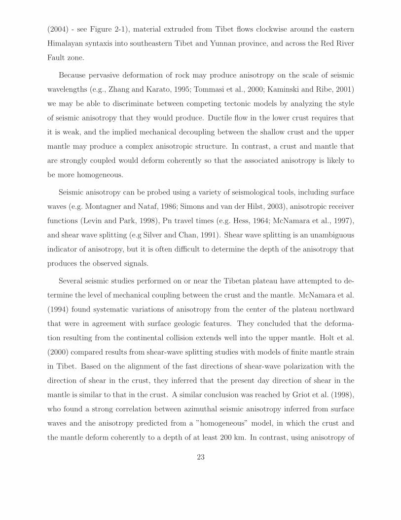
(2004) - see Figure 2-1), material extruded from Tibet flows clockwise around the eastern
Himalayan syntaxis into southeastern Tibet and Yunnan province, and across the Red River
Fault zone.
Because pervasive deformation of rock may produce anisotropy on the scale of seismic
wavelengths (e.g., Zhang and Karato, 1995; Tommasi et al., 2000; Kaminski and Ribe, 2001)
we may be able to discriminate between competing tectonic models by analyzing the style
of seismic anisotropy that they would produce. Ductile flow in the lower crust requires that
it is weak, and the implied mechanical decoupling between the shallow crust and the upper
mantle may produce a complex anisotropic structure. In contrast, a crust and mantle that
are strongly coupled would deform coherently so that the associated anisotropy is likely to
be more homogeneous.
Seismic anisotropy can be probed using a variety of seismological tools, including surface
waves (e.g. Montagner and Nataf, 1986; Simons and van der Hilst, 2003), anisotropic receiver
functions (Levin and Park, 1998), Pn travel times (e.g. Hess, 1964; McNamara et al., 1997),
and shear wave splitting (e.g Silver and Chan, 1991). Shear wave splitting is an unambiguous
indicator of anisotropy, but it is often difficult to determine the depth of the anisotropy that
produces the observed signals.
Several seismic studies performed on or near the Tibetan plateau have attempted to de-
termine the level of mechanical coupling between the crust and the mantle. McNamara et al.
(1994) found systematic variations of anisotropy from the center of the plateau northward
that were in agreement with surface geologic features. They concluded that the deforma-
tion resulting from the continental collision extends well into the upper mantle. Holt et al.
(2000) compared results from shear-wave splitting studies with models of finite mantle strain
in Tibet. Based on the alignment of the fast directions of shear-wave polarization with the
direction of shear in the crust, they inferred that the present day direction of shear in the
mantle is similar to that in the crust. A similar conclusion was reached by Griot et al. (1998),
who found a strong correlation between azimuthal seismic anisotropy inferred from surface
waves and the anisotropy predicted from a ”homogeneous” model, in which the crust and
the mantle deform coherently to a depth of at least 200 km. In contrast, using anisotropy of
23
the surface waves recorded at the INDEPTH-III array, Shapiro et al. (2004) found evidence
for thinning of and flow in the lower crust in Tibet. Ozacar and Zandt (2004) used receiver
functions to study crustal anisotropy, and also concluded that the middle crust in Tibet is
likely to be weak and deform ductily. Recently, Flesch et al. (2005) combined shear-wave
splitting measurements and geodynamical modeling to argue that the crust and the upper
mantle are coupled in central Tibet but decoupled in Yunnan. Finally, shear-wave splitting
measurements at an array north of the eastern Himalayan syntaxis (Figure 2-1, pink dots)
are consistent with crust-mantle coupling in much of eastern Tibet (Sol et al., 2005).
We report measurements of shear wave splitting at a temporary seismograph array de-
ployed in Sichuan and Yunnan provinces (Figure 2-1). Because our study region is located
in the proximity of the presumed transition between the deformation regime of Tibet and
that of Yunnan and south China (Flesch et al., 2005), our data may yield important insight
into the style of deformation in eastern Tibet. Indeed, the region’s oblique position to the
direction of convergence may enhance three-dimensional processes, which might be harder
to detect in the center of the plateau. Moreover, the unique structural features of eastern
Tibet, specifically the abundance of strike-slip faulting, provide us with a range of surface
observables that can be used to test proposed models.
Our analysis provides convincing evidence for anisotropy and shows that the source of
the inferred anisotropy is most likely located between 60 and 160 km depth (that is, in the
lower crust and the continental upper mantle), that the inferred orientation of strain in this
depth range differs from structural trends observed at the surface, in particular on the SE
flank of the plateau in Yunnan province, and that there is a distinct change in anisotropy
across the array from North-South orientations in the north to East-West in the south. The
latter may present evidence for a profound transition in lithosphere deformation regime,
which may have important implications for our understanding of the geotectonic evolution
of the Tibetan plateau.
24
2.3 Data and Methods
The data used here were recorded by a seismograph array operated by MIT and the Chengdu
Institute of Geology and Mineral Resources (CIGMR) between September 2003 and October
2004. The array consisted of 25 broadband seismometers (20 STS2 + 5 Guralp 3ESP)
from the IRIS-PASSCAL pool, deployed between latitudes 24◦N-32◦N and longitudes 99◦E-
101◦E (Figure 2-1). We also used data from the Global Seismograph Network (GSN) station
KMI, located in Kunming, Yunnan Province. In operation since 1992, and located within
our temporary array, KMI is an important source of data and an ideal reference for the
measurements made from our array.
With a deployment period of only 13 months, our array recorded SKS and SKKS data
from a relatively narrow range of back azimuths. Furthermore, most of the sources are at an
epicentral distance from which these core phases arrive within a time window shorter than
the wave-length, making the signal too complex for measuring splitting with the methods
used here. To increase the number of splitting measurements we also considered direct S
arrivals from events that are sufficiently deep that source-side anisotropy can reasonably be
ignored. There are several regions in the appropriate distance for such phases, including
the deep seismicity beneath the northwest Pacific island arcs, but none of them provided
high-quality splitting measurements.
Close to 3,000 SKS and SKKS phase arrivals from ∼350 teleseismic events (∆ = 85◦ −180◦) and a body-wave magnitude greater than 5.7 were recorded during the period of
deployment. From these, 300 records from a total of 41 events were selected through visual
inspection based on their signal-to-noise ratio and waveform clarity. Figure 2-2 depicts
locations of events used in the study. We used the cross-correlation method (e.g. Fukao,
1984; Levin et al., 1999) and the multichannel method (Chevrot, 2000) to calculate the
splitting parameters, that is, the azimuth of the fast polarization direction φ and the delay
time between the split phase arrivals, δt.
25
2.3.1 The Cross-Correlation method
A shear wave traveling through an anisotropic medium splits into orthogonally polarized fast
and slow components. The cross-correlation method attempts to maximize the similarity in
pulse shapes of these two components, which should ideally be identical, one delayed with
respect to the other. Following Levin et al. (1999), we estimate errors for individual records
assuming stochastic uncorrelated noise and applying a statistical F-test. With the individual
measurements thus obtained, we perform a grid search over possible values for φ and δt to
find the values that maximize the cross-correlation (Fukao, 1984). We search over a range
of φ from 0 to 180◦ and δt between 0.1 to 2.5 s to find a (φ, δt) that produces the smallest
root-mean-square misfit to the individual measurements. We estimate the error of the best
fitting parameters using the width of the minimal misfit region in the grid search. For
several stations the cross-correlation measurements vary widely (Figure 2-3), and estimating
an average fast direction was difficult. For the stations presented we estimate that the error
in the average φ is ±20◦ and the error in δt is ±0.2 s.
2.3.2 Multichannel method
The technique developed by Chevrot (2000) simultaneously utilizes phase arrivals from dif-
ferent back-azimuths. The amplitude of the transverse component for records with vari-
ous incoming polarizations is measured, and the azimuthal variation is compared with the
predicted variation for an assumed anisotropic medium. Provided that a broad range of
incoming polarizations is available, this method is convenient to use with phases of known
polarization, such as the core refracted SKS and SKKS. For a vertically incident shear wave
traveling through a single horizontal layer of transverse anisotropy, and under the condition
that δt is small compared to the dominant period of the signal, the radial (R) and transverse
(T) time series are given by the following expressions:
26
R(t) = w(t) (2.1)
T (t) = −1
2δt sin(2β) w(t),
where w(t) is the original waveform of the pulse, w(t) is the time derivative of w(t), and β is
the angle between the fast direction φ and the initial polarization of the pulse. The splitting
parameters can, therefore, be found by searching for the best fitting sin(2θ) curve to the
measured splitting vector. We calculate the error of individual splitting intensity measure-
ments using the correlation between the transverse component and the time derivative of
the radial component, as described in the appendix to Chevrot (2000). The error for the
splitting parameters estimated for each station may be large.
2.4 Results
2.4.1 Splitting parameters for a single-layer model
The average splitting parameters that best fit the data are listed in Table A1 (electronic
supplement) and illustrated in Figures 2-1 and 2-3. Figure 2-3a shows rose diagrams (angular
histograms) of the fast polarization directions (FPDs) calculated by the cross-correlation
method, as well as the estimate of the average fast direction under each of the stations.
For stations at which we were able to estimate splitting parameters with the multichannel
method, those measurements are also indicated. Figure 2-3b summarizes the best-fitting
FPDs for stations that are well constrained, along with major regional faults and surface
displacement field measured by GPS. As representative examples, we will describe below
the results for stations MC04 and MC08. At stations MC19 and MC20 not enough records
showed measurable splitting due to a low signal-to-noise ratio, and hence no results are
reported for them.
Station MC08 - located near the town of Jiulong, in the central part of the array
(Figure 2-3). The cross-correlation method yielded a wide range of fast directions and delay
27
times. Searching for the average value in this case is problematic (Figure 2-4 e,f). The
multichannel fit is better constrained, however, and hence this is the value illustrated in our
maps.
Figure 2-3 reveals a complicated pattern of fast directions. (We note that for stations
MC05, MC08, MC22, and MC25 we used the splitting parameters from the multi-channel
method.) First, for many of the stations the FPDs measured with the cross-correlation
method vary strongly with back-azimuth. Second, at eight stations both methods yield
good measurements, but the FPDs from them differ by 25◦ or more. Third, FPDs are quite
different from the main trends in the surface geology and in the GPS displacement field
(Figure 2-3b). Indeed, the correlation between the FPDs and the direction of faults is rather
poor (Figure 2-5a), although visual inspection suggests that it is better in the north than
in the south of the array. Furthermore, Figure 2-5b indicates that, in general, the FPDs
do not correlate with the directions of σSH as inferred from the World Stress Map project
(Reinecker et al., 2004).
Despite the scatter at individual stations, however, the measurements reveal a conspicu-
ous transition from mostly North-South oriented fast directions in the northern part of the
array (Figures 2-3 and 2-6a) to fast directions oriented mostly East-West in the southern
part of the array (Figures 2-3 and 2-6b). Interestingly, the fast polarization directions in the
South are – within error – parallel to the absolute plate motion (APM) in the region, which
is ∼ N100◦E according to NUVEL-1 (DeMets et al., 1994) (Figure 2-6).
2.4.2 Evidence for multiple layers of anisotropy?
It has been suggested, for instance by Levin et al. (2004) and Long and van der Hilst (2005),
that the kind of variability observed in some stations of our array (Figure 2-3) indicates
an anisotropic structure that is more complex than the single layer assumed initially. Also
the relationship between the FPD pattern and the main trends in the surface geology and
in the GPS displacement field (Figure 2-3) suggests significant complexity. Therefore, we
tested whether a model consisting of two horizontal anisotropic layers could explain the data
better. Since the two analysis methods described above assume a single anisotropic layer
28
with a horizontal fast axis, some modifications are necessary when a double-layer structure
is considered.
For a two-layer model, the splitting parameters measured with the cross-correlation
method are expected to depend strongly on the initial polarization of the waves (Silver
and Savage, 1994). For a vertical incidence the “apparent” splitting parameters vary with
back-azimuth with a π/2 periodicity (e.g. Rumpker and Silver, 1998). In this study we use
the algorithm due to Savage and Silver (1993) for predicting apparent splitting parameters
for a given double-layer model. We try to find a set of two pairs of splitting parameters
[(φ1, δt1), (φ2, δt2)], for the bottom and top layers respectively, that would give the best fit
to the measured apparent splitting parameters.
For the multichannel method the splitting intensity is the integration over depth of the
intensity caused by each of the layers through which the wave travels. Mathematically
this is equivalent to a summation of sinusoids, which is a sinusoid with a different phase and
amplitude. With this method it is, therefore, difficult to discriminate visually between a case
of multiple horizontal layers or a single layer. We performed a grid search over a range of
fast directions and delay times for a two layer model. The step size was 10◦ for direction and
0.1 s for delay time. The misfit was calculated using the root-mean-square of the difference
between the data and the model predictions, weighted by the individual errors.
Because of the limited azimuthal coverage, constraining a complex structure was difficult.
While the FPDs of the lower model layer could in most cases be constrained within ±10◦, the
upper layer was mostly unconstrained. Figure 2-4c,d and 2-4g,h display results for stations
MC04 and MC08. We find that, in general, a double-layer model does not significantly
improve the fit to the data. In some cases, however, using a double-layer model reduces the
disagreement between the results from analysis methods, which we regard as an improvement.
At station MC13, for instance, whereas the single-layer estimates of the two methods differ
by 42◦ (Figure 2-4i,j), the double-layer solution is within error for both of them (Figure
2-4k,l). We conclude that while a two layer model may be consistent with our observations,
the data considered thus far do not require it.
29
2.5 Discussion
One of the main results of our analysis is the clear north-to-south transition in the orienta-
tion of the FPDs (Figures 2-3 and 2-6). Exceptions to the trends, such as stations MC04,
MC05, MC13, and MC17, may be affected by local, near-station structure. Interestingly,
this transition appears to connect the trends inferred from studies in neighboring areas; Sol
et al. (2005) measure NW-SE trending FPDs to the northwest of our array (Figure 2-1, pink
dots), whereas Flesch et al. (2005) report East-West FPDs for Yunnan province, south of
our study region (Figure 2-1, orange dots).
2.5.1 Arguments for an upper mantle source of the splitting signal
An inherent limitation of using core-refracted waves such as SKS and SKKS to study
anisotropy is the path-integration of the signal, which makes it difficult to determine the
depth of anisotropy. However, the following observations give some insight about the depth
of the anisotropy. First, at many stations the inferred splitting time is > 0.6 s, which is
generally considered too large to be all of crustal origin (Barruol and Mainprice, 1993).
However, with a crustal thickness of 50-70 km this by itself is not a strong argument for
a sub-crustal origin. Second, the approximate width of the Fresnel zones of the recorded
phases help estimate the maximum and minimum depth of the anisotropy. For example,
the neighboring stations MC04 and MC08, separated by 117 km, show different splitting.
This suggests that the anisotropy has a fairly shallow source. Using a quarter-wavelength
approximation for the Fresnel zone width (Alsina and Snieder, 1995), we estimate that most
of the anisotropic signal probably originates above 160 km depth. On the other hand, the
comparison of the splitting of two events from opposing back-azimuths recorded at a single
station suggests a minimum depth of the anisotropy of 65 km.
Also the comparison with independent observations makes it unlikely that the anisotropy
inferred here has a near-surface origin. The regional strike-slip faults and the surface stress
field presumably reflect upper crustal processes. If the cause of anisotropy is the alignment
of crustal minerals by extensive shearing, or if the shear in the upper mantle is strongly
30
connected to that in the crust, we would expect the FPDs to align with strike-slip faults.
If, however, the source of anisotropy is the alignment of micro-cracks in the shallow crust,
the FPDs would align with the direction of the most compressive stress, σSH (e.g. Leary
et al., 1990; Peng and Ben-Zion, 2004). Figure 2-5 suggests that, in general, the FPDs in
the region under study correlate neither with the strikes of faults nor with the directions of
the most compressive stress, which suggests that the main source of anisotropy is unlikely
to be crustal.
2.5.2 Anisotropy in Yunnan province and near the Red River
Fault
The fast directions just north of the Red River fault zone are particularly intriguing, as
they suggest that the uppermost mantle is deforming in East-West direction, in contrast
with models that suggest that near-surface deformation is in North-South direction and
continuous across the fault (e.g. King et al., 1997). The situation in this part of our array
may, however, be more ambiguous than it may appear at first glance.
Strike-slip faults are the most prominent structural features in this part of our array.
In general, the strikes of these shear zones are approximately North-South, which is almost
perpendicular to the direction of the anisotropic fabric in the upper mantle as inferred
from shear wave splitting. It appears, however, that this area is actually undergoing rather
significant East-West extension (e.g. Wang and Burchfiel, 1997; Wang et al., 1998). The
driving force for this transtensional tectonics is not well known. It could be related to
distant subduction processes, including slab roll back, to the west (Andaman system) and
south-east (e.g., Philippines and Indonesia). Alternatively, it could reflect East-West strain
in the crust as it spreads out when it slides off the flanks of the plateau. The latter would be
consistent with the divergence in the directions of near-surface displacement inferred from
GPS measurements.
If the crust is indeed extending in that fashion, then the East-West trending fast direc-
tions we observe in the south would, in fact, align with surface processes, even if there is
substantial mechanical decoupling between the crust and the uppermost mantle. However,
31
the crust contribution to the splitting signal is probably minor (see previous section) and an
explanation must still be sought for the dramatic southward change in the deformation of
the uppermost mantle revealed by our splitting measurements.
2.5.3 Implications for lithosphere mechanics
The observations presented here give a first-order estimation of anisotropy in eastern Tibet
and have implications for our understanding of lithospheric deformation, including, perhaps,
the level of crust and mantle coupling in the region.
The splitting measurements suggest that the uppermost mantle is the most likely source
of the anisotropy measured here, and that its deformation geometry is different from that in
the crust. The anisotropy may be either a result of recent deformation, representing present-
day processes, or a fossilized fabric resulting of an older process. If we take the anisotropy to
represent the current deformation regime in the uppermost mantle beneath eastern Tibet,
then our observations and inferences are suggestive of mechanical decoupling of the upper
crust from the mantle, in particular in the south. We stress, however, that with the data
presented here we cannot rule out the contrary, and in the northern region within the plateau
such decoupling may not be required to explain the observations discussed here.
Irrespective of the level of crust-mantle decoupling, our results suggest a profound change
in deformation regime. Further studies are needed to establish the nature of transition in
more detail, but we postulate that it reflects a transition from collision controlled deformation
in the North and Northwest, including the Tibetan plateau itself, to deformation influenced
by other forces further to the South. The vertical resolution, limited when using teleseismic
shear-wave splitting, may be improved by using anisotropic receiver functions or through
the analysis of splitting in (P-S) conversions at the Moho or at intra-crustal interfaces.
Unfortunately, our array may not provide sufficient data for such detailed analysis. A more
promising approach toward constraining the radial variations of anisotropy would be the
tomographic inversion of relatively short-period surface wave dispersion (Yao et al., 2006).
32
2.6 Summary
We used shear-wave splitting to investigate seismic anisotropy and deformation in Eastern
Tibet. Even though there is significant scatter, the measurements based on the assumption
of a single layer of anisotropy reveal a conspicuous change in the fast direction pattern from
mostly North-South orientations in the north to mostly East-West in the south. Based on
the magnitude of delay times, the size of Fresnel zones, and the poor correlation between
directions of fast polarization on the one hand, and near-surface geology and geodetically
inferred surface displacement patterns, on the other hand, we argue that the anisotropy is
most likely located in the lower part of the thick crust and in uppermost mantle.
Distinguishing between different rheological models may be difficult based solely on the
shear-wave splitting measurements we present here. In the northern part of the array the data
may be consistent both with coherent deformation of the shallow crust and the uppermost
mantle and with mechanical decoupling between them. However, in Yunnan province and
the SE flank of the Tibetan plateau, the observations suggest differences in the deformation
patterns of the crust and mantle, and hence mechanical decoupling. The implied transition
between the northern and southern parts of our study region may reflect lateral variations
in lithosphere rheology, or a change in the tectonic regime, with the impact of the collision
weakening and that of far-field forces related to distant subduction processes strengthening
as we go southward. If corroborated by further study, this transition should be accounted
for in geodynamical models for the evolution of the Tibetan plateau.
Table 2.1: Preferred model results for all the stations. φ and δt are the fast direction andthe delay time estimated, respectively.
2.8 Figures
34
90°E 95°E 100°E 105°E
25°N 25°N
30°N 30°N
35°N 35°N
Red R
iver F
ault
Sichuan Basin
TibetanPlateau
APM
Yunnan
In
do
-Bu
rma
Su
bd
uctio
n syste
m
MIT array - blue symbols
Figure 2-1: Location of the seismic stations used in this study (blue dots) and the fastpolarization direction estimated for them. The background shows the topography of EastAsia and the regional faults (dark green - left-lateral strike-slip faults, light green - right-lateral strike slip faults, pink - thrust faults). RRF = Red River Fault. APM = the localabsolute plate motion direction, NUVEL-1 (DeMets et al., 1994). Previous shear wavessplitting results are also shown: Green dots - Huang et al. (2000); Red dots - McNamaraet al. (1994); Orange dots - Flesch et al. (2005). Pink dots depict the location of the seismicstations used by Sol et al. (2005). Red arrows denote geodetically measured surface velocitiesrelative to the South China block (after Chen et al., 2000; Zhang et al., 2004).
35
Figure 2-2: Epicenters of events used in the study (red dots). We use a total of 41 events ofmagnitude 5.7 and above.
36
KMIMC25
MC24
MC23
MC22
MC21
MC20 MC19
MC18
MC17
MC16
MC15
MC14MC13
MC12
MC11
MC10MC09MC08MC07MC06
MC05MC04 MC03
MC02
MC01
25°N
Red
River
Tibetan
Plateau
25°N
Sichuan
Basin
A B
30°N
100°E 105°E
30°N
100°E 105°E
25°N
Figure 2-3: Splitting measurements in eastern Tibet (assuming a single-layer). (a) Foreach station, we show an angular histogram of the measurements obtained using the cross-correlation method (blue). Cyan lines show the angular average. Where applicable, red linesin the histograms give the fast direction obtained using the multichannel method. RRF -Red River Fault; (b)Average fast directions for well-constrained stations (black lines). Redarrows denote surface displacement vectors from Chen et al. (2000) and Zhang et al. (2004).Green lines show the major regional strike-slip faults.
37
MC04a b c d
0 100 200 300−1.5
−1
−0.5
0
0.5
1
1.5
Back Azimuth (°)
Spl
ittin
g In
tesn
ity
φ = 86°δt =1.1 δt=1.06s
φ = 60°
φMC
=86°
0 100 200 300−1.5
−1
−0.5
0
0.5
1
1.5
Back Azimuth (°)
Spl
ittin
g In
tens
ity
φ1=90,δt
1=2.4
φ2=20,δt
2=0.7
0 50 100 1500
50
100
150
200
Back Azimuth (°)
φ (°
)
φ1=90°,δt
1=2.4
φ2=20°,δt
2=0.7
MC08e f g h
0 100 200 300−1.5
−1
−0.5
0
0.5
1
1.5
Back Azimuth (°)
Spl
ittin
g In
tesn
ity
φ=0°δt=1
φMC
=0°
δt=1.2sφ=110°
0 100 200 300−1.5
−1
−0.5
0
0.5
1
1.5
Back Azimuth (°)S
plitt
ing
Inte
nsity
φ1=0°,δt
1=1.6
φ2=120°,δt
2=0.8
0 50 100 150
50
100
150
200
Back Azimuth (°)
φ (°
)
φ1=0°,δt
1=1.6
φ2=120°,δt
2=0.8
MC13i j k l
0 100 200 300−1.5
−1
−0.5
0
0.5
1
1.5
Spl
ittin
g In
tesn
ity
Back Azimuth (°)
δt=0.63φ=38°
φ=38°
φ=70°δt=0.43
0 100 200 300−1.5
−1
−0.5
0
0.5
1
1.5
Back Azimuth (°)
Spl
ittin
g In
tens
ity
φ1=30°,δt
1=1.2
φ2=100°,δt
2=0.8
0 50 100 1500
50
100
150
200
Back Azimuth (°)φ
(°)
φ1=30°,δt
1=1.2
φ2=100°,δt
2=0.8
Figure 2-4: Results for station MC04, MC08, and MC13. Shown are 2σ error bars. Fromthe left:a,e,i - Splitting intensity measurements from the multichannel method (blue), with the redcurve the fit assuming a single layer of anisotropy; b,f,j - rose diagram of FPD measurementsfrom the cross-correlation method (blue), with mean direction indicated in cyan; c,g,k -Splitting intensity measurements, with a fit based on a double layer of anisotropy; φ1, δt1 aresplitting parameters for the bottom model layer, sampled first, and φ2, δt2 are the splittingparameters for the model top layer, sampled second; d,h,l - Measured fast directions vs.back-azimuth (blue) and the predicted fast direction assuming a double layer model (red);
38
0 20 40 60 800
0.5
1
1.5
2
2.5
3
3.5
4
4.5
5
Angle Difference (°)
num
ber
φ−Fault AzimuthA
0 20 40 60 800
0.5
1
1.5
2
2.5
3
3.5
4
4.5
5
Angle Difference (°)
num
ber
φ − σsh
B
Figure 2-5: Testing the correlation of fast polarization directions with surface features: His-togram of angular difference between measured FPDs and nearest fault strike (a) and localmost compressive stress direction σSH as estimated from the world stress map. (b). We notethat FPDs of stations MC02, MC07, MC10 and MC13 are not compared to faults becausethey are too far from mapped strike-slip faults. No fast directions were calculated for MC19and MC20, due to insufficient data.
Fast directions in the NORTHMC01−MC18
mean
APM
Fast directions in the SOUTHMC21−MC25, KMI
mean
APM
Figure 2-6: Rose diagram for the average FPDs of the stations in the northern and centralparts of the array (left) and in the south (right). Average FPDs for stations MC01 throughMC18 are included in the northern and central region. Average FPDs for stations MC21through MC25 and KMI are included in the southern region. The mean direction and theNUVEL-1 absolute plate motion (APM) direction are indicated. These summary diagramsdemonstrate that there is a transition from a NNW-SSE trend in the north and center to anE-W trend in the south.
39
40
Chapter 3
Rayleigh-Taylor instabilities with
anisotropic lithospheric viscosity
3.1 Abstract
Rocks often develop fabric when subject to deformation, and this fabric causes anisotropy
of physical properties such as viscosity and seismic velocities. We employ two-dimensional
analytical solutions and numerical flow models to investigate the effect of anisotropic vis-
cosity on the development of Rayleigh-Taylor instabilities, a process strongly connected to
lithospheric instabilities. Our results demonstrate a dramatic effect of anisotropic viscosity
on the development of instabilities - their timing, location, and, most notably, their wave-
length are strongly affected by the initial fabric. Specifically, we find a significant increase in
the wavelength of instability in the presence of anisotropic viscosity which favors horizontal
shear. We also find that an interplay between regions with different initial fabric gives rise
to striking irregularities in the downwellings. Our study shows that for investigations of
lithospheric instabilities, and likely of other mantle processes, the approximation of isotropic
viscosity may not be adequate, and that anisotropic viscosity should be included.
0Published as: Lev, E. and B.H. Hager, Rayleigh-Taylor Instabilities with anisotropy lithospheric viscosity,Geophys. J. Int. 173 (2008), p. 806-814.
41
3.2 Introduction
The response of anisotropic materials to stress depends on the orientation of the stress relative
to the orientation of the anisotropy. Anisotropy of seismic wave speed in rocks has been
studied vigorously in the last decades, both in experimental (e.g. Zhang and Karato, 1995)
and theoretical work (e.g. Kaminski and Ribe, 2001). It has been shown that the deformation
of rocks and minerals leads to development of crystallographic preferred orientation (CPO),
which leads to seismic anisotropy (Karato et al., 1998). In addition, rotation of grains and
inclusions, alignment of micro-cracks or melt lenses, and layering of different phases all lead
to the development of shape preferred orientation (SPO), an important source for seismic
anisotropy (e.g. Crampin, 1978; Holtzman et al., 2003; Maupin et al., 2005).
The anisotropic viscosity (AV) of earth materials has received less attention, but its
effects are dramatic. Using laboratory experiments, Durham and Goetze (1977) showed
that the strain rate of creeping olivine with preexisting fabric depends on the orientation
of the sample and can vary by up to a factor of 50. This is because the orientation of the
sample relative to the applied stress determines which slip systems are activated. In the
experiments of Bai and Kohlstedt (1992) on high-temperature creep of olivine and those
of Wendt et al. (1998) on peridotites, the measured strain rate depended strongly on the
relative orientation of the applied stress to the sample crystallographic axis. Honda (1986)
calculated the long-wavelength constitutive relations for a transversely isotropic material,
and concluded that these can be characterized by two viscosities - a normal viscosity (ηN),
associated with principal stresses normal to the easy-shear planes, and a shear viscosity
(ηS), associated with shearing parallel to the easy-shear planes. More theoretical work (e.g.
Weijermars, 1992; Mandal et al., 2000; Treagus, 2003) was done to assess the AV of composite
materials, depending on the geometry and the relative strength of each component. These
studies imply that regions of the earth that are not likely to become anisotropic by means of
dislocation creep and LPO development may exhibit AV due to the deformation of composite
materials, such as most natural rocks, and two-phase materials, such as partially-molten
rocks. Recently, Pouilloux et al. (2007) discussed the anisotropic rheology of cubic materials
and the consequences for geologic materials.
42
A few geodynamical studies have examined the effect of AV on mantle flow. Richter
and Daly (1978) and Saito and Abe (1984) used analytical solution methods to investigate
the development of Rayleigh-Benard instabilities in a viscously anisotropic medium with
specified easy-shear geometry, and found a connection between the anisotropy of the fluid
and the length-scales of the convection cells. In a very instructive study a few years later,
Christensen (1987) showed that the inclusion of AV affects two important mantle flows
- postglacial rebound and thermal convection. For example, Christensen (1987) pointed
out a spatial offset between mass anomalies and the resulting geoid signal in the presence
of AV, which may help to reconcile the argued mismatch between observed uplift history
near ice sheet margins and models of strong viscosity stratification in the mantle. AV also
leads to channeling of flow into low viscosity region such as hot rising plumes. Nonetheless,
Christensen concluded that the actual effect of AV in the earth’s mantle would be much
smaller, as the fabric required for creating AV would be obliterated by the highly time-
dependent flow. However, the abundant evidence for seismic anisotropy in the earth and its
strong correlation with tectonic processes and features suggest that large parts of the mantle
maintain fabric for long times. Pre-existing mechanical anisotropy in the lithosphere was
shown to have an effect in various tectonic settings such as oceanic shear zones (Michibayashi
and Mainprice, 2004) and continental break-up parallel to ancient orogens (Vauchez et al.,
1998).
Recently, Moresi, Muhlhaus and co-workers (e.g. Moresi et al., 2002, 2003) presented an
efficient algorithm for including an AV that evolves with the flow in geodynamical models.
They demonstrated the new algorithm in a series of papers, looking at various geological
problems, including folding of a layered medium and thermal convection. We employ this
technique here to investigate lithospheric instabilities in the presence of AV.
The lithosphere is often identified as the cold upper thermal boundary layer of Earth’s
convecting mantle. The colder temperature of the lithosphere makes it more dense than
the asthenosphere underneath, and leads to an unstable density layering (Houseman et al.,
1981). This density instability may be further enhanced by thickening of the lithosphere
due to convergence (Molnar et al., 1998) or emplacement of dense material (eclogite) at
43
the base of the lithosphere (Elkins-Tanton and Hager, 2000). Lithospheric instabilities and
removal of the lower lithosphere have been invoked to explain observations in the New
England Appalachians (Robinson, 1993), the Canadian Appalachians (Murphy et al., 1999),
Europe (Wenzel et al., 1997), Argentina (Kay et al., 1994), the North China craton (Fan
et al., 2000; Wu et al., 2005) and Tibet (England and Houseman, 1989). Regions of high
seismic velocity underneath southern California (Humphreys and Clayton, 1990; Kohler,
1999; Yang and Forsyth, 2006) are also interpreted as cold material sinking from the bottom
of the lithosphere, probably as part of three-dimensional small-scale convection in the region
(Humphreys and Hager, 1990) or Rayleigh-Taylor instabilities (Billen and Houseman, 2004).
Upwelling of hot asthenospheric material following removal of the lower lithosphere has been
suggested to explain, for instance, the massive flood basalts in Siberia (Elkins-Tanton and
Hager, 2000).
The removal of the bottom of the lithosphere due to a density instability can be ap-
proximated as a Rayleigh-Taylor instability (Conrad and Molnar, 1997). Previous studies of
Rayleigh-Taylor instabilities addressed the effect of the density structure, the wavelength of
the density perturbation between the layers, and the rheology of the layers, on the timing
and location of instability onset (e.g. Whitehead, 1986; Conrad and Molnar, 1999; House-
man and Molnar, 1997; Billen and Houseman, 2004). Here we demonstrate the significance
of pre-existing and evolving fabric.
3.3 Anisotropic viscosity and the wavelength of insta-
bilities
We begin our investigation with a simple conceptual setup: a dense anisotropic layer laying
over a more buoyant isotropic half-space. All of the models in this study are two-dimensional.
The interface between the two layers is perturbed by a small initial displacement w(x) =
w0 cos (kx), where x is the horizontal direction, and k is the wave number of the interface
perturbation. Our goal in this section is to examine the dependence of the growth rate of
instabilities on the wave number of the perturbation, the initial orientation - horizontal or
44
dipping - of the easy-shear planes, and the ratio between the shear and normal viscosities.
We use both an analytical solution and numerical experiments for this purpose.
3.3.1 Governing equations
We treat the mantle as an incompressible fluid, an approximation valid for slow viscous
deformation in the upper mantle (e.g. Schubert et al., 2001). The main equation to be
solved is conservation of momentum:
∂σij
∂xj
− ∂p
∂xi
+ fi = 0 (3.1)
where σij is the deviatoric stress tensor, p is the pressure, fi is the force acting in the i-th
direction, and inertia is neglected. For our case, fz = ρgz, where z is the vertical coordinate.
The flow also has to fulfill the continuity requirement for an incompressible material:
∂vi
∂xi
= 0 (3.2)
where v is the velocity.
A central equation for any flow model is the constitutive law, relating stress and strain
in the system. The constitutive law we use in this study reflects the anisotropic rheology of
the materials. The simplest form of anisotropy is transverse isotropy (TI), as for a deck of
cards. As shown by Honda (1986), a TI material can be characterized by two viscosities - a
normal viscosity, ηN , and a shear viscosity, ηS. This form of anisotropy can describe both a
layered medium, consisting of layers of different strength, or the crystallographic preferred
orientation of anisotropic minerals with a dominant easy glide plane. The normal viscosity
governs deformation when the two principle stresses are oriented normal and parallel to the
glide plane, while the shear viscosity governs deformation when the principle stresses are
oriented at 45◦ to the glide plane. The exact expressions we use for our analysis are given
in equations (3.4) and (A1).
We note that in this formulation, materials with horizontal and vertical easy-shear direc-
tions are mathematically equivalent. This is similar to a stack of books on a shelf - it is easy
45
to shear the stack horizontally both when the books stand up (vertical easy-shear planes)
and when they lay on top each other (horizontal easy-shear planes).We thus examine two
end-member setups - in one the anisotropic dense layer initially has a horizontal easy-shear
direction, and in the other the easy shear direction initially dips at 45◦.
3.3.2 Analytical solution
In this analysis we use the propagator matrix technique (e.g. Hager and O’Connell, 1981)
to calculate the growth rate of the instabilities as a function of the wavelength of a small
perturbation in the interface between the two materials. The mean depth of the interface
is at z = 0. The boundary conditions for our problem are no-slip at the top boundary
(z = 1), which we take to be the base of the rigid part of the lithosphere, and vanishing of
the velocities and stresses as z → −∞. By calculating the vertical velocity v(z = 0) we are
able to track the change in position of the boundary. The derivation is outlined in Appendix
A, and an important outcome of it is that
v(z = 0) ≡ ∂w
∂t∝ w (3.3)
Because the velocity of the interface is proportional to the amplitude of the boundary topog-
raphy (eqn. 3.3), the change in the interface depth follows an exponential growth rule:
w(z, t) = etτ . τ , the growth rate, is a function of the wave number k of the perturbation w,
and of the two viscosities ηN and ηS.
The results we present in section 3.3.4, as well as Appendix A, give insight into the
relationship between the growth rate and a range of viscosities and wave numbers. We note
here that this analysis is valid only for small interface perturbations, so we can assume that
the orientation of the AV does not evolve.
3.3.3 Numerical experiments
To follow the instability to finite amplitude requires a numerical approach. We solve the flow
equations using a finite element formulation on an Eulerian mesh embedded with Lagrangian
46
integration-points (“particles”), as described by Moresi et al. (2003). In this method, par-
ticles carry the material properties, and foremost their deformation history and the derived
AV. Variables such as velocity and pressure are calculated at the location of the mesh nodes,
which are fixed in space. We use the software package Underworld (Moresi et al., 2007) to
solve the flow equations.
Including anisotropy in the flow equations
To include AV in our numerical experiments, we use the particle-in-cell formulation (Moresi
et al., 2003). By this method, the anisotropy is represented by a set of directors advected
through the model, analogous to particles (Muhlhaus et al., 2002b). The directors are
vector-particles pointing normal to the easy-glide plane or layer, thus defining the directions
associated with ηN and ηs. In each time step of the calculation, the directors are advected
and rotated by the flow, and in return determine the viscosity structure for the next time
step (Muhlhaus et al., 2004).
The AV enters the equation of momentum through a ‘correction’ term added to the
isotropic part of the constitutive equation relating stress and strain rate (Muhlhaus et al.,
2002b):
σij = −pδij + 2ηN ǫij − 2(ηN − ηS)Λijklǫkl (3.4)
where ηN , ηS are the normal and shear viscosities, respectively, σ is the deviatoric stress
tensor, and ǫ is the strain rate tensor. Λ reflects the orientation of the directors in space,
diamonds) and isotropic (black line, circles). The results agree with the predictions from the
analytical solution presented above - the fastest growth rate for the horizontal fabric is at a
longer wavelength than that for the dipping fabric or for an isotropic layer, and the curve
is indeed flatter at longer wavelengths. The minimum growth rate for a dipping fabric is
at almost the same wavelength as that for an isotropic material, again in agreement with
the analytical predictions. Figure 3-3 shows the material distribution in the different model
configurations after the fastest drips have sunk half of the box depth, as well as the approxi-
mate location of the initial perturbed interface (yellow curve). These snapshots demonstrate
clearly that the wavelength of the instabilities developing in the initially horizontal models
is greater than of those developing in the initially-dipping models. This emphasizes the
advantage gained by using numerical experiments - the analytical solution gives insight into
the behavior of instabilities at small amplitudes, while the numerical experiments are essen-
tial for predicting the behavior as the flow progresses and instabilities of finite-amplitude
develop.
49
3.4 Laterally-varying anisotropy
Intrigued by the dramatic results for a simple model of a homogeneous anisotropic dense
layer described above, we proceed and use numerical experiments to examine the effect of
including lateral variations in the initial anisotropic fabric of the dense layer.
3.4.1 Model setup
Figure 3-4 depicts the model geometry and initial and boundary conditions. The model
domain is again a rectangular box with an aspect ratio of 1:6.4. The location and amplitude
of the interface between the layers is the same as in section 3.3. Following the findings of
section 3.3, we perturb the interface with a wavelength long enough to allow deformation at
a wide range of wavelengths to develop freely. The dense layer now contains two anisotropic
regions in the center, each 1.6 wide, and two isotropic regions of the same high density
near the edges. The anisotropic regions differ only by their initial fabric orientation - one
(shown in red) initially has a horizontal easy shear direction, and the other has an easy shear
direction initially dipping at 45◦ (shown in yellow). The viscosity of the buoyant layer is
equal to the normal viscosity of the anisotropic layer. The shear viscosity of the anisotropic
material is a factor of 10 less than its normal viscosity. We shift the anisotropic regions
laterally in different models in order to change the phase between the viscosity structure
and the density interface perturbation. We then examine the development of drips for each
configuration.
3.4.2 Results - a heterogeneous upper layer
In figure 3-5 we show the instabilities that develop in our models. The different panels depict
models with different configurations of the initial fabric domains, shown in red and yellow, as
well as the results for an isotropic model for comparison (Fig. 3-5a). We also show the trace
of the original density interface between the dense lithosphere and the underlying mantle
(black horizontal curve) and the location of the deepest points of the initial perturbation of
the density interface (dashed vertical lines).
50
Several first-order observations can be made in figure 3-5. First, there is a striking dif-
ference between the instabilities that develop in the two anisotropic domains. Most notably,
the wavelengths of the downwellings that develop in the domain with easy horizontal shear
are much longer than the wavelengths in the dipping-fabric domains or in the isotropic model
(Fig. 3-5a). In addition, the domain which starts with easy horizontal shear (red) devel-
ops instabilities faster than the domain which starts with easy shear direction dipping at
45◦ (yellow). Next, for several situations, the fastest-growing downwelling does not coincide
with the locations of maximum thickness of the dense layer, but is offset horizontally by up
to 0.5 of the box depth (Fig. 3-5b,g). Finally, almost all of the fastest-growing instabilities
occur near the edges of the domain of horizontal easy shear (excluding the case where the
thickest part of the dense layer was exactly in the center of the domain of initial horizontal
anisotorpy), but the instabilities that develop in the dipping easy shear domain develop in its
interior. Evidently, the initial fabric and its lateral variations influence the flow significantly.
3.5 Discussion
Our models are set up in a non-dimensional manner, for generality. It is interesting, though,
to re-scale the results to lithospheric dimensions. The dense layer (top 15% of the box)
corresponds to the viscously-mobile part of the lithosphere, which is approximately its lowest
40 km. The viscosity of the lithosphere is temperature-dependent, and is believed to decrease
exponentially with depth, with a reasonable decay length of about 10 km (Molnar et al.,
1998). If we take the viscosity at the base of the lithosphere to be 1019 Pa s (Hager, 1991),
then the average viscosity for a 40 km thick layer, calculated as < η >= exp( log η1+log η2
2),
is 7.4 · 1019 Pa s. Using the thickness of the lower lithosphere as the characteristic length
scale, we can estimate the spacing between the isotropic instabilities as 130 km, and the
wavelength of the longest anisotropic instabilities is close to 400 km. The lateral offset
between the downwellings and the locations of maximum lithospheric thickness scales to a
maximum of approximately 150 km. We re-scale velocities based on the the viscosity and
density contrast, using the “Stokes Velocity” (VStokes = ∆ρ∗g∗h2
η, where η is the effective
51
viscosity of the dense layer, ∆ρ is the density contrast and h is the dense layer thickness).
We estimate the difference between the density of the lower lithosphere and the density of the
underlying asthenosphere as 40 kg/m3 (Molnar et al., 1998). After substituting the above
values we can now calculate the scaling of time. We estimate that the time it takes for the
drips to sink to a depth of 160 km (the stage shown in Fig. 3-5) is approximately 12 Myrs.
This duration is within the range of times estimated by Houseman and Molnar (1997) for
removal of the base of an unstable thickened lithosphere. This time and distance of sinking
imply an average sinking velocity of 14 mm/yr.
The models we present here are a preliminary attempt at this problem, and thus have
some shortcomings when compared with the lithosphere. First, the fabric development rule
we use is a simple rotational evolution law, and does not take into account factors such as
temperature, strain rate, and recrystallization, all known to affect the development of CPO
in rocks. Second, the rheology we use is a Newtonian creep law, while in fact anisotropy
due to CPO requires deformation in the dislocation creep regime, which is a power-law
creep process. Additionally, all our experiments are carried out in two dimensions. There
may be interesting consequences when these effects are studied in a three-dimensional setup,
especially given the three-dimensional nature of some observed mantle instabilities (e.g. Yang
and Forsyth, 2006). A three-dimensional model would also be able to include orthorhombic
symmetry and would not be constrained to the use of transverse isotropy. Hopefully future
work would be able to assess the significance of these factors and their implications.
Both our analytical solution and the numerical flow models predict that the wavelength of
Rayleigh-Taylor instabilities would be longer for an anisotropic material, most significantly
for a fabric favoring horizontal flow. Some intuitive understanding of this can be gained if we
imagine a horizontally layered medium - it is much easier for such a medium to flow sideways
by simple shear, and not to develop vertical drips. Drips will eventually develop in locations
where the horizontal flow encounters resistance - for instance in the form of a domain with a
different fabric. This is likely the reason that the largest downwellings developed in the edges
of the domains with initial horizontal easy shear direction (red domains in Fig. 3-5). If, on
the other hand, the initial fabric is at an angle to the main acting force, it will be easier for
52
the instabilities to thicken by pure shear and ‘break’ the layering structure, and hence will be
more likely to follow a wavelength closer to the isotropic one. This result is in agreement with
the experiments of Richter and Daly (1978), who found that anisotropy leads, in general,
to longer wavelengths of instabilities. Saito and Abe (1984) performed a marginal stability
analysis for a related model setup (bottom-heated Rayleigh-Benard convection with stress
free boundaries and horizontal layering) and, similarly to our results, found that the stability
curves flatten out and that the minimum shifts to a longer wavelength with lower viscosity
ratio.
We emphasize at this point that numerical techniques such as the one we use here have
several important advantages. Analytical solutions, while elegant, give insight into the be-
havior of instabilities only at small amplitudes, and thus numerical experiments are essential
for predicting the flow as it progresses and instabilities of finite-amplitude develop. Addi-
tionally, the numerical technique we use is capable of modeling flows in which the fabric
is evolving and the orientation of the anisotropy is not fixed in space, as opposed to the
situation in our, as well as earlier (e.g. Richter and Daly, 1978; Honda, 1986), analytical
solutions. It is also straightforward to include lateral variations of the anisotropy, a scenario
highly relevant to tectonic processes in natural environments.
The strong effect of pre-existing fabric on the development of Rayleigh-Taylor instabilities
may have important implications for the stability of the lithosphere. In our models, the
fastest growing downwelling sometimes develops away from the initially deepest region of
the density interface, due to the interaction between domains with different fabric orientation.
This change in geometry may provide a simple explanation for the offset of the mantle drip
beneath the Sierras (e.g. Saleeby and Forster, 2004). Our findings of the effect of AV on the
wavelength of instabilities should also be considered in the context of other locations, for
example Tibet. Conrad and Molnar (1997) argued that the wavelength of Rayleigh-Taylor
instabilities predicted to arise from the collision between India and Eurasia is much shorter
than the wavelength of the Tibetan plateau, and hence such instabilities are unlikely to be
the cause of the rapid uplift of the plateau at 5-10 Myrs ago. If, however, the existing fabric
in the collision zone was such that it leads to longer wavelengths, this possibility may need
53
to be reconsidered.
The points of contact between regions with different existing fabric appear to have unique
significance. This hints that when tectonic units which have gone through a different evo-
lution and developed different fabric are juxtaposed, this contact point may be particularly
unstable. An example of such a situation may be the placing of a spreading center, which
is characterized by horizontal easy-shear planes, next to a region that is more horizontally-
resistant. When this combination is put under compression, the horizontal easy shear planes
will be unstable at the contact point, which may lead to initiation of downwelling and perhaps
even subduction. Subduction initiation at extinct spreading centers is likely the explanation
for the subduction zone at the Macquirie region south of New-Zealand (Lebrun et al., 2003)
and near the Oman ophiolite (Michibayashi and Mainprice, 2004). Our results clearly show
that additional knowledge of the anisotropic fabric of the lithosphere, and, specifically, the
orientation of dipping fabrics, can shed light on different tectonic problems, and highlights
the importance of overcoming the difficulties in making such measurements (e.g. Chevrot
and van der Hilst, 2003).
3.6 Summary
We show the dramatic effect of anisotropic viscosity on the development of Rayleigh-Taylor
instabilities. The wavelength, timing and shape of the instabilities that develop in our
models are strongly affected by the initial fabric prescribed. The most notable effect of
anisotropic viscosity on Rayleigh-Taylor instabilities, demonstrated here both analytically
and numerically, is the shift to longer wavelengths when the initial fabric of the dense material
favors horizontal flow (horizontal or vertical fabric). The interplay between regions with
different orientations of initial fabric gives rise to a variety of features, such as an offset of the
main downwellings away from the deepest point of the perturbed interface, and demonstrates
the importance of considering the deformation history of all the units participating in a
tectonic setting. Our results show that for the study of lithospheric instabilities, and likely
of other mantle processes, the common isotropic approximation may not be accurate, and
54
hence anisotropic viscosity should be included.
Acknowledgements. We are grateful for helpful discussions with Linda Elkins-Tanton,
Ming Fang, Greg Hirth, Eduard Kaminski, Laurent Pouilloux, and Andrea Tommasi. A
thoughtful review by Gregory Houseman helped greatly to improve this manuscript. The
research presented here was supported by NSF under grants EAR-0337697 and EAR-0409564
55
3.7 Appendix A: Derivation of analytical solution
We begin by defining the following anisotropic constitutive relations, which describe a trans-
versely isotropic (TI) material in the two special cases considered here of 1) easy-shear on
horizontal/vertical planes and 2) easy-shear on planes dipping at 45◦:
σxx = 2ηpsǫxx (A1a)
σzz = 2ηpsǫzz (A1b)
σxz = ηssǫxz (A1c)
where ηps is a viscosity corresponding to pure shear stresses, and ηss corresponding to simple-
shear. For a material with a horizontal easy-shear direction (horizontal layering, for instance)
ηss is equivalent to ηS defined in section 3.3.1, ηps ≡ ηN , and ηss < ηps. For an anisotropic
material with a dipping easy-shear direction, ηS ≡ ηps < ηss ≡ ηN . For an isotropic material,
ηps = ηss. This constitutive relation can be derived from a matrix form similar to that in
equation 3.4: σij = 2ηNǫij − 2(ηN − ηS)Λijklǫkl where Λ is an alignment tensor reflecting
the orientation of the symmetry axis. Then, the transformation from a horizontal symmetry
anisotropy to a dipping symmetry can be achieved by a rotation of the 4th-order tensor Λ.
In our analytical solution, we employ the propagator matrix technique (e.g. Hager and
O’Connell, 1981) to calculate the growth rate of Rayleigh-Taylor instabilities as a function
of the wavelength of the density perturbation between the two materials. We set z = 0 at
the interface between the layers, z = 1 at the top of the dense layer, and the initial location
of the density interface as w = w0 cos(kx). For the horizontal and 45◦-dipping orientations
we consider here, this definition of the interface perturbation leads to vx, σzz ∝ cos(kx), and
vz, σxz ∝ sin(kx), where k is the wave number. For other orientations there may be a phase
shift with depth (Christensen, 1987). Thanks to the orthogonality of the trigonometric basis
functions, we can write a simplified set of equations for each wave number. We define a
vector u = [v, u, σzz, σxz], where v is the vertical velocity, u is the horizontal velocity, σzz is
the normal stress in the z direction, σxz is the shear stress, and x and z are the horizontal
56
and vertical coordinates. After some manipulation, this definition of u enables us to express
the equations of flow in each layer for every k as
Du = Au + b (A2)
where D = ∂∂z
, and b is a forcing term. The matrix A is where the anisotropic viscosity is
manifested.
The definition of the anisotropic constitutive relation above leads to a matrix A of the
form:
A =
0 −k 0 0
k 0 0 η−1ss
0 0 0 −k
0 4ηpsk2 k 0
(A3)
When ηps = ηss (isotropic material), the expression in (A3) is equal to the matrix A given by
Hager and O’Connell (1981). Otherwise, it reflects the anisotropic viscosity of the material
by including the two different viscosities.
The solution to equation (A2) is of the form
u(z) = eA(z−z0)u(z0) +
∫ z
z0
eA(z−ξ)b(ξ)dξ (A4)
We define the propagator matrix P(z, z0) = eA(z−z0), so that the velocities and stresses can
be expressed as
u(z) = P (z, z0)u(z0) +
n∑
i=1
P (z, ξi)b(ξi)∆ξi (A5)
where ξi is the depth at the center of a the i-th layer and ∆ξi is the layer thickness. The
propagator matrix for an anisotropic material will naturally be different than the propagator
matrix for an isotropic material, given the difference in the corresponding A matrices. The
boundary conditions for our problem are no-slip at the top boundary (z = 1), which we take
to be the base of the rigid part of the lithosphere, and vanishing of the velocities and stresses
57
as z → −∞. We can express the boundary conditions using the vector u defined earlier:
u(z = 1) = [0, 0, σtzz, σt
xz], u(z = −∞) = [0, 0, 0, 0] (A6)
In order to fulfill the boundary condition as z → −∞, u just below the interface has to be
of the form u(z = 0−) = [C1/2k, C2/2k, C1, C2], where C1, C2 are the σzz and σxz at the
interface. We add a normalized forcing term which here represents the gravitational forcing
in the z direction. Thus u across the interface, at the bottom of the dense layer, becomes
u(z = 0+) = [C1/2k, C2/2k, C1 + 1, C2]. We propagate this u(z = 0+) upwards to the top
interface using the anisotropic propagator matrix Pani: u(z = 1) = Paniu(z = 0+). From
the no-slip boundary condition at the top, the first two components of the resulting vector
are equal to zero. We now have two equations and two unknowns - C1 and C2. We solve for
these two unknowns and use the result to calculate the vertical velocity at the interface.
The change in the interface location with time is equal to the vertical velocity at the
interface - v(z = 0), where v is the vertical velocity. A result of the derivation described
above is that the vertical velocity at the interface is proportional to the perturbation of the
interface, that is:
v(z = 0) ≡ ∂w
∂t∝ w (A7)
Therefore the change in the interface depth follows an exponential growth rule: w(z, t) = etτ ,
which gives the dependence of the growth rate τ on the model parameters:
τ =1
K(ηps, ηss, k)(A8)
K is a complicated function of the viscosities and the wave number, of the form
∆ρg×[a sum of exponents of powers of ηN , ηs, and k]. The exact expression is too long to give
here explicitly, but can be obtained using the Matlab code in the electronic supplement. The
resulting relationship between 1/K (τ) for a range of wave numbers and a set of viscosity
ratios is demonstrated in figure 3-1; Figure S1 (Electronic Supplement) shows a similar
calculation for a range of viscosity ratios and k = 0.1.
58
A careful inspection of the anisotropic matrix Aani and the anisotropic propagator matrix
Pani reveals a very interesting phenomenon - an oscillatory behavior with depth for certain
viscosity ratios. Let us define δ, the viscosity ratio, as δ = ηss
ηps. As we noted earlier, for
a material with a horizontal easy-shear direction ηss < ηps, and thus δ < 1, while for a
material with a dipping easy-shear direction ηss > ηps and δ > 1. The eigenvalues of the
matrix A are used in the expression for the propagator matrix and control the behavior of
the velocities and stresses in the medium. For an isotropic material, these eigenvalues are
real and repeated, and the propagator matrix includes additional terms depending linearly
on the depth — P ∝ (1 ± kz)e±kz (Hager and O’Connell, 1981). The anisotropic A matrix
has, on the other hand, four distinct eigenvalues, of the form:
λi = ±k
(
2 − δ ± 2√
1 − δ
δ
)
1
2
(A9)
All the eigenvalues for a material with horizontal fabric (δ < 1) are real, leading to a prop-
agator matrix (and thus velocities and stresses) that are proportional to e±λiz. Anisotropy
with a 45◦ dipping easy-shear direction (δ > 1) implies that the four eigenvalues are com-
plex, and thus the velocities and stresses are proportional to cos(Im(λi)z)e±Re(λi)z and
sin(Im(λi)z)e±Re(λi)z. This gives rise to a non-monotonic behavior of the velocity and stress
fields with depth for dipping anisotropy, plotted in Figure 3-1. This oscillatory behavior is
strongly enhanced when both the dense layer and the buoyant half-space underneath have
an anisotropic, dipping fabric. The growth-rate curves for this case are given in Figure A1;
the non-monotonic fluctuations are obvious, especially as δ becomes larger.
Figures
59
0.1 0.20.3 0.5 1 1.5 2 3 5 10 3010
0
101
102
103
Wavenumber
1/G
row
th r
ate
(log)
Iso, ηtop
=0.55*ηbottom
Iso, ηtop
=ηbottom
Iso, ηtop
=0.31*ηbottom
Horizontal, ηs/ηN =0.1
Horizontal, =0.01Dipping, =0.1Dipping, =0.01
ηs/ηN
ηs/ηN
ηs/ηN
Figure 3-1: Growth-rate curves, plotting the growth rate of Rayleigh-Taylor instabilitiesversus the perturbation wave number, for models with varying degrees and orientationsof anisotropy of a dense upper layer overlaying an isotropic half-space: black - isotropicupper layer with viscosity equal to the viscosity of the bottom half-space; green curves -isotropic dense layer with viscosity equal to the average of the normal and shear viscositiesof the anisotropic cases (dark green - geometric average, light green - arithmetic average);blue curves - horizontal easy shear direction (dark blue - ηs/ηN = 0.1, dashed light blue- ηs/ηN = 0.01); red curves - easy shear direction dipping at 45◦ (maroon - ηs/ηN = 0.1,dashed pink - ηs/ηN = 0.01 ). For the anisotropic cases, ηN = ηbottom. The minimum point ofeach curve, indicating the most unstable wave number for each configuration, is also shown.
60
0.2 1 2 3 4 55
10
15
20
25
Wavenumber
1/G
row
th R
ate
IsotropicHorizontalDipping
Figure 3-2: Growth-rate curves, plotting the non-dimensional growth rate versus perturba-tion wave number, for numerical experiments in which the anisotropic dense layer initiallyhas a horizontal easy shear direction (blue line), a dipping easy shear direction (red line), oris isotropic (black line). The thickness of the dense layer is 0.15 of the box depth.
61
Horizontal Dipping
Figure 3-3: Material distribution for models with horizontal (left panels) and dipping (rightpanels) initial fabric of the dense top layer and various initial interface deflection wavelengths,taken after the fastest downwellings sink past half the box depth. Color denotes the materials- blue is the isotropic buoyant material and red is the anisotropic denser material. The yellowcurves show the approximate location of the initial density interface, exaggerated verticallyfor visual clarity.
No slip
No slip
Free
slip
Fre
e s
lip ρ1
1
0
0.5
ρ2ρ2 ρ2ρ2
Figure 3-4: Laterally-varying anisotropy – a schematic description of the model geometryand initial conditions. The colors denote the densities and rheologies : blue - isotropic,ρ = 1, ηiso = 1, red - anisotropic with horizontal fabric, ρ = 1, δ = 0.1, yellow - anisotropicwith dipping fabric, ρ = 1, δ = 10, cyan - isotropic, ρ = 0, ηiso = 1). There is no slip on thetop and bottom boundaries, and free slip is allowed along the side walls. The thickness ofthe top layer and the amplitude of the interface perturbation were exaggerated for clarity.
62
A
E
C
F
D
B
G
Figure 3-5: Material distribution in models with different configurations of initial anisotropicfabric taken after the fastest downwelling sinks over half the box depth. Panel A shows theresults for an isotropic model. The black cosine curve at a depth of 0.15 marks the originalinterface between the dense and buoyant layers. The vertical dashed black lines show thedeepest points of the original density interface, where the dense layer was thickest. Redmaterial starts with a horizontal fabric; Yellow material starts with a fabric dipping at45◦. Blue materials are isotropic. Interestingly both panels 3-5B and 3-5G, which startwith distinctly different material arrangements, show large downwellings comprised of bothanisotropic materials, while others do not.
63
101 100 101 102
101
102
103
Wave number
1/G
row
th r
ate
(log)
δ=1δ =10δ=100δ=103
δ=104
Figure A1.
Figure 3-1: Growth-rate curves, plotting the growth rate of Rayleigh-Taylor instabilitiesversus the perturbation wave number, for models of an anisotropic dense upper layer over-laying an anisotropic half-space, both with a dipping easy-shear direction. The colors denotedifferent degrees of anisotropy: green - isotropic materials; blue to pink - increasing degreesof viscosity contrast between the shear and normal viscosities. The oscillatory behavior,characteristic of materials with dipping easy-shear directions, is apparent. As the viscositycontrast increases, the curves flatten for short wavelength.
64
Chapter 4
Anisotropic viscosity changes the
thermal structure of the mantle
wedge at subduction zones
4.1 Abstract
We examine the effect of anisotropic viscosity on the thermal structure of subduction zone
mantle wedges. Abundant observations of seismic anisotropy in subduction zones sug-
gest that the material in the mantle wedge has a strong fabric and may be mechani-
cally anisotropic. Using two-dimensional (2D) finite-element kinematic models we find that
anisotropic viscosity causes several substantial changes: (1) a hotter slab-wedge interface,
(2) a smaller partially molten region, (3) time-variability of the melt production rate and
excess temperatures, and (4) a much larger region of the wedge is deforming dominantly by
dislocation creep.
A hotter slab-wedge interface can change the depth extent of the seismogenic zone, limit
the depth to which hydrous minerals can carry water, and influence flux melting. Hetero-
geneity in material alignment can cause temporal changes in subduction zone magmatism
0In revision as: Lev, E. and B.H. Hager, Anisotropic viscosity changes the thermal structure and meltdistribution in subduction zone mantle wedges, Geophys. Res. Lett.
65
without invoking a change in the wedge geometry, slab age or composition. We therefore
recommend that anisotropic viscosity, as well as time-dependence, be considered in future
models of wedge thermal structure.
4.2 Introduction
Observational constraints on the thermal structure of mantle wedges come mainly from
petrology, which looks at the distribution and composition of arc magmas, and from seismic
studies examining seismic velocities, phase conversions and attenuation in the wedge. Most
arcs include a zone of low seismic velocity that connects the slab-wedge interface between
150 and 200 km depth to the volcanic front or back-arc basins (e.g. Iwamori and Zhao, 2000).
High attenuation regions below the volcanic front which are generally in good agreement with
regions of low seismic velocities (e.g. Flanagan and Wiens, 1994; Takenami et al., 2000). van
Keken (2003) and Wiens and Conder (2008) summarize many different constraints on the
thermal structure of subduction zones.
The thermal structure of the mantle wedge in subduction zones controls the distribution
of melting and dehydration reactions. Physical parameters such as subduction geometry, ve-
locity, and mantle rheology influence the thermal structure of wedges. For example, Peacock
and Wang (1999) demonstrated that the differences in wedge temperatures, resulting from
a colder slab subducting under NE Japan (compared to SW Japan), can be the source for
differences volcanism in the Holocene. We focus here on the effect of anisotropic viscosity.
Extensive modeling work has previously shown how the assumed rheology of the mantle
wedge changes observables such as dynamic topography (e.g. Gurnis, 1993; Billen et al.,
2003a), seismic anisotropy (Long et al., 2007; Kneller et al., 2008), slab stagnation (Riedel
and Karato, 1997; Torii and Yoshioka, 2007), post-seismic deformation (Katagi et al., 2008),
deep earthquakes (Karato et al., 2001) and general dynamic behavior (e.g Kemp, 1992; Stein
et al., 2004). Kelemen et al. (2003) proved that the temperature dependence of viscosity
must be included in models of the mantle wedge in order to match the petrological properties
of arc magmas. We demonstrate here that anisotropic viscosity, a factor likely very relevant
66
to the mantle, affects the outcome of our SUZs models by changing the flow in the mantle
wedge and altering the thermal structure of the wedge.
Many subduction zones around the world exhibit strong seismic anisotropy, commonly
attributed to the alignment of anisotropic minerals by flow in the mantle wedge or below
the subducting slab (Savage, 1999; Hall et al., 2000; Long and Silver, 2008). An alternative
source of seismic anisotropy is the alignment of melt inclusions or fluid-filled lenses (Holtzman
et al., 2003). The abundance of observations of seismic anisotropy in subduction zones clearly
indicates strong preferred orientation of minerals and heterogeneities on various length scales.
The presence of these strong fabrics raises the question: how does the mechanical anisotropy
associated with these strong fabrics influence the flow and resulting phenomena such as
magmatism, in the mantle wedge?
Many minerals have inherent plastic anisotropy, a result of differences between the stresses
required for slip along the different slip systems available for accommodating deformation
at the crystal level. Olivine, the main constituent of Earth’s upper mantle, is an example.
Olivine deforms at least 10 times faster when its easy slip system (slip in the a direction in
the b plane, or (010)[100]) is aligned with the direction of shear compared to less favorable
orientations, which force activation of harder slip systems (e.g. Durham and Goetze, 1977;
Drury et al., 1991). Alignment of weak phases such as melt or fluids can result in over an
order of magnitude difference in the viscosity if shearing occurs parallel rather than in the
direction orthogonal to the layers (e.g. Treagus, 2003).
The influence of anisotropic viscosity on geodynamical flows has been demonstrated in the
past for thermal instabilities (Richter and Daly, 1978), thermal convection (Saito and Abe,
defined by Grove et al. (2006) and Till et al. (2009). Our flux-melting region is defined as
locations warmer than the vapor-saturated solidus and colder than the chlorite breakdown
temperature, similar to the technique used by Grove et al. (2009).
70
4.3.3 Deformation mechanisms partitioning
The two main mechanisms for deformation in the upper mantle are diffusion creep, which
is Newtonian, and dislocation creep, which has a power-law dependence of strain-rate on
stress. While we use only a power-law rheology for the wedge material, we use the result-
ing thermal structure to estimate the spatial extent of the regions dominated by each of
these mechanisms in the mantle wedge. This estimation is important for our discussion of
subduction zone anisotropy, as anisotropy is commonly thought to require deformation by
dislocation creep. As a post-processing step, we calculate for each position in the wedge
the viscosity arising from the local temperature, pressure and strain rate conditions. We
use the constitutive relations and constants reported by Hirth and Kohlstedt (2003), for a
grain sizes of 3mm, to investigate the influence of anisotropic viscosity on the partitioning
of deformation mechanisms in the wedge.
4.4 Results and Discussion
We compare the thermal structure of a wedge with isotropic viscosity to that of a wedge with
anisotropic viscosity by plotting the difference in temperature throughout the wedge (Figure
4-3). A clear difference between the fields is the much warmer – up to 200◦C – slab-wedge
interface in the AM. The AM is also warmer immediately beneath where a volcanic arc may
be located. Warmer temperatures there may lead to higher heat flow, perhaps promoting
secondary volcanism and back-arc spreading. The warmer regions result from the anisotropic
viscosity and the strong alignment, which change the flow geometry by making it difficult to
make the sharp turn at the wedge corner and by focusing the flow to a narrow layer thanks
to the alignment of easy flow direction with the slab. The stream lines are then forced to
make a wider turn around the wedge corner, pushing the isotherms away from the wedge tip
so that the tip becomes colder. Further down-dip the isotherms are pushed closer against
the slab, leading to a higher heat flow and warmer temperatures. The high strain rates along
the shallow part of the slab-wedge interface (Figure 4-4) are an expression of this focusing
of the flow.
71
The temperature difference between the two models at the center of the wedge is about
50 degrees (Figure 4-3). According to the relationship between temperature and attenuation
given by Jackson et al. (1992):
Q−1(T ) = 5 × 10⁵ exp[(−201kJ/mol)/RT ] (A0)
this difference in temperature can lead to a difference of 0.7% in Q−1.
Our melt calculations clearly reveal the smaller melting region in the AM (Figure 4-2A
and Figure 4-3). The total area that reaches above-solidus temperatures in the anisotropic
model is smaller than in the isotropic model (Figure 4-2 A). Additionally, the overall average
excess temperature within the melting region in the AM is lower (Figure 4-2D). The largest
difference between the models is about three degrees, which may result in 0.3 ∗ 3 = 0.9 wt%
difference for batch melting (Elkins-Tanton and Hager, 2005). Such a small difference in melt
fraction is probably too small to be detected by tools such as seismic attenuation (Berckhemer
et al., 1982; Gribb and Cooper, 2000; Schmeling, 1985; Hammond and Humphreys, 2000).
This difference may be detected with tools such as observations of seismic attenuation.
Our calculated melt production rates (MPR) (Figure 4-2) are within the range of obser-
vations at modern subduction zones. The agreement in MPR is somewhat better for the
AM. The MPR in the IM stabilizes at around 150 km3Ma−1(arc km)−1. The MPR in the AM
varies over time, between 10 and 55 km3Ma−1(arc km)−1. MPR estimates for the Aleutians
are 67 km3 Ma−1 (arc km)−1 (Holbrook et al., 1999; Lizarralde et al., 2002), and between 30
km3Ma−1(arc km)−1 (Reymer and Schubert, 1984) and 80 km3Ma−1(arc km)−1 (Taira et al.,
2004) for Izu-Bonin. Although the MPR in the IM appears too high, our rates directly
depend on the prescribed potential temperature, which we set to 1380◦C. The potential
temperature of the mantle is not very well constrained, though, and estimates range be-
tween 1315◦C (McKenzie et al., 2005) and 1450◦C (Anderson, 2000). While there are many
other factors that influence melt fluxes in subduction zones, we present this calculation to
demonstrate the influence of the anisotropic viscosity.
One result of the AM is a strong time variability of all the thermal parameters measured
(Figure 4-2, dashed red lines), as opposed to generally constant values in the IM (solid
72
blue lines). A characteristic transition period is between 3 and 5 Myrs. The source of the
time variability in the AM is the heterogeneity in effective viscosity of the material flowing
along the bottom of the overriding plate, caused by incomplete alignment of the anisotropic
material. This heterogeneity leads to a noisier velocity field and, consequently, to a noisier
thermal field.
An inherent part of our modeling technique is the tracking of the evolution of preferred
orientations in the mantle wedge in great detail. Previous models have either used simplified
techniques such as the tracking of finite-strain ellipses (Hall et al., 2000; Long et al., 2007), or
limited their LPO modeling to a small region within the mantle wedge (Kneller et al., 2008).
The LPO field resulting from our models, shown in Figure 4-5, is in general agreement with
previous approximations (e.g. Long et al., 2007). It demonstrates that the strongest fabric
resides immediately above the slab and below the overriding lithospheric lid, and that the
fabric in the center of the wedge is weak. This information is useful for locating the source
of anisotropic signals measured at SUZs by seismic techniques. The concentration of aligned
material in the two boundary layers leaves the center of the wedge poorly aligned.
The anisotropy arising from the concentration of highly aligned material along the bound-
ary layers between the wedge and the overriding plate or subducting slab will, in nature, be
enhanced by the dominance of dislocation creep in the deformation of these regions. The
anisotropic viscosity, in turn, encourages the deformation by dislocation creep through larger
areas compared with isotropic viscosity, by keeping the core of the wedge cooler. This phe-
nomena is demonstrated in Figure 4-6, where we plot and compare the spatial extent of
mechanism partitioning for anisotropic and isotropic cases for two grain sizes. Therefore,
our results point out an interesting positive feedback between deformation mechanism parti-
tioning, anisotropy and flow in the wedge. Our findings put into question the validity of the
conclusion of Katayama (2009), who used a thermal model obtained using isotropic viscosity
to conclude that dislocation creep is confined to a thin layer along the top of the slab.
73
4.5 Future directions
As we mentioned in the introduction, anisotropic viscosity can arise from a variety of phys-
ical mechanisms. The degree of anisotropy, expressed in our models by the viscosity ratio
parameter δ, may differ between mechanisms and sources. It will be interesting to examine
models with a range of values for δ. In addition, the material entering the model box is
assumed to have no prior alignment. In the mantle, this might not be the case, as mantle
material flowing into a subduction wedge from underneath the overriding lithosphere may
already have obtained an alignment. Possible influences of pre-existing fabric in the incom-
ing material include suppressing of the time variability and enhancing the change in flow
geometry around the wedge nose.
Our models are kinematic, driven solely by the velocity prescribed to the sinking slab.
In this setup, the influence of anisotropic viscosity in the dynamics of the flow might be
limited, similar to the limited effect a power-law viscosity has on kinematic models compared
to dynamic models (compare, e.g., van Keken et al. (2008) with Billen et al. (2003b)). Our
preliminary results from dynamic subduction models that account for anisotropic viscosity
show drastic changes in slab rollback patterns, slab stagnation in the transition zone, and
slab folding and buckling at viscosity interfaces (Lev and Hager, 2007). These promising
models should be extended to include a realistic rheology for the upper mantle, including
composition of multiple deformation mechanisms, depth dependence and grain-size evolution.
4.6 Summary
We include anisotropic viscosity in thermal kinematic models of subduction zone wedge flow.
Our models have temperature-dependent viscosity, essential for getting dry melting in the
wedge. Anisotropic viscosity leads to significant changes compared to an isotropic model –
the slab-wedge interface becomes hotter, the partially-molten area is smaller, and the melt
production rate and excess temperatures are lower and vary with time. The reason for the
time-variability is fluctuation in the velocity field caused by the anisotropic viscosity. This
time variability is on relatively short time scales and may provide an explanation for observed
74
time variations in melt extent without requiring large changes in subduction geometry or
rate. The cooler center of the wedge in the anisotropic models leads to widening of the
area of the wedge deforming dominantly by dislocation creep, enhancing the development of
anisotropy. We conclude that anisotropic viscosity and the effective viscosity heterogeneity
play an important role in determining the thermal structure of the mantle wedge and the
melt produced in it.
4.7 Acknowledgements
The research presented here was supported by NSF grant EAR-0409564. The authors are
grateful for advice from Christy Till, Tim Grove, Lindy Elkins-Tanton, Maureen Long, Greg
Hirth, Phil Skemer, Peter van Keken and Mark Behn.
75
Figures
Distance (km)
Dep
th (
km)
600 400 200 0
100
200
0
300 flow-throughflow-through
flow
-thro
ugh
flow
-thro
ugh
fixed0
100
200
13800Temp(oC)
V=100
mm/yr
V=0 mm/yr
Dep
th (
km)
Figure 4-1: Model geometry, initial and boundary conditions. Background – the temperaturedistribution after the model reaches a steady-state. Right side panel – the temperature profileused as a boundary condition along the side walls. This is the profile throughout the boxwidth at time=0.
76
0 5 10 150
2
4
6
8
0 5 10 151520
1560
1600
1640
0 5 10 150
100
200
300
400
500
0 5 10 150
50
100
150
200
Melt production rate(km3 Ma-1 (arc km)-1)Total melt area (km2)
Mean excess Temp. (o)Wedge nose Temp. (oK)
time (Ma) time (Ma)
AnisotropicIsotropic
AnisotropicIsotropic
Figure 4-2: A comparison of thermal quantities from the isotropic (solid blue line) andanisotropic (dashed red line) models.
77
150 100 50 0
-50
0
50
100
150
200
Taniso
-Tiso
IsotropicAnisotropic
( oC)
200150
100
50
0
Dep
th (
km)
0150 100 50
Distance (km)
Thermal LAB
Kinematic LAB
Figure 4-3: A comparison of the thermal fields and resulting melting regions for the isotropicand anisotropic models. The background color shows the difference in temperature (Taniso-Tiso) at t=15 Ma. Circles mark elements that reach temperatures above the dry solidus(black=isotropic, pink=anisotropic). Diamonds along the slab interface show regions proneto wet melting – warmer than the vapor-saturated solidus but colder but still within the chlo-rite stability field. The solid curves show the boundary between the overriding lithosphereand the mantle wedge. The black line is a thermal definition of the lithosphere-asthenosphereboundary, using TLAB = 0.7Tmax. The pink line is a based on a mechanical definition of theLAB, marking the line of strain rate= 10−14sec−1.
78
300 200 100 0300
250
200
150
100
50
0
Distance (km)
Dep
th (
km)
Strain rate invariant
-16
-15
-14
-1310
10
10
10
Figure 4-4: The background color shows the second invariant of the strain rate within themantle wedge. As expected, the strain rate is low in the cold, stiff regions of the overridingplate and the subducting slab. The highest strain rates are in a narrow band the top of theslab, extending from the wedge corner to a depth of about 150 km. This strain field wasobtained from a model with an anisotropic viscosity.
79
300 250 200 150 100 50 0300
250
200
150
100
50
0
Distance (km)
Dep
th (
km)
0
1
0.5
Moderate alignment
Poor alig
nment
High
align
men
t
Poor alignment
Figure 4-5: Directions and strength of the LPO that develops in the mantle wedge. Theblack sticks represent the orientation of olivine a-axis. The background color shows LPOsaturation through misorientation index, indicating a region of high alignment adjacent tothe slab-wedge interface, a moderate alignment region at the bottom of the overriding plate,and a poor alignment region at the core of the wedge.
80
300200
150
100
50
0
100 0
aniso
iso
Distance (km)
Dep
th (
km)
200
Diff
usi
on c
reep
Dis
loca
tion c
reep
Kata
yam
a, 2
009
Dislocation creep
Diff. in
iso
Disloc.
in aniso
Overriding plate
Sla
b
Figure 4-6: Influence of anisotropic viscosity on the spatial partitioning of deformationmechanism in the wedge. Plotted is the extent of areas where the deformation is dominatedby dislocation power-law creep and areas dominated by diffusion creep, given a grain size of3mm. The boundary between the deformation regimes was calculated using the equationsand constants given by Hirth and Kohlstedt (2003) and the method described by Katayama(2009). The blue are is dominated by dislocation creep in both the isotropic and anisotropicmodels. The pink region is dominated by diffusion creep in both models. The green regionis dominated by dislocation creep in the anisotropic model but by diffusion creep in theisotropic model. There is therefore a change of over 200km in the position of the boundarybetween the two deformation mechanisms depending on the anisotropy. The inset is thedeformation map given by Katayama (2009), which we employ here too.
81
82
Chapter 5
Influence of grain size and anisotropic
viscosity on the development of an
anisotropic layer in the upper mantle
Abstract
The degree of anisotropic viscosity and the grain size of upper mantle minerals are twoimportant rheological parameters that are generally poorly constrained. We use numericalmodels of asthenospheric flow to determine the grain size and anisotropic viscosity requiredto explain the observed confinement of seismic anisotropy to a layer at the top of the con-vecting upper mantle. We find that a grain size larger than 10 mm gives the best fit to theobservations. The ratio of shear viscosity to normal viscosity is 0.3 or more, depending ongrain size.
5.1 Introduction
Seismic anisotropy is the direction-dependence of seismic wave speeds. In the upper mantle
below the oceans, radial seismic anisotropy appears to be confined within a layer extending
from the base of the lithosphere to a depth of about 200 km (Dziewonski and Anderson,
1981; Gung et al., 2003; Smith et al., 2004; Beghein et al., 2006). The maximum anisotropy
under the oceans is observed at a depth of about 120 km (Debayle et al., 2005; Nettles
and Dziewonski, 2008), which is approximately 45 km below the ’Gutenberg discontinuity’,
83
sometimes identified as the base of the lithosphere (Revenaugh and Jordan, 1991). If plate
motion relative to the lower mantle is shearing the entire upper mantle, one would expect
the anisotropy to extend further down, perhaps as far down as the olivine-spinel phase
transition. The observation that the anisotropy is, instead, confined to the topmost part
of the convecting mantle seems to require special conditions. We propose that a grain-size
dependent and anisotropic composite rheology play an important role.
Strain in the mantle partitions among various microscopic deformation mechanisms by
which mantle rocks deform. Laboratory studies on the deformation of olivine point to two
main deformation mechanisms in action in the Earth’s upper mantle: diffusion creep and
dislocation creep (see Drury and FitzGerlad (2000) for a review). Diffusion creep (also knows
as Cobble creep) takes place by the diffusion of atoms and vacancies primarily along grain
boundaries. Diffusion creep is also sometimes referred to as “grain-size sensitive” creep, due
to the strong dependence of the viscosity on grain size (η ∝ d3). Dislocation creep involves
slip along a finite number of crystallographic glide planes and directions. “Power-law creep”
is an alternative name for dislocation creep, emphasizing the strong dependence of the strain
rate on the applied stress (ε ∝ σ∼3.5). The development of lattice preferred orientation (LPO)
is usually considered to require deformation by dislocation creep (e.g. Karato et al., 1995;
Fliervoet and Drury, 1999; Warren and Hirth, 2006).
Preferred orientation leads to anisotropy not only of seismic wave speeds but also of
material strength. Anisotropic viscosity has been shown to change flow in a range of mantle
dynamics scenarios, from thermal convection (Richter and Daly, 1978; Moresi et al., 2003),
Rayleigh-Taylor instabilities (Lev and Hager, 2008a) to continental break-up (Vauchez et al.,
1997). Still, the strength of mechanical anisotropy in the mantle is poorly constrained. Using
laboratory experiments, Durham and Goetze (1977) showed that the strain rate of creeping
olivine with preexisting fabric depends on the orientation of the sample and can vary by up
to a factor of 50. This is because the orientation of the sample relative to the applied stress
determines which slip systems are activated. In the experiments of Bai and Kohlstedt (1992)
on high-temperature creep of olivine, and those of Wendt et al. (1998) on peridotites, the
measured strain rate depended strongly on the relative orientation of the applied stress to
84
the sample crystallographic axis. The effect of shape-preferred orientations on the strength
in a deformed two-phase composite material has not yet been studied experimentally, and
theoretical estimations rely on simple geometrical assumptions (Weijermars, 1992; Mandal
et al., 2000; Treagus, 2003).
The characteristic grain size in the upper mantle is also poorly constrained, despite the
strong dependence of the rheology on it. Samples from lithospheric xenoliths and ophiolites
show a fractal distribution of grain sizes, with most grains smaller than 5mm but a substantial
number between 5 and 20mm. Based on modeling of dehydration and grain size evolution,
Eisenbeck (2009) and Behn et al. (2009) predict that the grain size in the oceanic upper
mantle at a depth of 150km should be ∼11mm. Our goal in this paper is to constrain grain
size and anisotropy using seismic observations and flow models.
5.2 Methods
We construct two-dimensional models of simple shear – approximating the flow beneath a
moving rigid plate and a sluggish mantle at depth. We vary the plate velocity, the grain size
and the degree of anisotropic viscosity assumed for the mantle material. We then calculate
the depth and the width of the shear zone that develops at the base of the plate, as well as
the depth and width of the region which deforms dominantly by dislocation creep.
5.2.1 Model setup
Our model domain is a two-dimensional box extending 900 km horizontally and 300 km
vertically. The depth of the box represents the part of the upper mantle extending from the
base of the lithosphere at a depth of 80 km down to 380 km, just above the transition of
olivine to the spinel mineral phase.
We use a composite rheology to account for the combination of the dislocation creep
and the diffusion creep deformation mechanisms. The effective viscosity of the composite is
defined by its two constituents:
85
1
ηeffective
=1
ηdiffusion
+1
ηdislocation
(A0)
The viscosities of the two components are calculated using the constitutive equation and
material constants reported by Hirth and Kohlstedt (2003) for olivine with a constant water
content:
η =
[
A−1dpfH2O−r exp
(
E∗ + PV ∗
RT
)]1/n
× (2ε)1−n
n (A0)
where the ε is the strain rate, R is the gas constant, T is the absolute temperature and P
is the pressure. The parameters we use are listed in table 5.1.
Definition Symbol Units Diffusion creep Dislocation creepvalue value
Pre-exponent constant A – 106 90grain size d µ m varied variedgrain size exponent p – 3 0water content fH2O H/106Si 1000 1000water content exponent r – 1 1.2activation energy E∗ J/mol 335000 480000activation volume V ∗ 10−6m3/mol 4 11stress exponent n – 1 3.5
Table 5.1: Values of constants used in viscosity calculation
Both the temperature and pressure are assumed to be solely a function of the depth z,
where P (z) = ρgz and T (z) is calculated as:
T (z) = T0 +∆T
∆zz (A0)
The geothermal gradient ∆T∆z
is taken as 0.3 ◦/km (Turcotte and Schubert, 2002). The
resulting upper mantle viscosity profiles are plotted in Figure 5-1.
The dislocation creep component is allowed to develop anisotropic viscosity in order to
model the mechanical anisotropy of rocks with strong lattice preferred orientations. We
explore a range of values for the ratio between the shear and normal viscosities ηs/ηN ≡ δ,
86
using δ ∈ {0.1, 0.25, 0.5, 0.75, 1}, with δ = 1 representing isotropic viscosity. This range
of ratios is supported by lab experiments (Durham and Goetze, 1977; Bai and Kohlstedt,
1992) and field observations (Warren et al., 2008). The preferred orientation develops as
described in chapter 6 (Lev and Hager, 2008b). The grain sizes in the models are d ∈{1, 2, 5, 7.5, 10, 20}mm.
For the calculations shown here, we apply a constant velocity boundary condition of
80 mm/yr to the bottom of the box. The top surface is held fixed. The sides are free to
move horizontally but not vertically. Material can leave and enter the box through the side
walls. It is important to note here that the selected plate velocity has very little effect on the
results. This is a direct outcome from the constitutive laws defining dislocation and diffusion
creep used here. The partitioning of strain between the two components is controlled by the
non-dimensional ratio of the viscosities. Let us write the constitutive laws for the isotropic
case (δ = 1) as:
ηdiff = ηdiff0 ×
(
dd0
)p
and ηdisl = ηdisl0 ×
(
ε0
ε
)n−1
n
where η0 are reference viscosities, d0 a reference grain size and ε0 a reference strain rate. For
p = 3, n = 3.5, the viscosity ratio is proportional to d3
ε0.7 , which implies that a change of an
order of magnitude in the imposed velocity or strain rate is equivalent to a change of the
grain size by only a factor of 1.6.
5.2.2 Numerical tools
We solve the equations of flow, expressing the conservation of mass and momentum, using
the finite-element method as implemented in the public-domain software package Under-
world (Moresi et al., 2007). Underworld combines an Eulerian grid-based finite-element
formulation with a particle-based Lagrangian integration point scheme. The material points
in Underworld are used for tracking tracking material properties, in particular material ori-
entation and anisotropy. The rectangular finite-elements in our grid all have a uniform size
of 10 by 5 km.
To account for the anisotropic viscosity we use a simplified constitutive law that assumes
a transversely isotropic (TI) material. This kind of anisotropy can be characterized by two
87
viscosities – a shear viscosity ηs and a normal viscosity ηN (Honda, 1986). Muhlhaus et al.
(2002b) define the following constitutive law using the orientation tensor Λijkl:
σij = −pδij + 2ηN εij − 2(ηN − ηS)Λijklεkl (A0)
where σ is the stress tensor, ε is the strain rate tensor. The orientation of the TI material
enters the constitutive law through the orientation tensor Λ. It is calculated by tracking of a
large set of directors, oriented particles representing the normals to the easy glide planes of
the TI material (Muhlhaus et al., 2002b). We use 60 directors for each of the ≈ 5400 finite-
element cells, for a total of over 300,000 directors. To better represent the recrystallization
that accompanies the development of lattice preferred orientation, we include the forced
realignment technique described by Lev and Hager (2008a).
5.2.3 Analysis of flow models output
After a calculation reaches a steady state we calculate two values: the “strata with suf-
ficient strain” (SWiSS) and the expected delay time from teleseismic shear-wave splitting.
Combined, these parameters indicate where we can expect an anisotropic layer in the mantle.
Strata with sufficient strain (SWiSS)
We define the “strata with sufficient strain” as the region which, after the entire model
has accumulated 70% engineering shear strain, has itself accumulated at least 70%
strain. We use this cut-off value following the results of Zhang et al. (2000), who
demonstrated alignment of olivine LPO with the shear direction experiments after 70%
engineering shear strain. A finite shear strain of 0.7 occurs when the displacement
across a layer is equal to the thickness of the layer. Given a velocity profile as a
function of depth, v(z), the relative displacement across a layer of thickness ∆z after
a time t is t∂v∂z
∆z. We can therefore define a criteria for sufficient straining of a layer:
t∂v∂z
∆z > ∆z. The time to accumulate 70% engineering shear strain across the entire
model is t = Z0/Vp, where Z0 is the box depth and Vp is the plate velocity. In our
simple shear model, ∂v∂z
= ε. We can define a normalized strain rate ε∗ = ε/Vp and
88
obtain the following criteria for sufficient shear strain: ε∗ > 1/Z0.
SKS splitting times
To obtain a proxy of how the anisotropy obtained in our models would appear in
seismic observations, To estimate the time delay that a split teleseismic shear wave
will experience as it travels vertically through the model domain, we first need to
calculate how much of the model material can develop a lattice preferred orientation.
It is widely assumed that the development of LPO requires deformation by dislocation
creep, and thus we need to examine the way in which strain rate in our model is
partitioned between the two deformation mechanisms we considered – diffusion creep
and dislocation creep. We calculate the viscosities of the two components (ηdiffusion
and ηdislocation) and then assume that the strain rate fraction is inversely proportional
SKS split time: Once we find the fraction of dislocation creep deformation as a function
of depth, we convolve it with the SWiSS, and calculate the accumulated split time as
follows:
dV s(z) =
0 z /∈ SWiSS
0.25 × Fdislocation(z) z ∈ SWiSS.
(A0)
which uses a 0.25 km/s difference between the fast and slow phases by taking Vslow =
4.58 km/s and Vfast = 4.75 km/s (Savage, 1999). We also assume a linear relationship
between the partitioning of diffusion and dislocation creep, the strength of the LPO
and the resulting seismic anisotropy. The accumulated delay time is:
dt =
∫ top
bottom
(
1
V0 − dV s(z)− 1
V0 + dV s(z)
)
dz (A0)
where V0 is the average shear wave velocity.
89
5.3 Results
Depth profiles of the strain rate for models with a grain size of d = 10mm and a range of δ
values are shown in Figure 5-2. The figure also shows the cut-off value defining the SWiSS.
The profiles demonstrate the relationship between anisotropic viscosity and localization of
strain into a narrow zone.
The depth extent of the SWiSS as a function of the grain size d and the viscosity ratio
δ is plotted in the contour map in Figure 5-3. The SKS splitting times are shown in Figure
5-4. Both plots reveal that a value of δ = 0.5 for a grain size of 10mm, and δ > 0.3 for grains
larger than 15mm, are capable of reproducing the depth extent of the anisotropic layer in
the upper mantle as observed by Debayle et al. (2005) and Nettles and Dziewonski (2008).
a viscosity ration of 0.1 leads to a highly localized shear zone (only 10 km wide) at the top
of the model domain. Such a narrow zone of aligned anisotropic material would result in
mechanical decoupling of the lithosphere and the asthenosphere. It seems however that such
localization is inconsistent with the seismic observations.
5.4 Discussion
As we mentioned earlier, constraints from seismic observations place most of the anisotropy
in the upper mantle beneath the oceans to within a layer that reaches 200 km, with the
maximal anisotropy observed at 120km depth (Debayle et al., 2005; Nettles and Dziewonski,
2008). The combination of parameters that gives us the best fit to this depth is δ = 0.3
and d greater than 10mm. This result gives us a lower bound on anisotropic viscosity in the
upper mantle, an important rheolgical parameter which is poorly constrained.
Our conclusion relies on the observations of seismic anisotropy. The observation of a
strongly anisotropic layer beneath the oceans with a maximum anisotropy at 120km depth
is shared by many studies, and appears to be robust (see a discussion by Kustowski et al.
(2008)). We must keep in mind, though, that most of the constraints on the depth extent of
anisotropy in the upper mantle come from the analysis of surface waves, and specifically of
the difference in velocities of Rayleigh and Love waves. The depth region in which most of the
90
anisotropy is found is sometimes considered a problematic region for surface wave analysis,
as the sensitivities of Love waves diminishes rapidly with depth at this exact range, while
the sensitivity of Rayleigh waves extends deeper (e.g. Nettles and Dziewonski, 2008, Figure
1). These differences might be mapped to anisotropy, leading to overestimation of the depth
extent of the anisotropy. If the depth of upper mantle anisotropy is indeed overestimated,
the constraint we can place on δ and d would no longer be as tight. However, the results of
studies using different techniques, for example normal modes (Beghein et al., 2006), do not
differ significantly from those of studies using surface waves.
We find that the grains need to be larger than 10mm to explain the observed layer of
seismic anisotropy in the upper mantle. Mercier and Nicolas (1975) suggest a grain size of
10mm for the xenoliths collected in the Alps and in Hawaii. A similar value is reported by
Armienti and Tarquini (2002). Samples from ophiolites usually come from shallower depths
in the mantle, closer to the Moho, but they too exhibit maximum grain sizes of 8-12mm (e.g.
Dijkstra et al., 2002).
From the viscosities and strain rates in our model we can estimate the stress: taking
mantle viscosity to be 1018Pas (see Figure 5-1) and the strain rates to be on the order of
10−141/sec (Figure 5-2), the stress is about 0.01MPa. Using the data of Karato (1980),
plotting d = 80µm against σ = 100MPa, a stress of 0.01MPa is in equilibrium with a grain
size of over 1m (using the piezometer of Hall and Parmentier (2003), scaling d ∝ σ−n/p =
σ−1.17) or 0.8mm (using the paleowattmeter formulation of Austin and Evans (2007), scaling
d ∝ σ−1/(1+p) = σ−0.25). Our estimated grain size falls within this wide range, and is closer
to the latter value, which uses an algorithm considered to be more robust (Behn et al.,
2009). Eisenbeck (2009) and Behn et al. (2009) also find that grains at depth of 150km in
the oceanic upper mantle should be ∼11mm large.
Some caution must be taken when using the experimentally-derived constitutive laws and
constant to interpret the results of our models. There is a trade-off between uncertainty in
the constant coefficients A in equation 5.2.1 for both diffusion creep and dislocation creep,
and uncertainty in the calculated grain size. What is important in our kinematic models
is the ratio of these two constants. Experimental uncertainty in the A ratio is estimated
91
to be a factor of 2. If A is in fact twice as small as the value we use, this translates to
a change of 30% in the grain size. Since we predict grains that are larger than 10 mm,
the uncertainty in grain size due to uncertainty in A is about 3 mm. In addition, the
published values of the activation volumes V ∗ for olivine range between 0 to 30 cm3/mol
(Korenaga and Karato, 2008), with the activation volume of dislocation creep the least
constrained value. If the V ∗
disl is much higher (> 20 instead of 4 cm3/mol), the zone in which
deformation is accommodated by dislocation creep will be limited to shallow depth, unless
the grains are much larger (d > 20mm). However, the overall viscosity profile for the upper
mantle would then reach values on the order of 1022Pas, considerably higher than accepted
estimates (e.g. Hager, 1991). Changing the geothermal gradient to 0.5◦/km moves the depth
of ηdiffusion = ηdislocation about 40 km shallower, but the composite viscosity profile and the
relative viscosities of the two components at the at the uppermost part do not change much.
We therefore believe that our results are not very sensitive to the selection of the geothermal
gradient.
5.5 Conclusion
By successfully reproducing the observed confinement of seismic anisotropy to a 50km thick
layer beneath the oceanic lithosphere, we are able to place a lower bound on the grain size and
constrain the degree of anisotropic viscosity in the upper mantle. We find that anisotropic
viscosity should be 0.5 for a grain size of 10mm. For larger grains (d > 15), the viscosity
ratio can be between 0.3 and 1.
92
1017
1018
1019
1020
1021
100
150
200
250
300
350
400
Diffusion creepDislocation creep
Composite
d=2mm 20mm10mmδ=0.5 10.1
Viscosity (Pa s)
Dep
th (
km)
Figure 5-1: Depth profiles of the viscosity of the diffusion creep component (red), dislocationcreep component (blue) and the composite material (green). The red shaded area shows thevariation of diffusion creep viscosity for grain sizes ranging from 2 to 20mm. The blue shadedarea shows the variation of dislocation creep viscosity multiplied by a range of δ values from0.1 to 1.
93
0 1 2 3 4 5
x 10−14
−180
−170
−160
−150
−140
−130
−120
−110
−100
Strain rate (1/sec)
Dep
th (
km)
Strain rate profiles for grain size=10mm
δ=0.1δ=0.25δ=0.5δ=0.75δ=1
Figure 5-2: Strain rate profiles with depth for models with grain size d = 10mm. Thevertical dashed line shows the cut-off criteria defining the zone with sufficient strain. Thecurves reveal the correlation between δ and the thickness of the zone of localized strain.
Grain Size(mm)
ηs/η
N
Thickness of zone with sufficient strain (km)
5 10 15 200.10
0.25
0.50
1
0
10
20
30
40
50
21
0.75
Figure 5-3: Thickness of the zone with sufficient as a function of the the grain size d andviscosity contrast δ. Areas in warm colors indicate thicknesses of 40 km or more, which areconsistent with seismic observations. Cool colors indicate parameter values that give a layerthat is either too thin (mostly for to low δ values) or that the strain rate is not high enough(grains too small).
94
Grain Size(mm)
Total SKS split time (sec)
5 10 15 20
0.1
0.2
0.3
0.4
0.5
0.6
0.7
0.8
0.9
ηs/η
N
0.10
0.25
0.50
1
0.75
7.5210.0
Figure 5-4: SKS delay times as a function of the the grain size d and viscosity contrast δ.
95
96
Chapter 6
Prediction of anisotropy from flow
models –
a comparison of three methods
6.1 abstract
Observations of anisotropy in the earth are used regularly as constraints for models of de-
formation, using various assumptions about the relationship between deformation and the
resulting anisotropic fabric. We compare three methods for calculating fabric from velocity
fields – tracking of finite strain ellipses, a kinematic crystallographic code, and the evolution
of directors. We find that the use of the finite strain ellipse provides only limited prediction
capabilities, as it cannot reproduce experimental observations that involve recrystallization.
The crystallographic code we tested (a variant of the popular code D-Rex) provides a more
complete fabric prediction, but at a much higher computational cost. The directors method
provides an intermediate solution – while it does not include some of the more complex crys-
tallographic processes that D-Rex does, the results of this method closely resemble those of
D-Rex, at a lower computational cost. The directors are also capable of tracking anisotropy
0Published as: Lev, E. and B.H. Hager, Prediction of anisotropy from flow models a comparison of threemethods, Geochem. Geophys. Geosys. 9 (2008), doi:10.1029/2008GC002032
97
at much larger strains than D-Rex. We conclude that when computation speed is important,
for example in self-consistent geodynamic models with anisotropic rheology, the directors
method provides an appropriate approximation.
6.2 Introduction
Understanding the way in which the lithosphere and the mantle deform is among the most
fundamental goals of geodynamics. In recent years, observations of seismic anisotropy have
been used extensively in attempts to constrain the deformation in Earth’s interior at a wide
range of tectonic settings and depths (e.g., Fischer and Wiens, 1996; Maupin et al., 2005;
Fouch and Rondenay, 2006). The basic assumption made in this field of research is that
deformation of geologic material results in the development of lattice preferred orientation
(LPO), leading, in turn, to anisotropy of observables such as seismic wave speed and electrical
conductivity.
The above assumption is supported by many natural examples of mantle rocks that ex-
hibit strong textures (Ben-Ismail et al., 2001; Mehl et al., 2003), by laboratory experiments
(Zhang and Karato, 1995; Jung and Karato, 2001) and by theoretical calculations (Kaminski
and Ribe, 2001; Tommasi et al., 2000; Blackman et al., 2002) which exemplify the relation-
ships between applied deformation and the development of preferred orientation. Usually
these studies find an alignment of the LPO with the direction of shearing or extension, and
this is commonly the form of anisotropy interpreted from flow models. However, both nat-
ural and laboratory samples display complexity, with dependence on volatile content, degree
of melting, pressure and stress conditions (Jousselin and Mainprice, 1998; Jung and Karato,
2001).
Thanks to the increasing availability of measurements of seismic and conductive anisotropy
in many regions of the earth (e.g. Montagner, 1998; Savage, 1999; Weiss et al., 1999; Simp-
son, 2002; Baba et al., 2006), it is becoming feasible to use them to constrain geodynamic
models. Specifically, it may be possible to use anisotropy to distinguish between competing
models based on the differences in the predicted anisotropy. It is thus clear that an accurate
98
technique for predicting anisotropy from a given geodynamic model is valuable, and that
the differences between various prediction methods need to be identified. Additionally, it is
important to track the anisotropy that develops during mantle flow as it can influence the
deformation (Lev and Hager, 2008a). Mantle materials are often mechanically anisotropic
(e.g., Durham and Goetze, 1977; Pouilloux et al., 2007), and knowing the texture is essential
for modeling the flow accurately .
In this paper, we discuss three methods for predicting anisotropy from geodynamical
flow models – the use of finite-strain ellipses, a kinematic crystallographic method (following
Kaminski et al. (2004)), and tracking a set of directors (Muhlhaus et al., 2004). We begin by
describing the details of each method, and then compare the fabrics that the three methods
predict for several flows of increasing complexity. We then consider the computational cost
of the methods, a factor that strongly affects their usefulness for integration with large-scale
flow models.
6.3 Methods
In recent years, many studies have attempted to predict the anisotropic fabric that develops
during deformation in the mantle. Two of the more popular techniques are the tracking of
finite strain (e.g. McKenzie, 1979; Ribe, 1992; Hall et al., 2000; Becker et al., 2003; Long
et al., 2007), and the employment of the kinematic crystallographic code D-Rex (Kaminski
et al., 2004), for example, by Becker et al. (2006a,b) and Marquart et al. (2007). A third
method we discuss here – the tracking of directors – was adopted from the field of liquid
crystal physics for the purpose of including anisotropic viscosity in geodynamic flow models
(Moresi et al., 2003). An additional method for predicting anisotropic fabric from flow
models, which is not considered in this paper, is the polycrystal plasticity method (VPSC)
(e.g. Wenk et al., 2006). VPSC is computationally intensive and thus it is not as readily
available for straight-forward incorporation into flow models and is not discussed in this
paper. The application of VPSC for predicting mantle anisotropy is discussed by Tommasi
et al. (2000), who performed a detailed comparison between VPSC and an equilibrium-based
99
model (Chastel et al., 1993), as well as by Blackman et al. (2002).
The common input to all three methods we discuss here is a velocity field, calculated
analytically or numerically, through which tracer particles (“aggregates”) are propagated.
The anisotropy is calculated in steps along the path, in the manners described below.
6.3.1 Tracking of the finite strain ellipse
The tracking of the long axis of the finite-strain ellipse (FSE) is a commonly used technique
for predicting seismic anisotropy from flow models (Hall et al., 2000; Becker et al., 2003;
Long et al., 2007). In these studies, the orientation of the major axis of the FSE is assumed
to represent the orientation of the olivine a-axis and the direction of fast wave propagation.
The stretched length of the FSE is taken as a proxy for the percentage of anisotropy.
In the calculation of the finite strain ellipse, we follow the formulation of McKenzie
(1979), solving the following time-evolution equation:
F = LF (A1)
where F is the finite-strain tensor, F is its time-derivative, L is the velocity gradient tensor,
and the finite-strain tensor at time t = 0 is the identity matrix I.
For simple cases, such as simple or pure shear, this equation can be solved analytically.
For more complicated cases, this equation can be solved numerically using methods such as
a time-centered scheme (McKenzie, 1979) or a fourth-order Runge-Kutta scheme.
For each step, we calculate the direction of the major axis of the finite strain ellipse and
its magnitude using the inverse Cauchy strain tensor, C (Malvern, 1969):
C = (F−1)T F−1 (A2)
The major axis of the strain ellipse is oriented in the direction of the eigenvector associated
with the largest eigenvalue of C.
100
6.3.2 FedRex, the Forward Evolution D-Rex
D-Rex (Kaminski et al., 2004) is a popular program for calculating seismic anisotropy re-
sulting from the development of crystal lattice preferred orientation in response to a velocity
field. It enables tracking of olivine and enstatite aggregates through a flow field, and sup-
ports texture evolution through plastic deformation and dynamic recrystallization by grain
rotation and sliding. The equations controlling the time evolution of the texture are de-
scribed by Kaminski and Ribe (2001, 2002), as well as Browaeys and Chevrot (2004). D-Rex
was used recently in combination with flow models to predict global (Becker et al., 2006a)
and regional (Becker et al., 2006b) seismic anisotropy. Because most observations of seismic
anisotropy are interpreted in terms of hexagonal symmetry and the orientation of the olivine
a-axis, the output of D-Rex we use here is the fast orientation resulting from reducing the
full elastic tensor to its hexagonal symmetry projection.
For our purpose here we implemented a modification of D-Rex, named FedRex. In our
modified code, particles are advected only forward in time, which makes the code faster
than the publicly available version. The input velocity field to Fedex may change over time.
Additionally, each particle may have a unique composition and crystallographic properties.
In the future, our code can be easily extended to include the effects of local variations in
temperature, pressure and volatile-content. As part of the development of FedRex, we made
it fully three-dimensional, and added new features such as calculating the percentage of LPO
contributed by various symmetries and the output of the grain Euler angles. FedRex uses
the same crystallographic input parameters used in D-Rex – grain-boundary mobility (M)
and grain boundary sliding threshold (χ).
One unique feature of D-Rex compared with other crystallographic codes and with the
FSE method, is the consideration of recrystallization. Recrystallization causes LPO to adjust
faster to a shear direction than the FSE axis. The implications of this difference were
demonstrated previously by Marquart et al. (2007), who compared the predictions from
the two methods for a model of a plume interacting with a mid-ocean ridge. They found
significant deviations between the LPO predicted by FSE and by D-Rex. After comparing
the predictions with observations of seismic anisotropy for Iceland they concluded that the
101
calculations using D-Rex agree with the data better than the FSE calculation.
6.3.3 Directors evolution
The “directors”, a term adopted from material sciences and the study of liquid crystals,
can be thought of as normal vectors to the planes of easy glide. Muhlhaus et al. (2002a)
and Muhlhaus et al. (2004) discuss the application of the directors method to modeling
anisotropic flow in the mantle, and the discussion here is based upon utilizing the tools they
developed. The use of directors implicitly assumes a cubic or hexagonal symmetry. The
directors define the axis of symmetry of the crystal, aggregate or parcel, which can then be
used to determine the rotation of the elasticity or viscosity tensor. The relationship between
the director and planes of easy-glide in olivine in the context of mantle flow is depicted in
Figure 6-1.
The directors are advected in space similarly to particles. The orientation of each director,
denoted by the vector n, evolves in response to velocity gradients in the surroundings of the
director:
nj = −Li,jni (A3)
where i, j relate to the coordinates, and Li,j is the (i, j) component of the velocity gradient
tensor (Muhlhaus et al., 2004). The average orientation at a grid element is then calculated
using averaging of the director orientations. To compare with the predictions of fast orien-
tations resulting from FSE and FedRex, we assume here that the fast axis of each particle is
perpendicular to the director. The strength of the anisotropy is calculated using the M-index
(Skemer et al., 2005), an estimate of the mutual misorientation of the particles with each
other. Section 6.5.3 describes in more detail the mapping between directors and seismic
anisotropy, including the particular case of olivine.
In rocks, the process of dynamic recrystallization leads to rapid alignment of crystals
with the direction of shear (Karato, 1988). To mimic this process, we added a forced re-
alignment step to the basic directors method. We track the accumulated stretching of each
102
director, and after a prescribed threshold (denoted here by ξ) is reached, we realign the
director to be normal to the local infinite strain axis (ISA). We calculate the ISA similarly
to Kaminski and Ribe (2002) (appendix A), by taking the longest eigenvector of the matrix
U = F T F = exp(Lτ∞)T exp(Lτ∞) of the local velocity. In purely rotational parts of the
flow, where the ISA is not defined, we use the orientation calculated by Eqn. 6.3.3. In the
future, the realignment threshold, ξ, may be made sensitive to temperature, composition
and other local conditions. The use of a discrete threshold and realignment to simulate the
continuous process of recrystallization is valid when a large enough set of directors is being
tracked together and averaged over. We find that in the flows examined here, a set of 40
directors per aggregate or finite-element was sufficient to give a smooth transition between
a randomly oriented set to a fully aligned set.
We use the tests described below to calibrate the stretching threshold. After this realign-
ment, the director is not stretched any further. Since the directors methods tracks a group
of directors which orientations are then averaged to obtain the orientation of the aggregate,
this realignment with the shear direction is gradual and smooth, similarly to recrystallization
in natural rocks. Applying a similar realignment on an individual director or finite strain
ellipse would lead to a sharp and unnatural transition.
One advantage of the directors method over crystallographic methods such as FedRex
and VPSC is its ability to track very large strains. This makes the directors method more
applicable for integration with mantle flow models, especially such that span long time
periods.
6.4 Tests and Results
We compare the resulting fabric predicted by the three methods in three tests with increasing
levels of complexity. Figure 6-2 illustrates schematically the test setups. We first calibrate
the free parameters for each method using a two-dimensional (2D) plane strain simple-shear
model. We continue with another steady-state model, of a 1x1 convection cell, starting with
initially isotropic material throughout the model domain and then examining the fabric at
103
specified time intervals. Lastly, we look at a case of 2D time-dependent flow resulting from
an instability of a dense material sinking into a more buoyant substratum (Figure 6-2c). The
velocity field for this test was generated using the finite-element code Underworld (Moresi
et al., 2003) assuming an isotropic, Newtonian rheology.
6.4.1 Simple Shear
The results of the simple shear tests are presented in Figure 6-3. We plot the orientation
of the major axis of the finite-strain ellipse (cyan) and that of the average olivine a-axis
(red is FedRex, blue and gray shades are directors) with respect to the direction of shearing
(horizontal). For comparison, we also show the results of the laboratory experiments on
olivine by Zhang et al. (2000). The input parameters to FedRex (M = 125, λ = 5, χ = 0.3)
are those found by Kaminski et al. (2004) to best fit experimental results.
We find, not surprisingly, that when no forced realignment occurs (ξ = ∞), the average
of director A-axes follows the finite-strain ellipse. The directors closely agree with the results
of FedRex and the lab experiments when the stretching threshold is set to approximately 1.5.
Kaminski and Ribe (2001) find that a grain-boundary sliding threshold of grain sizeinitial grain size
=
χ = 0.3 gives a good fit to experiments. We tested FedRex under simple shear conditions
and found that this value of χ is reached after a stretching of 60% (natural strain = 0.47).
This value compares well with the stretching threshold of ξ = 1.5 we find for the directors.
6.4.2 Steady-state 1x1 “convection cell”
The input velocity field used here is defined as:
Vx = cos(πx2
) sin(πz2
) (A4)
Vz = − sin(πx2
) cos(πz2
)
where x, z are the coordinates, both ranging from -1 to +1. Note that for this velocity field,
the off-diagonal components of the velocity gradient tensor encountered by the particle along
its path stay almost constant, while the diagonal components, associated with pure-shear,
104
change.
In Figure 6-4 we show the velocity field used in this test (red arrows), and the resulting
fabric for one particle tracked along a complete round trip path. Yellow bars show the A-axis
calculated by FedRex scaled by the percent of anisotropy (ranging from 1 to 14%). Black
ellipses show the finite strain ellipses, and rose diagrams show the distribution of director
A-axis orientations. It is clear that the fabrics from all three methods agree after the particle
has turned the first corner and any original fabric is annealed.
6.4.3 Time-dependent layered-density instability
Many geodynamic studies predicting anisotropy assume steady-state flow. However, flow
fields in the mantle are often not in steady state – plate geometry evolves with time, subduc-
tion initiates and ceases, continents collide and break apart and plumes and drips grow off
unstable boundary layers. It is thus important to consider the effects of time-dependent flow
fields on the evolving anisotropy. We examine this effect using a simple model of a “drip” –
a Rayleigh-Taylor instability driven by the negative buoyancy of an overlaying layer. This
process is intrinsically unstable and is not at steady state until a complete density overturn
is reached. In Figure 6-5 we plot the paths of particles starting at the same point and ad-
vected by each of the varying velocity fields assuming that each field is kept constant; the
paths are clearly different. We also plot the “real” path of a particle starting at this point
and advected by the changing velocity field. This path is different from all the steady-state
paths.
In this test, we analyze both the evolution of a single particle, and the evolution of
the whole model domain, which we initialize as having no LPO. The input parameters for
FedRex are those preferred by Kaminski and Ribe (2001), and the stretching threshold for
the Directors is ξ = 1.5, following the results of section 6.4.1.
Figure 6-6 displays the evolution of olivine LPO – orientation and magnitude – calculated
using FedRex (cyan, pink), Directors (blue) and the FSE (black) methods. There is usually
good agreement between the predictions of three methods along the particle path, with some
deviation at the beginning of the path.
105
In Figure 6-7 we show the anisotropy field calculated using directors as it evolves and
develops over time. The LPO is calculated by averaging over a much coarser grid than
the one used in the finite-elements calculation of the flow field (32x10 blocks vs 240x32
elements), to make it more comparable to the wavelength of seismic waves used to study
mantle anisotropy (SKS, for example). This figure demonstrates how the directors method
is readily capable of tracking the development of anisotropy within a region over time.
6.5 Discussion
6.5.1 Infinite Strain Axis vs. Directors
A variant of the FSE technique is the calculation of the Infinite Strain Axis (ISA), defined as
the orientation of the FSE after being subjected to a constant velocity gradient for infinite
time (Kaminski and Ribe, 2002). This technique gives a quick estimation of the anisotropy
orientation, and it has been proven to approximate the prediction of the crystallographic
technique of D-Rex well through most of the earth’s mantle (Conrad et al., 2007). Unlike
the tracking of the FSE, the ISA at a given time and place does not depend on the path,
and therefore is not influenced by the assumed initial conditions. However, this method
was shown to give poor results in regions of the earth that deform more slowly, such as the
more rigid lithosphere, and thus cannot be used to estimate ’frozen-in’ anisotropy (Conrad
et al., 2007). Another limitation of the ISA technique is that in parts of the mantle where
the velocity gradient changes rapidly along a streamline, or where the rotational component
is larger than the straining component, the ISA might not be defined. Examples for such
regions are places of strong downwelling or upwelling through the asthenosphere, such as
active plate boundaries (subduction zones and mid-ocean ridges), as well as small-scale
convection (e.g. Montagner, 2002; van Hunen et al., 2005). Since these regions are quite
often the focus of geophysical interest, as well as the source of many of the observations of
anisotropy, an alternative fabric prediction technique is required.
106
6.5.2 Computation cost and availability of the methods
The vast majority of the predictions of anisotropy come from mantle flow models that, in
fact, assume isotropic rheology. Lev and Hager (2008a) showed that including anisotropic
viscosity and allowing for mutual feedback between the deformation, the rheology and the
anisotropy, change the flow. Such self-consistent modeling requires a texture prediction
technique that is efficient and fast, as well as suitable for a straight-forward integration with
geodynamic flow calculation codes. The computational cost of each of the methods is also
important when long or time-dependent calculations are considered. We analyze here the
computational cost involved with the directors method and compare it with that of FedRex.
Our measurements of Underworld runs (Figure 6-8), indicate that approximately 30%
of the program execution time is spent on the time-integration of the director orientation
and length parameters. This percentage is almost independent of the finite-element mesh
size or the number of directors. The total number of directors strongly controls the overall
duration of calculation, as the orientation calculation is the most time-consuming stage.
For a single particle, the calculation of the FSE takes 4 times longer than the direc-
tor. However, we find that in order to obtain a meaningful average orientation for a set of
directors, at least 10 are needed if realignment is not applied, and at least 30 are needed
if realignment is applied. This makes the directors method 8 times slower than the FSE
method. On the other hand, the use of a large set of directors facilitates the simulation of a
continuous recrystallization process. To achieve this using FSEs would require averaging a
set of ellipses, and would make the computational cost of the two methods comparable.
The computational cost of the Directors methods is still low compared with that of
FedRex, as the Directors method is both faster and requires much less memory. At every time
step, we advance the orientation of each director using equation 6.3.3 and a 2nd order Runge-
Kutta integration scheme. We compare the length of the new director and calculate the
accumulated stretch, and, if needed, realign the director. This is a much simpler calculation
than the calculation done in FedRex, where three vectors are rotated for each grain, and
the energy of slip systems, as well as the change in the volume fraction of each grain, are
calculated. Our tests reveal that Underworld ’s execution time scales with the square root
107
of the number of directors (Figure 6-8), while FedRex scales linearly and quite strongly
with both the grid size and the number of grains per aggregate (Figure 6-9). To obtain
the same model resolution and accuracy with both methods, one would need a very large
number of aggregates in FedRex, which would lead to a much longer execution time. It is
also interesting to note that in the current implementation of FedRex, approximately 50%
of the run time is spent on the time-integration phase, and over 50% of the run time is spent
on calculating the Voigt average of grain orientations to obtain the complete tensor of the
aggregate. The directors method uses a simpler, Finite-Element-style, averaging scheme and
is thus faster in this stage as well. These differences make the directors method notably faster.
Therefore, including a FedRex-like calculation in a flow code would increase its execution
time significantly.
In addition, the memory that the directors method requires is smaller. Because of the
assumption of hexagonal symmetry, each director is represented solely by a vector and an
accumulated stretch value, a total of 4 numbers (3D) or 3 numbers (2D). FedRex, on the
other, hand keeps a 9-element matrix of cosine angles (representing the orientation of the
three crystallographic axes) for each grain, as well as a vector holding the fractional grain
volumes, and matrices holding the derivatives of these matrices. We also find that an aggre-
gate of less than 100 directors gives a stable solution that compares well with an aggregate
of 1000 grains in FedRex.
One important factor for the modeling community is that the Directors method is im-
plemented in the C language and is already embedded in the advanced geodynamics codes
Underworld and Gale. D-Rex and FedRex are written in Fortran, which makes the inte-
gration with geodynamics codes, commonly written in C, less straightforward. This ease of
integration is valuable for applications studying the effect of the development of anisotropy
on flow models through feedback between deformation and rheology (Muhlhaus et al., 2004;
Lev and Hager, 2008a).
108
6.5.3 Relating director orientations and olivine seismic anisotropy
The directors, by their very definition, imply a high symmetry of the tracked aggregates with
respect to deformation and viscosity. The directors define an easy glide plane, representing a
dominance of one family of easy slip systems that can be written as (010) < h0ℓ > (with the
director set as the (010) b-axis). This kind of slip is common in minerals such as graphite,
calcite, quartz and mica. In dry olivine, however, the dominant slip systems at relatively low
stress, pressure and temperature conditions are (010)[100] and (001)[100], while the system
(010)[001] is more resistant (e.g. Zhang and Karato, 1995; Tommasi, 1998). Under different
temperature, water content and stress conditions the dominant slip system of olivine changes
(Figure 6-10). Approximating olivine rheology with the layered type of rheology implied by
the basic definition used by Muhlhaus et al. (2004) and Lev and Hager (2008a) means that
the director orientation nd is identified with the olivine b-axis and that the relative strength
of the olivine slip systems is only partially accounted for. Nonetheless, the generality of
the directors enables us to relate the predicted mantle seismic anisotropy to the developed
orientation of easy glide planes by taking into account the local P, T and water conditions.
We suggest assuming that the directors define the normal to the foliation planes. To choose
the lineation direction, which is inherently non-unique by the definition of the directors, we
use the projection of the local direction of maximum shear (based on the velocity gradient)
onto the foliation plane. Figure 6-1 depicts the various orientations defined above.
The seismic velocities in different directions in olivine crystals depend mostly on the
lattice structural density, and not on the dominant slip system. The a-axis is considered
to always be the fast propagation direction (Babuska and Cara, 1992). The relationship
between the seismically fast direction and the foliation/lineation system depends on which
slip system is active, which, in turn, depends on the local conditions. For type-A olivine
LPO, the seismically fast a-axis is oriented parallel to the lineation, and the b-axis is oriented
normal to the foliation (thus parallel to the directors). In B-type olivine LPO, perhaps
relevant to hydrated subduction zone conditions, the b-axis is still normal to the foliation
and parallel to the director, but the a-axis is normal to the lineation (and the c-axis is
parallel to the lineation). A more general algorithm would be to track the orientation of the
109
crystal axes, and infer the direction of the easy glide planes given the local conditions and
the activity of the various slip systems they imply. The algorithm described above, however,
would enable us to translate the orientation we track for the sake of rheological anisotropy to
orientations relevant to crystal orientations and the seismic anisotropy quickly and cheaply,
and using tested tools that already exist. To quickly deduce orientation and strength of the
anisotropy represented by a set of closely-spaced directors, we take an angular averaging
of their directions, and calculate the M-index (Skemer et al., 2005), as we demonstrated in
Figure 6-7.
In the previous section we compared the directions of LPO axes predicted by the three
methods and showed that the directors and the crystallographic code agree for all three
test cases. However, the directors are only capable of representing cubic and hexagonal
symmetries, while FedRex calculates the evolution of the full elastic tensor of the aggregates.
It is thus important to determine how much of the anisotropy predicted by FedRex is due to
hexagonal symmetry and can be reproduced safely by the directors, and how much requires
a more sophisticated treatment. We added to FedRex an implementation of the method of
Browaeys and Chevrot (2004), in which the full elastic tensor at every step of the flow is
decomposed into its different symmetry components – isotropic, hexagonal, orthorhombic,
tetrahedral, monoclinic and triclinic – in decreasing order of symmetry. We first tested
a simple-shear case for two aggregate compositions – one made of 100% olivine and one
of 70% olivine and 30% enstatite. We then propagated an olivine aggregate with initially
random orientation through a Rayleigh-Taylor instability model and checked the patterns of
crystallographic symmetry that develop.
The results, plotted in Figure 6-11, show clearly that for the cases tested, the hexagonal
component of the symmetry describes the lion’s share of the anisotropy (Note that although
the flow is 2D plane strain, the initial random fabric is 3D, so the fabric retains a small
component of orthorhombic symmetry). We conclude therefore that the approximation made
by using directors may be valid in most cases relevant to the mantle.
110
6.6 Summary
We compare three methods for calculating fabric from a given velocity field – tracking of
the finite strain ellipse, a kinematic crystallographic code, and the evolution of directors.
We find that the use of finite strain ellipses can provide only limited accuracy for fabric
evolution prediction, as it does not take into account the process of recrystallization. The
kinematic code D-Rex, after some modification, provides a more complete method for fabric
prediction, but its computational cost is significantly higher. This high computational cost,
as well as its lower integrability, limits D-Rex’s usefulness for large-scale geodynamical flow
models. The directors provide a intermediate solution — while they inherently imply higher
symmetry than the full crystal structure considered by D-Rex, as well as ignoring the physical
basis of some of the more complex crystallographic processes D-Rex includes, the overall
results of this method closely resemble those computed via D-Rex, at a lower computational
cost. In conclusion, when computation speed is important, for example in self-consistent
geodynamic flow models that incorporate anisotropy into the model rheology, the directors
method provides an appropriate approximation.
Acknowledgements
We are thankful for helpful discussions with Jessica Warren, Nick Austin, Laurent Pouilloux
and Andrea Tommasi. Reviews by Eduard Kaminski and an anonymous reviewer were
greatly appreciated and helped improve this manuscript. The research presented here was
supported by NSF grant EAR-0409564
6.7 Appendix – Codes used in this chapter
The codes used in this chapter are available online as electronic supplementary material on
the journal’s website.
111
Int
Fast
Int
Fast
[001][100] [010]
(010) [100]"easy slip"
[100]FAST
[001]INT
[010]SLOW
olivinendirector
lineation
Plate motion, mantle shear direction
Vertically travelling shear-wave
Figure 6-1: The relationship between directors, olivine LPO and seismic anisotropy. We showhere olivine LPO type A, in which the dominant slip system is (010)[100]. The director is thusparallel to the b-axis, and the lineation, deduced from the local shear direction, parallels thea-axis. This 1-step mapping from directors to LPO allows for a rapid prediction of seismicanisotropy, represented here by the splitting of a vertically traveling shear-wave (e.g. SKS).The schematic pole figures illustrate the distribution of crystal orientations in the aggregateshown. The inset in the bottom left corner identifies the relative seismic wave speeds inassociation with olivine crystal axes. The original version of this figure was prepared byLuke Mehl and Jessica Warren.
112
A B
C
Figure 6-2: Schematic diagrams showing the flow fields in the three tests addressed in thispaper. (A) Simple shear, used for validation of the calculations and for calibration of para-meters; (B) 1x1 convection cell; (C) Rayleigh-Taylor instability, a sinking dense “drip”.
113
0 100 200 300 400 500 600 700 80
0
10
20
30
40
45
Equi valent strain (200 x εt)
Ang
le fr
om s
hear
dire
ctio
n (˚
)
FSE analyticalFedRex, M=125, χ=0.2Mean directiors, no ISA alignment
ξISA alignment, = 3
ISA alignment, ξ= 1.5
ISA alignment ξ= 5 ,
ISA alignment, ξ= 1.25
Dry olivine data, 1300 C (Zhang and Karato 2000)Dry olivine data, 1200 C (Zhang and Karato 2000)
Figure 6-3: Results of the simple-shear test. Plotted are the inclination of the finite-strainellipse and the A-axis of olivine calculated using the three methods. For FedRex, M is thegrain boundary mobility, χ is the grain boundary sliding threshold. For the directors methodwith infinite strain axis (ISA) alignment, ξ is the stretching threshold for realignment. Alsoshown are laboratory experiment results from Zhang et al. (2000).
114
-1 -0.8 -0.6 -0.4 -0.2 0 0.2 0.4 0.6 0.8 1-1
-0.8
-0.6
-0.4
-0.2
0
0.2
0.4
0.6
0.8
1
Z
X
Starting point
Figure 6-4: Results of a convection cell test – at each step we plot the finite strain ellipse(black ellipses) and its major axis, the A-axis orientation calculated by FedRex (yellowlines), and the distribution of A-axes using a set of directors (blue rose diagrams).Clearly,all methods agree with each other soon after the beginning of the path.
0 0.2 0.4 0.6 0.8 1 1.2 1.4 1.6 1.8 20
0.1
0.2
0.3
0.4
0.5
0.6
0.7
0.8
0.9
x
z
Figure 6-5: Changes in particle trajectories for a particle starting at the same spot andadvected by the different velocity fields resulting from a sinking of a dense drip at differenttime steps (cyan – early steps, red – late steps). Plotted in black are the actual paths of theparticles as they are advected at each time step by the instantaneous velocity field associatedwith that time step. The arrows sketch the velocities at a time step towards the end of thecalculation.
115
0.5 1 1.50
0.2
0.4
0.6
0.8
1
X
Y χ=0 χ=0.30 100 200 300 400 500
0
5
10
15
% a
niso
trop
y
100 200 300 400 5000
100
StepAax
is o
rient
atio
n ( ˚
)
FedRexFedRex
ξ=1.5DirectorsFSE
180
Figure 6-6: Results for a steady-state Rayleigh-Taylor instability test. We compare the ori-entation of the finite-strain ellipse major axis and the calculated A-axis for a single advectedaggregate. The predictions made by the three methods methods are usually aligned withthe direction of the flow and, for the most part, agree with each other. Left hand panel: thegrey arrows in the background reflect the velocity field. Black ellipses and lines depict thefinite strain ellipses and their major axes. Cyan and pink lines show results from FedRex,for χ = 0 (pink) and χ = 0.3 (cyan). Blue lines show the resulting A-axis orientation fromadvection of a set of 40 directors. Right hand side, with line colors matching the colors in theleft panel: Top – the % of anisotropy estimated by the FedRex and FSE methods, calculatedas V p1−V p2
V p1+V p2× 100; Bottom – A-axis orientation (in degrees from the horizontal) for the three
methods.
116
0 0.5 1 1.50
0.5
timestep =30
0 0.5 1 1.50
0.5
timestep =300
0 0.5 1 1.50
0.5
timestep =402
0 0.5 1 1.50
0.5
timestep =150
0.20.40.6
0.2
0.4
0.6
0.20.40.6
0.050.10.150.20.25
Figure 6-7: Time evolution of the anisotropy, calculated using the Directors method, in amodel of a Rayleigh-Taylor instability driven by density layering. The background color ofeach panel shows the M-index, a metric of the strength of the anisotropy within that block.The range of M-index is zero (no LPO) to 1 (complete alignment). The red bars show thedirection of the A-axis as calculated by averaging the orientations of the director withinthe block. Note that the element resolution of the initial finite-element calculation is muchhigher than the blocks used for the averaging presented here.
Figure 6-8: Underworld execution time (log) for a 2D model of Rayleigh-Taylor instabilitywith a 64x64 elements grid, as a function of the number of directors per element (log). Circles,blue line – show the results for advection of isotropic particles (no tracking of orientation);Triangles, red line show the results for advection of directors, including tracking of orientationand length. The green dashed line has a slope of 0.5, underlining the observation that theexecution time scales as the square root of the number of particles.
118
0 50 100 150 200 250 300 3500
5
10
15
20
25
30
35
40
45
50
FedRex Run Time (secs)
# A
ggre
gate
s (1
25 g
rain
s ea
ch)
0 50 100 150 200 250 300 3500
500
1000
1500
2000
2500
3000
3500
4000
4500
5000
# G
rain
s pe
r ag
greg
ate
Time = 0.09 x grains per agg.
Time = 0.53 x # of aggregates
Figure 6-9: FedRex execution time plotted against the number of aggregates propagatedthrough the model domain (blue, circles), and against the number of grains per aggregate(red, diamonds). The stronger dependence on the number of aggregates indicates that moretime is spent on per-aggregate calculations such as Voigt averaging and propagation in space,compared to time spent on per-grain calculations. Specifically, our measurements reveal thatthe Voigt averaging is the time-consuming stage.
119
Water content (ppm H/Si)
Str
ess
(M
Pa
)
(010)[100]
600
(010)[001]
(100)[001](000)[100]
500
40020000
200
300
400
12001000800 1400
|| (010)
l || (001)
|| (010)
l || (100)
||(001)
l ||(100)
|| (100)
l ||(001)
B-type
C-typeE-type
D
A-type
Figure 6-10: Types of olivine LPO as a function of water content and stress at temperatureT = 1400 to 1570K. after Jung and Karato (2001) . For each type where the dominant slipsystem is known, we identify the relationship between the a-, b- and c- axes and the directors.nd is the director orientation and nℓ is the lineation. This matching can help translate from agiven orientation of directors and local model conditions (stress, water content, temperature,pressure) to predicted seismic anisotropy, keeping in mind the assumption about the relativewave speeds along the crystal axes.
Figure 6-11: The proportions of the symmetry components in the total anisotropy of adeformed aggregate, as predicted by FedRex. (A) simple shear test with 100% olivine, (B)simple shear test with 70% olivine and 30% enstatite, (C) a drip flow model with 100%olivine. In all cases, and mostly for the more realistic composition of 70% olivine, thehexagonal component makes the predominant part of the anisotropy. For the simple sheartest of a 100% olivine aggregate, the orthorhombic component is also somewhat large. Theinset shows the velocity field and particle path used for this calculation. The hexagonalcomponent again is responsible for most of the anisotropy. The insets show two views of thethe velocity field and particle path used for this calculation. The red bars show the A-axisof the propagated aggregate.
121
122
Bibliography
D. Alsina and R. Snieder. Small-scale Sublithospheric Continental Mantle Deformation -Constraints from SKS Splitting Observations. Geophys. J. Int, 123:431–448, November1995.
D. L. Anderson. Thermal State of the Upper Mantle; No Role for Mantle Plumes. Geophys.Res. Lett., 27(22):3623–3626, November 2000.
P. Armienti and S. Tarquini. Power law olivine crystal size distributions in lithospheric man-tle xenoliths. Lithos, 65(3-4):273 – 285, 2002. ISSN 0024-4937. doi: DOI: 10.1016/S0024-4937(02)00195-0.
N. J. Austin and B. Evans. Paleowattmeters: A scaling relation for dynamically recrystallizedgrain size. Geology, 35:343–347, April 2007. doi: 10.1130/G23244A.1.
K. Baba, A. D. Chave, R. L. Evans, G. Hirth, and R. L. Mackie. Mantle dynamics beneaththe East Pacific Rise at 17S: Insights from the Mantle Electromagnetic and Tomography(MELT) experiment. J. Geophys. Res., 111:B02101, 2006. doi: 10.1029/2004JB003598.
V. Babuska and M. Cara. Seismic anisotropy in the earth, volume 10 of Modern approachesin geophysics. Kluwer Academic Publisher, Dordrecht, The Netherlands, July 1992.
Q. Bai and D. L. Kohlstedt. High-temperature creep of olivine single crystals. II: Dislocationstructures. Tectonophysics, 206(1-2):1–29, 1992.
G. Barruol and D. Mainprice. A quantitative evaluation of the contribution of crustal rocks tothe shear-wave splitting of teleseismic SKS waves. Phys. Earth Planet. Inter., 78:281–300,July 1993. doi: 10.1016/0031-9201(93)90161-2.
T. W. Becker, J. B. Kellogg, G. Ekstrom, and R. J. O’Connell. Comparison of azimuthalseismic anisotropy from surface waves and finite strain from global mantle-circulationmodels. Geophys. J. Int., 155:696–714, November 2003.
T. W. Becker, S. Chevrot, V. Schulte-Pelkum, and D. K. Blackman. Statistical propertiesof seismic anisotropy predicted by upper mantle geodynamic models. J. Geophys. Res.,111(B10):B08309, August 2006a. doi: 10.1029/2005JB004095.
123
T. W. Becker, V. Schulte-Pelkum, D. K. Blackman, J. B. Kellogg, and R. J. O’Connell.Mantle flow under the western United States from shear wave splitting. Earth. Planet.Sci.Lett., 247:235–251, July 2006b. doi: 10.1016/j.epsl.2006.05.010.
C. Beghein, J. Trampert, and H. J. van Heijst. Radial anisotropy in seismic reference modelsof the mantle. Journal of Geophysical Research (Solid Earth), 111:B2303, February 2006.doi: 10.1029/2005JB003728.
M. Behn, G. Hirth, and J. Eisenbeck. Implications of grain size evolution on the seismicstructure of the oceanic upper mantle. Earth. Planet. Sci. Lett., 282:178–189, 2009.
T. Belytschko, W. K. Liu, and B. Moran. Non-linear finite elements for continua andstructures. John Wiley and Sons, LTD, Chichester, England, 2001.
W. Ben-Ismail, G. Barruol, and D. Mainprice. The Kaapvaal craton seismic anisotropy:Petrophysical analyses of upper mantle kimberlite nodules. Geophys. Res. Lett., 28:2497–2500, July 2001.
H. Berckhemer, W. Kampfmann, E. Aulbach, and H. Schmeling. Shear modulus and Qof forsterite and dunite near partial melting from forced-oscillation experiments. Phys.Earth. Planet. Int., 29:30–41, July 1982. doi: 10.1016/0031-9201(82)90135-2.
M. I. Billen and G. A. Houseman. Lithospheric instability in obliquely convergent margins:San Gabriel Mountains, southern California. J. Geophys. Res., 109:B01404, January 2004.doi: 10.1029/2003JB002605.
M. I. Billen, M. Gurnis, and M. Simons. Multiscale dynamics of the Tonga-Kermadecsubduction zone. Geophysical Journal International, 153:359–388, May 2003a.
M. I. Billen, G. Hirth, and P. B. Kelemen. Slab Dynamics and Non-Newtonian Rheology inthe Upper Mantle. AGU Fall Meeting Abstracts, pages C244+, December 2003b.
D. K. Blackman, H.-R. Wenk, and J. M. Kendall. Seismic anisotropy of the upper man-tle 1. Factors that affect mineral texture and effective elastic properties. Geochemistry,Geophysics, Geosystems, 3(9), September 2002. doi: 10.1029/2001GC000248.
J. T. Browaeys and S. Chevrot. Decomposition of the elastic tensor and geophysical appli-cations. Geophys. J. Int., 159:667–678, November 2004.
B. C. Burchfiel, Z. Chen, Y. Liu, and L. H. Royden. Tectonics of the Longmenshan andadjacent regions. Int. Geol. Rev., 37:661–735, 1995.
O. Castelnau, D. K. Blackman, R. A. Lebensohn, and P. Ponte. Micromechanical modellingof the viscoplastic behavior of olivine. Jour. Geophys. Res., 113, 2008.
Y. B. Chastel, P. R. Dawson, H.-R. Wenk, and K. Bennett. Anisotropic convection withimplications for the upper mantle. Jour. Geophys. Research, 98:17,757–17,771, October1993.
124
Z. Chen, B. C. Burchfiel, Y. Liu, R. W. King, L. H. Royden, W. Tang, E. Wang, J. Zhao,and X. Zhang. Global Positioning System measurements from eastern Tibet and theirimplications for India/Eurasia intercontinental deformation. J. Geophys. Res., 105:16215–16228, 2000.
S. Chevrot. Multichannel analysis of shear wave splitting. J. Geophys. Res., 105:21579–21590, September 2000.
S. Chevrot and R. D. van der Hilst. On the effects of a dipping axis of symmetry on shearwave splitting measurements in a transversely isotropic medium. Geophysical JournalInternational, 152:497–505, February 2003. doi: 10.1046/j.1365-246X.2003.01865.x.
U. Christensen. Some geodynamical effects of anisotropic viscosity. Geophys. J. R. Astr.Soc., 91:711–736, 1987.
C. P. Conrad and P. Molnar. The growth of Rayleigh-Taylor-type instabilities in thelithosphere for various rhelogicial and density structures. Geophys. J. Int., 129:95–112,October 1997.
C. P. Conrad and P. Molnar. Convective instability of a boundary layer with temperature-and strain-rate-dependent viscosity in terms of ‘available buoyancy’. Geophys. J. Int., 139:51–68, October 1999.
C. P. Conrad, M. D. Behn, and P. G. Silver. Global mantle flow and the development ofseismic anisotropy: Differences between the oceanic and continental upper mantle,. J.Geophys. Res., 112:B07317, August 2007. doi: 10.1029/2006JB004608.
S. Crampin. Seismic-waves propagating through a cracked solid: polarization as a possibledilatancy diagnostic. Geophys J. R. Astr. Soc., 53:467–496, 1978.
E. Debayle, B. Kennett, and K. Priestly. Global azimuthal seismic anisotropy and the uniqueplate-motion deformation in AUstralia. Nature, 433:509–512, 2005.
C. DeMets, R. G. Gordon, D. F. Argus, and S. Stein. Effect of recent revisions to thegeomagnetic reversal timescale on estimates of current plate motions. Geophys. Res. Lett.,21:2191–2194, 1994.
A. H. Dijkstra, M. R. Drury, and R. M. Frijhoff. Microstructures and lattice fabrics in theHilti mantle section (Oman Ophiolite): Evidence for shear localization and melt weakeningin the crust-mantle transition zone? Journal of Geophysical Research (Solid Earth), 107:2270–2288, November 2002. doi: 10.1029/2001JB000458.
M. R. Drury and J. D. FitzGerlad. Mantle rheology: Insight from laboratory studies ofdeformation and phase transition. In I. Jackson, editor, The Earth’s Mantle, chapter 11.Cambridge University Press, 2000.
125
M. R. Drury, R. L. M. Vissers, D. van der Wal, and E. H. Hoogerduijn Strating. Shear local-isation in upper mantle peridotites. Pure and Applied Geophysics, 137:439–460, December1991. doi: 10.1007/BF00879044.
W. B. Durham and C. Goetze. Plastic flow of oriented single crystals of olivine 1. Mechanicaldata. Jour. Geophys. Res., 82:5737–5754, 1977.
A. M. Dziewonski and D. L. Anderson. Preliminary reference Earth model. Physics of theEarth and Planetary Interiors, 25:297–356, June 1981.
J. Eisenbeck. Influence of grain size evolution and water content on the seismic structure ofthe oceanic upper mantle. M.sc., MIT, 2009.
L. T. Elkins-Tanton and B. H. Hager. Melt intrusion as a trigger for lithospheric founderingand the eruption of the Siberian flood basalts. Geophys. Res. Lett., 27:3937–3940, 2000.doi: 10.1029/2000GL011751.
L. T. Elkins-Tanton and B. H. Hager. Giant meteoroid impacts can cause volcanism. Earthand Planetary Science Letters, 239:219–232, 2005. doi: 10.1016/j.epsl.2005.07.029.
P. England and G. Houseman. Finite strain calculations of continental deformation 2. Com-parison with the India-Asia collision zone. J. Geophys. Res., 91(10):3664–3676, March1986.
P. England and G. Houseman. Extension during continental convergence, with applicationto the Tibetan Plateau. Jour. Geophys. Res., 94:17561–17579, December 1989.
W. M. Fan, H. F. Zhang, J. Baker, K. E. Jarvis, P. RD. Mason, and Menzies.M. A. On andoff the North China Craton; where is the Archaean keel? in In commemoration of KeithGordon Cox, 1933-1998. Journal of Petrology, 41:933–950, July 2000.
K. M. Fischer and D.A. Wiens. The depth distribution of mantle anisotropy beneath theTonga subduction zone. Earth. Planet. Sci. Lett., 142:253–260, 1996.
M. P. Flanagan and D. A. Wiens. Radial upper mantle attenuation structure of inactiveback arc basins from differential shear wave measurements. Jour. Geophys. Res., 99:15,469–15,485, August 1994. doi: 10.1029/94JB00804.
L. M. Flesch, W. E. Holt, P. G. Silver, M. Stephenson, C.-Y. Wang, and W. W. Chan.Constraining the extent of crust-mantle coupling in central Asia using GPS, geologic, andshear wave splitting data [rapid communication]. Earth Planet. Sci. Lett., 238:248–268,September 2005. doi: 10.1016/j.epsl.2005.06.023.
T. F. Fliervoet and P. N. Drury, M. R. Chopra. Crystallographic preferred orientations andmisorientations in some olivine rocks deformed by diffusion or dislocation creep. Tectono-physics, 303(1-4):1 – 27, 1999. doi: DOI: 10.1016/S0040-1951(98)00250-9.
126
M. J. Fouch and S. Rondenay. Seismic anisotropy beneath stable continental interiors. Phys.Earth Planet. Int., 158:292–320, October 2006. doi: 10.1016/j.pepi.2006.03.024.
Y. Fukao. Evidence from Core-Reflected Shear Waves for Anisotropy in the Earth’s Mantle.Nature, 309:695–698, 1984.
T. T. Gribb and R. F. Cooper. The effect of an equilibrated melt phase on the shear creepand attenuation behavior of polycrystalline olivine. Geopys. Res. Lett., 27:2341–2344,August 2000. doi: 10.1029/2000GL011443.
D. Griot, J. Montagner, and P. Tapponnier. Confrontation of mantle seismic anisotropy withtwo extreme models of strain, in Central Asia. Geophys. Res. Lett., 25:1447–1450, May1998.
T. L. Grove, N. Chatterjee, Parman S. W., and Medard. E. The influence of h2o onmantle wedge melting. Earth Planet. Sci. Lett., 249(1-2):74 – 89, 2006. doi: DOI:10.1016/j.epsl.2006.06.043.
T. L. Grove, C. Till, E. Lev, E. Medard, and N. Chatterjee. Do kinematic variable and H2Otransport control the formation and location of arc volcanoes? Nature, accepted(in press),2009.
Y. Gung, M. Panning, and B. Romanowicz. Global anisotropy and the thickness of conti-nents. Nature, 422:707–711, April 2003.
M. Gurnis. Phanerozoic marine inundation of continents driven by dynamic topographyabove subducting slabs. Nature, 364:589–593, November 1993.
B. H. Hager. Mantle viscosity - A comparison of models from postglacial rebound and fromthe geoid, plate driving forces, and advected heat flux. In R. Sabadini, K. Lambeck, andE. Boscni, editors, Glacial isostasy, sea level and mantle rheology. Dordrecht, Netherlands,Kluwer Academic Publishers, 1991, 21 p. Kluwer Academic Publishers, 1991.
B. H. Hager and R. J. O’Connell. A simple global model of plate dynamics and mantleconvection. Jour. Geophys. Res., 86:4843–4867, June 1981.
C. E. Hall and E. M. Parmentier. Influence of grain size evolution on convective instability.Geochemistry, Geophysics, Geosystems, page 1, March 2003.
C. E. Hall, K. M. Fischer, E. M. Parmentier, and D. K. Blackman. The influence of platemotions on three-dimensional back arc mantle flow and shear wave splitting. J. Geophys.Res., 105:28009–28034, 2000.
W. C. Hammond and E. D. Humphreys. Upper mantle seismic wave attenuation: Effectsof realistic partial melt distribution. Jour. Geophys. Res., 105:10987–11000, 2000. doi:10.1029/2000JB900042.
127
E. H. Hearn, E. D. Humphreys, M. Chai, and M. Brown. Effect of anisotropy on oceanicmantle temperatures, structure and dynamics. Jour. Geophys. Res., 102:11,943–11,956,1997.
H. Hess. Seismic anisotropy of the uppermost mantle under oceans. Nature, 203(4945):629–631, 1964.
G. Hirth. Laboratory Constraints on the Rheology of the Upper Mantle. Reviews in Miner-alogy and Geochemistry, 51(1):97–120, 2002. doi: 10.2138/gsrmg.51.1.97.
G. Hirth and D. Kohlstedt. Rheology of the upper mantle and the mantle wedge: a viewfrom the experimentalists. in: Inside the Subduction Factory, AGU Monograph:83–105,2003. doi: 10.1029/138GM06.
W. S. Holbrook, D. Lizarralde, S. McGeary, N. Bangs, and J. Diebold. Structure andcomposition of the Aleutian island arc and implications for continental crustal growth.Geology, 27:31–34, January 1999.
W. E. Holt, N. Chamot-Rooke, X. L. Pichon, A. J. Haines, B. Shen-Tu, and J. Ren. Velocityfield in Asia inferred from Quaternary fault slip rates and Global Positioning Systemobservations. J. Geophys. Res., 105:19185–19210, August 2000.
B. K. Holtzman, D. L. Kohlstedt, M. E. Zimmerman, F. Heidelbach, T. Hiraga, and J. Hus-toft. Melt Segregation and Strain Partitioning: Implications for Seismic Anisotropy andMantle Flow. Science, 301:1227–1230, August 2003.
S. Honda. Strong anisotroic flow in a finely layered asthenosphere. Geophys. Res. Lett., 13:1454–1457, December 1986.
G. A. Houseman and P. Molnar. Gravitational Rayleigh-Taylor instability of a layer withnonlinear viscosity and convective thinning of continental lithosphere. Geophys. J. Int.,128:125–150, 1997.
G. A. Houseman, D. P. McKenzie, and P. Molnar. Convective instability of a thickenedboundary layer and its relevance for the thermal evolution of continental convergent belts.Jour. Geophys. Res., 86:6115–6132, July 1981.
W. Huang, J. F. Ni, F. Tilmann, D. Nelson, J. Guo, W. Zhao, J. Mechie, R. Kind, J. Saul,R. Rapine, and T. M. Hearn. Seismic polarization anisotropy beneath the central TibetanPlateau. J. Geophys. Res., 105:27979–27990, 2000.
E. D. Humphreys and R. W. Clayton. Tomographic image of the Southern California mantle.Jour. Geophys. Res., 95:19725–19746, November 1990.
E. D. Humphreys and B. H. Hager. A kinematic model for the late Cenozoic developmentof southern California crust and upper mantle. Jour. Geophys. Res., 95:19747–19762,November 1990.
128
H. Iwamori and D. P. Zhao. Melting and seismic structure beneath the northeast Japan arc.Geophys. Res. Lett., 27:425–428, 2000.
I. Jackson, M. S. Paterson, and J. D. FitzGerald. Seismic wave dispersion and attenuation inAheim dunite: an experimental study. Geophys. Jour. Int., 108:517–534, February 1992.doi: 10.1111/j.1365-246X.1992.tb04633.x.
D. Jousselin and D. Mainprice. Melt topology and seismic anisotropy in mantle peridotitesof the oman ophiolite. Earth Planet. Sci. Lett., 164:553–568, December 1998.
H. Jung and S. Karato. Water-Induced Fabric Transitions in olivine. Science, 293:1460–1463,August 2001.
E. Kaminski and N. M. Ribe. A kinematic model for recrystallization and texture develop-ment in olivine polycrystals. Earth Planet. Sci. Lett., 189:253–267, July 2001.
E. Kaminski and N. M. Ribe. Timescales for the evolution of seismic anisotropy in mantleflow. Geochem., Geophys., Geosyst., page 1051, August 2002. doi: 10.1029/2001GC000222.
E. Kaminski, N. M. Ribe, and J. T. Browaeys. D-Rex, a program for calculation of seismicanisotropy due to crystal lattice preferred orientation in the convective upper mantle.Geophys. J. Int., 158:744–752, August 2004.
S. Karato. Low Q zone at the base of the mantle: Evidence for lower mantle convection?Physics of the Earth and Planetary Interiors, 22:155–161, May 1980.
S. Karato. The role of recrystallization in the preferred orientation of olivine. Phys. EarthPlanet. Inter., 51:107–122, June 1988.
S. Karato, S. Zhang, M. E. Zimmerman, M. J. Daines, and D. L. Kohlstedt. ExperimentalStudies of Shear Deformation of Mantle Materials: Towards Structural Geology of theMantle. Pure and Applied Geophysics, 151:589–603, 1998.
S. Karato, M. R. Riedel, and D. A. Yuen. Rheological structure and deformation of sub-ducted slabs in the mantle transition zone: implications for mantle circulation and deepearthquakes. Physics of the Earth and Planetary Interiors, 127:83–108, December 2001.
S.-I. Karato, S. Zhang, and H.-R. Wenk. Superplasticity in the Earth’s lower mantle: Evi-dence from seismic anisotropy and rock physics. Science, 270:458–461, October 1995.
T. Katagi, S. Yoshioka, and M. Hashimoto. Influence of temperature- and depth-dependentviscosity structures on postseismic deformation predictions for the large 1946 Nankai sub-duction zone earthquake. Tectonophysics, 454:1–4, June 2008.
I. Katayama. Thin anisotropic layer in the mantle wedge beneath northeast Japan. Geology,37(3):211–214, March 2009.
129
S. M. Kay, B. Coira, and J. Viramonte. Young mafic back arc volcanic rocks as indicators ofcontinental lithospheric delamination beneath the Argentine Puna plateau, central Andes.Jour. Geophys. Res., 99:24,323–24,339, December 1994.
P. B. Kelemen, J. L. Rilling, E M. Parmentier, L. Mehl, and B. R. Hacker. Thermal structuredue to solid-state flow in the mantle wedge beneath arcs. in Inside the Subduction Factory,AGU Monograph 138:293–311, 2003.
D. V. Kemp. A model for the subduction mechanics of flexible lithosphere and its viscouscoupling to the mantle using power-law rheologies. Ph.D. Thesis, 1992.
R. W. King, F. Shen, B. C. Burchfiel, L. H. Royden, E. Wang, Z. Chen, Y. Liu, X. Zhang,J. Zhao, and Y. Li. Geodetic Ceasurement of Crustal Motion in Southwest China. Geology,25:179–182, February 1997.
E. A. Kneller, M. D. Long, and P. E. van Keken. Olivine fabric transitions and shear waveanisotropy in the Ryukyu subduction system. Earth and Planetary Science Letters, 268:268–282, April 2008. doi: 10.1016/j.epsl.2008.01.004.
M. D. Kohler. Lithospheric deformation beneath the San Gabriel Mountains in the south-ern California Transverse Ranges. Jour. Geophys. Res., 104:15025–15042, 1999. doi:10.1029/1999JB900141.
J. Korenaga and S.-I. Karato. A new analysis of experimental data on olivine rheology. Jour.Geophys. Res., 113:2403–2425, February 2008. doi: 10.1029/2007JB005100.
B. Kustowski, G. Ekstrom, and A. M. Dziewonski. Anisotropic shear-wave velocity structureof the Earth’s mantle: A global model. Journal of Geophysical Research (Solid Earth),113:6306–6330, June 2008. doi: 10.1029/2007JB005169.
P. C. Leary, S. Crampin, and T. V. McEvilly. Seismic fracture anisotropy in the Earth’sCrust: An overview. J. Geophys. Res., 95:11105–11114, July 1990.
J.-F. Lebrun, G. Lamarche, and J.-Y. Collot. Subduction initiation at a strike-slip plate boundary: The Cenozoic Pacific-Australian plate boundary, south of NewZealand. Journal of Geophysical Research (Solid Earth), 108, September 2003. doi:10.1029/2002JB002041.
E. Lev and B. H. Hager. Anisotropic viscosity in geodynamical flow models - Rayleigh-Taylorinstabilities as a test example. AGU Fall Meeting Abstracts, page B7, December 2007.
E. Lev and B. H. Hager. Rayleigh-Taylor instabilities with anisotropic lithospheric viscos-ity. Geophysical Journal International, 173:806–814, June 2008a. doi: 10.1111/j.1365-246X.2008.03731.x.
E. Lev and B. H. Hager. Prediction of anisotropy from flow models: A comparison ofthree methods. Geochemistry, Geophysics, Geosystems, 9:7014–7028, July 2008b. doi:10.1029/2008GC002032.
130
V. Levin and J. Park. P-SH Conversions in Layered Media with Hexagonally SymmetricAnisotropy: A CookBook. Pure and Applied Geophysics, 151:669–697, 1998.
V. Levin, W. Menke, and J. Park. Shear-wave splitting in the Appalacians and the Urals:A case for multilayered anisotropy. J. Geophys. Res., 104:17975–17993, 1999.
V. Levin, D. Droznin, J. Park, and E. Gordeev. Detailed mapping of seismic anisotropy withlocal shear waves in southeastern Kamchatka. Geophys. J. Int., 158:1009–1023, September2004.
D. Lizarralde, W. S. Holbrook, S. McGeary, N. L. Bangs, and J. B. Diebold. Crustal con-struction of a volcanic arc, wide-angle seismic results from the western Alaska Peninsula.Jour. Geophys. Res., 107(8):2164, August 2002. doi: 10.1029/2001JB000230.
M. D. Long and P. G. Silver. The Subduction Zone Flow Field from Seismic Anisotropy: AGlobal View. Science, 319(5861):315–318, 2008. doi: 10.1126/science.1150809.
M. D. Long and R. D. van der Hilst. Upper mantle anisotropy beneath Japan from shear wavesplitting. Phys. Earth Planet. Inter., 151:206–222, 2005. doi: 10.1016/j.pepi.2005.03.003.
M. D. Long, B. H. Hager, M. V. de Hoop, and R. D. van der Hilst. Two-dimensional mod-elling of subduction zone anisotropy with application to southwestern Japan. GeophysicalJournal International, 170:839–856, May 2007. doi: 10.1111/j.1365-246X.2007.03464.x.
L. E. Malvern. Introduction to the Mechanics of a Continous Media. Prentice-Hall, Engle-wood Cliffs, NJ, 1969.
N. Mandal, C. Chakraborty, and S. K. Samanta. An analysis of anisotropy of rocks containingshape fabric of rigid inclusions. Jour. of Struct. Geol., 22:831–839, 2000.
G. Marquart, H. Schmelling, and O. Cadek. Dynamic models for mantle flow and seismicanisotropy in the North Atlantic region and comparison with observations. Geochem.Geophys. Geosyst., page Q02008, February 2007. doi: 10.1029/2006GC001359.
V. Maupin, E. J. Garnero, T. Lay, and M. J. Fouch. Azimuthal anisotropy in the D”layer beneath the Caribbean. J. Geophys. Res., 110(B9):B08301, August 2005. doi:10.1029/2004JB003506.
D. McKenzie. Finite deformation during fluid flow. Geophys. J. Int., 58(3):689–715, 1979.doi: 10.1111/j.1365-246X.1979.tb04803.x.
D. McKenzie, J. Jackson, and K. Priestley. Thermal structure of oceanic and conti-nental lithosphere. Earth Planet. Sci. Lett., 233(3-4):337 – 349, 2005. doi: DOI:10.1016/j.epsl.2005.02.005.
D. E. McNamara, T. J. Owens, P. G Silver, and F. T. Wu. Shear wave anisotropy beneaththe Tibetan Plateau. J. Geophys. Res., 99:13655–65, 1994.
131
D. E. McNamara, W. R. Walter, T. J. Owens, and C. J. Ammon. Upper mantle velocitystructure beneath the Tibetan Plateau from Pn travel time tomography. J. Geophys. Res.,102:493–506, 1997.
L. Mehl, B. R. Hacker, G. Hirth, and P. B. Kelemen. Arc-parallel flow within the mantlewedge: Evidence from the accreted Talkeetna arc, south central Alaska. J. Geophys. Res.,108(B8):2375, August 2003. doi: 10.1029/2002JB002233.
J. C. C. Mercier and A Nicolas. Textures and Fabrics of Upper-Mantle Peridotites as Illus-trated by Xenoliths from Basalts. Jour. Petrology, 16(1):454–487, 1975.
K. Michibayashi and D. Mainprice. The role of pre-existing mechanical anisotropy on shearzone development within oceanic mantle lithosphere: an example from the Oman ophiolite.Jour. of Petrol., 45(2):405–414, 2004.
P. Molnar and P. Tapponnier. Cenozoic Tectonics of Asia: Effects of a Continental Collision.Science, 189:419–426, August 1975.
P. Molnar and P. Tapponnier. Active tectonics of Tibet. J. Geophys. Res., 83:5361–5376,November 1978.
P. Molnar, G. A. Houseman, and C. P. Conrad. Rayleigh-Taylor instability and convectivethinning of mechanically thickened lithosphere: effects of non-linear viscosity decreasingexponentially with depth and of horizontal shortening of the layer. Geophysical JournalInternational, 133:568–584, June 1998. doi: 10.1046/j.1365-246X.1998.00510.x.
J. Montagner. Where can seismic anisotropy be detected in the Earth’s mantle? in boundarylayers. Pure Appl. Geophys., 151:223–256, 1998.
J.-P. Montagner. Upper mantle low anisotropy channels below the Pacific Plate. EarthPlanet. Sci. Lett., 202:263–274, September 2002.
J.-P. Montagner and H.-C. Nataf. A simple method for inverting the aziumthal anisotropyof surface waves. J.. Geophys. Res., 91(10):511–520, March 1986.
L. Moresi, F. Dufour, and H.-B. Muhlhaus. Mantle Convection Modeling with Viscoelas-tic/Brittle Lithosphere: Numerical Methodology and Plate Tectonic Modeling. Pure Appl.Geophys., 159:2335–2356, 2002.
L. Moresi, F. Dufour, and H.-B. Muhlhaus. A Lagrangian integration point finite elementmethod for large deformation modeling of viscoelastic geomaterials. Jour. ComputationalPhysics, 184:476–497, January 2003.
L. Moresi, S. Quenette, V. Lemiale, C. Meriaux, B. Appelbe, and H.-B. Muhlhaus. Com-putational approaches to studying non-linear dynamics of the crust and mantle. Phys.Earth. Planet. Int., 163:69–82, August 2007. doi: 10.1016/j.pepi.2007.06.009.
132
H.-B. Muhlhaus, F. Dufour, L. Moresi, and B. Hobbs. A director theory for visco-elasticfolding instabilities in multilayered rock. Int. Jour. Solids. Struct., 39:3675–3691, 2002a.
H.-B. Muhlhaus, L. Moresi, B. Hobbs, and F. Dufour. Large Amplitude Folding in FinelyLayered Viscoelastic Rock Structures. Pure Appl. Geophys., 159:2311–2333, 2002b.
H.-B. Muhlhaus, L. Moresi, and M. Cada. Emergent anisotropy and flow alignment inviscous rock. Pure Appl. Geophys., 161:2451–2463, December 2004. doi: 10.1007/s00024-004-2575-5.
J. B. Murphy, C. R. van Staal, and J. D. Keppie. Middle to late Paleozoic Acadian orogenyin the northern Appalachians: A Laramide-style plumemodified orogeny? Geology, 27:653–656, 1999.
M. Nettles and A. M. Dziewonski. Radially anisotropic shear velocity structure of the uppermantle globally and beneath North America. Journal of Geophysical Research (SolidEarth), 113(B12):B2303, February 2008. doi: 10.1029/2006JB004819.
A. A. Ozacar and G. Zandt. Crustal seismic anisotropy in central Tibet: Implicationsfor deformational style and flow in the crust. Geophys. Res. Lett., 31, 2004. doi:10.1029/2004GL021096.
Simon M. Peacock and Kelin Wang. Seismic Consequences of Warm Versus Cool SubductionMetamorphism: Examples from Southwest and Northeast Japan. Science, 286(5441):937–939, 1999. doi: 10.1126/science.286.5441.937.
Z. Peng and Y. Ben-Zion. Systematic analysis of crustal anisotropy along the Karadere-Duzcebranch of the North Anatolian fault. Geophys. J. Int., 159:253–274, October 2004.
L. Pouilloux, E. Kaminski, and S. Labrosse. Anisotropic rheology of a cubic medium andthe implications for geologic materials. Geophys. Jour. Int., 170:876–885, 2007. doi:10.1111/j.1365-246X.2007.03461.x.
J. Reinecker, O. Heidbach, M. Tingay, , P. Connolly, and B. Muller. The 2004 release of theWorld Stress Map, 2004. URL www.world-stress-map.org.
J. Revenaugh and T. H. Jordan. Mantle layering from ScS reverberations. 3. The uppermantle. Jour. Geophys. Res., 96:19781–19810, November 1991. doi: 10.1029/91JB01487.
A. Reymer and G. Schubert. Phanerozoic Addition Rates to the Continental Crust andCrustal Growth. Tectonics, 3:63–77, 1984. doi: 10.1029/TC003i001p00063.
N. M. Ribe. On the relation between seismic anisotropy and finite strain. J. Geophys. Res.,97:8737–8747, June 1992.
F. M. Richter and S. F. Daly. Convection models having a multiplicy of large horizontalscales. Jour. Geophys. Res., 83:4951–4956, 1978.
133
M. R. Riedel and S.-I. Karato. Grain-size evolution in subducted oceanic lithosphere associ-ated with the olivine-spinel transformation and its effects on rheology. Earth. Planet. Sci.Lett., 148:27–43, February 1997. doi: 10.1016/S0012-821X(97)00016-2.
P. Robinson. Acadian magmatism and metamorphism in New England: A product ofmantlelithosphere delamination in front of an east-dipping subduction zone? Geologi-cal Society of America Abstracts with Programs, 25(6):Abs. 179, 1993.
L. Royden, B. C. Burchfiel, R. W. King, Z. Chen, F. Shen, and Y. Liu. Surface deformationand lower crustal flow in eastern Tibet. Science, 276:788–790, August 1997.
G. Rumpker and P. G. Silver. Apparent shear-wave splitting parameters in the presence ofvertically varying anisotropy. Geophys. J. Int., 135:790–800, April 1998.
M. Saito and Y. Abe. Consequences of anisotropic viscosity in the Earth’s mantle (inJapanese, with English abstrat). Zisin, 37:237–245, 1984.
J. Saleeby and Z. Forster. Topographic response to mantle lithosphere removal in the south-ern Sierra Nevada region, California. Geology, 32:245–248, 2004. doi: 10.1130/G19958.1.
M. K. Savage. Seismic anisotropy and mantle deformation: What have we learned fromshear wave splitting? Reviews of Geophysics, 37:65–106, 1999.
M. K. Savage and P. G. Silver. Mantle deformation and tectonics: constraints from seismicanisotropy in the western United States. Phys. Earth Planet. Inter., 78:207–227, July1993.
H. Schmeling. Numerical models on the influence of partial melt on elastic, anelastic andelectric properties of rocks. Part I: elasticity and anelasticity. Physics of the Earth andPlanetary Interiors, 41:34–57, December 1985. doi: 10.1016/0031-9201(85)90100-1.
G. Schubert, D. L. Turcotte, and P. Olson. Mantle Convection in the Earth and Planets.pp. 956, ISBN 052135367X, Cambridge, UK: Cambridge University Press, September,September 2001. ISBN 052135367X.
N. M. Shapiro, M. H. Ritzwoller, P. Molnar, and V. Levin. Thinning and Flow of TibetanCrust Constrained bySeismic Anisotropy. Science, 305:233–236, July 2004.
P. G. Silver and W. W. Chan. Shear wave splitting and subcontinental mantle deformation.J. Geophys. Res., 96(15):16429–16454, September 1991.
P. G. Silver and M. K. Savage. The interpretation of shear-wave splitting parameters in thepresence of two anisotropic layers. Geophys. J. Int., 119:949–963, 1994.
F. J. Simons and R. D. van der Hilst. Seismic and mechanical anisotropy and the past andpresent deformation of the Australian lithosphere. Earth Planet. Sci. Lett., 211:271–286,June 2003.
134
F. Simpson. Intensity and direction of lattice-preferred orientation of olivine: Are electricaland seismic anisotropies of the Australian mantle reconcilable? Earth Planet. Sci. Lett.,203:535–547, October 2002.
P. Skemer, I. Katayama, Z. Jiang, and S. is. Karato. The misorientation index: Developmentof a new method for calculating the strength of lattice-preferred orientation. Tectono-physics, 411:157–167, December 2005.
D. B. Smith, M. H. Ritzwoller, and N. M. Shapiro. Stratification of anisotropy in thePacific upper mantle. Jour. Geophys. Res., 109:11309–11330, November 2004. doi:10.1029/2004JB003200.
S. Sol, A. Meltzer, B. Zurek, P. Zeitler, and X. Zhang. Clockwise Rotation of Upper-MantleStrain and Crust-Mantle Coupling Beneath the Eastern Syntaxis Tibet. Eos Trans., AGUFall Meeting Abstracts, 86(52):T41A–1280, December 2005.
C. Stein, J. Schmalzl, and U. Hansen. The effect of rheological parameters on plate behav-iour in a self-consistent model of mantle convection. Physics of the Earth and PlanetaryInteriors, 142:225–255, May 2004.
A. Taira, S. Saito, K. Aoike, S. Morita, Tokuyama H., K. Suyehiro, N. Takahashi, M. Shi-nohara, S. Kiyokawa, J. Naka, and A. Klaus. Nature and growth rate of the NorthernIzuBonin (Ogasawara) arc crust and their implications for continental crust formation.Island Arc, 7:395–407, 2004.
T. Takenami, S. I. Sacks, and A. Hasegawa. Attenuation structure beneath the volcanicfront in northeastern Japan from broad-band seiseismograms. Phys. Earth Planet. Inter.,121:339–357, 2000.
C. B. Till, L. T. Elkins-Tanton, and K. M. Fischer. Low-extent melt at the lithosphere-asthenosphere boundary, eastern North America. Geophys. Geochem. Geosys., Submitted,2009.
A. Tommasi. Forward modeling of the development of seismic anisotropy in the uppermantle. Earth Planet. Sci. Lett., 160:1–2, July 1998.
A. Tommasi, D. Mainprice, G. Canova, and Y. Chastel. Viscoplastic self-consistent andequilibrium-based modeling of olivine lattice preferred orientations: Implications for theupper mantle seismic anisotropy. J. Geophys. Res., 105:7893–7908, 2000.
Y. Torii and S. Yoshioka. Physical conditions producing slab stagnation: Constraints of theClapeyron slope, mantle viscosity, trench retreat, and dip angles. Tectonophysics, 445:200–209, December 2007. doi: 10.1016/j.tecto.2007.08.003.
S. H. Treagus. Viscous anisotropy of two-phase composites, and applications to rocks andstructures. Tectonophysics, 372:121–133, September 2003.
135
D. L. Turcotte and G. Schubert. Geodynamics. Cambridge University Press, England/NewYork, Cambridge University Press, 2002, 456 p., 2002.
J. van Hunen, S Zhong, N. M. Shapiro, and M. H. Ritzwoller. New evidence for dislocationcreep from 3-D geodynamic modeling of the Pacific upper mantle structure. Earth. Planet.Sci. Lett., 238:146–155, August 2005.
P. van Keken, B. Kiefer, and S. Peacock. High resolution models of subduction zones:Implications for mineral dehydration reactions and the transport of water into the deepmantle. Geochem., Geophys., Geosyst., 3(10):1056, 2002. doi: 10.1029/2001GC000256.
P. E. van Keken. The structure and dynamics of the mantle wedge. Earth Planet. Sci. Lett.,215:323–338, October 2003.
P. E. van Keken, C. Currie, King S. D., M. D. Behn, A. Cagnioncle, J. He, R. F. Katz,S. Lin, E. M. Parmentier, M. Spiegelman, and K. Wang. A community benchmarkfor subduction zone modeling. Phys.Earth Planet. Int., 171(1-4):187–197, 2008. doi:10.1016/j.pepi.2008.04.015.
A. Vauchez, G. Barruol, and A. Tommasi. Why do continents break-up parallel to ancientorogenic belts? Terra Nova, 6:62–66, 1997.
A. Vauchez, A. Tomassi, and G. Barroul. Rheological heterogeneity, mechanical anisotropyand deformation of the continental lithosphere. Tectonophysics, 296:61–86, August 1998.
J. Wahr and D. Han. Predictions of Crustal Deformation Caused by Changing Polar Ice ona Viscoelastic Earth. Surveys in Geophysics, 18:303–312, 1997.
E. Wang and B. C. Burchfiel. Interpretations of Cenozoic tectonics in the right-lateralaccomodation zone between the Ailo Shan shear zone and the Eastern Hymalayan syntaxis.Int. Geol. Rev., 39:191–219, 1997.
E. Wang, B. C Burchfiel, L. H. Royden, C. Liangzhong, C. Jishen, L. Wenxin, and C. Zhil-iang. Late Cenozoic Xianshuihe-Xiaojiang, Red River and Dali Fault Systems of South-western Sichuan and Central Yunnan, China. Geological Society of America - SpecialPaper, 327:188 pp., 1998.
J. M. Warren and G. Hirth. Grain size sensitive deformation mechanisms in naturally de-formed peridotites. Earth Planet. Sci. Lett., 248(1-2):438–450, 2006.
J. M. Warren, G. Hirth, and P. B. Kelemen. Evolution of olivine lattice preferred orientationduring simple shear in the mantle. Earth and Planetary Science Letters, 272:501–512,August 2008. doi: 10.1016/j.epsl.2008.03.063.
R. Weijermars. Progressive deformation in anisotropic rocks. Jour. of Struct. Geol., 14:723–742, 1992.
136
T. Weiss, S. Siegesmund, W. Rabbel, T. Bohlen, and M. Pohl. Seismic Velocities andAnisotropy of the Lower Continental Crust: A Review. Pure and Applied Geophysics,156:97–122, 1999.
A. S. Wendt, D. Mainprice, E. Rutter, and R. Wirth. A joint study of experimental de-formation and experimentally induced microstructures of pretextured peridotites. Jour.Geophys. Res., 103:18205–18222, August 1998. doi: 10.1029/98JB01555.
H.-R. Wenk, S. Speziale, A. K. McNamara, and E. J. Garnero. Modeling lower mantleanisotropy development in a subducting slab. Earth. Planet. Sci.Lett., 245:302–314, May2006. doi: 10.1016/j.epsl.2006.02.028.
T. Wenzel, D. F. Mertz, R. Oberhansli, T. Becker, and P. R. Renne. Age, geodynamic setting,and mantle enrichment processes of a K-rich intrusion from the Meissen massif (north-ern Bohemian massif) and implications for related occurrences from the mid-EuropeanHercynian. International Journal of Earth Sciences, 86:556–570, 1997.
J. A. Whitehead. Buoyancy-driven instabilities of low-viscosity zones as models of magma-rich zones. Jour. Geophys. Res., 91:9303–9314, August 1986.
D. A. Wiens and J. A. Conder. The Seismic Structure and Dynamics of the Man-tle Wedge. Ann. Rev. Earth. Planet. Sci., 36:421–455, May 2008. doi: 10.1146/an-nurev.earth.33.092203.122633.
F.-Y. Wu, J.-Q. Lin, S. A. Wilde, X. Zhang, and J.-H. Yang. Nature and significance ofthe Early Cretaceous giant igneous event in eastern China. Earth and Planetary ScienceLetters, 233:103–119, April 2005. doi: 10.1016/j.epsl.2005.02.019.
Y. Yang and D. W. Forsyth. Rayleigh wave phase velocities, small-scale convection, andazimuthal anisotropy beneath southern California. Jour. Geophys. Res., 111(B10):B07306,July 2006. doi: 10.1029/2005JB004180.
H. Yao, R. D. van der Hilst, and M. V. de Hoop. Surface-wave array tomography in SE Tibetfrom ambient seismic noise and two-station analysis: I - Phase velocity maps. Geophys.J. Int., 166:732–744, 2006. doi: 10.1111/j.1365-246X.2006.03028.x.
P. Z. Zhang, Z. Shen, M. Wang, Gan W., R. Burgmann, P. Molnar, Z. Niu, J. Sun, J. Wu,H. Sun, and X. You. Continuous deformation of the Tibetan Plateau from global posi-tioning data. Geology, 32:809–812, 2004. doi: 10.1130/G20554.1.
Z. Zhang and S. I. Karato. Lattice prefered orientation in olivine aggregates deformed insimple shear. Nature, 375:774–777, 1995.
Z. Zhang, S. I. Karato, U. H. Gerald, and Y. Zhou. Simple shear deformation of olivineaggregates, Tectonophysics. Tectonophysics, 316:133–152, 2000.