es una exposicion acerca del asentamiento elastico un problema no resuelto el estado del arte desde el año 1950 hasta el año 2010 exposicion realizada en el año 2012 FIC UNI en lima peru
Diapositiva 1 ELASTIC SETTLEMENT OF SHALLOW FOUNDATIONS ON GRANULAR SOIL— A CRITICAL REVIEW BRAJA M. DAS ___________________________________ ___________________________________ ___________________________________ ___________________________________ ___________________________________ ___________________________________ ___________________________________ Diapositiva 2 Settlement, S • Elastic settlement, S e • Consolidation settlement • Primary, S p • Secondary, S s S = S e + S p + S s ___________________________________ ___________________________________ ___________________________________ ___________________________________ ___________________________________ ___________________________________ ___________________________________
Transcript
Diapositiva 1
ELASTIC SETTLEMENT OF
SHALLOW FOUNDATIONS ON
GRANULAR SOIL—A CRITICAL REVIEW
BRAJA M. DAS
___________________________________
___________________________________
___________________________________
___________________________________
___________________________________
___________________________________
___________________________________
Diapositiva 2
Settlement, S
• Elastic settlement, Se
• Consolidation settlement
• Primary, Sp
• Secondary, Ss
S = Se + Sp + Ss
___________________________________
___________________________________
___________________________________
___________________________________
___________________________________
___________________________________
___________________________________
Diapositiva 3
___________________________________
___________________________________
___________________________________
___________________________________
___________________________________
___________________________________
___________________________________
Diapositiva 4 In his landmark paper in 1927 entitled The Science of Foundations, Karl Terzaghi wrote:
“Foundation problems, throughout, are of such character that a strictly theoretical mathematical treatment will always be impossible. The only way to handle them efficiently consists of finding out, first, what has happened on preceding jobs of a similar character; next, the kind of soil on which the operations were performed; and, finally, why the operations have led to certain results. By systematically accumulating such knowledge, the empirical data being well defined by the results of adequate soil investigations, foundation engineering could be developed into a semi-empirical science. . . .”
“The bulk of the work—the systematic accumulation of empirical data—remains to be done.”
___________________________________
___________________________________
___________________________________
___________________________________
___________________________________
___________________________________
___________________________________
Diapositiva 5
To evaluate the current state of the art for settlement predictions of shallow foundations in sand, in an attempt to promote the use of shallow foundations.
A FHWA initiative
1. Federal Highway Administration (FHWA)
2. Texas A & M University
3. Geotest Engineering
4. American Society of Civil Engineers (ASCE)
___________________________________
___________________________________
___________________________________
___________________________________
___________________________________
___________________________________
___________________________________
Diapositiva 6 Texas A&M University
National Geotech Experiment Site
Approximately 12m 28m
5 Square Footings: 1m 1m
1.5m 1.5 m
2.5m 2.5m
3m 3m (North)
3m 3m (South)
___________________________________
___________________________________
___________________________________
___________________________________
___________________________________
___________________________________
___________________________________
Diapositiva 7 PROBLEM:
Predict the load at 25 mm settlement
In Situ Test Summary
Bore hole shear test 3Cross hole test 4Cone penetration test 7Dilatometer test 4Pressuremeter test 4Step blade test 1Standard penetration test 6
___________________________________
___________________________________
___________________________________
___________________________________
___________________________________
___________________________________
___________________________________
Diapositiva 8
Number of participants: 3115 consultants16 academics
Israel – 1 Brazil – 1
Japan – 1 France – 1
Canada – 2 Italy – 1
Hong Kong – 1 Australia – 2
USA – 21
___________________________________
___________________________________
___________________________________
___________________________________
___________________________________
___________________________________
___________________________________
Diapositiva 9 Methods Used for Settlement Prediction22 different methods
Schmertmann (1970, 1978), Burland and Burbidge (1985)and FEM being popular
Diapositiva 10 Predicted vs. Measured Values of Q25
Item
Footing (m)
11 1.51.5 2.52.5 33 33
Predictionrange (kN)
591100 1162950 2954271 4075600 4156400
Measured 850 1500 3600 4500 5200
___________________________________
___________________________________
___________________________________
___________________________________
___________________________________
___________________________________
___________________________________
Diapositiva 11 Elastic Settlement, Se
Existing methods for predicting settlement may be grouped into three categories:
A — Methods in which observed settlement of structures are linked to in situ test results (standard penetration test, cone penetration test, Pressuremeter tests)
B — Semi-empirical method
C — Use of theory of elasticity and modulus of elasticity, Es
___________________________________
___________________________________
___________________________________
___________________________________
___________________________________
___________________________________
___________________________________
Diapositiva 12
CATEGORY A
Terzaghi and Peck (1948, 1967)
Meyerhof (1956, 1965)
DeBeer and Martens (1957)
Hough (1969)
Peck and Bazaraa (1969)
Burland and Burbidge (1985)
___________________________________
___________________________________
___________________________________
___________________________________
___________________________________
___________________________________
___________________________________
Diapositiva 13 Terzaghi and Peck (1948, 1967)
Se = settlement of prototype foundation measuring BB
Se(1) = settlement of a test plate measuring B1B1
B1 is usually of the order of 0.3m to 1m
21)1(
1
4
B
BS
S
e
e
___________________________________
___________________________________
___________________________________
___________________________________
___________________________________
___________________________________
___________________________________
Diapositiva 14
___________________________________
___________________________________
___________________________________
___________________________________
___________________________________
___________________________________
___________________________________
Diapositiva 15
___________________________________
___________________________________
___________________________________
___________________________________
___________________________________
___________________________________
___________________________________
Diapositiva 16 Terzaghi and Peck (1948, 1967)
___________________________________
___________________________________
___________________________________
___________________________________
___________________________________
___________________________________
___________________________________
Diapositiva 17
where q is in kN/m²; B is in m; S is in mm
CW = ground water table correction
= 1 if depth of water table is greater than 2B below foundation
= 2 if depth of water table is less than or equalto B
CD = correction for depth of embedment = 1 – (Df /4B )
2
60 3.0
3
B
B
N
qCCS DWe
___________________________________
___________________________________
___________________________________
___________________________________
___________________________________
___________________________________
___________________________________
Diapositiva 18
Sivakugan, Eckersley and Li (1998)
analyzed 79 settlement records
of foundations provided by
Jeypalan and Boehm (1986)
and Papadopoulos (1992).
___________________________________
___________________________________
___________________________________
___________________________________
___________________________________
___________________________________
___________________________________
Diapositiva 19
___________________________________
___________________________________
___________________________________
___________________________________
___________________________________
___________________________________
___________________________________
Diapositiva 20
75.0
4
13
3.0
3
4
1
3.0
3.04
60
)1(
)1(60
2
60
)1(
2
2
)1(
N
S
q
S
S
N
qS
B
B
N
qS
S
S
B
B
B
B
S
S
e
e
ee
e
e
e
e
e
___________________________________
___________________________________
___________________________________
___________________________________
___________________________________
___________________________________
___________________________________
Diapositiva 21
___________________________________
___________________________________
___________________________________
___________________________________
___________________________________
___________________________________
___________________________________
Diapositiva 22 Meyerhof
Note: q increased by about 50%
m)22.1( 3.0
)(kN/m3(mm)
m)22.1( )(kN/m2
(mm)
19562
60
2
60
2
BB
B
N
qS
BN
qS
e
e
m)22.1( 3.0
)(kN/m2(mm)
m)22.1( )(kN/m25.1
(mm)
19652
60
2
60
2
BB
B
N
qS
BN
qS
e
e
___________________________________
___________________________________
___________________________________
___________________________________
___________________________________
___________________________________
___________________________________
Diapositiva 23
and
and
m)22.1( 25.1
(mm)60
BN
qCCS DWe
m)22.1( 3.0
)(kN/m2(mm)
2
60
2
B
B
B
N
qCCS DWe
0.1WC
B
DC f
D4
0.1
___________________________________
___________________________________
___________________________________
___________________________________
___________________________________
___________________________________
___________________________________
Diapositiva 24 Meyerhof’s Analysis (1965)
Structure
B
(m)
AverageN60
q
(kN/m2)
T. Edison, Sao Paulo
Banco do Brasil, Sao Paulo
Iparanga, Sao Paulo
C.B.I. Esplanada, Sao Paulo
Riscala, Sao Paulo
Thyssen, Dusseldorf
Ministry, Dusseldorf
Chimney, Cologne
18.3
22.9
9.15
14.6
3.96
22.6
15.9
20.4
15
18
9
22
20
25
20
10
229.8
239.4
220.2
383.0
229.8
239.4
220.4
172.4
1.95
0.99
1.29
1.20
1.56
0.77
0.98
3.30
Average ≈ 1.50
)observed(
)predicted(
e
e
S
S
___________________________________
___________________________________
___________________________________
___________________________________
___________________________________
___________________________________
___________________________________
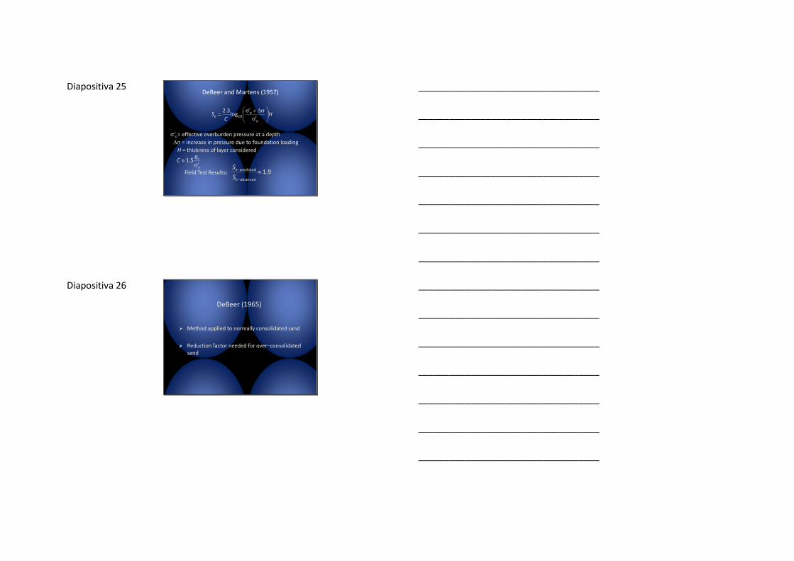
Diapositiva 25 DeBeer and Martens (1957)
‘o= effective overburden pressure at a depth
= increase in pressure due to foundation loading
H = thickness of layer considered
Field Test Results:
HC
So
oe
10log
3.2
o
cqC
5.1
9.1observed
predicted
e
e
S
S
___________________________________
___________________________________
___________________________________
___________________________________
___________________________________
___________________________________
___________________________________
Diapositiva 26
DeBeer (1965)
Method applied to normally consolidated sand
Reduction factor needed for over−consolidated sand
___________________________________
___________________________________
___________________________________
___________________________________
___________________________________
___________________________________
___________________________________
Diapositiva 27
Hough (1969)
)(
log1
10
beaC
He
CS
oc
o
o
o
ce
___________________________________
___________________________________
___________________________________
___________________________________
___________________________________
___________________________________
___________________________________
Diapositiva 28
Type of soil
Value ofconstant
a b
Uniform cohesionless material(uniformity coefficient Cu ≤ 2)
Well-graded cohesionless soilSilty sand and gravelClean, coarse to fine sandCoarse to fine silty sandSandy silt (inorganic)
0.090.120.150.18
0.200.350.250.25
___________________________________
___________________________________
___________________________________
___________________________________
___________________________________
___________________________________
___________________________________
Diapositiva 29 Peck and Bazaraa (1969)
where B is in m
(N1)60 = corrected standard penetration number
CW = ‘o /o at 0.5B below the bottom of foundation
o = total overburden pressure
‘o = effective overburden pressure
CD = 1.0 – 0.4(D/q) 0.5
= unit weight of soil
3.0)(
)(kN/m2(mm)
2
601
2
B
B
N
qCCS DWe
___________________________________
___________________________________
___________________________________
___________________________________
___________________________________
___________________________________
___________________________________
Diapositiva 30
Peck and Bazaraa (1969)
)kN/m 75( 01.025.3
4)( 260601
o
o
NN
)kN/m 75( 04.01
4)( 260601
o
o
NN
___________________________________
___________________________________
___________________________________
___________________________________
___________________________________
___________________________________
___________________________________
Diapositiva 31 Peck and Bazaraa’s Method(after D’Appolonia et al. 1970)
___________________________________
___________________________________
___________________________________
___________________________________
___________________________________
___________________________________
___________________________________
Diapositiva 32 GRANULAR SOIL
Burland and Burbidge (1985)
where N60(a) = adjusted N60 value
60)(60 25.1 gravel sandyor gravel For
NN a
)15(6.015
15 andwater ground the
below sand siltyor sand fine For
60)(60
60
NN
Na
___________________________________
___________________________________
___________________________________
___________________________________
___________________________________
___________________________________
___________________________________
Diapositiva 33 Depth of Stress Influence, z'
If N60(a) [or N60(a)] is approximately constant (or increasing) with depth,
where
BR = reference width = 0.3m
B = width of the actual foundation (m)
75.0
4.1
RR B
B
B
z
___________________________________
___________________________________
___________________________________
___________________________________
___________________________________
___________________________________
___________________________________
Diapositiva 34
Depth of Stress Influence, z'
If N60(a) [or N60(a)] is decreasing with depth, calculate z‘ = 2B and z‘ = distance from the bottom of the foundation to the bottom of the soft soil layer (z“ ).
Use z‘ = 2B or z‘ = z“, whichever is smaller.
___________________________________
___________________________________
___________________________________
___________________________________
___________________________________
___________________________________
___________________________________
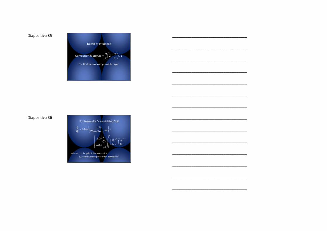
Diapositiva 35
Depth of Influence
H = thickness of compressible layer
12 factor, Correction
z
H
z
H
___________________________________
___________________________________
___________________________________
___________________________________
___________________________________
___________________________________
___________________________________
Diapositiva 36 For Normally Consolidated Soil
where L = length of the foundation
pa = atmospheric pressure (= 100 kN/m2)
aR
aR
e
p
q
B
B
B
LB
L
NNB
S
7.0
2
4.1)(6060
25.0
25.1
] or [
71.114.0
___________________________________
___________________________________
___________________________________
___________________________________
___________________________________
___________________________________
___________________________________
Diapositiva 37 For Overconsolidated Soil
pressure) idationoverconsol ;( ccq
aR
aR
e
p
q
B
B
B
LB
L
NNB
S
7.0
2
4.1)(6060
25.0
25.1
] or [
57.0447.0
___________________________________
___________________________________
___________________________________
___________________________________
___________________________________
___________________________________
___________________________________
Diapositiva 38 For Overconsolidated Soil
:)( cq
a
c
R
aR
e
p
q
B
B
B
LB
L
NNB
S
67.0
25.0
25.1
] or [
57.014.0
7.0
2
4.1)(6060
___________________________________
___________________________________
___________________________________
___________________________________
___________________________________
___________________________________
___________________________________
Diapositiva 39 Probability of Exceeding 25-mm Settlement in the Field(After Sivakugan and Johnson 2004)
Predictedsettlement
(mm)
Predicted methods
Terzaghi & Peck (1948)
Schmertmann(1970)
Burland &Burbidge
(1985)
15
10152025303540
0.000.000.000.090.200.260.310.35
0.387
0.000.000.020.130.200.270.320.370.42
0.000.030.150.250.340.420.490.440.51
___________________________________
___________________________________
___________________________________
___________________________________
___________________________________
___________________________________
___________________________________
Diapositiva 40
CATEGORY B
Schmertmann (1970),
Schmertmann et al. (1978)
Briaud (2007)
Terzaghi, Peck and Mesri (1996)
Akbas and Kulhawy (2009)
___________________________________
___________________________________
___________________________________
___________________________________
___________________________________
___________________________________
___________________________________
Diapositiva 41
Schmertmann (1970)
])21)[(1(
])21[()1(
BAq
EI
BAE
q
sssz
z
ss
sz
___________________________________
___________________________________
___________________________________
___________________________________
___________________________________
___________________________________
___________________________________
Diapositiva 42
___________________________________
___________________________________
___________________________________
___________________________________
___________________________________
___________________________________
___________________________________
Diapositiva 43
q = net stress at the level of the foundation
C 1 = correction factor for the depth of the foundation= 1 – 0.5(qo /q)
qo = effective overburden pressure at the level of thefoundation
C 2 = correction factor to account for creep in soil
= 1+0.2 log(t/0.1)
Es = 2qc
zE
IqCCS
s
ze 21
___________________________________
___________________________________
___________________________________
___________________________________
___________________________________
___________________________________
___________________________________
Diapositiva 44
The same 79 foundations records
given by Jeypalan and Boehm (1986)
and Papadopoulos (1992)
were analyzed by
Sivakugan et al. (1998).
___________________________________
___________________________________
___________________________________
___________________________________
___________________________________
___________________________________
___________________________________
Diapositiva 45
___________________________________
___________________________________
___________________________________
___________________________________
___________________________________
___________________________________
___________________________________
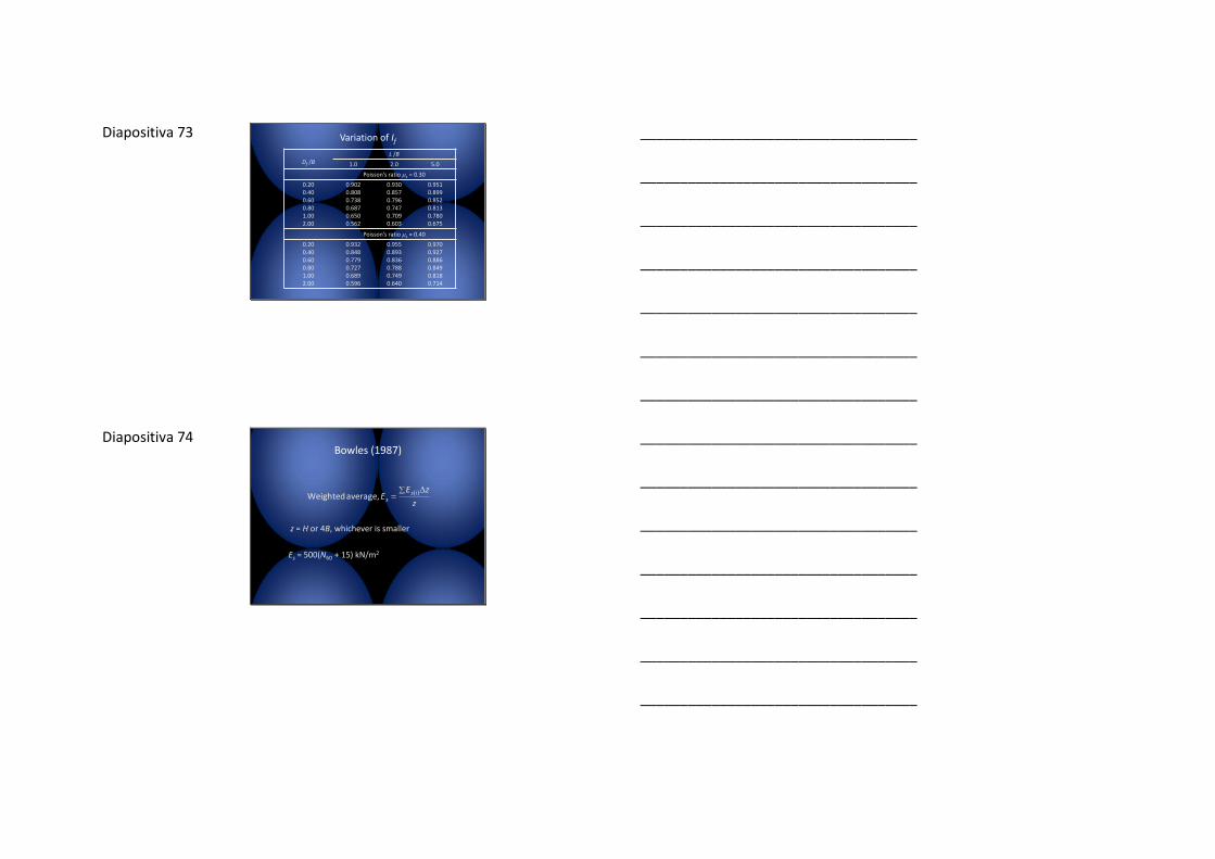
Diapositiva 46 Schmertmann et al. (1978)
Item L/B = 1 L/B 10
Iz at z = 0 0.1 0.2
zp /B 0.5 1.0
zo /B 2.0 4.0
Es 2.5qc 3.5qc
5.0
(peak) 1.05.0
oz
qI
___________________________________
___________________________________
___________________________________
___________________________________
___________________________________
___________________________________
___________________________________
Diapositiva 47
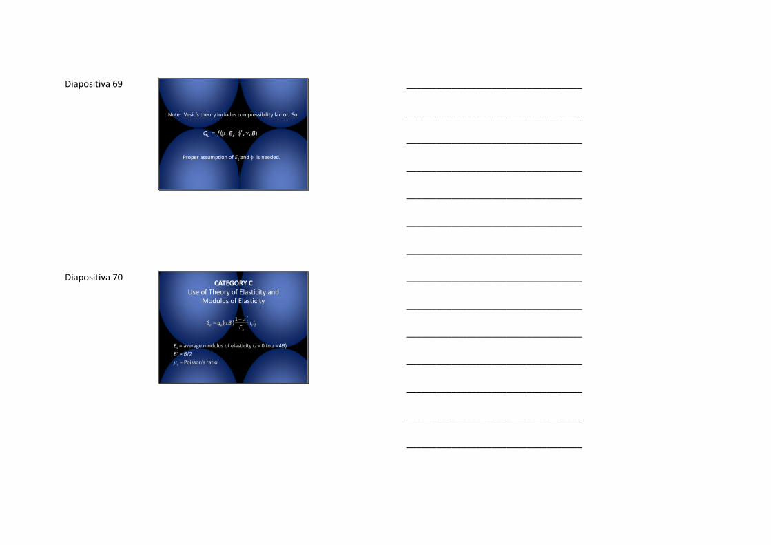
Salgado (2008)
41222.02
110555.05.0
20111.01.0)0 (at
B
L
B
z
B
L
B
z
B
LI
o
p
zz
___________________________________
___________________________________
___________________________________
___________________________________
___________________________________
___________________________________
___________________________________
Diapositiva 48 Lee et al. (2008)
FEM Analysis
6 at 4of maximum a with
4315
cos95.0
6at 1of maximum a with
1111.05.0
5.0)(peak
B
LB
L
B
z
B
LB
L
B
z
I
o
p
z
___________________________________
___________________________________
___________________________________
___________________________________
___________________________________
___________________________________
___________________________________
Diapositiva 49
Terzaghi et al.(1996)
4log12
B
Lzo
___________________________________
___________________________________
___________________________________
___________________________________
___________________________________
___________________________________
___________________________________
Diapositiva 50
___________________________________
___________________________________
___________________________________
___________________________________
___________________________________
___________________________________
___________________________________
Diapositiva 51
)MN/m (in value mean weighted
day 1days
log1.0
5.3
4.1log4.01
2
(creep)
)1/(
)1/(
)/(
0
cc
oc
e
cBLs
BLs
BLs
zz
z s
ze
qq
tz
qS
qE
BL
E
E
zEI
qSo
___________________________________
___________________________________
___________________________________
___________________________________
___________________________________
___________________________________
___________________________________
Diapositiva 52
___________________________________
___________________________________
___________________________________
___________________________________
___________________________________
___________________________________
___________________________________
Diapositiva 53 81 Foundation and 92 Plate Load Tests
1. Meyerhof’s relations (1965) simple to use. On the average, will give Se(predicted)/Se(observed) 1.5 to 2.0.
2. Peck & Bazaraa method (1969) is not superior to that of Meyerhof (1965).
3. Burland & Burbidge (1965) is an improved method over that of Meyerhof (1965) and Peck & Bazaraa (1969).
Difficult to estimate overconsolidation pressure from field exploration.
___________________________________
___________________________________
___________________________________
___________________________________
___________________________________
___________________________________
___________________________________
Diapositiva 91 4. Modified strain influence factor methods of
Schmertmann et al. (1978), Terzaghi et al. (1996), Salgado (2008) and Lee et al. (2008) will give reasonable results with proper values of Es .
5. Suggested Es relations:
6. The Es (L/B = 1) relationship can be related to N60 via D50 .
cBLs
BLs
BLs
qE
B
L
E
E
5.3
4.1log4.01
)1/(
)1/(
)/(
___________________________________
___________________________________
___________________________________
___________________________________
___________________________________
___________________________________
___________________________________
Diapositiva 92 7. Pressuremeter method of developing load-
settlement relationship is very effective, but may not be cost effective.
8. L1 – L2 (Akbas and Kulhawy) is a good method. However proper assumption of E and needed to estimate QL2.
9. Relationships for settlement developed using theory of elasticity will give equally good results provided a realistic Es is used. Use of iteration method is suggested.
If not, used Terzaghi et al.’s relationship (1996).
___________________________________
___________________________________
___________________________________
___________________________________
___________________________________
___________________________________
___________________________________
Diapositiva 93
___________________________________
___________________________________
___________________________________
___________________________________
___________________________________
___________________________________
___________________________________
Diapositiva 94
___________________________________
___________________________________
___________________________________
___________________________________
___________________________________
___________________________________
___________________________________
Diapositiva 95
What we have seen is a systematic
accumulation of knowledge over 60 years.
The parameters for comparing settlement
prediction methods are accuracy and
reliability.
Reliability is the probability that the actual
settlement would be less than that computed
by a specific method.
___________________________________
___________________________________
___________________________________
___________________________________
___________________________________
___________________________________
___________________________________
Diapositiva 96 In choosing a method for design, it all comes
down to keeping a critical balance between reliability and accuracy, which can be difficult at times, knowing the non-homogeneous nature of soil in general. We cannot be over-conservative but, at the same time, not be accurate.
We need to keep in mind what Karl Terzaghi said in the 45th James Forrest Lecture at the Institute of Civil Engineers in London: “Foundation failures that occur are no longer‘an act of God’.”


![The shallow elastic structure of the lunar crust: New ...jupiter.ethz.ch/~akhan/amir/Publications_files/sollberger_etal_grl16.pdf · [Horvathetal., 1980] and by laboratory experiments](https://static.documents.pub/doc/80x56/5e6cd691b035d5735f7264ce/the-shallow-elastic-structure-of-the-lunar-crust-new-akhanamirpublicationsfilessollbergeretalgrl16pdf.jpg)