ElasticTree: Saving Energy in Data Center Networks

Brandon Heller⋆, Srini Seetharaman†, Priya Mahadevan⋄,Yiannis Yiakoumis⋆, Puneet Sharma⋄, Sujata Banerjee⋄, Nick McKeown⋆

⋆ Stanford University, Palo Alto, CA USA† Deutsche Telekom R&D Lab, Los Altos, CA USA

⋄ Hewlett-Packard Labs, Palo Alto, CA USA

ABSTRACT

Networks are a shared resource connecting critical IT in-

frastructure, and the general practice is to always leave

them on. Yet, meaningful energy savings can result from

improving a network’s ability to scale up and down, as

traffic demands ebb and flow. We present ElasticTree, a

network-wide power1 manager, which dynamically ad-

justs the set of active network elements — links and

switches — to satisfy changing data center traffic loads.

We first compare multiple strategies for finding

minimum-power network subsets across a range of traf-

fic patterns. We implement and analyze ElasticTree

on a prototype testbed built with production OpenFlow

switches from three network vendors. Further, we ex-

amine the trade-offs between energy efficiency, perfor-

mance and robustness, with real traces from a produc-

tion e-commerce website. Our results demonstrate that

for data center workloads, ElasticTree can save up to

50% of network energy, while maintaining the ability to

handle traffic surges. Our fast heuristic for computing

network subsets enables ElasticTree to scale to data cen-

ters containing thousands of nodes. We finish by show-

ing how a network admin might configure ElasticTree to

satisfy their needs for performance and fault tolerance,

while minimizing their network power bill.

1. INTRODUCTION

Data centers aim to provide reliable and scalablecomputing infrastructure for massive Internet ser-vices. To achieve these properties, they consumehuge amounts of energy, and the resulting opera-tional costs have spurred interest in improving theirefficiency. Most efforts have focused on servers andcooling, which account for about 70% of a data cen-ter’s total power budget. Improvements include bet-ter components (low-power CPUs [12], more effi-cient power supplies and water-cooling) as well asbetter software (tickless kernel, virtualization, andsmart cooling [30]).

With energy management schemes for the largestpower consumers well in place, we turn to a part ofthe data center that consumes 10-20% of its total

1We use power and energy interchangeably in this paper.

power: the network [9]. The total power consumedby networking elements in data centers in 2006 inthe U.S. alone was 3 billion kWh and rising [7]; ourgoal is to significantly reduce this rapidly growingenergy cost.

1.1 Data Center Networks

As services scale beyond ten thousand servers,inflexibility and insufficient bisection bandwidthhave prompted researchers to explore alternativesto the traditional 2N tree topology (shown in Fig-ure 1(a)) [1] with designs such as VL2 [10], Port-Land [24], DCell [16], and BCube [15]. The re-sulting networks look more like a mesh than a tree.One such example, the fat tree [1]2, seen in Figure1(b), is built from a large number of richly connectedswitches, and can support any communication pat-tern (i.e. full bisection bandwidth). Traffic fromlower layers is spread across the core, using multi-path routing, valiant load balancing, or a number ofother techniques.

In a 2N tree, one failure can cut the effective bi-section bandwidth in half, while two failures can dis-connect servers. Richer, mesh-like topologies handlefailures more gracefully; with more components andmore paths, the effect of any individual componentfailure becomes manageable. This property can alsohelp improve energy efficiency. In fact, dynamicallyvarying the number of active (powered on) networkelements provides a control knob to tune betweenenergy efficiency, performance, and fault tolerance,which we explore in the rest of this paper.

1.2 Inside a Data Center

Data centers are typically provisioned for peakworkload, and run well below capacity most of thetime. Traffic varies daily (e.g., email checking duringthe day), weekly (e.g., enterprise database querieson weekdays), monthly (e.g., photo sharing on holi-days), and yearly (e.g., more shopping in December).Rare events like cable cuts or celebrity news may hitthe peak capacity, but most of the time traffic canbe satisfied by a subset of the network links and

2Essentially a buffered Clos topology.

1

(a) Typical Data Center Network.Racks hold up to 40 “1U” servers, andtwo edge switches (i.e.“top-of-rack”switches.)

(b) Fat tree. All 1G links, always on. (c) Elastic Tree. 0.2 Gbps per hostacross data center can be satisfied by afat tree subset (here, a spanning tree),yielding 38% savings.

Figure 1: Data Center Networks: (a), 2N Tree (b), Fat Tree (c), ElasticTree

0

5

10

15

20

0 100 200 300 400 500 600 700 800 0

1000

2000

3000

4000

5000

6000

7000

8000

Ba

nd

wid

th in

Gb

ps

Po

we

r in

Wa

tts

Time (1 unit = 10 mins)

Total Traffic in Gbps

PowerTraffic

Figure 2: E-commerce website: 292 produc-tion web servers over 5 days. Traffic variesby day/weekend, power doesn’t.

switches. These observations are based on tracescollected from two production data centers.

Trace 1 (Figure 2) shows aggregate traffic col-lected from 292 servers hosting an e-commerce ap-plication over a 5 day period in April 2008 [22]. Aclear diurnal pattern emerges; traffic peaks duringthe day and falls at night. Even though the trafficvaries significantly with time, the rack and aggre-gation switches associated with these servers drawconstant power (secondary axis in Figure 2).

Trace 2 (Figure 3) shows input and output trafficat a router port in a production Google data centerin September 2009. The Y axis is in Mbps. The 8-day trace shows diurnal and weekend/weekday vari-ation, along with a constant amount of backgroundtraffic. The 1-day trace highlights more short-termbursts. Here, as in the previous case, the powerconsumed by the router is fixed, irrespective of thetraffic through it.

1.3 Energy Proportionality

An earlier power measurement study [22] had pre-sented power consumption numbers for several datacenter switches for a variety of traffic patterns and

(a) Router port for 8 days. Input/output ratio varies.

(b) Router port from Sunday to Monday. Notemarked increase and short-term spikes.

Figure 3: Google Production Data Center

switch configurations. We use switch power mea-surements from this study and summarize relevantresults in Table 1. In all cases, turning the switch onconsumes most of the power; going from zero to fulltraffic increases power by less than 8%. Turning off aswitch yields the most power benefits, while turningoff an unused port saves only 1-2 Watts. Ideally, anunused switch would consume no power, and energyusage would grow with increasing traffic load. Con-suming energy in proportion to the load is a highlydesirable behavior [4, 22].

Unfortunately, today’s network elements are notenergy proportional: fixed overheads such as fans,switch chips, and transceivers waste power at lowloads. The situation is improving, as competitionencourages more efficient products, such as closer-to-energy-proportional links and switches [19, 18,26, 14]. However, maximum efficiency comes from a

2

Ports Port Model A Model B Model CEnabled Traffic power (W) power (W) power (W)

None None 151 133 76All None 184 170 97All 1 Gbps 195 175 102

Table 1: Power consumption of various 48-port switches for different configurations

combination of improved components and improvedcomponent management.

Our choice – as presented in this paper – is tomanage today’s non energy-proportional networkcomponents more intelligently. By zooming out toa whole-data-center view, a network of on-or-off,non-proportional components can act as an energy-proportional ensemble, and adapt to varying trafficloads. The strategy is simple: turn off the links andswitches that we don’t need, right now, to keep avail-able only as much networking capacity as required.

1.4 Our Approach

ElasticTree is a network-wide energy optimizerthat continuously monitors data center traffic con-ditions. It chooses the set of network elements thatmust stay active to meet performance and fault tol-erance goals; then it powers down as many unneededlinks and switches as possible. We use a variety ofmethods to decide which subset of links and switchesto use, including a formal model, greedy bin-packer,topology-aware heuristic, and prediction methods.We evaluate ElasticTree by using it to control thenetwork of a purpose-built cluster of computers andswitches designed to represent a data center. Notethat our approach applies to currently-deployed net-work devices, as well as newer, more energy-efficientones. It applies to single forwarding boxes in a net-work, as well as individual switch chips within alarge chassis-based router.

While the energy savings from powering off anindividual switch might seem insignificant, a largedata center hosting hundreds of thousands of serverswill have tens of thousands of switches deployed.The energy savings depend on the traffic patterns,the level of desired system redundancy, and the sizeof the data center itself. Our experiments show that,on average, savings of 25-40% of the network en-ergy in data centers is feasible. Extrapolating to alldata centers in the U.S., we estimate the savings tobe about 1 billion KWhr annually (based on 3 bil-lion kWh used by networking devices in U.S. datacenters [7]). Additionally, reducing the energy con-sumed by networking devices also results in a pro-portional reduction in cooling costs.

Figure 4: System Diagram

The remainder of the paper is organized as fol-lows: §2 describes in more detail the ElasticTreeapproach, plus the modules used to build the pro-totype. §3 computes the power savings possible fordifferent communication patterns to understand bestand worse-case scenarios. We also explore powersavings using real data center traffic traces. In §4,we measure the potential impact on bandwidth andlatency due to ElasticTree. In §5, we explore deploy-ment aspects of ElasticTree in a real data center.We present related work in §6 and discuss lessonslearned in §7.

2. ELASTICTREE

ElasticTree is a system for dynamically adaptingthe energy consumption of a data center network.ElasticTree consists of three logical modules - opti-mizer, routing, and power control - as shown in Fig-ure 4. The optimizer’s role is to find the minimum-power network subset which satisfies current trafficconditions. Its inputs are the topology, traffic ma-trix, a power model for each switch, and the desiredfault tolerance properties (spare switches and sparecapacity). The optimizer outputs a set of activecomponents to both the power control and routingmodules. Power control toggles the power states ofports, linecards, and entire switches, while routingchooses paths for all flows, then pushes routes intothe network.

We now show an example of the system in action.

2.1 Example

Figure 1(c) shows a worst-case pattern for networklocality, where each host sends one data flow halfwayacross the data center. In this example, 0.2 Gbpsof traffic per host must traverse the network core.When the optimizer sees this traffic pattern, it findswhich subset of the network is sufficient to satisfythe traffic matrix. In fact, a minimum spanning tree(MST) is sufficient, and leaves 0.2 Gbps of extracapacity along each core link. The optimizer then

3

informs the routing module to compress traffic alongthe new sub-topology, and finally informs the powercontrol module to turn off unneeded switches andlinks. We assume a 3:1 idle:active ratio for modelingswitch power consumption; that is, 3W of power tohave a switch port, and 1W extra to turn it on, basedon the 48-port switch measurements shown in Table1. In this example, 13/20 switches and 28/48 linksstay active, and ElasticTree reduces network powerby 38%.

As traffic conditions change, the optimizer con-tinuously recomputes the optimal network subset.As traffic increases, more capacity is brought online,until the full network capacity is reached. As trafficdecreases, switches and links are turned off. Notethat when traffic is increasing, the system must waitfor capacity to come online before routing throughthat capacity. In the other direction, when trafficis decreasing, the system must change the routing- by moving flows off of soon-to-be-down links andswitches - before power control can shut anythingdown.

Of course, this example goes too far in the direc-tion of power efficiency. The MST solution leaves thenetwork prone to disconnection from a single failedlink or switch, and provides little extra capacity toabsorb additional traffic. Furthermore, a networkoperated close to its capacity will increase the chanceof dropped and/or delayed packets. Later sectionsexplore the tradeoffs between power, fault tolerance,and performance. Simple modifications can dramat-ically improve fault tolerance and performance atlow power, especially for larger networks. We nowdescribe each of ElasticTree modules in detail.

2.2 Optimizers

We have developed a range of methods to com-pute a minimum-power network subset in Elastic-Tree, as summarized in Table 2. The first method isa formal model, mainly used to evaluate the solutionquality of other optimizers, due to heavy computa-tional requirements. The second method is greedybin-packing, useful for understanding power savingsfor larger topologies. The third method is a simpleheuristic to quickly find subsets in networks withregular structure. Each method achieves differenttradeoffs between scalability and optimality. Allmethods can be improved by considering a data cen-ter’s past traffic history (details in §5.4).

2.2.1 Formal Model

We desire the optimal-power solution (subset andflow assignment) that satisfies the traffic constraints,3Bounded percentage from optimal, configured to 10%.

Type Quality Scalability Input Topo

Formal Optimal 3 Low Traffic Matrix Any

Greedy Good Medium Traffic Matrix Any

Topo- OK High Port Counters Fat

aware Tree

Table 2: Optimizer Comparison

but finding the optimal flow assignment alone is anNP-complete problem for integer flows. Despite thiscomputational complexity, the formal model pro-vides a valuable tool for understanding the solutionquality of other optimizers. It is flexible enough tosupport arbitrary topologies, but can only scale upto networks with less than 1000 nodes.

The model starts with a standard multi-commodity flow (MCF) problem. For the preciseMCF formulation, see Appendix A. The constraintsinclude link capacity, flow conservation, and demandsatisfaction. The variables are the flows along eachlink. The inputs include the topology, switch powermodel, and traffic matrix. To optimize for power, weadd binary variables for every link and switch, andconstrain traffic to only active (powered on) linksand switches. The model also ensures that the fullpower cost for an Ethernet link is incurred when ei-ther side is transmitting; there is no such thing as ahalf-on Ethernet link.

The optimization goal is to minimize the total net-work power, while satisfying all constraints. Split-ting a single flow across multiple links in the topol-ogy might reduce power by improving link utilizationoverall, but reordered packets at the destination (re-sulting from varying path delays) will negatively im-pact TCP performance. Therefore, we include con-straints in our formulation to (optionally) preventflows from getting split.

The model outputs a subset of the original topol-ogy, plus the routes taken by each flow to satisfythe traffic matrix. Our model shares similar goals toChabarek et al. [6], which also looked at power-awarerouting. However, our model (1) focuses on datacenters, not wide-area networks, (2) chooses a sub-set of a fixed topology, not the component (switch)configurations in a topology, and (3) considers indi-vidual flows, rather than aggregate traffic.

We implement our formal method using bothMathProg and General Algebraic Modeling System(GAMS), which are high-level languages for opti-mization modeling. We use both the GNU LinearProgramming Kit (GLPK) and CPLEX to solve theformulation.

4

2.2.2 Greedy Bin-Packing

For even simple traffic patterns, the formalmodel’s solution time scales to the 3.5th power as afunction of the number of hosts (details in §5). Thegreedy bin-packing heuristic improves on the formalmodel’s scalability. Solutions within a bound of opti-mal are not guaranteed, but in practice, high-qualitysubsets result. For each flow, the greedy bin-packerevaluates possible paths and chooses the leftmostone with sufficient capacity. By leftmost, we meanin reference to a single layer in a structured topol-ogy, such as a fat tree. Within a layer, paths arechosen in a deterministic left-to-right order, as op-posed to a random order, which would evenly spreadflows. When all flows have been assigned (which isnot guaranteed), the algorithm returns the activenetwork subset (set of switches and links traversedby some flow) plus each flow path.

For some traffic matrices, the greedy approach willnot find a satisfying assignment for all flows; thisis an inherent problem with any greedy flow assign-ment strategy, even when the network is provisionedfor full bisection bandwidth. In this case, the greedysearch will have enumerated all possible paths, andthe flow will be assigned to the path with the lowestload. Like the model, this approach requires knowl-edge of the traffic matrix, but the solution can becomputed incrementally, possibly to support on-lineusage.

2.2.3 Topology-aware Heuristic

The last method leverages the regularity of the fattree topology to quickly find network subsets. Unlikethe other methods, it does not compute the set offlow routes, and assumes perfectly divisible flows. Ofcourse, by splitting flows, it will pack every link tofull utilization and reduce TCP bandwidth — notexactly practical.

However, simple additions to this “starter sub-set” lead to solutions of comparable quality to othermethods, but computed with less information, andin a fraction of the time. In addition, by decouplingpower optimization from routing, our method canbe applied alongside any fat tree routing algorithm,including OSPF-ECMP, valiant load balancing [10],flow classification [1] [2], and end-host path selec-tion [23]. Computing this subset requires only portcounters, not a full traffic matrix.

The intuition behind our heuristic is that to satisfytraffic demands, an edge switch doesn’t care whichaggregation switches are active, but instead, how

many are active. The “view” of every edge switch ina given pod is identical; all see the same number ofaggregation switches above. The number of required

switches in the aggregation layer is then equal to thenumber of links required to support the traffic ofthe most active source above or below (whichever ishigher), assuming flows are perfectly divisible. Forexample, if the most active source sends 2 Gbps oftraffic up to the aggregation layer and each link is1 Gbps, then two aggregation layer switches muststay on to satisfy that demand. A similar observa-tion holds between each pod and the core, and theexact subset computation is described in more detailin §5. One can think of the topology-aware heuristicas a cron job for that network, providing periodicinput to any fat tree routing algorithm.

For simplicity, our computations assume a homo-geneous fat tree with one link between every con-nected pair of switches. However, this techniqueapplies to full-bisection-bandwidth topologies withany number of layers (we show only 3 stages), bun-dled links (parallel links connecting two switches),or varying speeds. Extra “switches at a given layer”computations must be added for topologies withmore layers. Bundled links can be considered sin-gle faster links. The same computation works forother topologies, such as the aggregated Clos usedby VL2 [10], which has 10G links above the edgelayer and 1G links to each host.

We have implemented all three optimizers; eachoutputs a network topology subset, which is thenused by the control software.

2.3 Control Software

ElasticTree requires two network capabilities:traffic data (current network utilization) and controlover flow paths. NetFlow [27], SNMP and samplingcan provide traffic data, while policy-based rout-ing can provide path control, to some extent. Inour ElasticTree prototype, we use OpenFlow [29] toachieve the above tasks.

OpenFlow: OpenFlow is an open API addedto commercial switches and routers that provides aflow table abstraction. We first use OpenFlow tovalidate optimizer solutions by directly pushing thecomputed set of application-level flow routes to eachswitch, then generating traffic as described later inthis section. In the live prototype, OpenFlow alsoprovides the traffic matrix (flow-specific counters),port counters, and port power control. OpenFlowenables us to evaluate ElasticTree on switches fromdifferent vendors, with no source code changes.

NOX: NOX is a centralized platform that pro-vides network visibility and control atop a networkof OpenFlow switches [13]. The logical modulesin ElasticTree are implemented as a NOX applica-tion. The application pulls flow and port counters,

5

Figure 5: Hardware Testbed (HP switch fork = 6 fat tree)

Vendor Model k Virtual Switches Ports Hosts

HP 5400 6 45 270 54Quanta LB4G 4 20 80 16NEC IP8800 4 20 80 16

Table 3: Fat Tree Configurations

directs these to an optimizer, and then adjusts flowroutes and port status based on the computed sub-set. In our current setup, we do not power off in-active switches, due to the fact that our switchesare virtual switches. However, in a real data cen-ter deployment, we can leverage any of the existingmechanisms such as command line interface, SNMPor newer control mechanisms such as power-controlover OpenFlow in order to support the power controlfeatures.

2.4 Prototype Testbed

We build multiple testbeds to verify and evaluateElasticTree, summarized in Table 3, with an exam-ple shown in Figure 5. Each configuration multi-plexes many smaller virtual switches (with 4 or 6ports) onto one or more large physical switches. Allcommunication between virtual switches is done overdirect links (not through any switch backplane or in-termediate switch).

The smaller configuration is a complete k = 4three-layer homogeneous fat tree4, split into 20 in-dependent four-port virtual switches, supporting 16nodes at 1 Gbps apiece. One instantiation com-prised 2 NEC IP8800 24-port switches and 1 48-port switch, running OpenFlow v0.8.9 firmware pro-vided by NEC Labs. Another comprised two QuantaLB4G 48-port switches, running the OpenFlow Ref-erence Broadcom firmware.

4Refer [1] for details on fat trees and definition of k

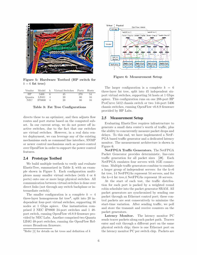
Figure 6: Measurement Setup

The larger configuration is a complete k = 6three-layer fat tree, split into 45 independent six-port virtual switches, supporting 54 hosts at 1 Gbpsapiece. This configuration runs on one 288-port HPProCurve 5412 chassis switch or two 144-port 5406chassis switches, running OpenFlow v0.8.9 firmwareprovided by HP Labs.

2.5 Measurement Setup

Evaluating ElasticTree requires infrastructure togenerate a small data center’s worth of traffic, plusthe ability to concurrently measure packet drops anddelays. To this end, we have implemented a NetF-PGA based traffic generator and a dedicated latencymonitor. The measurement architecture is shown inFigure 6.

NetFPGA Traffic Generators. The NetFPGAPacket Generator provides deterministic, line-ratetraffic generation for all packet sizes [28]. EachNetFPGA emulates four servers with 1GE connec-tions. Multiple traffic generators combine to emulatea larger group of independent servers: for the k=6fat tree, 14 NetFPGAs represent 54 servers, and forthe k=4 fat tree,4 NetFPGAs represent 16 servers.

At the start of each test, the traffic distribu-tion for each port is packed by a weighted roundrobin scheduler into the packet generator SRAM. Allpacket generators are synchronized by sending onepacket through an Ethernet control port; these con-trol packets are sent consecutively to minimize thestart-time variation. After sending traffic, we polland store the transmit and receive counters on thepacket generators.

Latency Monitor. The latency monitor PCsends tracer packets along each packet path. Tracersenter and exit through a different port on the samephysical switch chip; there is one Ethernet port onthe latency monitor PC per switch chip. Packets are

6

logged by Pcap on entry and exit to record precisetimestamp deltas. We report median figures that areaveraged over all packet paths. To ensure measure-ments are taken in steady state, the latency moni-tor starts up after 100 ms. This technique capturesall but the last-hop egress queuing delays. Sinceedge links are never oversubscribed for our trafficpatterns, the last-hop egress queue should incur noadded delay.

3. POWER SAVINGS ANALYSIS

In this section, we analyze ElasticTree’s networkenergy savings when compared to an always-on base-line. Our comparisons assume a homogeneous fattree for simplicity, though the evaluation also appliesto full-bisection-bandwidth topologies with aggrega-tion, such as those with 1G links at the edge and10G at the core. The primary metric we inspect is% original network power, computed as:

=Power consumed by ElasticTree× 100

Power consumed by original fat-tree

This percentage gives an accurate idea of the over-all power saved by turning off switches and links(i.e., savings equal 100 - % original power). Weuse power numbers from switch model A (§1.3) forboth the baseline and ElasticTree cases, and onlyinclude active (powered-on) switches and links forElasticTree cases. Since all three switches in Ta-ble 1 have an idle:active ratio of 3:1 (explained in§2.1), using power numbers from switch model Bor C will yield similar network energy savings. Un-less otherwise noted, optimizer solutions come fromthe greedy bin-packing algorithm, with flow splittingdisabled (as explained in Section 2). We validate theresults for all k = {4, 6} fat tree topologies on mul-tiple testbeds. For all communication patterns, themeasured bandwidth as reported by receive countersmatches the expected values. We only report energysaved directly from the network; extra energy will berequired to power on and keep running the servershosting ElasticTree modules. There will be addi-tional energy required for cooling these servers, andat the same time, powering off unused switches willresult in cooling energy savings. We do not includethese extra costs/savings in this paper.

3.1 Traffic Patterns

Energy, performance and robustness all dependheavily on the traffic pattern. We now explore thepossible energy savings over a wide range of commu-nication patterns, leaving performance and robust-ness for §4.

0.0 0.2 0.4 0.6 0.8 1.0Traffic Demand (Gbps)

0

20

40

60

80

100

% o

rigin

al netw

ork

pow

er

Far

50% Far, 50% Mid

Mid

50% Near, 50% Mid

Near

Figure 7: Power savings as a function of de-mand, with varying traffic locality, for a 28K-node, k=48 fat tree

3.1.1 Uniform Demand, Varying Locality

First, consider two extreme cases: near (highlylocalized) traffic matrices, where servers commu-nicate only with other servers through their edgeswitch, and far (non-localized) traffic matriceswhere servers communicate only with servers inother pods, through the network core. In this pat-tern, all traffic stays within the data center, andnone comes from outside. Understanding these ex-treme cases helps to quantify the range of networkenergy savings. Here, we use the formal method asthe optimizer in ElasticTree.

Near traffic is a best-case — leading to the largestenergy savings — because ElasticTree will reducethe network to the minimum spanning tree, switch-ing off all but one core switch and one aggregationswitch per pod. On the other hand, far traffic is aworst-case — leading to the smallest energy savings— because every link and switch in the network isneeded. For far traffic, the savings depend heavily

on the network utilization, u =P

i

P

jλij

Total hosts (λij is thetraffic from host i to host j, λij < 1 Gbps). If u isclose to 100%, then all links and switches must re-main active. However, with lower utilization, trafficcan be concentrated onto a smaller number of corelinks, and unused ones switch off. Figure 7 showsthe potential savings as a function of utilization forboth extremes, as well as traffic to the aggregationlayer Mid), for a k = 48 fat tree with roughly 28Kservers. Running ElasticTree on this configuration,with near traffic at low utilization, we expect a net-work energy reduction of 60%; we cannot save anyfurther energy, as the active network subset in thiscase is the MST. For far traffic and u=100%, thereare no energy savings. This graph highlights thepower benefit of local communications, but more im-

7

0.0 0.1 0.2 0.3 0.4 0.5 0.6 0.7Avg. network utilization

0

20

40

60

80

100%

ori

gin

al netw

ork

pow

er

Figure 8: Scatterplot of power savings withrandom traffic matrix. Each point on thegraph corresponds to a pre-configured aver-age data center workload, for a k = 6 fat tree

portantly, shows potential savings in all cases. Hav-ing seen these two extremes, we now consider morerealistic traffic matrices with a mix of both near andfar traffic.

3.1.2 Random Demand

Here, we explore how much energy we can expectto save, on average, with random, admissible traf-fic matrices. Figure 8 shows energy saved by Elas-ticTree (relative to the baseline) for these matrices,generated by picking flows uniformly and randomly,then scaled down by the most oversubscribed host’straffic to ensure admissibility. As seen previously,for low utilization, ElasticTree saves roughly 60% ofthe network power, regardless of the traffic matrix.As the utilization increases, traffic matrices with sig-nificant amounts of far traffic will have less room forpower savings, and so the power saving decreases.The two large steps correspond to utilizations atwhich an extra aggregation switch becomes neces-sary across all pods. The smaller steps correspondto individual aggregation or core switches turning onand off. Some patterns will densely fill all availablelinks, while others will have to incur the entire powercost of a switch for a single link; hence the variabil-ity in some regions of the graph. Utilizations above0.75 are not shown; for these matrices, the greedybin-packer would sometimes fail to find a completesatisfying assignment of flows to links.

3.1.3 Sine-wave Demand

As seen before (§1.2), the utilization of a data cen-ter will vary over time, on daily, seasonal and annual

Figure 9: Power savings for sinusoidal trafficvariation in a k = 4 fat tree topology, with 1flow per host in the traffic matrix. The inputdemand has 10 discrete values.

time scales. Figure 9 shows a time-varying utiliza-tion; power savings from ElasticTree that follow theutilization curve. To crudely approximate diurnalvariation, we assume u = 1/2(1 + sin(t)), at time t,suitably scaled to repeat once per day. For this sinewave pattern of traffic demand, the network powercan be reduced up to 64% of the original power con-sumed, without being over-subscribed and causingcongestion.

We note that most energy savings in all the abovecommunication patterns comes from powering offswitches. Current networking devices are far frombeing energy proportional, with even completely idleswitches (0% utilization) consuming 70-80% of theirfully loaded power (100% utilization) [22]; thus pow-ering off switches yields the most energy savings.

3.1.4 Traffic in a Realistic Data Center

In order to evaluate energy savings with a realdata center workload, we collected system and net-work traces from a production data center hosting ane-commerce application (Trace 1, §1). The serversin the data center are organized in a tiered model asapplication servers, file servers and database servers.The System Activity Reporter (sar) toolkit availableon Linux obtains CPU, memory and network statis-tics, including the number of bytes transmitted andreceived from 292 servers. Our traces contain statis-tics averaged over a 10-minute interval and span 5days in April 2008. The aggregate traffic throughall the servers varies between 2 and 12 Gbps at anygiven time instant (Figure 2). Around 70% of the

8

0 100 200 300 400 500 600 700 800Time (1 unit = 10 mins)

0

20

40

60

80

100%

ori

gin

al netw

ork

pow

er

measured, 70% to Internet, x 20, greedy

measured, 70% to Internet, x 10, greedy

measured, 70% to Internet, x 1, greedy

Figure 10: Energy savings for productiondata center (e-commerce website) traces, overa 5 day period, using a k=12 fat tree. Weshow savings for different levels of overalltraffic, with 70% destined outside the DC.

traffic leaves the data center and the remaining 30%is distributed to servers within the data center.

In order to compute the energy savings from Elas-ticTree for these 292 hosts, we need a k = 12 fattree. Since our testbed only supports k = 4 andk = 6 sized fat trees, we simulate the effect of Elas-ticTree using the greedy bin-packing optimizer onthese traces. A fat tree with k = 12 can support upto 432 servers; since our traces are from 292 servers,we assume the remaining 140 servers have been pow-ered off. The edge switches associated with thesepowered-off servers are assumed to be powered off;we do not include their cost in the baseline routingpower calculation.

The e-commerce service does not generate enoughnetwork traffic to require a high bisection bandwidthtopology such as a fat tree. However, the time-varying characteristics are of interest for evaluatingElasticTree, and should remain valid with propor-tionally larger amounts of network traffic. Hence,we scale the traffic up by a factor of 20.

For different scaling factors, as well as for differentintra data center versus outside data center (exter-nal) traffic ratios, we observe energy savings rangingfrom 25-62%. We present our energy savings resultsin Figure 10. The main observation when visuallycomparing with Figure 2 is that the power consumedby the network follows the traffic load curve. Eventhough individual network devices are not energy-proportional, ElasticTree introduces energy propor-tionality into the network.

16 64 256 1024 4096 16384 65536# hosts in network

0

20

40

60

80

100

% o

rigin

al netw

ork

pow

er

MST+3

MST+2

MST+1

MST

Figure 11: Power cost of redundancy

0 20 40 60 80 100 120 140 160Time (1 unit = 10 mins)

40

45

50

55

60

65

70

% o

rigin

al netw

ork

pow

er

Statistics for Trace 1 for a day

70% to Internet, x 10, greedy

70% to Internet, x 10, greedy + 10% margin

70% to Internet, x 10, greedy + 20% margin

70% to Internet, x 10, greedy + 30% margin

70% to Internet, x 10, greedy + 1

70% to Internet, x 10, greedy + 2

70% to Internet, x 10, greedy + 3

Figure 12: Power consumption in a robustdata center network with safety margins, aswell as redundancy. Note “greedy+1” meanswe add a MST over the solution returned bythe greedy solver.

We stress that network energy savings are work-load dependent. While we have explored savingsin the best-case and worst-case traffic scenarios aswell as using traces from a production data center,a highly utilized and “never-idle” data center net-work would not benefit from running ElasticTree.

3.2 Robustness Analysis

Typically data center networks incorporate somelevel of capacity margin, as well as redundancy inthe topology, to prepare for traffic surges and net-work failures. In such cases, the network uses moreswitches and links than essential for the regular pro-duction workload.

Consider the case where only a minimum spanning

9

Figure 13: Queue Test Setups with one (left)and two (right) bottlenecks

tree (MST) in the fat tree topology is turned on (allother links/switches are powered off); this subsetcertainly minimizes power consumption. However,it also throws away all path redundancy, and withit, all fault tolerance. In Figure 11, we extend theMST in the fat tree with additional active switches,for varying topology sizes. The MST+1 configura-tion requires one additional edge switch per pod,and one additional switch in the core, to enable anysingle aggregation or core-level switch to fail with-out disconnecting a server. The MST+2 configura-tion enables any two failures in the core or aggre-gation layers, with no loss of connectivity. As thenetwork size increases, the incremental cost of addi-tional fault tolerance becomes an insignificant partof the total network power. For the largest networks,the savings reduce by only 1% for each additionalspanning tree in the core aggregation levels. Each+1 increment in redundancy has an additive cost,but a multiplicative benefit; with MST+2, for exam-ple, the failures would have to happen in the samepod to disconnect a host. This graph shows that theadded cost of fault tolerance is low.

Figure 12 presents power figures for the k=12 fattree topology when we add safety margins for ac-commodating bursts in the workload. We observethat the additional power cost incurred is minimal,while improving the network’s ability to absorb un-expected traffic surges.

4. PERFORMANCE

The power savings shown in the previous sectionare worthwhile only if the performance penalty isnegligible. In this section, we quantify the perfor-mance degradation from running traffic over a net-work subset, and show how to mitigate negative ef-fects with a safety margin.

4.1 Queuing Baseline

Figure 13 shows the setup for measuring the bufferdepth in our test switches; when queuing occurs,this knowledge helps to estimate the number of hopswhere packets are delayed. In the congestion-freecase (not shown), a dedicated latency monitor PCsends tracer packets into a switch, which sends itright back to the monitor. Packets are timestamped

Bottlenecks Median Std. Dev

0 36.00 2.94

1 473.97 7.12

2 914.45 10.50

Table 4: Latency baselines for Queue Test Se-tups

0.0 0.2 0.4 0.6 0.8 1.0Traffic demand (Gbps)

0

100

200

300

400

500

Late

ncy

media

nFigure 14: Latency vs demand, with uniformtraffic.

by the kernel, and we record the latency of each re-ceived packet, as well as the number of drops. Thistest is useful mainly to quantify PC-induced latencyvariability. In the single-bottleneck case, two hostssend 0.7 Gbps of constant-rate traffic to a singleswitch output port, which connects through a secondswitch to a receiver. Concurrently with the packetgenerator traffic, the latency monitor sends tracerpackets. In the double-bottleneck case, three hostssend 0.7 Gbps, again while tracers are sent.

Table 4 shows the latency distribution of tracerpackets sent through the Quanta switch, for all threecases. With no background traffic, the baseline la-tency is 36 us. In the single-bottleneck case, theegress buffer fills immediately, and packets expe-rience 474 us of buffering delay. For the double-bottleneck case, most packets are delayed twice, to914 us, while a smaller fraction take the single-bottleneck path. The HP switch (data not shown)follows the same pattern, with similar minimum la-tency and about 1500 us of buffer depth. All casesshow low measurement variation.

4.2 Uniform Traffic, Varying Demand

In Figure 14, we see the latency totals for a uni-form traffic series where all traffic goes through thecore to a different pod, and every hosts sends oneflow. To allow the network to reach steady state,measurements start 100 ms after packets are sent,

10

0 100 200 300 400 500overload (Mbps / Host)

0

5

10

15

20

25

30

35

40Lo

ss p

erc

enta

ge (

%)

margin:0.01Gbpsmargin:0.05Gbpsmargin:0.15Gbpsmargin:0.2Gbpsmargin:0.25Gbps

Figure 15: Drops vs overload with varyingsafety margins

and continue until the end of the test, 900 ms later.All tests use 512-byte packets; other packet sizesyield the same results. The graph covers packetgenerator traffic from idle to 1 Gbps, while tracerpackets are sent along every flow path. If our solu-tion is feasible, that is, all flows on each link sum toless than its capacity, then we will see no droppedpackets, with a consistently low latency.

Instead, we observe sharp spikes at 0.25 Gbps,0.33 Gbps, and 0.5 Gbps. These spikes correspondto points where the available link bandwidth is ex-ceeded, even by a small amount. For example, whenElasticTree compresses four 0.25 Gbps flows alonga single 1 Gbps link, Ethernet overheads (preamble,inter-frame spacing, and the CRC) cause the egressbuffer to fill up. Packets either get dropped or sig-nificantly delayed.

This example motivates the need for a safetymargin to account for processing overheads, trafficbursts, and sustained load increases. The issue isnot just that drops occur, but also that every packeton an overloaded link experiences significant delay.Next, we attempt to gain insight into how to set thesafety margin, or capacity reserve, such that perfor-mance stays high up to a known traffic overload.

4.3 Setting Safety Margins

Figures 15 and 16 show drops and latency as afunction of traffic overload, for varying safety mar-gins. Safety margin is the amount of capacity re-served at every link by the optimizer; a higher safetymargin provides performance insurance, by delayingthe point at which drops start to occur, and aver-age latency starts to degrade. Traffic overload isthe amount each host sends and receives beyond theoriginal traffic matrix. The overload for a host is

0 100 200 300 400 500overload (Mbps / Host)

0

100

200

300

400

500

600

700

800

900

Avera

ge L

ate

ncy

(use

c)

margin:0.01Gbpsmargin:0.05Gbpsmargin:0.15Gbpsmargin:0.2Gbpsmargin:0.25Gbps

Figure 16: Latency vs overload with varyingsafety margins

102 103 104

Total Hosts

10-4

10-3

10-2

10-1

100

101

102

103

Com

puta

tion t

ime (

s)

LP GLPK, without split

LP GLPK, with split

LP GAMS, with split

Greedy, without split

Greedy, with split

Topo-aware Heuristic

Figure 17: Computation time for different op-timizers as a function of network size

spread evenly across all flows sent by that host. Forexample, at zero overload, a solution with a safetymargin of 100 Mbps will prevent more than 900Mbps of combined flows from crossing each link. Ifa host sends 4 flows (as in these plots) at 100 Mbpsoverload, each flow is boosted by 25 Mbps. Eachdata point represents the average over 5 traffic ma-trices. In all matrices, each host sends to 4 randomlychosen hosts, with a total outgoing bandwidth se-lected uniformly between 0 and 0.5 Gbps. All testscomplete in one second.

Drops Figure 15 shows no drops for smalloverloads (up to 100 Mbps), followed by a steadilyincreasing drop percentage as overload increases.Loss percentage levels off somewhat after 500 Mbps,as some flows cap out at 1 Gbps and generate noextra traffic. As expected, increasing the safetymargin defers the point at which performancedegrades.

11

Latency In Figure 16, latency shows a trend sim-ilar to drops, except when overload increases to 200Mbps, the performance effect is more pronounced.For the 250 Mbps margin line, a 200 Mbps over-load results in 1% drops, however latency increasesby 10x due to the few congested links. Some marginlines cross at high overloads; this is not to say that asmaller margin is outperforming a larger one, sincedrops increase, and we ignore those in the latencycalculation.

Interpretation Given these plots, a network op-erator can choose the safety margin that best bal-ances the competing goals of performance and en-ergy efficiency. For example, a network operatormight observe from past history that the traffic av-erage never varies by more than 100 Mbps in any10 minute span. She considers an average latencyunder 100 us to be acceptable. Assuming that Elas-ticTree can transition to a new subset every 10 min-utes, the operator looks at 100 Mbps overload oneach plot. She then finds the smallest safety marginwith sufficient performance, which in this case is 150Mbps. The operator can then have some assurancethat if the traffic changes as expected, the networkwill meet her performance criteria, while consumingthe minimum amount of power.

5. PRACTICAL CONSIDERATIONS

Here, we address some of the practical aspects ofdeploying ElasticTree in a live data center environ-ment.

5.1 Comparing various optimizers

We first discuss the scalability of various optimiz-ers in ElasticTree, based on solution time vs networksize, as shown in Figure 17. This analysis providesa sense of the feasibility of their deployment in areal data center. The formal model produces solu-tions closest to optimal; however for larger topolo-gies (such as fat trees with k >= 14), the time tofind the optimal solution becomes intractable. Forexample, finding a network subset with the formalmodel with flow splitting enabled on CPLEX on asingle core, 2 Ghz machine, for a k = 16 fat tree,takes about an hour. The solution time growthof this carefully optimized model is about O(n3.5),where n is the number of hosts. We then ran thegreedy-bin packer (written in unoptimized Python)on a single core of a 2.13 Ghz laptop with 3 GB ofRAM. The no-split version scaled as about O(n2.5),while the with-split version scaled slightly better,as O(n2). The topology-aware heuristic fares muchbetter, scaling as roughly O(n), as expected. Sub-

set computation for 10K hosts takes less than 10seconds for a single-core, unoptimized, Python im-plementation – faster than the fastest switch boottime we observed (30 seconds for the Quanta switch).This result implies that the topology-aware heuris-tic approach is not fundamentally unscalable, espe-cially considering that the number of operations in-creases linearly with the number of hosts. We nextdescribe in detail the topology-aware heuristic, andshow how small modifications to its “starter subset”can yield high-quality, practical network solutions,in little time.

5.2 Topology-Aware Heuristic

We describe precisely how to calculate the subsetof active network elements using only port counters.

Links. First, compute LEdgeupp,e, the minimum

number of active links exiting edge switch e in podp to support up-traffic (edge → agg):

LEdgeupp,e = ⌈(

∑

a∈Ap

F (e → a))/r⌉

Ap is the set of aggregation switches in pod p,F (e → a) is the traffic flow from edge switch e toaggregation switch a, and r is the link rate. Thetotal up-traffic of e, divided by the link rate, equalsthe minimum number of links from e required tosatisfy the up-traffic bandwidth. Similarly, computeLEdgedown

p,e , the number of active links exiting edgeswitch e in pod p to support down-traffic (agg →edge):

LEdgedownp,e = ⌈(

∑

a∈Ap

F (a → e))/r⌉

The maximum of these two values (plus 1, to en-sure a spanning tree at idle) gives LEdgep,e, the min-imum number of links for edge switch e in pod p:

LEdgep,e = max{LEdgeupp,e, LEdgedown

p,e , 1}

Now, compute the number of active links fromeach pod to the core. LAggup

p is the minimum num-ber of links from pod p to the core to satisfy theup-traffic bandwidth (agg → core):

LAggupp = ⌈(

∑

c∈C,a∈Ap,a→c

F (a → c))/r⌉

Hence, we find the number of up-links, LAggdownp

used to support down-traffic (core → agg) in pod p:

LAggdownp = ⌈(

∑

c∈C,a∈Ap,c→a

F (c → a))/r⌉

The maximum of these two values (plus 1, to en-sure a spanning tree at idle) gives LAggp, the mini-

12

mum number of core links for pod p:

LAggp = max{LEdgeupp , LEdgedown

p }

Switches. For both the aggregation and core lay-ers, the number of switches follows directly from thelink calculations, as every active link must connectto an active switch. First, we compute NAggup

p , theminimum number of aggregation switches requiredto satisfy up-traffic (edge → agg) in pod p:

NAggupp = max

e∈Ep

{LEdgeupp,e}

Next, compute NAggdownp , the minimum number

of aggregation switches required to support down-traffic (core → agg) in pod p:

NAggdownp = ⌈(LAggdown

p /(k/2)⌉

C is the set of core switches and k is the switchdegree. The number of core links in the pod, dividedby the number of links uplink in each aggregationswitch, equals the minimum number of aggregationswitches required to satisfy the bandwidth demandsfrom all core switches. The maximum of these twovalues gives NAggp, the minimum number of activeaggregation switches in the pod:

NAggp = max{NAggupp , NAggdown

p , 1}

Finally, the traffic between the core and the most-active pod informs NCore, the number of coreswitches that must be active to satisfy the trafficdemands:

NCore = ⌈maxp∈P

(LAggupp )⌉

Robustness. The equations above assume that100% utilized links are acceptable. We can changer, the link rate parameter, to set the desired aver-age link utilization. Reducing r reserves additionalresources to absorb traffic overloads, plus helps toreduce queuing delay. Further, if hashing is used tobalance flows across different links, reducing r helpsaccount for collisions.

To add k-redundancy to the starter subset for im-proved fault tolerance, add k aggregation switchesto each pod and the core, plus activate the linkson all added switches. Adding k-redundancy can bethought of as adding k parallel MSTs that overlapat the edge switches. These two approaches can becombined for better robustness.

5.3 Response Time

The ability of ElasticTree to respond to spikes intraffic depends on the time required to gather statis-tics, compute a solution, wait for switches to boot,enable links, and push down new routes. We mea-sured the time required to power on/off links and

switches in real hardware and find that the domi-nant time is waiting for the switch to boot up, whichranges from 30 seconds for the Quanta switch toabout 3 minutes for the HP switch. Powering indi-vidual ports on and off takes about 1 − 3 seconds.Populating the entire flow table on a switch takes un-der 5 seconds, while reading all port counters takesless than 100 ms for both. Switch models in the fu-ture may support features such as going into varioussleep modes; the time taken to wake up from sleepmodes will be significantly faster than booting up.ElasticTree can then choose which switches to poweroff versus which ones to put to sleep.

Further, the ability to predict traffic patterns forthe next few hours for traces that exhibit regularbehavior will allow network operators to plan aheadand get the required capacity (plus some safety mar-gin) ready in time for the next traffic spike. Al-ternately, a control loop strategy to address perfor-mance effects from burstiness would be to dynami-cally increase the safety margin whenever a thresh-old set by a service-level agreement policy were ex-ceeded, such as a percentage of packet drops.

5.4 Traffic Prediction

In all of our experiments, we input the entire traf-fic matrix to the optimizer, and thus assume thatwe have complete prior knowledge of incoming traf-fic. In a real deployment of ElasticTree, such anassumption is unrealistic. One possible workaroundis to predict the incoming traffic matrix based onhistorical traffic, in order to plan ahead for expectedtraffic spikes or long-term changes. While predic-tion techniques are highly sensitive to workloads,they are more effective for traffic that exhibit regularpatterns, such as our production data center traces(§3.1.4). We experiment with a simple auto regres-sive AR(1) prediction model in order to predict traf-fic to and from each of the 292 servers. We use traf-fic traces from the first day to train the model, thenuse this model to predict traffic for the entire 5 dayperiod. Using the traffic prediction, the greedy bin-packer can determine an active topology subset aswell as flow routes.

While detailed traffic prediction and analysis arebeyond the scope of this paper, our initial exper-imental results are encouraging. They imply thateven simple prediction models can be used for datacenter traffic that exhibits periodic (and thus pre-dictable) behavior.

5.5 Fault Tolerance

ElasticTree modules can be placed in ways thatmitigate fault tolerance worries. In our testbed, the

13

routing and optimizer modules run on a single hostPC. This arrangement ties the fate of the whole sys-tem to that of each module; an optimizer crash iscapable of bringing down the system.

Fortunately, the topology-aware heuristic – theoptimizer most likely to be deployed – operates inde-pendently of routing. The simple solution is to movethe optimizer to a separate host to prevent slowcomputation or crashes from affecting routing. OurOpenFlow switches support a passive listening port,to which the read-only optimizer can connect to grabport statistics. After computing the switch/link sub-set, the optimizer must send this subset to the rout-ing controller, which can apply it to the network.If the optimizer doesn’t check in within a fixed pe-riod of time, the controller should bring all switchesup. The reliability of ElasticTree should be no worsethan the optimizer-less original; the failure conditionbrings back the original network power, plus a timeperiod with reduced network capacity.

For optimizers tied to routing, such as the for-mal model and greedy bin-packer, known techniquescan provide controller-level fault tolerance. In activestandby, the primary controller performs all requiredtasks, while the redundant controllers stay idle. Onfailing to receive a periodic heartbeat from the pri-mary, a redundant controller becomes to the new pri-mary. This technique has been demonstrated withNOX, so we expect it to work with our system. Inthe more complicated full replication case, multiplecontrollers are simultaneously active, and state (forrouting and optimization) is held consistent betweenthem. For ElasticTree, the optimization calculationswould be spread among the controllers, and eachcontroller would be responsible for power control fora section of the network. For a more detailed discus-sion of these issues, see §3.5 “Replicating the Con-troller: Fault-Tolerance and Scalability” in [5].

6. RELATED WORK

This paper tries to extend the idea of power pro-portionality into the network domain, as first de-scribed by Barroso et al. [4]. Gupta et al. [17] wereamongst the earliest researchers to advocate con-serving energy in networks. They suggested puttingnetwork components to sleep in order to save en-ergy and explored the feasibility in a LAN settingin a later paper [18]. Several others have proposedtechniques such as putting idle components in aswitch (or router) to sleep [18] as well as adaptingthe link rate [14], including the IEEE 802.3az TaskForce [19].

Chabarek et al. [6] use mixed integer programmingto optimize router power in a wide area network, by

choosing the chassis and linecard configuration tobest meet the expected demand. In contrast, ourformulation optimizes a data center local area net-work, finds the power-optimal network subset androuting to use, and includes an evaluation of ourprototype. Further, we detail the tradeoffs associ-ated with our approach, including impact on packetlatency and drops.

Nedevschi et al. [26] propose shaping the trafficinto small bursts at edge routers to facilitate puttingrouters to sleep. Their research is complementary toours. Further, their work addresses edge routers inthe Internet while our algorithms are for data cen-ters. In a recent work, Ananthanarayanan [3] et

al. motivate via simulation two schemes - a lowerpower mode for ports and time window predictiontechniques that vendors can implemented in futureswitches. While these and other improvements canbe made in future switch designs to make them moreenergy efficient, most energy (70-80% of their totalpower) is consumed by switches in their idle state.A more effective way of saving power is using a traf-fic routing approach such as ours to maximize idleswitches and power them off. Another recent pa-per [25] et al. discusses the benefits and deploymentmodels of a network proxy that would allow end-hosts to sleep while the proxy keeps the networkconnection alive.

Other complementary research in data center net-works has focused on scalability [24][10], switchinglayers that can incorporate different policies [20], orarchitectures with programmable switches [11].

7. DISCUSSION

The idea of disabling critical network infrastruc-ture in data centers has been considered taboo. Anydynamic energy management system that attemptsto achieve energy proportionality by powering off asubset of idle components must demonstrate thatthe active components can still meet the current of-fered load, as well as changing load in the immedi-ate future. The power savings must be worthwhile,performance effects must be minimal, and fault tol-erance must not be sacrificed. The system must pro-duce a feasible set of network subsets that can routeto all hosts, and be able to scale to a data centerwith tens of thousands of servers.

To this end, we have built ElasticTree, whichthrough data-center-wide traffic management andcontrol, introduces energy proportionality in today’snon-energy proportional networks. Our initial re-sults (covering analysis, simulation, and hardwareprototypes) demonstrate the tradeoffs between per-

14

formance, robustness, and energy; the safety mar-gin parameter provides network administrators withcontrol over these tradeoffs. ElasticTree’s ability torespond to sudden increases in traffic is currentlylimited by the switch boot delay, but this limita-tion can be addressed, relatively simply, by addinga sleep mode to switches.

ElasticTree opens up many questions. For exam-ple, how will TCP-based application traffic interactwith ElasticTree? TCP maintains link utilization insawtooth mode; a network with primarily TCP flowsmight yield measured traffic that stays below thethreshold for a small safety margin, causing Elas-ticTree to never increase capacity. Another ques-tion is the effect of increasing network size: a largernetwork probably means more, smaller flows, whichpack more densely, and reduce the chance of queuingdelays and drops. We would also like to explore thegeneral applicability of the heuristic to other topolo-gies, such as hypercubes and butterflies.

Unlike choosing between cost, speed, and relia-bility when purchasing a car, with ElasticTree onedoesn’t have to pick just two when offered perfor-mance, robustness, and energy efficiency. Duringperiods of low to mid utilization, and for a varietyof communication patterns (as is often observed indata centers), ElasticTree can maintain the robust-ness and performance, while lowering the energy bill.

8. ACKNOWLEDGMENTS

The authors want to thank their shepherd, AntRowstron, for his advice and guidance in produc-ing the final version of this paper, as well as theanonymous reviewers for their feedback and sugges-tions. Xiaoyun Zhu (VMware) and Ram Swami-nathan (HP Labs) contributed to the problem for-mulation; Parthasarathy Ranganathan (HP Labs)helped with the initial ideas in this paper. Thanksfor OpenFlow switches goes to Jean Tourrilhes andPraveen Yalagandula at HP Labs, plus the NECIP8800 team. Greg Chesson provided the Googletraces.

9. REFERENCES

[1] M. Al-Fares, A. Loukissas, and A. Vahdat. A Scalable,Commodity Data Center Network Architecture. In ACM

SIGCOMM, pages 63–74, 2008.[2] M. Al-Fares, S. Radhakrishnan, B. Raghavan, N. Huang,

and A. Vahdat. Hedera: Dynamic Flow Scheduling for DataCenter Networks. In USENIX NSDI, April 2010.

[3] G. Ananthanarayanan and R. Katz. Greening the Switch.In Proceedings of HotPower, December 2008.

[4] L. A. Barroso and U. Holzle. The Case forEnergy-Proportional Computing. Computer, 40(12):33–37,2007.

[5] M. Casado, M. Freedman, J. Pettit, J. Luo, N. McKeown,and S. Shenker. Ethane: Taking control of the enterprise.In Proceedings of the 2007 Conference on Applications,

Technologies, Architectures, and Protocols for Computer

Communications, page 12. ACM, 2007.[6] J. Chabarek, J. Sommers, P. Barford, C. Estan, D. Tsiang,

and S. Wright. Power Awareness in Network Design andRouting. In IEEE INFOCOM, April 2008.

[7] U.S. Environmental Protection Agency’s Data CenterReport to Congress. http://tinyurl.com/2jz3ft.

[8] S. Even, A. Itai, and A. Shamir. On the Complexity ofTime Table and Multi-Commodity Flow Problems. In 16thAnnual Symposium on Foundations of Computer Science,pages 184–193, October 1975.

[9] A. Greenberg, J. Hamilton, D. Maltz, and P. Patel. TheCost of a Cloud: Research Problems in Data CenterNetworks. In ACM SIGCOMM CCR, January 2009.

[10] A. Greenberg, N. Jain, S. Kandula, C. Kim, P. Lahiri,D. Maltz, P. Patel, and S. Sengupta. VL2: A Scalable andFlexible Data Center Network. In ACM SIGCOMM,August 2009.

[11] A. Greenberg, P. Lahiri, D. A. Maltz, P. Patel, andS. Sengupta. Towards a Next Generation Data CenterArchitecture: Scalability and Commoditization. In ACMPRESTO, pages 57–62, 2008.

[12] D. Grunwald, P. Levis, K. Farkas, C. M. III, andM. Neufeld. Policies for Dynamic Clock Scheduling. InOSDI, 2000.

[13] N. Gude, T. Koponen, J. Pettit, B. Pfaff, M. Casado, andN. McKeown. NOX: Towards an Operating System forNetworks. In ACM SIGCOMM CCR, July 2008.

[14] C. Gunaratne, K. Christensen, B. Nordman, and S. Suen.Reducing the Energy Consumption of Ethernet withAdaptive Link Rate (ALR). IEEE Transactions onComputers, 57:448–461, April 2008.

[15] C. Guo, G. Lu, D. Li, H. Wu, X. Zhang, Y. Shi, C. Tian,Y. Zhang, and S. Lu. BCube: A High Performance,Server-centric Network Architecture for Modular DataCenters. In ACM SIGCOMM, August 2009.

[16] C. Guo, H. Wu, K. Tan, L. Shi, Y. Zhang, and S. Lu.DCell: A Scalable and Fault-Tolerant Network Structurefor Data Centers. In ACM SIGCOMM, pages 75–86, 2008.

[17] M. Gupta and S. Singh. Greening of the internet. In ACM

SIGCOMM, pages 19–26, 2003.[18] M. Gupta and S. Singh. Using Low-Power Modes for

Energy Conservation in Ethernet LANs. In IEEEINFOCOM, May 2007.

[19] IEEE 802.3az. ieee802.org/3/az/public/index.html.[20] D. A. Joseph, A. Tavakoli, and I. Stoica. A Policy-aware

Switching Layer for Data Centers. SIGCOMM Comput.

Commun. Rev., 38(4):51–62, 2008.[21] S. Kandula, D. Katabi, S. Sinha, and A. Berger. Dynamic

Load Balancing Without Packet Reordering. SIGCOMMComput. Commun. Rev., 37(2):51–62, 2007.

[22] P. Mahadevan, P. Sharma, S. Banerjee, andP. Ranganathan. A Power Benchmarking Framework forNetwork Devices. In Proceedings of IFIP Networking, May2009.

[23] J. Mudigonda, P. Yalagandula, M. Al-Fares, and J. C.Mogul. SPAIN: COTS Data-Center Ethernet forMultipathing over Arbitrary Topologies. In USENIXNSDI, April 2010.

[24] R. Mysore, A. Pamboris, N. Farrington, N. Huang, P. Miri,S. Radhakrishnan, V. Subramanya, and A. Vahdat.PortLand: A Scalable Fault-Tolerant Layer 2 Data CenterNetwork Fabric. In ACM SIGCOMM, August 2009.

[25] S. Nedevschi, J. Chandrashenkar, B. Nordman,S. Ratnasamy, and N. Taft. Skilled in the Art of Being Idle:Reducing Energy Waste in Networked Systems. InProceedings Of NSDI, April 2009.

[26] S. Nedevschi, L. Popa, G. Iannaccone, S. Ratnasamy, andD. Wetherall. Reducing Network Energy Consumption viaSleeping and Rate-Adaptation. In Proceedings of the 5thUSENIX NSDI, pages 323–336, 2008.

[27] Cisco IOS NetFlow. http://www.cisco.com/web/go/netflow.[28] NetFPGA Packet Generator. http://tinyurl.com/ygcupdc.[29] The OpenFlow Switch. http://www.openflowswitch.org.[30] C. Patel, C. Bash, R. Sharma, M. Beitelmam, and

R. Friedrich. Smart Cooling of data Centers. InProceedings of InterPack, July 2003.

15

APPENDIX

A. POWER OPTIMIZATION PROBLEM

Our model is a multi-commodity flow formulation,augmented with binary variables for the power stateof links and switches. It minimizes the total networkpower by solving a mixed-integer linear program.

A.1 Multi-Commodity Network Flow

Flow network G(V, E), has edges (u, v) ∈ Ewith capacity c(u, v). There are k commoditiesK1, K2, . . . , Kk, defined by Ki = (si, ti, di), where,for commodity i, si is the source, ti is the sink, anddi is the demand. The flow of commodity i alongedge (u, v) is fi(u, v). Find a flow assignment whichsatisfies the following three constraints [8]:

Capacity constraints: The total flow along eachlink must not exceed the edge capacity.

∀(u, v) ∈ V,

k∑

i=1

fi(u, v) ≤ c(u, v)

Flow conservation: Commodities are neithercreated nor destroyed at intermediate nodes.

∀i,∑

w∈V

fi(u, w) = 0, when u 6= si and u 6= ti

Demand satisfaction: Each source and sink sendsor receives an amount equal to its demand.

∀i,∑

w∈V

fi(si, w) =∑

w∈V

fi(w, ti) = di

A.2 Power Minimization Constraints

Our formulation uses the following notation:S Set of all switches

Vu Set of nodes connected to a switch u

a(u, v) Power cost for link (u, v)

b(u) Power cost for switch u

Xu,v Binary decision variable indicatingwhether link (u, v) is powered ON

Yu Binary decision variable indicatingwhether switch u is powered ON

Ei Set of all unique edges used by flow i

ri(u, v) Binary decision variable indicatingwhether commodity i uses link (u, v)

The objective function, which minimizes the totalnetwork power consumption, can be represented as:

Minimize∑

(u,v)∈E Xu,v×a(u, v)+∑

u∈V Yu×b(u)

The following additional constraints create a de-pendency between the flow routing and power states:

Deactivated links have no traffic: Flow is re-stricted to only those links (and consequentlythe switches) that are powered on. Thus, for alllinks (u, v) used by commodity i, fi(u, v) = 0,when Xu,v = 0. Since the flow variable f ispositive in our formulation, the linearized con-straint is:

∀i, ∀(u, v) ∈ E,

k∑

i=1

fi(u, v) ≤ c(u, v) × Xu,v

The optimization objective inherently enforcesthe converse, which states that links with notraffic can be turned off.

Link power is bidirectional: Both “halves” ofan Ethernet link must be powered on if trafficis flowing in either direction:

∀(u, v) ∈ E, Xu,v = Xv,u

Correlate link and switch decision variable:When a switch u is powered off, all linksconnected to this switch are also powered off:

∀u ∈ V, ∀w ∈ Vv, Xu,w = Xw,u ≤ Yu

Similarly, when all links connecting to a switchare off, the switch can be powered off. The lin-earized constraint is:

∀u ∈ V, Yu ≤∑

w∈Vu

Xw,u

A.3 Flow Split Constraints

Splitting flows is typically undesirable due to TCPpacket reordering effects [21]. We can prevent flowsplitting in the above formulation by adopting thefollowing constraint, which ensures that the trafficon link (u, v) of commodity i is equal to either thefull demand or zero:

∀i, ∀(u, v) ∈ E, fi(u, v) = di × ri(u, v)

The regularity of the fat tree, combined with re-stricted tree routing, helps to reduce the number offlow split binary variables. For example, each inter-pod flow must go from the aggregation layer to thecore, with exactly (k/2)2 path choices. Rather thanconsider binary variable r for all edges along everypossible path, we only consider the set of “uniqueedges”, those at the highest layer traversed. In theinter-pod case, this is the set of aggregation to edgelinks. We precompute the set of unique edges Ei

usable by commodity i, instead of using all edges inE. Note that the flow conservation equations willensure that a connected set of unique edges are tra-versed for each flow.

16