i

Elasto-plastic Analysis of Plate Using ABAQUS

The thesis submitted in partial fulfillment of requirements for the degree of

Master of Technology

in

Civil Engineering

(Specialization: Structural Engineering)

by

ROHAN GOURAV RAY

213CE2073

Department of Civil Engineering

National Institute of Technology, Rourkela

Odisha, 769008, India

May 2015

ii

Elasto-plastic Analysis of Plate Using ABAQUS

A Dissertation submitted in May 2015

to the department of

Civil Engineering

of

National Institute of Technology Rourkela

in partial fulfillment of the requirements for the degree of

Master of Technology

by

ROHAN GOURAV RAY

( Roll 213CE2073 )

under the supervision of

Prof. ASHA PATEL

Department of Civil Engineering

National Institute of Technology, Rourkela

Odisha, 769008, India

iii

DEPARTMENT OF CIVIL ENGINEERING

NATIONAL INSTITUTE OF TECHNOLOGY, ROURKELA

ODISHA, INDIA

CERTIFICATE

This is to certify that the thesis entitled “ELASTO-PLASTIC ANALYSIS OF PLATE

USING ABAQUS” submitted by ROHAN GOURAV RAY bearing roll number 213CE2073

in partial fulfillment of the requirements of the award Master of Technology in the

Department of Civil Engineering, National Institute of Technology, Rourkela is an

authenticate work carried out by him under my supervision and guidance.

To the best of my knowledge, the matter embodied in the thesis has not been

submitted to any other university/institute for the award of any Degree or Diploma.

Place: Rourkela Prof. Asha Patel

Date: Civil Engineering Department

National Institute of Technology, Rourkela

iv

DEPARTMENT OF CIVIL ENGINEERING

NATIONAL INSTITUTE OF TECHNOLOGY

ROURKELA, 769008

A C K N O W L E D G E M E N T

It gives me immense pleasure to express my deep sense of gratitude to my supervisor

Prof. Asha Patel for her invaluable guidance, motivation, constant inspiration and above all

for her ever co-operating attitude that enable me to bring up this thesis to the present

form.

I express my thanks to the Director, Dr. S.K. Sarangi, National Institute of Technology,

Rourkela for motivating me in this endeavor and providing me the necessary facilities for

this study.

I am extremely thankful to Dr. S.K. Sahu, Head, Department of Civil Engineering for

providing all help and advice during the course of this work.

I am greatly thankful to all my staff members of the department and all my well-wishers,

class mates and friends for their much needed inspiration and help.

Last but not the least I would like to thank my parents and family members, who taught me

the value of hard work and encouraged me in all my endeavors.

Place: Rourkela Rohan Gourav Ray

Date: M.Tech., Roll No: 213CE2073

Specialization: Structural Engineering

Department of Civil Engineering

National Institute of Technology, Rourkela

v

ABSTRACT

Plates and shells are very important parts of engineering structures. The performance of

structures depends on accurate assessment of the behavior of all such elements. Accurate

valuations of the maximum load the structure can carry, along with the equilibrium path

followed in elastic and inelastic range emphasize the importance of material non-linearity to

understand the realistic behavior of structures. Modeling elements in the inelastic range

incorporating the theory of plasticity is complex and lengthy and demands for heavy

computations.

Elastic-Plastic (with or without strain hardening) is a trivial issue in modeling the material (for

both uniaxial and multi-axial Von Mises criteria), in numerical procedures like FEM or in

modeling using commercial software. ANSYS or ABAQUS contained already defined material

subroutines for such behavior.

The objective of this study is to have better understanding how ABAQUS performs nonlinear

analyses of plate under uniformly distributed load incorporating material nonlinearity. Two

material behaviors are considered perfectly plastic and linear strain hardening. The results are

validated with reference data from Owen & Hinton (1980) and results obtained from FEM

numerical solution. The results are compared in terms of load deflection diagrams,first yield

load, collapse load and plastic or yield flow. The effect of thickness and boundary conditions are

also studied.

ABAQUS results and numerical results are found to be in good agreements. The plastic flow

patterns clearly depict the perfectly plastic and isotropic strain hardening behaviors and also

follow the patterns given by Yield line analysis of slabs. The patters obtained from ABAQUS

and numerical solutions are compared and found to be similar.

vi

Contents

CERTIFICATE .............................................................................................................................. iii

ACKNOWLEDGEMENT ............................................................................................................. iv

ABSTRACT .................................................................................................................................... v

1. INTRODUCTION ...................................................................................................................... 2

1.1 Non-Linearity ................................................................................................................................... 3

2. LITERATURE REVIEW ......................................................................................................... 10

3. THEORY AND FORMULATION........................................................................................... 13

3.1 Abaqus Modeling and analysis .................................................................................................... 13

3.2 Formulation for Finite Element Method ........................................................................................... 16

4. RESULT AND DISCUSSION ................................................................................................. 28

4.1 Methodology .................................................................................................................................. 29

4.2 Problem Statement 1 ..................................................................................................................... 31

4.2.1 Analysis of perfectly plastic material behavior: ................................................................. 31

4.3 Problem Discussion 2 ................................................................................................................ 42

5. CONCLUSION ......................................................................................................................... 48

REFERENCES…………………………………………………………………………………. 51

vii

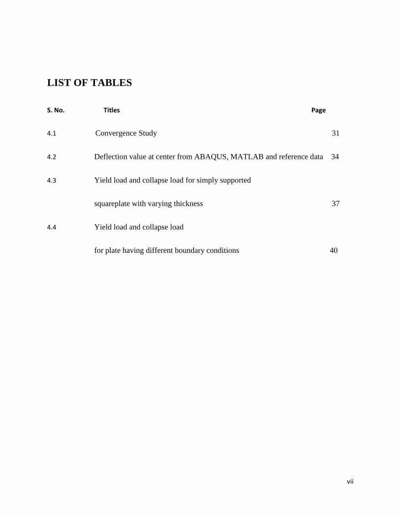
LIST OF TABLES

S. No. Titles Page

4.1 Convergence Study 31

4.2 Deflection value at center from ABAQUS, MATLAB and reference data 34

4.3 Yield load and collapse load for simply supported

squareplate with varying thickness 37

4.4 Yield load and collapse load

for plate having different boundary conditions 40

viii

LIST OF FIGURES

S. No. Titles Page

3.1 Linear and nonlinear spring characteristics 3

3.2 Large deflection of cantilever beam 4

3.3 Yield surface for isotropic strain-hardening material 6

3.5 Yield surface for kinematic strain-hardening material 7

3.6 Strain hardening softening curve for strain material 7

3.7 Flow chat of ABAQUS modeling and analysis steps 15

3.8 Eight-noded serendipity element 18

3.9 Warping in plate section 19

3.10 Elasto-plastic strain hardening behavior for the uniaxial case 27

4.1 Load diagram and plan view of plate 31

4.2 Convergence curve for different mesh size 32

4.3 Constitutive Relation for Perfectly plastic material 33

4.3 Stress flow pattern for plate having perfectly plastic properties 34

4.4 Load vs deflection curve for plate of 0.01m thickness in

ABAQUS and MATLAB 34

4.5 Stress flow pattern for plate having perfectly plastic properties 35

4.6 Load vs deflection curve for plate of 0.02m thickness in

ix

ABAQUS and MATLAB 38

4.7 Load vs deflection curve for plate of 0.03m thickness in

ABAQUS and MATLAB 39

4.8 Comparison curve between load and deflection of plate

of varying thickness in ABAQUS and MATLAB 39

4.9 Stress flow on plate having two opposite sides simply

supported and other two sides free 40

4.10 Stress flow on plate having two opposite sides fixed and other

two sides free 41

4.11 Stress flow on plate having three sides fixed and other side free 41

4.12 Stress flow on plate having all sides simply supported 42

4.13 Stress flow on plate having all sides fixed 42

4.14 Comparison curve between load and deflection values

for different boundary conditions 43

4.15 Constitutive Relation for Strain hardening material 44

4.16 Stress flow pattern for plate having strain hardening property

(ABAQUS) 45

4.17 Stress flow in strain hardening material from MATLAB 46

4.18 Load vs deflection curves for perfectly plastic and Strain hardening materials 47

x

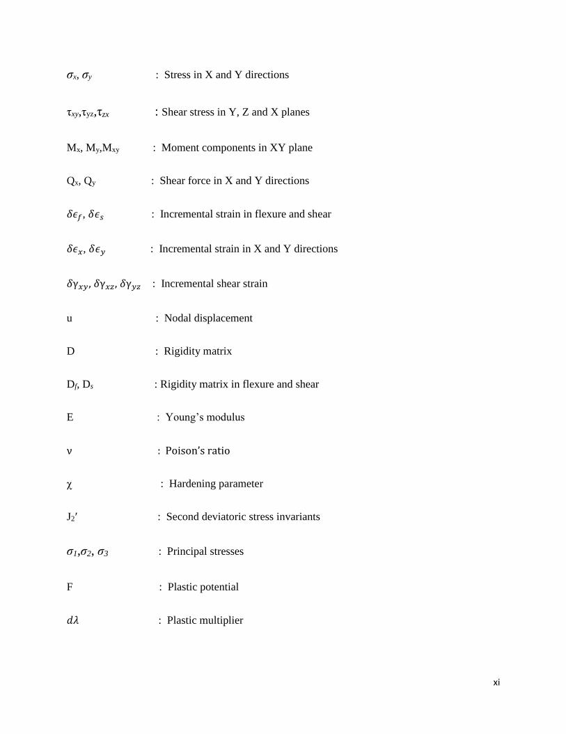
LIST OF ABBREVIATIONS

a,b : Length and width of plate

t : Thickness of plate

[K] : Stiffness matrix

[P] : Applied load vector

[d] : Deflection vector

[δ] : Vector of unkown

ψ (δ) : Residual load vector

ξ-η : Natural co-ordinates

𝑥𝑖 , 𝑦𝑖 : Co-ordinates of ith node

N : Shape functions

θx, θy : Rotation in X and Y direction

ϕx, ϕy : Shear deformation in X and Y direction

w : Deflection in Z direction

𝜖 : Total Strain

σ : Stress

𝜖𝑓 , 𝜖𝑠 : Strain in flexure and shear respectively

𝜖𝑥, 𝜖𝑦 : Strain in X and Y direction

ϒ𝑥𝑦,ϒ𝑥𝑧,ϒ𝑦𝑧 : Components of shear strain

σf, σs : Stress in flexure and shear plane

xi

σx, σy : Stress in X and Y directions

τxy,τyz,τzx : Shear stress in Y, Z and X planes

Mx, My,Mxy : Moment components in XY plane

Qx, Qy : Shear force in X and Y directions

𝛿𝜖𝑓, 𝛿𝜖𝑠 : Incremental strain in flexure and shear

𝛿𝜖𝑥, 𝛿𝜖𝑦 : Incremental strain in X and Y directions

𝛿γ𝑥𝑦, 𝛿γ𝑥𝑧, 𝛿γ𝑦𝑧 : Incremental shear strain

u : Nodal displacement

D : Rigidity matrix

Df, Ds : Rigidity matrix in flexure and shear

E : Young’s modulus

ν : Poison’s ratio

χ : Hardening parameter

J2′ : Second deviatoric stress invariants

σ1,σ2, σ3 : Principal stresses

F : Plastic potential

𝑑𝜆 : Plastic multiplier

1

CHAPTER 1

INTRODUCTION

2

Chapter 1

1. Introduction

Plates and shells are very important parts of several engineering structures. Analysis and design

of these origins are therefore always of interest to the scientific and engineering community.

Accurate and conventional valuations of the maximum load the structure can carry, along with

the equilibrium path followed in elastic and inelastic range are of paramount importance to

understand realistic behavior of structures.

Elastic behavior of plates and shells have been very closely studied, mostly by using of the finite

element method. On the other hand inelastic analysis, especially dealing with material

nonlinearity, has received just handful attention from the researchers. The elasto-plastic behavior

of structural elements are modelled using mathematical theory of plasticity and this includes

analysis of flow of plastic deformations in the regions where the yield criteria is fulfilled.

For nonlinear analysis many commercial software’s are available, such as ANSYS, ABAQUS,

etc. All these software’s are not tailor made applications which can work automatically on just

feeding simple input data. An acceptable analysis of any structure by using these commercial

software, and its correctness totally depends on the input values, especially when the material

properties used.

3

1.1 Non-Linearity

Non-linear structural problems include the variation of stiffness of the structure with the change

in deformation and the materials stress-strain behavior. Generally all physical structures exhibit

non-linear behavior. Linear analysis is a convenient approximation that is often adequate for

design purposes. It is obviously inadequate for many structural simulations including

manufacturing processes, such as forging or stamping; crash analyses; and analyses of rubber

components, such as tires or engine mounts. Since response of the structure to an external

applied load is not linear, the load versus deflection curve will not be linear. The force and

displacement relation for a spring with non-linear stiffening response is shown below.

Figure 1: linear and nonlinear spring characteristics

As response nonlinear system is not linear function of magnitude of applied load, the stiffness

cannot be directly calculated merely dividing load with deflection. Also it is not possible to

create solutions for different load cases by superposition.

4

Types of Nonlinearity:

Before discussing the numerical methods, the sources of nonlinearity have been penned below.

There are three types of nonlinearities.

1. Geometric nonlinearity

2. Material nonlinearity

3. Boundary nonlinearity

Geometric Nonlinearity:

This type of nonlinearity arises when large deflection affects the response of the structure.

Figure 1.2: Large deflection of cantilever beam

Geometric nonlinearity can be three types:

a) Large displacement and small strain behavior: this deal with the smallness of one of

the global coordinates of a body subjected to load.

b) Large displacement and large strain behavior: when changes to all the global

coordinates of the body are comparable, the stress distribution in any direction cannot

be neglected.

c) Linear stability analysis: if due to external load the body is on the verge of stable

equilibrium and any further load will cause an unstable equilibrium in the system, the

behavior of system can be considered as a linear function of applied load.

5

Material nonlinearity:

Material nonlinearity is caused due to the nonlinear relationship between stress and strain beyond

the elastic limit. Beyond this limit some portion of the member will start yielding and based on

materials, nonlinear constitutive relation start to respond in-elastically. This causes changes in

the stiffness of the member which depends on the material behavior called Elasto-plastic

behavior.

The present work involved only elasto-plastic behavior. An increase of the yield stress is referred

to as hardening and its decrease is called softening. Typically, many materials initially harden

and later soften as shown in Fig.1.4. A plot of a stress - strain curve defines material behavior.

Stress Hardening

Yield point softrning

E

Elastic

O Strain

Figure 1.3: Strain Hardening behavior

Based on stress-strain diagram material behavior can be classified as

1. Perfectly Plastic

2. Elasto-plastic Strain Hardening

3. Elasto-plastic Strain softening

6

1. Perfectly plastic: It is the property of material for which the stress, strain curve of the material

becomes parallel to strain axis, i.e. there is a large increase in strain for invariable yield stress

value.

Stress

Perfectly plastic

σy

E

Strain

Figure 1.4: Perfectly plastic behavior

2. Elasto-plastic strain hardening: Materials exhibit a characteristic called work or strain

hardening, which is strengthening of metal by plastic deformation. The yield surface for such

materials will in general increase in size with further straining. It can also be classified into two

types.

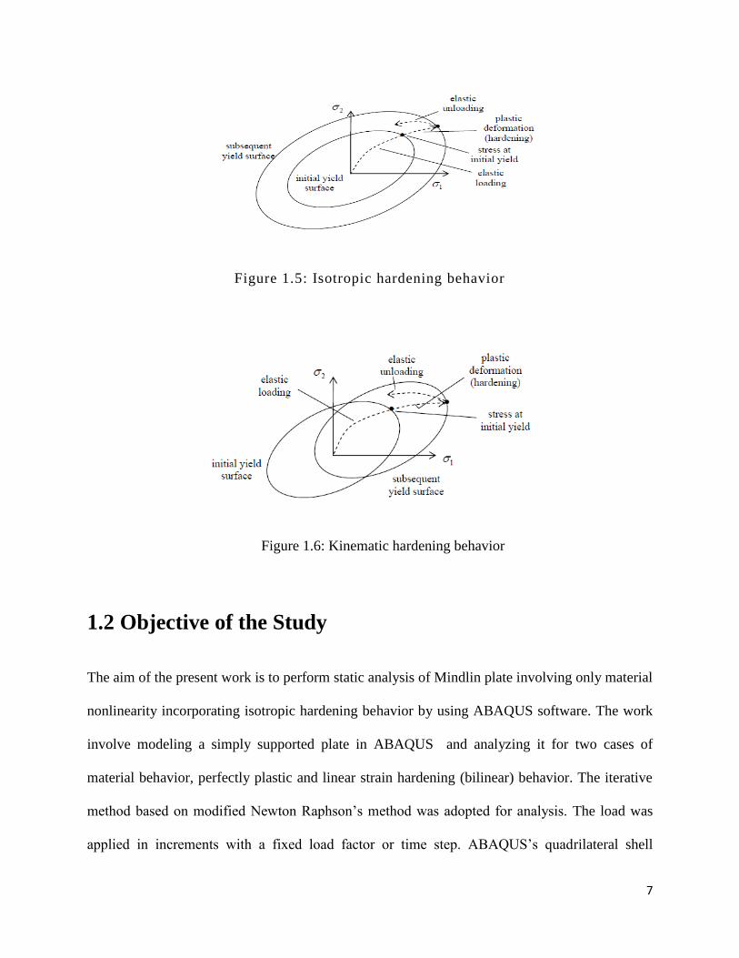
(i) Isotropic hardening (ii) Kinematic hardening

Isotropic hardening: It is characterized by the expanding yield surface of same shape with

increasing stress (ref.Fig.1.5).

Kinematic Hardening: It is characterized by the yield surface of same shape and size translating

in stress space (ref.Fig.1.6).

7

Figure 1.5: Isotropic hardening behavior

Figure 1.6: Kinematic hardening behavior

1.2 Objective of the Study

The aim of the present work is to perform static analysis of Mindlin plate involving only material

nonlinearity incorporating isotropic hardening behavior by using ABAQUS software. The work

involve modeling a simply supported plate in ABAQUS and analyzing it for two cases of

material behavior, perfectly plastic and linear strain hardening (bilinear) behavior. The iterative

method based on modified Newton Raphson’s method was adopted for analysis. The load was

applied in increments with a fixed load factor or time step. ABAQUS’s quadrilateral shell

8

element S8R was adopted with through the thickness stress integration (three point integration)

points and Von Mises yield criteria. The effect of thickness and different boundary conditions on

load carrying capacity, load deflection and spread or flows of plastic deformations are studied.

The ABAQUS results were compared with reference solutions by Owen and Hinton (1980) and

compared with results obtained from FEM based numerical analysis.

9

CHAPTER 2

REVIEW OF LITERATURE

10

Chapter 2

2. Literature review

The Reissiner-Mindlin plate theory is commonly used to analyze the bending behavior of elastic

plate subjected to transverse force.

Owen D. R. J. and Hinton E. (1980), this book has presented and demonstrated the use of finite

element based method for solution of problems involving plasticity. The detailed theory and

algorithm in the form of modular coding written in FORTRAN is also given. Problems related to

linear and nonlinear response of Mindlin and Kirchoff plates have been elaborately studied.

Talja A. and Pekka S. (1992) performed nonlinear analysis of two different cold formed high

strength steel (HSS) beams, shorter one for were studied for bending resistance across the cross-

section and longer beam for the lateral buckling. Both material and geometric nonlinearities

were studied using FEM analysis. They used shell elements to model the beams. Strength

calculation of beams showed that materials modeled with no imperfection can have 12 percent of

accuracy in strength prediction.

Hui Shen Shen (2000) performed a nonlinear analysis for a simply supported rectangular

moderately thick plate subjected to transverse central load resting on elastic supports. He

considered first order shear deformation effect and the formulas were based on Reissner-Mindlin

plate theory. Various numerical examples are solved and the performance of thick plate

influenced by various factors like foundation stiffness, plate loaded area, aspect ratio of plate,

transverse shear deformation has been analyzed.

11

WoelkePawel (2005) has presented a computational model for finite element, damaging and

elasto-plastic analysis of homogeneous and isotropic shell. Considering the non-layered

approach and updated Lagrangian method are used to describe the small strain geometric non-

linearity. Though multi layered approach in composite shell gives more accurate results, in

isotropic homogenous shells this becomes more complex, hence non layered approach is more

realistic.

Szwaja Nicolas (2012) has performed elastic and elasto-plastic analysis of plates subjected to

several boundary conditions and load using FEA ABAQUS. Here it can be concluded that by

placing different conditions on a simple geometry like cavity and pores analysis, it is simpler to

understand how FEA ABAQUS analyzes these models and how the strength of structure is

related to changing conditions.

Fallah N. et al. (2014) developed a finite volume based analysis to study the elastoplastic

bending behavior of plates. They applied Reissiner-Mindlin plate theory, performing layer-wise

approach and two iteration methods. Their results of studies are compared with available

reference from which it can be concluded that the developed finite volume based analysis has

significant capabilities for solid mechanics analysis.

12

CHAPTER 3

THEORY AND FORMULATION

13

Chapter 3

3. Theory and formulation

3.1ABAQUS Modeling and analysis

In ABAQUS modeling and analysis include following three steps:

1. Preprocessing

2. Simulation

3. Postprocessing

3.1.1 Preprocessing

It is the initial step to analyze the physical problem. In this step model of the physical problem is

defined and a ABAQUS input file (job.inp) in generated. Basic key points like material

properties, element type, boundary condition, load, contact, mesh are defined here.

3.1.2 Simulation

The simulation is normally run as a background process. In this step already generated ABAQUS

input file solves the numerical problem defined in the model. For example, output from a stress

analysis, problem includes displacement and stress values and are stored in binary files in

14

simulation which are further to be used in postprocessing. The output file is generated as job.

odb.

During simulation ABAQUS uses Newton Raphson method to solve the non-linear type

problems. Unlike linear analysis, load application to the system is incremental in non-linear case.

ABAQUS breaks the simulation stage into number of load increments and at the end of each

load increment it finds an approximate equilibrium configuration. Sometimes ABAQUS takes a

number of iterations to find an acceptable solution depends on tolerance specified, for a

particular load increment. Finally the cumulative summation of all load incremental responses is

the approximate solution to that non-linear problem. This way ABAQUS uses both incremental

and iterative methods to solve non-linear problems. There are three phases in simulation stage

Analysis step

Load increment

Iteration

Analysis step which generally consists of loading option, output request. Output request

describes the values of required parameters like displacement, stress, strain, reaction force,

bending moment etc.

In increment step, first load increment is to be defined by the user and the subsequent increments

will be chosen by ABAQUS automatically.

Iteration continues till ABAQUS optimize the residual forces to the given tolerance value.Hence,

after each load increment the structure satisfies the equilibrium conditions and corresponding

output request values are to be written to the output database file.

15

3.1.3 Postprocessing

Once the simulation is over, the calculated variables like stresses, displacements, strain, reaction

forces etc. can be displayed through Visualization module of ABAQUS. The visualization

module has a variety of options to display the results such as animation, color contour plots,

deformed shape plots and X-Y plots.

In our work, it is required to find out deflections, plastic strain, stresses and yield stress values at

specified nodes. All these values can be obtained from the visualization module of ABAQUS.

Figure 3.1: Flow-chat of ABAQUS modeling and analysis

16

3.2.3 Element Type

The correct choice of element for a particular simulation is very important to meet the desired

accuracy in the result. The ABAQUS/Standard solid element can be classified into two

categories.

a) First order (linear) interpolation element

b) Second order (quadratic) interpolation element

The first order element type is used for the two dimensional analysis and second order element

type is used for three dimensional analysis. While selecting element, ABAQUS gives a number

of choices like linear, quadratic, brick etc. In the present study 8 noded quadratic shell element

S8R is adopted where R represents reduced integration type, S stands for shell element having 8

nodes in which each node is assigned with 6 degrees of freedom. The present study involves very

large mesh distortions and large strain analysis.

3.2 Formulation for Finite Element Method

3.3.1 Equilibrium equations

[K] δ + P = ψ(δ) ≠ 0 (1)

Where [K] is assembled stiffness matrix

P is vector of applied load

δ is vector of basic unknown i.e. defections d

ψ(δ) is vector of residual force.

17

If the coefficients of the matrix K depend on the unknowns δ or their derivatives, the problem

clearly becomes nonlinear. In this case, direct solution of equation system (1) is generally

impossible and an iterative scheme must be adopted. For nonlinear situations, in which the

stiffness depends on the degree of displacement in some manner, K is equal to the local gradient

of the force-displacement relationship of the structure at any point and is termed the tangential

stiffness. The analysis of such problems must proceed in an incremental manner since the

solution at any stage may not only depend on the current displacements of the structure, but also

on the previous loading history. In present study Newton-Raphson technique following the

tangential stiffness method is adopted for nonlinear analysis of Mindlin plate.

3.3.2 Discretization:

The arbitrary shape of the whole plate is mapped into a Master Plate of square region [-1, +1] in

the ξ-η plane with the help of the relationship given by

x =∑ 𝑁𝑖(𝜉, 𝜂)𝑥𝑖8𝑖=1 (2)

y =∑ 𝑁𝑖(𝜉, 𝜂)𝑦𝑖8𝑖=1 (3)

where (𝑥𝑖,𝑦𝑖) are the coordinates of the 𝑖𝑡ℎ node on the boundary of the plate in the x-y plane and

𝑁𝑖 (𝜉, 𝜂) are the corresponding cubic Serendipity shape functions presented below.

18

8-noded Serendipity element

N1 = 1 4⁄ (η – 1) (1- ξ) (η + ξ + 1)

N2 = 1 2⁄ (1 - η) (1- ξ 2)

N3 = 1 4⁄ (η – 1) (1- ξ) (η - ξ + 1)

N4 = 1 2⁄ (1 - η2) (1 + ξ)

N5 = 1 4⁄ (1 + η) (1 + ξ) (η + ξ - 1)

N6 = 1 2⁄ (1 + η) (1- ξ 2)

N7 = 1 4⁄ (1 + η) (1 – ξ) (η - ξ - 1)

N8 = 1 2⁄ (1 - η2) (1 - ξ)

[N] = [N1 N2 N3 N4 N5 N6 N7 N8] (4)

19

3.3.3 Plate element formulation:

The displacement field at any point within the element is given by

{𝑈} = [

𝑢 − 𝑧 θₓ(x, y)

𝑢 − z θy(x, y)w(x, y)

] (5)

Owing to the shear deformations, certain warping in the section occurs as shown in Fig. 3.3.

However, considering the rotations θx and θy as the average and linear variation along the

thickness of the plate, the angles ϕx and ϕy denoting the average shear deformation in and x-y

Figure 3.3: warping in plate section

{𝛳𝑥𝛳𝑦} = {

𝜕𝑤

𝜕𝑥+ 𝜑𝑥

𝜕𝑤

𝜕𝑦+ 𝜑𝑦

} (6)

20

The plate strains are described in terms of middle surface displacements i. e. x-y plane coincides

with the middle surface .The strain matrix is given by

{𝜖} = {𝜖𝑓𝜖𝑠} =

{

𝜖𝑥𝜖𝑦ϒ𝑥𝑦ϒ𝑥𝑧ϒ𝑦𝑧}

(7)

And stress matrix is given by

{𝜎} = {𝜎𝑓𝜎𝑠} =

{

𝜎𝑥𝜎𝑦τ𝑥𝑦τ𝑥𝑧τ𝑦𝑧}

(8)

For non-layer approach

We interpret

[𝜎𝑓] = [ 𝑀𝑥 𝑀𝑦 𝑀𝑥𝑦]T (9)

and [𝜎𝑠 = [ 𝑄𝑥 𝑄𝑦]T (10)

Since iterative method is used for analysis, the corresponding relations in incremental form can

be written as

{𝛿𝜖} = {𝛿𝜖𝑓𝛿𝜖𝑠

} =

{

𝛿𝜖𝑥𝛿𝜖𝑦𝛿γ𝑥𝑦𝛿γ𝑥𝑧𝛿γ𝑦𝑧}

(11)

21

𝛿𝜖𝑓 = 𝑧 [−𝜕𝛿𝛳𝑥

𝜕𝑥−𝜕𝛿𝛳𝑦

𝜕𝑦−(

𝜕𝛿𝛳𝑦

𝜕𝑥+𝜕𝛿𝛳𝑥

𝜕𝑦)]T (12)

𝛿𝜖𝑠 = [𝜕𝛿𝑤

𝜕𝑥− 𝛿𝛳𝑥,

𝜕𝛿𝑤

𝜕𝑦− 𝛿𝛳𝑦]

T (13)

3.3.4 Strain displacement relationship:

For an isotropic material the displacement can be written as

U=∑ 𝑁𝑖(𝜉, 𝜂)𝑢𝑖8𝑖=1 (14)

Where ui is nodal displacement vector at ith node may be represented as

ui = [wi, 𝛳𝑥𝑖, 𝛳𝑦𝑖]T (15)

U = [w, 𝛳𝑥, 𝛳𝑦]T (16)

The flexural strain –displacement equation in incremental form is given as

𝛿𝜖𝑓 =∑ 𝐵𝑓𝑖𝛿𝑢𝑖8𝑖=1 (17)

Where 𝐵𝑓𝑖 =

[ 0 −

𝜕𝑁𝑖

𝜕𝑥0

0 0 −𝜕𝑁𝑖

𝜕𝑦

0 −𝜕𝑁𝑖

𝜕𝑦−𝜕𝑁𝑖

𝜕𝑥

]

(18)

The incremental shear strain displacement equation is

𝛿𝜖𝑠 =∑ 𝐵𝑠𝑖𝛿𝑢𝑖8𝑖=1 (19)

22

Where 𝐵𝑠𝑖 = [

𝜕𝑁𝑖

𝜕𝑥−𝑁𝑖 0

𝜕𝑁𝑖

𝜕𝑦0 −𝑁𝑖

] (20)

3.3.5 Virtual work Equation

Giving a virtual displacement 𝛿𝑢 to the system the virtual work statement may be written as

∑ [𝛿𝑢𝑖]𝑇 {∫𝐴 ∫ [𝐵𝑓𝑖]

𝑇𝜎′𝑓𝑧 + [𝐵𝑠𝑖]

𝑇𝜎𝑠′𝑧 − [𝑁𝑖]𝑇𝑞

𝑡/2

−𝑡/2} 𝑑𝑧 𝑑𝐴𝑛

𝑖=1 = 0 (21)

or ∑ ψi(u) = 0𝑛𝑖=1

where ψi is residual force vector at ith node.

Since equation (21) must be true for any set of virtual displacements we get (for layered model)

{∫ 𝐴 ∫ [𝐵𝑓𝑖]𝑇𝜎′𝑓𝑧 + [𝐵𝑠𝑖]

𝑇𝜎′𝑠𝑧 − [𝑁𝑖]𝑇𝑞

𝑡/2

−𝑡/2} 𝑑𝑧 𝑑𝐴 = 0 (22)

For nonlayer model

∫ [[𝐵𝑓𝑖]𝑇𝜎𝑓 + [𝐵𝑠𝑖]

𝑇𝜎𝑠 − [𝑁𝑖]𝑇𝑞] 𝑑𝐴 = 0

𝐴(23)

ψ= [ψ1, ψ2,ψ3,………ψn]T (24)

Contribution to residual force vector is evaluated at element level and then assembled to for

residual force vector ψ.

23

3.3.5Formulation in inelastic region

In this study material non linearity due to an elasto-plastic material response is considered and

isotropic effects are included in the yielding behavior. To model elasto-plastic material behavior

in inelastic region two conditions have to be met:

1. A yield criterion representing the stress level at which plastic flow commences must be

postulated,

2. A relationship between stress and strain must be developed for post yielding behavior.

Before onset of yielding the relationship between stress and strain is given by

σ = D*ε (25)

D is rigidity matrix

𝐷 = [𝐷𝑓𝐷𝑠] (26)

𝐷𝑓 =𝐸𝑡3

12(1 − 𝜈2)[

1 𝜈 0𝜈 1 0

0 0(1 − 𝜈)

2

]

𝐷𝑠 =𝐸𝑡

2.4(1+𝜈)[1 00 1

] (28)

For the isotropic material the yield criteria adopted is a generalization of the Von Mises law.

24

The Von Mises Yield Criterion:

In general form yield criterion is written as

F (σ, χ) = f (σ) –Y (χ) = 0 (29)

wherefis some function of the deviatoric stress invariants and Y is yield level which is function

of hardening parameter χ.

Defining the effective stress σ for isotropic Von Mises material as

σ = √3𝑘 (30)

where 𝑘 = (J2′)1/2 (31)

and J2′ is the second deviatoric stress invariants

J2′= 1

6 [(σ1 – σ2)

2 + [(σ2 – σ3)2 + [(σ3 – σ1)

2]

where σ1,σ2,σ3 are principal stresses

= 1

2 [σx’

2 + σy’2 + σz’

2 ] + τxy2 + τyz

2 + τzx2 (33)

3.3.6 Elasto-plastic stress strain relation

After initial yielding the material behavior will be partly elastic and partly plastic. During any

increment of stress, the changes of strain are assumed to be divisible into elastic and plastic

components, so that

dε = dεe + dεp (34)

25

The elastic strain increment is given by the incremental form of

dεe = [D]-1dσ (35)

and the plastic strain increment by the flow rule

dεp = 𝑑𝜆𝜕𝑄

𝜕χ (36)

where Q is defined as plastic potential and 𝑑𝜆 is a proportional constant called plastic multiplier.

The assumption Q ≡ fgives rise to an associated plasticity theory, in which case equation (36)

represents the normality condition; since 𝜕𝑓

𝜕σ is a vector directed normal to the yield surface in a

stress space geometrical interpretation.

The differential form of eq. (29) is

dF =𝜕𝐹

𝜕σdσ +

𝜕𝐹

𝜕χdχ = 0 (37)

or aTdσ – Adλ = 0 (38)

in which the flow vector aT is define as

aT = 𝜕𝐹

𝜕σ = [

𝜕𝐹

𝜕σx ,𝜕𝐹

𝜕σy ,

𝜕𝐹

𝜕τxy ,

𝜕𝐹

𝜕τyz ,

𝜕𝐹

𝜕τzx] (39)

26

Equation (37) & (38) can be reduced to get

A = -1

𝑑𝜆

𝜕𝐹

𝜕χdχ (40)

Total incremental strain is

dε = [D]-1dσ + 𝑑𝜆 𝜕𝐹

𝜕χ (41)

Pre-multiplying both sides by aT D and eliminating aTdσ by using eq. (40), we get 𝑑𝜆 to be

𝑑𝜆 = 1

[𝐴+aT 𝐷 a]aT DT a dε (42)

Manipulation of equation (34) to equation (42) will give elasto-plastic incremental stress strain

relationship

Dσ= Depdε (43)

Where Dep = 𝐷 −𝐷 a aT D

[𝐴+aT 𝐷 a] (44)

The hardening parameter A can be deduced from uniaxial conditions as

A = H′ = 𝜕𝜎

𝜕𝜖𝑝 (45)

Thus A is obtained to be the local slope of the uniaxial stress/plastic strain curve and can be

determined experimentally from Fig.

27

Fig. 3.4: Elasto-plastic strain hardening behavior for the uniaxial case

A= H′ = 𝐸𝑇

1− 𝐸𝑇

𝐸⁄ (46)

The incremental stress-strain resultant relationship is given as

[𝑑𝜎𝑓𝑑𝜎𝑠

] = [(𝐷𝑒𝑝)𝑓 0

0 𝐷𝑠] [𝑑휀𝑓𝑑휀𝑠

] (47)

For Mindlin plate, yield function F is assumed to be function of 𝜎𝑓, the direct stresses associated

with flexure only hence 𝐷𝑠 always remain elastic.

3.3.7 Tangential Stiffness matrix:

From equation (22),the tangential stiffness matrix can be written as

𝐾𝑇 = ∫ [[𝐵𝑓]𝑇(𝐷𝑒𝑝)𝑓 𝐵𝑓 +

[𝐵𝑠]𝑇𝐷𝑠𝐵𝑠] 𝑑𝐴𝐴

(48)

28

CHAPTER 4

RESULT AND DISCUSSION

29

4.1 Methodology

1. A convergence study was performed to fix the mesh size for analysis in ABAQUS.

2. To check the accuracy of element selected, time step, analysis method elastic analysis

was performed using ABAQUS and results were compared with exact solution.

3. The plate was analysed considering perfectly plastic material behaviour. The results

were validated with reference solutions by Owen and Hinton (1980).The results were

also compared with results obtained from FEM based numerical solutions.

4. The effect of thickness and boundary conditions were studied.

5. The plate was analysed considering strain hardening material behaviour. The results

were validated with numerically solved results.

4.2 Convergence study

The convergence study is carried out to determine the mesh size or the number of elements

required for the Finite Element Analysis. A plate having all sides simply supported is subjected

to a uniformly distributed load of magnitude 1 kN/m2.

Figure 4.1: Load diagram and plan view of plate

30

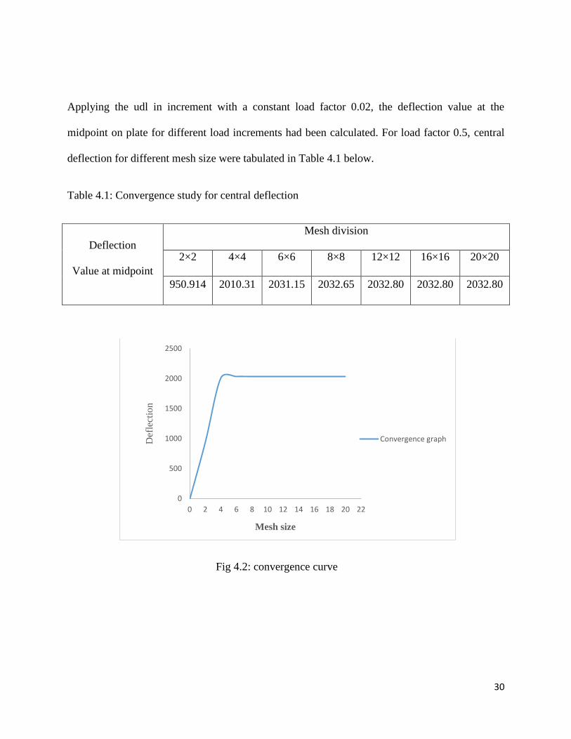
Applying the udl in increment with a constant load factor 0.02, the deflection value at the

midpoint on plate for different load increments had been calculated. For load factor 0.5, central

deflection for different mesh size were tabulated in Table 4.1 below.

Table 4.1: Convergence study for central deflection

Deflection

Value at midpoint

Mesh division

2×2 4×4 6×6 8×8 12×12 16×16 20×20

950.914 2010.31 2031.15 2032.65 2032.80 2032.80 2032.80

Fig 4.2: convergence curve

0

500

1000

1500

2000

2500

0 2 4 6 8 10 12 14 16 18 20 22

Def

lect

ion

Mesh size

Convergence graph

31

From the above table it can be concluded that the deflection value after taking mesh size (12×12)

and onwards does not vary much i.e. results show good convergence for mesh division (12×12).

Hence 12x12 mesh division is used for further study.

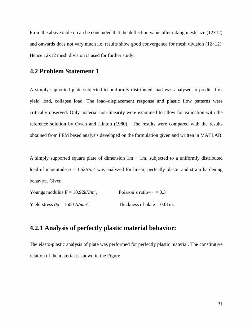
4.2 Problem Statement 1

A simply supported plate subjected to uniformly distributed load was analysed to predict first

yield load, collapse load. The load–displacement response and plastic flow patterns were

critically observed. Only material non-linearity were examined to allow for validation with the

reference solution by Owen and Hinton (1980). The results were compared with the results

obtained from FEM based analysis developed on the formulation given and written in MATLAB.

A simply supported square plate of dimension 1m × 1m, subjected to a uniformly distributed

load of magnitude q = 1.5kN/m2 was analyzed for linear, perfectly plastic and strain hardening

behavior. Given

Youngs modulus E = 10.92kN/m2, Poisson’s ratio= ν = 0.3

Yield stress σ0 = 1600 N/mm2. Thickness of plate = 0.01m.

4.2.1 Analysis of perfectly plastic material behavior:

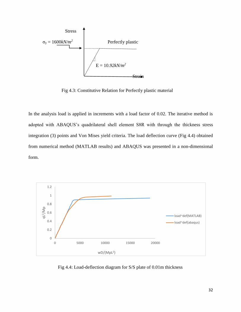
The elasto-plastic analysis of plate was performed for perfectly plastic material. The constitutive

relation of the material is shown in the Figure.

32

Stress

σy = 1600kN/m2 Perfectly plastic

E = 10.92kN/m2

Strain

Fig 4.3: Constitutive Relation for Perfectly plastic material

In the analysis load is applied in increments with a load factor of 0.02. The iterative method is

adopted with ABAQUS’s quadrilateral shell element S8R with through the thickness stress

integration (3) points and Von Mises yield criteria. The load deflection curve (Fig 4.4) obtained

from numerical method (MATLAB results) and ABAQUS was presented in a non-dimensional

form.

Fig 4.4: Load-deflection diagram for S/S plate of 0.01m thickness

0

0.2

0.4

0.6

0.8

1

1.2

0 5000 10000 15000 20000

qL2 /

Mp

wD/(MpL2)

load~def(MATLAB)

load~def(abaqus)

33

From the graph the maximum deflection occurs at load 0.99kN/m2 in ABAQUS and0.94kN/m2 in

MATLAB. The first yield occurs at load 0.81kN/m2 and the collapse load is 0.99kN/m2.

Comparison with reference data:

Central deflection is compared at load factor 0.856. ABAQUS result is compared with reference

data by Owen and numerical result from MATLAB coding. Nonlinearity for transverse shear is

not considered in FEM modeling by Owen and the analysis adopted is non-layered approach

whereas ABAQUS considered nonlinearity for flexure and transverse shear both. Hence there is

difference in results. That shows the effect of residual transverse shear.

Table 4.2: Deflection value at center from ABAQUS, MATLAB and reference data

Present study

(from ABAQUS)

Numerical result

(from MATLAB)

Reference Value

(from Owen and Hinton)

3739.923×10-3 3494.82×10-3 3496.31×10-3

Plastic Flow pattern:

The main objective of the present work is to track the progressive plasticization of the cross

sections. Since the stresses are calculated at different load steps, yielding of sections can be

easily tracked which give an idea of plastic flow in the plate. The Figures give an idea of plastic

flow in simply supported plate. The side by side figures represent stress contours obtained at

different stages of loadings, from ABAQUS software and MATLAB coding.

34

ABAQUS MATLAB

Stress Contour for load q=0.15kN/m2 (L.F. =5)

q = 0.45kN/m2 (L.F. =15)

q = 0.48kN/m2(L.F. =16)

35

q = 0.60kN/m2 (L.F. =20)

q = 0.75kN/m2(L.F. =25)

q = 0.99kN/m2 (L.F. =33) (q = 0.94kN/m2)

Fig 4.5: stress flow pattern for plate having perfectly plastic properties

36

The plastic flow followed the yield line pattern for s/s slab. The initial yielding started at corner

points and further spread justifying the well-known corner lever effect in a simply supported two

way slab used in yield analysis of slab. This causes lifting of corners. Both analysis exhibited

same phenomenon and same pattern of plastic flow. A comparison for yield and collapse loads

are given in Table.

Effect of thickness:

The FEM formulation did not include non-linearity in transverse shear while ABAQUS analysis

takes care of it. Hence to observe the effect of thickness on elasto-plastic behavior of simply

supported plate further analysis were carried out by taking thickness as 0.02 and 0.03. This

would gave an idea about the influence of the transverse shear on elasto-plastic behavior of plate.

For 0.01m thickness this influence is very small. The effect were observed in terms of load-

deflection curves, yield load and collapse load by using numerical method (MATLAB)and

ABAQUS. The curves are shown in Fig and Fig. and Table gives a comparison between yield

and collapse loads.

Table 4.3: Yield and collapse load for a square plate with different thickness

Thickness(m)

ABAQUS MATLAB

Load (kN/m2) at

first yield

Load (kN/m2) at

collapse

Load (kN/m2)

at first yield

Load (kN/m2)

at collapse

0.01 0.54 0.99 0.54 0.94

0.02 2.57 4.00 2.57 3.80

0.03 5.40 8.80 5.40 7.92

37

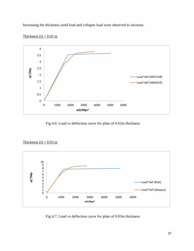
Increasing the thickness yield load and collapse load were observed to increase.

Thickness (t) = 0.02 m

Fig 4.6: Load vs deflection curve for plate of 0.02m thickness

Thickness (t) = 0.03 m

Fig 4.7: Load vs deflection curve for plate of 0.03m thickness

0

0.5

1

1.5

2

2.5

3

3.5

4

0 1000 2000 3000 4000 5000 6000

qL2 /

Mp

wD/MpL2

Load~def (MATLAB)

Load~def (ABAQUS)

0123456789

10

0 1000 2000 3000 4000 5000 6000

qL2 /

Mp

wD/MpL2

Load~def (Mat)

Load~Def (Abaqus)

38

A comparison graph between yield load and collapse load at different thickness obtained from

ABAQUS Software and MATLAB modeling is represented below.

Fig 4.8: Load vs deflection curves for plate of varying thickness

Since ABAQUS considers nonlinearity in flexure and transverse shear both, a higher deflection

value is observed as compared to numerical approach (MATLAB coding). Also the graph

concludes a larger variation in value with increased thickness value.

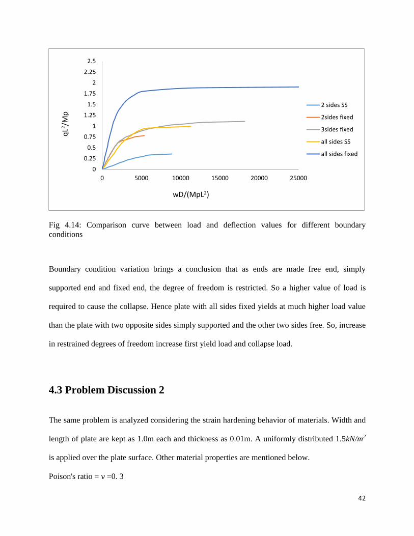
Effect of Boundary Conditions:

The plate of same dimensions was analyzed for different boundary conditions by ABAQUS

software. The variation were observed in terms of yield load, collapse load and plastic flow. The

comparison of yield and collapse loads is given in Table

0

1

2

3

4

5

6

7

8

9

10

0 5000 10000 15000 20000

qL2 /

Mp

wD/(MpL2)

t=0.03 (Abq)

t=0.02 (Abq)

t=0.01

t=0.03 (Matlab)

t=0.02 (Matlab)

t=0.01 (Matlab)

39

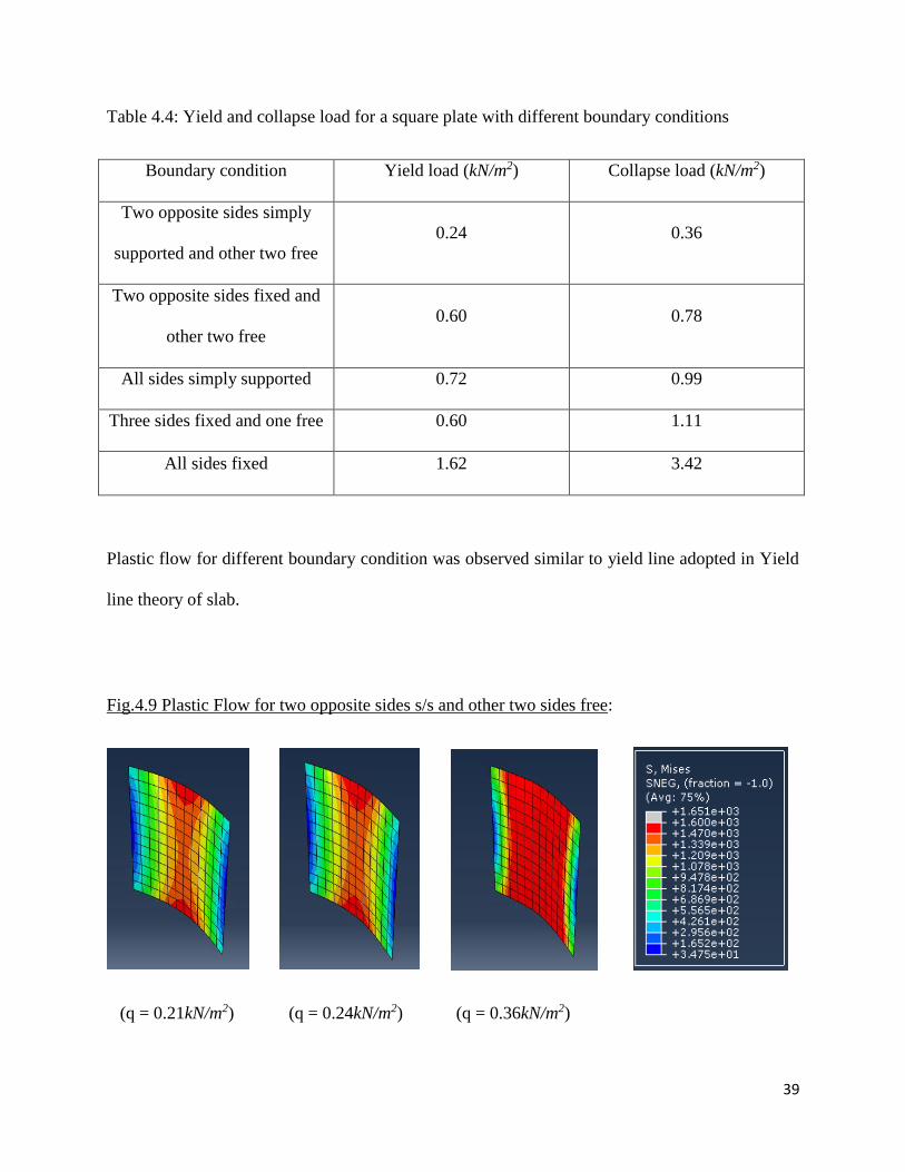
Table 4.4: Yield and collapse load for a square plate with different boundary conditions

Boundary condition Yield load (kN/m2) Collapse load (kN/m2)

Two opposite sides simply

supported and other two free

0.24 0.36

Two opposite sides fixed and

other two free

0.60 0.78

All sides simply supported 0.72 0.99

Three sides fixed and one free 0.60 1.11

All sides fixed 1.62 3.42

Plastic flow for different boundary condition was observed similar to yield line adopted in Yield

line theory of slab.

Fig.4.9 Plastic Flow for two opposite sides s/s and other two sides free:

(q = 0.21kN/m2) (q = 0.24kN/m2) (q = 0.36kN/m2)

40

Figure 4.10 Plastic Flow for Two opposite sides fixed and other two free:

(q = 0.30kN/m2) (q = 0.60kN/m2) (q = 0.78kN/m2)

Figure 4.11 Plastic Flow for Three sides fixed supported:

(q = 0.75kN/m2) (q = 0.93kN/m2) (q = 1.11kN/m2)

41

Figure 4.12: Plastic Flow for All sides simply supported:

(q = 0.51kN/m2) (q = 0.69kN/m2) (q = 0.99kN/m2)

Figure 4.13: Plastic Flow for All sides fixed support:

(q = 0.5kN/m2) (q = 1.5kN/m2) (q = 3.32kN/m2)

42

Fig 4.14: Comparison curve between load and deflection values for different boundary

conditions

Boundary condition variation brings a conclusion that as ends are made free end, simply

supported end and fixed end, the degree of freedom is restricted. So a higher value of load is

required to cause the collapse. Hence plate with all sides fixed yields at much higher load value

than the plate with two opposite sides simply supported and the other two sides free. So, increase

in restrained degrees of freedom increase first yield load and collapse load.

4.3 Problem Discussion 2

The same problem is analyzed considering the strain hardening behavior of materials. Width and

length of plate are kept as 1.0m each and thickness as 0.01m. A uniformly distributed 1.5kN/m2

is applied over the plate surface. Other material properties are mentioned below.

Poison's ratio = ν =0. 3

0

0.25

0.5

0.75

1

1.25

1.5

1.75

2

2.25

2.5

0 5000 10000 15000 20000 25000

qL2

/Mp

wD/(MpL2)

2 sides SS

2sides fixed

3sides fixed

all sides SS

all sides fixed

43

Youngs modulus = E = 10.92 N/mm2

ET = E

2

Stress Strain hardening

σy ET

E

O Strain

Fig 4.15: Constitutive Relation for Strain hardening material

The main objective of the work is to track the progressive plasticization of the cross sections.

Since the stresses are calculated at different load steps, yielding of sections can be easily tracked

which give an idea of plastic flow in the plate. The figures give an idea of plastic flow in simply

supported plate. Due to strain hardening property, the plate will yield at a higher load. After

yielding there will be a change in slope of stress–strain curve, whose value is taken as half of

initial Youngs modulus value. Maximum deflection values at center of plate obtained from

ABAQUS software and MATLAB coding are compared in the following table.

Plastic flow pattern:

44

(q = 0.12kN/m2) (q = 0.25kN/m2) (q = o.45kN/m2)

(q = 0.75kN/m2) (q = 1.02kN/m2) (q = 1.11kN/m2)

Fig 4.16: Stress flow pattern for plate having strain hardening property (ABAQUS)

The plastic flow followed the yield line pattern for s/s slab. The initial yielding started at corner

points and further spread justifying the well-known corner lever effect in a simply supported two

way slab used in yield analysis of slab. The white shows that because of strain hardening

behavior of plate, the yield stress value exceeds the given yield value 1600kN/m2.

45

Fig 4.17: Stress flow in strain hardening material from MATLAB

A comparison curve between deflection values in plastic state and strain hardening state is

plotted infig.4.18.

Fig 4.18: Load vs deflection curves for perfectly plastic and Strain hardening materials

0

0.2

0.4

0.6

0.8

1

1.2

0 2000 4000 6000 8000 10000 12000

qL

2/M

p

wD/(MpL2)

Load~Def (Perfectly plastic)

Load~Def(Strain hardening)

46

From the figure it is clearly visible that up to elastic range both curves are identical, but beyond

yielding due to strain hardening property, the plate takes a higher load value and finally collapses

at 1.11kN/m2 and almost follow the loading path.

47

CHAPTER 5

CONCLUSION

48

Chapter 5

Conclusion

The conclusions drawn from the present study are

1. The results obtained from ABAQUS are higher than results obtained from FEM based

numerical method because it incorporate nonlinearity in flexure and shear both.

3. Lower yield loads and higher collapse loads are obtained from ABAQUS. Because a non-

layered approach is used in formulations of FEM modeling. So first yield is observed when

whole section has plasticized.

4. For plate thickness of 0.01m the influence of transverse shear on plastic behavior is small

represented by difference in ABAQUS values and numerical values.

5. The influence of shear is observed to increase with increase in plate thickness.

6. The yield loads and collapse loads are observed to increase with increase in restrained degrees

of freedom depending on the boundary conditions of plate.

7. Plastic flows are observed to follow the pattern as given by yield line theory for various

boundary conditions.

8. The plastic flow pattern for strain hardening material clearly represents the isotropic strain

hardening flow where the subsequent yield surfaces are a uniform expansion of the original yield

curve. These are clearly visualized through the stress contour plots drawn in different stages of

loadings in both ABAQUS and numerical method.

49

In problems dealing material non-linearity, convergence is required to satisfy the equilibrium

condition and the stress conditions. Since analysis method follow step by step incremental

approach with repetitive computations, this may lead to the error accumulations. Therefore the

procedure is very sensitive and results depend on adopted incremental load (time step) and

tolerance value.

50

References

1. Owen D.R.J. and Hinton E. (1980): Finite element in plasticity: Theory and Practice,

Dept. of civil engineering, University College of Swansea, U.K., 121-152, 319-373.

2. Talja A. and Pekka S. (1992): bending strength of beams with nonlinear analysis,

Rakenteiden Mekaniikka, 25, 50-67.

3. Shen Shen Hui (2000): Nonlinear bending of simply supported rectangular Reissner–

Mindlin plates under the transverse and in-plane loads and resting on elastic

foundations, Engineering Structure, 22, 847-856.

4. PawelWoelke (2005): computational model for elasto-plastic and damage analysis of

plates and shells.

5. Szwaja Nicolas (2012): Elastic and Elasto-Plastic Finite Element Analysis of a tension

test specimen with and without voids, 15,147-175.

6. Fallah N. and Parayandeh A. (2014): A novel finite volume based formulation for the

elasto-plastic analysis of plates, Thin-walled Structure, 77,153-164

7. ABAQUS/CAE manual