170
ELEC 301 Projects Fall 2009 Collection Editor: Rice University ELEC 301

ELEC 301 Projects Fall 2009
Collection Editor:Rice University ELEC 301


ELEC 301 Projects Fall 2009
Collection Editor:Rice University ELEC 301
Authors:
Anthony AustinJeffrey Bridge
Robert BrockmanDan Calderon
Lei CaoGrant Cathcart
Sharon DuCatherine Elder
Jose GarciaGilberto Hernandez
Peter HokansonSeoyeon(Tara) Hong
Graham HouserChinwei HuAlysha JeansStephen Jong
James KohliStephen Kruzick
Kyle LiHaiying Lu
Stamatios MastrogiannisNicholas Newton
Norman PaiSam SoundarCynthia Sung
Matt SzalkowskiBrian VielYilong Yao
Jeff YehAron Yu
Graham de Wit
Online:< http://cnx.org/content/col11153/1.3/ >
C O N N E X I O N S
Rice University, Houston, Texas

This selection and arrangement of content as a collection is copyrighted by Rice University ELEC 301. It is licensed
under the Creative Commons Attribution 3.0 license (http://creativecommons.org/licenses/by/3.0/).
Collection structure revised: December 26, 2009
PDF generated: October 29, 2012
For copyright and attribution information for the modules contained in this collection, see p. 154.

Table of Contents
1 Digital Song Identi�cation Using Frequency Analysis
1.1 Introduction . . . . . . . . . . . . . . . . . . . . . . . . . . . . . . . . . . . . . . . . . . . . . . . . . . . . . . . . . . . . . . . . . . . . . . . . . . . . . . . . . 11.2 The Fingerprint of a Song . . . . . . . . . . . . . . . . . . . . . . . . . . . . . . . . . . . . . . . . . . . . . . . . . . . . . . . . . . . . . . . . . . . 11.3 The Fingerprint Finding Algorithm . . . . . . . . . . . . . . . . . . . . . . . . . . . . . . . . . . . . . . . . . . . . . . . . . . . . . . . . . . 21.4 The Resulting Fingerprint . . . . . . . . . . . . . . . . . . . . . . . . . . . . . . . . . . . . . . . . . . . . . . . . . . . . . . . . . . . . . . . . . . . 41.5 Matched Filter for Spectrogram Peaks . . . . . . . . . . . . . . . . . . . . . . . . . . . . . . . . . . . . . . . . . . . . . . . . . . . . . . . 61.6 The Matched Filter Algorithm . . . . . . . . . . . . . . . . . . . . . . . . . . . . . . . . . . . . . . . . . . . . . . . . . . . . . . . . . . . . . . . 61.7 Results . . . . . . . . . . . . . . . . . . . . . . . . . . . . . . . . . . . . . . . . . . . . . . . . . . . . . . . . . . . . . . . . . . . . . . . . . . . . . . . . . . . . . . 91.8 About the Team . . . . . . . . . . . . . . . . . . . . . . . . . . . . . . . . . . . . . . . . . . . . . . . . . . . . . . . . . . . . . . . . . . . . . . . . . . . . 12
2 A Matrix Completion Approach to Sensor Network Localization
2.1 Introduction . . . . . . . . . . . . . . . . . . . . . . . . . . . . . . . . . . . . . . . . . . . . . . . . . . . . . . . . . . . . . . . . . . . . . . . . . . . . . . . . 132.2 Matrix Completion: An Overview . . . . . . . . . . . . . . . . . . . . . . . . . . . . . . . . . . . . . . . . . . . . . . . . . . . . . . . . . . 132.3 Simulation Procedure . . . . . . . . . . . . . . . . . . . . . . . . . . . . . . . . . . . . . . . . . . . . . . . . . . . . . . . . . . . . . . . . . . . . . . . 142.4 Results, Conclusions, and Future Work . . . . . . . . . . . . . . . . . . . . . . . . . . . . . . . . . . . . . . . . . . . . . . . . . . . . . 162.5 Acknowledgments . . . . . . . . . . . . . . . . . . . . . . . . . . . . . . . . . . . . . . . . . . . . . . . . . . . . . . . . . . . . . . . . . . . . . . . . . . 252.6 References . . . . . . . . . . . . . . . . . . . . . . . . . . . . . . . . . . . . . . . . . . . . . . . . . . . . . . . . . . . . . . . . . . . . . . . . . . . . . . . . . . 25
3 Discrete Multi-Tone Communication Over Acoustic Channel3.1 Introduction . . . . . . . . . . . . . . . . . . . . . . . . . . . . . . . . . . . . . . . . . . . . . . . . . . . . . . . . . . . . . . . . . . . . . . . . . . . . . . . . 273.2 The Problem . . . . . . . . . . . . . . . . . . . . . . . . . . . . . . . . . . . . . . . . . . . . . . . . . . . . . . . . . . . . . . . . . . . . . . . . . . . . . . . 273.3 Transmitter . . . . . . . . . . . . . . . . . . . . . . . . . . . . . . . . . . . . . . . . . . . . . . . . . . . . . . . . . . . . . . . . . . . . . . . . . . . . . . . . 283.4 The Channel . . . . . . . . . . . . . . . . . . . . . . . . . . . . . . . . . . . . . . . . . . . . . . . . . . . . . . . . . . . . . . . . . . . . . . . . . . . . . . . 313.5 Receiver . . . . . . . . . . . . . . . . . . . . . . . . . . . . . . . . . . . . . . . . . . . . . . . . . . . . . . . . . . . . . . . . . . . . . . . . . . . . . . . . . . . . 333.6 Results and Conclusions . . . . . . . . . . . . . . . . . . . . . . . . . . . . . . . . . . . . . . . . . . . . . . . . . . . . . . . . . . . . . . . . . . . . 343.7 Our Gang . . . . . . . . . . . . . . . . . . . . . . . . . . . . . . . . . . . . . . . . . . . . . . . . . . . . . . . . . . . . . . . . . . . . . . . . . . . . . . . . . . 373.8 Acknowledgements . . . . . . . . . . . . . . . . . . . . . . . . . . . . . . . . . . . . . . . . . . . . . . . . . . . . . . . . . . . . . . . . . . . . . . . . . 37
4 Language Recognition Using Vowel PMF Analysis
4.1 Meet the Team . . . . . . . . . . . . . . . . . . . . . . . . . . . . . . . . . . . . . . . . . . . . . . . . . . . . . . . . . . . . . . . . . . . . . . . . . . . . . 394.2 Introduction and some Background Information . . . . . . . . . . . . . . . . . . . . . . . . . . . . . . . . . . . . . . . . . . . . 404.3 Our System Setup . . . . . . . . . . . . . . . . . . . . . . . . . . . . . . . . . . . . . . . . . . . . . . . . . . . . . . . . . . . . . . . . . . . . . . . . . . 414.4 Behind the Scene: From Formants to PMFs . . . . . . . . . . . . . . . . . . . . . . . . . . . . . . . . . . . . . . . . . . . . . . . . 434.5 Results . . . . . . . . . . . . . . . . . . . . . . . . . . . . . . . . . . . . . . . . . . . . . . . . . . . . . . . . . . . . . . . . . . . . . . . . . . . . . . . . . . . . . 494.6 Conclusions . . . . . . . . . . . . . . . . . . . . . . . . . . . . . . . . . . . . . . . . . . . . . . . . . . . . . . . . . . . . . . . . . . . . . . . . . . . . . . . . 51
5 A Flag Semaphore Computer Vision System
5.1 A Flag Semaphore Computer Vision System: Introduction . . . . . . . . . . . . . . . . . . . . . . . . . . . . . . . . . . 535.2 A Flag Semaphore Computer Vision System: Program Flow . . . . . . . . . . . . . . . . . . . . . . . . . . . . . . . . 545.3 A Flag Semaphore Computer Vision System: Program Assessment . . . . . . . . . . . . . . . . . . . . . . . . . . 565.4 A Flag Semaphore Computer Vision System: Demonstration . . . . . . . . . . . . . . . . . . .. . . . . . . . . . . . . 575.5 A Flag Semaphore Computer Vision System: TCP/IP . . . . . . . . . . . . . . . . . . . . . . . . . . . . . . . . . . . . . . 595.6 A Flag Semaphore Computer Vision System: Future Work . . . . . . . . . . . . . . . . . . . . . . . . . . . . . . . . . . 605.7 A Flag Semaphore Computer Vision System: Acknowledgements . . . . . . . . . . . . . . . . . . . . . . . . . . . . 615.8 A Flag Semaphore Computer Vision System: Additional Resources . . . . . . . . . . . . . . . . . . . . . . . . . 615.9 A Flag Semaphore Computer Vision System: Conclusions . . . . . . . . . . . . . . . . . . . . . . . . . . . . . . . . . . 62
6 License Plate Extraction6.1 Prelude . . . . . . . . . . . . . . . . . . . . . . . . . . . . . . . . . . . . . . . . . . . . . . . . . . . . . . . . . . . . . . . . . . . . . . . . . . . . . . . . . . . . 636.2 Image Processing - License Plate Localization and Letters Extraction . . . . . . . . . . . . . . . . . . . . . . . 636.3 SVM Train . . . . . . . . . . . . . . . . . . . . . . . . . . . . . . . . . . . . . . . . . . . . . . . . . . . . . . . . . . . . . . . . . . . . . . . . . . . . . . . . . 676.4 Conclusions . . . . . . . . . . . . . . . . . . . . . . . . . . . . . . . . . . . . . . . . . . . . . . . . . . . . . . . . . . . . . . . . . . . . . . . . . . . . . . . . 70

iv
7 An evaluation of several ECG analysis Algorithms for a low-cost portable ECG detector
7.1 Introduction . . . . . . . . . . . . . . . . . . . . . . . . . . . . . . . . . . . . . . . . . . . . . . . . . . . . . . . . . . . . . . . . . . . . . . . . . . . . . . . . 717.2 How ECG Signals Are Analyzed . . . . . . . . . . . . . . . . . . . . . . . . . . . . . . . . . . . . . . . . . . . . . . . . . . . . . . . . . . . . 727.3 Algorithms . . . . . . . . . . . . . . . . . . . . . . . . . . . . . . . . . . . . . . . . . . . . . . . . . . . . . . . . . . . . . . . . . . . . . . . . . . . . . . . . . 747.4 Testing . . . . . . . . . . . . . . . . . . . . . . . . . . . . . . . . . . . . . . . . . . . . . . . . . . . . . . . . . . . . . . . . . . . . . . . . . . . . . . . . . . . . . 777.5 Conclusion . . . . . . . . . . . . . . . . . . . . . . . . . . . . . . . . . . . . . . . . . . . . . . . . . . . . . . . . . . . . . . . . . . . . . . . . . . . . . . . . . 78
8 Sparse Signal Recovery in the Presence of Noise
8.1 Introduction . . . . . . . . . . . . . . . . . . . . . . . . . . . . . . . . . . . . . . . . . . . . . . . . . . . . . . . . . . . . . . . . . . . . . . . . . . . . . . . . 818.2 Theory . . . . . . . . . . . . . . . . . . . . . . . . . . . . . . . . . . . . . . . . . . . . . . . . . . . . . . . . . . . . . . . . . . . . . . . . . . . . . . . . . . . . . 818.3 Implementation . . . . . . . . . . . . . . . . . . . . . . . . . . . . . . . . . . . . . . . . . . . . . . . . . . . . . . . . . . . . . . . . . . . . . . . . . . . . 838.4 Conclusion . . . . . . . . . . . . . . . . . . . . . . . . . . . . . . . . . . . . . . . . . . . . . . . . . . . . . . . . . . . . . . . . . . . . . . . . . . . . . . . . . 928.5 Code . . . . . . . . . . . . . . . . . . . . . . . . . . . . . . . . . . . . . . . . . . . . . . . . . . . . . . . . . . . . . . . . . . . . . . . . . . . . . . . . . . . . . . . 938.6 References and Acknowledgements . . . . . . . . . . . . . . . . . . . . . . . . . . . . . . . . . . . . . . . . . . . . . . . . . . . . . . . . . . 968.7 Team . . . . . . . . . . . . . . . . . . . . . . . . . . . . . . . . . . . . . . . . . . . . . . . . . . . . . . . . . . . . . . . . . . . . . . . . . . . . . . . . . . . . . . . 97
9 Video Stabilization9.1 Introduction . . . . . . . . . . . . . . . . . . . . . . . . . . . . . . . . . . . . . . . . . . . . . . . . . . . . . . . . . . . . . . . . . . .. . . . . . . . . . . . 1019.2 Background . . . . . . . . . . . . . . . . . . . . . . . . . . . . . . . . . . . . . . . . . . . . . . . . . . . . . . . . . . . . . . . . . . . . . . . . . . . . . . . 1019.3 Procedures . . . . . . . . . . . . . . . . . . . . . . . . . . . . . . . . . . . . . . . . . . . . . . . . . . . . . . . . . . . . . . . . . . . . . . . . . . . . . . . . 1029.4 Results . . . . . . . . . . . . . . . . . . . . . . . . . . . . . . . . . . . . . . . . . . . . . . . . . . . . . . . . . . . . . . . . . . . . . . . . . . . . . . . . . . . . 1049.5 Sources . . . . . . . . . . . . . . . . . . . . . . . . . . . . . . . . . . . . . . . . . . . . . . . . . . . . . . . . . . . . . . . . . . . . . . . .. . . . . . . . . . . . 1059.6 The Team . . . . . . . . . . . . . . . . . . . . . . . . . . . . . . . . . . . . . . . . . . . . . . . . . . . . . . . . . . . . . . . . . . . . . . . . . . . . . . . . . 1059.7 Code . . . . . . . . . . . . . . . . . . . . . . . . . . . . . . . . . . . . . . . . . . . . . . . . . . . . . . . . . . . . . . . . . . . . . . . . . . . . . . . . . . . . . . 1069.8 Future Work . . . . . . . . . . . . . . . . . . . . . . . . . . . . . . . . . . . . . . . . . . . . . . . . . . . . . . . . . . . . . . . . . . . . . . . . . . . . . . 112
10 Facial Recognition using Eigenfaces
10.1 Facial Recognition using Eigenfaces: Introduction . . . . . . . . . . . . . . . . . . . . . . . . . . . . . . . . . . . . . . . . 11310.2 Facial Recognition using Eigenfaces: Background . . . . . . . . . . . . . . . . . . . . . . . . . . . . . . . . . . . . . . . . . 11410.3 Facial Recognition using Eigenfaces: Obtaining Eigenfaces . . . . . . . . . . . . . . . . . . . .. . . . . . . . . . . . 11510.4 Facial Recognition using Eigenfaces: Projection onto Face Space . . . . . . . . . . . . . .. . . . . . . . . . . . 12010.5 Facial Recognition using Eigenfaces: Results . . . . . . . . . . . . . . . . . . . . . . . . . . . . . . . . . . . . . . . . . . . . . 12210.6 Facial Recognition using Eigenfaces: Conclusion . . . . . . . . . . . . . . . . . . . . . . . . . . . . . . . . . . . . . . . . . . 12510.7 Facial Recognition using Eigenfaces: References and Acknowledgements . . . . . . . . . . . . . . . . . . 126
11 Speak and Sing
11.1 Speak and Sing - Introduction . . . . . . . . . . . . . . . . . . . . . . . . . . . . . . . . . . . . . . . . . . . . . . . .. . . . . . . . . . . . 12911.2 Speak and Sing - Recording Procedure . . . . . . . . . . . . . . . . . . . . . . . . . . . . . . . . . . . . . . . . . . . . . . . . . . . 13011.3 Speak and Sing - Song Interpretation . . . . . . . . . . . . . . . . . . . . . . . . . . . . . . . . . . . . . . . . .. . . . . . . . . . . . 13011.4 Speak and Sing - Syllable Detection . . . . . . . . . . . . . . . . . . . . . . . . . . . . . . . . . . . . . . . . . . . . . . . . . . . . . . 13111.5 Speak and Sing - Time Scaling with WSOLA . . . . . . . . . . . . . . . . . . . . . . . . . . . . . . . . .. . . . . . . . . . . . 13711.6 Speak and Sing - Pitch Correction with PSOLA . . . . . . . . . . . . . . . . . . . . . . . . . . . . . . . . . . . . . . . . . . 14211.7 Speak and Sing - Conclusion . . . . . . . . . . . . . . . . . . . . . . . . . . . . . . . . . . . . . . . . . . . . . . . . . . . . . . . . . . . . . 146
12 Musical Instrument Recognition Through Fourier Analysis
12.1 Musical Instrument Recognition Through Fourier Analysis . . . . . . . . . . . . . . . . . . . . . . . . . . . . . . . 149
Bibliography . . . . . . . . . . . . . . . . . . . . . . . . . . . . . . . . . . . . . . . . . . . . . . . . . . . . . . . . . . . . . . . . . . . . . . . . . . . . . . . . . . . . . . . 151Index . . . . . . . . . . . . . . . . . . . . . . . . . . . . . . . . . . . . . . . . . . . . . . . . . . . . . . . . . . . . . . . . . . . . . . . . . . . . . . . . . . . . . . . . . . . . . . . 152Attributions . . . . . . . . . . . . . . . . . . . . . . . . . . . . . . . . . . . . . . . . . . . . . . . . . . . . . . . . . . . . . . . . . . . . . . . . . . . . . . . . . . . . . . . .154
Available for free at Connexions <http://cnx.org/content/col11153/1.3>

Chapter 1
Digital Song Identi�cation Using
Frequency Analysis
1.1 Introduction1
Imagine sitting at a café (or �other� public venue) and you hear a song playing on the stereo. You decidethat you really like it, but you don't know the name of the song. There's a solution for that. Softwaresong identi�cation has been a topic of interest for years. However, it is computationally di�cult to tacklethis problem using conventional algorithms. Frequency analysis provides for a fast and accurate solution tothis problem, and we decided to use this analysis to come up with a fun project idea. The main purpose ofour project was to be able to accurately match a noisy song segment with a song in our song library. Thecompany Shazam was our main inspiration and we started out by studying how Shazam works.
1.2 The Fingerprint of a Song2
Just like how every individual has a unique �ngerprint that can be used to distinguish one person fromanother, our algorithm creates a digital �ngerprint for each song that can be used to distinguish two songs.The song's �ngerprint consists of list of time-frequency pairs that uniquely represent all the signi�cant peaksin the song's spectrogram. To assure accurate matching between two �ngerprints, our algorithm needs totake into account the following issues when choosing peaks for the �ngerprint:
• Uniqueness � The �ngerprint of each song needs to be unique to that one song. Fingerprints ofdi�erent songs need to be di�erent enough to be easily distinguished by our scoring algorithm.
• Sparseness � The computational time of our matched �lter depends on the amount of data in eachsong's �ngerprint. Thus each �ngerprint needs to sparse enough for fast results, but still contain enoughinformation to provide accurate matches.
• Noise Resistant � Song data may contain large amounts of background noise. The �ngerprintingalgorithm must be able to di�erentiate between the signal and added noise, storing only the signalinformation in the �ngerprint.
These criteria are all met by identifying major peaks in the song's spectrogram. The following sectiondescribes the �ngerprinting algorithm in more detail.
1This content is available online at <http://cnx.org/content/m33185/1.2/>.2This content is available online at <http://cnx.org/content/m33186/1.2/>.
Available for free at Connexions <http://cnx.org/content/col11153/1.3>
1

2CHAPTER 1. DIGITAL SONG IDENTIFICATION USING FREQUENCY
ANALYSIS
1.3 The Fingerprint Finding Algorithm3
1.3.1 Filtering and Resampling
After the song data is imported, the signal is then resampled to 8000 samples per second in order to reducethe number of columns in the spectrogram. This will speed up later computations but still leaves enoughresolution in the data for accurate results.
Then the data is high-pass �ltered using a 30th order �lter with a cuto� frequency around 2KHz (halfthe bandwidth of the resampled signal). Filtering is used because the higher frequencies in songs are moreunique to each individual song. The bass, however, tends to overshadow these frequencies, thus the �lteris used make �ngerprint include more high frequencies points. Testing has shown that the algorithm has amuch easier time distinguishing songs after they are high-pass �ltering.
1.3.2 The Spectrogram
The spectrogram of the signal is then taken in order to view the frequencies present in each time slice. Thespectrogram below is from a 10 second noisy recording.
Figure 1.1: The e�ect of the low-pass �lter is clearly visible in the spectrogram. However, local maximain the low frequencies still exist and will still show up in the �ngerprint.
3This content is available online at <http://cnx.org/content/m33188/1.4/>.
Available for free at Connexions <http://cnx.org/content/col11153/1.3>

3
Each vertical time slice in the bin is then analyzed for prominent local maxima as described in the nextsection.
1.3.3 Finding the Local Maxima
In the �rst time slice, the �ve greatest local maxima are stored as points in the �ngerprint. Then a thresholdis created by convolving these �ve maxima with a Gaussian curve, creating a di�erent value for the thresholdat each frequency. An example threshold is shown in the �gure below. The threshold is used to spread outthe data stored in the �ngerprint, since peaks that are close in time and frequency are stored as one point.
Figure 1.2: The initial threshold, formed by convolving the peaks in the �rst time slice with a Gaussiancurve.
For each of the remaining time slices, up to �ve local maxima above the threshold are added to �ngerprint.If there are more than �ve maxima, then the �ve greatest in amplitude are chosen. The threshold is thenupdated by adding new Gaussian curves centered at the frequencies of the newly found peaks. Finally thethreshold is scaled down so that it decays exponentially over time. The following �gure shows how thethreshold changes over time.
Available for free at Connexions <http://cnx.org/content/col11153/1.3>

4CHAPTER 1. DIGITAL SONG IDENTIFICATION USING FREQUENCY
ANALYSIS
Figure 1.3: The threshold increases whenever a new peak is formed around that peak's frequency anddecays exponentially over time.
The �nal list of the time and frequencies of the local maxima above the threshold are returned as thesong's �ngerprint.
1.4 The Resulting Fingerprint4
The following is the �ngerprint of the sample signal from the examples above.
4This content is available online at <http://cnx.org/content/m33189/1.4/>.
Available for free at Connexions <http://cnx.org/content/col11153/1.3>

5
Figure 1.4: The �ngerprint of the 10 second segment from the previous examples
From the graph, it is easy to see patterns and di�erent notes in the song. Lets see how the algorithmaddresses the three issues identi�ed in the �rst paragraph:
• Uniqueness � The algorithm only stores the prominent peaks in the spectrogram. Di�erent songs havea di�erent pattern of peaks in frequency and time, thus each song will have a unique �ngerprint.
• Sparseness � The algorithm only picks up at most �ve peaks per time slice. This limits the numberof peaks in the resulting �ngerprint. The threshold spreads out the positions of peaks so that the�ngerprint is more representational of the data.
• Noise Resistant � Unless the background noise is loud enough to create peaks greater than the peakspresent in the song, then very little noise will show up in the �ngerprint. Also, a ten second segment hasaround 6000 data points, so a matched �lter will be able to detect a match between two �ngerprints,even with a reasonable amount of added noise.
The next section will detail the process used to compare the �ngerprint of the song segment to the �ngerprintsof the songs in the library.
Available for free at Connexions <http://cnx.org/content/col11153/1.3>
6CHAPTER 1. DIGITAL SONG IDENTIFICATION USING FREQUENCY
ANALYSIS
1.5 Matched Filter for Spectrogram Peaks5
In order to compare songs, we can generate match scores for them using a matched �lter. We wanted a�lter capable of taking the spectral peaks information generated by the �ngerprint �nding algorithm for twodi�erent songs and produce a single number that would tell us how much the two songs being compared lookalike. We wanted this �lter to be as insensitive as possible to noise and produce a score that is independentof the length of each recording.
Our approach to this was completely di�erent from that used by the creators of Shazam, as we did notuse Hash tables at all and did not combine the peaks into pairs limited by certain regions, as they did. Inthe end we still managed to get very good accuracy and decent performance by using a matched �lter.
1.6 The Matched Filter Algorithm6
1.6.1 Preparation
Before �ltering, we take the lists of spectral peaks that is the output of the landmarks generator algorithmand generate matrices that are the same size as the spectrograms, with the peaks replaced by 1's in theirrespective positions and all other points replaced by 0's. At some point during our project we had the ideaof convolving this matrix with a Gaussian curve, in order to allow peaks to match somewhat if they wereshifted only slightly. However, we later determined that even a very small Gaussian would worsen our noiseresistance, so this idea was dropped. So basically now we have one map for each song that shows the positionin time and frequency bins of all peaks. Next we normalize these matrices using their Frobenius norm. Thisensures that the �nal score is normalized. Then we apply the matched �lter which basically consists of�ipping one of the matrices and convolving them, which is done by zero padding them both to the propersize and multiplying their 2D FFT's, for speed. The result is a cross correlation matrix, but we still need toextract a single number from it to be our match score.
1.6.2 Extracting Information from the Cross Correlation Matrix
Through much testing, we determined that the most accurate and noise-resistant measure of the match wassimply taking the global maximum of the result. Other approaches that we tried, such as taking the traceof the XTX or the sum of the global maxima for each row or column, had much more frequent mismatches.Taking just the global maximum of the whole matrix was simple and extremely e�ective.
When looking at test results, however, we saw that the score still had a certain dependency on thesize of the segments being compared. Through more testing, we determined that this dependency lookedapproximately like a dependency on the square root of the ratio of the lower number of peaks by the highernumber of peaks, when testing with a noiseless fragment of a larger song. This can be seen in this plot:
5This content is available online at <http://cnx.org/content/m33191/1.1/>.6This content is available online at <http://cnx.org/content/m33193/1.3/>.
Available for free at Connexions <http://cnx.org/content/col11153/1.3>

7
Figure 1.5: A plot showing the score of a song fragment that should perfectly match the song it wastaken from, seen without correcting the square root dependency mentioned above
In the plot above, the original segment has 6915 peaks and the fragment was tested with between 100and 5000 peaks, in intervals of 100. Since smaller sample sizes usually lead to having fewer peaks, we hadto get rid of this dependency. To prevent the square root growth of the scores, the �nal score is multipliedby the inverse of this square root, yielding a match score that is approximately independent of sample size.This can be seen in the next stem plot, made with the same segments as the �rst:
Available for free at Connexions <http://cnx.org/content/col11153/1.3>

8CHAPTER 1. DIGITAL SONG IDENTIFICATION USING FREQUENCY
ANALYSIS
Figure 1.6: The same plot shown before, but with the square root dependency on number of peaksremoved
So clearly this allows us to get better match scores with small song segments. After this process, we hada score that was approximately independent of segment size, normalized and could tell apart matches andmismatches, even with lots of noise. All that was left was to test it against di�erent sets of data and set athreshold for distinguishing between matches and non-matches.
1.6.3 Setting a Threshold
The �lter's behavior proved to be very consistent. Perfect matches (trying to match a segment with itself)always got scores of 1. Matching noiseless segments to the whole song usually yielded scores in the upper.8's or in the .9's, with a few rare exceptions that could have been caused by a bad choice of segment, suchas a segment with a long period of silence, for example. Noisy segments usually gave us low scores such asin the .1's, but more importantly mismatches were even lower, in the .05's to .07's or so. This allowed us toset a threshold for determining when we have a match or not.
During our testing, we considered using a statistical approach to set the threshold. For example, if wewanted a 95% certainty that a song matched, we could require the highest match score to be greater than1.66*[σ/sqrt(n)] + µ, where σ is the standard deviation, n is the sample size and µ is the mean. However,with our very small sample size, this threshold seemed to yield inaccurate results, so the simple thresholdcriterion of the highest match having to be at least 1.5 times the second highest in order to be considered a
Available for free at Connexions <http://cnx.org/content/col11153/1.3>

9
match was used.
1.6.4 Similarities and Di�erences from Shazam's Approach
Even though we followed the ideas in the paper by Wang, we still had some signi�cant di�erences fromthe approach used by Shazam. We followed the ideas they had for �ngerprint creation, to a certain extent,however the company uses hash tables instead of matched �lters to perform the comparison. While evidentlyfaster than using a matched �lter, hash tables are not covered in ELEC 301. Furthermore, when making ahash, Wang says they combine several points in an area with an anchor point and pair them up combinato-rially. This allows the identi�cation of a time o�set to be used with the hash tables and makes the algorithmeven faster and more robust. Perhaps investigating this would be an interesting extension of the project, ifwe had more time.
1.7 Results7
The �nal step in the project was to test the algorithm we had created so we went ahead and conducted aseries of tests that would evaluate mostly correctness but also, to some extent, performance.
1.7.1 Testing
First, we wanted to test to make sure that our algorithm was working properly. To do this, we attempted tomatch short segments of the original song (i.e. �noiseless�, actual copies of the library songs) of approximatelyten seconds in length. The table below shows how these original clips matched. The titles from left to rightare song segments, and titles running from top to bottom are library songs. We abbreviated them fromthe original, so they would �t in the matrix. The original names are �Stop this Train�, by John Mayer,�Semi-Charmed Life�, by Third Eye Blind, �I've got a Feeling� by Black Eyed Peas, �Love Like Rockets�, byAngels and Airwaves, �Crash Into Me�, by Dave Matthews Band and �Just Another Day in Paradise�, byPhil Vassar.
Figure 1.7: This matrix shows the match score results of the six noiseless recordings made fromfragments of songs in the database, each of them compared to all songs in the database
7This content is available online at <http://cnx.org/content/m33194/1.3/>.
Available for free at Connexions <http://cnx.org/content/col11153/1.3>

10CHAPTER 1. DIGITAL SONG IDENTIFICATION USING FREQUENCY
ANALYSIS
The clear matches with highest scores can be seen along the diagonal. Most of these are close to 1, andeach match meets our criteria of being 1.5 times greater than the other scores (comparing horizontally.) Thiswas a good test that we were able to use to modify our algorithm and try di�erent techniques. Ultimately,the above results showed that our code was su�cient for our needs.
We then needed to see if our code actually worked with real world (noisy) song segments. Songs wererecorded on an iPhone simultaneously with various types of noise as follows: Train- low volume talking, Life-loud recording (clipping), Crash- typing, Rockets- repeating computer error noise, Feeling- Gaussian noise(added in Matlab to wav �le), and Paradise- very loud talking. There were two additional songs we used inthis test to check for robustness and proper matching. One is a live version of Crash, which includes a lotof crowd noise but does not necessarily have all the identical features of the original Crash �ngerprint. Theother additional song, �Yellow�, by Coldplay, is a song that is not in our library at all.
Figure 1.8: This matrix shows the match score results of the six noisy recordings made from fragmentsof songs in the database, plus a live version of a song in the database and another song entirely not inthe database
Again, the clear matches are highlighted in yellow along the diagonal. The above results show that ouralgorithm can still accurately match the song segments in more realistic conditions. The graph below showsmore interesting results.
Available for free at Connexions <http://cnx.org/content/col11153/1.3>

11
Figure 1.9: This plot is a visual representation of the results matrix seen above
1.7.2 Conclusions
As before, the matches in the �rst six songs (from left to right) are obvious, and Yellow does not show anyclear correlation to any library song, as desired, but the live version of Crash presents an interesting question.Do we actually want this song to match? Since we wanted our �ngerprinting method to be unique to eachsong and song segment, we decided it would be best to have a non-match in this scenario. However, if oneobserves closely, it can be seen that the closest match (though it is de�nitely not above the 1.5 mark) is,in fact, matching to the original Crash. This emerges as a small feature of our results. This small �match�says that although we may not match any songs in the library, we can tell you that this live version mostresembles the original Crash version, which may be a desirable outcome if we were to market this project.
We were amazed that the �nal �lter could perform so well. The idea of completely ignoring amplitudeinformation in the �lter came from the paper by Avery Li-Chun Wang, one of Shazam's developers. As hementions, discarding amplitude information makes the algorithm more insensitive to equalization. However,this approach also makes it more noise resistant since, since what we do from there on basically consists ofcounting matching peaks versus non-matching peaks. Any leftover noise will count very little towards the�nal score, as the number of peaks per area in the spectrogram is limited by the thresholding algorithm andall peaks have the same magnitude in the �lter.
Available for free at Connexions <http://cnx.org/content/col11153/1.3>

12CHAPTER 1. DIGITAL SONG IDENTIFICATION USING FREQUENCY
ANALYSIS
1.8 About the Team8
1.8.1 Team Members
• Dante Soares is a Junior ECE student at Martel. He is specializing in Computer Engineering.• Yilong Yao is a Junior ECE student at Sid Richardson. He is specializing in Computer Engineering.• Curtis Thompson is a Junior ECE at Sid Richardson College. He is specializing in Signals and Systems.• Shahzaib Shaheen is a Junior ECE at Sid Rich. He is specializing in Photonics.
1.8.2 Special Thanks
We would like to thank Eva Dyer for her help with the algorithm and her feedback on the poster presentation.
1.8.3 Sources
Dan, Ellis. "Robust Landmark-Based Audio Fingerprinting." Lab ROSA. Columbia University, 7 June 2006.Web. 6 Dec. 2009. <http://labrosa.ee.columbia.edu/>.
Dyer, Eva. Personal interview. 13 Nov. 2009.Fiona, Harvey. "Name That Tune." Scienti�c American June 2003: 84-6. Print.Wang, Avery Li-Chun. An Industrial-Strength Audio Search Algorithm. Bellingham: Society of Photo-
Optical Instrumentation Engineers, 2003. Print. SPIE proceedings series.
8This content is available online at <http://cnx.org/content/m33196/1.2/>.
Available for free at Connexions <http://cnx.org/content/col11153/1.3>

Chapter 2
A Matrix Completion Approach to
Sensor Network Localization
2.1 Introduction1
2.1.1 Introduction
Sensor network localization refers to the problem of trying to reconstruct the shape of a network of sensors �that is, the positions of each sensor relative to all the others � from information about the pairwise distancesbetween them. If all of the pairwise distances are known exactly, then the shape of the network may berecovered via a technique called multidimensional scaling (MDS) [10]. Of more practical interest is the casein which many � even most � of the distances are unknown and in which the known distance measurementshave been corrupted with noise. Determining the shape of the network under these conditions is still anopen problem. Over the years, researchers have come up with a variety of di�erent approaches for tacklingthis problem, with some of the most recent ones being based on graph rigidty theory, such as those in [10]and [11]; however, for our project, we decided to examine this problem from a fundamentally di�erent tack.Instead, we approach the problem using methods from the brand new �eld of matrix completion, which isconcerned with ��lling in the gaps" in a matrix for which not all of the entries may be known.
The remainder of this collection is divided as follows. In the next section, we provide an overview of themost recent work in matrix completion for those who may not be familiar with this very new �eld. Afterthat, we discuss the procedures we used to conduct our investigation. Finally, we examine the results of oursimulations and present our conclusions.
2.2 Matrix Completion: An Overview2
2.2.1 Overview of Matrix Completion
The fundamental question that the new and emerging �eld of matrix completion seeks to answer is this:Given a matrix with some of its entries missing, is it possible to determine what those entries should be?Answering this question has an enormous number of potential practical applications. To be more concrete,consider the problem of collaborative �ltering, of which perhaps the most famous example is the Net�ixproblem [9]. The Net�ix problem asks how one may be able to predict how an individual would rate movieshe or she has not seen based on the ratings that individual has made in the past and on the ratings of otherindividuals stored in the database. This can be cast as a matrix completion problem in which each row ofthe matrix corresponds to a particular user, each column to a movie, and each entry a rating that the user
1This content is available online at <http://cnx.org/content/m33135/1.1/>.2This content is available online at <http://cnx.org/content/m33136/1.1/>.
Available for free at Connexions <http://cnx.org/content/col11153/1.3>
13

14CHAPTER 2. A MATRIX COMPLETION APPROACH TO SENSOR
NETWORK LOCALIZATION
of that entry's row has given to the movie in that entry's column. Because there is a large number of usersand movies and because each user has probably seen relatively few of the available movies, there are a largenumber of entries missing. The idea is to somehow �ll in the missing entries and thereby determine howevery user would rate every movie available. For more examples of potential uses of matrix completion, seethe introduction of [2].
In general, matrix recovery is an impossible task because the unknown entries really could be anything;however, if one makes a few reasonable assumptions about the original matrix underlying the one beingcompleted, then the matrix can indeed be reconstructed and often from a surprisingly low number of en-tries. More precisely, in their May, 2008 paper Exact Matrix Completion via Convex Optimization, matrixcompletion pioneers Emmanuel J. Candès and Benjamin Recht o�er the following de�nitions [3]:
De�nition: Let U be a subspace of Rn of dimension R, and let PU be the operator that projectsorthogonally onto U . The coherence µ (U) of U is de�ned by
µ (U) =n
rmax1≤i≤n
‖ PUei ‖2, (2.1)
where ei is the standard basis vector with a 1 in the ith coordinate and all other coordinates are zero.De�nition: Let A be an m-by-n matrix of rank r with singular value decomposition
∑rk=1 σkukv
∗k, and
denote its column and row spaces by U and V , respectively. A is said to be (µ0, µ1)-incoherent if
1. There exists µ0 > 0 such that max (µ (U) , µ (V )) < µ0.2. There exists µ1 > 0 such that all entires of the m-by-n matrix
∑rk=1 ukv
∗k are less than or equal to
µ1
√r
mn in magnitude.
Qualitatively, this de�nition means that the singular vectors of a (µ0, µ1)-incoherent matrix aren't too �spiky"and don't do anything �wild."
In the same paper, Candès and Recht go on to show that if A is an m-by-n(µ0, µ1)-incoherent matrix thathas rank r � N = max (m,n), then A can be recovered with high probability from a uniform sampling ofMof its entries, whereM ≥ O
(N1.2rlogN
)[3]. This result was later strengthened toM ≥ O (Nrmax (r, logN))
by Keshavan, Montanari, and Oh in [6]. These results, coupled with the fact that many matrices that oneencounters in practice both satisfy the incoherence property and are of low rank means that matrix completionhas some serious potential for use in practical applications.
Once one knows that matrix completion can be done, the next question is how to go about doing it. Thereare a variety of di�erent matrix completion algorithms available. Candès et al. have developed a methodthat they call Singular Value Thresholding (SVT), which attempts to complete the matrix by solving thefollowing optimization problem [1]: Find a matrix X of that minimizes ‖ X ‖∗ subject to the condition thatthe entries of X be equal to those entries of the matrix A to be completed for which we know the value. Here,‖ X ‖∗ is the nuclear norm of X, de�ned to be the sum of the singular values of X. Keshavan, Montanari,and Oh o�er an alternative algorithm, dubbed OptSpace, which is based on trimming the incomplete matrixto remove so-called �overrepresented" rows and columns whose values do not help reveal much about theunknown entries and then adjusting the trimmed matrix to minimize the error that is made at the entrieswhose values are known via a gradient descent procedure [6], [7]. There are other algorithms as well, andwhich algorithm to choose is really up to the user. For our work, we elected to use the OptSpace algorithm,since it just seems to produce better results.
2.3 Simulation Procedure3
2.3.1 Simulation Procedure
For our project, we applied these new matrix completion techniques to the sensor network localizationproblem. More explicitly, our idea was to take an incomplete matrix of distances between sensors and use
3This content is available online at <http://cnx.org/content/m33138/1.1/>.
Available for free at Connexions <http://cnx.org/content/col11153/1.3>

15
the OptSpace algorithm mentioned previously to �ll in the missing entries, whereupon the network may bereconstructed using multidimensional scaling methods. Because a matrix of Euclidean distances betweenrandom points is, in general, full rank, it cannot be completed directly; however, the matrix of the squaresof the distances between the points has a �xed maximum rank depending on the dimension of the space inwhich the points are embedded. To see this, suppose that we are given N points x1, ..., xn in Rn, and letD2 be the N -by-N matrix of their squared distances; that is, the ij-entry of D2 is equal to ‖ xi − xj‖2 for
i, j = 1, ..., n. Denote the kth coordinate of xi by x(k)i . Because ‖ xi − xj‖2 =‖ xi‖2 − 2 (xi • xj) + ‖ xj ‖2
(where • denotes the usual dot product on Rn), we have
D2 =
‖ x1‖2 −2x(1)
1 · · · −2x(n)1 1
......
......
‖ xN‖2 −2x(1)N · · · −2x(n)
N 1
·
1 · · · 1
x(1)1 · · · x
(1)N
......
x(n)1 · · · x
(n)N
‖ x1‖2 · · · ‖ xN‖2
, (2.2)
and so D2 may be written as the product of a matrix with n + 2 columns and a matrix with n + 2 rows.The rank of D2 may therefore not exceed n + 2. For our particular project, we restricted our attention tosensors embedded in a plane (in which case the rank of D2 is at most 4 for any number of sensors N), butthis property of the matrix D2 o�ers a simple way to extend our work to higher dimensions.
To try out our ideas, we designed and executed several di�erent MATLAB simulations, each of whichproceded according to the following general outline:
1. Generate N = 200 uniformly distributed random points inside the unit square [0, 1]× [0, 1].2. Form the matrix D of pairwise distances between the points. Add noise if necessary.3. Form the matrix D2 of the squares of the (possibly noisy) distances between the points.4. Knock out pairs of distances in D2 according one of two procedures (described below) to form the
partially observed matrix R.
5. Complete the matrix R using OptSpace to get^D2.
6. Form the matrix^D, which is the element-wise square-root of
^D2.
7. Compare the completed matrix^D to the original D by measuring the relative Frobenius-norm error
e =‖^D −D ‖F /‖ D ‖F .
8. Repeat the above steps for 25 trials, and compute the average relative Frobenius-norm error at theend.
We used two di�erent methods for determining which entries in the matrix to eliminate, which we call�random" and �realistic" knock-out, respectively. By random knock-out, we mean that distance pairs wereselected at random to be knocked-out according to a �xed probability. In constrast, realistic knock-outinvolves removing all entries of the matrix that exceed a certain threshold distance. The idea is that in arealistic setting, sensors which are far apart from each other may not be able to construct an estimate of thedistance between themselves.
To simulate noise in the trials that required it, we randomly generated values from zero-mean Gaussiandistributions and added them to the entries in the matrix of distances. In order to understand what e�ectthe noise amplitude would have on the results, we used �ve di�erent values for the standard deviations ofthese distributions: 0.01, 0.05, 0.1, 0.2, and 0.5.
A copy of the MATLAB code we wrote for the simulations is available here4 . The OptSpace code mustbe downloaded separately and may be found at the OptSpace website listed in this project's Referencesmodule.
4http://cnx.org/content/m33138/latest/EXPT_CODE.zip
Available for free at Connexions <http://cnx.org/content/col11153/1.3>

16CHAPTER 2. A MATRIX COMPLETION APPROACH TO SENSOR
NETWORK LOCALIZATION
2.4 Results, Conclusions, and Future Work5
2.4.1 Results, Conclusions, and Future Work
2.4.1.1 Random Knock-Out Trials
The results from the simulations for the random knock-out runs are displayed in the �gures below, whichdepict the average relative Frobenius-norm error over 25 trials versus fraction of unknown entries.
Figure 2.1: Simulation results for random knock-out trials with no noise.
5This content is available online at <http://cnx.org/content/m33141/1.1/>.
Available for free at Connexions <http://cnx.org/content/col11153/1.3>

17
Figure 2.2: Simulation results for random knock-out trials with noise present.
As these two �gures illustrate, the results for the random knock-out trials were quite good. As expected,as the fraction of unknown entries becomes large, the error eventually becomes severe, while for very lowfractions of unknown entries, the error is extremely small. What is amazing is that for moderate fractions ofunknown entries the algorithm still performs remarkably well, and its performance doesn't degrade much bythe loss of a few more entries: the graphs are nearly �at over the range from 0.3 to 0.8! As the second �gureshows (and as might be imagined), noise only makes the error worse; however, the plot also shows that thealgorithm is reasonably robust to noise in that perturbations of the distance data by small amounts of noisedon't become magni�ed into massive errors.
As an example, consider Figure 3 below, which displays the results of a typical no-noise random knock-outrun with knock-out probability 0.5. On the left is a plot of the sparsity pattern for the incomplete matrix.A blue dot represents a known entry, while a blank space represents an unknown one. On the right is a plotof what the network looks like after being reconstructed using multidimensional scaling. Observe that thered circles for the network corresponding to the network generated by the completed matrix enclose the bluedots of the original network's structure quite well, indicating that the match is very good.
Available for free at Connexions <http://cnx.org/content/col11153/1.3>
18CHAPTER 2. A MATRIX COMPLETION APPROACH TO SENSOR
NETWORK LOCALIZATION
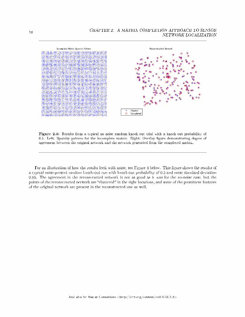
Figure 2.3: Results from a typical no-noise random knock-out trial with a knock-out probability of0.5. Left: Sparsity pattern for the incomplete matrix. Right: Overlay �gure demonstrating degree ofagreement between the original network and the network generated from the completed matrix.
For an illustration of how the results look with noise, see Figure 4 below. This �gure shows the results ofa typical noise-present random knock-out run with knock-out probability of 0.5 and noise standard deviation0.05. The agreement in the reconstructed network is not as good as it was for the no-noise case, but thepoints of the reconstructed network are �clustered" in the right locations, and some of the prominent featuresof the original network are present in the reconstructed one as well.
Available for free at Connexions <http://cnx.org/content/col11153/1.3>

19
Figure 2.4: Results from a typical noise-present random knock-out trial with a knock-out probabil-ity of 0.5 and a noise standard deviation of 0.05. Left: Sparsity pattern for the incomplete matrix.Right: Overlay �gure demonstrating degree of agreement between the original network and the networkgenerated from the completed matrix.
2.4.1.2 Realistic Knock-Out Trials
The �gures below, which show the results for the realistic knock-out trials, are similar to those above exceptthat they plot the average relative Frobenius-norm error over 25 trials versus maximum radius as opposedto fraction of unknown entries.
Available for free at Connexions <http://cnx.org/content/col11153/1.3>

20CHAPTER 2. A MATRIX COMPLETION APPROACH TO SENSOR
NETWORK LOCALIZATION
Figure 2.5: Simulation results for realistic knock-out trials without noise.
Available for free at Connexions <http://cnx.org/content/col11153/1.3>

21
Figure 2.6: Simulation results for realistic knock-out trials with noise present.
The most salient feature of these graphs is the odd �hump" that appears from radius values of about 0.5to 0.7, even in the no-noise case. Over this range, despite the fact that the radius is growing (meaning thatmore pairwise distances are known), the error in the completed matrix is actually becoming worse ratherthan better, which seems to contradict the excellent results discussed above for the random knock-out case.At the time of this writing, we are still unsure as to why this �hump" appears; however, we suspect that itmay have something to do with the OptSpace algorithm itself because when we run the same experimentusing the SVT algorithm of Candès, the hump does not appear, as the �gure below shows. (Note that,nevertheless, OptSpace tends to produce less error than SVT, even over the o�ending range of radii.)
Available for free at Connexions <http://cnx.org/content/col11153/1.3>

22CHAPTER 2. A MATRIX COMPLETION APPROACH TO SENSOR
NETWORK LOCALIZATION
Figure 2.7: OptSpace performance vs. SVT performance for realistic entry knock-out without noise.SVT does not display a �hump," but OptSpace generally returns better error values.
Perhaps more important than the �hump," however, is the fact that the scales on the axes of the abovegraphs alone are enough to demonstrate that the performance of the method in the realistic knock-out caseis decidedly worse than that for the random knock-out case. For example, consider the �gure below, whichshows the results of a typical no-noise, realistick knock-out trial with a maximum radius of 1. For thisparticular trial, over 97 percent of the pairs are known. The reconstructed network matches the originalquite well near the �center" of the network, but at the edges, the match becomes much worse. This behavioris not exhibited at all by random knock-out trials for comparable fractions of unknown entries, as the pictureat the bottom of the �gure illustrates, which was generated from a non-noise random knock-out trial inwhich 90 percent of the pairs were known.
Available for free at Connexions <http://cnx.org/content/col11153/1.3>

23
Figure 2.8: Results from a typical non-noise realistic knock-out trial with a maximum radius of 1. Top-Left: Sparsity pattern for the incomplete matrix. Top-Right: Overlay �gure demonstrating degree ofagreement between the original network and the network generated from the completed matrix. Bottom:Typical results from a non-noise random knock-out trial with knock out probability of 0.1 (90% of distancepairs are known).
Shrinking the radius only makes matters worse, as the next �gure illustrates. The maximum radius hereis√
2/2. Around 77 percent of the distance pairs are known, and yet the match is terrible.
Available for free at Connexions <http://cnx.org/content/col11153/1.3>

24CHAPTER 2. A MATRIX COMPLETION APPROACH TO SENSOR
NETWORK LOCALIZATION
Figure 2.9: Results from a typical non-noise realistic knock-out trial with a maximum radius of√
2/2.Left: Sparsity pattern for the incomplete matrix. Right: Overlay �gure demonstrating degree of agree-ment between the original network and the network generated from the completed matrix.
Adding noise only makes the results even worse. At �rst glance, this behavior appears to be inexplicable;however examining the sparsity patterns of the incomplete matrices reveals an interesting fact: the entryknock-out in the realistic case is far from being �random!" The sparsity patterns for the realistic knock-outmatrices reveal clear patterns of lines in their knocked-out entries that are not present in those for randomknock-out cases. This unintended regularity of entry selection violates the assumption made in all of thematrix completion literature that the known entries are taken from a uniform sampling of the matrix, so itwould seem that none of the theoretical results that have been derived apply in this case.
2.4.1.3 Conclusions
Our results show that matrix completion presents a viable means of approaching the sensor network local-ization problem under the assumption that the known pairs of distances come from a uniform sampling ofthe distance matrix. Under these conditions, matrix completion provides excellent network reconstructionand is fairly robust to noise. Unfortunately, its performance in the more realistic case in which distanceinformation will be excluded or included based on a maximum possible distance over which two sensors cancommunicate leaves much to be desired.
2.4.1.4 Future Work
With more time on this project, we would like to have explored the following questions further:
• What is the true origin of the mysterious �hump?" If it really is due to OptSpace as the above seemsto suggest, is there a way to modify the OptSpace algorithm to get it to go away?
• What is the fundamental reason that the realistic knock-out trials did not work? Is there a way to getthem to work better? (Perhaps something like permuting the distance entries in the matrix aroundto make the sampling pattern apparently more random would do the trick. If the permutations arestored somewhere, they can be undone after the matrix is completed if necessary.)
Available for free at Connexions <http://cnx.org/content/col11153/1.3>

25
• The experiment worked pretty well in two dimensions, at least for the random knock-out case. Willthree dimensions show results that are any di�erent?
2.5 Acknowledgments6
2.5.1 Acknowledgments
We would like to thank Mr. Andrew Waters for the invaluable support and guidance he provided us whilewe were working on this project as well as Prof. Baraniuk for suggesting such a fascinting project to us inthe �rst place.
2.6 References7
2.6.1 References
In addition to the papers that are cited throughout the other modules in this collection, we made use of thefollowing other resources when carrying out this project:
The OptSpace code written by Keshavan, Montanari, and Oh that was used for running the simulationscarried out in this project was obtained from http://www.stanford.edu/∼raghuram/optspace/code.html8 .While the multidimensional scaling code used to generate the plots of the reconstructed networks was writtenentirely by us, we made use of the following book for information on how to go about writing it:
I. Borg and P. Groenen. Modern Multidimensional Scaling: Theory and Applications. New York:Springer, 1997. pg. 207-210, 261-267.
6This content is available online at <http://cnx.org/content/m33142/1.1/>.7This content is available online at <http://cnx.org/content/m33146/1.1/>.8http://www.stanford.edu/∼raghuram/optspace/code.html
Available for free at Connexions <http://cnx.org/content/col11153/1.3>

26CHAPTER 2. A MATRIX COMPLETION APPROACH TO SENSOR
NETWORK LOCALIZATION
Available for free at Connexions <http://cnx.org/content/col11153/1.3>

Chapter 3
Discrete Multi-Tone Communication
Over Acoustic Channel
3.1 Introduction1
3.1.1 What is DMT and where is it used?
DMT is a form of Orthogonal Frequency Division Multiplexing. E�ectively, information is coded and mod-ulated by several di�erent sub carriers. This is the same modulation scheme used in common DSL channels.Speci�cally, at frequencies above those reserved for speech, there exist several hundred channels of the equalbandwidth used to transmit data to and from the internet. This is very convenient for phone users, as theseDMT channels can be easily �ltered out using a simple low-pass �lter, preventing any possible interferencefrom connecting to the internet while talking on the phone.
3.1.2 Why transmit over an acoustic channel?
The acoustic channel, and the audible frequencies contained therein, was chosen as a test area for our DMTproject simply because of its accessibility. No complex or expensive hardware is necessary to transmit overit, just a standard computer speaker and microphone setup.
3.1.3 What can DMT do for us?
As will be revealed in later modules, DMT modulation o�ers many features that protect our signal's in-formation from being distorted by the channel. Speci�cally, by transmitting our information over severalsubcarriers at the same time instead of just one carrier, we can use the frequency response of the system tosee which carriers are being attenuated and likewise increase the gain on those channels or get rid of themaltogether. You will discover, as we did, how di�cult that process turned out to be.
3.2 The Problem2
3.2.1 Creating a DSL Modem
Our goal is to use Discrete Multi-Tone modulation to transmit a text message over the audible range offrequencies in an acoustic channel. We are creating a DSL modem that transmits through the air.
1This content is available online at <http://cnx.org/content/m33147/1.1/>.2This content is available online at <http://cnx.org/content/m33155/1.1/>.
Available for free at Connexions <http://cnx.org/content/col11153/1.3>
27

28CHAPTER 3. DISCRETE MULTI-TONE COMMUNICATION OVER
ACOUSTIC CHANNEL
To do this, we will observe the frequency characteristics of the channel, and use that information toequalize our received transmission in hope to preserve the maximum amount of content from the signal. Asin any engineering problem, we are constantly striving to push the data-rate of our system, while minimizingthe occurrence of errors. Here we go!
The Transmitter (Section 3.3)The Channel (Section 3.4)Receiver (Section 3.5)Results and Conclusions (Section 3.6)
3.3 Transmitter3
3.3.1 Text to Binary Conversion
The �rst step is to convert our information into binary. We used the sentence �hello, this is our test message,�repeated four times, as our text message. To get it into binary, we used standard ASCII text mapping.
hello = 01101000 01100101 01101100 01101100 01101111
3.3.2 Series to Parallel
The next step is converting this vector of zeros and ones into a matrix. The vector is simply broken up intoblocks of length L, and each block is used to form column of the matrix.
3.3.3 Constellation Mapping
Now the fun begins. The primary method of modulation in DMT is by inverse Fourier Transform. Althoughit may seem counterintuitive to do so, by taking the inverse Fourier Transform of a vector or a matrix ofvectors, it e�ectively treats each value as the Fourier coe�cient of a sinusoid. Then, one could transmit thissum of sinusoids to a receiver that would in turn take the Fourier Transform (the inverse transform of theinverse transform, of course) and retrieve the original vectors.
But instead of taking the transform of our vectors of zeros and ones, we �rst convert bit streams of lengthB to speci�c complex numbers. We draw these complex numbers from a constellation map (a table of valuesspread out along the complex plane). See the �gure below for an example of a 4 bit mapping.
3This content is available online at <http://cnx.org/content/m33148/1.1/>.
Available for free at Connexions <http://cnx.org/content/col11153/1.3>

29
Constellation Mapping Table
Figure 3.1: This table shows which bit stream is mapped to which complex value.
3.3.4 Signal Mirroring and Inverse Fourier Transform
Why would we do that, you might ask. Doesn't converting binary numbers to complex ones just make thingsmore complicated? Well, DMT utilizes the inverse Fourier Transform in order to attain its modulation. Sotaking the IFFT of a vector of complex numbers will result in a sum of sinusoids, which are great signals tobe sending over any channel (they are the eigenfunctions of linear, time-invariant systems).
But before taking the inverse transform, the vectors/columns of the matrix must be mirrored and complexconjugated. The Inverse Fourier Transform of a conjugate symmetric signal results in a real signal. Andsince we can only transmit real signals in the real world, this is what we want.
3.3.5 Cyclic Pre�x
If we were transmitting over an ideal wire system, we would be done at this point. We could simply send itover the line and start demodulating. But with most channels, especially our acoustic one, this is not the case.The channel's impulse response has non-zero duration, and will therefore cause inter-symbol interference inour output.
Intersymbol interference occurs during the convolution of the input and impulse response. Since theimpulse response has more than a single value length, it will thus cause one block's information to bleed intothe next one.
Available for free at Connexions <http://cnx.org/content/col11153/1.3>

30CHAPTER 3. DISCRETE MULTI-TONE COMMUNICATION OVER
ACOUSTIC CHANNEL
To prevent this, we added what is called a cyclic pre�x to each block. As long as the length of the cyclicpre�x is at least as long as the impulse response, it should prevent ISI. However, it has a secondary e�ect aswell. We created the pre�x by adding the last N values of each block (where N is the length of the response)to the beginning, preserving the order. Doing this e�ectively converts the linear convolution of the impulseresponse with the block sequence to circular convolution with each block separately, since there will now bethe �wrap-around� e�ect. This will be handy later when we start characterizing the channel, since circularconvolution in time is equivalent to multiplication of DFT's in frequency.
00010110011010001 => 01000100010110011010001The �rst six bits in the second bit stream, 010001, is the cylcic pre�x. Note that although these values
are binary, they could essentially range from -1 to 1 since they sample the sinusoid sum that was formedafter inverse Fourier Transforming.
Please see the block diagram below. It summarizes the entire transmission process covered above.
Transmission Block Diagram
Figure 3.2: This diagram shows the all of the components and �ow of our transmission system.
Available for free at Connexions <http://cnx.org/content/col11153/1.3>

31
3.4 The Channel4
3.4.1 The Channel
To characterize the channel, we input an impulse by recording the tapping of the mic with our �ngers. Wethen played that sound through the speaker and recorded the response with the mic. The signal is below,along with its spectrum.
Impulse Response of the Channel and its Spectrum
Figure 3.3: These graphs characterize the channel that we are transmitting through
We did this in preparation for the receiving end of the system to divide the received signal's FFT by theimpulse response's FFT.
Below are plots of our transmitted and received signals, along with their spectrums. You will notice agreat similarity between the signals in time, however a distinct di�erence in frequency. Unfortunately, thisloss in frequency will translate to a loss of information.
4This content is available online at <http://cnx.org/content/m33144/1.1/>.
Available for free at Connexions <http://cnx.org/content/col11153/1.3>

32CHAPTER 3. DISCRETE MULTI-TONE COMMUNICATION OVER
ACOUSTIC CHANNEL
Transmitted and Received Signals in the time domain
Figure 3.4: These are the signals in time that we transmitted (green) and that we received (red). Asyou can see they look very similar, and take it from us, they also sound similar.
Transmitted and Received Signal Spectrums
Figure 3.5: The green spectrum is of the signal we transmitted, and the red is the spectrum of thesignal we received. We see a much bigger visual di�erence than we did in the time domain.
Above are plots for our transmitted and received signals. Here we used a block length of half the durationof the signal and sent it through the air at 44.1 kHz.
Available for free at Connexions <http://cnx.org/content/col11153/1.3>

33
3.5 Receiver5
3.5.1 Decoding the Transmission
Since the receiver has full knowledge of all the steps taken to transmit, the reception process is the exactinverse of transmission. The only di�erence is the addition of the channel equalization described in theprevious part. To get back the information we originally sent, we simply:
• Take the FFT of the reception and divide it by the FFT of the impulse response. Then iFFT it back.• Remove the cyclic pre�x• Take the Fourier Transform• Demirror the vector• Approximate each received value to nearest point in constellation and map them back to the original
bit sequences. See �gure below for example in 4 bit approximation.• Convert the binary series back to ascii letter equivalents.
Approximation of Constellation Map
Figure 3.6: The map on the left was approximated to the one on the right with a 2.15% percent error.
Please see the block diagram below. It summarizes the reception process.
5This content is available online at <http://cnx.org/content/m33151/1.1/>.
Available for free at Connexions <http://cnx.org/content/col11153/1.3>

34CHAPTER 3. DISCRETE MULTI-TONE COMMUNICATION OVER
ACOUSTIC CHANNEL
Receive Block Diagram
Figure 3.7: This diagram shows the all of the components and �ow of our receiver system.
3.6 Results and Conclusions6
ResultsUnfortunately, our microphone-speaker system was not successful in transmitting a text message. The
measured transfer function seemed reasonable since it modeled a low-pass �lter. But it was ine�ective inequalizing our received signal. This is most likely because the channel added far too much noise, in additionto attenuating many of the frequencies beyond recovery.
Since we were unable to acquire the desired results on bit-rate maximization and error minimization inthe acoustic channel, we created an arti�cial channel, using our observed frequency response plus Gaussiannoise. Modeling this channel in Matlab produced notable results. See the �gures below.
6This content is available online at <http://cnx.org/content/m33152/1.1/>.
Available for free at Connexions <http://cnx.org/content/col11153/1.3>

35
Bit-rate vs Block Length (2 and 4 bit)
Figure 3.8: This graph illustrates the fact that data rate increases as we increase block length. It alsoshows that a 4-bit scheme has twice the data rate of a 2-bit scheme, as one would expect.
Available for free at Connexions <http://cnx.org/content/col11153/1.3>

36CHAPTER 3. DISCRETE MULTI-TONE COMMUNICATION OVER
ACOUSTIC CHANNEL
Percent Error vs Block Length (2 and 4 bit)
Figure 3.9: This graph illustrates the fact that as block length increases so will the amount of errors.Also we see that the 4-bit scheme has a much greater amount of errors than the 2-bit.
These �gures indicate that both bit-rate and error-rate go up as block length increases. This makessense since increasing the block length increases the number of channels (Taking the iFFT of a longer signalproduces more unique sinusoids.). Squeezing more sinusoid carriers over the same bandlimited channel (0-22kHz) should result in more errors in demodulation, while transmitting more bits at the same time. It alsomakes sense that the 4 bit constellation mapping yielded higher bit-rates and error percentages since eachsinusoid carries more information, yet can more easily be approximated to the wrong constellation point.
The next project dealing with Discrete Multi-Tone modulation in the acoustic channel should certainlyinvolve a more professional recording system.
Available for free at Connexions <http://cnx.org/content/col11153/1.3>

37
3.7 Our Gang7
3.7.1 Gang Members
Dangerous Brian Viel �Electrical and Computational EngineeringSoarin' Dylan Rumph � Electrical and Computational Engineering
3.8 Acknowledgements8
We would like to thank:Jason Laska � Our project advisor for giving us moral support and steering us in the right direction.Rich Baraniuk � Hell, he taught us all we know about DSP2003 DMT Group (Travis White, Eric Garza, Chris Sramek) � We used much of their original matlab
code as a start for our modulation.
7This content is available online at <http://cnx.org/content/m33153/1.1/>.8This content is available online at <http://cnx.org/content/m33140/1.1/>.
Available for free at Connexions <http://cnx.org/content/col11153/1.3>

38CHAPTER 3. DISCRETE MULTI-TONE COMMUNICATION OVER
ACOUSTIC CHANNEL
Available for free at Connexions <http://cnx.org/content/col11153/1.3>

Chapter 4
Language Recognition Using Vowel PMF
Analysis
4.1 Meet the Team1
4.1.1 Language Recognition Using Vowel PMF Analysis
4.1.1.1 Meet the 4 Guys
Haiying Lu (hl6@) � Chinese boi from Mississippi. Likes sweet tea, fried chicken, and believes in true love.Dream occupation: Save the world with a law degree and lots of love.
Wharton Wang(wkw1@) �Culturally confused. 6'1 height complete waste. Fashion guru. Dream occu-pation: First Asian American President or win an Oscar, Grammy, & Tony.
Jason Xu (jax1@) � Hair never grows longer than one inch. Desires life to be like a musical. Diva. Dreamoccupation: Be the next Yao Ming or open his own gym.
Qian Zhang (qz1@) � Enjoys good tv shows and will critique your dance move. Campus celebrity. Dreamoccupation: Runway model or Pokemon Master.
1This content is available online at <http://cnx.org/content/m33133/1.2/>.
Available for free at Connexions <http://cnx.org/content/col11153/1.3>
39

40 CHAPTER 4. LANGUAGE RECOGNITION USING VOWEL PMF ANALYSIS
Figure 4.1
From L-R: Haiying Lu,Wharton Wang, Jason Xu, Qian Zhang
4.2 Introduction and some Background Information2
4.2.1 Introduction: Language Recognition Using Vowel PMF Analysis
In recent years, voice and sound recognition technology has become increasingly prevalent in general society.Early applications focused on security and privacy measures were utilized by a small portion of the totalpopulation. However, today virtually every person who owns a computer has access to such technology.There are programs which transcribe speech into text, identify di�erent speakers, identify what song is beingplayed, and accept audio signals as valuable input in general.
Our goal is to add language recognition to the growing list. The inspiration is from the multi-languagebackground of all the group members and about 60% of the Rice students speak at least two languages�uently. Therefore, we think it will be interesting to develop a system which can �listen� to a speech sampleand recognize the language it is using.
2This content is available online at <http://cnx.org/content/m33121/1.2/>.
Available for free at Connexions <http://cnx.org/content/col11153/1.3>

41
4.2.2 Background: Formant Analysis of Vowel Sounds
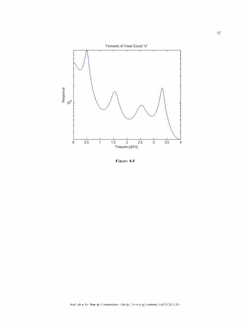
Formants are broad peak envelopes found in the spectrum of sound. Vowel sounds are pronounced with anopen vocal tract which creates a periodic resonance in air pressure. In contrast, consonant sounds require aclosure of the tract at some point during pronunciation, making them devoid of the same type of resonancefound in vowels. This results in easily identi�able di�erences between the two types of sounds in the frequencydomain�one of the most evident being the emergence of clear formants in vowels.
Each vowel sound generally has 3 or 4 formants located at speci�c frequency ranges corresponding tohow `open', `closed', `front', `back', or `round' the sound is. These characteristics depend on how the lips,tongue, and jaw are used in pronunciation. Although there are 3 or 4 total formants for most vowel sounds,the �rst two formants are usually all that is required to distinguish between them.
For our purposes of �nding PMFs of vowel sounds in di�erent languages, we are only looking at 5 mostbasic vowel sounds so it is usually su�cient to check up to the �rst two formants to decide the vowel sound.In addition to a vowel sound's natural frequency, the speaker's pitch will also vary the position of theformant. Therefore, we only used male speech samples consistently so that we have a relatively consistentvowel distribution for every sample.
4.3 Our System Setup3
4.3.1 Our System Setup
We plan to use the probability mass function (PMF) of 5 di�erent vowel sounds in 3 di�erent languages todetermine which language a speech sample is spoken in. However, before we can attempt to carry out thattask, we require a means of counting the number of occurrences of the 5 di�erent vowel sounds in any givenspeech sample to create the PMFs.
We chose English, Spanish and Japanese to analyze in this project. Spanish and Japanese both havesimple vowel sounds. For example, 90% of Japanese speaking consists of the 5 basic vowel sounds in ourdatabase. Spanish is similar and English is a little more complicated in pronunciation but we can still�nd an approximate distribution with our system and database. The choice of these languages has a goodrepresentation of western and eastern language and they are all widely used languages.
Two important databases are crucial in order for the system to perform at this point. One is the formant'sfrequency of the 5 most basic vowel sounds (a, i, u, e, o). The other database we want to have is the referencePMF of the 3 languages we are using. If we believe that there is a certain pattern in the PMF of the vowelsound distribution in these languages, then statistically, if we have a large enough sample, the PMF shouldrepresent the population parameters. In our case, we decided to use a long speech sample of each languageand use its vowel sound PMF as the reference data, which will be used later in the system to match smallerrandom speech samples.
3This content is available online at <http://cnx.org/content/m33115/1.1/>.
Available for free at Connexions <http://cnx.org/content/col11153/1.3>

42 CHAPTER 4. LANGUAGE RECOGNITION USING VOWEL PMF ANALYSIS
Figure 4.2
Figure 4.3
Available for free at Connexions <http://cnx.org/content/col11153/1.3>

43
4.4 Behind the Scene: From Formants to PMFs4
4.4.1 Identifying Vowel Sounds in a Speech Sample
We exploit each vowel sound's unique formant distribution to identify every occurrence of certain vowelsounds in a sample of speech. This was done by:
Inputting a speech sample � Since human speech typically maxes out at frequencies of 4 kHz, wechose to sample at 8000 Hz. This enabled us to compile our PMF data much more quickly than if we hadsampled at a higher standard of 44.1 kHz.
Windowing � A Hamming window is utilized to break our sample into separate chunks to be analyzedone at a time for the presence/absence of a vowel sound. Since the Hamming window slowly tapers towardszero at the edges, the spectrum will appear much smoother and less `jagged' than it would have had we useda rectangular window.
Figure 4.4
4.4.2 Frequency domain analysis of formants:
The code works as following:Locate the peaks, decide the formant according to the frequencies of 3 or more consecutive high magni-
tude, set �ags for the 5 vowel sound, go through the database to match, decide the vowel or consonant.Look at each window and determine whether or not there is a vowel there; a string of a certain vowel
sound (2 or more) will be treated as a `vowel', otherwise �not a vowel�. Then the system gives the output asa string of the �ve vowels: a, e, i, o, u and �C� if there is a consonant detected in between.
The plots below are generated by the code when we were building the formants data base using vowelsound samples.
4This content is available online at <http://cnx.org/content/m33134/1.3/>.
Available for free at Connexions <http://cnx.org/content/col11153/1.3>

44 CHAPTER 4. LANGUAGE RECOGNITION USING VOWEL PMF ANALYSIS
Figure 4.5
Available for free at Connexions <http://cnx.org/content/col11153/1.3>

45
Figure 4.6
Available for free at Connexions <http://cnx.org/content/col11153/1.3>

46 CHAPTER 4. LANGUAGE RECOGNITION USING VOWEL PMF ANALYSIS
Figure 4.7
Available for free at Connexions <http://cnx.org/content/col11153/1.3>
47
Figure 4.8
Available for free at Connexions <http://cnx.org/content/col11153/1.3>

48 CHAPTER 4. LANGUAGE RECOGNITION USING VOWEL PMF ANALYSIS
Figure 4.9
4.4.3 Creating Language PMFs
In order to create probability mass functions for the distribution of our 5 vowel sounds in di�erent languages,we �rst gathered several speech samples of di�erent languages. Since our code operates on .wav �les sampledat 8000 kHz, we re-sampled all of our speech samples to meet these speci�cations. Using our code, weidenti�ed how often the 5 sounds occurred in all of the samples of one language, and then created a probabilitymass distribution function based o� of that information.
function answer = langdetect(x)
%Transform the character string from formants.m to recognizable numerical
%values
x = double(x);
%Initiate count vector
count = zeros(5,1);
%Count the number of occurences for each vowel
for i=1:length(x)
if x(i) == 97
count(1) = count(1) + 1;
elseif x(i) == 101
count(2) = count(2) + 1;
elseif x(i) == 105
count(3) = count(3) + 1;
elseif x(i) == 111
count(4) = count(4) + 1;
Available for free at Connexions <http://cnx.org/content/col11153/1.3>

49
elseif x(i) == 117
count(5) = count(5) + 1;
else
continue;
end
end
%Normalize
count = count/(sum(count));
%PMF Bank
JAP = [0.25 0.35 0.12 0.23 0.05];
SPA = [0.06 0.45 0.19 0.2 0.1];
ENG = [0.15 0.35 0.05 0.4 0.05];
%Finding the difference between the sample and the reference
japdiff = abs(count'-JAP);
spadiff = abs(count'-SPA);
engdiff = abs(count'-ENG);
%Put the sum of the differences into a vector
diff = [sum(japdiff), sum(spadiff), sum(engdiff)];
%Find the index and magnitude of the minimum difference
[Y,I] = min(diff);
%Check and output which language has the lowest absolute difference
if I == 1
answer = 'Japanese';
elseif I == 2
answer = 'Spanish';
else
answer = 'English';
end
4.5 Results5
4.5.1 Detection
For each language, we prepared �ve samples for detection. In essence, our code compares the pmfs of thesample with the reference pmfs in our database. The most straightforward method is to subtract the samplePMF vector from the 3 reference PMF vectors in the database and look at the sum of the di�erence from 5vowels. The one with the smallest total error will be the output decision of the language.
Reference PMFs
a E i o u
JAP 0.25 0.35 0.12 0.23 0.05
SPANISH 0.06 0.45 0.19 0.2 0.1
ENGLISH 0.15 0.35 0.5 0.4 0.5
Table 4.1: Reference pmfs compiled from sixty minute samples for each language
5This content is available online at <http://cnx.org/content/m33113/1.2/>.
Available for free at Connexions <http://cnx.org/content/col11153/1.3>

50 CHAPTER 4. LANGUAGE RECOGNITION USING VOWEL PMF ANALYSIS
4.5.2 Results
Japanese
a e i o u
0.1866 0.4249 0.1593 0.2018 0.0273
0.2592 0.3723 0.1105 0.2020 0.0559
0.2606 0.3092 0.1238 0.2427 0.0635
0.2412 0.3496 0.1344 0.2092 0.0656
0.0816 0.3754 0.0727 0.3071 0.1632
Table 4.2: Pmfs generated from �ve �ve-minute Japanese samples
Spanish
a e i o u
0.1008 0.4258 0.2145 0.1398 0.1192
0.0396 0.4578 0.1887 0.2559 0.0580
0.0506 0.454 0.1902 0.1979 0.1074
0.0682 0.4763 0.1630 0.2187 0.0738
0.0608 0.4053 0.2055 0.1929 0.1355
Table 4.3: Pmfs generated from �ve �ve-minute Spanish samples
English
a e i o U
0.1580 0.3553 0.0769 0.3764 0.0335
0.1830 0.2468 0.1450 0.3021 0.1231
0.1798 0.4568 0.1023 0.2029 0.0582
0.1013 0.5023 0.0803 0.2587 0.0287
0.1670 0.3897 0.0598 0.3667 0.0168
Table 4.4: Pmfs generated from �ve �ve-minute English samples
Detection Results
Sample1 Sample2 Sample3 Sample4 Sample5
Japanese Japanese Japanese Japanese Japanese English
Spanish Spanish Spanish Spanish Spanish Spanish
English English Japanese Japanese Spanish English
Table 4.5: Detection results of the �ve samples of each language
Available for free at Connexions <http://cnx.org/content/col11153/1.3>
51
4.6 Conclusions6
4.6.1 Conclusions
After generating the PMFs from samples of each language, we notice that, for Japanese, the probability ofthe �u� sound is comparatively smaller than the other vowel sounds. This supports the fact that �u� soundis actually quite uncommon in the Japanese language. In addition, from our generated pmfs, it appearsthat detection for Japanese is fairly consistent, with only one sample missed. For Spanish, each of the �vesamples was detected correctly. However, for English, only two of the �ve samples were detected correctly.This result may suggest that English has greater variability in its vowel sounds than Spanish and Japanese.Therefore, �ve-minute samples are not enough for proper detection.
We conclude that our approach is inadequate for proper language detection. First, the PMFs of vowelsounds for di�erent languages do not vary as much as we initially thought. Therefore, languages of similarorigins (e.g. romantic languages) are di�cult to di�erentiate apart. Second, our approach is extremelysample-size dependent, because it relies on the sample PMF to converge to the reference PMF. By the law oflarge numbers, our approach would only work with large sample sizes. In addition, there is no guarantee thatour reference PMF is the expected PMF of the language. We compiled our reference PMF from sixty totalminutes of samples, but the actual expected PMF may require much larger samples. Third, our method isquite tedious. Our samples require signi�cant signal processing before it can be used in our system, includingdown-sampling, ampli�cation, and noise removal. Also, each person speaks at di�erent formant frequencies.Therefore, the vowel sound recognition system needs to be synced to each speaker. In conclusion, ourlanguage detection system is functional but severely limited.
4.6.2 Improvements
There's always room for improvement! As mentioned, a larger sample size would greatly improve theaccuracy of our system. In addition, since what separate languages are not their vowels but consonants,I believe a consonant sound recognition system in complement with our vowel sound recognition systemwould drastically improve the applicability of our system. Finally, the detection process, especially thepreparation of the speech samples, can be automated to lessen hardship on the tester.
4.6.3 Acknowledgements
We would like to extend our thanks to Professor Richard Baraniuk, Matthew Moravec, Daniel Williamson,and our mentor Stephen Schnelle.
6This content is available online at <http://cnx.org/content/m33127/1.3/>.
Available for free at Connexions <http://cnx.org/content/col11153/1.3>

52 CHAPTER 4. LANGUAGE RECOGNITION USING VOWEL PMF ANALYSIS
Available for free at Connexions <http://cnx.org/content/col11153/1.3>

Chapter 5
A Flag Semaphore Computer Vision
System
5.1 A Flag Semaphore Computer Vision System: Introduction1
5.1.1 A Flag Semaphore Recognition System
We seek to implement a computer vision system for classifying and interpreting �ag semaphore systems,as recorded by something as simple and commonplace as a webcam. The classi�cation is implemented ina MATLAB script that, taking an input video �le in wmv format, produces a string of the message insemaphore in the video. This can optionally produce a marked-up video, showing the semaphores as theyare recognized, overlaid with the video. Note that this can process video �les faster than they can be played,and could be implemented in realtime with parallel capture methods.
We also seek to implement a related Internet Engineering Task Force protocol documented in RFC 4824.This documents transmitting IP datagrams over a link layer implemented in �ag semaphore. We seek tobridge this link layer and a more standard Ethernet connection.
5.1.1.1 A Maritime Signaling System
Flag semaphore is a perhaps-archaic system for transmitting signals through a line of sight connections withdi�erent positions of colored �ags. With one �ag in each arm, and eight possible positions for each �ag, thereare 28 possible static signals with distinct positions for each �ag, with an additional �attention� dynamicsignal, and space, denoted with both �ags down.
The traditional naval semaphore �ags, as used in the system we have implemented are square, are squareand are divided into two large red and yellow triangles across the diagonal. Because the �ags are not rigid,they deform, making traditional matched �ltering di�cult, but the colorful design of the �ags is helpful,because it allows us to use color tracking to determine the �ags' positons.
1This content is available online at <http://cnx.org/content/m33092/1.2/>.
Available for free at Connexions <http://cnx.org/content/col11153/1.3>
53

54 CHAPTER 5. A FLAG SEMAPHORE COMPUTER VISION SYSTEM
Figure 5.1: A diagram of signal "J" (courtesy of Wikipedia). This symbol is always used to begintransmission.
5.2 A Flag Semaphore Computer Vision System: Program Flow2
5.2.1 Program Computational Flow
This section describes the processes that the �ag semaphore computer vision system we implemented un-dergoes in order to process input signals an produce output, separating the description into sections aboutthe input, classi�cation, and ouput. Refer to the �ow chart in Figure 5.2 for an illustration and concisedescription.
Figure 5.2: This �ow chart illustrates the processes involved in the �ag semaphore computer visionsystem from input signal to various outputs.
2This content is available online at <http://cnx.org/content/m33095/1.2/>.
Available for free at Connexions <http://cnx.org/content/col11153/1.3>

55
5.2.2 Input
The �ag semaphore computer vision and interpretation system we developed takes a prerecorded video �leas input to a MATLAB function. The video signal should be produced with two semaphore signaling �agsof the red and yellow triangle type. For best performance, the signaler should be near the center of thevideo frame images and as close to the camera as possible while ensureing that the vertical and horizontalsignaling range �ts within the images. The signaler may either signal facing the camera or signal facing awayfrom the camera, and the proper adjustment will automatically be made by the program. Also, The upwarddirection of the camera must correspond to the upward direction of the signaler.
All signals should be formed through rapid motion to the desired �ag positions. A signal is only guaran-teed to register if it is held in place for at least the speci�ed hold time (which defaults to 1 second). However,the framerate of the video �le and the rate at which a person can signal limit the signaling rates compati-ble with this program to reasonable values. Increasing the hold time increases the accuracy of the output.Repeated characters should be formed by signaling a space between them. Please note that the "chip-chop"attention signal is not supported at this time. (It is an error in the RFC 4824 protocol.) Every signal mustbegin with the alphabetic character (J) on the �rst frame, which is used to determine the direction thesignaler is facing and the pixel position of the signaler. This �rst character will not be displayed.
The video �le itself should be in a wmv format, although other �le types compatible with mmread mayalso function correctly. The �le should be placed in the same directory as this �le (FlagSemaphore.m) andthe �le name should be passed to the function in a string as the �rst arguement.
The second arguement, which is optional, supplies the desired time, in seconds, for which a signal mustbe held in order to be guarenteed to register. Increasing this parameter decreases the likelihood that aslow transition between two signals will be incorrectly registered as a signal, but decreases the best possiblesignaling rate. Thus, signal transitions should be fast and abrupt for this reason. The default hold time isone second.
5.2.3 Classi�cation
The �ag semaphore computer vision and interpretation system we developed, after extracting half of thehold time blocks of input video data as RGB matrices, classi�es the signal as a �ag semaphore symbol andthen produces several forms of output. Because of the objects of interest in the image are two bright redand yellow �ags, the classi�cation problem suggests color tracking as a promising approach.
Hence, our classi�er begins by performing color matching with the RGB matrix data of each frame in thehalf of the hold time interval in order to �nd the red regions and yellow regions in the image. Color matchingis a somewhat di�cult problem since the RGB regions corresponding to a given color are, in general, notconvex and di�cult to describe algorithmically. However, our rudimentary color matching algorithm wasalways su�cient to highlight the �ag regions.
Because there are multiple �ags in the image and there could be similarly colored objects nearby, we usea 2D matched �lter with a small square box as the �ltering signal implemented in the frequency domainfor speed in order to discriminate between objects of the same color. A simple peak �nding algorithm then�nds the pixel locations of the red objects and the pixel locations of the red objects. Since our �ags arered and yellow, we search for red objects near yellow objects and identify those as �ags, with special casehandling so that the cases in which less than two red objects or less than two yellow objects are found maystill be correctly identi�ed using saved data from the previous �ag locations. This produces results that arehighly resistant to noise contamination unless the noisy objects are colored with large patches of both redand yellow.
Each of the �ag positions are then placed in one of eight angular regions about an estimate of the centerof the signaler corresponding to the eight �ag positions used to form �ag semaphore signals. If the �agsremain in the same angular region for the vast majority of the frames considered, the �ags are not in motionand a symbol is registered according to which angular regions contain the �ags. Otherwise, the �ags aretaken to be in transition. Thereafter, the output symbol is interpreted in the context of the sequence ofprevious symbols to produce a character or to toggle between letters and numbers.
Available for free at Connexions <http://cnx.org/content/col11153/1.3>

56 CHAPTER 5. A FLAG SEMAPHORE COMPUTER VISION SYSTEM
5.2.4 Output
Several other inputs can optionally be supplied to specify other options. The print �ag is the secondargument and determines whether the interpreted message will be displayed on the MATLAB prompt. Thethird argument is the play �ag which speci�es whether the video will be played in a MATLAB �gure window.The fourth argument is the transceiver �ag which determines whether the program will attempt to send andreceive TCP/IP packets (currently ignored). The �nal two arguments determine whether an output video�le will be produced and specify the name of the output �le. For information on how to form packets ofTCP/IP data, refer to the RFC 4824 documentation3 .
For example, the following would store a the message interpreted from the video �le example1.wmv intothe string message1 without printing to the MATLAB prompt, playing the video �le, attempting to transmitand recieve packets, or writing an output video �le.
message1=FlagSemaphore('example1.wmv');
This, on the other hand, would store a the message interpreted from the video �le example2.wmv intothe string message2 while printing to the MATLAB prompt but not playing the video �le, attempting totransmit and recieve packets, or writing an output video �le.
message2=FlagSemaphore('example2.wmv',1,1,0,0,0,'');
This, example would store a the message interpreted from the video �le example3.wmv into the stringmessage3 while playing the video �le but not printing to the MATLAB prompt, attempting to transmit andrecieve packets, or writing an output video �le.
message3=FlagSemaphore('example3.wmv',1,0,1,0,0,'');
This, example would store a the message interpreted from the video �le example4.wmv into the stringmessage4 while attempting to transmit and recieve packets but not playing the video �le, printing to theMATLAB prompt, or writing an output video �le. Note that this option is not yet implemented and will beignored.
message4=FlagSemaphore('example4.wmv',1,0,0,1,0,'');
This, example would store a the message interpreted from the video �le example5.wmv into the stringmessage5 while writing an output video �le but not playing the video �le, printing to the MATLAB prompt,or attempting to transmit and receive packets.
message5=FlagSemaphore('example5.wmv',1,0,0,0,1,'exampleoutput5.wmv');
Some example �ag semaphore signal input video �les and output video �les can be found in the demon-strations section. Links to the full source code can be found in the additional resources section.
5.3 A Flag Semaphore Computer Vision System: ProgramAssessment4
5.3.1 Program Approach Advantages
The approach taken to the implementation of our �ag semaphore computer vision classi�cation and inter-pretation system described in the program �ow module provides several important bene�ts.
Due to the use of the Fast Fourier Transform to implement the matched �lter in the frequency domain,the program runs su�ciently fast that it could be used for real time video processing with the aid ofadditional parallel video capture software, such as that which can be found in the MATLAB Data Acquisition
3http://tools.ietf.org/html/rfc48244This content is available online at <http://cnx.org/content/m33098/1.2/>.
Available for free at Connexions <http://cnx.org/content/col11153/1.3>

57
Toolbox. When additional speed is desired, we note that the program remains highly accurate, even with adownsampling factor of three in both spacial dimensions.
Furthermore, the program demonstrates robustness when presented data contaminated with noise in theform of extraneous red or yellow objects as a result of the use of both the red and yellow region data whenattempting to identify the �ags. Detailed special case handling prevents video frames in which one or morecomplete color region of a �ag is occluded from ruining the color tracking.
Although it is di�cult to get a good estimate of the accuracy of the classi�er, limited testing, whichcan be seen on the demonstrations page, suggests that the results are quite accurate. Additionally, theprogram provides for variable accuracy by increasing or decreasing the signal hold time parameter Thisboosts accuracy by reducing the likelihood that a transition between symbols will be classi�ed as a symbolbut decreases the maximum possible signaling rate due to increased required pause time at each symbol.Hence this option represents a tradeo�, the optimal value of which will be di�erent for di�erent signalers.
5.3.2 Program Approach Disadvantages
Although su�ciently e�ective for the test videos, the color matching and peak detection algorithms used arenot perfect. A full treatment of color matching would be somewhat di�cult as RGB regions correspondingto a given color are, in general, not convex and thus di�cult to describe. The solutions used are ad hocsolutions that we developed for the problems of color matching and peak detection, so there likely existsuperior algorithms to perform those tasks.
Also, the program models the signaler arms as rotating about a single point, but there is width betweenhuman shoulders. While this problem was e�ectively overcome with empirical adjustment of the size of theangular regions by observation of signaler habits, it remains a weakness of the model.
Occasionally incorrect signaling due to signaler error makes it di�cult to get a good estimate of theaccuracy of the classi�er, but the program works well for some hold time for every test signal video recorded.
5.4 A Flag Semaphore Computer Vision System: Demonstration5
5.4.1 Example Video Input and Output
In the testing of the recognition system, several basic signals were recorded. These tested things like rec-ognizing the position of the sender from the �rst semaphore "J". This is essential to properly recognize alleight positions of the �ags, each of which occurs in our test signals. We also test the letters to numbers statetransition.
Example 5.1
Example Input Video: ELEC 301
This media object is a Flash object. Please view or download it at<http://www.youtube.com/v/uU3_7cNT_7U&hl=en_US&fs=1&>
Figure 5.3: A sample signal that spells out the course number ELEC 301, which includes both lettersand numbers.
5This content is available online at <http://cnx.org/content/m33100/1.2/>.
Available for free at Connexions <http://cnx.org/content/col11153/1.3>

58 CHAPTER 5. A FLAG SEMAPHORE COMPUTER VISION SYSTEM
Example Output Video: ELEC 301
This media object is a Flash object. Please view or download it at<http://www.youtube.com/v/5EeiXKrKwC8&hl=en_US&fs=1&>
Figure 5.4: The output of the the �lter for the signal "ELEC 301 " above. Notice the blank outputfor the control codes for letters (the �rst) and numbers. This �le is output directly from the MATLABcode.
Example 5.2
Example Input Video: ABCDEFG
This media object is a Flash object. Please view or download it at<http://www.youtube.com/v/IbJ2fDOtUVs&hl=en_US&fs=1&>
Figure 5.5: A simple alphabetic test case of the �ag semaphore recognition system. Note some of thepatterns formed in the standard semaphore alphabet.
Example Output Video: ABCDEFG
This media object is a Flash object. Please view or download it at<http://www.youtube.com/v/EC-3Ql_983c&hl=en_US&fs=1&>
Figure 5.6: The output of the recognition system for the signal "ABCDEFG". Note that the systemcorrectly di�erentiates between the signals, even when little motion is involved.
Example 5.3
Example Input Video: WRC
This media object is a Flash object. Please view or download it at<http://www.youtube.com/v/KgqXqYYVEpI&hl=en_US&fs=1&>
Figure 5.7: A short test signal "WRC". This was our �rst test case, and performs well.
Available for free at Connexions <http://cnx.org/content/col11153/1.3>

59
Example Output Video: WRC
This media object is a Flash object. Please view or download it at<http://www.youtube.com/v/LB4jJqiV0-A&hl=en_US&fs=1&>
Figure 5.8: The system correctly handles this three-letter signal.
5.5 A Flag Semaphore Computer Vision System: TCP/IP6
5.5.1 A Link-Level Layer for IP Transmissions
The idea of using �ag semaphore to transmit Internet Protocol packets is suggested in RFC 4824[4]. Thispresents a link-layer protocol, suitable for encapsulating and transmitting IP packets, analogous to theEthernet protocol frequently used for wire transmissions between machines, described by RFC 894[5] andother Internet Engineering Task Force (ITEF) standards.
This protocol was presented as a Request For Comments on April �rst, 2007. To our knowledge, noworking implementation of this protocol has been implemented, although several errata in the originalpublication have been identi�ed. A similar protocol, RFC 1149, which transfers IP datagrams over aviancarriers, was successfully tested in 2001 by a Linux User Group in Bergen, Norway[8], more than ten yearsafter the original speci�cation was published.
Having implemented a �ag semaphore recognition system, it seems reasonable to attempt to use it toimplement the protocol described in RFC 4824. It even seems reasonable to attempt to write a IP-SFS toEthernet bridge, but technical limitations prevented the completion of the bridge functionality. A completereceiver and transmitter framework exists, although the handling of states is incomplete.
5.5.1.1 IP-SFS Channel Design in Summary
The suggested channel protocol uses 25 of the alphabetic symbols in the standard semaphore alphabet. The�rst 16 characters are reserved for data transmission, and the remaining 9 are used for channel control codes.
The interface is half-duplex, in that an interface may be either idle, transmitting, or receiving. The idlestate is characterized by occasional KAL keep-alive signals, and either interface can initiate a state changefrom idle to transmitting by sending a RTT signal.
5.5.1.2 Decoding IP-SFS Packets
In an incoming IP-SFS character stream, as with the one created by our MATLAB interface. We can usean internal state machine, which encodes frames as strings between FST and FEN signals, with charactersdeleted by the appropriate FUN or SUN undo signals. Note that this reception is received asynchronously, ina separate instance if IpSfssRx, so that decoding bottlenecks will not a�ect our semaphore receiver.
Once an entire packet is received, and control signals are stripped out, it is possible to condense oursemaphore sequence to a byte array, as each signal represents a 4-bit nibble. A small amount of bytemanipulation shifts each pair of semaphores into a single byte. Note that the number of semaphores receivedmust be even.
The �rst two and last two bytes of each IP-SFS frame are header and footer data � the header de�nesone of �ve possible encapsulated protocols with support for compressed or uncompressed IPv4 or IPv6, and
6This content is available online at <http://cnx.org/content/m33094/1.2/>.
Available for free at Connexions <http://cnx.org/content/col11153/1.3>

60 CHAPTER 5. A FLAG SEMAPHORE COMPUTER VISION SYSTEM
an optional cyclic redundancy check method � CRC CCITT 16, a standard polynomial redundancy checkthat is easy to implement. The last two bytes of the frame are the checksum of the frame so far.
The IpSfssFrame class can be constructed using a string � such a sequence of data semaphores. Thiswill throw an exception in case of error, or create an instance of the frame. Errors are thrown for formatviolations or CRC failures. The object allows us to return the encapsulated packet as a byte array.
5.5.1.3 Sending IP-SFS Packets
The system also supports the propagation of IP datagrams. An IpSfssFrame can also be instantiated witha raw IP packet with any of the standard options, including compression and verifying checksums.
An asynchronous transmitter, IpSfssTx, can be instantiated. Running this in a separate thread allowssemaphores to be queued, without the function blocking for completion. This is especially important becausethere is a (con�gurable) minimum display time for each signal. A Swing-based GUI can display these signalson the screen.
5.5.1.4 IP-SFS to Ethernet Bridge
The original goal was to produce an IP-SFS to Ethernet bridge, such that IP packets transmitted as thepayload of SFS frames could be placed onto the outgoing queue of a running machine with a networkconnection.
Such �raw sockets� does not natively exist on Windows, although the WinPcap project o�ers link-layeraccess. The link-layer access, however, requires proper Ethernet headers on outgoing packets, which couldlikely be fabricated with additional time spent on the project.
The Java libpcap interface also o�ers methods to dump incoming packets to a �le. This makes networksni�ng possible, but does not allow packets to be read in real time.
5.5.1.5 Future Expansion
Because of time and scope constraints, the IP-SFS to Ethernet bridge was not satisfactorily completed. Inthe future, expanding this to full functionality would be quite an interesting project.
It should also be noted that much of the IpSfssFrame functionality was written in haste, and while itwas tested on reasonable cases, more automated unit testing on this and other classes in the Java IP-SFSframework would be ideal.
The internal state of the transceiver is also partially incomplete. It does not respect the state (transmit-ting, receiving, idle), of the connection, nor does it acknowledge packet receptions with ACK signals (or NAKon errors), because the receiver and transmitter are not su�ciently connected.
5.6 A Flag Semaphore Computer Vision System: Future Work7
5.6.1 Real Time Video Processing
The �ag semaphore computer vision and interpretation program that our group has a reasonably fast runtimedue to the use of a matched �lter implemented in the frequency domain and the accuracy of the programunder spatial downsampling. In fact, the program runs in considerably less time than the duration ofinput video �le provided that the program is not also attempting to write an output video �le, clockingapproximately 15 seconds for an approximately 20 second video. Consequently, this video processing couldbe performed in real time with the aid of video capture software operating in parallel, such as is providedin the MATLAB Data Acquisition Toolbox. However, due to a lack of funds, this was not implemented andleft as a possible future addition that would require very little modi�cation to our existing code.
7This content is available online at <http://cnx.org/content/m33103/1.2/>.
Available for free at Connexions <http://cnx.org/content/col11153/1.3>

61
5.6.2 Identi�cation of all Symbols
While we could successfully identify all of the static symbols in the �ag semaphore symbol set, we left the�chip-chop� attention symbol unidenti�ed as it is not used under the RFC 4828 TCP/IP standard and itsexclusion greatly simpli�ed the code. However, any future modi�cations may wish to support its identi�cationfor completeness.
5.6.3 TCP/IP Transceiver Implementation
Because of time and scope constraints, the IP-SFS to Ethernet bridge was not satisfactorily completed. Inthe future, expanding this to full functionality would be quite an interesting project. It should also be notedthat much of the IpSfssFrame functionality was written in haste, and while it was tested on reasonablecases, more automated unit testing on this and other classes in the Java IP-SFS framework would be ideal.The internal state of the transceiver is also partially incomplete. It does not respect the state (transmitting,receiving, idle), of the connection, nor does it acknowledge packet receptions with ACK signals (or NAK onerrors), because the receiver and transmitter are not su�ciently connected.
5.6.4 Miscellaneous
Other possible future expansions and modi�cations of our program could include improvements in the colormatching and peak detection algorithms used to determine the positions of the �ags. Although the currentversions function correctly with a high degree of accuracy, they are ad hoc solutions that we developed tothe problems of color matching and peak detection, so there may exist superior algorithms to perform thosetasks. Further optimization of code for improved speed performance is desirable in order to perform both realtime processing and real time video output writing to make the program more useful even if it is impractical.
5.7 A Flag Semaphore Computer Vision System: Acknowledgements8
5.7.1 Acknowledgements
The authors would now like to acknowledge some of the other people who have contributed to the successof this project. First, we thank Chinmay Hegde and Dr. Rich Baraniuk for mentoring our project groupand instructing our ELEC 301 class, respectively. We also appreciate Dr. Alan Cox for providing us withinformation on the use of raw TCP sockets. Finally, we send our thanks to Micah Richert who published aprogram enabling our old version of MATLAB to read and write from wmv �les and to the jNetPcap andWinPcap developers for their e�orts.
5.8 A Flag Semaphore Computer Vision System: AdditionalResources9
5.8.1 Semaphore Related Resources
• A section10 of the 1913 Royal Navy Handbook of Signaling is available from the World War I DocumentArchive.11
• RFC 482412 documents sending IP datagrams over �ag semaphore.
8This content is available online at <http://cnx.org/content/m33106/1.2/>.9This content is available online at <http://cnx.org/content/m33107/1.2/>.
10http://www.gwpda.org/naval/s0900000.htm11http://gwpda.org/12http://tools.ietf.org/html/rfc4824
Available for free at Connexions <http://cnx.org/content/col11153/1.3>

62 CHAPTER 5. A FLAG SEMAPHORE COMPUTER VISION SYSTEM
5.8.2 Project Resources
• The SourceForge13 project page for our project is available: A Flag Semaphore Computer VisionSystem.14
• The videos15 for the project are available on YouTube.
5.9 A Flag Semaphore Computer Vision System: Conclusions16
5.9.1 Conclusions
Over the course of the past month, our project group successfully implemented a computer vision systemfor the interpretation of �ag semaphore signals. The approach taken has yielded accurate results that arerobust under noise contamination and can withstand substantial spacial downsampling. However, weaknessesin color matching and peak detection along with several missing desirable features leaves room for futureimprovement. Notably, the program would be capable of processing video input in real time with the aidof parallel video capture software with few additional changes to the code. Also, signi�cant progress towardfully implementing a TCP/IP packet transceiver using the RFC 4824 standard was made. Our limited testingresults suggest that the program yields results that are of reasonably high accuracy, with a tradeo� betweenaccuracy and signaling rate. Hence, we conclude with the primary demonstration of our projects success inthe output video below that signals the class name �ELEC 301�.
Example Output Video: ELEC 301
This media object is a Flash object. Please view or download it at<http://www.youtube.com/v/5EeiXKrKwC8&hl=en_US&fs=1&>
Figure 5.9: The output of the the �lter for the signal "ELEC 301 " above. Notice the blank outputfor the control codes for letters (the �rst) and numbers. This �le is output directly from the MATLABcode.
13http://sf.net14http://sourceforge.net/projects/�agsemaphore/15http://www.youtube.com/user/smkruzick16This content is available online at <http://cnx.org/content/m33109/1.2/>.
Available for free at Connexions <http://cnx.org/content/col11153/1.3>

Chapter 6
License Plate Extraction
6.1 Prelude1
6.1.1 Purpose
To develop an algorithm for extraction of license plate numbers from still photos of stationary cars.
6.1.2 Methods
We divided this project into two sections- Image Processing and Support Vector Machine (SVM) Training:
• We take picture of a still car (from either front or back), compress and crop out to speed up the process,localize the plate position and extract the letters into individual binary matrices.
• We take each of the matrix generated in the previous process and use the SVM algorithm to distinguishwhich letter exactly it is.
6.1.3 Applications
This algorithm can be integrated to the related vehicle identi�cation applications such as:
1. Parking lot registration2. Tra�c violation tracking3. Vehicle surveillance
6.2 Image Processing - License Plate Localization and LettersExtraction2
The general method we used for extracting the license plate letters out of a picture was:
1This content is available online at <http://cnx.org/content/m33154/1.2/>.2This content is available online at <http://cnx.org/content/m33156/1.2/>.
Available for free at Connexions <http://cnx.org/content/col11153/1.3>
63

64 CHAPTER 6. LICENSE PLATE EXTRACTION
Figure 6.1: Overall method for �nding license plate letters/numbers.
1. Compression and Cropping: decreases the size of the photo and and blacks out areas that de�nitelydo not contain license plate.
2. License Plate Localization: determines the location of the plate in the photo3. Letter Extraction: searches within the plate for the plate letters/numbers and copies them out of
the photo.
Following is an explanation of the individual sections. Included are also images showing the e�ects of eachsection on the following picture:
Figure 6.2: Original image.
6.2.1 Compression and Cropping
In order to decrease image processing time, we �rst compress all pictures to a standard size and black outall areas that are de�nitely not license plates. The size we chose was 640px by 480px, the smallest size atwhich we could still reasonably read the license plates.
Available for free at Connexions <http://cnx.org/content/col11153/1.3>

65
To determine which areas were de�nitely not license plates, we realized that the typical Texas platecontained red, blue, and white as major colors. Therefore, we focused on these two colors, making ourcropping algorithm:
1. Separate the JPEG picture into its three layers of red, green, and blue.2. Consider the area around a blue pixel, and black it out if the density of red is lower than a certain
threshold value.
Figure 6.3: Compressed and cropped image (Note the black areas around the right and bottom of thephoto).
6.2.2 License Plate Localization
Once we determined which areas possibly contained license plates, we looked in those areas for the platesthemselves. We determined that most plates contain dark letters on light backgrounds and so looked forareas of high contrast.
Our �nal algorithm looked as follows:
1. Turn the cropped photo into black-and-white for easier di�erentiation between dark and light spots.2. Filter the image to remove noise (single-pixel white spots).3. Locate the license plate position by scanning the photo vertically. We expect a row running through
the license plate row to have a maximum number of individual dark spots, or "clusters." Therefore, we�nd and store the two rows in the image with that contain the most clusters.
4. To �nd the horizontal position of the plate, scan the picture horizontally by moving a square windowfrom left to right and counting the number of clusters inside. The �nal position of the license plate issquare that contains the greatest number of clusters. If any two squares contain the same number ofclusters, the two are merged together.
Available for free at Connexions <http://cnx.org/content/col11153/1.3>

66 CHAPTER 6. LICENSE PLATE EXTRACTION
Figure 6.4: Close-up of the license plate as determined by the algorithm.
6.2.3 Letter Extraction
To �nd the letters on a license plate, we �rst determined some identifying characteristics:
1. Usually, and always on Texas plates, the letters of the plate are dark on a light background.2. The letters are uniform in height3. The letters all occur in approximately the same area.4. There are usually between 3 and 7 letters on a plate.
These characteristics give us the form for our letter extracting algorithm.
1. From the plate-locating algorithm, we have a small 200px by 200px image that contains the car's licenseplate.
2. We convert the image into grayscale for easier processing.3. We locate all the dark (low intensity) spots in the picture that are surrounded by light (high intensity)
spots. We determine the separation between these dark spots and give each individual spot a label.4. Compare the sizes of the spots and look for about six that have the same height. These six spots are
the letters on the plate.5. Save the pixels that make up the letters into their individual matrices.
We tried this algorithm and found that it worked for all images for which the plate-locating algorithmreturned an image containing the entire plate.
Available for free at Connexions <http://cnx.org/content/col11153/1.3>

67
Figure 6.5: Letters extracted from the photo.
6.3 SVM Train3
6.3.1 The Math and Algorithm
For digit recognition, we use Support Vector Machine (SVM) as a learning machine to perform multi-classclassi�cation.
The way SVM works is to map vectors into an N-dimensional space and use an (N-1)-dimensional hy-perplane as a decision plane to classify data. The task of SVM modeling is to �nd the optimal hyperplanethat separates di�erent class membership.
Example 6.1Let's take a look at a simple schematic example where every object either belongs to GREEN orRED.
Figure 6.6: Picture from: Chih-Chung Chang and Chih-Jen Lin, LIBSVM : a library for support vectormachines, 2001.
SVM �nds the line de�ning the boundary between the two types. Then, it can classify a newobject by looking at on which side of the line it falls.
However, it is unlikely that we can always have a linear dividing boundary. Rather than �ttingnonlinear curves to the data, we can map each object into a di�erent space via a kernel functionwhere a linear dividing hyperplane is feasible.
3This content is available online at <http://cnx.org/content/m33159/1.2/>.
Available for free at Connexions <http://cnx.org/content/col11153/1.3>

68 CHAPTER 6. LICENSE PLATE EXTRACTION
Figure 6.7: Hyperplane classifying the two cases (Picture from: Chih-Chung Chang and Chih-Jen Lin,LIBSVM : a library for support vector machines, 2001.)
The concept of the kernel mapping function is so powerful that SVM can perform separationwith very complex boundaries. The kernel function we use in this project is radial basis function(RBF).
6.3.1.1 SVM Working Principles
• Vectorize each instance into an array of features (attributes).• Model with training data to �nd optimal dividing hyperplane with maximal margin.• Use SVM to map all the objects into a di�erent space via a kernel function (see Figure 3 for examples).• Classify new object according to its position with respect to hyperplane.• Errors in training are allowed while the goal of training is to maximize the margin and minimize errors.
Namely, �nd the solution to optimization problem in Figure 4, where x is the attribute, y is the objectlabel, ξ is the error and φ is the mapping function.
Available for free at Connexions <http://cnx.org/content/col11153/1.3>
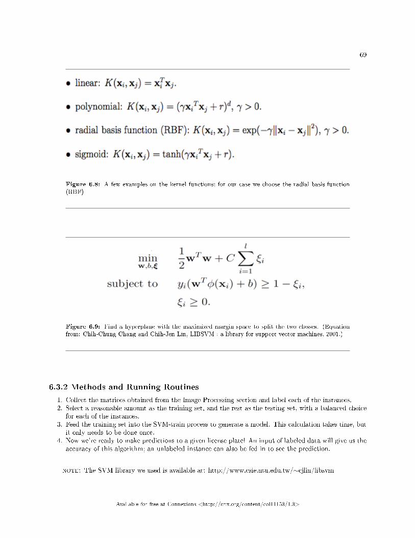
69
Figure 6.8: A few examples on the kernel functions; for our case we choose the radial basis function(RBF)
Figure 6.9: Find a hyperplane with the maximized margin space to split the two classes. (Equationfrom: Chih-Chung Chang and Chih-Jen Lin, LIBSVM : a library for support vector machines, 2001.)
6.3.2 Methods and Running Routines
1. Collect the matrices obtained from the Image Processing section and label each of the instances.2. Select a reasonable amount as the training set, and the rest as the testing set, with a balanced choice
for each of the instances.3. Feed the training set into the SVM-train process to generate a model. This calculation takes time, but
it only needs to be done once.4. Now we're ready to make predictions to a given license plate! An input of labeled data will give us the
accuracy of this algorithm; an unlabeled instance can also be fed in to see the prediction.
note: The SVM library we used is available at: http://www.csie.ntu.edu.tw/∼cjlin/libsvm
Available for free at Connexions <http://cnx.org/content/col11153/1.3>

70 CHAPTER 6. LICENSE PLATE EXTRACTION
6.4 Conclusions4
6.4.1 Results
We were able to successfully locate the license plate in about 70% of our sample pictures, and of the characterswe extracted, we were able to recognize them with about 72.7% accuracy (619 sets of training data).
6.4.2 Future Improvements
6.4.2.1 Compression and Cropping
Since we were targeting Texas plates, which only have red, blue, and white colors, we were able to black outmany parts of the images by wiping out all green regions. In the future, however, we would like to be ableto recognize plates not from Texas that might have green components. Therefore, we should �nd a criteriafor �nding the plates other than color.
6.4.2.2 Letter Recognition
Acquiring State Pattern and Convention AttributesIn many license plates, it is di�cult to tell the di�erence between a zero and an O, even for a human.Therefore, for the purposes of this project, zeros and Os were considered the same. However, in many states,it is actually possible to tell the di�erence because the license plate has a set pattern (e.g., 2 letters, 2numbers, 2 letters). In the future, we could identify what state the plate comes from and then make use ofthis knowledge to get more accuracy in letter recognition.Multi-class Support Vector MachineIn addition, one of the characteristics of SVM is that is solves a two-class problem. In order to get aroundthis, for our project, we used a one-against-the-rest approach. This meant that we basically used the SVMmachine to answer the question, "Is this a __?" 35 (A-Z, 1-9) times for each unknown letter/digit. In thefuture, we will want to look at more e�cient and accurate methods. One of the possible improvement canbe found in the work by T.-K. Huang, R. C. Weng, and C.-J. Lin. Generalized Bradley-Terry Models andMulti-class Probability Estimates. Journal of Machine Learning Research5
Automated Training Set Generation and Extraction E�ciencyFinally, currently, any digit that we feed into the SVM will register as something; we have no way of tellingwhether the image is in fact a letter/digit. In the future, we would like to train the machine to be able totell characters from non-characters. This will allow less rigorous (and time-consuming) computation in theimage-processing section and give our algorithm greater �exibility.
6.4.3 References
Chih-Chung Chang and Chih-Jen Lin, LIBSVM : a library for support vector machines, 2001. Softwareavailable at http://www.csie.ntu.edu.tw/∼cjlin/libsvm6
6.4.4 Special Thanks
Thanks to:
• Dr. Aswin Sankaranarayanan, our mentor• Dr. Richard Baraniuk, the ELEC 301 instructor• Dr. Fatih Porikli (MERL), for providing us with a license plate dataset• Drew Bryant and Brian Bue for technical advising
4This content is available online at <http://cnx.org/content/m33160/1.3/>.5http://www.csie.ntu.edu.tw/∼cjlin/libsvmtools/#96http://www.csie.ntu.edu.tw/∼cjlin/libsvm
Available for free at Connexions <http://cnx.org/content/col11153/1.3>

Chapter 7
An evaluation of several ECG analysis
Algorithms for a low-cost portable ECG
detector
7.1 Introduction1
IntroductionMeasuring vital signs is a crucial part of health care in hospitals across the world. However, these
systems are often extremely expensive, and can often only be given to patients already in intensive care.Upon entering the Emergency ward, however, a patient often needs to wait before receiving direct medicalattention, since it is important for health care professionals to prioritize to whom they direct attention. If alow-cost system of constant monitoring of vital signs existed, the emergency wards could potentially providesimple vital sign monitoring for every patient that entered the hospital, assisting in resource managementand providing better tools with which to evaluate patients [1]. We aim in this module to discuss the basicphysiology behind the ECG trace, provide an overview of the primary signal processing methods used todevelop a heart rate calculator, and describe a test bed that can be used to test an algorithm, with somedemo results. We will end with a discussion on the possibilities these algorithms provide for implementationof a real-time heart rate monitor.
The most important vital sign that can be monitored is the heart rate. Many physiological conditions canbe diagnosed by analyzing heart rate abnormality, and abnormal heart rate has been shown to be a leadingindicator for heart attack[2]. The primary conditions that are diagnosed are bradycardia and tachycardia.Bradycardia is known as the slowing of the heart rate; for adults, below 60 bpm. Tachycardia is the abnormalquickening of the heart; for adults, above 100 bpm.
Tachycardia has been shown to indicate greater oxygen demand for the heart, and eventually, can leadto a heart attack. More speci�cally, the case of ventricular tachycardia
is known to be a potentially life-threatening condition that can lead to sudden death if not immediatelydetected and treated.
Bradycardia also takes on di�erent forms. Sinus bradycardia is a particularly slow heartrate that isassociated with heart diseases. It is also possible for sinus bradycardia not to indicate any medical conditionwhatsoever, such as a patient's good �tness. An alternate form of bradycardia known as Sick sinus syndromeis caused by complications with the sinoatrial node, which naturally monitors the heart. Heart block is themost serious complication, as it can arise suddenly and lead to sudden cardiac arrest or other medicalemergency [3].
1This content is available online at <http://cnx.org/content/m33167/1.3/>.
Available for free at Connexions <http://cnx.org/content/col11153/1.3>
71
72CHAPTER 7. AN EVALUATION OF SEVERAL ECG ANALYSIS
ALGORITHMS FOR A LOW-COST PORTABLE ECG DETECTOR
The primary action that needs to be taken in order to monitor these potentially life-threatening conditionsis to take an ECG (electrocardiogram) recording of the signal. The Electrocardiogram has been extensivelyresearched in the literature, and is relied upon and accepted by many medical professionals as the bestway to measure and diagnose abnormal rhythms of the heart. An ECG machine works by measuring theelectrical activity of the heart over time using electrodes placed at key places of the body. The electricpotential between two electrodes is termed a lead, and averages are taken of di�erent leads around the bodyto determine the overall electrical activity through di�erent axes of the body. The current gold standard isthe 12-lead ECG.
Even though the standard ECG is relied upon as the primary means of diagnosing abnormal rhythms,to actually glean this information o� of the reading of the trace paper requires a great deal of training andspecialization. Unless the trained specialist is present to continuously evaluate every patient's
ECG recording, in an emergency situation a medical complication may go unnoticed.
7.2 How ECG Signals Are Analyzed2
How ECG Signals Are Analyzed :Methods have been developed to analyze the heart rate automatically, by reading the ECG signal trace
and performing certain types of signal processing in order to extract the heart rate information. In analyzingthe ECG, the most important parameter to focus on is the QRS complex. The ECG signal is split up in theliterature into di�erent waves, each with its own nomenclature.
Figure 7.1
2This content is available online at <http://cnx.org/content/m33166/1.2/>.
Available for free at Connexions <http://cnx.org/content/col11153/1.3>

73
Figure 7.2
The QRS complex stands for the key portion of the ECG wave that involves the depolarization of the rightand left ventricles. The QRS complex thus contains the peak of the pulse, and indicates that a heartbeathas occurred.
QRS detection is the most important parameter in the determination of heart rate variability []. Althoughnot every QRS complex contains three separate Q, R and S waves, any conventional combination of thesecan be considered a QRS complex. However, in order to understand the ECG reading and analyze it, it isnecessary to label each part of the complex. Once they are identi�ed, they can be employed to characterizeheartbeats.
Once the QRS has been detected, the location of the QRS in time can be annotated as a beat, and asequence of beat annotation over time can be charted. A heart rate algorithm that takes the sequence ofbeat annotations, measures the time di�erence between beats to calculate a heart rate at every moment intime can then analyze this sequence of beat annotations.
Available for free at Connexions <http://cnx.org/content/col11153/1.3>

74CHAPTER 7. AN EVALUATION OF SEVERAL ECG ANALYSIS
ALGORITHMS FOR A LOW-COST PORTABLE ECG DETECTOR
Figure 7.3
Now, with the necessary heart rate information extracted, basic thresholds can be put on a heart ratevariability system in order to determine if the patient has exited a normal state. If the heart rate is below60 bpm or above 100 bpm for a normal adult, an alarm can be raised to alert the medical personnel thatthe patient requires particular attention.
7.3 Algorithms3
There are a range of available algorithms for QRS detection, based on various methods such as peak detection,slope transform analysis, and length transform analysis. Most of these algorithms involve the use of adaptive�lters, and others use non-adaptive �lters. Adaptive �lters are preferred when it comes to heart rate analysis,largely because ECG signals are non-linear. For this reason, it is necessary to periodically analyze the outputand modify the �lter parameters accordingly.
We aim in this project to give a brief overview of the existing literature and algorithms, and comparethe robustness of two leading QRS detection algorithms in accurately detecting heartbeats.
Algorithms for ECG AnalysisThere is an extensive library of QRS detection algorithms available in the medical literature, since QRS
detectors are the most important signal processing algorithm involved in ECG analysis. We will here analyzethree primary algorithm methods: Peak Detections, Slope transform analysis, and length transform analysis.
Particular Peak Detection AlgorithmThe peak detection algorithm that we chose to analyze speci�cally looks at a 160ms window, splits the
window into three segments, and �nds if the maximum value is contained within the center segment; if so, abeat is annotated. If no beat is detected for longer than 200ms, the threshold is updated using an adaptive�lter that functions according to the rate described below:
3This content is available online at <http://cnx.org/content/m33164/1.2/>.
Available for free at Connexions <http://cnx.org/content/col11153/1.3>
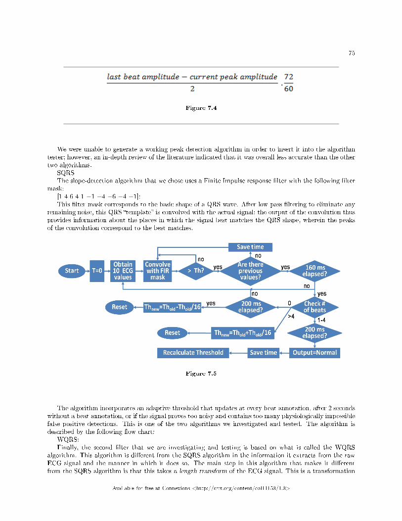
75
Figure 7.4
We were unable to generate a working peak detection algorithm in order to insert it into the algorithmtester; however, an in-depth review of the literature indicated that it was overall less accurate than the othertwo algorithms.
SQRSThe slope-detection algorithm that we chose uses a Finite Impulse response �lter with the following �lter
mask:[1 4 6 4 1 −1 −4 −6 −4 −1];This �lter mask corresponds to the basic shape of a QRS wave. After low-pass �ltering to eliminate any
remaining noise, this QRS �template� is convolved with the actual signal; the output of the convolution thusprovides information about the places in which the signal best matches the QRS shape, wherein the peaksof the convolution correspond to the best matches.
Figure 7.5
The algorithm incorporates an adaptive threshold that updates at every beat annotation, after 2 secondswithout a beat annotation, or if the signal proves too noisy and contains too many physiologically impossiblefalse positive detections. This is one of the two algorithms we investigated and tested. The algorithm isdescribed by the following �ow chart:
WQRS:Finally, the second �lter that we are investigating and testing is based on what is called the WQRS
algorithm. This algorithm is di�erent from the SQRS algorithm in the information it extracts from the rawECG signal and the manner in which it does so. The main step in this algorithm that makes it di�erentfrom the SQRS algorithm is that this takes a length transform of the ECG signal. This is a transformation
Available for free at Connexions <http://cnx.org/content/col11153/1.3>
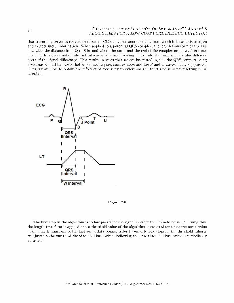
76CHAPTER 7. AN EVALUATION OF SEVERAL ECG ANALYSIS
ALGORITHMS FOR A LOW-COST PORTABLE ECG DETECTOR
that essentially serves to convert the erratic ECG signal into another signal from which it is easier to analyzeand extract useful information. When applied to a potential QRS complex, the length transform can tell ushow wide the distance from Q to S is, and where the onset and the end of the complex are located in time.The length transformation also introduces a non-linear scaling factor into the mix, which scales di�erentparts of the signal di�erently. This results in areas that we are interested in, i.e. the QRS complex beingaccentuated, and the areas that we do not require, such as noise and the P and T waves, being suppressed.Thus, we are able to obtain the information necessary to determine the heart rate whilst not letting noiseinterfere.
Figure 7.6
The �rst step in the algorithm is to low pass �lter the signal in order to eliminate noise. Following this,the length transform is applied and a threshold value of the algorithm is set as three times the mean valueof the length transform of the �rst set of data points. After 10 seconds have elapsed, the threshold value isreadjusted to be one-third the threshold base value. Following this, the threshold base value is periodicallyadjusted.
Available for free at Connexions <http://cnx.org/content/col11153/1.3>

77
Figure 7.7
Once the algorithm detects a potential QRS complex in which the length of QS has just exceeded thethreshold, the time `t' the event occurred is saved. Then we travel backward for 125 ms to the minimumvalue of the length Lmin and forward for 125 ms from `t' to obtain the maximum value Lmax, where L isthe magnitude of the length transform. Next, we again travel backward to recover where the QRS onset islocated in time and forward to recover where the end is located in time. The onset and end times are addedwith -20ms and +20ms respectively, in order to provide for potential losses caused by the threshold. Thisadjustment is based on statistical observations of typical heart rates and ECG signals. Finally, the algorithmwaits for 250ms before proceeding to check for another QRS complex in order to avoid detecting the samebeat again by mistake.
7.4 Testing4
Test-bedA test bed can be setup using C. The data set used for testing in this module was a subset of the MIT-
BIH Noise Stress test available online at www.physionet.org5 . To evaluate sensitivity to noise, one can readdi�erent noise level recordings; here, we analyze three in particular from the Physionet Noise Stress Testtool, selecting 3 di�erent Signal to Noise Ratios (SNR): 24 dB, 18 dB, and 0 dB.
First, download all of the compilers and specialized libraries for gathering ECG data, initialize storagespaces, processing signals stored in a certain format, formatting outputs for consistency and re-use in otheralgorithms, etc. This is all contained in the WFDB library toolkit. Then, download a speci�c heart rate �leof your choice from the Physionet database and run one of the C programs containing one of the availablealgorithms under the physiological signal processing header. These algorithms are designed to output aPhysionet-compatible annotation �le. This annotation �le can then be processed manually by running theinstantaneous heart rate algorithm (ihr). Using this setup also allows one to save the output of the algorithmas a regular annotation �le. This ensures that in the future, the setup could be used to read annotation �lesand save them directly onto a memory storage unit for processing elsewhere.
The test here constructed consists of running each one of the three algorithms on 3 di�erent data �lesfrom the noise stress test. The annotations are compared to reference annotations available on the Physionet-website. Using Physionet's �bxb� program, one can compare the annotations beat by beat. The bxb program
4This content is available online at <http://cnx.org/content/m33168/1.2/>.5http://www.ncbi.nlm.nih.gov/pmc/articles/PMC1560458/www.physionet.org
Available for free at Connexions <http://cnx.org/content/col11153/1.3>

78CHAPTER 7. AN EVALUATION OF SEVERAL ECG ANALYSIS
ALGORITHMS FOR A LOW-COST PORTABLE ECG DETECTOR
outputs the two key parameters of interest in the analysis of heart beat detection: Sensitivity and PositivePredictivity.
Sensitivity (Se) = TP/(TP+MB)Positive Predictivity (+P) = TP/(TP+FP)TP: number of true positive detections.MB: number of false negatives or missed beatsFP: number of false positives; the system detected a beat where the reference annotation showed no beat.ResultsTable 1
Noisy Signal with0dB SNR
Noisy Signal with18dB SNR
Noisy Signal with24dB SNR
Non-Noisy Signal
SQRS WQRS SQRS WQRS SQRS WQRS SQRS WQRS
QRSSensitiv-ity:
54.91% 99.53% 92.80% 100.00% 97.70% 100.00% 96.55% 99.97%
QRSPositivePredic-tivity:
77.75% 57.68% 95.18% 98.46% 98.63% 99.64% 99.76% 99.27%
Table 7.1
As can be seen from Table 1, the WQRS algorithm is overall more robust and tolerant to noise thanthe SQRS algorithm, particularly in the Sensitivity ratio. To note, however, is the situation that occurs toWQRS at 0dB noise, wherein the SQRS actually obtains a better Positive Predictivity ratio. This indicatesthat the WQRS formula is particularly adept at correctly noting beats and rarely misses beats, but is lesscapable of avoiding false positives at high noise levels. However, the WQRS also suppresses information inthe ECG signal that we do not need i.e. the P and T waves which also lends to the �lters e�ectiveness. Giventhat the overall spread from the other noise levels favors WQRS more, it seems best to side with WQRS formost applications.
7.5 Conclusion6
ConclusionWe have thus shown in this module an overview of the large body of established research in signal
processing from which to draw from in developing a functional QRS detector and heart rate analyzer. Theopen-source community has developed a robust set of algorithms from which to streamline algorithm testingand implementation. We have conclusively demonstrated that the algorithms developed are capable of noisetolerance to an acceptable medical standard, with high sensitivity ratio and high Positive Predictivity ratio.
In particular, we found the WQRS algorithm was the most consistently noise-tolerant, and most accurateat all noise levels, and we recommend its use in implementation trials.
Given the open-source nature of the programs here analyzed, the reader is encouraged to download thetoolkit and run the programs themselves to verify the conclusions of this module.
Having completed this testing, it is clear that this capable testbed available from the MIT Physiotoolkitdatabase would allow a team to implement readily the software onto a processing program for real-time.
The particular steps that a team needs to take in order to implement this algorithm are to modify it forreal-time signal analysis by attaching a set of electrodes to the patient, creating a set of analog �lters to
6This content is available online at <http://cnx.org/content/m33165/1.2/>.
Available for free at Connexions <http://cnx.org/content/col11153/1.3>

79
remove noise, and programming a data bu�er from which to read in analog voltage signals from electrodesand separate them into discrete components that an Analog to Digital Converter can sample and read intoa digital processor. These are topics out of the scope of this module.
Available for free at Connexions <http://cnx.org/content/col11153/1.3>

80CHAPTER 7. AN EVALUATION OF SEVERAL ECG ANALYSIS
ALGORITHMS FOR A LOW-COST PORTABLE ECG DETECTOR
Available for free at Connexions <http://cnx.org/content/col11153/1.3>

Chapter 8
Sparse Signal Recovery in the Presence
of Noise
8.1 Introduction1
8.1.1 Introduction
As we progress into the era of information overload, it becomes increasingly important to �nd ways toextract information e�ciently from data sets. One of the key concerns in signal processing is the accuratedecoding and interpretation of an input in a minimal period of time. In the distant past, the informationtheorists' objective primarily involved reducing the signal elements to be processed. Now, with a multitudeof extraction options, we are also concerned about the computation time required to interpret each element.
In this project, we investigate a few methods by which we can �accurately� reconstruct an arbitrarilycomplex signal using a minimum number of iterations. The input signals we probe are deemed sparse �that is, they are constructed using a number of basis vectors that is small relative to the length of the signal.This generally means that the signals consist mostly of zero values, with spikes at a few selected positions.We compare the signal-to-noise ratios achieved by our recovery methods after speci�ed numbers of iterationsupon a variety of input signals, and deduce a few conclusions about the most e�cient and most feasiblerecovery methods.
8.2 Theory2
8.2.1 Theory
8.2.1.1 Motivation
In theory, we should never have to 'recover' a signal � it should merely pass from one location to another,undisturbed. However, all real-world signals pass through the infamous �channel� � a path between thetransmitter and the receiver that includes a variety of hazards, including attenuation, phase shift, and,perhaps most insidiously, noise. Nonetheless, we depend upon precise signal transmission daily � in ourwatches, computer networks, and advanced defense systems. Therefore, the �eld of signal processing concernsitself not only with the deployment of a signal, but also with its recovery in the most e�cient and mostaccurate manner.
1This content is available online at <http://cnx.org/content/m33082/1.2/>.2This content is available online at <http://cnx.org/content/m33087/1.2/>.
Available for free at Connexions <http://cnx.org/content/col11153/1.3>
81

82 CHAPTER 8. SPARSE SIGNAL RECOVERY IN THE PRESENCE OF NOISE
8.2.1.2 Types of Noise
Noise takes many forms. The various 'colors' of noise are used to refer to the di�erent power spectral densitycurves that types of noise exhibit. For example, the power density of pink noise falls o� at 10dB per decade.The power density spectrum of pink noise is �at in logarithmic space. The most common type of noise,however, is white noise. White noise exhibits a �at power density spectrum in linear space. In manyphysical process (and in this report), we deal primarily with Additive White Gaussian Noise � abbreviatedAWGN. As a reminder, the Gaussian distribution has the following PDF (Probability Density Function):
Figure 8.1
µ is the mean; σ2 ≥ 0 is the variance.
8.2.1.3 Sparse Signals
An additional constraint we imposed upon our input signals was that they were required to be sparse. Asignal that is sparse in a given basis can be reconstructed using a small number of the basis vectors in thatbasis. In the standard basis for Rn, for example, the signal (1,0,0,0,...,0) would be as sparse as possible � itrequires only the basis vector e1 for reconstruction (in fact, e1 is the signal!). By assuming that the originalsignals are sparse, we are able to employ novel recovery methods and minimize computation time.
8.2.1.4 Typical Reconstruction Approaches
We have a number of choices for the recovery of sparse signals. As a �rst idea, we could �optimally select�the samples we use for our calculations from the signal. However, this is a complicated and not alwaysfruitful process.
Another approach is Orthogonal Matching Pursuit (OMP). OMP essentially involves projecting alength-n signal into the space determined by the span of a k-component �nearly orthonormal� basis (a randomarray of 1/sqrt(n) and (-1)/sqrt(n) values). Such a projection is termed a Random Fourier Projection.Entries in the projection that do not reach a certain threshold are assigned a value of zero. This computationis iterated and the result obtained is an approximation of the original sparse signal. Unfortunately, OMPitself can be fairly complicated, as the optimal basis is often a wavelet basis. Wavelets are frequency �packets�- that is, localized in both time and frequency; in contrast, the Fourier transform is only localized in frequency.
8.2.1.5 Signal Reconstruction: Our Method
The fundamental principle for our method of signal analysis is determining where the signal is not, ratherthan �nding where it is. This information is stored in a mask that, when multiplied with the runningaverage of the signal, will provide the current approximation of the signal. This mask is built up bydetermining whether a given value in the signal is above a threshold, which is determined by the standarddeviation of the noise; if so, the value is most likely a signal element. This process is repeated until thesignal expected is approximately equal to a signal stored in a library on the device. While this operation isnaturally more noticeable at each iteration with sparse signals, even for non-sparse signals the only limiting
Available for free at Connexions <http://cnx.org/content/col11153/1.3>

83
factor is the minimum value of the signal. For reasons of application, the primary limiting factor is thenumber of samples required to recover the signal. This is because the raw mathematical operations takefractions of a second to a few seconds to execute (which is more than enough for conventional applications).The signal itself may be transmitted for a very short period; the requisite number of samples must begarnered before transmission halts. Further, given an arbitrary amount of computation time, our algorithmcan reconstruct a sparse signal contaminated with any level of AWGN � there is no mathematical limit onthe recovery process. This is an impressive and surprising feat.
8.3 Implementation3
8.3.1 Implementation
Our implementation of the system was based around a controller program, which accepts the password tobe transmitted, and then simulate the transmission and reconstruction. The program then returns whetheror not the password received is the same as that which activated the system. In the �nal application, thecontroller is called repeatedly until the system is activated; it returns immediately after a non-match, andcontinues in sequence after the �rst element is matched.
For each of the passwords element's iterations in the controller the following algorithm is used. Thethreshold is set to [the minimum value of the ideal signal minus three times the standard deviation of thebase noise] (in our case one), and the mask is initialized to all ones. Then we prime the noise to reach eitherthat standard deviation or less by priming the running total with a series of samples, the exact number ofwhich is determined by the standard deviation of the noise. Then we execute the following function untileither it runs a set number of times, or succeeds. Then the program compares the reconstructed signal afterthe iteration with the ideal signals, and returns if there is a reasonable match.
This function does the following four times: it samples the signal, updates the running total, and countswhether the maximum imaginary or real part of the Fourier transform of the signal is greater than thethreshold. If at least two of the four cycles result in a value greater than the threshold, the mask's valueat that point is set to the previous value of the mask; otherwise, the mask's value is set to zero. Thisallows a degree of leniency (which is useful in an inherently probabilistic method) and drastically reducesthe probability of failure, albeit at the expense of increasing processing time.
The priming of the noise either reduces it to a standard deviation of two and a half, or three, based onthe standard deviation of the noise. The method which is selected will result in fewer net samples requiredthan the alternative method: although processing the information can take large quantities of samples, pre-processing requires sd^2/(2.5^2) or sd^2/(3^2) samples; hence, a larger denominator can cut o� incrediblequantities of samples. The reason why these values in particular were selected is that experimentally wedetermined that at 2.5 standard deviations, most signals required only one additional sample to become fullyreconstructed, while at 3 standard deviations, they took a couple dozen to a few hundred, and a maximumof a few thousand additional samples, but it appeared to terminate the vast majority of the time as shownin Figure 1 and Figure 2.
3This content is available online at <http://cnx.org/content/m33081/1.2/>.
Available for free at Connexions <http://cnx.org/content/col11153/1.3>
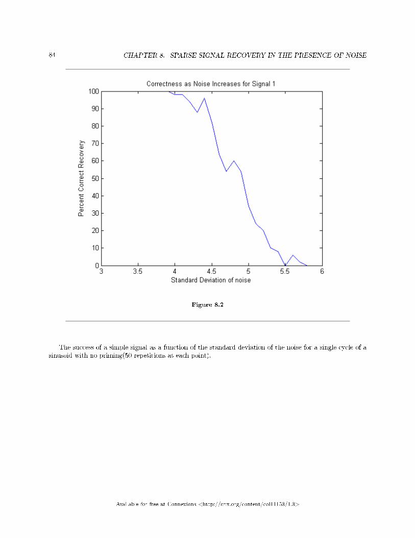
84 CHAPTER 8. SPARSE SIGNAL RECOVERY IN THE PRESENCE OF NOISE
Figure 8.2
The success of a simple signal as a function of the standard deviation of the noise for a single cycle of asinusoid with no priming(50 repetitions at each point).
Available for free at Connexions <http://cnx.org/content/col11153/1.3>

85
Figure 8.3
The success of a sum of a frequency one sine wave, a frequency four sine wave, and a frequency 20 cosinewave as a function of the standard deviation of the noise with no priming(50 repetitions at each point).
The priming is a necessity, since without it, the probability of success decreases rapidly as the standarddeviation increases, but with it the probability of success, while not one, remains constantly above 99%.This is because after priming the e�ective standard deviation is always three or less, making the originalsignal consistently recoverable.
8.3.2 Timing Analysis
All of the initializitions before the priming, assignations etc. require O(1) operations. The priming itselfrequires O(sd^2) operations. The post priming processing, requires O(library size) operations since althoughthe �t is O(N*logN), N is bounded and therefore even if the sd wasn't bounded to minimize the computationit still would always be less than a constant value. The only variable processing part is the comparisons withthe library, which is O(libsize*N*logN) with N being bounded, simplifying to O(libsize). This means thatthe algorithm itself is O(sd^2)+O(libsize)=O(sd^2) since libsize will tend to be small. This is supported byexperimental results as shown in Figure 1 and Figure 2.
Available for free at Connexions <http://cnx.org/content/col11153/1.3>
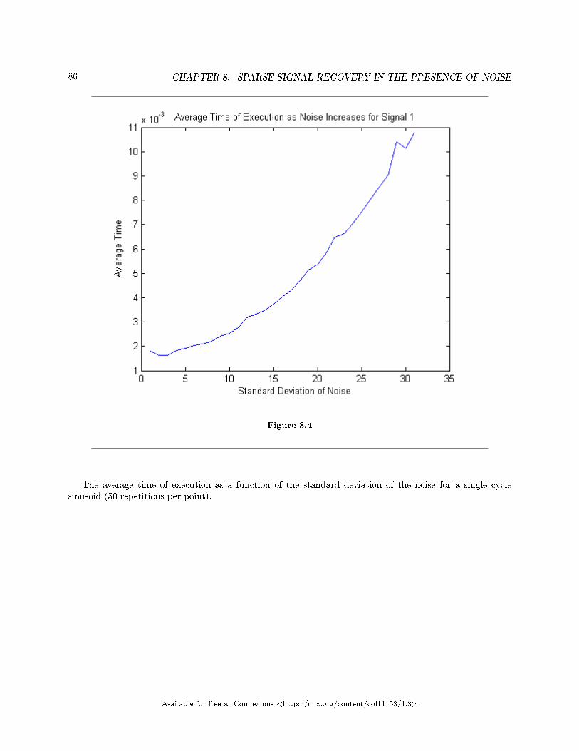
86 CHAPTER 8. SPARSE SIGNAL RECOVERY IN THE PRESENCE OF NOISE
Figure 8.4
The average time of execution as a function of the standard deviation of the noise for a single cyclesinusoid (50 repetitions per point).
Available for free at Connexions <http://cnx.org/content/col11153/1.3>

87
Figure 8.5
The average time of execution as a function of the standard deviation of the noise for the sum of afrequency 1, sine wave, a frequency 4 sine wave, and a frequency 20 cosine wave (50 repetitions per point).
For a real world application, it is also important to know not only the time it takes to execute theentire program, but also the number of samples that are required in order to reconstruct the signal. This isbecause the signal will only be transmitted for a limited time, so the hardware must be able to take the rightnumber of samples in that time. From the processing perspective, even with very slow hardware the signalcould eventually be reconstructed, but the same is not the case if the correct number of samples cannotbe garnered. The number of samples required is always on O(sd^2) speci�cally sd^2/6.25+1 if sd<76, andsd^2/9+∼200 if sd>=76. The experimental values are shown in Figure 3 and Figure 4.
Available for free at Connexions <http://cnx.org/content/col11153/1.3>

88 CHAPTER 8. SPARSE SIGNAL RECOVERY IN THE PRESENCE OF NOISE
Figure 8.6
The average number of samples required to reconstruct the signal as standard deviation increases for asingle cycle sine wave (50 repetitions at each point).
Available for free at Connexions <http://cnx.org/content/col11153/1.3>

89
Figure 8.7
The average number of samples to reconstruct the signal as a function of the standard deviation of thenoise for the sum of a frequency 1 sine wave, a frequency 4 sine wave, and a frequency 20 cosine wave (50repetitions per point).
8.3.3 Examples of Execution
All of the following �gures are comprised of a series of graphs. The �rst graph is the initial signal with noise,as well as the initial signal; the next four graphs are the reconstructed signal at consecutive iterations alongwith the initial signal; the �nal graph is the �nal reconstructed signal along with the initial signal.
Available for free at Connexions <http://cnx.org/content/col11153/1.3>
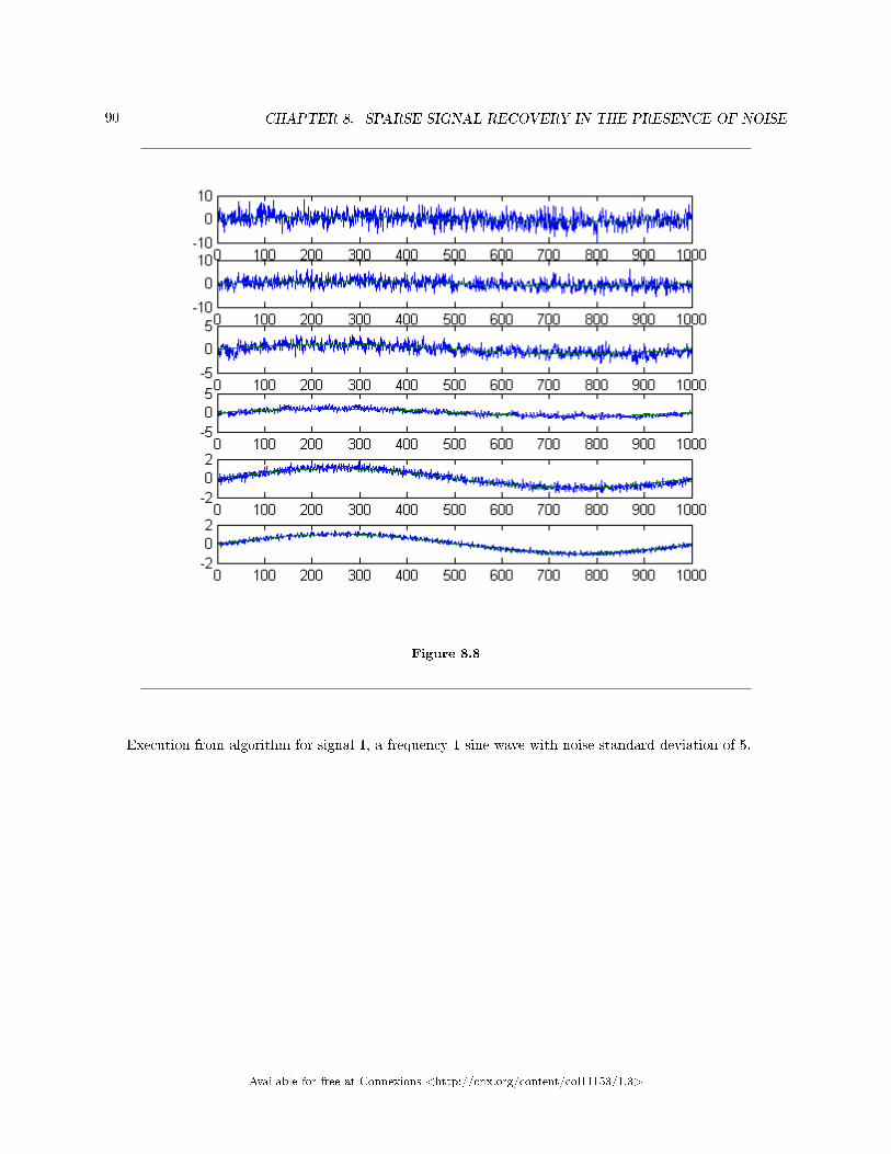
90 CHAPTER 8. SPARSE SIGNAL RECOVERY IN THE PRESENCE OF NOISE
Figure 8.8
Execution from algorithm for signal 1, a frequency 1 sine wave with noise standard deviation of 5.
Available for free at Connexions <http://cnx.org/content/col11153/1.3>

91
Figure 8.9
Execution from algorithm for signal 10, a frequency 10 cosine wave with noise standard deviation of 5.
Available for free at Connexions <http://cnx.org/content/col11153/1.3>

92 CHAPTER 8. SPARSE SIGNAL RECOVERY IN THE PRESENCE OF NOISE
Figure 8.10
Execution from algorithm for signal 13, the sum of a frequency 1 sine wave, a frequency 4 sine wave, anda frequency 20 cosine wave with noise standard deviation of 5.
8.4 Conclusion4
8.4.1 Conclusion
With priming, the regression line correlating number of samples and standard deviation is roughly(sd^2)/6.5 + 1, which amounts to O(N^2) complexity. However, although this may seem slow, our methodpermits perfect recovery of complicated (albeit sparse) signals with arbitrary levels of AWGN. Thus, forreasonable data set sizes and values of standard deviation, the algorithm functions quite nicely for accuratesignal reconstruction. Although if given in�nite samples and time, it can recover any signal that is relativelysparse given in�nite time.
Without priming the noise, and taking 50 samples, we can achieve O(1) complexity � extremelydesirable, but the recovery percentage falls o� rapidly with increase in noise standard deviation starting atstandard deviation values around 3.5. Thus, this version of the algorithm could be desirable in non-critical
4This content is available online at <http://cnx.org/content/m33080/1.2/>.
Available for free at Connexions <http://cnx.org/content/col11153/1.3>

93
applications where the strength of the noise is known to be low relative to that of the signal. We certainlywould not recommend using the non-primed algorithm in data sensitive digital applications.
8.4.2 Further Avenues of Inquiry
Colored NoiseIt would be interesting to extend the algorithm to accept di�erent types of noise � pink, brown, purple, etc.Logically the exact same algorithm would work on these, but it would be nice to verify this experimentally.Physical PrototypeA physical prototype of this system would allow a far better testing of the theory than simple simulation.Unfortunately, due to the cost of even moderate quality receivers and FPGAs, this was not feasible.Dynamic NoiseOne major bene�t of a noise resistant system is ECCM, Electronic Counter Countermeasures (counter-jamming). It would be interesting to test whether a system using the described algorithm could resist noisefrom a transmitter moving towards the system (without simply taking a conservative estimate of worst-casenoise during the signal reconstruction period).Dynamic PrimingA useful addition to this algorithm, would be to be able to pick the optimal bound for priming to minimizethe number of samples rather than simply choosing the best of two options.
8.5 Code5
8.5.1 Code
The following is the MATLAB source code for each of the components of our project.
8.5.1.1 addNoise.m
function out = addNoise(sig,mean,sd,Plot)
%addNoise
%adds noise with given mean and sd to the signal
rand=randn(1,1000)*sd+mean;
out=sig+rand;
if(Plot==1)
plot(1:1000,out,1:1000,sig);
end
end
8.5.1.2 sample.m
function out = sample(sd,plot,sig)
%sample
%samples a manually constructed signal, and adds gaussian noise to it
%with a standard deviation that is provided
out=fft(addNoise(sig,0,sd,plot));
end
5This content is available online at <http://cnx.org/content/m33079/1.2/>.
Available for free at Connexions <http://cnx.org/content/col11153/1.3>

94 CHAPTER 8. SPARSE SIGNAL RECOVERY IN THE PRESENCE OF NOISE
8.5.1.3 init.m
function [out,samp]=init(sig,sd)
%averages the signal and the noise over a number of samples to make the
%noise level manageable
out=sig+randn(1,1000).*sd;
%optimize number of samples
if sd<76val=6.25;
else
val=9;
end
samp=floor((ceil(sd))^2/(val));
for n=2:samp
out=(out.*(n-1)+sig+randn(1,1000).*sd)/n;
end
out=fft(out);
end
8.5.1.4 simpleIterate.m
function [mask, NSig,runT] = simpleIterate(sigMask,threshold,run,n,sd,sig)
%simpleIterate(sigMask,threshold,run,n)
%computes an iteration of the thresholding, with a running average of run,
%on iteration n, with the current signal mask of sigMask
%returns the new signal mask, the current signal(non-masked) NSig and the
%running average of the signal runT
siz=size(sigMask);
temp=zeros(1,siz(2));
for i=1:4
NSig=sample(sd,0,sig).*sigMask;
if(n==1)
runT=NSig;
else
runT=(run.*(n-1)+NSig)/n;
end
%temp=temp+(max(abs(real(NSig)),abs(imag(NSig)))>threshold);temp=temp+(max(abs(real(runT)),abs(imag(runT)))>threshold);%temp=temp+(abs(NSig)>threshold);
end
mask=zeros(1,siz(2));
for l=1:siz(2)
if(temp(l)<2)mask(l)=0;
else
mask(l)=sigMask(l);
end
end
end
Available for free at Connexions <http://cnx.org/content/col11153/1.3>

95
8.5.1.5 testArbitary.m
function [flag,samples,time]=testArbitrary(sig,sd)
%Simulates the transmission of a signal in the library, and tests whether
%or not it can be recovered.
siglib=cat(1,sin(0:pi/500:(1000*pi-1)/500),sin(0:pi/250:(2000*pi-1)/500),sin(0:pi/125:(4000*pi-1)/500),sin(0:pi/50:(10000*pi-1)/500),sin(0:pi/25:(20000*pi-1)/500));
siglib=cat(1,siglib,sin(0:pi/500:(1000*pi-1)/500)+sin(0:pi/50:(10000*pi-1)/500),cos(0:pi/500:(1000*pi-1)/500),cos(0:pi/250:(2000*pi-1)/500),cos(0:pi/125:(4000*pi-1)/500),cos(0:pi/50:(10000*pi-1)/500));
siglib=cat(1,siglib,cos(0:pi/25:(20000*pi-1)/500),cos(0:pi/25:(20000*pi-1)/500)+sin(0:pi/500:(1000*pi-1)/500),sin(0:pi/500:(1000*pi-1)/500)+sin(0:pi/125:(4000*pi-1)/500)+cos(0:pi/25:(20000*pi-1)/500));
sigmax=max(abs(fft(siglib(sig,:))));
threshhold=sigmax-3*max(abs(real(fft(randn(1,1000)))));
tolerance=.5;
A=ones(1,1000);
flag=0;
tic
[C,samples]=init(siglib(sig,:),sd);
for i=1:10000
[A,B,C]=simpleIterate(A,threshhold,C,i+samples,sd,siglib(sig,:));
for j=1:size(siglib)
if(abs(ifft(A.*C)-siglib(j,:))<tolerance)flag=j;
break;
end
end
if(flag>0)break;
end
end
samples=samples+i;
time=toc;
end
8.5.1.6 Controller.m
function accepted = Controller(enteredpassword,sd)
%Tests whether or not a transmission of a password will activate the system
%This simulates the noise and processing as well as the values
actualpassword=cat(1,13,5,10,4,2,8);
accepted=1;
redundancy=3;
for i=1:size(actualpassword);
flag=0;
%while flag==0
for j=1:redundancy
[flag,runs]=testArbitrary(enteredpassword(i),sd);
end
if(flag∼=actualpassword(i))accepted=-i;
break;
end
end
Available for free at Connexions <http://cnx.org/content/col11153/1.3>

96 CHAPTER 8. SPARSE SIGNAL RECOVERY IN THE PRESENCE OF NOISE
end
8.5.1.7 Controller2.m
function Controller2()
%Helper function used to graph trends
sig=1;
for sd=0:30
passed=0;
for reps=1:50
if(testArbitrary(sig,3+sd/10)==sig)
passed=passed+1;
end
end
temp(sd*10-29)=passed
end
subplot(1,1,1);
plot(temp);
end
8.6 References and Acknowledgements6
8.6.1 References and Acknowledgements
We wish to thank our mentor, JP Slavinsky. Without your guidance and support, this project would nothave been possible.
Many thanks also to Dr. Rich Baraniuk � for creating Connexions, and (arguably more importantly),for presenting inspiring signal processing lectures throughout the semester.
J D Haupt's presentation to the Electrical Engineering department on sparse signal reconstruction wasintegral to the development of our algorithm, although it concentrated on e�ciency rather than arbitraryreconstruction.
The algorithms and techniques discussed in the following papers were used for comparison against ouralgorithm:
Haupt, J. and R. Nowak. "Signal Reconstruction From Noisy Random Pro-jections." IEEE Trans. Info. Theory, vol.52, no.9, pp.4036-4048, 2006.http://ieeexplore.ieee.org/stamp/stamp.jsp?arnumber=1683924&isnumber=354597
J. Tropp and A. Gilbert, "Signal Recovery from Partial Information via Orthogonal Match-ing Pursuit." IEEE Trans. Info. Theory, vol. 53, no. 12, pp. 4655�4666, 2007.http://www.math.lsa.umich.edu/∼annacg/papers/TG05-signal-recovery-rev-v2.pdf8
6This content is available online at <http://cnx.org/content/m33083/1.2/>.7http://ieeexplore.ieee.org/stamp/stamp.jsp?arnumber=1683924&isnumber=354598http://www.math.lsa.umich.edu/∼annacg/papers/TG05-signal-recovery-rev-v2.pdf
Available for free at Connexions <http://cnx.org/content/col11153/1.3>
97
8.7 Team9
8.7.1 Team
8.7.1.1 Grant Cathcart
Figure 8.11
Grant Cathcart was born in Cleveland Ohio, in 1989. Grant is currently a junior Electrical Engineeringmajor at Rice University specializing in signals and systems. Grant is employed by the Navy as part of theTactical Electronic Warfare Division. When not working on projects and cursing matlab, Grant likes to playchess and video games.
9This content is available online at <http://cnx.org/content/m33086/1.2/>.
Available for free at Connexions <http://cnx.org/content/col11153/1.3>

98 CHAPTER 8. SPARSE SIGNAL RECOVERY IN THE PRESENCE OF NOISE
8.7.1.2 Graham de Wit
Figure 8.12
Graham was born in Cincinnati, OH in 1989. However, he spent most of his life in Memphis, TN, the Homeof the Blues. Graham is currently a junior Electrical Engineering major at Rice University specializing inComputer Engineering. Graham enjoys convolving signals, computing Fourier Transforms, and inducingcapacitor explosions. When he is not buried in problem sets, Graham spends time eating, sleeping, hangingout with friends, and composing music via his synthesizers.
Available for free at Connexions <http://cnx.org/content/col11153/1.3>

99
8.7.1.3 Nicholas �Re'Sean� Newton
Figure 8.13
Nicholas Newton was born in Wichita Falls,TX in 1989. He is currently an junior Electrical Engineeringmajor with a specialization in Computer Engineering at Rice University . He plans to attend GraduateSchool after he graduates from Rice. Nicholas has a deep passion for the Computer Engineering industryand computers in general. Outside of his academic career, Nicholas enjoys working out and a number ofdi�erent sports.
Available for free at Connexions <http://cnx.org/content/col11153/1.3>

100 CHAPTER 8. SPARSE SIGNAL RECOVERY IN THE PRESENCE OF NOISE
Available for free at Connexions <http://cnx.org/content/col11153/1.3>

Chapter 9
Video Stabilization
9.1 Introduction1
IntroductionA common problem in dealing with Unmanned Aerial Vehicles (UAVs) is image stabilization. If an operatorwishes to control the craft in real-time, a camera mounted on the UAV is often a good solution. This videofeed, if left in its original state, has varying amounts of jitter, which in turn makes operating the craft moredi�cult and makes the footage of the �ight much less pleasant to watch. We decided that we could stabilizethe video without using any additional hardware-based assistance (such as gyroscopes) with the digitalsignal processing techniques we've learned over the semester. Our �rst approach to solving this problemwas to correlate each video frame with the previous one, but this proved to be less than optimal ; thereexists a faster, more accurate technique. Enter KLT feature tracking and Serial A�ne Transformation. Weused a freely-available KLT feature tracker from Stan Birch�eld, then prototyped our a�ne transformationtechniques in MATLAB. We have started porting our work to C, and in the future we expect this sort ofsolution to be fully implemented on GPUs for real-time processing.
9.2 Background2
BackgroundImage stabilization can be done in many di�erent ways. Kanade-Lucas-Tomasi (KLT) feature tracking3 isone of the computationally inexpensive ways, in comparison to 2-D correlation and even SIFT. We choseStan Birch�eld's implementation because it is written in C and we found it easy to interface to in comparisonwith other open-source implementations.
When we have a set of common features between two images, we can 'undo' the transformation thatmakes the second image's features reside in a di�erent location than the �rst, creating a new image whosefeatures have similar locations to those in the �rst image.
In order to accomplish this, we use a series of least-squares a�ne transformations on the set of features todetermine the `best' values for the un-a�ne we perform to correct the later image. After this, we then �lterthe resulting a�ne transformation, keeping the low-frequency movement (such as panning) and removingthe high-frequency jitter.
Pictorally, the process is as such:
1This content is available online at <http://cnx.org/content/m33246/1.1/>.2This content is available online at <http://cnx.org/content/m33247/1.1/>.3http://en.wikipedia.org/wiki/Kanade-Lucas-Tomasi_Feature_Tracker
Available for free at Connexions <http://cnx.org/content/col11153/1.3>
101

102 CHAPTER 9. VIDEO STABILIZATION
9.3 Procedures4
9.3.1 A�ne Transform Estimation
We wish to approximate the movement of the feature points by an a�ne transform, because it can accountfor rotation, zooming, and panning, all of which are common features in videos. The coordinates of a feature
4This content is available online at <http://cnx.org/content/m33251/1.1/>.
Available for free at Connexions <http://cnx.org/content/col11153/1.3>

103
in the old frame are written as (x0, y0) and in the new frame as (x1, y1). Then an a�ne transform can bewritten as: x1
y1
=
a b
c d
x0
y0
+
e
f
(9.1)
However, this form needs some modi�cation to deal with multiple point pairs at once, and needs rearrangingto �nd a, b, c, d, e, and f . It can be easily veri�ed that the form below is equivalent to the one just given:
x0 y0 0 0 1 0
0 0 x0 y0 0 1
a
b
c
d
e
f
=
x1
y1
(9.2)
With this form, it is easy to add multiple feature points by stacking two additional rows on the left
and on the right. Denoting the pairs of points as((x
(1)0 , y
(1)0
),(x
(1)1 , y
(1)1
)),((x
(2)0 , y
(2)0
),(x
(2)1 , y
(2)1
)),((
x(3)0 , y
(3)0
),(x
(3)1 , y
(3)1
)), etc, the matrices will now look like:
x(1)0 y
(1)0 0 0 1 0
0 0 x(1)0 y
(1)0 0 1
x(2)0 y
(2)0 0 0 1 0
0 0 x(2)0 y
(2)0 0 1
x(3)0 y
(3)0 0 0 1 0
0 0 x(3)0 y
(3)0 0 1
......
......
......
a
b
c
d
e
f
=
x(1)1
y(1)1
x(2)1
y(2)1
x(3)1
y(3)1
...
(9.3)
So long as there are more than three points, the system of equations will be overdetermined. Therefore theobjective is to �nd the solution [a, b, c, d, e, f ] in the least squares sense. This is done using the pseudoinverseof the matrix on the left.
9.3.2 Filtering
The a�ne transforms produced above only relate one video frame to the one immediately after it. Theproblem with this is that if the video is jerky, it will take several consecutive frames to have a good idea ofwhat the average position of the camera is during this time. Then the di�erence between the current locationand the moving-average location can be used to correct the current frame to be in this average position.
When the features are tracked frame-to-frame, it constitutes an implicit di�erentiation in terms of mea-suring the overall movement of the camera. In order to track changes across many frames, we sequentiallyaccumulate the frame-to-frame di�erences. This is akin to an integral operator. Unfortunately, when inte-grating imperfect data, errors will build up linearly in time, and that is true here. However, since the streamof integrated a�ne transforms is not used directly, these errors are not as important.
Once the stream of integrated a�ne transforms is generated, the goal is to undo high-frequency motions,while leaving the low-frequency motions intact. This is done by treating the coe�cients of the streamof integrated a�ne transforms as independent, and applying six high pass �lters, one for each stream of
Available for free at Connexions <http://cnx.org/content/col11153/1.3>

104 CHAPTER 9. VIDEO STABILIZATION
coe�cients. Although this technique works, it is hoped that a more elegant way of handling the �lteringmay be developed in the future.
Since a high pass �lter is being used, it is important to not have large phase o�sets created by the �lter.If the transform which ideally stabilized frame #5 was instead applied to frame #10, and so forth, the delaywould wholly invalidate the o�sets, and the resulting video would be more jerky than before, instead of less.Therefore, we decided to use the zero phase �ltering technique of applying a �lter in both the forward andreverse time directions sequentially. This is handled by the Matlab function �lt�lt.
Initially, we tried various order-4 to order-8 IIR �lters with cuto� frequencies around 0.1 pi. However,the unit step response of nearly all IIR �lters involves a signi�cant amount of overshoot and ringing. Sinceour signal is best viewed as a time-domain signal instead of a frequency-domain signal, we sought to avoidthis overshoot. Therefore, we switched to a truncated Gaussian FIR �lter, which averages across a bit morethan one second worth of video at a time. This removed the overshoot and ringing which had been visiblewith the IIR �lters.
In the algorithm we used, the high pass �lter is implicitly generated by using a low pass �lter, thensubtracting the low-pass version from the original. It would be mathematically equivalent to simply changethe impulse response of the �lter and skip the subtraction step.
The last wrinkle is that for a�ne transforms, the identity transform has the a and d coe�cients equal toone, instead of zero. The high pass �lter will create a stream of transforms which are centered around havingall the coe�cients zero. Therefore, after the high pass �lter, we added 1 back to the a and d coe�cients ofthe stream of a�ne transforms, so they would be centered on the identity transform.
9.4 Results5
Results: Output QualityWe successfully used Stan Birchfeld's KLT tracker with our implementation of a�ne transforms in MATLABto stabilize the sample UAV video that Aswin provided us. The video is of six cars at the end of a runwaywith the plane slowly circling them. There is some jitter, and evidence of a couple of dropped frames. Our�lter completely removes these, but it also eliminates the perspective change caused by the movement of theplane. This introduces considerable distortion after more than about 10 seconds. High pass �ltering of thea�ne transformation series does remove the jitter while preserving the overall motion.
UAV Footage Stabilized with KLT + A�ne Transforms
This media object is a video �le. Please view or download it at<uav_source.avi>(a)
This media object is a video �le. Please view or download it at<uav_stable.avi>(b)
Figure 9.1: Source footage provided by Aswin Sankaranarayanan.
We wanted a more serious test of the jitter reduction, with more sudden motion. To do this we wrotesome MATLAB code that takes an individual frame and generates a sequence of frames based on it, eachwith a random displacement from the original. The e�ect is that of a VERY jerky camera. The KLT-a�netransform combination undoes this severe jitter quite nicely. We then superimposed a circular motion ontop of the jitter to see if the �ltered a�ne transformation series would preserve it while still removing thejitter. It does an acceptable job at this, although there are a few visible kinks.
5This content is available online at <http://cnx.org/content/m33248/1.1/>.
Available for free at Connexions <http://cnx.org/content/col11153/1.3>
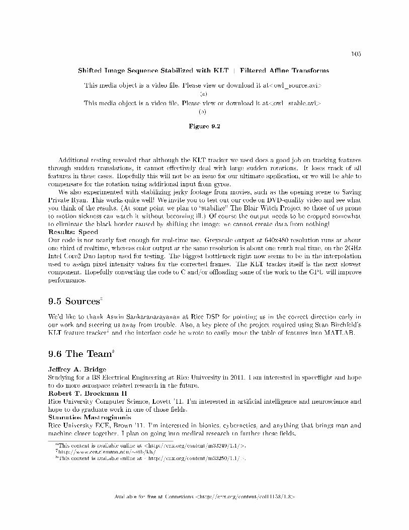
105
Shifted Image Sequence Stabilized with KLT + Filtered A�ne Transforms
This media object is a video �le. Please view or download it at<owl_source.avi>(a)
This media object is a video �le. Please view or download it at<owl_stable.avi>(b)
Figure 9.2
Additional testing revealed that although the KLT tracker we used does a good job on tracking featuresthrough sudden translations, it cannot e�ectively deal with large sudden rotations. It loses track of allfeatures in these cases. Hopefully this will not be an issue for our ultimate application, or we will be able tocompensate for the rotation using additional input from gyros.
We also experimented with stabilizing jerky footage from movies, such as the opening scene to SavingPrivate Ryan. This works quite well! We invite you to test out our code on DVD-quality video and see whatyou think of the results. (At some point we plan to �stabilize� The Blair Witch Project so those of us proneto motion sickness can watch it without becoming ill.) Of course the output needs to be cropped somewhatto eliminate the black border caused by shifting the image: we cannot create data from nothing!Results: SpeedOur code is not nearly fast enough for real-time use. Greyscale output at 640x480 resolution runs at aboutone-third of realtime, whereas color output at the same resolution is about one-tenth real time, on the 2GHzIntel Core2 Duo laptop used for testing. The biggest bottleneck right now seems to be in the interpolationused to assign pixel intensity values for the corrected frames. The KLT tracker itself is the next slowestcomponent. Hopefully converting the code to C and/or o�oading some of the work to the GPU will improveperformance.
9.5 Sources6
We'd like to thank Aswin Sankaranarayanan at Rice DSP for pointing us in the correct direction early inour work and steering us away from trouble. Also, a key piece of the project required using Stan Birchfeld'sKLT feature tracker7 and the interface code he wrote to easily move the table of features into MATLAB.
9.6 The Team8
Je�rey A. BridgeStudying for a BS Electrical Engineering at Rice University in 2011. I am interested in space�ight and hopeto do more aerospace related research in the future.Robert T. Brockman IIRice University Computer Science, Lovett '11. I'm interested in arti�cial intelligence and neuroscience andhope to do graduate work in one of those �elds.Stamatios MastrogiannisRice University ECE, Brown '11. I'm interested in bionics, cybernetics, and anything that brings man andmachine closer together. I plan on going into medical research to further these �elds.
6This content is available online at <http://cnx.org/content/m33249/1.1/>.7http://www.ces.clemson.edu/∼stb/klt/8This content is available online at <http://cnx.org/content/m33250/1.1/>.
Available for free at Connexions <http://cnx.org/content/col11153/1.3>

106 CHAPTER 9. VIDEO STABILIZATION
9.7 Code9
The main pieces of code used to accomplish the stabilization are shown below. There are several addition�les needed for the complete program, which are available for download instead of being shown inline:
• tracker.c10
• im2_jpeg.c11
• imload_bw.m12
• write_jpeg_bw.m13
• write_jpeg_col.m14
l2a�.m
% Least Squares Affine Transformation
% ELEC 301 Group Project
% 11/29/2009
% Jeffrey Bridge, Robert Brockman II, Stamatios Mastrogiannis
%
% Calculate the least squares affine transformation for two corresponding
% sets of pixel locations.
% px inputs are of the form:
%[ x_1 y_1
% x_2 y_2
% : :
% x_N y_N ]
%
% [x'] = [a, b] * [x] + [e]
% [y'] [c, d] [y] [f]
function Aff = l2aff(pxold, pxnew)
b = reshape(pxnew.', [], 1);
A = makenice(pxold);
x = pinv(A) * b; % Was psinv, our version of computing the pseudoinv
Aff = [x(1), x(2), x(5); ...
x(3), x(4), x(6)];
return
function A = makenice(pxold)
[r, c] = size(pxold);
A = zeros(2*r, 6);
for k=1:r
x = pxold(k,1);
y = pxold(k,2);
%correspond to a, b, c, d, e, f
A(2*k-1, :) = [x, y, 0, 0, 1, 0];
A(2*k , :) = [0, 0, x, y, 0, 1];
end
return
9This content is available online at <http://cnx.org/content/m33253/1.1/>.10See the �le at <http://cnx.org/content/m33253/latest/tracker.c>11See the �le at <http://cnx.org/content/m33253/latest/im2_jpeg.c>12See the �le at <http://cnx.org/content/m33253/latest/imload_bw.m>13See the �le at <http://cnx.org/content/m33253/latest/write_jpeg_bw.m>14See the �le at <http://cnx.org/content/m33253/latest/write_jpeg_col.m>
Available for free at Connexions <http://cnx.org/content/col11153/1.3>

107
a�_mul.m
% ELEC 301 Group Project
% 2009 December 12
% Jeffrey Bridge, Robert Brockman II, Stamatios Mastrogiannis
%
% Combine two affine transforms into one
%
% Aff = [a b e
% c d f]
%
% [x'] = [a, b] * [x] + [e]
% [y'] [c, d] [y] [f]
function Aff = aff_mul(Aff2, Aff1)
a1 = Aff1(1,1);
b1 = Aff1(1,2);
c1 = Aff1(2,1);
d1 = Aff1(2,2);
e1 = Aff1(1,3);
f1 = Aff1(2,3);
a2 = Aff2(1,1);
b2 = Aff2(1,2);
c2 = Aff2(2,1);
d2 = Aff2(2,2);
e2 = Aff2(1,3);
f2 = Aff2(2,3);
Aff = [...
a2*a1 + b2*c1, ...
a2*b1 + b2*d1, ...
a2*e1 + e2; ...
c2*d1 + c2*a1, ...
c2*b1 + d1*d2, ...
d2*f1 + f2];
return
stabilize.m
% Perform video stabilization on a set of jpeg images
% ELEC 301 Group Project
% 11/29/2009
% Jeffrey Bridge, Robert Brockman II, Stamatios Mastrogiannis
%
% Uses KLT features generated via track_destabilize.sh
% or track_movie.sh
% Reads destabilized stream of jpegs from stabilize_input
% Outputs stabilized stream of jpegs to stabilize_output
%
% Use view_stabilize.sh to play back results
%
function stabilize()
Available for free at Connexions <http://cnx.org/content/col11153/1.3>

108 CHAPTER 9. VIDEO STABILIZATION
% Read feature table. x and y contain coordinates of each feature
% for each frame. val is used to determine whether a feature has been
% replaced.
[x,y,val] = klt_read_featuretable('stabilize_input/features.txt');
% x, y are sets of column vectors, which we like.
% Extract number of features and frames from feature table.
[nFeatures, nFrames] = size(x);
invalid_inds = [];
% Each frame will have an affine transformation which allows it
% to be transformed back into the coordinates of the original frame.
% (These transforms will then be filtered to keep low-speed drift.)
Affs = zeros(nFrames,6);
% Affine transformation starts out as the identity transformation.
myAff = [1 0 0; 0 1 0];
% Iterate over all input frames
for n = 2:nFrames
fprintf('processing features for frame %d...', n);
% Position of features in previous frame.
pxold = [ x(:,n-1) y(:,n-1) ];
% Position of features in new frame.
pxnew = [ x(:,n) y(:,n)];
% Features which have replaced those that have left the scene
% have non-zero values in the feature table. These must be excluded
% from computing our affine transformation
ind = find(val(:,n) ∼= 0);
invalid_inds = ind;
% These are the indices of valid rows in our feature table
valid_inds = setdiff([1:nFeatures].', invalid_inds);
fprintf(' only %d features left\n', length(valid_inds));
% Extract valid features.
valid_pxold = pxold(valid_inds,:);
valid_pxnew = pxnew(valid_inds,:);
% Compute affine transformation which minimizes least squares
% difference in distances between features in the previous frame
% vs. the new frame transformed back to the original coordinates.
aff = l2aff(valid_pxold, valid_pxnew);
% Combine this "frame-by-frame" transformation with those from
% all previous frames to get an affine transformation that will
% transform the current frame into the coordinate system of the
Available for free at Connexions <http://cnx.org/content/col11153/1.3>

109
% FIRST frame.
myAff = aff_mul(aff, myAff);
% Make the resulting transform into a vector for ease of filtering
% and add it to the array of transforms for each frame.
Affs(n,:) = reshape(myAff,1,[]);
end
% High-pass filter the series of affine transformations to allow low
% frequency movement (panning, etc.) to show up in the final output.
%
% We do this by first low-pass filtering the series and then subtracting
% the result from the original.
%%{
switch 2 % Choose a filter
case 1 % Butterworth filter
[b, a] = butter(4,.05);
case 2 % Gaussian filter
b = exp(-linspace(-3,3,41).^2/2);
b = b / sum(b);
a = [1];
otherwise
error('Bad filter number');
end
filter_a = a;
filter_b = b;
% Pad beginning of transformation series with identity transforms
% to eliminate startup distortion.
eyeAff = [1 0 0 1 0 0];
prepCount = 1;
filtinAffs = [eyeAff(ones(prepCount,1),:); Affs(2:end,:)];
% LFP the affine transforms TWICE, the second time in time-reversed
% sequence. This eliminates phase distortion caused by the filter.
LpAffs = filtfilt(filter_b, filter_a, filtinAffs);
LpAffs = LpAffs(prepCount:end,:); % Remove padding
% HPF by subtracting LPF'd series from original.
Affs = Affs - LpAffs;
% Add back 1's in corners of rotation matrix component of transform
% removed by LPF. (Add back in identity transform)
Affs(:,1) = Affs(:,1) + 1;
Affs(:,4) = Affs(:,4) + 1;
%}
% Apply affine transforms to each frame to provide video stabilization.
%%{
for n = 2:nFrames
Available for free at Connexions <http://cnx.org/content/col11153/1.3>
110 CHAPTER 9. VIDEO STABILIZATION
% Get transform back into matrix form.
aff = reshape(Affs(n,:),2,3);
fprintf('interpolating image %d...\n', n);
disp(aff);
filename = sprintf('stabilize_input/D%08d.jpg', n);
% Black and white output is 3x faster to compute.
if 1
A = imread(filename);
Ar = single(A(:,:,1));
Ag = single(A(:,:,2));
Ab = single(A(:,:,3));
%B is image in coordinate system of first frame.
Br = im_unaff(Ar, aff);
Bg = im_unaff(Ag, aff);
Bb = im_unaff(Ab, aff);
B = cat(3,Br,Bg,Bb);
write_jpeg_col(B,sprintf('stabilize_output/S%08d.jpg',n));
else
A = imload_bw(filename);
B = im_unaff(A, aff);
write_jpeg_bw(B,sprintf('stabilize_output/S%08d.jpg',n));
end
end
%}
return
destabilize.m
% Generate Synthetic unstable test data
% ELEC 301 Group Project
% 11/29/2009
% Jeffrey Bridge, Robert Brockman II, Stamatios Mastrogiannis
function destabilize()
% Load a big source image, and split it into colors
filename = 'destabilize_input.jpg';
A = imread(filename);
Ar = single(A(:,:,1));
Ag = single(A(:,:,2));
Ab = single(A(:,:,3));
% Size of output image to generate, a subset of the source image
output_w = 560;
output_h = 400;
% Center of source image
[r,c] = size(Ar);
Available for free at Connexions <http://cnx.org/content/col11153/1.3>

111
center_row = r/2;% - 50;
center_col = c/2;
% Number of output frames to generate
N = 300;
% Standard deviation of jerky movement in pixels
dev = 5;
% Parameters controlling slow drift
drift_radius = 10;
drift_period = 100;
for n = 1:N
fprintf('Generating destabilized image %d...\n', n);
% Add in slow drift of the image center
drift_rows = drift_radius * sin(n*2*pi/drift_period);
drift_cols = drift_radius * cos(n*2*pi/drift_period);
% Add in fast random jerky movements
offset_rows = floor(randn(1) * dev);
offset_cols = floor(randn(1) * dev);
% Calculate current image boundaries
left = floor(center_col + drift_cols - output_w/2 + offset_cols);
right = left + output_w - 1;
top = floor(center_row + drift_rows - output_h/2 + offset_rows);
bottom = top + output_h - 1;
% Grab an offset portion of the larger image
Br = Ar(top:bottom, left:right);
Bg = Ag(top:bottom, left:right);
Bb = Ab(top:bottom, left:right);
% Save it to its own file
B = cat(3,Br,Bg,Bb);
write_jpeg_col(B,sprintf('destabilize_output/D%08d.jpg',n));
% Play back with view_destabilize.sh
end
return
im_una�.m
% IMage UNdo an AFFine transformation
% ELEC 301 Group Project
% 11/29/2009
% Jeffrey Bridge, Robert Brockman II, Stamatios Mastrogiannis
%
% --- INPUTS ---
% Z = image matrix (2D grid of intensities)
% Aff = affine transformation
Available for free at Connexions <http://cnx.org/content/col11153/1.3>

112 CHAPTER 9. VIDEO STABILIZATION
% [a b e
% c d f]
% [x'] = [a b]*[x] + [e]
% [y'] [c d] [y] [f]
%
% --- OUTPUTS ---
% ZI = output image matrix
function ZI = im_unaff(Z, Aff)
% Extract size of image.
[r,c] = size(Z);
% Extract affine transformation coefficients.
Aa = Aff(1,1);
Ab = Aff(1,2);
Ac = Aff(2,1);
Ad = Aff(2,2);
Ae = Aff(1,3);
Af = Aff(2,3);
% generate new sets of grid points
[X0,Y0] = meshgrid(1:c, 1:r);
% XI(c,r) and YI(c,r) contain where to look in Z for the correct
% intensity value to place in the new image ZI at coordinates (r,c).
XI = Aa*X0 + Ab*Y0 + Ae;
YI = Ac*X0 + Ad*Y0 + Af;
% Since XI and YI contain non-integer values, a simple lookup will not
% suffice. We must perform interpolation.
ZI = interp2(Z, XI, YI);
return
9.8 Future Work15
Future WorkNow that we basic algorithms down, the focus should be on improving the speed so we can get real-timestabilized video feed while operating our UAV. This means converting the code to C. It may also be necessaryto use KLT trackers that use the video card GPU, as well as writing an equivalent of the MATLAB interp2that does the same.
While taking the �rst steps towards this conversion, we realized that our video stabilizer would makea pretty cool GStreamer plugin. GStreamer16 is a media framework for the open-sourse Gnome desktopenvironment. With it, we will be able route video sources of many kinds through our stabilizer and then onto our choice of video sinks. We have already �gured out how to implement a "null" plugin that just copiesframes from the source to the sink already, so once our algorithms are in C using GStreamer should be easy.
If these improvements can be made, the next step will be to test the code out with live footage from ourown UAV.
15This content is available online at <http://cnx.org/content/m33254/1.1/>.16http://gstreamer.freedesktop.org/
Available for free at Connexions <http://cnx.org/content/col11153/1.3>

Chapter 10
Facial Recognition using Eigenfaces
10.1 Facial Recognition using Eigenfaces: Introduction1
10.1.1 Introduction
10.1.1.1 Facial Recognition Preface
Although humans have an amazing ability to distinguish and recognize faces, facial recognition on computersis an advanced �eld of study yet to be perfected. Only within the past decade have people seen the rise offace tracking in digital cameras and public security systems. Unlike humans, computers are easily confusedby changes in illumination, variation in face angles, and accessories such as hair, glasses, and hats. However,computer face recognition is worth pursuing, because of the wealth of applications in security, digital pho-tography, social networking, and other �elds. This project uses the eigenface method to identify faces fromstill images.
1This content is available online at <http://cnx.org/content/m33173/1.3/>.
Available for free at Connexions <http://cnx.org/content/col11153/1.3>
113
114 CHAPTER 10. FACIAL RECOGNITION USING EIGENFACES
Figure 10.1: A potential face recognition/X-Ray technology application.
10.1.1.2 Facial Recognition Approach
When considering the proper approach for identifying faces, it was decided that the approach to be able todeal with imperfect settings such as di�erent relative positions, sizes, and shapes of facial features such asthe eyes, nose, cheekbones, and jaw. While facial features are a major component of some facial recognitionalgorithms, the extraction of landmarks were determined to be insu�ciently robust for this project withouta powerful normalization algorithm capable of features such as keeping a constant light intensity, correctionof angles and pose variations, and accounting for accessories like glasses.
10.2 Facial Recognition using Eigenfaces: Background2
10.2.1 Background
10.2.1.1 Computational Implementations
Current facial recognition algorithms can be separated into two groups: geometric and statistical. Thegeometric approach looks into the distinguishing features of the face. The other algorithms are photometric,a statistical approach that distills an image into values and compares those values with those from a templateor training set to eliminate variances. Some popular recognition algorithms include Principal ComponentAnalysis (eigenfaces), Linear Discriminate Analysis, Elastic Bunch Graph Matching (�sherfaces), the HiddenMarkov model, and dynamic link matching.
10.2.1.2 Eigenfaces
We decided to use eigenfaces for this project. Eigenfaces are created using a statistical tool called PrincipalComponent Analysis (PCA). Eigenfaces are useful because they focus on the di�erences between the
2This content is available online at <http://cnx.org/content/m33174/1.5/>.
Available for free at Connexions <http://cnx.org/content/col11153/1.3>

115
data points (i.e., the small variations in eye shape, nose size, and skin color that humans unconsciously ande�ectively use to tell each other apart). Eigenfaces can be speedily extracted from large data sets, so thismethod is very applicable to our project.
However, the eigenface method has one major drawback: it is greatly a�ected by non-homogenous condi-tions. For example, Matthew Turk and Alex Pentland of MIT found that the eigenface approach identi�eda face correctly 96% of the time with lighting variation, 85% with orientation variation, and only 64% withsize variation (1). Therefore, we decided to focus on one variable: lighting, background, face angle, position,or expression, and keep all the others constant. Our pictures were taken in a well-lit room against a whitebackground, with the subject directly facing the camera, without accessories such as hats and glasses. Wefound that facial expressions were the most fun variable and decided to focus on that.
We worked with two databases: Rice University, which we created, and JAFFE (Japanese Female Fa-cial Expression) from http://face-rec.org/3 . The JAFFE database consists of 10 Japanese women, eachexpressing each of seven emotions. For the Rice database, we chose students of both genders and diverseethnicities. Each subject was told to express each of six emotions: neutral, happy, sad, surprised, angry, anddisgusted. We had sixteen subjects, each with six emotions, and we took two pictures per emotion, resultingin a database of 192 images. We used Matlab to process the images and create eigenfaces.
10.3 Facial Recognition using Eigenfaces: Obtaining Eigenfaces4
10.3.1 Obtaining Eigenfaces
10.3.1.1 Eigenface Concept
Each image is loaded into a computer as a matrix of di�erent intensities. All the images were converted togray scale so that we only need to operate on one layer of image (instead of three layers for a RBG image).A vector whose direction is unchanged when multiplied by the matrix is referred to as an eigenvector of thatmatrix. The eigenvectors of the covariance matrix associated with a large set of faces are called eigenfaces.The eigenfaces can be thought of as a basis for the set of faces. Just as any vector in a vector space iscomposed of a linear combination of the basis vectors, each face in the set can be expressed as a linearcombination of the eigenfaces.
10.3.1.2 Format Input Data
To compute the eigenfaces, a portion of a given dataset is �rst chosen randomly to be the training set. Theimages in the training set are used to construct the image matrix A (Note: All images in the dataset musthave the same dimensions). The training set can be chosen by selecting a given percentage of the datasetor by selecting a given number of images per person from the database. Once the images are selected, eachimage I i is vectorized into a column vector Pi such that its length equals to the total number of pixels in theimage. This process brings the mathematics of all the computations down to a lower-dimensionality space.
I = N ×M ⇒ Pi = 1×NM (10.1)
3http://face-rec.org/4This content is available online at <http://cnx.org/content/m33183/1.6/>.
Available for free at Connexions <http://cnx.org/content/col11153/1.3>

116 CHAPTER 10. FACIAL RECOGNITION USING EIGENFACES
Figure 10.2: Sample training images
The mean face of the training set is computed and subtracted from all the images within the training set(given W images in the training set).
µ =1W
W∑i=0
Pi (10.2)
Vi = Pi − µ (10.3)
Figure 10.3: Mean face of HFH dataset
Finally, the mean subtracted training images are put into a single matrix of dimension NM x W, formingthe image matrix A.
A =[V1 V2 V3 ... VW
](10.4)
10.3.1.3 Compute Eigenfaces
Typical PCA calculation would �rst retrieve the covariance matrix C. Covariance measures the relation ofhow much two random variables vary together such that if the covariance is positive when both dimensions
Available for free at Connexions <http://cnx.org/content/col11153/1.3>

117
increase together and negative when they are inversely proportional. The eigenfaces were then obtained bycomputing the eigenvectors of the covariance matrix C. This computation will yield NM unique eigenvectors.
C = AAT (10.5)
cov (X,Y ) =∑
(xi − x) (yi − y)n− 1
(10.6)
But in the case of this project, these resulting matrix of dimension NM x NM was way too large forMATLAB to process. Furthermore, even if MATLAB had the ability to process such a large matrix it wouldstill later be too computationally intensive. Instead of computing the covariance matrix C directly, thisproject utilizes a smaller matrix S with dimensions W x W that can still be able to compute the eigenfacese�ciently. This simpli�cation stems from the fact that the rank of the covariance matrix C is limited by thenumber of images in the training set. Since there are at most W-1 non-trivial eigenfaces for C, there is noneed to compute all of the eigenfaces for the dataset. This simpli�cation will prove to be useful as long asNM�W.
S = ATA (10.7)
The smaller matrix dimensions will be computationally e�ective later when large databases will be sortedthrough since only W eigenvalues and eigenfaces will be used.
Now, using some linear algebra tricks, we could show that the eigenvalues of C and S are the same andthat the top W eigenvectors of C (ui) can be obtained from the eigenvectors of S (vi).
Svi = λivi
ATAvi = λivi
AATAvi = λiAvi
CAvi = λiAvi
Cui = λiui
(10.8)
In this manner, we can see that the eigenvectors of C can be derived from
Avi = ui (10.9)
where the computation of vi's were much less computationally extensive than the direct computation ofui's.
These ui vectors will constitute the columns of the eigenfaces.
Eigenface = [u1 u2 u3 ... uW
10.3.1.4 Top K Eigenfaces
Even with this complexity reduction, it is still redundant to use all W eigenfaces for the reconstructionprocess. We could reduce the number of eigenfaces used even more by indentifying the eigenfaces thatcontain more content than the others. To determine this property, we bring our attentions to the eigenvaluesthat correspond to the individual eigenfaces. We immediately see that there are some eigenfaces that havehigher eigenvalues than the others.
Available for free at Connexions <http://cnx.org/content/col11153/1.3>

118 CHAPTER 10. FACIAL RECOGNITION USING EIGENFACES
Figure 10.4: Eigenvalues of the corresponding eigenfaces of HFH dataset
After arranging the eigenvalues in descending order, the result becomes clearer. We conclude that theeigenfaces corresponding to high eigenvalues contain more content. In other words, the higher the eigenvalue,the more characteristic features of the face the particular eigenvector describes. Therefore, we simplify thereconstruction process by only using the top K eigenfaces. This completes the training process of ourimplementation.
Figure 10.5: Top 5 eigenfaces of HFH dataset
Available for free at Connexions <http://cnx.org/content/col11153/1.3>

119
Figure 10.6: Last 5 eigenfaces of HFH dataset
In terms of the eigenfaces themselves, we found that the more important eigenfaces (those with highereigenvalues) had lower spatial frequency than the less important eigenfaces (those with lower eigenvalues).This is apparent in the �gure above, where the �rst eigenfaces look blurry and indistinct, and the latereigenfaces have sharp edges and look more like individual people. This suggests that faces can be identi�edbased on their low-frequency components alone.
10.3.2 Eigenface Recognition Face Datasets
10.3.2.1 Test 1 (JAFFE database)
For the �rst test of this project's eigenface generation algorithm, the Japanese Female Facial Expression(JAFFE) Database was used. The JAFFE database �t our ideal conditions of similar lighting conditions,solid white backgrounds, and normalization of facial features such as the nose, eyes, and lips. The databaseis a set of 180 images of seven facial expressions (six basic facial expressions and one neutral).
10.3.2.2 Test 2 (Rice University)
For the Rice database, we chose students of both genders and diverse ethnicities. Each subject was told toexpress each of six emotions: neutral, happy, sad, surprised, angry, and disgusted. We had sixteen subjects,each with six emotions, and we took two pictures per emotion, resulting in a database of 192 images. We alsocreated a special database of two emotions: closed eyes and expression of choice, to be used for demonstrationat the poster session.
Available for free at Connexions <http://cnx.org/content/col11153/1.3>

120 CHAPTER 10. FACIAL RECOGNITION USING EIGENFACES
10.3.2.3 Algorithm Concept
Figure 10.7: Diagram of eigenface computation and input with our algorithm. Also, a visual represen-tation of K-dimensional �face space� and threshold setting between test image reconstruction (red dot)and closest match image reconstruction (blue dot)
10.4 Facial Recognition using Eigenfaces: Projection onto FaceSpace5
10.4.1 Projection onto Face Space
10.4.1.1 Compute Weight Matrix
Now that we have the eigenfaces, we could proceed to projecting the training images onto the face space.The K-dimension face space is spanned with the top K eigenfaces. An interesting thing to note here is thateach axis of the face space is weighted with respect to the eigenvalue associated with it. So the �rst few axeswill contain more weight than the later axes.
To project the mean-subtracted training images Vi's onto the face space, we �rst take each image andcompute its weight wi on each of the axis by taking the dot product between the image and an eigenface.This process is repeated for each eigenface with each training image. The resulting weights are put into aweight matrix WM with a dimension of K x W.
Vj = w1u1 + w2u2 + ...+ wkuk (10.10)
5This content is available online at <http://cnx.org/content/m33182/1.6/>.
Available for free at Connexions <http://cnx.org/content/col11153/1.3>

121
WM =
(w1)V1(w1)V2
... (w1)VW
(w2)V1(w2)V2
... (w2)VW
(w3)V1(w3)V2
... (w3)VW
... ... ... ...
(wk)V1(wk)V2
... (wk)VW
(10.11)
Figure 10.8: Projection of training images (blue dots) and test image (red dot) onto the 3-dimensionalface space
10.4.1.2 Compute Threshold Values
When given a test image (red dot), it is �rst projected onto the face space using the same method as beforeand then categorized using some threshold values. By testing these and graphing the minimum distancebetween each test image and the closest image in the training set, we were able to experimentally come upwith the thresholds. The following graph shows the result of a particular run on the HFH dataset.
Available for free at Connexions <http://cnx.org/content/col11153/1.3>
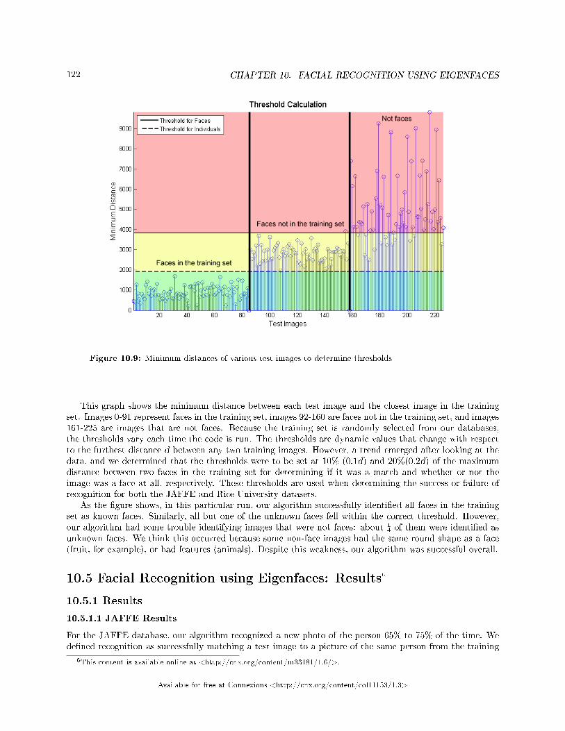
122 CHAPTER 10. FACIAL RECOGNITION USING EIGENFACES
Figure 10.9: Minimum distances of various test images to determine thresholds
This graph shows the minimum distance between each test image and the closest image in the trainingset. Images 0-91 represent faces in the training set, images 92-160 are faces not in the training set, and images161-225 are images that are not faces. Because the training set is randomly selected from our databases,the thresholds vary each time the code is run. The thresholds are dynamic values that change with respectto the furthest distance d between any two training images. However, a trend emerged after looking at thedata, and we determined that the thresholds were to be set at 10% (0.1d) and 20%(0.2d) of the maximumdistance between two faces in the training set for determining if it was a match and whether or not theimage was a face at all, respectively. These thresholds are used when determining the success or failure ofrecognition for both the JAFFE and Rice University datasets.
As the �gure shows, in this particular run, our algorithm successfully identi�ed all faces in the trainingset as known faces. Similarly, all but one of the unknown faces fell within the correct threshold. However,our algorithm had some trouble identifying images that were not faces: about ¼ of them were identi�ed asunknown faces. We think this occurred because some non-face images had the same round shape as a face(fruit, for example), or had features (animals). Despite this weakness, our algorithm was successful overall.
10.5 Facial Recognition using Eigenfaces: Results6
10.5.1 Results
10.5.1.1 JAFFE Results
For the JAFFE database, our algorithm recognized a new photo of the person 65% to 75% of the time. Wede�ned recognition as successfully matching a test image to a picture of the same person from the training
6This content is available online at <http://cnx.org/content/m33181/1.6/>.
Available for free at Connexions <http://cnx.org/content/col11153/1.3>

123
set, even though the two images had di�erent expressions. Recognition rate increased dramatically as weincreased the number of eigenfaces, but stabilized after four eigenfaces (that is, our recognition rate didnot increase by using more than four eigenfaces). The recognition rate also increased when we used moretest images per person in the training set. Similarly, the recognition rate increased when we used a greaterpercentage of the dataset in the training set (with pictures chosen randomly from the dataset).
Figure 10.10: Results when varying the number of training images per person & the percent of databaseused to as input images
10.5.1.2 Rice University Field Test Results
For the Rice University database, our algorithm recognized a new photo of the person 65% to 75% of thetime. Again, recognition rate increased dramatically as we increased the number of eigenfaces. In this case,the recognition rate stabilized after six eigenfaces. The recognition rate required more eigenfaces to stabilizebecause the Rice database was more diverse, including people of both genders and many di�erent ethnicities.Therefore, more eigenfaces are needed for an accurate representation of the Rice population. Again, therecognition rate increased when we used more test images per person in the training set. The recognitionrate also increased when we used a greater percentage of the dataset in the training set.
Available for free at Connexions <http://cnx.org/content/col11153/1.3>

124 CHAPTER 10. FACIAL RECOGNITION USING EIGENFACES
Figure 10.11: Results when varying the number of training images per person & the percent of databaseused to as input images
The resulting �nal algorithm was able to determine, at the four rates shown in the previous two �gures,whether a test image was a non-face or face and also a match to known face, �nding the closest match to aknown face (as shown below).
Available for free at Connexions <http://cnx.org/content/col11153/1.3>
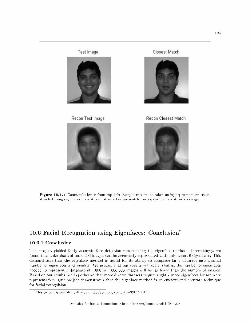
125
Figure 10.12: Counterclockwise from top left: Sample test image taken as input; test image recon-structed using eigenfaces; closest reconstructed image match; corresponding closest match image.
10.6 Facial Recognition using Eigenfaces: Conclusion7
10.6.1 Conclusion
This project yielded fairly accurate face detection results using the eigenface method. Interestingly, wefound that a database of some 200 images can be accurately represented with only about 6 eigenfaces. Thisdemonstrates that the eigenface method is useful for its ability to compress large datasets into a smallnumber of eigenfaces and weights. We predict that our results will scale, that is, the number of eigenfacesneeded to represent a database of 1,000 or 1,000,000 images will be far fewer than the number of images.Based on our results, we hypothesize that more diverse datasets require slightly more eigenfaces for accuraterepresentation. Our project demonstrates that the eigenface method is an e�cient and accurate techniquefor facial recognition.
7This content is available online at <http://cnx.org/content/m33177/1.4/>.
Available for free at Connexions <http://cnx.org/content/col11153/1.3>

126 CHAPTER 10. FACIAL RECOGNITION USING EIGENFACES
10.6.1.1 Further work
To improve the results of the eigenface method implemented, a normalization program could be developed todetermine the facial metrics and normalize the photos such that facial features are held in constant positionsand contrast and light intensities between photos are balanced. Localizing of the features would keep headpositions fairly consistent and yield better eigenfaces.
Creating a program to extract faces from their environment (for example, by using a matched �lter)would expand the possible applications of this project. Individual faces could be extracted from securitycameras or group pictures.
A larger and more diverse dataset would also increase face identi�cation and recognition. We would liketo include people of diverse ages, since everyone in both the JAFFE and Rice datasets was in their teens ortwenties. Increasing the size and quality of the dataset would boost the recognition rate. We would like tosee how many eigenfaces are needed to represent a dataset of 1,000 or 1,000,000 images.
Because both our datasets have emotions as a variable, it would be interesting to create an �emotiondetector�, as was done with the JAFFE data. Despite the fact that emotions look di�erent on every person(fear was found to be an especially problematic emotion), emotion recognition rates of over 67% wereattainedusing Gabor wavelets2 . It would be interesting to see how the eigenface method compares.
10.6.2 Facial Recognition Source Codes
• If you would like to try out out our facial recognition code for yourself, you can download them here8.This code allows you to input one test image and matches it to the closest image in the given dataset.The JAFFE dataset is included for testing.
• If you would like to test with our full code or to obtain the HFH dataset, please contact Aron Yu([email protected] )
• GUI version of the code coming soon...
10.7 Facial Recognition using Eigenfaces: References andAcknowledgements10
10.7.1 References and Acknowledgements
Team members:
• Catherine Elder ([email protected])• Norman Pai ([email protected])• Je�rey Yeh ([email protected])• Yingbo �Aron� Yu ([email protected])
We would like to thank Manjari Narayan, our advisor for this project, for all her help. Finally, we would liketo thank professor Richard Baraniuk and Matthew Moravec for the opportunity to work on this project.
10.7.1.1 References
1. Zhao, W. et al. "Face Recognition: A Literature Survey." ACM Computing Surveys, Vol. 35, No. 4,December 2003, pp. 399�458
2. M. Turk and A. Pentland (1991). "Face recognition using eigenfaces11 ". Proc. IEEE Conference onComputer Vision and Pattern Recognition. pp. 586�591
8See the �le at <http://cnx.org/content/m33177/latest/SingleRun.rar>[email protected]
10This content is available online at <http://cnx.org/content/m33180/1.3/>.11http://www.cs.ucsb.edu/∼mturk/Papers/mturk-CVPR91.pdf
Available for free at Connexions <http://cnx.org/content/col11153/1.3>

127
3. JAFFE image database � "Coding Facial Expressions with Gabor Wavelets�, Michael J. Lyons, ShigeruAkamatsu, Miyuki Kamachi, Jiro Gyoba < http://www.kasrl.org/ja�e.html12 >.
4. �Introduction to Fourier Transforms for Image Processing.� <http://www.cs.unm.edu/∼brayer/vision/fourier.html13>.
5. �Face Recognition Using Eigenfaces.� <http://www.cs.princeton.edu/∼cdecoro/eigenfaces/14 >.6. Pissarenko, Dimitri. �Eigenface-based facial recognition.� <http://openbio.sourceforge.net/resources/eigenfaces/eigenfaces-
html/facesOptions.html15 >.
12http://www.kasrl.org/ja�e.html13http://www.cs.unm.edu/∼brayer/vision/fourier.html14http://www.cs.princeton.edu/∼cdecoro/eigenfaces/15http://openbio.sourceforge.net/resources/eigenfaces/eigenfaces-html/facesOptions.html
Available for free at Connexions <http://cnx.org/content/col11153/1.3>

128 CHAPTER 10. FACIAL RECOGNITION USING EIGENFACES
Available for free at Connexions <http://cnx.org/content/col11153/1.3>

Chapter 11
Speak and Sing
11.1 Speak and Sing - Introduction1
11.1.1 Speech Scaling and Pitch Correction
The speech scaling and pitch correction program, or �Speak & Sing�, generates a properly-timed and pitch-accurate sample of a known song from recorded spoken words.
A voice modulation application which detects the timing and pitch of the recorded input and automat-ically performs time scaling and pitch correction to match the speech to a pre-selected song, producing amusical output.
11.1.1.1 Making a Smarter Autotuner
Pitch correction is used by musicians to improve the sound of song vocals by �xing o�-key singing or addingdistortion. It can be applied real-time using a synthesizer keyboard or added after recording. However, these�autotuners� can't �x o�-tempo singing, and automatic autotuners depend on the singer to be relativelyclose to the right pitch.
Goals for the Speak and Sing:
• Proof-of-concept of automated syllable detection, time scaling, and pitch correction in one robustapplication
• Provides open-ended, customizable options for audio processing• Demonstrates time and frequency DSP applications using MatLab
11.1.1.2 Implementation: An Overview
Recording:Input voice samples are recorded in mono-channel audio at a sampling frequency of 16,000 (although any
sampling frequency can be used). It is then imported into MatLab and the following functions are run insequence:
Song Interpretation and Retrieval:Contains data for selected songs based on sheet music. It returns a vector of fundamental note frequencies
and note lengths depending on the song selected and the desired tempo.Available Songs:1. Christina Aguilera - Genie in a Bottle2. Mary Had a Little Lamb
1This content is available online at <http://cnx.org/content/m33229/1.1/>.
Available for free at Connexions <http://cnx.org/content/col11153/1.3>
129

130 CHAPTER 11. SPEAK AND SING
3. Row, Row, Row Your BoatSyllable DetectionAnalyzes the input speech data and determines the locations and lengths of each syllable. After dividing
the signal up into several short windowed pieces, it detects the periodicity and energy of each window todetermine the type of sound (vowel, consonant, or noise). The locations of the syllables is then determinedbased on the pattern of sounds.
Time scalingInterprets the detected syllable locations and stretches or shrinks the syllable to match the length of the
word in the song. The time scaling is performed using a time-domain Waveform Similarity Overlap Add(WSOLA) algorithm, which breaks up the signal into overlapping windows and copies each window to anew location, either closer together or further apart. This stretches or compresses the length of the speechwithout losing quality or information.
Pitch correctionDetects the pitch of the signal, compares it to the desired pitch of the song, and makes pitch corrections.
Pitch detection is done using FAST-autocorrelation, in which small windows of the signal are o�set andautocorrelated to �nd the period, and thus frequency, of the signal for that interval. Pitch correctionis performed with Pitch Synchronous Overlap Add (PSOLA), which moves windowed segments closer orfurther apart and overlap-added to alter the frequency without loss of sound.
11.1.1.3 The Result
The resulting audio �le sounds like the input speech or singing, but the words will now line up with those ofthe original song and the pitch will be adjusted. The resulting impact on sound is that the recorded inputwill now sound more like the song, without compromising the original voice or speech.
11.2 Speak and Sing - Recording Procedure2
11.2.1 Recording
Input voice samples are recorded in mono-channel audio with a sampling frequency of 16,000 Hz. Thesampling rate chosen allows for a balance of processing e�ciency and sound quality � the computation timeof the program generally scales linearly with increase in sampling rate. The selected sampling frequency isalso convenient for computation, as the MatLab program's wave audio operations perform best with samplingfrequencies in increments of 8,000 Hz. The program allows for the use of any sampling frequency and willperform adequately for sampling frequencies up to and beyond the audio standard 44.1 kHz, but processingtime and program durability become an issue.
When recording, the best results are produced for input speech or song which is delivered slowly andclearly, with either brief pauses or strongly-enunciated consonants between syllables and words.
The recorded sound is processed in Audacity, a freeware recording software, to trim out excess electricaland environmental noise and remove existing DC o�sets. It is then ready for handling in the MatLabenvironment.
11.3 Speak and Sing - Song Interpretation3
11.3.1 Song Interpretation
The songs to be used by the Speak and Sing were predetermined and preprogrammed. For simplicity, thesongs feature a one-to-one format. That means every syllable of the lyrics is associated with one durationand one pitch, there are no rests and no slurs. The song interpretation is done in two vectors, one contains
2This content is available online at <http://cnx.org/content/m33233/1.1/>.3This content is available online at <http://cnx.org/content/m33237/1.1/>.
Available for free at Connexions <http://cnx.org/content/col11153/1.3>

131
all of the durations (in seconds) to be used by the duration matching, and the other contains all of the notefrequencies (in hertz) to be used by the pitch matching.
Here is an example of a measure of sheet music that has been turned into a useable vector.
Mary Had a Little Lamb
Figure 11.1
notes = ([246.94; 220;196; 220; 246.94; 246.94; 246.94;]);
duration = ([.5; .5; .5; .5; .5; .5; .5;]);
Three songs were made available for use:1. Christina Aguilera - Genie in a Bottle2. Mary Had a Little Lamb3. Row, Row, Row Your Boat
11.4 Speak and Sing - Syllable Detection4
11.4.1 Syllable Detection
The syllable detection algorithm takes as its input recorded speech and produces an output matrix denotingthe start and end times of each syllable in the recording. There are two main parts to the algorithm. First,each sound in the input �le must be classi�ed as a vowel, consonant, or noise. Second, the algorithm mustdetermine which sequences of sounds correspond to valid syllables.
11.4.1.1 Sound Classi�cation
The sound classi�cation step splits the input signal into many small windows to be analyzed separately. Theclassi�cation of these windows as vowels, consonants, or noise relies on two core characteristics of the signal:energy and periodicity. Vowels stand out as having the highest energy and periodicity values, noise ideallyhas extremely low energy, and consonants are everything that falls between these two extremes.
The energy of a window of the input vector W is calculated as
E = |W|^2.
However it is necessary to set general energy thresholds that are valid for speech samples of varying volume.In order to accomplish this, after the energies of all the windows have been calculated, they are convertedinto decibels relative to the maximum energy value.
4This content is available online at <http://cnx.org/content/m33241/1.1/>.
Available for free at Connexions <http://cnx.org/content/col11153/1.3>

132 CHAPTER 11. SPEAK AND SING
E' = 10*log10(E/max(E)).
The energy thresholds are then de�ned in terms of a percent of the total energy range. For example, if anenergy threshold was 25 percent and the energies ranged from -100 to 0 dB, then everything from -25 to 0dB would be above the threshold.
In some cases, energy alone is enough to determine whether a certain sound is a vowel, consonant, ornoise. For instance, here is a plot of the energy vs. time of a recording of the spoken word "cat." It is easyto tell which portions of the �gure correspond to vowels, consonants, and noise by inspection:
Figure 11.2: The energy threshold clearly divides the high-energy vowel portion of the signal from theconsonants.
However, energy cannot always separate vowels and consonants so dramatically. For example, the word"zoo."
Available for free at Connexions <http://cnx.org/content/col11153/1.3>

133
Figure 11.3: The ending vowel sound drops too close to the threshold.
Although a portion of the vowel still has signi�cantly higher energy than the consonant, the endingportion of the vowel drops in energy to the point where it is dangerously close to the threshold. Raisingthe threshold so that the "z" sound is certain not to be counted as a vowel only makes it more likely thatportions of the "oo" sound will be mistakenly classi�ed as consonants. Clearly, additional steps are necessaryto more accurately di�erentiate between consonants and vowels.
11.4.1.2 Periodicity Analysis
The algorithm uses the periodicity of the signal to accomplish this task. The periodicity is obtained usingthe autocovariance of the window being analyzed. This is calculated as:
C(m) = E[(W(n+m)-mu)*conj(W(n)-mu)]
Mu is the mean of the window W. It measures how similar the signal is to itself at shifts of m samples and cantherefore distinguish periodic signals from aperiodic ones due to their repetitive nature. The autocovariancevector is most stable and therefore most meaningful for values of m relatively close to 0, since for larger m,fewer samples are considered, causing the results to become more random and unreliable. Therefore, the
Available for free at Connexions <http://cnx.org/content/col11153/1.3>

134 CHAPTER 11. SPEAK AND SING
sound classi�cation algorithm only considers autocovariance values with m less than 1/5 the total windowsize. These autocovariance values are normalized so that the value at m = 0 is 1, the largest possible value.The maximum autocovariance in this stable region is considered the periodicity of the window.
The periodicity values for vowels are extremely high, while most unvoiced, and some voiced, consonantsexhibit very low periodicity. Periodicity is especially useful in detecting fricative or a�ricate consonantswhich are both characterized by a great deal of random, possibly high-energy, noise due to their methodof articulation. Examples of these consonants include "s," "z," "j," and "ch." The contrast between theperiodicity of a fricative consonant and a vowel can be clearly seen in this plot.
Figure 11.4
Putting it all together, the sound classi�cation portion of the algorithm �rst calculates the energy andperiodicity of each window of the input signal. If both the energy and periodicity are higher than certainthresholds, the window is classi�ed as a vowel. If the energy is smaller than a very low threshold, the windowis counted as noise, and everything in between is considered a consonant. Let's take another look at theenergy characteristics of the word "zoo" (refer to �gure 2). Using this alone, we could not easily distinguishthe high-energy "z" from the lower-energy portion of the "oo." However, here is a plot of the periodicity vs.time for the same recording.
Available for free at Connexions <http://cnx.org/content/col11153/1.3>

135
Figure 11.5: The di�erence between the "z" and the "oo" is now much more pronounced.
This plot shows a clear contrast between the aperiodic fricative "z" and the periodic vowel. Takentogether, these data now provide su�cient information for the sound classi�cation algorithm to correctlyidentify each sound in this recording.
This method works with a reasonable degree of accuracy, but there are a few challenges that must beconsidered. The greatest among these is the handling of liquid consonants like "l," "y," or "m." In certaincases, these sounds are used as consonants at syllable boundaries, while in other circumstances, they act asa vowel usually would in making up the majority of the syllable. For example, in the word "little," the �rst"l" is acting as a consonant, but the "l" sound is also used as the central portion of the second syllable.Therefore, these sounds are not always accurately classi�ed, and they must be annunciated strongly in theinput recording if they are acting as syllable boundaries.
Another issue with this method is that sometimes it detects short bursts of one sound type in the middleof another. For instance, there may be 1 or 2 consonant windows surrounded by a large number of noisewindows or a small number of vowel windows in the middle of a large section of consonant windows. Severalsituations can lead to errors like this. For example, the background noise in a recording might boost theenergy of a window high enough to be classi�ed as a consonant, or random spikes in the periodicity of anotherwise aperiodic signal could cause part of a consonant to be classi�ed as a vowel. These errors can beminimized by imposing a length constraint on sounds. In order for a group of windows to be classi�ed asa particular sound, they must represent a long enough chunk of time to be considered meaningful. If thegroup of windows is too small, they are reclassi�ed to match the sound immediately preceding them.
Available for free at Connexions <http://cnx.org/content/col11153/1.3>

136 CHAPTER 11. SPEAK AND SING
11.4.1.3 Syllable Interpretation
After each sound in the input has been classi�ed, it is necessary to determine which sound sequences should beinterpreted as syllables. This is accomplished using a tree-like decision structure which examines consecutiveelements of the sound classi�cation vector, comparing them to all possible sequences. Once a known sequenceis identi�ed, it is added to the list of syllables, and the algorithm moves on to the next ungrouped sounds.The decision structure is depicted in the following �gure.
Figure 11.6
After this step, some syllables were occasionally much too short. For instance, the word "good" had asmall probability of being split up into two syllables ("goo"" and "d") depending on how much the speakeremphasizes the voicing of the d. Further increasing the minimum allowable sound duration caused too muchinformation to be lost or misinterpreted, so a minimum syllable duration parameter was also added. If asyllable is too short, it is combined with an adjacent syllable based on its surrounding sounds. If one ofthe sounds adjacent to the short syllable is noise and the other is not, the short syllable is added to theside without noise to preserve continuity of the signal. If neither sound adjacent to the syllable is noise,the duration of each adjacent sound is calculated, and the syllable is tacked onto the side with the shortestneighboring sound as this one is more likely to have been cut o� in error.
The following table lists the values for the various thresholds and parameters we found worked best forrelatively clean, noise-free, input signals. These parameters must be adjusted if a great deal of periodic orenergetic background noise, such as might be caused by a microphone picking up the sound of a computer
Available for free at Connexions <http://cnx.org/content/col11153/1.3>

137
fan, is expected to corrupt the input recording.
Parameter Value
Window length 5 ms
Vowel periodicity threshold .75
Vowel energy threshold 27% of total energy range
Noise energy threshold 55% of total energy range
Minimum sound duration 40 ms
Minimum syllable length 80 ms
Table 11.1
11.5 Speak and Sing - Time Scaling with WSOLA5
11.5.1 Introduction
There are many applications for time-scale modi�cation ranging from post production of audio video synchro-nization in �lm to voicemail playback. Time-scale modi�cation essentially is the process of either speedingup or slowing down the apparent rate of speech without corrupting other characteristics of the signal suchas pitch and voice quality. Resampling is out of the question because is directly modi�es pitch and veryoften voice quality loss is signi�cant. To maintain these characteristics, the short-time Fourier transform ofcorresponding regions of the original (input) and scaled (output) signals should be very similar. Overlap addalgorithms achieve this by simply cutting out smoothly windowed chunks of the input signal, repositioningthem to corresponding time indexes in the output signal, overlapping the windows to achieve continuity, andadding. WSOLA is unique among overlap add algorithms in that it maintains local Fourier similarity ina time-scaled fashion but more importantly, the excised segment is similar to the segment adjacent to thepreviously excised segment. This makes WSOLA a very robust time-scaling algorithm being able to timescale even in the presence of noise and even competing voices in the input speech signal.
11.5.2 The Algorithm
The �rst step is to window the input signal with a smooth window such as a hanning window. Let w(n)be the window. Then establish a time warp function τ(n) such that for n an index in the input signal τ(n)equals the time scaled index in the output signal.
The input signal should then be windowed such that each segment overlaps with half of the previoussegment. Then copy the �rst windowed segment to the output signal. The �rst segment of the input shouldbe copied to the �rst segment in the output without consideration for the time warp function. Call thelocation of the last copied segment in the input S1. Now the algorithm needs to �nd the next segment whichit will copy, overlap and add with the current output signal.
There are quite a few ways to �nd this next segment. The most obvious method is to simply copy thesegment at τ -1(S2) to the segment at S2 in the output. However, this would wreak havoc on the phasesynchronicity of the signal. The second method is to copy phase synchronous segment such that overlappingand adding will not cause huge phase di�erences between the two segments. This would maintain Fouriercharacteristics but would sound very choppy at syllable change edges in the speech. The WSOLA algorithmlooks for a segment near τ -1(S2) that is most similar to the segment at τ
-1(S2) + length(w). The next signalmust be near (within a threshold) of the index given by the time warp function but also similar in Fourier
5This content is available online at <http://cnx.org/content/m33240/1.1/>.
Available for free at Connexions <http://cnx.org/content/col11153/1.3>

138 CHAPTER 11. SPEAK AND SING
characteristics to the next segment in the input signal. In other words, it �nds a segment near the timescaled index such that it is very similar to the next naturally occurring segment in the input signal.
There are many ways to de�ne most similar. The easiest way is Euclidian distance between the two signals.But computing the distance between the segments is computationally very expensive O(N2). The cross-correlation between the next adjacent segment and the region of interest seems to be the next alternative.The normalized cross-correlation if computed in the time domain is equally expensive. However, in thefrequency domain, the computation is rather fast O(NlogN). The peak of the normalized cross-correlationoccurs at the point of highest similarity. The segment corresponding to this point is then taken as the nextsegment and copied over to the output signal, overlapped with the existing signal and added. This is doneiteratively until the entire output signal is created.
This algorithm can take arbitrary time-warp functions and can time-scale a signal while reliably main-taining Fourier characteristics. It is also less computationally expensive than simple up sampling or downsampling for non-integer scaling factors. In fact, sampling rate modi�cation cannot be easily done for irra-tional scaling factors but this algorithm will even handle that.
11.5.3 Implementation
This algorithm was implemented in matlab and achieved good results even with arbitrary constant timewarp functions. Constants ranging from .1 to 10 were tested with satisfactory results.
Available for free at Connexions <http://cnx.org/content/col11153/1.3>

139
Figure 11.7: Short sample of a speech signal
Available for free at Connexions <http://cnx.org/content/col11153/1.3>

140 CHAPTER 11. SPEAK AND SING
Figure 11.8: Time scaled version of previous speech signal
Available for free at Connexions <http://cnx.org/content/col11153/1.3>

141
Figure 11.9: Fourier Transform of speech signal
Available for free at Connexions <http://cnx.org/content/col11153/1.3>

142 CHAPTER 11. SPEAK AND SING
Figure 11.10: Fourier Transform of time scaled speech signal
11.6 Speak and Sing - Pitch Correction with PSOLA6
11.6.1 Introduction
Pitch correction of the human voice is a common activity, with applications in music, entertainment, andlaw. It can be used to alter pitch to produce a more accurate or more pleasing tone in music, as well asadd distortion e�ects. Several programs for entertainment use a form of pitch correction to modulate anddistort a user's voice, allowing one to sound like a di�erent gender or emulate a celebrity or other well-knownvoice. Voice distortion is also often required to protect the anonymity of individuals in the criminal justicesystem. However, it is the �rst of these applications that we are most interested in - producing a pleasing,tone-accurate song from a human voice.ImplementationPitch adjustment of a digitally-sampled audio �le can be implemented simply using resampling. However,this completely alters the time scaling and cannot account for changes in the pitch and in�ection of a voiceover time, and thus cannot be considered. Instead, we shall use the more sophisticated Pitch-Synchronous
6This content is available online at <http://cnx.org/content/m33242/1.1/>.
Available for free at Connexions <http://cnx.org/content/col11153/1.3>

143
Overlap Add algorithm, which allows us to modify pitch without compromised information or modifying thetime scaling.
The pitch correction method involves the following basic steps:
• Detection of original pitch• Parsing of desired pitch frequencies• Correction of pitch
11.6.2 Pitch Detection
First, the pitch of the original signal is determined. This is done using the FAST-Autocorrelation algorithm.This algorithm makes use of the fact that for a signal to have pitch, it must have a somewhat periodic nature,even if it is not a strictly periodic wave. The signal is divided into several small windows, each only a fewmilliseconds long and containing thousands of samples - enough to detect at least two periods and thus todetermine the window's frequency.Finding periodsEach windowed segment is autocorrelated with itself to identify the length of the period. This is done byconvolving the signal with itself with an increasing o�set τ to obtain the autocorrelation function:
R(τ) = f(-τ) * f(τ)For discrete, �nite-length signals, it can be found as a sum of the product of the signal and its o�set, in
this form:R(s) = Sum(x(n)x(n-s))This autocorrelation acts as a match �lter: the signal and its o�set form will be the most alike when o�set
s is equal to one period. Thus, the autocorrelation function is at a minimum when the o�set corresponds tothe length of one period, in samples.Making it FASTAutocorrelation in this fashion is very computationally expensive - one can expect that the algorithm willhave to convolve two length-1000 signals several hundred times for each window to obtain the frequencyfrom within the full possible range of frequencies for a human voice. To speed this up, we can make twoassumptions:
1. The frequency of a window should be relatively close to that of the window before it2. The �rst minimum corresponds to the period, so no further minima are needed
By starting at an o�set relatively close to the previously found period length (perhaps 20 samples beforewhere the period was found), we can eliminate a few hundred calculations per window. If a minimum is notfound in this area, we simply broaden our range and try again. To reduce the computation time further,we also calculate the derivative dR(s)/ds to determine where the minimum occurs. Once we �nd the �rstminimum, we are �nished with obtaining the frequency for this window, having shaved o� up to 70% of ourcomputation time.When we're done...Once a frequency has been found for every window, a vector of frequencies (one for each window) is compiledand returned to the pitch correction handler function.
Available for free at Connexions <http://cnx.org/content/col11153/1.3>

144 CHAPTER 11. SPEAK AND SING
Figure 11.11: Waveform of an input audio signal (speech: "Mary had a little lamb...")
Figure 11.12: Detected frequencies of the signal above, one per window. Here it is easier to observethe spikes in frequency for parts of speech that may be spoken higher in pitch. If this input was sungrather than spoken, this plot would be much smoother and look closer to the desired frequency.
11.6.3 Desired pitch
The PSOLA pitch correction algorithm requires both an original pitch and a "target" pitch to achieve. Ifthis were a fully-automated pitch-smoothing autotuner, the target pitch would be whatever "note" frequencywas closest to the one observed. We on the other hand would like to bend the pitch to the speci�c frequencyof the song, regardless of our starting point. To this end, we must generate a vector of desired frequencies.
Available for free at Connexions <http://cnx.org/content/col11153/1.3>

145
Fortunately, thanks to our song interpretation earlier, we already have vectors of the pitch and length ofeach note in the song at hand. These vectors assume the following format:
◦ Frequencies: fundamental frequency in Hz (one per note)◦ Durations: length in seconds independent of sampling frequency (one per note)
First, we generate a vector of frequencies for each sample at our de�ned sampling rate. This is as simpleas producing a vector with a length equal to the total length of the song in seconds times the samplingfrequency (thus, lengthN = sum(durations)*Fs). Then, for each note, we copy the frequency of that noteover every sample in the vector for a range of the note's duration. This is most easily done using MatLab's"cumsum" function on the durations vector to make each note indexed by the cumulative time passed, andthen multiply these by the sampling frequency to produce the index of each note in samples.
Now that we have the frequency for every sample, we can chop up this full-length signal into windowsjust as we did to the input signal. For each window's range, we simply take the mode of the frequenciesin that range (given their short length, a window will never span more than two notes) and let that be thedesired frequency for that window.
Figure 11.13: A plot of the desired frequency-per-window of "Mary Had a Little Lamb". The high andlow notes are very clearly distinguishable.
11.6.4 PSOLA
Now that we have our original and target frequencies, we can exercise the Pitch-Synchronous Overlap Addalgorithm to attempt to correct the frequencies. Like autocorrelation, the PSOLA begins with a windowed,segmented signal. Because we have already determined pitches for a speci�c number of segments, the PSOLAcomputations will use the same segment length. This is easy to remember, but introduces some issues. Forexample, the PSOLA algorithm can make the �nest pitch corrections with a greater number of smallersegments, allowing for smoother correction across the signal. But what would happen to the autocorrelationpitch detector if the segment was so small that a full period could not be obtained? A compromise must bemade on a segment length which allows for optimal pitch detection and pitch correction, with guesswork asthe only means of �nding the "happy medium".
Available for free at Connexions <http://cnx.org/content/col11153/1.3>

146 CHAPTER 11. SPEAK AND SING
Modifying pitch with Hanning windowsThe signal we input to the PSOLA algorithm is already "windowed" into several overlapping segments. Foreach segment, the PSOLA creates Hanning windows (windows with a centralized hump-shaped distribution)centralized around the pitch-marks, or spikes in the amplitude. Once the segment is divided into overlappingwindows, these windowed areas can be arti�cially pushed closer together for a shorter, higher-pitched signal,or farther apart for a longer, lower-pitched signal. The jumps between the beginning of each window isshortened or lengthened, and segments are duplicated or omitted where necessary. Unlike resampling, thischange of pitch and duration does not compromise the underlying information.Smoothing it out with Overlap and AddOnce the pitch and duration of the signal have been adjusted, the segments are then recombined by over-lapping and adding. This Overlap-Add method exploits the knowledge that a long discrete convolution canbe simpli�ed as the sum of several short convolutions, which is convenient for us since we already have anumber of short segments. The Overlap-Add produces a signal which is the same duration as its inputand has roughly the same spectrum as the input, but now contains bands of frequency close to our desiredfrequency and, when played back, shows the result of our desired pitch correction e�ect.
The PSOLA algorithm described here is the Time-Domain PSOLA. Alternative PSOLA methods existwhich depend on linear predictor coe�cients rather than segmented waves. The TD-PSOLA is used for itssimplicity in programming versus marginal increase in computational cost.
11.6.5 References
Gareth Middleton, "Pitch Detection Algorithms," Connexions, December 17, 2003,http://cnx.org/content/m11714/1.2/7
Lemmetty, Sami. Review of Speech Synthesis Technology. (Master's Thesis: Helsinki University ofTechnology) March 1999. http://www.acoustics.hut.�/∼slemmett/dippa/thesis.pdf8
Upperman, Gina. "Changing Pitch with PSOLA for Voice Conversion." Connexions. December 17, 2004.http://cnx.org/content/m12474/1.3/9
11.7 Speak and Sing - Conclusion10
11.7.1 Results
After the signal has been processed by the various functions, we obtain a resultant signal (in the form of adata vector) which has been time-scaled and pitch-corrected. The resulting audio playback is (presumably)on-beat, in time with the song, and of the correct pitch. The individual results of each step's implementationare described individually below.Syllable DetectionThe method of detecting sound types by energy and periodicity proved highly e�ective, with a decent rateof accuracy. The syllable identi�cation by patterns seems to cover all cases e�ectively (assuming sound typedetection worked). The input signal may need to be "doctored" a bit to remove the DC o�set, amplify thesignal, and remove excessive noise caused by noisy environments or electronic interference.Time ScalingThe WSOLA algorithm works very well for duration scaling. It is able to shorten or expand syllablesdramatically without any discernible loss of information. Tests indicate that the signal could be stretched toten times its original length without audio artifacting occurring. Assuming the syllable detection functionwas accurate, the time scaling function produces a signal timed exactly to the song.
7"Pitch Detection Algorithms" <http://cnx.org/content/m11714/1.2/>8http://www.acoustics.hut.�/∼slemmett/dippa/thesis.pdf9"Changing Pitch with PSOLA for Voice Conversion" <http://cnx.org/content/m12474/1.3/>
10This content is available online at <http://cnx.org/content/m33243/1.1/>.
Available for free at Connexions <http://cnx.org/content/col11153/1.3>

147
Pitch CorrectionThe PSOLA algorithm works as designed and introduces pitch correction. Given a relatively pitch-accurateinput signal (such as a song or a sine wave), it will correct the input to the desired frequency. However,attempting to correct a dramatically di�erent pitch (such as correcting the low timbre of a male voicespeaking to a middle true C-note) causes a discernible gap between frequencies when listening to the signal.The result does not truly bend the pitch of the signal, but rather introduces harmonized distortion (hereafterdubbed "the T-Pain e�ect11 ").
11.7.2 Limitations and areas for improvement
Song Interpretation
◦ No allowance is made for note slurs or variations within a syllable. Sustained words which vary inpitch are not currently supported. This would be relatively simple to implement by modifying thesong vectors so that each syllable can contain multiple notes and durations.
◦ Songs must currently be coded by hand by examining sheet music or "playing by ear". For this reason,song selection is limited to how many man-hours are put into song coding. In the future, a MIDI �ledecoder could automate this task. A more advanced approach would be to develop a pitch detectorwhich identi�es the vocal component of the song and then detects pitch.
Syllable Detection
◦ A relatively "clean" pre-processed signal produces best results. It would be possible to include DCo�set removal, ampli�cation, and �ner noise detection in the MatLab function itself rather than relyon an outside program.
◦ Soft consonants (L, R, Y, and others) do not produce the same contrasting energy and periodicityas hard consonants. Multiple syllables which are separated by a soft consonant which is not clearlyenunciated or emphasized may be grouped together as one. Further research and a more robustunderstanding of this sound type should allow for changes which will improve detection.
Pitch Correction
• The PSOLA algorithm is well-suited for minor pitch corrections but cannot produce major pitch bends;attempts to do so result in the T-Pain e�ect. A more aggressive pitch correction method could producetonal sound from any input but would compromise the sound information, leaving very little of theoriginal speech intact.
• The FAST-autocorrelation and PSOLA algorithms must use the same length and number of windowedsegments. This creates a trade-o�: autocorrelation can catch higher pitches and detect more accuratelywhen using a longer window length, while PSOLA is able to make �ner adjustments when given a largernumber of smaller windows. If the window length is too small, autocorrelation may not detect anyperiods and would return zero frequency for that window. If the window length is too large, shortersounds would not be pitch-corrected.
• The repeated convolutions of the autocorrelation and PSOLA algorithms make this the most compu-tationally expensive step in the process. Methods such as the FAST method of reducing the numberof test cases have dramatically improved this time, but there is still room for improvement.
11.7.3 Potential Applications
The Speak and Sing is a robust package which o�ers functionality and techniques not found in conventionalautotuners. This all-in-one program and derivatives thereof show potential for applications in:
11http://www.youtube.com/watch?v=R7yfISlGLNU
Available for free at Connexions <http://cnx.org/content/col11153/1.3>

148 CHAPTER 11. SPEAK AND SING
• Music: the Speak and Sing could provide a multi-functional alternative in situations where pitchcorrection and autotuner distortion are desired. It can also provide tempo and timing corrections ona dynamic scale.
• Entertainment: the Speak and Sing would, at the very least, make for an interesting iPhone app ofthe same name.
• Communication: pitch correction and timescaling are important facets of voice synthesis and couldbe used to augment human-interface and accessibility programs.
• Speech analysis: the syllable detection algorithm can be used to parse recordings and perhaps �nduse in speech-to-text applications.
11.7.4 In conclusion...
The Speak and Sing has served as an excellent demonstration of core digital signal processing techniques.Its development has served as a great learning experience for the team and has allowed each of us to �ex ourcreative muscle.
While the "spoken words to full song" concept was not fully realized within this limited framework,the Speak and Sing is nonethelesss a functional, robust, and impressive program. It executes its syllabledetection, time scaling, and pitch correction components correctly and produces an audible, tangible resultfrom the input speech.
Available for free at Connexions <http://cnx.org/content/col11153/1.3>

Chapter 12
Musical Instrument Recognition
Through Fourier Analysis
12.1 Musical Instrument Recognition Through Fourier Analysis1
IntroductionDi�erent instruments produce distinct sounds that are easily distinguishable by a human ear. Our goalwas to create a digital system that can accomplish the same thing. This has potential future applicationin helping to decode: Old recordings Multiple instruments overlapping (orchestras, bands, etc.) With acomputer system that can automatically detect what is being played, confusion caused by our human abilityto distinguish sounds can be avoided by looking at the physics behind sounds and how these are formed.All instruments make distinct sounds by producing vibrations in di�erent ways. This leads to the signalsthey produce having di�erent properties that can be distinguished by a computer system. By analyzingthe harmonic frequencies from a sound �le, and by looking at the di�erent energy levels on each and howthey relate to each other, one can determine what the source of this sound is. A system such as this couldpotentially be applied to things such as converting audio to formats to MIDI or determining what instrumentswere used in a big band recording.TheoryWhen a note is played on a musical instrument, we associate it with a certain frequency. However it is reallya combination of the frequency we hear (the note played) and a series of less powerful harmonic frequencies.The combination of these creates the tone, or timbre, we associate with each instrument. Our job was towrite a program that looks at these harmonics and how they relate to the strongest pitch and judge whattype of instrument was most likely to have made the sound. We did this by coming up with a point systemthat gives points to each family based on what qualities are displayed in the sample we took.MethodOur system for determining which instrument family a .wav �le comes from: 1. Take a .05 second sampleof the wav �le 2. Take the FFT of the sample 3. Figure out how many harmonics there are (i.e. spikes atleast 1/10 as powerful as the main tone) 4. Assign points to each family based on the order and power ofharmonics 5. Repeat for the next sample 6. When one family has enough points over the other families,stop the system and declare that family the winner For instance, string instruments have fewer and lesspowerful overtones than brass instruments, while woodwinds fall somewhere between the two. The ratio ofan overtone to the previous overtone is also much more likely to be below one in string instruments.ResultsWe tested our system with multiple samples of instruments playing individual notes in Propellerhead'sReason software, as well as with recordings of live solo performances. Because our program takes many
1This content is available online at <http://cnx.org/content/m33260/1.1/>.
Available for free at Connexions <http://cnx.org/content/col11153/1.3>
149

150CHAPTER 12. MUSICAL INSTRUMENT RECOGNITION THROUGH
FOURIER ANALYSIS
samples from di�erent points in each track, it does a good job of identifying which instrument is being usedin which song. Our biggest problem was not with the live performances, but with computer samples playingnotes that are out of some instruments' standard ranges. For instance, the FFT of a bassoon playing inits upper ranges looks extremely similar to that of a violin. However, our system can accurately place thefollowing instruments: Violin (3 Reason samples, 2 live performances), Trumpet (2 Reason samples, 2 liveperformance), English Horn (1 Reason sample), Oboe (2 Reason samples, 2 live performances), Cello (1Reason sample, 1 live performance), Tuba (1 Reason Sample), low range Bassoon (2 Reason Samples)ConclusionWe were able to create a system that is capable of classifying instruments in separate families. By analyzingthe di�erent composition of the sound waves created by di�erent instruments, we were able to �nd traitscommon to multiple instruments in each category. These were present in many instruments under each familysince they produce sound in similar ways, allowing us to successfully separate them into strings, woodwindsor brass.
Available for free at Connexions <http://cnx.org/content/col11153/1.3>

Bibliography
[1] J. Cai, E. J. Cand[U+FFFD] and Z. Shen. A singular value thresholding algorithm for matrix completion.arXiv:0810.3286v1, October 2008.
[2] E. J. Cand[U+FFFD]nd Y. Plan. Matrix completion with noise. arXiv:0903.3131v1, March 2009.
[3] E. J. Cand[U+FFFD]nd B. Recht. Exact matrix completion via convex optimization. arXiv:0805.4471v1,May 2008.
[4] J. Hofmueller, A. Bachmann, and I. O. zmoelnig. The transmission of ip datagrams over the semaphore�ag signaling system (sfss). http://tools.ietf.org/html/rfc4824, April 2007.
[5] C. Hornig. A standard for the transmission of ip datagrams over ethernet networks.http://tools.ietf.org/html/rfc894, April 1984.
[6] R. H. Keshavan, A. Montanari, and S. Oh. Matrix completion from a few entries. arXiv:0901.3150v4,September 2009.
[7] R. H. Keshavan and S. Oh. Optspace: A gradient descent algorithm on the grassman manifold formatrix completion. arXiv:0910.5260v2, November 2009.
[8] Audun Larsen. The highly uno�cial cpip wg. http://www.blug.linux.no/rfc1149/, April 2001.
[9] Net�ix. Net�ix prize. http://www.net�ixprize.com//index.
[10] A. Singer. A remark on global positioning from local distances. Proc. Natl. Acad. Sci. USA, 105:9507�9511, July 2008.
[11] L. Zhang, L. Liu, C. Gotsman, and S.J. Gortler. An as-rigid-as-possible approach to sensor networklocalization. Harvard Computer Science Technical Report: TR-01-09, January 2009.
Available for free at Connexions <http://cnx.org/content/col11153/1.3>
151

152 INDEX
Index of Keywords and Terms
Keywords are listed by the section with that keyword (page numbers are in parentheses). Keywordsdo not necessarily appear in the text of the page. They are merely associated with that section. Ex.apples, � 1.1 (1) Terms are referenced by the page they appear on. Ex. apples, 1
A Adaptive Filter, � 7.1(71)a�ne, � 9.7(106)a�ne transform, � 9.3(102)arbitrary levels of AWGN, 92attenuation, 81autotune, � 11.1(129)AWGN, 82
C code, � 8.5(93)completion, � 2.1(13), � 2.2(13), � 2.3(14),� 2.4(16), � 2.5(25), � 2.6(25)computer vision, � 5.2(54), � 5.3(56), � 5.4(57),� 5.5(59), � 5.6(60), � 5.7(61), � 5.8(61),� 5.9(62)
D detection, � 11.1(129), � 11.4(131)di�erent types of noise, 93DSP, � 1.1(1), � 1.2(1), � 1.3(2), � 1.4(4),� 1.5(6), � 1.6(6), � 1.7(9), � 1.8(12)
E ECG, � 7.1(71)eigenface, � 10.1(113)ELEC 301, � 1.1(1), � 1.2(1), � 1.3(2), � 1.4(4),� 1.5(6), � 1.6(6), � 1.7(9), � 1.8(12), � 2.1(13),� 2.2(13), � 2.3(14), � 2.4(16), � 2.5(25),� 2.6(25), � 5.2(54), � 5.3(56), � 5.4(57),� 5.5(59), � 5.6(60), � 5.7(61), � 5.8(61),� 5.9(62), � 6.2(63), � 7.1(71)ELEC301, � 4.3(41), � 4.5(49), � 8.1(81),� 8.2(81), � 8.3(83), � 8.4(92), � 8.5(93),� 8.6(96), � 8.7(97)ELEC303, � 4.1(39), � 4.4(43)
F face, � 10.1(113)facial, � 10.1(113)�lter, � 9.7(106)Final Project, � 1.2(1)Flag Semaphore, � 5.1(53), � 5.2(54),� 5.3(56), � 5.4(57), � 5.5(59), � 5.6(60),� 5.7(61), � 5.8(61), � 5.9(62)
G Group Project, � 1.1(1)
I image stabilization, � 9.1(101)
K Kanade-Lucas-Tomasi, � 9.3(102)
L least squares, � 9.3(102)LiPE, � 6.2(63)localization, � 2.1(13), � 2.2(13), � 2.3(14),� 2.4(16), � 2.5(25), � 2.6(25)
M mask, 82matrix, � 2.1(13), � 2.2(13), � 2.3(14),� 2.4(16), � 2.5(25), � 2.6(25)minimum value, 83motion tracking, � 9.3(102)
N network, � 2.1(13), � 2.2(13), � 2.3(14),� 2.4(16), � 2.5(25), � 2.6(25)noise, � 8.2(81), 81, � 8.3(83), � 8.4(92),� 8.5(93), � 8.6(96)number of samples, 83
O O(1), 92O(N^2), 92optimally select, 82Orthogonal Matching Pursuit (OMP), 82
P phase shift, 81processing, � 11.1(129), � 11.4(131)
R Random Fourier Projection, 82recognition, � 10.1(113)reconstruction, � 8.1(81), � 8.2(81), � 8.3(83),� 8.4(92), � 8.5(93), � 8.6(96), � 8.7(97)recovery, � 8.1(81), � 8.2(81), � 8.3(83),� 8.4(92), � 8.5(93), � 8.6(96), � 8.7(97)Rice, � 1.3(2), � 1.7(9), � 1.8(12), � 8.1(81),� 8.2(81), � 8.3(83), � 8.4(92), � 8.5(93),� 8.6(96), � 8.7(97)Rice University, � 5.2(54), � 5.3(56), � 5.4(57),� 5.5(59), � 5.6(60), � 5.7(61), � 5.8(61),� 5.9(62), � 6.2(63)running average, 82
S scale, � 11.1(129)
Available for free at Connexions <http://cnx.org/content/col11153/1.3>

INDEX 153
sensor, � 2.1(13), � 2.2(13), � 2.3(14),� 2.4(16), � 2.5(25), � 2.6(25)signal, � 8.1(81), � 8.2(81), � 8.3(83), � 8.4(92),� 8.5(93), � 8.6(96), � 8.7(97), � 11.1(129),� 11.4(131)Signal Processing, � 5.1(53)Song Recognition, � 1.1(1), � 1.2(1), � 1.3(2),� 1.4(4), � 1.5(6), � 1.6(6), � 1.7(9), � 1.8(12)sound, � 11.4(131)source, � 8.5(93)sparse, � 8.1(81), 81, � 8.2(81), 82, � 8.4(92),� 8.5(93), � 8.6(96), � 8.7(97)
stabilization, � 9.7(106)syllable, � 11.1(129), � 11.4(131)
T team, � 8.7(97)term project, � 5.2(54), � 5.3(56), � 5.4(57),� 5.5(59), � 5.6(60), � 5.8(61), � 5.9(62)term projects, � 5.7(61)time, � 11.1(129)Time-scale modi�cation, � 11.5(137)
W white noise, 82With priming, 92Without priming, 92
Available for free at Connexions <http://cnx.org/content/col11153/1.3>

154 ATTRIBUTIONS
Attributions
Collection: ELEC 301 Projects Fall 2009Edited by: Rice University ELEC 301URL: http://cnx.org/content/col11153/1.3/License: http://creativecommons.org/licenses/by/3.0/
Module: "Introduction"By: Yilong YaoURL: http://cnx.org/content/m33185/1.2/Page: 1Copyright: Yilong YaoLicense: http://creativecommons.org/licenses/by/3.0/
Module: "The Fingerprint of a Song"By: Yilong YaoURL: http://cnx.org/content/m33186/1.2/Page: 1Copyright: Yilong YaoLicense: http://creativecommons.org/licenses/by/3.0/
Module: "The Fingerprint Finding Algorithm"By: Yilong YaoURL: http://cnx.org/content/m33188/1.4/Pages: 2-4Copyright: Yilong YaoLicense: http://creativecommons.org/licenses/by/3.0/
Module: "The Resulting Fingerprint"By: Yilong YaoURL: http://cnx.org/content/m33189/1.4/Pages: 4-5Copyright: Yilong YaoLicense: http://creativecommons.org/licenses/by/3.0/
Module: "Matched Filter for Spectrogram Peaks"By: Yilong YaoURL: http://cnx.org/content/m33191/1.1/Page: 6Copyright: Yilong YaoLicense: http://creativecommons.org/licenses/by/3.0/
Module: "The Matched Filter Algorithm"By: Yilong YaoURL: http://cnx.org/content/m33193/1.3/Pages: 6-9Copyright: Yilong YaoLicense: http://creativecommons.org/licenses/by/3.0/
Available for free at Connexions <http://cnx.org/content/col11153/1.3>

ATTRIBUTIONS 155
Module: "Results"By: Yilong YaoURL: http://cnx.org/content/m33194/1.3/Pages: 9-11Copyright: Yilong YaoLicense: http://creativecommons.org/licenses/by/3.0/
Module: "About the Team"By: Yilong YaoURL: http://cnx.org/content/m33196/1.2/Page: 12Copyright: Yilong YaoLicense: http://creativecommons.org/licenses/by/3.0/
Module: "Introduction"By: Anthony Austin, Gilberto Hernandez, Jose Garcia, Stephen JongURL: http://cnx.org/content/m33135/1.1/Page: 13Copyright: Anthony Austin, Gilberto Hernandez, Jose Garcia, Stephen JongLicense: http://creativecommons.org/licenses/by/3.0/
Module: "Matrix Completion: An Overview"By: Anthony Austin, Jose Garcia, Stephen Jong, Gilberto HernandezURL: http://cnx.org/content/m33136/1.1/Pages: 13-14Copyright: Anthony Austin, Jose Garcia, Stephen Jong, Gilberto HernandezLicense: http://creativecommons.org/licenses/by/3.0/
Module: "Simulation Procedure"By: Anthony Austin, Gilberto Hernandez, Jose Garcia, Stephen JongURL: http://cnx.org/content/m33138/1.1/Pages: 14-15Copyright: Anthony Austin, Gilberto Hernandez, Jose Garcia, Stephen JongLicense: http://creativecommons.org/licenses/by/3.0/
Module: "Results, Conclusions, and Future Work"By: Anthony Austin, Jose Garcia, Stephen Jong, Gilberto HernandezURL: http://cnx.org/content/m33141/1.1/Pages: 16-25Copyright: Anthony Austin, Jose Garcia, Stephen Jong, Gilberto HernandezLicense: http://creativecommons.org/licenses/by/3.0/
Module: "Acknowledgments"By: Anthony Austin, Gilberto Hernandez, Jose Garcia, Stephen JongURL: http://cnx.org/content/m33142/1.1/Page: 25Copyright: Anthony Austin, Gilberto Hernandez, Jose Garcia, Stephen JongLicense: http://creativecommons.org/licenses/by/3.0/
Module: "References"By: Anthony Austin, Jose Garcia, Stephen Jong, Gilberto HernandezURL: http://cnx.org/content/m33146/1.1/Page: 25Copyright: Anthony Austin, Jose Garcia, Stephen Jong, Gilberto HernandezLicense: http://creativecommons.org/licenses/by/3.0/
Available for free at Connexions <http://cnx.org/content/col11153/1.3>

156 ATTRIBUTIONS
Module: "Introduction"By: Brian VielURL: http://cnx.org/content/m33147/1.1/Page: 27Copyright: Brian VielLicense: http://creativecommons.org/licenses/by/3.0/
Module: "The Problem"By: Brian VielURL: http://cnx.org/content/m33155/1.1/Pages: 27-28Copyright: Brian VielLicense: http://creativecommons.org/licenses/by/3.0/
Module: "Transmitter"By: Brian VielURL: http://cnx.org/content/m33148/1.1/Pages: 28-30Copyright: Brian VielLicense: http://creativecommons.org/licenses/by/3.0/
Module: "The Channel"By: Brian VielURL: http://cnx.org/content/m33144/1.1/Pages: 31-32Copyright: Brian VielLicense: http://creativecommons.org/licenses/by/3.0/
Module: "Receiver"By: Brian VielURL: http://cnx.org/content/m33151/1.1/Pages: 33-34Copyright: Brian VielLicense: http://creativecommons.org/licenses/by/3.0/
Module: "Results and Conclusions"By: Brian VielURL: http://cnx.org/content/m33152/1.1/Pages: 34-36Copyright: Brian VielLicense: http://creativecommons.org/licenses/by/3.0/
Module: "Our Gang"By: Brian VielURL: http://cnx.org/content/m33153/1.1/Page: 37Copyright: Brian VielLicense: http://creativecommons.org/licenses/by/3.0/
Module: "Acknowledgements"By: Brian VielURL: http://cnx.org/content/m33140/1.1/Page: 37Copyright: Brian VielLicense: http://creativecommons.org/licenses/by/3.0/
Available for free at Connexions <http://cnx.org/content/col11153/1.3>

ATTRIBUTIONS 157
Module: "Meet the Team"By: Haiying LuURL: http://cnx.org/content/m33133/1.2/Pages: 39-40Copyright: Haiying LuLicense: http://creativecommons.org/licenses/by/3.0/
Module: "Introduction and some Background Information"By: Haiying LuURL: http://cnx.org/content/m33121/1.2/Pages: 40-41Copyright: Haiying LuLicense: http://creativecommons.org/licenses/by/3.0/
Module: "Our System Setup"By: Haiying LuURL: http://cnx.org/content/m33115/1.1/Pages: 41-43Copyright: Haiying LuLicense: http://creativecommons.org/licenses/by/3.0/
Module: "Behind the Scene: From Formants to PMFs"By: Haiying LuURL: http://cnx.org/content/m33134/1.3/Pages: 43-49Copyright: Haiying LuLicense: http://creativecommons.org/licenses/by/3.0/
Module: "Results"By: Haiying LuURL: http://cnx.org/content/m33113/1.2/Pages: 49-50Copyright: Haiying LuLicense: http://creativecommons.org/licenses/by/3.0/
Module: "Conclusions"By: Haiying LuURL: http://cnx.org/content/m33127/1.3/Page: 51Copyright: Haiying LuLicense: http://creativecommons.org/licenses/by/3.0/
Module: "A Flag Semaphore Computer Vision System: Introduction"By: Stephen Kruzick, Peter Hokanson, Seoyeon(Tara) HongURL: http://cnx.org/content/m33092/1.2/Pages: 53-54Copyright: Stephen Kruzick, Peter Hokanson, Seoyeon(Tara) HongLicense: http://creativecommons.org/licenses/by/3.0/
Module: "A Flag Semaphore Computer Vision System: Program Flow"By: Stephen Kruzick, Peter Hokanson, Seoyeon(Tara) HongURL: http://cnx.org/content/m33095/1.2/Pages: 54-56Copyright: Stephen Kruzick, Peter Hokanson, Seoyeon(Tara) HongLicense: http://creativecommons.org/licenses/by/3.0/
Available for free at Connexions <http://cnx.org/content/col11153/1.3>
158 ATTRIBUTIONS
Module: "A Flag Semaphore Computer Vision System: Program Assessment"By: Stephen Kruzick, Peter Hokanson, Seoyeon(Tara) HongURL: http://cnx.org/content/m33098/1.2/Pages: 56-57Copyright: Stephen Kruzick, Peter Hokanson, Seoyeon(Tara) HongLicense: http://creativecommons.org/licenses/by/3.0/
Module: "A Flag Semaphore Computer Vision System: Demonstration"By: Stephen Kruzick, Peter Hokanson, Seoyeon(Tara) HongURL: http://cnx.org/content/m33100/1.2/Pages: 57-59Copyright: Stephen Kruzick, Peter Hokanson, Seoyeon(Tara) HongLicense: http://creativecommons.org/licenses/by/3.0/
Module: "A Flag Semaphore Computer Vision System: TCP/IP"By: Stephen Kruzick, Peter Hokanson, Seoyeon(Tara) HongURL: http://cnx.org/content/m33094/1.2/Pages: 59-60Copyright: Stephen Kruzick, Peter Hokanson, Seoyeon(Tara) HongLicense: http://creativecommons.org/licenses/by/3.0/
Module: "A Flag Semaphore Computer Vision System: Future Work"By: Stephen Kruzick, Peter Hokanson, Seoyeon(Tara) HongURL: http://cnx.org/content/m33103/1.2/Pages: 60-61Copyright: Stephen Kruzick, Peter Hokanson, Seoyeon(Tara) HongLicense: http://creativecommons.org/licenses/by/3.0/
Module: "A Flag Semaphore Computer Vision System: Acknowledgements"By: Stephen Kruzick, Peter Hokanson, Seoyeon(Tara) HongURL: http://cnx.org/content/m33106/1.2/Page: 61Copyright: Stephen Kruzick, Peter Hokanson, Seoyeon(Tara) HongLicense: http://creativecommons.org/licenses/by/3.0/
Module: "A Flag Semaphore Computer Vision System: Additional Resources"By: Stephen Kruzick, Peter Hokanson, Seoyeon(Tara) HongURL: http://cnx.org/content/m33107/1.2/Pages: 61-62Copyright: Stephen Kruzick, Peter Hokanson, Seoyeon(Tara) HongLicense: http://creativecommons.org/licenses/by/3.0/
Module: "A Flag Semaphore Computer Vision System: Conclusions"By: Stephen Kruzick, Peter Hokanson, Seoyeon(Tara) HongURL: http://cnx.org/content/m33109/1.2/Page: 62Copyright: Stephen Kruzick, Peter Hokanson, Seoyeon(Tara) HongLicense: http://creativecommons.org/licenses/by/3.0/
Available for free at Connexions <http://cnx.org/content/col11153/1.3>

ATTRIBUTIONS 159
Module: "Prelude"By: Chinwei Hu, Kyle Li, Cynthia Sung, Lei CaoURL: http://cnx.org/content/m33154/1.2/Page: 63Copyright: Chinwei Hu, Kyle Li, Cynthia Sung, Lei CaoLicense: http://creativecommons.org/licenses/by/3.0/
Module: "Image Processing - License Plate Localization and Letters Extraction"By: Cynthia Sung, Chinwei Hu, Kyle Li, Lei CaoURL: http://cnx.org/content/m33156/1.2/Pages: 63-67Copyright: Cynthia Sung, Chinwei Hu, Kyle Li, Lei CaoLicense: http://creativecommons.org/licenses/by/3.0/
Module: "SVM Train"By: Chinwei Hu, Kyle Li, Cynthia Sung, Lei CaoURL: http://cnx.org/content/m33159/1.2/Pages: 67-69Copyright: Chinwei Hu, Kyle Li, Cynthia Sung, Lei CaoLicense: http://creativecommons.org/licenses/by/3.0/
Module: "Conclusions"By: Chinwei Hu, Cynthia Sung, Kyle Li, Lei CaoURL: http://cnx.org/content/m33160/1.3/Page: 70Copyright: Chinwei Hu, Cynthia Sung, Kyle Li, Lei CaoLicense: http://creativecommons.org/licenses/by/3.0/
Module: "Introduction"By: Sharon Du, Dan CalderonURL: http://cnx.org/content/m33167/1.3/Pages: 71-72Copyright: Sharon Du, Dan CalderonLicense: http://creativecommons.org/licenses/by/3.0/
Module: "How ECG Signals Are Analyzed"By: Sharon Du, Dan CalderonURL: http://cnx.org/content/m33166/1.2/Pages: 72-74Copyright: Sharon Du, Dan CalderonLicense: http://creativecommons.org/licenses/by/3.0/
Module: "Algorithms"By: Sharon Du, Dan CalderonURL: http://cnx.org/content/m33164/1.2/Pages: 74-77Copyright: Sharon Du, Dan CalderonLicense: http://creativecommons.org/licenses/by/3.0/
Module: "Testing"By: Sharon Du, Dan CalderonURL: http://cnx.org/content/m33168/1.2/Pages: 77-78Copyright: Sharon Du, Dan CalderonLicense: http://creativecommons.org/licenses/by/3.0/
Available for free at Connexions <http://cnx.org/content/col11153/1.3>

160 ATTRIBUTIONS
Module: "Conclusion"By: Sharon Du, Dan CalderonURL: http://cnx.org/content/m33165/1.2/Pages: 78-79Copyright: Sharon Du, Dan CalderonLicense: http://creativecommons.org/licenses/by/3.0/
Module: "Introduction"By: Graham de Wit, Nicholas Newton, Grant CathcartURL: http://cnx.org/content/m33082/1.2/Page: 81Copyright: Graham de Wit, Nicholas Newton, Grant CathcartLicense: http://creativecommons.org/licenses/by/3.0/
Module: "Theory"By: Graham de Wit, Nicholas Newton, Grant CathcartURL: http://cnx.org/content/m33087/1.2/Pages: 81-83Copyright: Graham de Wit, Nicholas Newton, Grant CathcartLicense: http://creativecommons.org/licenses/by/3.0/
Module: "Implementation"By: Grant Cathcart, Graham de Wit, Nicholas NewtonURL: http://cnx.org/content/m33081/1.2/Pages: 83-92Copyright: Grant Cathcart, Graham de Wit, Nicholas NewtonLicense: http://creativecommons.org/licenses/by/3.0/
Module: "Conclusion"By: Graham de Wit, Nicholas Newton, Grant CathcartURL: http://cnx.org/content/m33080/1.2/Pages: 92-93Copyright: Graham de Wit, Nicholas Newton, Grant CathcartLicense: http://creativecommons.org/licenses/by/3.0/
Module: "Code"By: Graham de Wit, Nicholas Newton, Grant CathcartURL: http://cnx.org/content/m33079/1.2/Pages: 93-96Copyright: Graham de Wit, Nicholas Newton, Grant CathcartLicense: http://creativecommons.org/licenses/by/3.0/
Module: "References and Acknowledgements"By: Graham de Wit, Nicholas Newton, Grant CathcartURL: http://cnx.org/content/m33083/1.2/Page: 96Copyright: Graham de Wit, Nicholas Newton, Grant CathcartLicense: http://creativecommons.org/licenses/by/3.0/
Module: "Team"By: Graham de Wit, Nicholas Newton, Grant CathcartURL: http://cnx.org/content/m33086/1.2/Pages: 97-99Copyright: Graham de Wit, Nicholas Newton, Grant CathcartLicense: http://creativecommons.org/licenses/by/3.0/
Available for free at Connexions <http://cnx.org/content/col11153/1.3>

ATTRIBUTIONS 161
Module: "Introduction"By: Robert BrockmanURL: http://cnx.org/content/m33246/1.1/Page: 101Copyright: Robert BrockmanLicense: http://creativecommons.org/licenses/by/3.0/
Module: "Background"By: Stamatios MastrogiannisURL: http://cnx.org/content/m33247/1.1/Pages: 101-102Copyright: Stamatios MastrogiannisLicense: http://creativecommons.org/licenses/by/3.0/
Module: "Procedures"By: Je�rey BridgeURL: http://cnx.org/content/m33251/1.1/Pages: 102-104Copyright: Je�rey BridgeLicense: http://creativecommons.org/licenses/by/3.0/
Module: "Results"By: Robert Brockman, Je�rey Bridge, Stamatios MastrogiannisURL: http://cnx.org/content/m33248/1.1/Pages: 104-105Copyright: Robert Brockman, Je�rey Bridge, Stamatios MastrogiannisLicense: http://creativecommons.org/licenses/by/3.0/
Module: "Sources"By: Robert BrockmanURL: http://cnx.org/content/m33249/1.1/Page: 105Copyright: Robert BrockmanLicense: http://creativecommons.org/licenses/by/3.0/
Module: "The Team"By: Stamatios MastrogiannisURL: http://cnx.org/content/m33250/1.1/Page: 105Copyright: Stamatios MastrogiannisLicense: http://creativecommons.org/licenses/by/3.0/
Module: "Code"By: Je�rey BridgeURL: http://cnx.org/content/m33253/1.1/Pages: 106-112Copyright: Je�rey BridgeLicense: http://creativecommons.org/licenses/by/3.0/
Module: "Future Work"By: Robert BrockmanURL: http://cnx.org/content/m33254/1.1/Page: 112Copyright: Robert BrockmanLicense: http://creativecommons.org/licenses/by/3.0/
Available for free at Connexions <http://cnx.org/content/col11153/1.3>

162 ATTRIBUTIONS
Module: "Facial Recognition using Eigenfaces: Introduction"By: Aron Yu, Catherine Elder, Je� Yeh, Norman PaiURL: http://cnx.org/content/m33173/1.3/Pages: 113-114Copyright: Aron Yu, Catherine Elder, Je� Yeh, Norman PaiLicense: http://creativecommons.org/licenses/by/3.0/
Module: "Facial Recognition using Eigenfaces: Background"By: Aron Yu, Catherine Elder, Je� Yeh, Norman PaiURL: http://cnx.org/content/m33174/1.5/Pages: 114-115Copyright: Aron Yu, Catherine Elder, Je� Yeh, Norman PaiLicense: http://creativecommons.org/licenses/by/3.0/
Module: "Facial Recognition using Eigenfaces: Obtaining Eigenfaces"By: Aron Yu, Catherine Elder, Je� Yeh, Norman PaiURL: http://cnx.org/content/m33183/1.6/Pages: 115-120Copyright: Aron Yu, Catherine Elder, Je� Yeh, Norman PaiLicense: http://creativecommons.org/licenses/by/3.0/
Module: "Facial Recognition using Eigenfaces: Projection onto Face Space"By: Aron Yu, Catherine Elder, Je� Yeh, Norman PaiURL: http://cnx.org/content/m33182/1.6/Pages: 120-122Copyright: Aron Yu, Catherine Elder, Je� Yeh, Norman PaiLicense: http://creativecommons.org/licenses/by/3.0/
Module: "Facial Recognition using Eigenfaces: Results"By: Aron Yu, Catherine Elder, Je� Yeh, Norman PaiURL: http://cnx.org/content/m33181/1.6/Pages: 122-125Copyright: Aron Yu, Catherine Elder, Je� Yeh, Norman PaiLicense: http://creativecommons.org/licenses/by/3.0/
Module: "Facial Recognition using Eigenfaces: Conclusion"By: Aron Yu, Catherine Elder, Je� Yeh, Norman PaiURL: http://cnx.org/content/m33177/1.4/Pages: 125-126Copyright: Aron Yu, Catherine Elder, Je� Yeh, Norman PaiLicense: http://creativecommons.org/licenses/by/3.0/
Module: "Facial Recognition using Eigenfaces: References and Acknowledgements"By: Aron Yu, Catherine Elder, Je� Yeh, Norman PaiURL: http://cnx.org/content/m33180/1.3/Pages: 126-127Copyright: Aron Yu, Catherine Elder, Je� Yeh, Norman PaiLicense: http://creativecommons.org/licenses/by/3.0/
Module: "Speak and Sing - Introduction"By: Graham Houser, Alysha Jeans, Sam Soundar, Matt SzalkowskiURL: http://cnx.org/content/m33229/1.1/Pages: 129-130Copyright: Graham Houser, Alysha Jeans, Sam Soundar, Matt SzalkowskiLicense: http://creativecommons.org/licenses/by/3.0/
Available for free at Connexions <http://cnx.org/content/col11153/1.3>

ATTRIBUTIONS 163
Module: "Speak and Sing - Recording Procedure"By: Graham Houser, Alysha Jeans, Sam Soundar, Matt SzalkowskiURL: http://cnx.org/content/m33233/1.1/Page: 130Copyright: Graham Houser, Alysha Jeans, Sam Soundar, Matt SzalkowskiLicense: http://creativecommons.org/licenses/by/3.0/
Module: "Speak and Sing - Song Interpretation"By: Graham Houser, Matt Szalkowski, Alysha Jeans, Sam SoundarURL: http://cnx.org/content/m33237/1.1/Pages: 130-131Copyright: Graham Houser, Matt Szalkowski, Alysha Jeans, Sam SoundarLicense: http://creativecommons.org/licenses/by/3.0/
Module: "Speak and Sing - Syllable Detection"By: Graham Houser, Alysha Jeans, Sam Soundar, Matt SzalkowskiURL: http://cnx.org/content/m33241/1.1/Pages: 131-137Copyright: Graham Houser, Alysha Jeans, Sam Soundar, Matt SzalkowskiLicense: http://creativecommons.org/licenses/by/3.0/
Module: "Speak and Sing - Time Scaling with WSOLA"By: Sam Soundar, Alysha Jeans, Graham Houser, Matt SzalkowskiURL: http://cnx.org/content/m33240/1.1/Pages: 137-142Copyright: Sam Soundar, Alysha Jeans, Graham Houser, Matt SzalkowskiLicense: http://creativecommons.org/licenses/by/3.0/
Module: "Speak and Sing - Pitch Correction with PSOLA"By: Graham Houser, Alysha Jeans, Sam Soundar, Matt SzalkowskiURL: http://cnx.org/content/m33242/1.1/Pages: 142-146Copyright: Graham Houser, Alysha Jeans, Sam Soundar, Matt SzalkowskiLicense: http://creativecommons.org/licenses/by/3.0/
Module: "Speak and Sing - Conclusion"By: Graham Houser, Alysha Jeans, Sam Soundar, Matt SzalkowskiURL: http://cnx.org/content/m33243/1.1/Pages: 146-148Copyright: Graham Houser, Alysha Jeans, Sam Soundar, Matt SzalkowskiLicense: http://creativecommons.org/licenses/by/3.0/
Module: "Musical Instrument Recognition Through Fourier Analysis"By: James KohliURL: http://cnx.org/content/m33260/1.1/Pages: 149-150Copyright: James KohliLicense: http://creativecommons.org/licenses/by/3.0/
Available for free at Connexions <http://cnx.org/content/col11153/1.3>

ELEC 301 Projects Fall 2009A collection of the class projects of Rice University's Fall 2009 ELEC 301 Signals and Systems course.
About ConnexionsSince 1999, Connexions has been pioneering a global system where anyone can create course materials andmake them fully accessible and easily reusable free of charge. We are a Web-based authoring, teaching andlearning environment open to anyone interested in education, including students, teachers, professors andlifelong learners. We connect ideas and facilitate educational communities.
Connexions's modular, interactive courses are in use worldwide by universities, community colleges, K-12schools, distance learners, and lifelong learners. Connexions materials are in many languages, includingEnglish, Spanish, Chinese, Japanese, Italian, Vietnamese, French, Portuguese, and Thai. Connexions is partof an exciting new information distribution system that allows for Print on Demand Books. Connexionshas partnered with innovative on-demand publisher QOOP to accelerate the delivery of printed coursematerials and textbooks into classrooms worldwide at lower prices than traditional academic publishers.


