Electrical conductivity of molten calcium nitrate and calcium chloride hydrates

J. NOVÁK, I. SLÁMA, and Z. KODEJŠ

Institute of Inorganic Chemistry, Czechoslovak Academy of Sciences, 250 6S Řež near Prague

Received 23 September 1975

Accepted for publication 12 May 1976

The temperature and calcium ions concentration dependence of the equivalent conductivity A was studied in the system CaCU—Ca(NO,)2—FLO at ionic fraction >' ( 1-=[СГ]/([СГ)+ [ N O J ) = ().2. The temperature dependence is described either by the Arrhenius, Vogel, Vogel—Tammann—Fulcher equations, or the second degree polynomial in the form In A = A + BT+ CT2. It is shown that the Arrhenius equation is unsuitable to describe the A = f( Г) dependence in the temperature interval studied (293—353 K). The other equations describe behaviour of the system with the sufficient accuracy. The concentration dependence of the conductivity satisfies the relation In A = а + ЬхСл + сх2.н + dxl.m (xra denotes mole fraction of calcium) in the interval of xCn

from U.05 to Ü.20. The comparison is being made also between the presently studied system and the system with ycl = 0 . 1 .

Была изучена зависимость эквивалентной электропроводности А от температу­ры и от концентрации ионов кальция в системе СаС12—CafNO,).,—Н20 при ионной доли уст =[C1~]/([CI~] + (NO~]) = 0,2. Температурная зависимость была выражена уравнением Аррениуса, Фогеля, уравнением Фогеля—Тамманна—Фульхера, или полиномом второй степени типа In А = А + ВТ Л- CT2. Было показано, что уравне­ние Аррениуса непригодно для описания температурной зависимости эквивалент­ной электропроводности в изучаемом интервале (293—353 К). Другие уравнения описывают систему с достаточной точностью. Концентрационная зависимость электропроводности описывается отношением In А = а + Ьхсг + cx^ + dxc» (* с , обозначает мольную долю кальция) в интервале хГа с 0,05 до 0.20. Изучаемая система была также сопоставлена с системой, в которой Уа- = 0,1.

The marginal attention has been paid so far to the study of metastable undercooled liquids. Recently, the number of works dealing with indicated subject rapidly increases. In this respect some aqueous ionic melts are of special interest [1-5] .

We deal systematically with observing transport phenomena [6] in the framework of quenchable ionic liquid systems. As an introductory model system we have selected the system C a ( N 0 3 ) 2 — C a C l 2 — H 2 0 (system I). Its variables are the temperature (approx. from 293 to 350 K), the mole fraction of calcium xCa

(approx. from 0.05 to 0.2), and the ionic fraction yCI- = [СГ]/([СГ] + [NOj]). This

Chem. zvesti 31 (1) 29—37 (1977) 29

J. NOVÁK, I. SLÁMA. Z. KODEJŠ

work is linked closely to our previous study in which the change of the equivalent conductivity Л of the system I in both indicated temperature and xCa intervals and at yrr = const = 0.1 (system I A) was observed. Here we describe the behaviour of the system at analogous conditions with ycl set to 0.2 (system IB).

Experimental

The reagents used and the preparation of solutions are the same as described in [6].

The resistance measurements

0.5 M-KC1 solution [7, 8] at 1550 Hz was used for the calibration of conductivity cells. The cell

constants were 337.70 and 274.73. The extrapolation of measured resistances to infinite frequency was

not applied while the resistance was found to be frequency independent in wide range of a.с frequencies

[9, 10]. The cell constants were checked against the conductivity of molten Ca(NOJ 2 • 4H ľ O. The resistance of current leads, 0.02 ohm, was negligible in comparison to the measured resistance (10 3—НГ ohm). The electrodes were manufactured from platinized Pt foil (dimensions 15x17 mm).

All measurements were conducted using a bridge of the type R 568 (Mashinpriborimport, Moscow)

allowing the precision of ± 0 . 1 % . The temperature was kept constant by a water thermostat and

measured by mercury thermometer immersed into tempering liquid closed to the conductivity cell. The

measured data were processed on a Hewlett—Packard 9830 A computer.

Results and discussion

Temperature dependence of the equivalent conductivity

The equivalent conductivity was calculated using the relation

*(18 Я. + 164.09-53.1 ycr)- 103

/ U = JA ( / )

in which h is density (kg m~3), x is specific conductivity (ScirT1), Rx is the ratio of the number of moles of water to the number

of moles of calcium.

The density of systems studied was measured by one of the authors (Z. Kodejš) and will be published elsewhere.

The temperature dependence of /le x p described by the classical Arrhenius equation (2)

Л=ЛХ expi-B./RT) (2)

in cases of concentrated salts solutions, or undercooled aqueous melts gives satisfactory results in the narrow temperature range only. In the more extended temperature interval the modified Arrhenius equation, called Vogel equation

30 Chem. zvestí 31 (1) 29—37 (1977)

ELECTRICAL CONDUCTIVITY

Л=А2ехр(-В2/[Т-Тп]), ( J )

or the Vogel—Tammann—Fulcher equation

Л=А>- Г " 2 exp (-BAT- T{)]) : (4) is usually used.

The last from the mentioned equations, as shown by Angell [11] approximates well the temperature dependence of Л е х р for a number of aqueous undercooled melts in wide temperature interval. T0 constant, according to Angell, represents the temperature at which the configuration entropy drops to zero. T() is therefore an important constant characterizing the state of the system. At temperature lower than Tlt the system cannot exist in the liquid state any longer. Similar problems are dealt within [12]. The temperature dependence A can also be described by the polynomial of an appropriate degree. We used the second degree polynomial in the form

1 п Л = Л 4 + Я 4 Г + С 4 Г . (5)

The constants Л 4 , B4, C4 at fixed xCa and ycr values were refined using least squares method. This form of description is found suitable for a number of practical purposes. From the experimental relationship (5), however, no inference can be made oň the behaviour of the system as a whole, which correspondingly reduced the significance of this manner of data treatment.

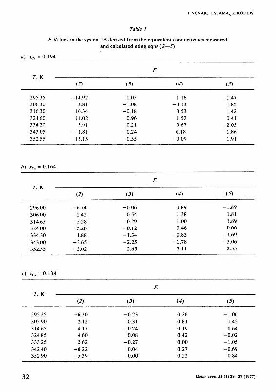
In order to decide which form of data interpretation is the most adequate and to be able to make a comparison with our former results [6] the differences between values of the equivalent conductivity calculated according to eqns (2—5) (Лса1с) and values of Л с х р are expressed as a relative error in per cent

Е = Л^~ЛелХк • 100. (6)

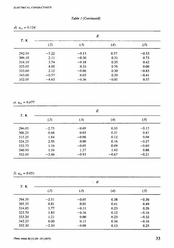
The comparison of results is summarized in Table ltf —/, where E values are listed for each series of xia at yrr =0.202 (system IB). The constants necessary to calculate the A according to eqns (2—5) are listed in Tables 2 and 3.

It was ascertained here and in our previous work, too (ycl- = 0.099, system IA) [6], that eqn (2) is entirely unsuitable to describe the system. The agreement between Л е х р and Л с а | с according to eqns (3—5) is fairly good, none of these three equations, however, gives E values appreciably lower than the remaining two equations.

The dependence on concentration

It is known that for the melt which is a mixture of the two pure ionic compounds Л can be calculated using Markov's relationship [13]. In our case it would be basically possible to calculate A in this way under the assumption that the

Chcm. zvesti 31 (1) 29—37 (1977) 31

J. NOVÁK. I. SLÁMA, Z. KODEJŠ

Table 1

E Values in the system IB derived from the equivalent conductivities measured and calculated using eqns (2—5)

а) xCa = 0.194

T к

295.35

306.30

316.30

324.60

334.20

343.05

352.55

(2)

-14.92

3.81

10.34

11.02

5.91

- 1.81

-13.15

U)

0.05

-1.08

-0.18

0.96

0.21

-0.24

-0.55

E

(4)

1.16

-0.13

0.53

1.52

0.67

0.18

-0.09

(Я

-1.47

1.85

1.42

0.41

-2.03

-1.86

1.91

b) xCa = 0.164

296.00

306.00

314.65

324.00

334.30

343.00

352.55

(2)

-6.74

2.42

5.28

5.26

1.88

-2.65

-3.02

(3)

-0.06

0.54

0.29

-0.12

-1.34

-2.25

2.65

E

(4)

0.89

1.38

1.00

0.46

-0.83

-1.78

3.11

(Я

-1.89

1.81

1.89

0.66

-1.69

-3.06

2.55

с) хСа = 0.138

T к

295.25

305.90

314.65

324.85

333.25

342.40

352.90

(2)

-6.30

2.12

4.17

4.60

2.62

-0.22

-5.39

(3)

-0.23

0.31

-0.24

0.08

-0.27

0.04

0.00

E

(4)

0.26

0.81

0.19

0.42

0.00

0.27

0.22

(S)

-1.06

1.42

0.64

-0.02

-1.05

-0.69

0.84

32 СЬет. zvesti 31 (1) 29—37 (1977)

ELECTRICAL CONDUCTIVITY

Table 1 (Continued)

d) xCa = 0.124

T к

292.50

306.10

314.10

325.05

333.60

343.00

352.05

(2)

-5.22

2.11

3.74

4.05

2.12

-0.57

-4.63

(3)

-0.13

-0.30

-0.18

0.33

-0.06

0.05

-0.36

E

(4)

0.57

0.31

0.35

0.76

0.30

0.39

-0.01

(S)

-0.53

0.73

0.42

0.00

-0.83

-0.41

0.57

e) xCil = 0.077

T, K

(2) (3) (4) (S)

296.05

306.25

315.25

324.25

333.75

340.95

352.45

-2.75

0.68

1.84

2.05

1.16

1.34

-3.46

0.05

0.03

0.08

0.00

0.05

1.27

0.93

0.33

0.31

0.12

0.16

0.09

1.43

-0.67

-0.17

0.41

0.04

-0.27

-0.60

0.88

-0.21

f) xCa = 0.051

T K

294.35

305.35

314.05

323.70

333.20

342.25

352.30

(2)

-2.51

0.81

1.77

1.83

1.21

0.00

-2.30

U)

-0.05

0.01

-0.11

-0.16

0.00

0.11

-0.09

E

(4)

0.38

0.41

0.23

0.12

0.23

0.34

0.13

(S)

-0.36

0.49

0.26

-0.16

-0.32

-0.16

0.25

CJiem. zvesti J l (1) 29—37 (1977) 33

J. NOVÁK. I. SLÁMA, Z. KODEJŠ

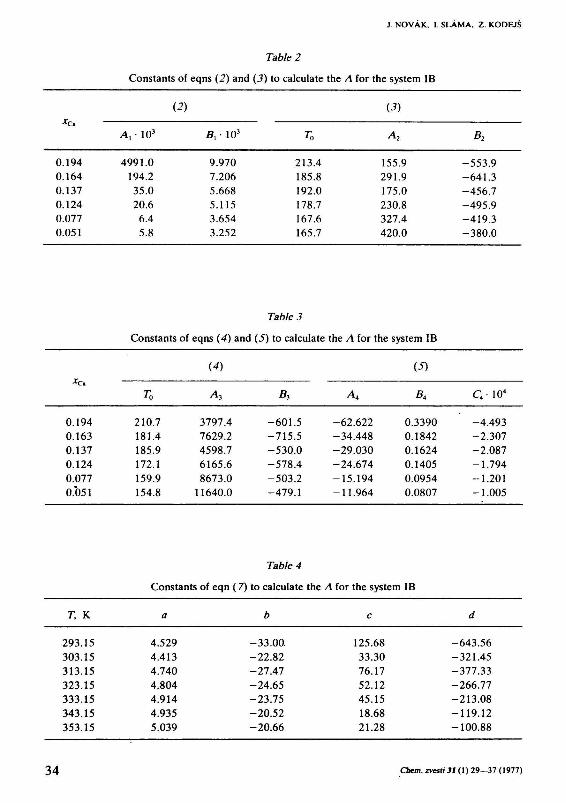
Table 2

Constants of eqns (2) and (3) to calculate the Л for the system IB

* C a

0.194 0.164

0.137 0.124 0.077 0.051

Ar 103

4991.0 194.2

35.0 20.6

6.4

5.8

(2)

Bx •103

9.970 7.206 5.668 5.115 3.654

3.252

To

213.4

185.8 192.0 178.7 167.6 165.7

(•?)

A2

155.9 291.9 175.0

230.8 327.4

420.0

B2

-553.9 -641.3 -456.7

-495.9 -419.3 -380.0

Table 3

Constants of eqns (4) and (5) to calculate the Л for the system IB

*c.

0.194 0.163 0.137 0.124 0.077

0.051

T0

210.7 181.4 185.9

172.1 159.9

154.8

(4)

A,

3797.4 7629.2 4598.7

6165.6

8673.0 11640.0

B,

-601.5 -715.5 -530.0 -578.4

-503.2 -479.1

A4

-62.622 -34.448 -29.030 -24.674

-15.194 -11.964

(S)

B4

0.3390 0.1842 0.1624

0.1405 0.0954 0.0807

C4 104

-4.493 -2.307 -2.087

-1.794 -1.201

-1.005

Table 4

Constants of eqn (7) to calculate the Л for the system IB

Г, к

293.15

303.15 313.15

323.15 333.15 343.15 353.15

а

4.529

4.413 4.740

4.804 4.914

4.935

5.039

b

-33.00. -22.82 -27.47

-24.65 -23.75 -20.52 -20.66

с

125.68 33.30 76.17

52.12 45.15 18.68 21.28

d

-643.56 -321.45 -377.33 -266.77 -213.08 -119.12 -100.88

3 4 Chcm. zvesti 31 (1) 29—37 (1977)

ELECTRICAL CONDUCTIVITY

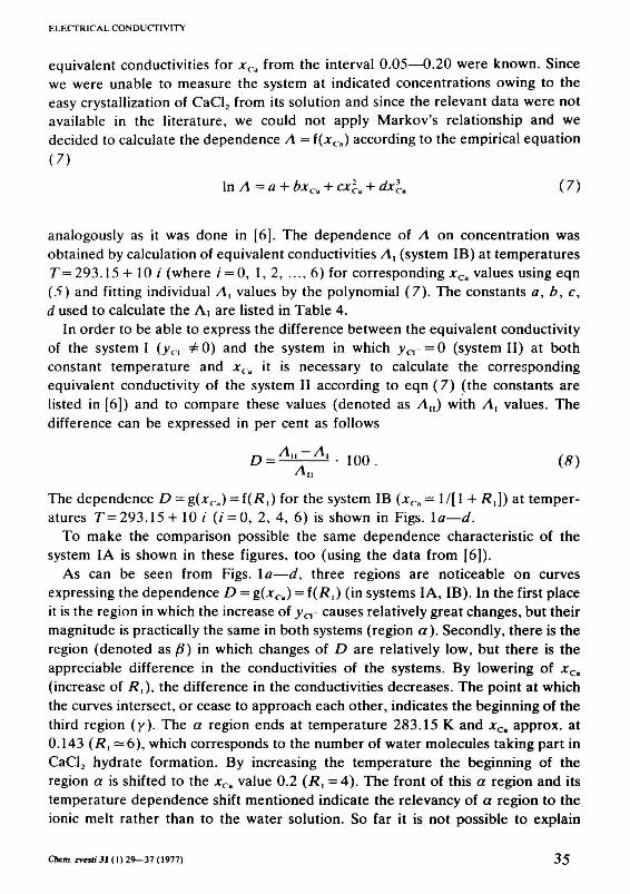
equivalent conductivities for xCa from the interval 0.05—0.20 were known. Since

we were unable to measure the system at indicated concentrations owing to the

easy crystallization of CaCl2 from its solution and since the relevant data were not

available in the literature, we could not apply Markov's relationship and we

decided to calculate the dependence A = i(xCa) according to the empirical equation

(7)

In Л = a + ЬхСа + cx2

Ca + dx\.a ( 7)

analogously as it was done in [6]. The dependence of Л on concentration was obtained by calculation of equivalent conductivities Л, (system IB) at temperatures Г=293.15 + 10 / (where / = 0, 1, 2, ..., 6) for corresponding xCa values using eqn (5) and fitting individual Л, values by the polynomial (7). The constants a, b, c, d used to calculate the Ai are listed in Table 4.

In order to be able to express the difference between the equivalent conductivity of the system I (ycl Ф0) and the system in which ycr = Q (system II) at both constant temperature and xCa it is necessary to calculate the corresponding equivalent conductivity of the system II according to eqn (7) (the constants are listed in [6]) and to compare these values (denoted as Л„) with Л, values. The difference can be expressed in per cent as follows

D = All-Al 1 0 0 w

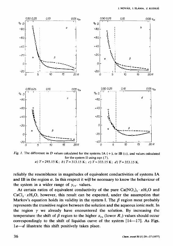
The dependence D = g(xcJ = f(Rl) for the system IB (xCa= 1/[1 + /?,]) at temper­atures T=293.15 + 10 / ( / = 0 , 2, 4, 6) is shown in Figs, la—d.

To make the comparison possible the same dependence characteristic of the system IA is shown in these figures, too (using the data from [6]).

As can be seen from Figs. \a—d, three regions are noticeable on curves expressing the dependence D = g(xCa) = i(Ri) (in systems I A, IB). In the first place it is the region in which the increase of yC]- causes relatively great changes, but their magnitude is practically the same in both systems (region a). Secondly, there is the region (denoted as ß) in which changes of D are relatively low, but there is the appreciable difference in the conductivities of the systems. By lowering of xCa

(increase of /?,), the difference in the conductivities decreases. The point at which the curves intersect, or cease to approach each other, indicates the beginning of the third region (y). The a region ends at temperature 283.15 К and x^ approx. at 0.143 (/?, = 6 ) , which corresponds to the number of water molecules taking part in CaCl2 hydrate formation. By increasing the temperature the beginning of the region a is shifted to the * C a value 0.2 (Ä, =4) . The front of this a region and its temperature dependence shift mentioned indicate the relevancy of a region to the ionic melt rather than to the water solution. So far it is not possible to explain

Chem. zvesti 31 (1) 29—37 (1977) 35

J. NOVÁK, 1. SLÁMA, Z. KODEJŠ

0.50 0.25 0.10 0.05 xCa 0.50 0.25 0.10 0.05 xCt

% D

+ 80

+ 60

+ 40

+20

0

-20

i i

i i

- \ i - \i

Л 1 1

^ír P

—+—

1

b

-

-

"*""*"" é 20 R 10 15 20R

0.500.25 0.10 005 xCa

% D

+ 80

+ 60

+ 40

-20

0

-20

-

-

-

+

u

p

^ s J r - + ~

c

I

-

-

- * I u I

10 15 20 R

%D

+60

+40

+20

0

-20

-40

0.50 025

1 ' !

+ ! 1 1

- . \ 1

, i

0.10 1

^ - - - 1 —

,

p — + —

0.05 1

d

-

-

i

10 15 20R

Fig. 1. The difference in D values calculated for the systems IA ( + ), or IB (o), and values calculated for the system II using eqn (7).

a) 7=293 .15 K; b) Г=313.15 К; с) Г=333.15 K; d) Г=353.15 К.

reliably the resemblance in magnitudes of equivalent conductivities of systems IA and IB in the region a. In this respect it will be necessary to know the behaviour of the system in a wider range of ycr values.

At certain ratios of equivalent conductivity of the pure Ca(N0 3 ) 2 • * Н 2 0 and CaCl2 • J : H 2 0 , however, this result can be expected, under the assumption that Markov's equation holds its validity in the system I. The ß region most probably represents the transitive region between the solution and the aqueous ionic melt. In the region у we already have encountered the solution. By increasing the temperature the shift of ß region to the higher хСл (lower Rx) values should occur correspondingly to the shift of liquidus curve of the system [14—17]. As Figs. \a—d illustrate this shift positively takes place.

36 Chem. zvestí 31 (1) 29—37 (1977)

ELECTRICAL CONDUCTIVITY

To explain the behaviour of systems IA and IB in the region a further information on changes of the equivalent conductivity in this relation at increasing ycr is necessary. This will be the subject of our next work.

References

1. Angell, С A., J. Phys. Chem. 70, 2793 (1966). 2. Moynihan, С. Т., J. Phys. Chem. 70, 3399 (1966).

3. Angell, C. A., J. Phys. Chem. 70, 3989 (1966). 4. Angell, С A., J. Phys. Chem. 69, 2137 (1965). 5. Angela С A. and Bressel, R. D., J. Phys. Chem. 76, 3244 (1972). 6. Novák, J., Sláma, I., and Kodejš, Z., Collect. Czech. Chem. Commun. 41, 2838 (1976). 7. Lind, J. E., Jr., Zwolenik, J. J., and Fuoss, R. M., J. Amer. Chem. Soc. 81, 1557 (1959). 8. Ying-Chech Chin and Fuoss, R. M., / Phys. Chem. 72, 4123 (1968). 9. Hoover, Т. В., J. Phys. Chem. 74, 2667 (1970).

10. Braunstein, J. and Robbins, G. D., J. Chem. Educ. 48, 52 (1971). 11. Angell, С A.. J. Phys. Chem. 70, 3988 (1966). 12. Bressel, R., Thesis. Purdue University, Lafayette, 1972. 13. Markov, B. F. and Shumina, L. A., Dok/. Akad. Nauk SSSR 110, 411 (1956). 14. Ehret, W. F., J. Amer. Chem. Soc. 54, 3126 (1932). 15. Vereshchagina, V. I., Derkacheva, V. N., Shulyak, L. F., and Zolotareva, L. V., Zh. Neorg. Khim.

18, 507 (1973). 16. Vereshchagina, V. I., Zolotareva, L. V., and Shulyak, L. F., Zh. Neorg. Khim. 14, 3390 (1969).

17. Ranaudo, C , Atti X" Congr. Int. Chim., Rome, 1939, Vol. 2; Gmelins Handbuch der anorgani­

schen Chemie, Calcium, Teil B, Lief. 2, 1957.

Translated by J. Majling

Chem. zvesú 31 (1) 29—37 (1977) 37