Modeling asymmetric distortion in multichannel radio frequency communication systems by Wonhoon Jang A dissertation submitted to the Graduate Faculty of North Carolina State University in partial fulfillment of the requirements for the Degree of Doctor of Philosophy Electrical Engineering Raleigh 2006 Approved By: Dr. Griff L. Bilbro Dr. W. Rhett Davis Dr. Michael B. Steer Dr. Douglas W. Barlage Chair of Advisory Committee
Transcript
Modeling asymmetric distortion in multichannel radio frequencycommunication systems
by
Wonhoon Jang
A dissertation submitted to the Graduate Faculty ofNorth Carolina State University
in partial fulfillment of therequirements for the Degree of
Doctor of Philosophy
Electrical Engineering
Raleigh
2006
Approved By:
Dr. Griff L. Bilbro Dr. W. Rhett Davis
Dr. Michael B. Steer Dr. Douglas W. BarlageChair of Advisory Committee
Abstract
JANG, WONHOON. Modeling asymmetric distortion in multichannel radio frequency
communication systems. (Under the direction of Dr. Michael B. Steer).
A multi-slice behavioral model is used to capture baseband memory effects in mul-
tichannel communication circuits and systems. The model is composed of two slices.
Each slice includes a static nonlinear function box and linear filters. The first slice
captures short-term memory effects and the second slice captures baseband memory
effects. A robust extraction procedure for the model is developed with a physically
realistic baseband slice. An efficient measurement method for the extraction is used.
A 2.4 GHz power amplifier is modeled as an example. The performance of the ex-
tracted model is verified by showing that it captures baseband effects when the power
amplifier is excited with a two-channel WCDMA signal. One of the advantages of
the model is that it can be used in various established simulation schemes such as en-
velope transient simulation and transient (time-marching or SPICE-like) simulation.
The model is shown to be compatible with both. In the transient simulation, the
model supports the use of a much lower carrier frequency. This results in enhanced
computational efficiency and the same results are achieved. This opens up a new con-
tribution for RF system simulation where complex signals comprise of signals that can
be of general form including signals that cannot be represented as modulated carriers.
While envelope transient simulation is restricted to slowly modulated carriers, there
is no restriction on the type of drive signal so that single tone, multi-tone, CDMA,
chirp and noise signals can be combined.
ii
This dissertation is dedicated to my son, Inyoung A. Jang, and my wife, Eunjung
Park, and also to my parents in Korea . . .
iii
Biography
Wonhoon Jang received the B.S. degree in electronics from Kyungpook National
University in Daegu, Korea, in 1997. He is presently working toward Ph.D. degree
in electrical engineering at North Carolina State University in Raleigh. From 1997
to 1999, he was with LG Precision Co., Kumi, Korea, where he was involved with
military radios. His current research interests include nonlinear RF/microwave system
analysis and modeling.
iv
Acknowledgements
I would like to thank Dr. Michael B. Steer for serving as my academic advisor and sup-
porting me during my study. His great help made it possible for me to come this far. I
also like to thank Dr. Griff L. Bilbro, Dr. W. Rhett Davis and Dr. Douglas W. Barlage
for serving on my committee and would like to thank Dr. Jon-Paul Maria for serving as
a graduate representative. Many thanks go to Dr. Kevin Gard, to Dr. Steer’s present
and past graduate students, Aaron Walker, Frank Heart, Jayesh Nath, Mark Buff,
Nikhil Kriplani, Ramya Mohan, Sonali Luniya, and to Dr. Wael Fathelbab for sharing
valuable talks and fun. Special thanks go to Stephen Bruss for sharing his harmonic
balance codes in MATLAB at www.uaf.edu/asgp/spbruss/other/em. I extensively
used his code in my envelope transient codes attached in Appendix A.
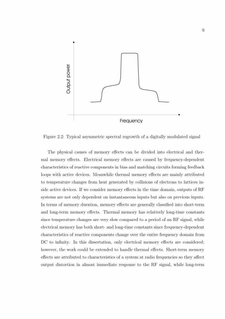
2.2 Typical asymmetric spectral regrowth of a digitally modulated signal 92.3 Frequency-dependent small-signal gain and saturated gain . . . . . . 112.4 Frequency spectra: (a) a single-tone input swept in frequency and
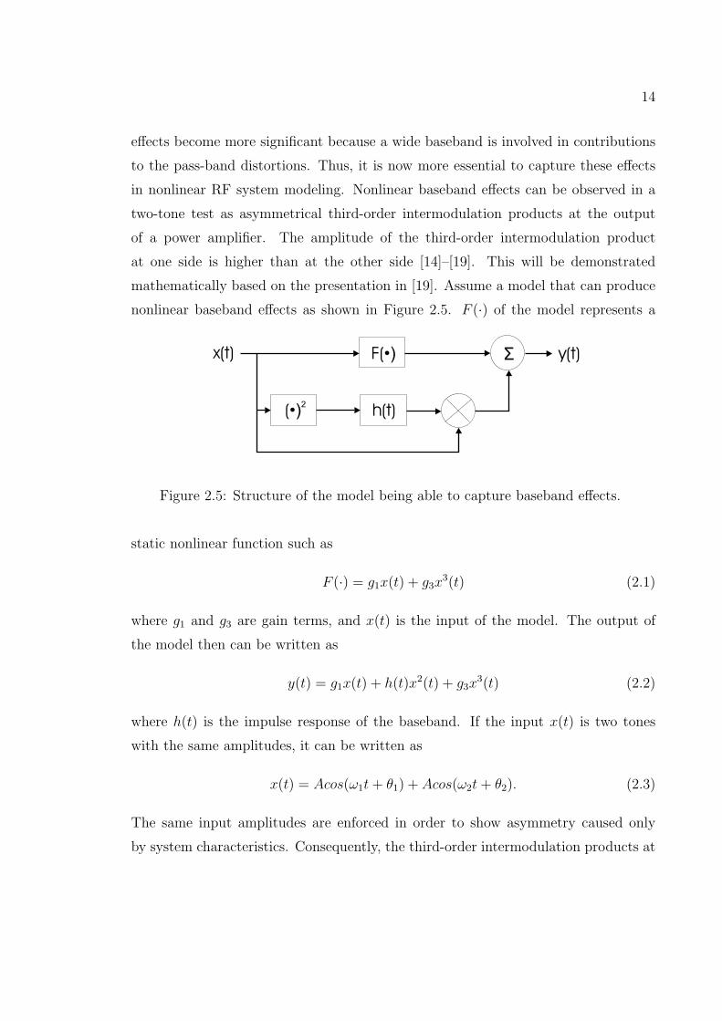
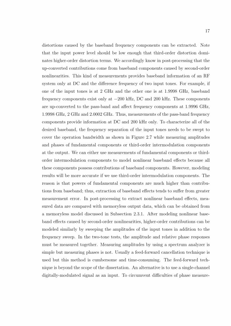
amplitude; and (b) the corresponding output. . . . . . . . . . . . . . 122.5 Structure of the model being able to capture baseband effects. . . . . 142.6 Demonstration of the asymmetry mechanism based on (2.4) and (2.5). 152.7 Frequency spectra of (a) a two tone input swept in frequency and
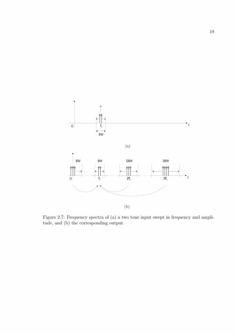
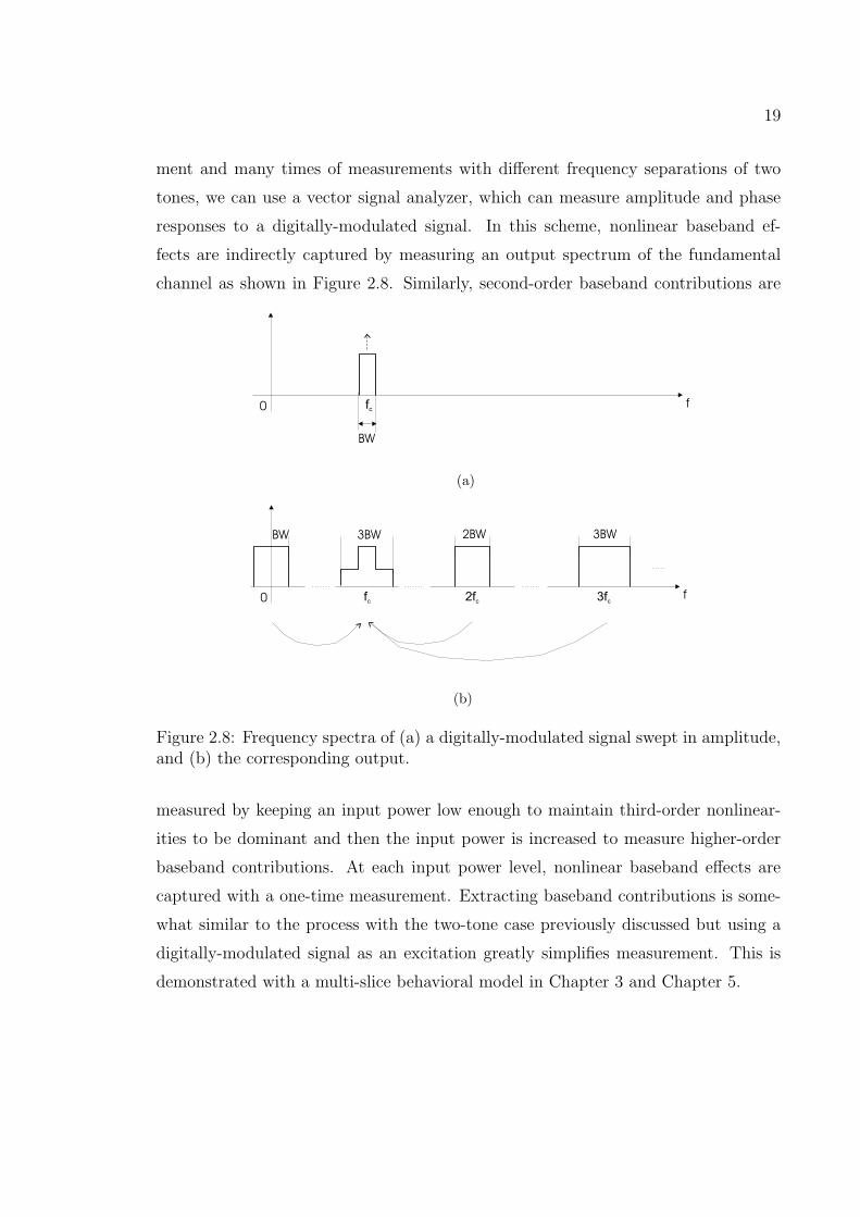
amplitude, and (b) the corresponding output. . . . . . . . . . . . . . 182.8 Frequency spectra of (a) a digitally-modulated signal swept in ampli-
tude, and (b) the corresponding output. . . . . . . . . . . . . . . . . 192.9 Structure of bandpass-type behavioral model . . . . . . . . . . . . . 212.10 Structure of the memory polynomial model . . . . . . . . . . . . . . 252.11 System identification of the memory polynomial model . . . . . . . . 272.12 Sequential implementation of the memory polynomial model . . . . . 282.13 Structure of the Wiener-Hammerstein model . . . . . . . . . . . . . 302.14 AM-PM responses of the Wiener-Hammerstein model . . . . . . . . 322.15 AM-AM responses of the Wiener-Hammerstein model . . . . . . . . 342.16 Partition of a circuit in harmonic balance . . . . . . . . . . . . . . . 362.17 Frequency domain representations of a single-channel digitally-modulated
signal: (a) its spectrum; (b) its representation as a phasor with am-plitude and phase varying slowly in time; (c) envelope signal; (d) thephasor presentation of the envelope; and (e) its windowed spectrum ofthe modulated RF signal in (a). . . . . . . . . . . . . . . . . . . . . 40
2.18 (a) spectrum of the electrical variable; (b) its transfer function; (c)down-converted spectrum and (d) down-converted transfer function. 41
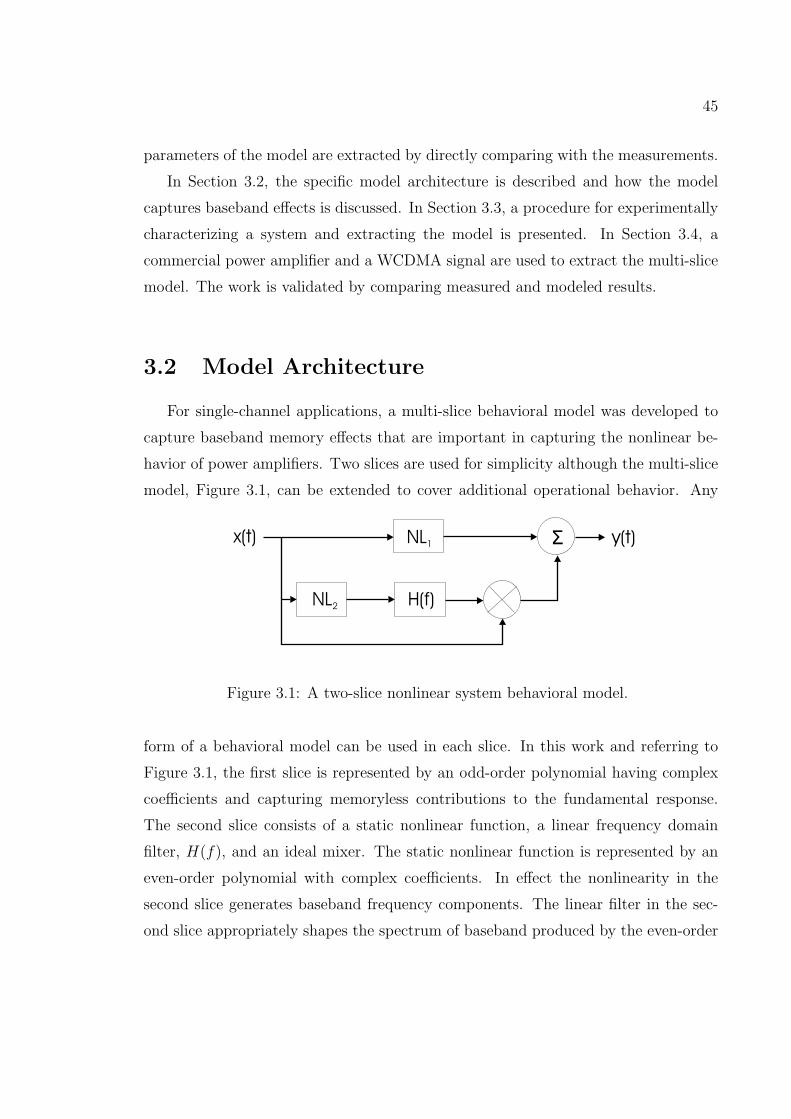
3.1 A two-slice nonlinear system behavioral model. . . . . . . . . . . . . 45
viii
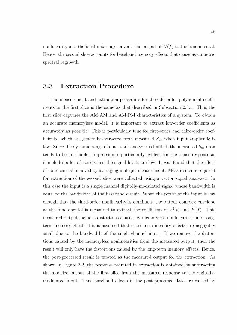
3.2 A block diagram showing extraction procedure of the two-slice nonlin-ear system behavioral model. . . . . . . . . . . . . . . . . . . . . . . 47
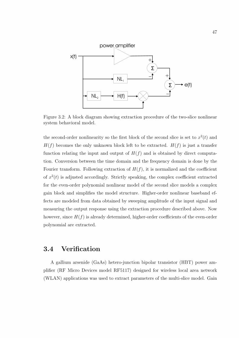
3.3 Measured and modelled AM-AM characteristics of the amplifier at2.5 GHz. (The measured and modelled characteristics overlap.) . . . 48
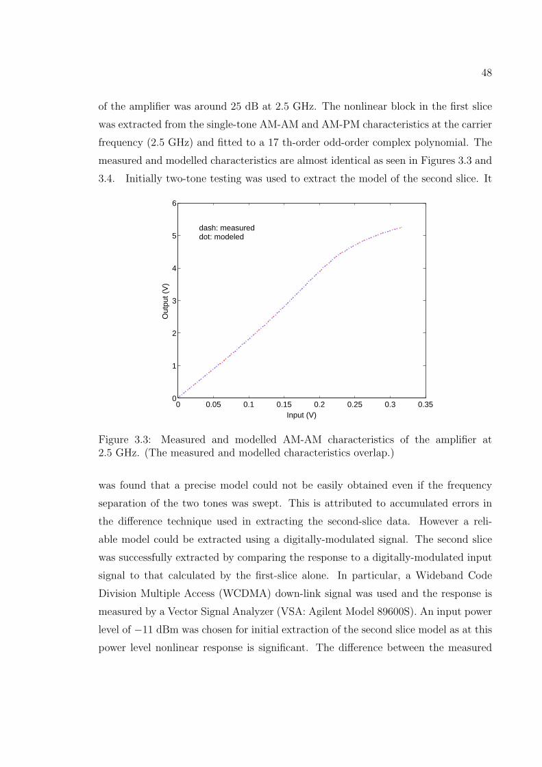
3.4 Measured and modelled AM-PM characteristics of the amplifier at2.5 GHz. (The measured and modelled characteristics overlap.) . . . 49
3.5 Normalized magnitude of H(f) which is used directly in the model. . 503.6 Modelled phase characteristics of H(f) which is used directly in the
asymmetry and comparison of the modeled and measured results. . . 523.10 Asymmetries of measured and modelled spectral regrowth. . . . . . . 533.11 Real part of the modelled and measured output complex envelopes in
the time domain. . . . . . . . . . . . . . . . . . . . . . . . . . . . . . 543.12 Imaginary part of the modelled and measured output complex en-
velopes in the time domain. . . . . . . . . . . . . . . . . . . . . . . . 543.13 Output frequency spectra of the model with and without memory, and
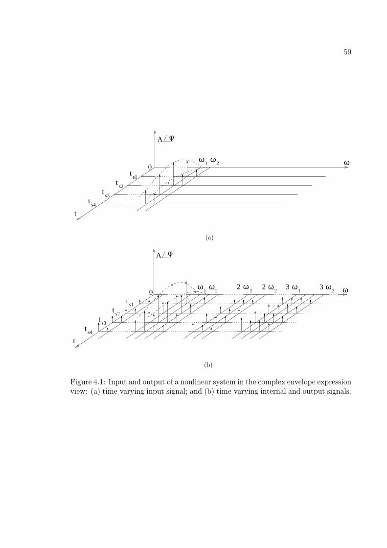
4.1 Input and output of a nonlinear system in the complex envelope expres-sion view: (a) time-varying input signal; and (b) time-varying internaland output signals. . . . . . . . . . . . . . . . . . . . . . . . . . . . 59
4.2 Spectrum of signals in a nonlinear system considered in MET analysis:(a) spectra of source signals; and (b) spectra of internal circuit andoutput signals. . . . . . . . . . . . . . . . . . . . . . . . . . . . . . . 61
4.3 Input and output spectra of the PCS amplifier with an IS-95 signalmodelled using the time-varying HB and ET method. Center frequencyis 1.9 GHz. (The output spectra of the time-varying HB and ET over-lap.) . . . . . . . . . . . . . . . . . . . . . . . . . . . . . . . . . . . . 65
4.4 Magnitude differences between lower and upper IM3 products of thePCS amplifier with two tones separated by 200 KHz. . . . . . . . . . 66
4.5 Input and output spectra of the modified PCS amplifier with an IS-95signal modelled using the time-varying HB and ET method. Centerfrequency is 1.9 GHz. . . . . . . . . . . . . . . . . . . . . . . . . . . 66
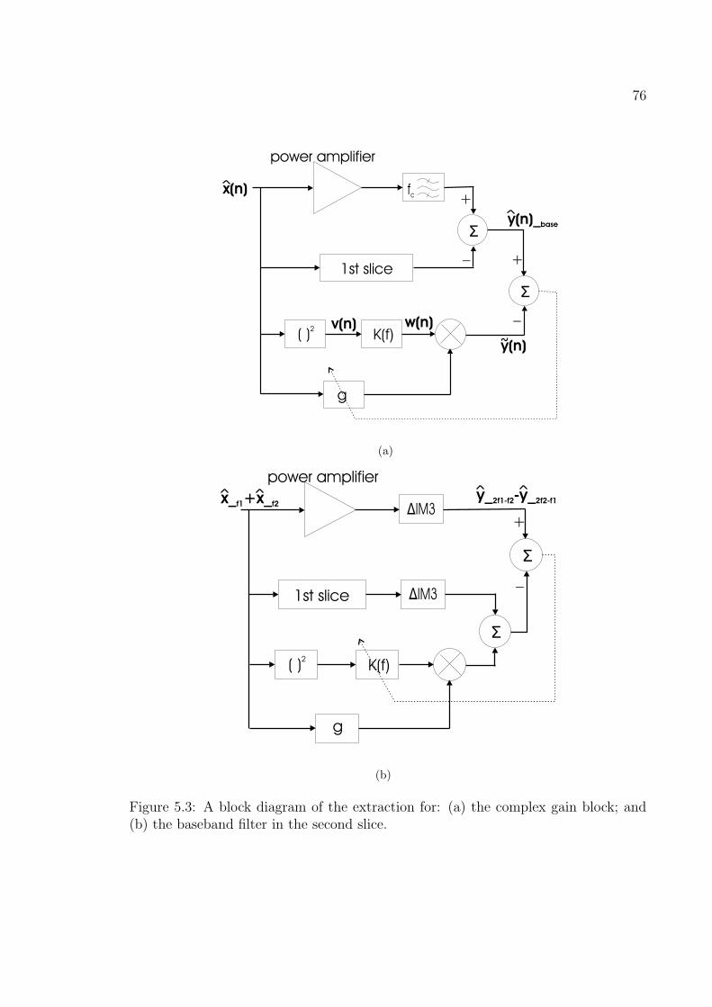
5.2 A block diagram of the extraction for the linear filters in the first slice. 745.3 A block diagram of the extraction for: (a) the complex gain block; and
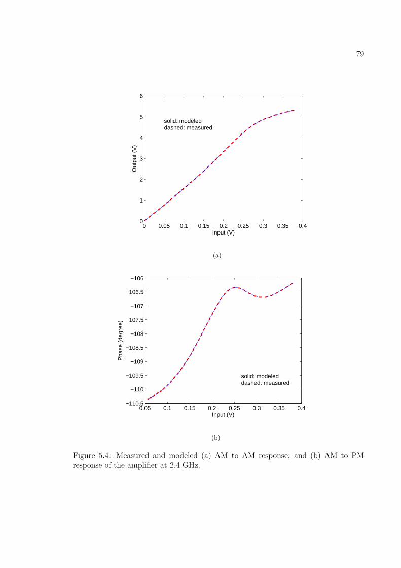
(b) the baseband filter in the second slice. . . . . . . . . . . . . . . . 765.4 Measured and modeled (a) AM to AM response; and (b) AM to PM
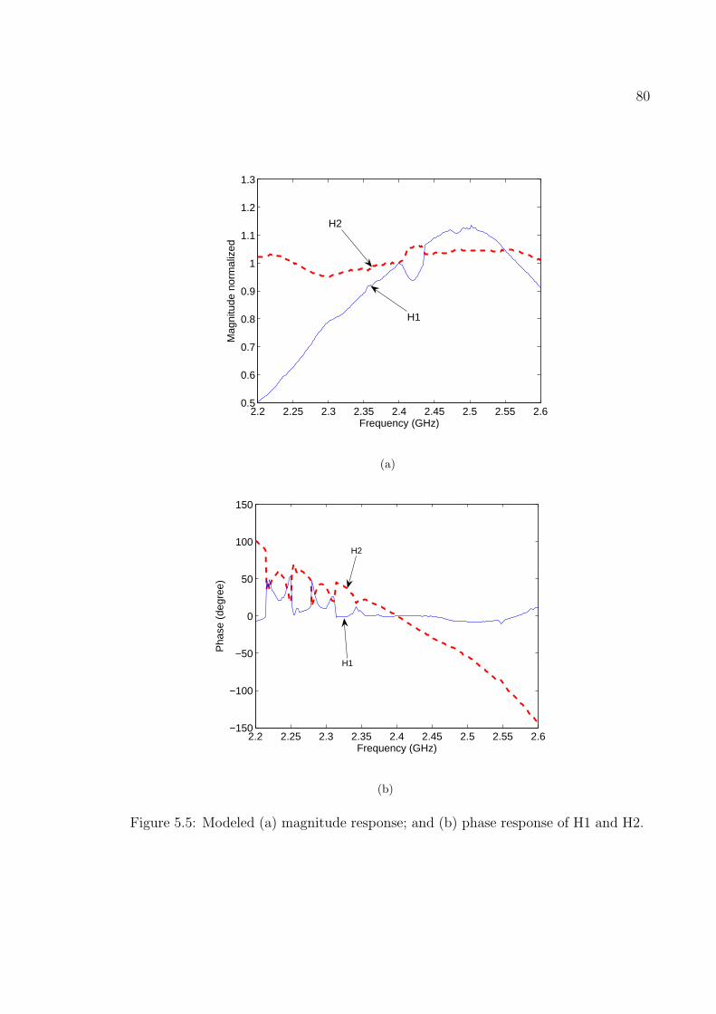
response of the amplifier at 2.4 GHz. . . . . . . . . . . . . . . . . . . 795.5 Modeled (a) magnitude response; and (b) phase response of H1 and H2. 805.6 (a) Measured AM-AM responses; and (b) modeled AM-AM responses
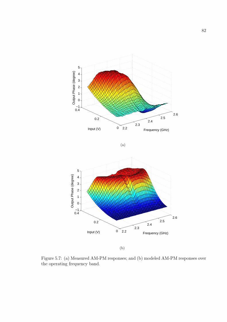
over the operating frequency band. . . . . . . . . . . . . . . . . . . . 815.7 (a) Measured AM-PM responses; and (b) modeled AM-PM responses
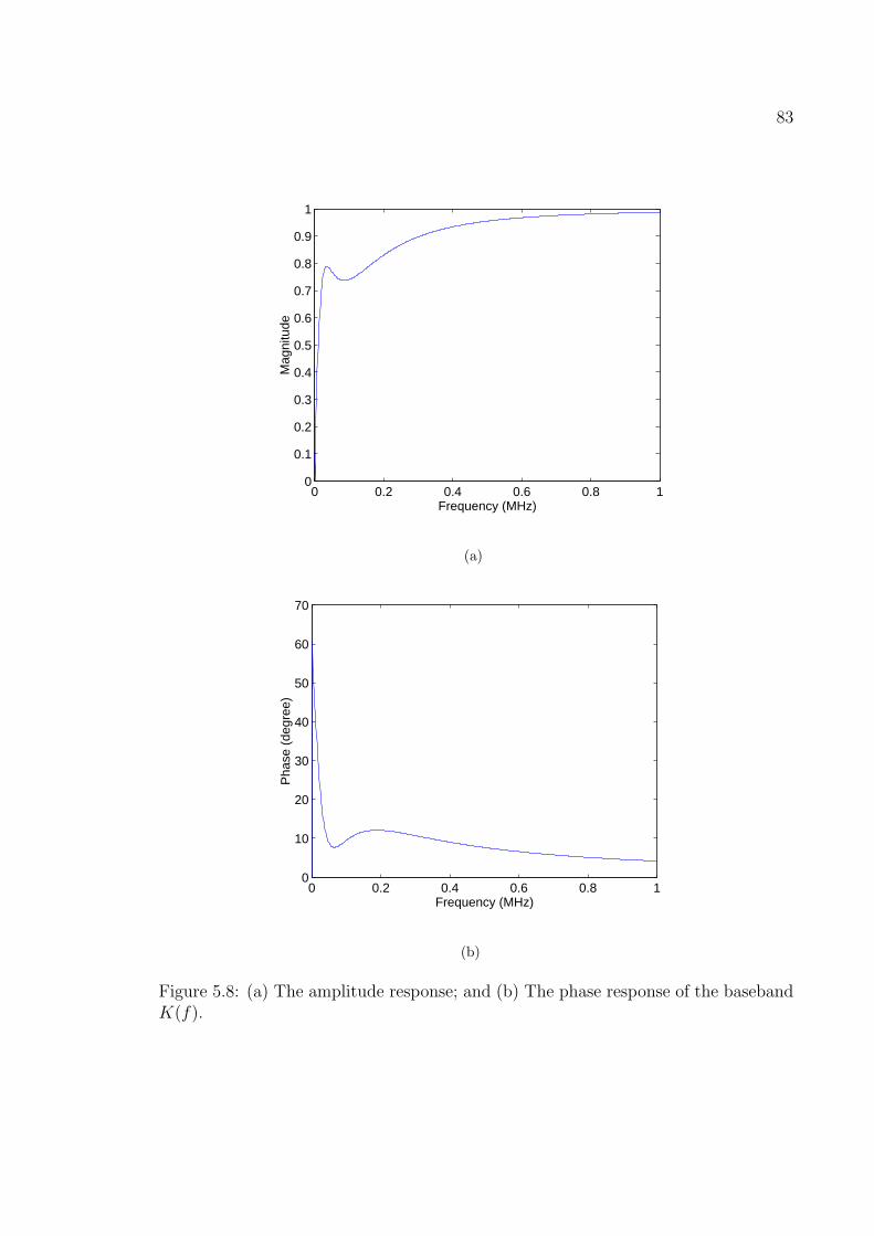
over the operating frequency band. . . . . . . . . . . . . . . . . . . . 825.8 (a) The amplitude response; and (b) The phase response of the base-
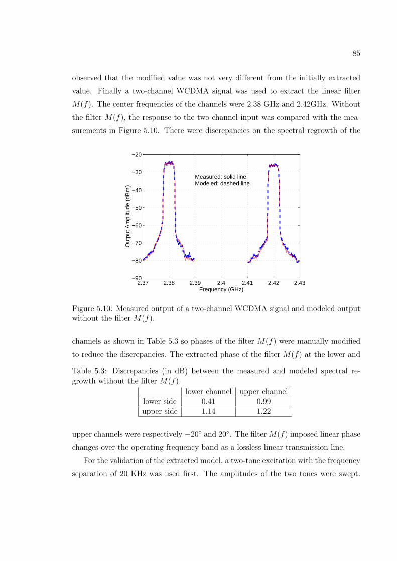
band K(f). . . . . . . . . . . . . . . . . . . . . . . . . . . . . . . . . 835.9 Measured and modeled magnitude of ∆IM3 as a function of frequency
without the filter M(f). . . . . . . . . . . . . . . . . . . . . . . . . . 855.11 Modeled phase response of H1 and H2. . . . . . . . . . . . . . . . . 865.12 (a) The modeled amplitude responses with and without baseband ef-
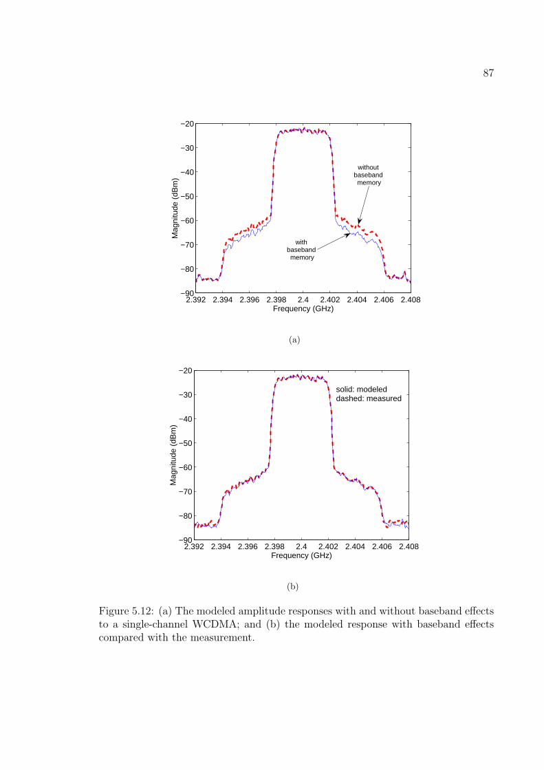
fects to a single-channel WCDMA; and (b) the modeled response withbaseband effects compared with the measurement. . . . . . . . . . . 87
5.13 (a) The modeled phase responses with and without baseband effectsto a single-channel WCDMA; and (b) the modeled response with base-band effects compared with the measurement. . . . . . . . . . . . . . 89
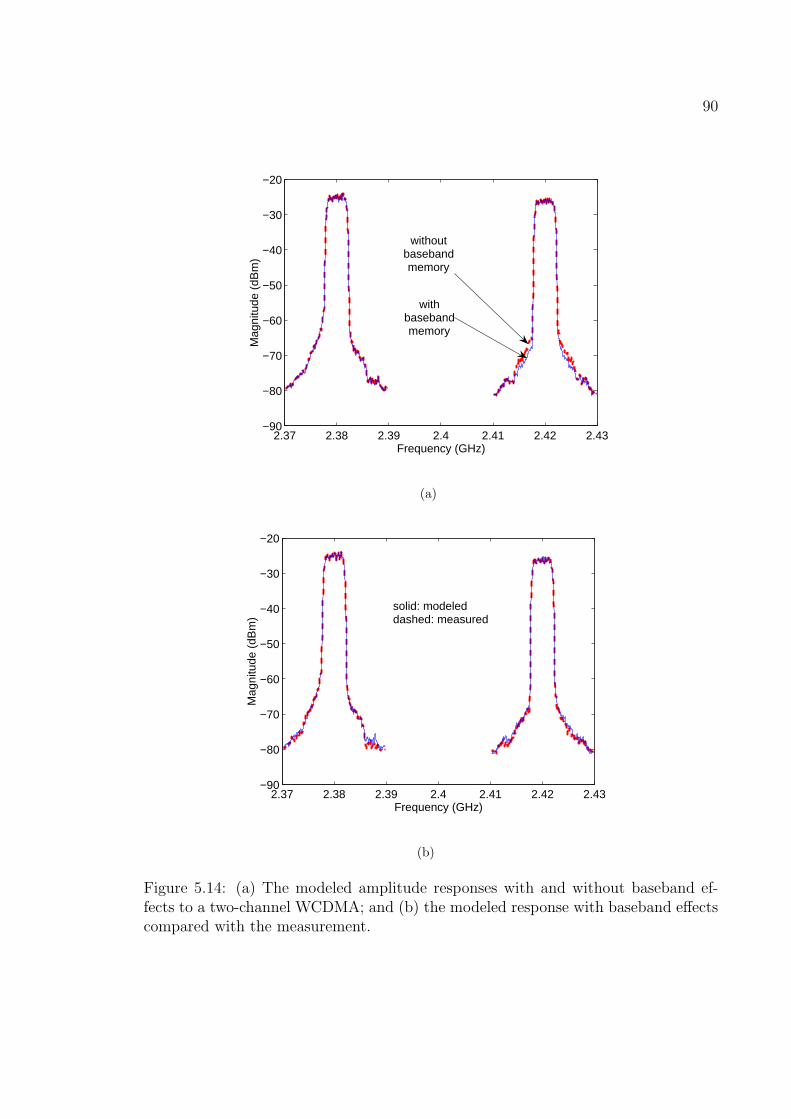
5.14 (a) The modeled amplitude responses with and without baseband ef-fects to a two-channel WCDMA; and (b) the modeled response withbaseband effects compared with the measurement. . . . . . . . . . . 90
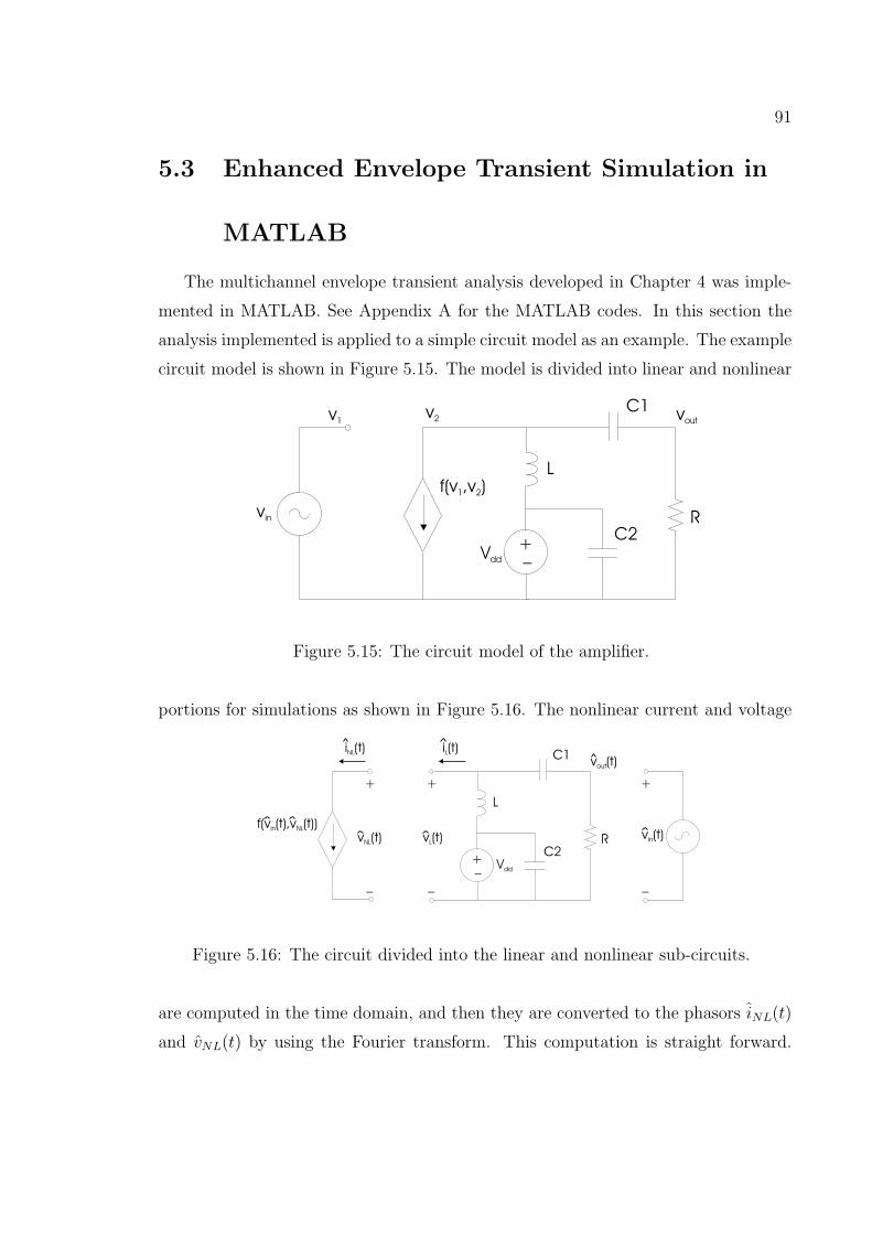
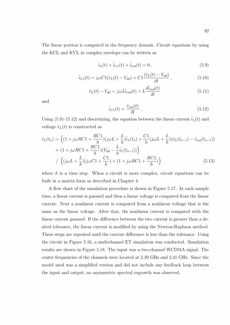
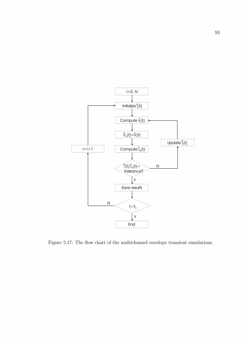
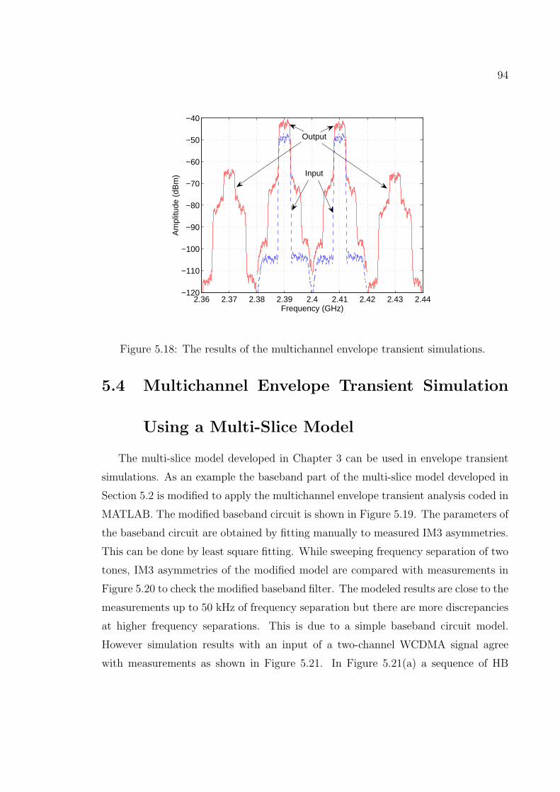
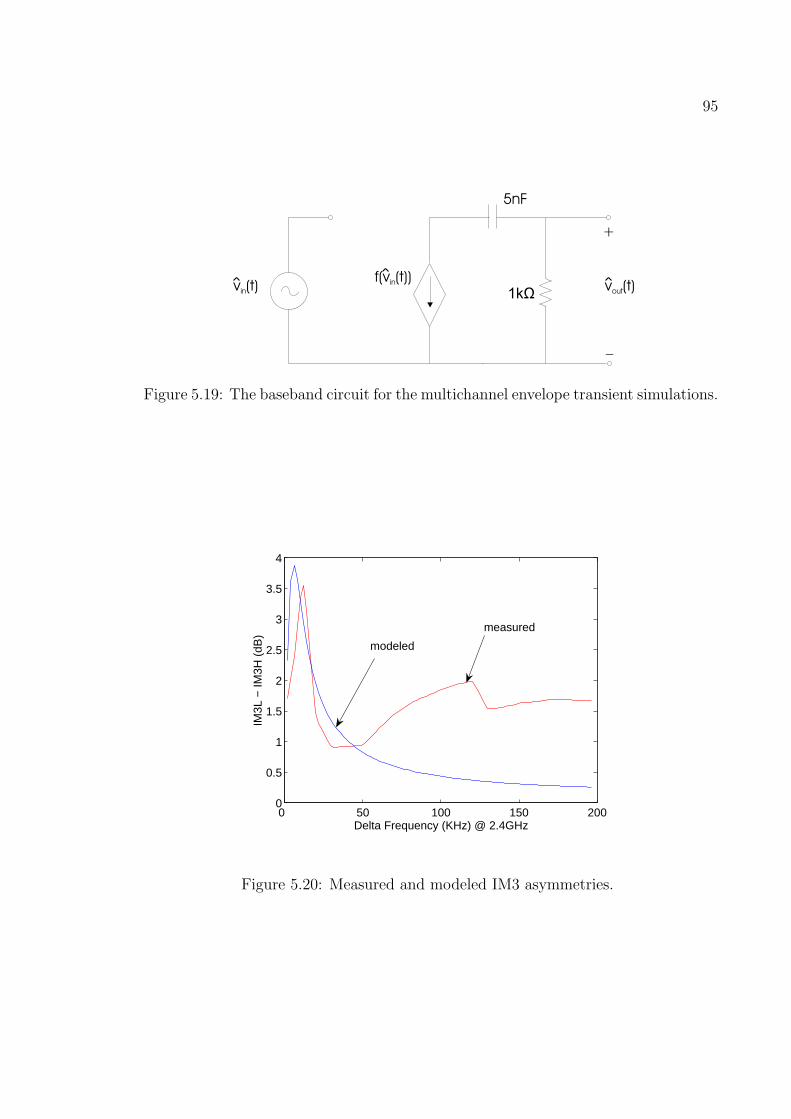
5.15 The circuit model of the amplifier. . . . . . . . . . . . . . . . . . . . 915.16 The circuit divided into the linear and nonlinear sub-circuits. . . . . 915.17 The flow chart of the multichannel envelope transient simulations. . 935.18 The results of the multichannel envelope transient simulations. . . . 945.19 The baseband circuit for the multichannel envelope transient simula-
fects to a two-channel WCDMA; and (b) the modeled response withbaseband effects compared with the measurement. . . . . . . . . . . 96
x
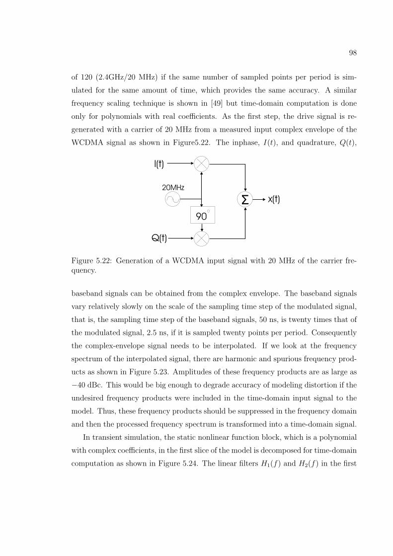
5.22 Generation of a WCDMA input signal with 20 MHz of the carrierfrequency. . . . . . . . . . . . . . . . . . . . . . . . . . . . . . . . . . 98
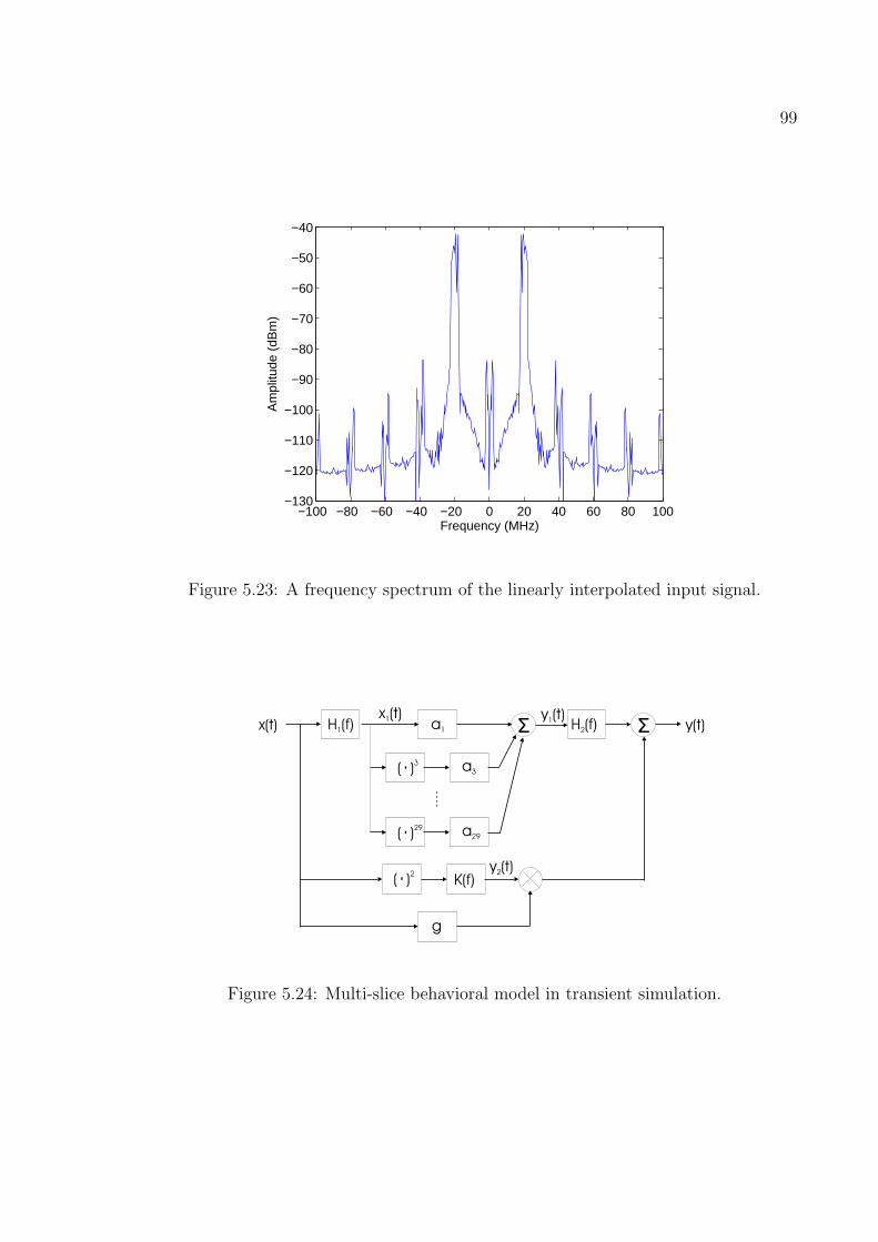
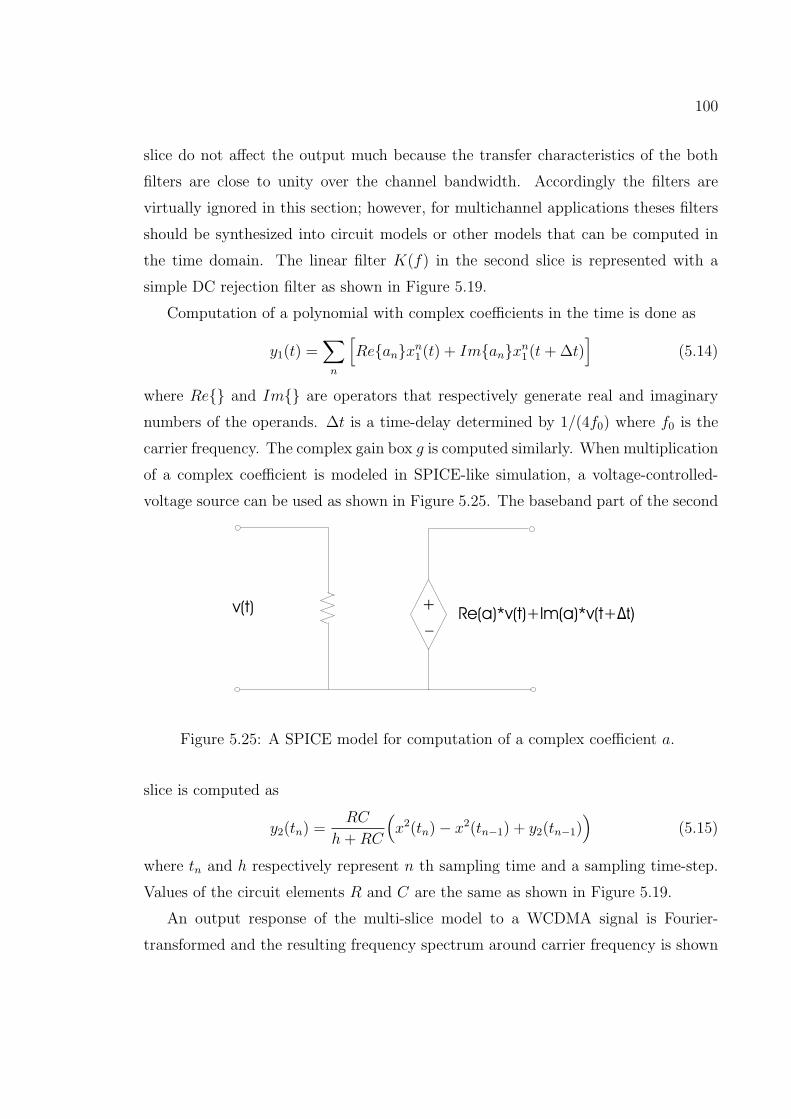
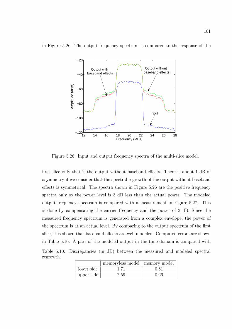
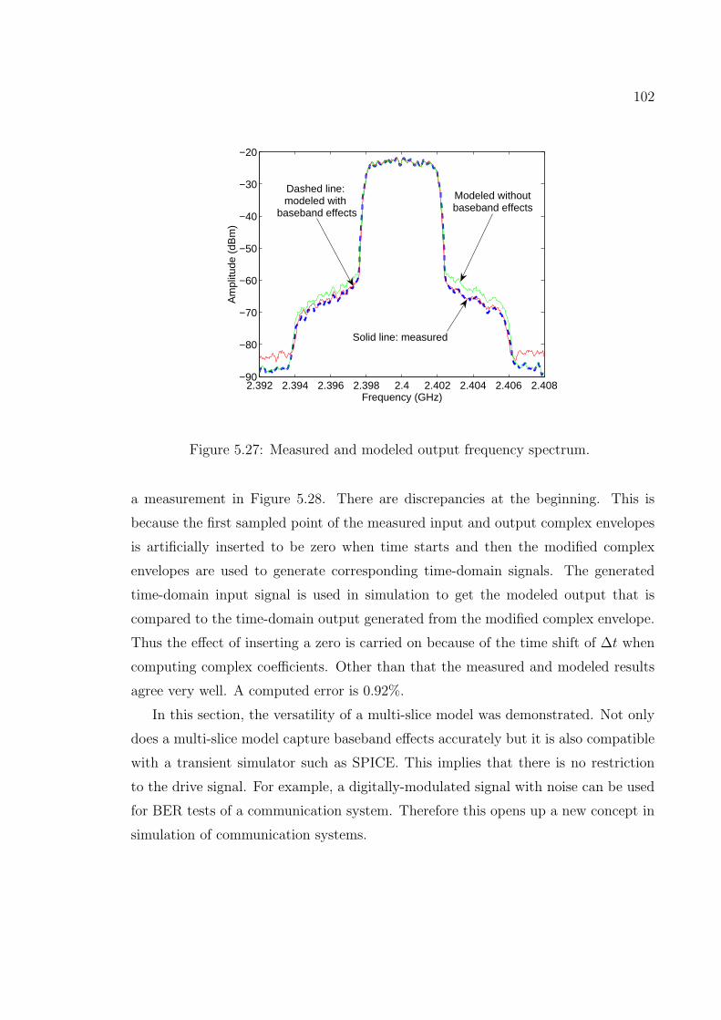
5.23 A frequency spectrum of the linearly interpolated input signal. . . . 995.24 Multi-slice behavioral model in transient simulation. . . . . . . . . . 995.25 A SPICE model for computation of a complex coefficient a. . . . . . 1005.26 Input and output frequency spectra of the multi-slice model. . . . . 1015.27 Measured and modeled output frequency spectrum. . . . . . . . . . 1025.28 A part of the modeled and measured time-domain signal. . . . . . . 103
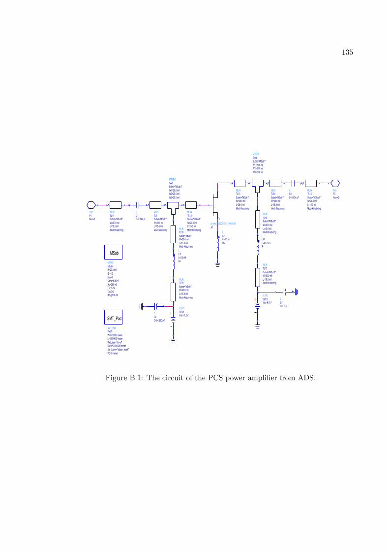
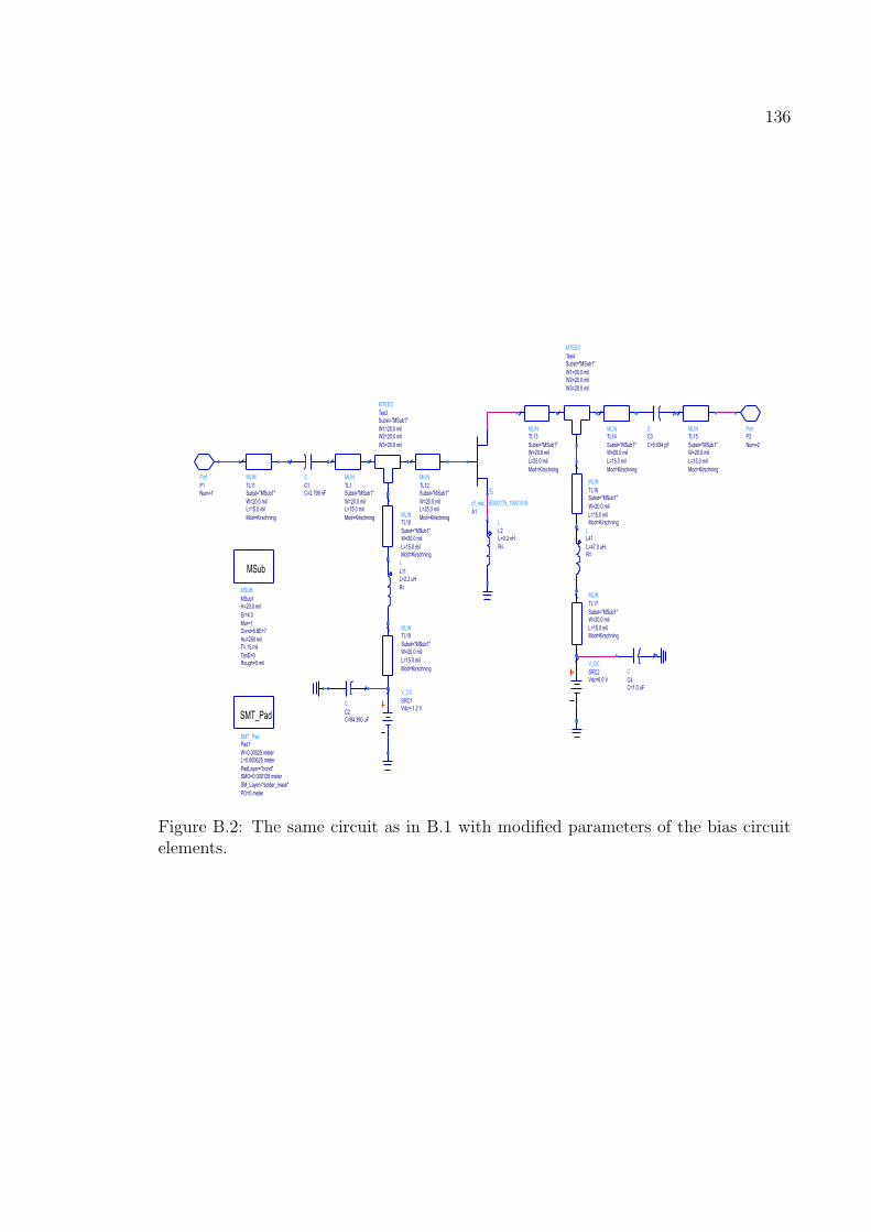
B.1 The circuit of the PCS power amplifier from ADS. . . . . . . . . . . 135B.2 The same circuit as in B.1 with modified parameters of the bias circuit
5.1 The extracted values of the complex gain g . . . . . . . . . . . . . . . 785.2 The extracted poles and zeros of the baseband filter K(f) . . . . . . 845.3 Discrepancies (in dB) between the measured and modeled spectral re-
growth without the filter M(f). . . . . . . . . . . . . . . . . . . . . . 855.4 Discrepancies (in dB) between the measured and modeled spectral re-
growth. . . . . . . . . . . . . . . . . . . . . . . . . . . . . . . . . . . 865.5 Discrepancies between the measured and modeled phase. . . . . . . . 885.6 Discrepancies (in dB) between the measured and modeled (without
baseband effects) spectral regrowth. . . . . . . . . . . . . . . . . . . . 885.7 Discrepancies (in dB) between the measured and modeled (with base-
band effects) spectral regrowth. . . . . . . . . . . . . . . . . . . . . . 885.8 Discrepancies (in dB) between the measured and modeled (without
baseband effects) spectral regrowth. . . . . . . . . . . . . . . . . . . . 975.9 Discrepancies (in dB) between the measured and modeled (with base-
band effects) spectral regrowth. . . . . . . . . . . . . . . . . . . . . . 975.10 Discrepancies (in dB) between the measured and modeled spectral re-
By using (2.6) and (2.15), the bandpass outputs of the memoryless nonlinear model
for multichannel applications can be obtained. For example, the bandpass output
around ω1 is computed when the exponent of the first exponential function in (2.15)
is ±1 and the exponents of the other exponential functions are zeros.
2.3.2 Memory Polynomial Model
One of the recent behavioral models able to capture memory effects of RF power
amplifiers is the memory polynomial model [29]–[31]. The model is regarded as a trun-
cation of the general Volterra series [32] since it contains significantly fewer Volterra
25
kernels. This is an efficient way in terms of computation and modeling. In another
perspective, the memory polynomial model being used to model a nonlinear system
with memory corresponds to the adaptive delay filter [33] being used to model a linear
system with memory. Instead of linear gain blocks in the adaptive delay filter, static
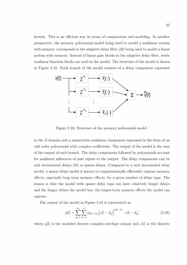
nonlinear function blocks are used in the model. The structure of the model is shown
in Figure 2.10. Each branch of the model consists of a delay component expressed
Ó
Z-d1 F(·)
1
F(·)2
F (·)m
Z-d2
Z-dm
x[l]
y[l]
Figure 2.10: Structure of the memory polynomial model
in the Z-domain and a memoryless nonlinear component expressed in the form of an
odd order polynomial with complex coefficients. The output of the model is the sum
of the output of each branch. The delay components followed by polynomials account
for nonlinear influences of past inputs to the output. The delay components can be
unit incremental delays [34] or sparse delays. Compared to a unit incremental delay
model, a sparse delay model is known to computationally efficiently capture memory
effects, especially long term memory effects, for a given number of delay taps. The
reason is that the model with sparse delay taps can have relatively longer delays
and the longer delays the model has, the longer-term memory effects the model can
capture.
The output of the model in Figure 2.10 is represented as
y[l] =m∑
q=1
n∑
k=1
a2k−1,q
∣∣∣x[l − dq]∣∣∣2(k−1)
· x[l − dq] (2.16)
where y[l] is the modeled discrete complex-envelope output and x[l] is the discrete
26
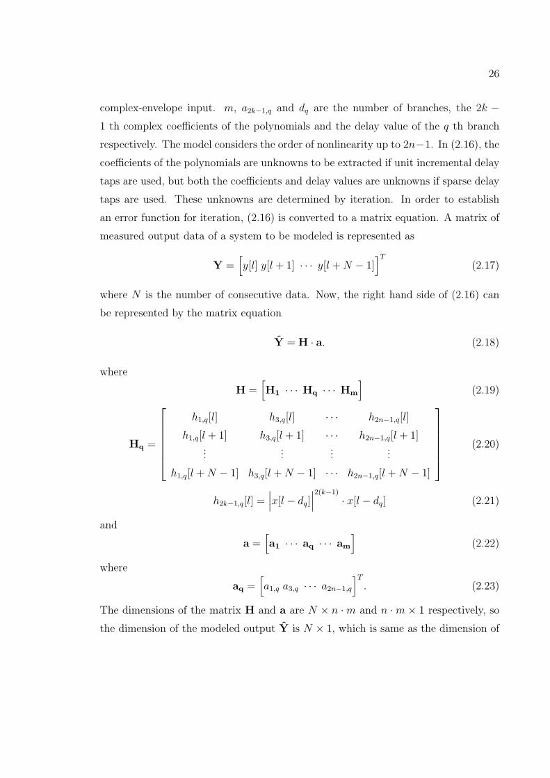
complex-envelope input. m, a2k−1,q and dq are the number of branches, the 2k −1 th complex coefficients of the polynomials and the delay value of the q th branch
respectively. The model considers the order of nonlinearity up to 2n−1. In (2.16), the
coefficients of the polynomials are unknowns to be extracted if unit incremental delay
taps are used, but both the coefficients and delay values are unknowns if sparse delay
taps are used. These unknowns are determined by iteration. In order to establish
an error function for iteration, (2.16) is converted to a matrix equation. A matrix of
measured output data of a system to be modeled is represented as
Y =[y[l] y[l + 1] · · · y[l + N − 1]
]T
(2.17)
where N is the number of consecutive data. Now, the right hand side of (2.16) can
be represented by the matrix equation
Y = H · a. (2.18)
where
H =[H1 · · · Hq · · · Hm
](2.19)
Hq =
h1,q[l] h3,q[l] · · · h2n−1,q[l]
h1,q[l + 1] h3,q[l + 1] · · · h2n−1,q[l + 1]...
......
...
h1,q[l + N − 1] h3,q[l + N − 1] · · · h2n−1,q[l + N − 1]
(2.20)
h2k−1,q[l] =∣∣∣x[l − dq]
∣∣∣2(k−1)
· x[l − dq] (2.21)
and
a =[a1 · · · aq · · · am
](2.22)
where
aq =[a1,q a3,q · · · a2n−1,q
]T
. (2.23)
The dimensions of the matrix H and a are N × n ·m and n ·m × 1 respectively, so
the dimension of the modeled output Y is N × 1, which is same as the dimension of
27
the measured output Y. An error function is formulated as
E = Y − Y (2.24)
= Y −H · a (2.25)
=[e[l] e[l + 1] · · · e[l + N − 1]
]T
(2.26)
where e[l] is a difference vector between the measured and modeled datum at the sam-
ple time l. The accuracy of extracted parameters, the delay values and the coefficients
of the polynomials, can be quantified as the rms value of the error E:
rmse =
(1
N
N−1∑
k=0
∣∣∣e[l + k]∣∣∣2)1/2
. (2.27)
The parameters are determined such that the rms error is minimized. A block diagram
of the system identification is shown in Figure 2.11. For the unit incremental delay
Nonlinear RF System
a dand
Demodulator DemodulatorI
QYH Y
Ó
I
Q
+
_
E
RF Input RF Output
Figure 2.11: System identification of the memory polynomial model
model, the delay value matrix, d = [d1 d2 · · · dm], are fixed as d = [1 2 · · · m], so the
parameters to be extracted are the coefficients of the polynomials, a. The coefficients
can be relatively easily determined by iteration, such as the Newton-Raphson method.
However, the delay values are also unknowns for the sparse delay model in addition
to the coefficients of the polynomials. The delay values and coefficients cannot be
extracted by iteration at the same time. The reason is that an expected delay value
needa to be a natural number; however, the error values from (2.24) are complex
numbers and the resulting Jacobian matrix is also complex so that iterative fitting
28
generates complex delay values. In references [33] and [35] the parameters of the
model were determined by sequential implementation in which the first branch of the
model was extracted and then the second was done and so on as shown in Figure 2.12.
In the sequential implementation there are two loops of iteration for each branch.
Ó
Z-d1 F(·)
1
F(·)2
F (·)m
Z-d2
Z-dm
x[l] Nonlinear RF System
Ó
Ó
+
_
+
_
+
_
e [l]1
e [l]2
e [l]m
Figure 2.12: Sequential implementation of the memory polynomial model
The inner loop is for the coefficients of the polynomials and the outer loop is for
the sparse delay taps. Up to a certain maximum delay, the optimum coefficients
are extracted iteratively while delay values are incrementally changed, and then the
optimum delay values and coefficients are chosen. Usually the first delay value is zero
due to dominance of the memoryless portion over the memory portion of a power
amplifier.
A memory polynomial model can capture memory effects but there are two aspects
to be considered on modeling memory effects. First, the model is not suitable for
capturing short-term memory effects since a baseband-like complex-envelope signal
is used to extract parameters of the model and usually time constants of short-term
memory effects are shorter than a sampling period of the complex envelope. The
other aspect of the model is that it can capture long-term memory effects; however,
it only captures some of the actual memory effects of a power amplifier. The reason
is that each branch of the model has single constant delay component so it captures
29
memory effects caused from characteristics of the amplifier at only a single frequency.
As to an incremental unit delay model, it could rigorously capture long-term memory
effects of a system if the sampling frequency of the input data were high enough to
account for long-term memory effects with a relatively short-time constant and the
model had a sufficient number of branches to account for long-term memory effects
with a relatively long-time constant. The advantage of the sparse delay model is
its simplicity but it is not suitable for modeling memory effects when an amplifier
exhibits a lot of variation of characteristics over a relatively narrow frequency band,
especially baseband. A relatively narrow frequency band is very common in practical
amplifiers. Therefore, optimum parameter extraction of a memory polynomial model
is not only difficult but also likely to be dependent on the input signal to be used
for model extraction. Thus the extracted model must be validated by testing with
various types of signals such as a single-tone, multi-tone, digitally-modulated signal
etc.
In the previous discussion it was pointed out that a polynomial model cannot
capture the two aspects of memory effects considered. As well as described below
a memory polynomial model is not suitable for multichannel applications. If an
input signal comprises two channels each of which has a digitally-modulated signal,
and the frequency separation of the two channels is large compared to the channel
bandwidth, then the complex envelope of the signal varies much faster than the
complex envelopes of each individual channel. In the case of a two-channel WCDMA
signal, the channel bandwidth is around 5 MHz and so, approximating, the fastest
modulation signals of the each individual channel have a period of 0.2 µ seconds. If
a channel separation of the two-channel WCDMA signal is 100 MHz and a single
complex envelope is used to represent the signal, then the fastest modulation signal
has a period of 0.01 µ second. Thus the complex envelope changes twenty times more
often than the complex envelopes of the individual channels. This implies that twenty
times more data must be stored and processed to extract a model with the same
accuracy in terms of capturing memory effects. Consequently simulation using single-
channel frequency envelope simulation takes much longer for a given period of an
input. If the two-channel signal were individually treated as two single channels, with
30
each represented by their own complex envelope but with different carrier frequencies,
the previously mentioned problems of model extraction and simulation time could be
avoided. However, a memory polynomial model cannot be extracted by using an
input of two complex envelopes since the model is independent on carrier frequencies.
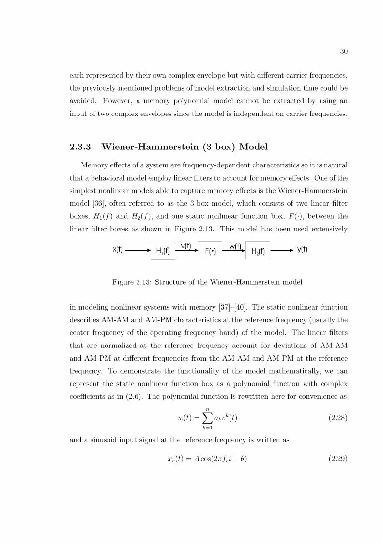
2.3.3 Wiener-Hammerstein (3 box) Model
Memory effects of a system are frequency-dependent characteristics so it is natural
that a behavioral model employ linear filters to account for memory effects. One of the
simplest nonlinear models able to capture memory effects is the Wiener-Hammerstein
model [36], often referred to as the 3-box model, which consists of two linear filter
boxes, H1(f) and H2(f), and one static nonlinear function box, F (·), between the
linear filter boxes as shown in Figure 2.13. This model has been used extensively
x(t) y(t)v(t) w(t)H (f)1 H (f)2F( )·
Figure 2.13: Structure of the Wiener-Hammerstein model
in modeling nonlinear systems with memory [37]–[40]. The static nonlinear function
describes AM-AM and AM-PM characteristics at the reference frequency (usually the
center frequency of the operating frequency band) of the model. The linear filters
that are normalized at the reference frequency account for deviations of AM-AM
and AM-PM at different frequencies from the AM-AM and AM-PM at the reference
frequency. To demonstrate the functionality of the model mathematically, we can
represent the static nonlinear function box as a polynomial function with complex
coefficients as in (2.6). The polynomial function is rewritten here for convenience as
w(t) =n∑
k=1
akvk(t) (2.28)
and a sinusoid input signal at the reference frequency is written as
xr(t) = A cos(2πfrt + θ) (2.29)
31
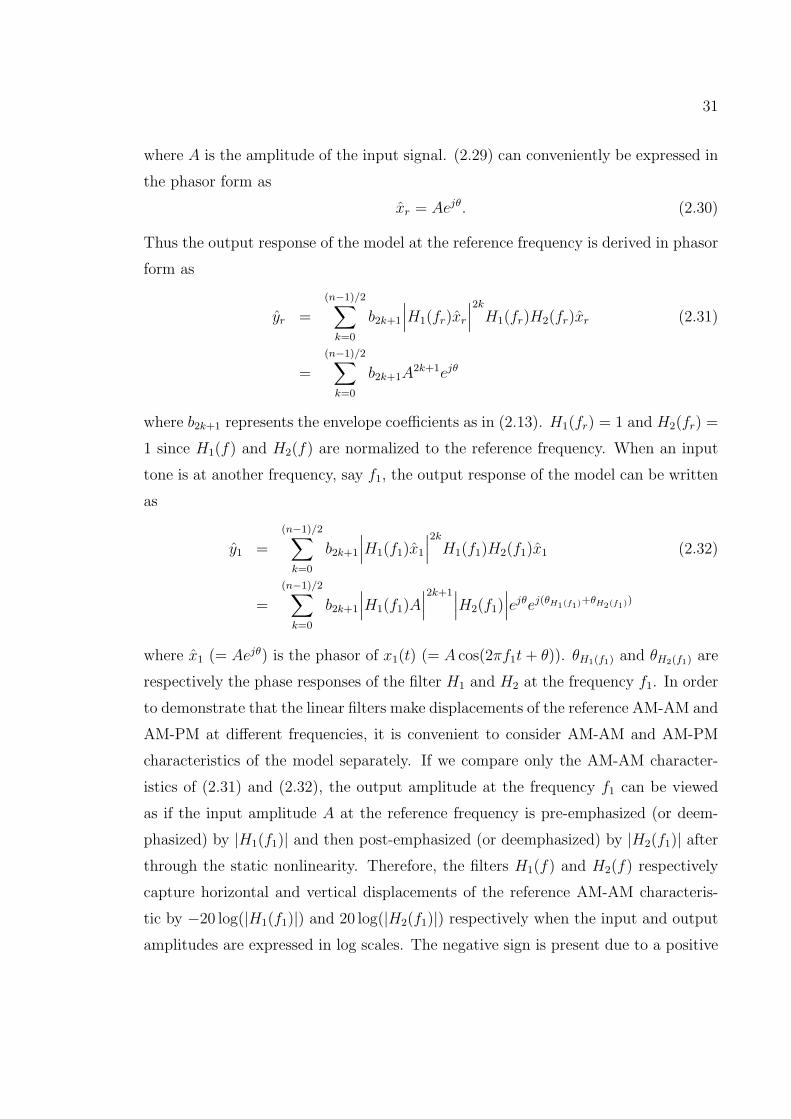
where A is the amplitude of the input signal. (2.29) can conveniently be expressed in
the phasor form as
xr = Aejθ. (2.30)
Thus the output response of the model at the reference frequency is derived in phasor
form as
yr =
(n−1)/2∑
k=0
b2k+1
∣∣∣H1(fr)xr
∣∣∣2k
H1(fr)H2(fr)xr (2.31)
=
(n−1)/2∑
k=0
b2k+1A2k+1ejθ
where b2k+1 represents the envelope coefficients as in (2.13). H1(fr) = 1 and H2(fr) =
1 since H1(f) and H2(f) are normalized to the reference frequency. When an input
tone is at another frequency, say f1, the output response of the model can be written
as
y1 =
(n−1)/2∑
k=0
b2k+1
∣∣∣H1(f1)x1
∣∣∣2k
H1(f1)H2(f1)x1 (2.32)
=
(n−1)/2∑
k=0
b2k+1
∣∣∣H1(f1)A∣∣∣2k+1∣∣∣H2(f1)
∣∣∣ejθej(θH1(f1)+θH2(f1))
where x1 (= Aejθ) is the phasor of x1(t) (= A cos(2πf1t + θ)). θH1(f1) and θH2(f1) are
respectively the phase responses of the filter H1 and H2 at the frequency f1. In order
to demonstrate that the linear filters make displacements of the reference AM-AM and
AM-PM at different frequencies, it is convenient to consider AM-AM and AM-PM
characteristics of the model separately. If we compare only the AM-AM character-
istics of (2.31) and (2.32), the output amplitude at the frequency f1 can be viewed
as if the input amplitude A at the reference frequency is pre-emphasized (or deem-
phasized) by |H1(f1)| and then post-emphasized (or deemphasized) by |H2(f1)| after
through the static nonlinearity. Therefore, the filters H1(f) and H2(f) respectively
capture horizontal and vertical displacements of the reference AM-AM characteris-
tic by −20 log(|H1(f1)|) and 20 log(|H2(f1)|) respectively when the input and output
amplitudes are expressed in log scales. The negative sign is present due to a positive
32
(or negative) horizontal shift when |H1(f1)| < 1 (or |H1(f1)| > 1). If we look at the
AM-PM characteristics of (2.31) and (2.32) and find that |H2(f1)| makes no contri-
bution to the output phase modulation, then the output phase at the frequency f1
can be written as
∠y1 = Φ(|H1(f1)|A) + θH1(f1) + θH2(f1) (2.33)
where Φ(·) is defined as
∠yr = ∠( (n−1)/2∑
k=0
b2k+1A2k+1
)+ θ (2.34)
= Φ(A) .
From (2.33) and (2.34), the AM-PM response at the frequency f1 looks as if the AM-
PM response at the reference frequency is horizontally shifted by −20 log(|H1(f1)|)and then is vertically shifted by θH1(f1) + θH2(f1) as shown in Figure 2.14. The dashed
fref
f1
Input power (dBm)
Outp
utp
ha
se(d
eg
ree
)
èH (f )2 1H (f )1 1
è +
|20log(|H (f )|)|1 1
Figure 2.14: AM-PM responses of the Wiener-Hammerstein model
line in Figure 2.14 represents a horizontal displacement of the reference AM-PM
response and the two solid lines are assumed to be measured AM-PM responses at
the reference frequency, fref , and the frequency f1 each.
33
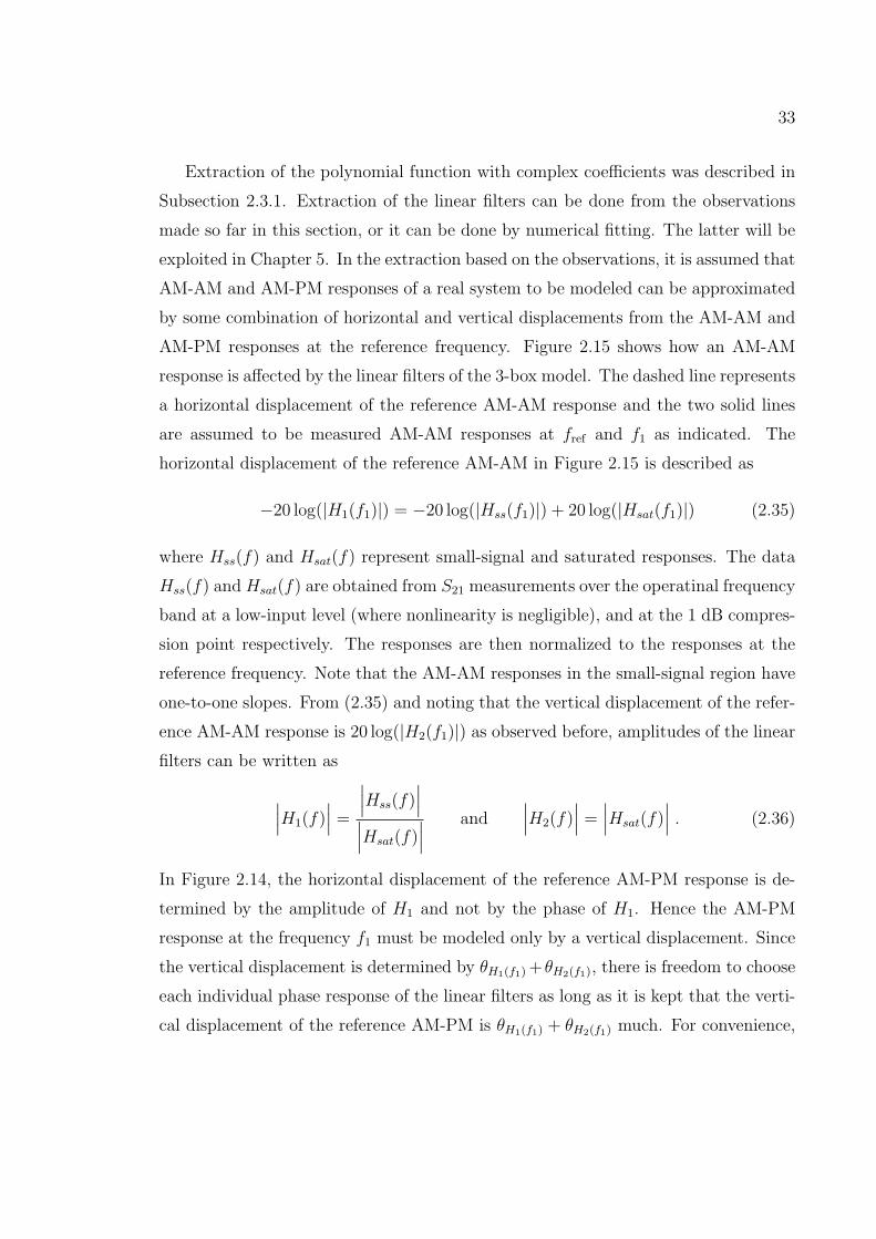
Extraction of the polynomial function with complex coefficients was described in
Subsection 2.3.1. Extraction of the linear filters can be done from the observations
made so far in this section, or it can be done by numerical fitting. The latter will be
exploited in Chapter 5. In the extraction based on the observations, it is assumed that
AM-AM and AM-PM responses of a real system to be modeled can be approximated
by some combination of horizontal and vertical displacements from the AM-AM and
AM-PM responses at the reference frequency. Figure 2.15 shows how an AM-AM
response is affected by the linear filters of the 3-box model. The dashed line represents
a horizontal displacement of the reference AM-AM response and the two solid lines
are assumed to be measured AM-AM responses at fref and f1 as indicated. The
horizontal displacement of the reference AM-AM in Figure 2.15 is described as
where Hss(f) and Hsat(f) represent small-signal and saturated responses. The data
Hss(f) and Hsat(f) are obtained from S21 measurements over the operatinal frequency
band at a low-input level (where nonlinearity is negligible), and at the 1 dB compres-
sion point respectively. The responses are then normalized to the responses at the
reference frequency. Note that the AM-AM responses in the small-signal region have
one-to-one slopes. From (2.35) and noting that the vertical displacement of the refer-
ence AM-AM response is 20 log(|H2(f1)|) as observed before, amplitudes of the linear
filters can be written as
∣∣∣H1(f)∣∣∣ =
∣∣∣Hss(f)∣∣∣
∣∣∣Hsat(f)∣∣∣
and∣∣∣H2(f)
∣∣∣ =∣∣∣Hsat(f)
∣∣∣ . (2.36)
In Figure 2.14, the horizontal displacement of the reference AM-PM response is de-
termined by the amplitude of H1 and not by the phase of H1. Hence the AM-PM
response at the frequency f1 must be modeled only by a vertical displacement. Since
the vertical displacement is determined by θH1(f1) +θH2(f1), there is freedom to choose
each individual phase response of the linear filters as long as it is kept that the verti-
cal displacement of the reference AM-PM is θH1(f1) + θH2(f1) much. For convenience,
34
20log(|H (f )|)sat 1
fref
f1
|20log(|H (f )|)|ss 1
20log(|H (f )|)sat 1
|20log(|H (f )|)|1 1
Input power (dBm)
Outp
utp
ow
er (d
Bm
)
11
Figure 2.15: AM-AM responses of the Wiener-Hammerstein model
choose the phase response of H1 as
∠H1(f) = ∠Hss(f) (2.37)
and then the phase response of H2 becomes
∠H2(f) = φ− ∠Hss(f) (2.38)
where φ is defined as θH1(f) + θH2(f). Therefore, from (2.36), (2.37) and (2.38), the
frequency response of the linear filters can be derived as
H1(f) =Hss(f)∣∣∣Hsat(f)
∣∣∣and H2(f) =
∣∣∣Hsat(f)∣∣∣ej(φ−∠Hss(f)) . (2.39)
Even though a real RF system does not exactly exhibit horizontally and vertically
displaced responses of the reference AM-AM and AM-PM responses at frequencies
other than the reference frequency, (2.39) has been formed to be a fairly good ap-
proximation up to a 1 dB compression point.
Advantages of the Wiener-Hammerstein model are simplicities in terms of model
structure and extraction. In addition it can capture memory effects; however, it can
35
only capture short-term memory effects since the linear filters of the model only char-
acterize the passband of a system. In particular, the linear filters are usually extracted
from single-tone measurements. The tone is swept in frequency and amplitude over a
passband so, at the first place, the measured data cannot include long-term memory
effects as these cannot be observed. Putting this in another context, long-term mem-
ory effects cannot be captured even with perfect model extraction from the measured
data. Even if a more realistic test signal was used, such as a digitally-modulated
signal, the presence of long-term memory effects in the measured data would result in
large model extraction error if the extraction were possible. Therefore, this is a struc-
tural problem of the model. However, the model captures short-term memory over
a wide frequency band fairly well so it is utilized as part of a multi-slice behavioral
model for multichannel applications in Chapter 4.
2.4 Simulating RF models
2.4.1 Transient Analysis
An electronic circuit consists of linear and nonlinear elements. Linear elements
include resistors, capacitors and inductors. Nonlinear elements include diodes, tran-
sistors etc. In a transient analysis linear elements are expressed in corresponding lin-
ear constitutive relations and nonlinear elements are modeled by nonlinear dependent
sources. Thus a circuit can be expressed in nonlinear algebraic equations developed
using KCL and KVL in the time domain. In transient analysis the equations are
solved at each sampling time by Newton iterations. The solutions are instantaneous
node voltages and branch currents. In transient analysis the derivatives utilized in
Newton iteration are changes of voltages or currents (or state variables) with respect
to time so computation of derivatives is based on voltages and currents at the prior
time step.
One of the advantages of transient analysis is that it can handle virtually all
types of signals including discrete tones, digital signals, noise and digitally-modulated
36
signals. However there are limitations in handling modulated RF signals such as AM,
FM, digitally-modulated signals where the information signal changes very slowly
compared to the modulated signal. To obtain reliable results in transient analysis
requires tremendous computational demands as simulation must proceed for a long
time. This results in accumulated numerical error as well as the simulation times being
unreasonably long. Therefore transient analysis is not suitable for the simulation of
RF front ends handling modulated signals.
2.4.2 Harmonic Balance Analysis
In harmonic balance analysis a circuit is partitioned into linear and nonlinear
sub-circuits as shown in Figure 2.16. The linear sub-circuit includes linear elements
Nonlinear
sub-circuit
Linear
sub-circuit
iNL iL
vNL
+
_vL
+
_
Figure 2.16: Partition of a circuit in harmonic balance
and independent sources. The rest of the circuit is included in the nonlinear sub-
circuit. The linear and the nonlinear sub-circuit are respectively computed in the time
and frequency domains. Simulation progress by equating the voltages and currents
at the interface of the two sub-circuits. For example, the linear currents iL are
initially estimated and then the linear voltages vL are computed. This evaluation is
performed in the frequency domain, that is, iL and vL are expressed as phasors. Next
the phasors of the linear voltage are converted to time-domain signals by an inverse
Fourier transform and are equated to the nonlinear voltages vNL. Next the nonlinear
currents iNL are computed from the nonlinear voltage. Finally the nonlinear current
is converted to phasors using a Fourier transform and compared to the linear current
phasors. If the differences of the linear and the nonlinear voltage phasors are above
37
a preassigned tolerance, the linear voltage phasors are updated to values that reduce
the differences. This process is performed iteratively until the differences are below
the tolerance and ‘balanced’ currents are obtained for the two sub-circuits.
Harmonic balance analysis is not affected by the frequency of the drive signal;
however, it can handle only a drive signal that can be expressed as a sum of time-
independent discrete tones in the frequency domain. Since there is no derivative in
a linear sub-circuit equations, solutions are always time-independent phasors. Thus
harmonic balance captures only steady-state responses and it cannot handle mod-
ulated RF signals that cannot be expressed as a combination of time-independent
discrete tones.
2.4.3 Conventional Envelope Transient Analysis
Digitally-modulated signals cannot be represented as discrete tones nor conve-
niently as time-domain waveforms. A single digitally-modulated channel appears as
an RF tone whose amplitude and phase vary relatively and extremely slowly cor-
responding to the amplitude and phase variations constituting the envelope of the
signal. For example, a modulation signal in the WCDMA format is 5 MHz wide with
a carrier frequency around 2 GHz. Thus the modulation signal appears to vary by one
cycle in amplitude and phase over 400 or so RF cycles. The Envelope Transient (ET)
method can be used efficiently with modulated signals as the signal is modeled as
a sequence of time-varying phasors. The variation of these phasors constitutes the
envelope of the signal. Thus analysis can progress as a large sequence of single-tone
Harmonic Balance (HB) simulations with low frequency (envelope) derivatives link-
ing the simulations. Representing a digitally-modulated signal as a slowly-varying
phasor, transforms a circuit simulation problem into a two-rate problem [41] with a
fast rate for the RF carrier and a slow rate being used to capture the modulation
envelope and baseband effects. More specifically low-frequency derivatives capture
long-term memory effects when a suitable model is used that inherently models these
effects.
As in the conventional HB technique, a circuit is partitioned into linear and non-
38
linear subcircuits with state variables of the nonlinear elements effectively interfacing
the subcircuits. The circuit equations describing the two subcircuits are written in
the frequency domain as
X(ω) = A(ω)Y (ω) + B(ω)G(ω) −∞ < ω < ∞ (2.40)
and in the time domain as
y(t) = f(x(t)). (2.41)
Here X(ω), Y (ω) and G(ω) are spectra of the state variables, x(t), the electrical vari-
ables, y(t), and the driving sources, g(t), respectively. Also, A(ω) and B(ω) are the
transfer functions characterizing the linear subcircuits. Note that the use of arbitrary
state variables does not restrict the linear circuit to having just admittance descrip-
tions. The nonlinear subcircuit is described by instantaneous relations between the
individual state variables of x and the components of y. With a digitally-modulated
excitation the carrier signal and its harmonics have time-varying envelopes having
the form
z(t) = <[ N∑
k=0
Zk(t)ejkω0t
](2.42)
=1
2
N∑
k=0
(Zk(t)e
jkω0t + Z∗k(t)e−jkω0t
)
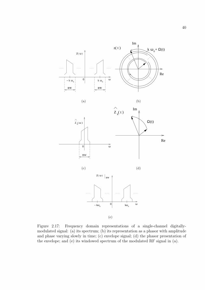
where Zk(t) is the time varying complex envelope of the k th harmonic. Figure 2.17
present the relationship between z(t) and Zk(t) in the 2-dimensional vector domain.
Figure 2.17(a) is the spectrum of the k th harmonic of the digitally-modulated sig-
nal z(t) showing both the positive and the negative frequency-domain components.
A representation of the digitally-modulated signal as an RF phasor is given in Fig-
ure 2.17(b) where the amplitude and the phase of the phasor vary with time. The
spectrum of the envelope portion of the modulated signal, i.e. Zk(t), is shown in Fig-
ure 2.17(c) and its phasor representation in Figure 2.17(d). The projections of the z(t)
and Zk(t) vectors on the real axis are the original signal and envelope, respectively,
in the time domain.
39
The first key concept of the ET method is the use of two time scales. This
enables the computation of a time-varying envelope on a slow time scale while the
high frequency effects are on a fast time scale. Rewriting (2.42) with two time scales
yields:
z(t1, t2) = <[ N∑
k=0
Zk(t1)ejkω0t2
](2.43)
=1
2
N∑
k=0
(Zk(t1)e
jkω0t2 + Z∗k(t1)e
−jkω0t2)
where ω0 is the RF carrier frequency. The time scale t1 is used with the complex
envelopes and t2 is used with the high frequency signals including the carrier and its
harmonics. The second key concept is transforming that part of the problem with
the fast time scale into a problem that can be solved in the frequency domain. Thus
we define Zk(t1), the inverse Fourier transform of Zk(ω) as
Zk(t1) =1
2π
∫ BW/2
−BW/2
Zk(ω)ejωt1dω (2.44)
where BW is the bandwidth of the spectrum of the RF signal as shown in Fig-
ure 2.17(c). BW is inversely proportional to the size of the time step when Zk(t) is
discretized with respect to time. Similarly Zk(ω) is the spectral component of z(t)
centered at the k th harmonic of the RF carrier. Zk(ω) can be thought of as the
positive frequency spectrum of Zk(ω) windowed around kω0 and down-converted by
kω0. The amplitude of Zk(ω) is two times that of Zk(ω). From (2.43) and (2.44) it
can be seen that the Fourier transform of z(t) can be approximated without loss of
signal information as
Z(ω)∣∣∣BW
=1
2
N∑
k=0
(Zk(ω − kω0) + Z∗
k(−ω − kω0))
(2.45)
where Z(ω)|BW represents spectrums within the bandwidth BW around each of the
harmonics of the RF carrier, i.e. ±kω0 as in Figure 2.17(e). Thus with either Zk(ω)
or with Zk(t1) the total truncated spectrum Z(ω)|BW can be obtained.
Now x(t), y(t) and g(t) of (2.40) are in the same form as z(t) so that the spectra
of envelopes of x(t), y(t) and g(t) at kω0 are conveniently represented as Xk(ω−kω0),
40
BW
ω0
k
BW
ω0
− k 0
Z( )ω
ω
(a)
(t)+ Ωω0
Im
Re
z( t ) k
(b)
ωZ ( )k
BW
0 ω
(c)
(t)Ω
Z ( t )k
Im
Re
(d)
ω0
k− ω0
k
Z( )ωBW
0 ω
(e)
Figure 2.17: Frequency domain representations of a single-channel digitally-modulated signal: (a) its spectrum; (b) its representation as a phasor with amplitudeand phase varying slowly in time; (c) envelope signal; (d) the phasor presentation ofthe envelope; and (e) its windowed spectrum of the modulated RF signal in (a).
41
Yk(ω−kω0) and Gk(ω−kω0) respectively. Then the linear subcircuit equation, (2.40),
with Ω = ω − kω0. In effect, the RF signals are frequency down-converted enabling
ω0
k
ω0
k
ω
kωY ( − )
(a)
ω0
k
A( )ω
ω
(b)
Y ( )Ωk
Ω0
(c)
ω0
kΩA( + )
Ω0
(d)
Figure 2.18: (a) spectrum of the electrical variable; (b) its transfer function; (c)down-converted spectrum and (d) down-converted transfer function.
high frequency components to be obtained by computing the circuit equations on the
slow time scale as shown in Figure 2.18. The linear transfer function A(Ω + kω0) in
(2.47) can be expanded in a Taylor series:
A(Ω + kω0) = A(ω)|ω=kω0 + ΩdA(ω)
dω
∣∣∣ω=kω0
(2.48)
+Ω2
2
d2A(ω)
dω2
∣∣∣ω=kω0
+ · · ·
42
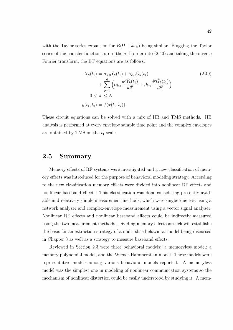
with the Taylor series expansion for B(Ω + kω0) being similar. Plugging the Taylor
series of the transfer functions up to the q th order into (2.40) and taking the inverse
Fourier transform, the ET equations are as follows:
Xk(t1) = αk,0Yk(t1) + βk,0Gk(t1) (2.49)
+
q∑p=1
(αk,p
dpYk(t1)
dtp1+ βk,p
dpGk(t1)
dtp1
)
0 ≤ k ≤ N
y(t1, t2) = f(x(t1, t2)).
These circuit equations can be solved with a mix of HB and TMS methods. HB
analysis is performed at every envelope sample time point and the complex envelopes
are obtained by TMS on the t1 scale.
2.5 Summary
Memory effects of RF systems were investigated and a new classification of mem-
ory effects was introduced for the purpose of behavioral modeling strategy. According
to the new classification memory effects were divided into nonlinear RF effects and
nonlinear baseband effects. This classification was done considering presently avail-
able and relatively simple measurement methods, which were single-tone test using a
network analyzer and complex-envelope measurement using a vector signal analyzer.
Nonlinear RF effects and nonlinear baseband effects could be indirectly measured
using the two measurement methods. Dividing memory effects as such will establishe
the basis for an extraction strategy of a multi-slice behavioral model being discussed
in Chapter 3 as well as a strategy to measure baseband effects.
Reviewed in Section 2.3 were three behavioral models: a memoryless model; a
memory polynomial model; and the Wiener-Hammerstein model. These models were
representative models among various behavioral models reported. A memoryless
model was the simplest one in modeling of nonlinear communication systems so the
mechanism of nonlinear distortion could be easily understood by studying it. A mem-
43
ory polynomial model was one of the rare models that could capture baseband effects.
However it could not capture baseband effects systemically and rigorously. Thus the
performance of the model was questionable. The Wiener-Hammerstein model was
known to capture memory effects but it could only capture short-term memory ef-
fects. Reviewing these behavioral models will help to understand the structure of
a multi-slice behavioral model and the mechanism to systemically capture memory
effects with it. The Wiener-Hammerstein model will be utilized later in multi-slice
behavioral modeling.
Reviewed in Section 2.4 were three circuit simulation techniques: transient; har-
monic balance; and envelope transient. Transient and harmonic balance were briefly
reviewed since these techniques were utilized in envelope transient. Envelope transient
was thoroughly reviewed since it could simulate RF circuits excited with digitally-
modulated signals and capture baseband effects. Thus it could be used in capturing
baseband effects of multichannel communication systems. The mechanism of captur-
ing baseband effects was not clear in the conventional envelope transient so it will
be clarified in Chapter 4. Also, the conventional envelope transient will be extended
to multichannel envelope transient that can handle multichannel digitally modulated
signals. A multi-slice behavioral model will be used in multichannel envelope transient
simulation and transient simulation in Chapter 5.
44
Chapter 3
Multi-Slice Behavioral Model
3.1 Introduction
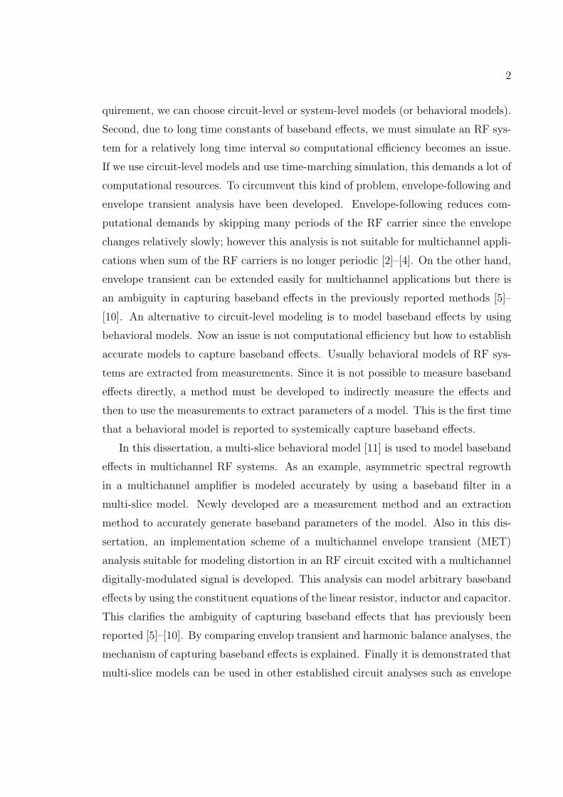
As a preliminary step toward capturing baseband effects (or electrical long-term
memory effects) in multichannel communication systems, a multi-slice behavioral
model is developed that captures baseband memory effects of a single-channel power
amplifier. This work is described by the author in [48]. The model consists of two
slices and systemically captures baseband effects of an RF system. The first slice of
the model is a static nonlinear function (an odd-order polynomial having complex
coefficient), which captures memoryless nonlinearities of an RF system. The second
slice consists of a static nonlinear function (an even-order polynomial), a frequency-
domain baseband filter and an ideal mixer. The static nonlinear function is used to
produce baseband products and the frequency-domain baseband filter is used to shape
the baseband products. And then the output of the baseband filter is up-converted to
the fundamental frequency band by a mixer to account for baseband effects. The first
and the second slice of the model are respectively extracted using measurements with
a single tone and a single-channel WCDMA signal. The measurements are in the form
of complex envelope so they are easy to obtain using a vector signal analyzer. The
45
parameters of the model are extracted by directly comparing with the measurements.
In Section 3.2, the specific model architecture is described and how the model
captures baseband effects is discussed. In Section 3.3, a procedure for experimentally
characterizing a system and extracting the model is presented. In Section 3.4, a
commercial power amplifier and a WCDMA signal are used to extract the multi-slice
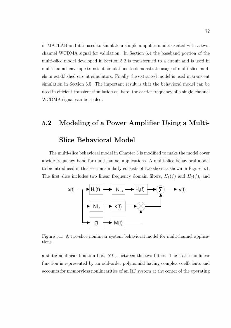
model. The work is validated by comparing measured and modeled results.
3.2 Model Architecture
For single-channel applications, a multi-slice behavioral model was developed to
capture baseband memory effects that are important in capturing the nonlinear be-
havior of power amplifiers. Two slices are used for simplicity although the multi-slice
model, Figure 3.1, can be extended to cover additional operational behavior. Any
NL1
NL2 H(f)
Óx(t) y(t)
Figure 3.1: A two-slice nonlinear system behavioral model.
form of a behavioral model can be used in each slice. In this work and referring to
Figure 3.1, the first slice is represented by an odd-order polynomial having complex
coefficients and capturing memoryless contributions to the fundamental response.
The second slice consists of a static nonlinear function, a linear frequency domain
filter, H(f), and an ideal mixer. The static nonlinear function is represented by an
even-order polynomial with complex coefficients. In effect the nonlinearity in the
second slice generates baseband frequency components. The linear filter in the sec-
ond slice appropriately shapes the spectrum of baseband produced by the even-order
46
nonlinearity and the ideal mixer up-converts the output of H(f) to the fundamental.
Hence, the second slice accounts for baseband memory effects that cause asymmetric
spectral regrowth.
3.3 Extraction Procedure
The measurement and extraction procedure for the odd-order polynomial coeffi-
cients in the first slice is the same as that described in Subsection 2.3.1. Thus the
first slice captures the AM-AM and AM-PM characteristics of a system. To obtain
an accurate memoryless model, it is important to extract low-order coefficients as
accurately as possible. This is particularly true for first-order and third-order coef-
ficients, which are generally extracted from measured S21 when input amplitude is
low. Since the dynamic range of a network analyzer is limited, the measured S21 data
tends to be unreliable. Impression is particularly evident for the phase response as
it includes a lot of noise when the signal levels are low. It was found that the effect
of noise can be removed by averaging multiple measurement. Measurements required
for extraction of the second slice were collected using a vector signal analyzer. In
this case the input is a single-channel digitally-modulated signal whose bandwidth is
equal to the bandwidth of the baseband circuit. When the power of the input is low
enough that the third-order nonlinearity is dominant, the output complex envelope
at the fundamental is measured to extract the coefficient of x2(t) and H(f). This
measured output includes distortions caused by memoryless nonlinearities and long-
term memory effects if it is assumed that short-term memory effects are negligibly
small due to the bandwidth of the single-channel input. If we remove the distor-
tions caused by the memoryless nonlinearities from the measured output, then the
result will only have the distortions caused by the long-term memory effects. Hence,
the post-processed result is treated as the measured output for the extraction. As
shown in Figure 3.2, the response required in extraction is obtained by subtracting
the modeled output of the first slice from the measured response to the digitally-
modulated input. Thus baseband effects in the post-processed data are caused by
47
NL1
NL2 H(f)
Ó
x(t)
e(t)Ó
+
_
_
+
power amplifier
Figure 3.2: A block diagram showing extraction procedure of the two-slice nonlinearsystem behavioral model.
the second-order nonlinearity so the first block of the second slice is set to x2(t) and
H(f) becomes the only unknown block left to be extracted. H(f) is just a transfer
function relating the input and output of H(f) and is obtained by direct computa-
tion. Conversion between the time domain and the frequency domain is done by the
Fourier transform. Following extraction of H(f), it is normalized and the coefficient
of x2(t) is adjusted accordingly. Strictly speaking, the complex coefficient extracted
for the even-order polynomial nonlinear model of the second slice models a complex
gain block and simplifies the model structure. Higher-order nonlinear baseband ef-
fects are modeled from data obtained by sweeping amplitude of the input signal and
measuring the output response using the extraction procedure described above. Now
however, since H(f) is already determined, higher-order coefficients of the even-order
polynomial are extracted.
3.4 Verification
A gallium arsenide (GaAs) hetero-junction bipolar transistor (HBT) power am-
plifier (RF Micro Devices model RF5117) designed for wireless local area network
(WLAN) applications was used to extract parameters of the multi-slice model. Gain
48
of the amplifier was around 25 dB at 2.5 GHz. The nonlinear block in the first slice
was extracted from the single-tone AM-AM and AM-PM characteristics at the carrier
frequency (2.5 GHz) and fitted to a 17 th-order odd-order complex polynomial. The
measured and modelled characteristics are almost identical as seen in Figures 3.3 and
3.4. Initially two-tone testing was used to extract the model of the second slice. It
0 0.05 0.1 0.15 0.2 0.25 0.3 0.350
1
2
3
4
5
6
Input (V)
Out
put (
V)
dash: measureddot: modeled
Figure 3.3: Measured and modelled AM-AM characteristics of the amplifier at2.5 GHz. (The measured and modelled characteristics overlap.)
was found that a precise model could not be easily obtained even if the frequency
separation of the two tones was swept. This is attributed to accumulated errors in
the difference technique used in extracting the second-slice data. However a reli-
able model could be extracted using a digitally-modulated signal. The second slice
was successfully extracted by comparing the response to a digitally-modulated input
signal to that calculated by the first-slice alone. In particular, a Wideband Code
Division Multiple Access (WCDMA) down-link signal was used and the response is
measured by a Vector Signal Analyzer (VSA: Agilent Model 89600S). An input power
level of −11 dBm was chosen for initial extraction of the second slice model as at this
power level nonlinear response is significant. The difference between the measured
49
0.1 0.15 0.2 0.25 0.3 0.35−175
−174
−173
−172
−171
−170
−169
−168
−167
−166
−165
Input (V)
Out
put (
degr
ee)
dash: measureddot: modeled
Figure 3.4: Measured and modelled AM-PM characteristics of the amplifier at2.5 GHz. (The measured and modelled characteristics overlap.)
response and that modelled by the first slice leads to the baseband transfer function
response, H(f), shown in Figures 3.5 and 3.6. The baseband nonlinear behavior, cap-
tured by NL2, was obtained from the measurements of the response to the WCDMA
signal swept in amplitude and fitted to an even-order complex polynomial. Note
the approximate odd symmetry in the phase response of H(f) in Figure 3.6. This
leads to an approximate conjugate relationship between lower-side and upper-side
intermodulation products resulting from baseband effects. Note that the extracted
H(f) transfer function (Figures 3.5 and 3.6) are not fully physical since the transfer
characteristics of the amplitude and phase fluctuations are not realistic and they are
not precisely conjugate. This is a result of the extraction being based on measure-
ments of the response to a digitally-modulated signal. However this model faithfully
models behavior over a range of power levels. H(f) can be extracted in other ways
using, for example, the two-tone equivalent of AM-AM and AM-PM characterizations
over a range of tone separations. In Section 5.2, another extraction method will be
introduced to produce a realistic H(f) using two-tone IM3 amplitude measurements
as well as complex-envelope measurements. Modelled results are compared with mea-
50
−4 −3 −2 −1 0 1 2 3 40
0.1
0.2
0.3
0.4
0.5
0.6
0.7
0.8
0.9
1
Frequency (MHz)
Mag
nitu
de n
orm
aliz
ed
Figure 3.5: Normalized magnitude of H(f) which is used directly in the model.
−4 −3 −2 −1 0 1 2 3 4−200
−150
−100
−50
0
50
100
150
200
Frequency (MHz)
Pha
se (
degr
ee)
Figure 3.6: Modelled phase characteristics of H(f) which is used directly in the model.
51
surements in Figure 3.7. They agree very well where input power is swept from −11
−10 −5 0 5 10−90
−80
−70
−60
−50
−40
−30
−20
−10
0
Offset Frequency (MHz) @ 2.5GHz
Out
put A
mpl
itude
(dB
m)
Measured: solid lineModeled: dashed line
Figure 3.7: Measured and modelled output frequency spectra of the WLAN amplifier.
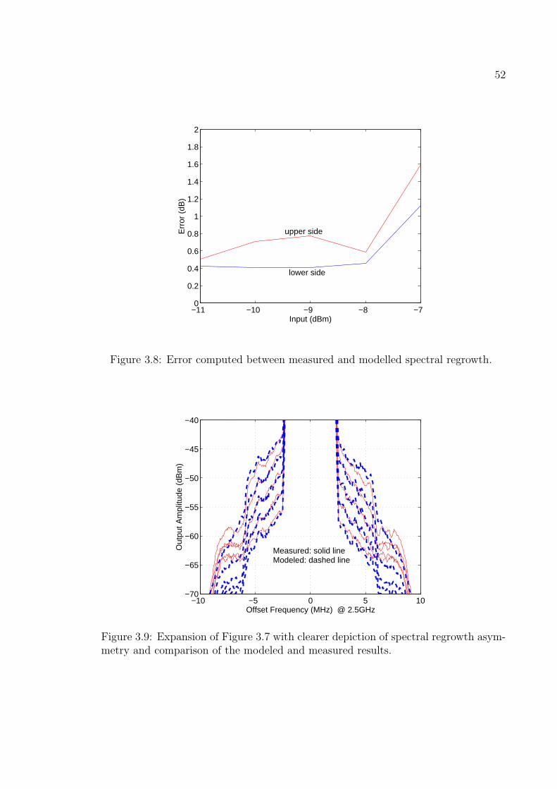
to −7 dBm. The averaged discrepancy of the spectral regrowth is computed as
E =
∑Nf=1 |P (f) meas − P (f) mod|
N(3.1)
where P (f) meas and P (f) mod are respectively measured and modeled values of power
at a discrete frequency f . The resulting error as a function of input is depicted in
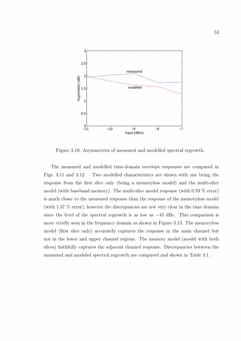
Figure 3.8. To visualize asymmetric spectral regrowth, the data in Figure 3.7 is re-
plotted on an expanded scale in Figure 3.9. About 2 dB of asymmetry is observed
in the lower and upper spectral regrowth response. The measured and modeled
asymmetries are computed and compared in Figure 3.10. Discrepancies of the noise
level at the far sides of the channel in Figure 3.9 are originated from the input signal
to the model. The input signal is measured several times and averaged to lower the
noise level. This solves the dynamic range problem of a vector signal analyzer when
an input level is low. Thus the noise level of modeled output is different from that of
the measured output that is not averaged.
52
−11 −10 −9 −8 −70
0.2
0.4
0.6
0.8
1
1.2
1.4
1.6
1.8
2
Input (dBm)
Err
or (
dB)
upper side
lower side
Figure 3.8: Error computed between measured and modelled spectral regrowth.
−10 −5 0 5 10−70
−65
−60
−55
−50
−45
−40
Offset Frequency (MHz) @ 2.5GHz
Out
put A
mpl
itude
(dB
m)
Measured: solid lineModeled: dashed line
Figure 3.9: Expansion of Figure 3.7 with clearer depiction of spectral regrowth asym-metry and comparison of the modeled and measured results.
53
−11 −10 −9 −8 −70
0.5
1
1.5
2
2.5
3
Input (dBm)
Asy
mm
etry
(dB
)
measured
modeled
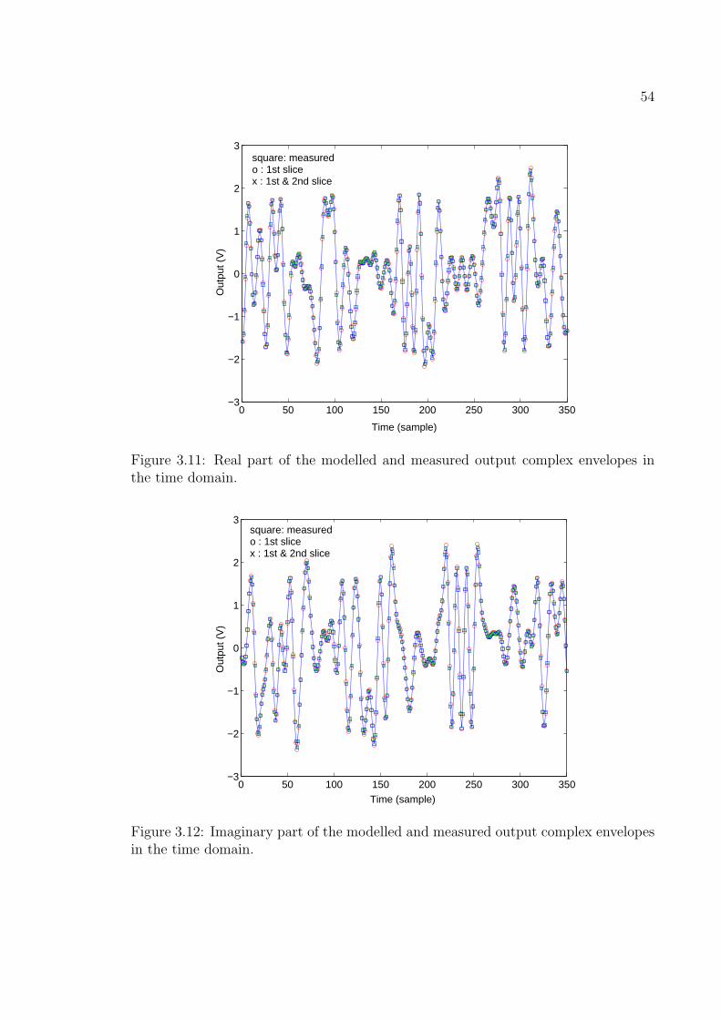
Figure 3.10: Asymmetries of measured and modelled spectral regrowth.
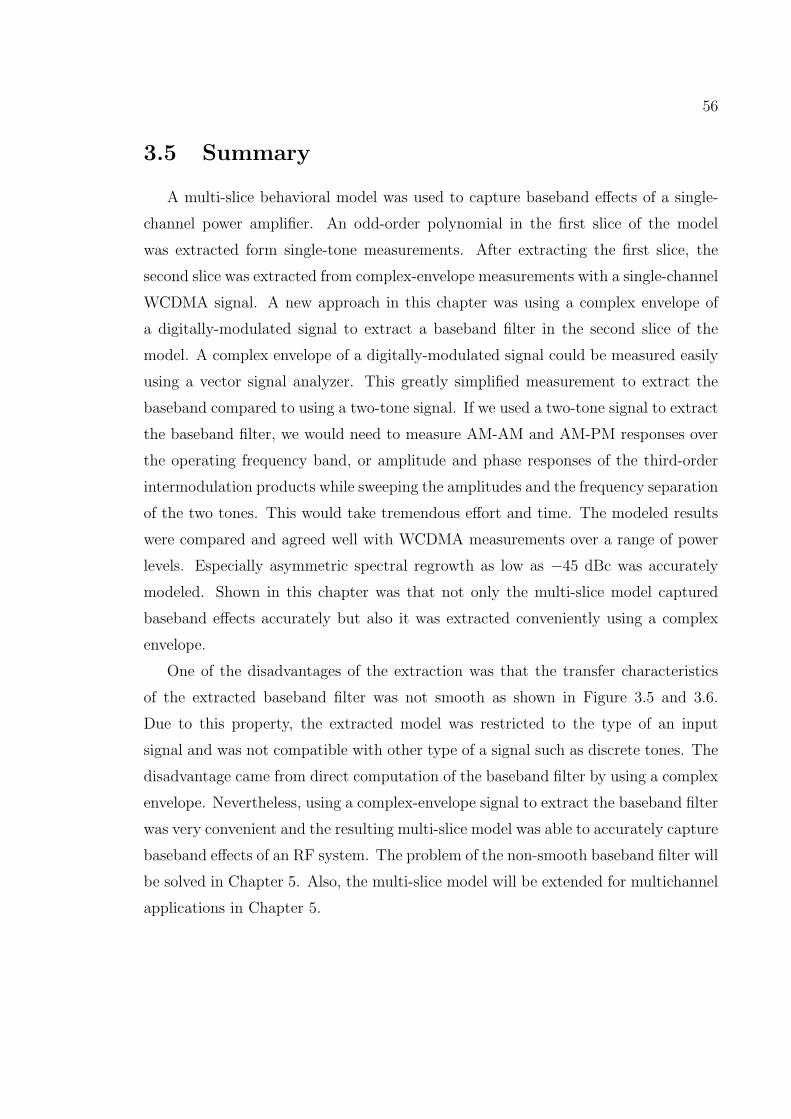
The measured and modelled time-domain envelope responses are compared in
Figs. 3.11 and 3.12. Two modelled characteristics are shown with one being the
response from the first slice only (being a memoryless model) and the multi-slice
model (with baseband memory). The multi-slice model response (with 0.59 % error)
is much closer to the measured response than the response of the memoryless model
(with 1.37 % error); however the discrepancies are not very clear in the time domain
since the level of the spectral regrowth is as low as −45 dBc. This comparison is
more vividly seen in the frequency domain as shown in Figure 3.13. The memoryless
model (first slice only) accurately captures the response in the main channel but
not in the lower and upper channel regions. The memory model (model with both
slices) faithfully captures the adjacent channel response. Discrepancies between the
measured and modeled spectral regrowth are computed and shown in Table 3.1.
54
0 50 100 150 200 250 300 350−3
−2
−1
0
1
2
3
Time (sample)
Out
put (
V)
square: measured o : 1st slice x : 1st & 2nd slice
Figure 3.11: Real part of the modelled and measured output complex envelopes inthe time domain.
0 50 100 150 200 250 300 350−3
−2
−1
0
1
2
3square: measured o : 1st slice x : 1st & 2nd slice
Out
put (
V)
Time (sample)
Figure 3.12: Imaginary part of the modelled and measured output complex envelopesin the time domain.
55
−10 −5 0 5 10−90
−80
−70
−60
−50
−40
−30
−20
−10
0
Offset Frequency (MHz) @ 2.5GHz
Out
put A
mpl
itude
(dB
m)
1st slice onlyMeasured
1st & 2nd slices (dashed line)
Figure 3.13: Output frequency spectra of the model with and without memory, andmeasurements.
Table 3.1: Discrepancies (in dB) between the measured and modeled spectralregrowth.
memory model memoryless modellower channel 0.42 4.14upper channel 0.50 6.03
56
3.5 Summary
A multi-slice behavioral model was used to capture baseband effects of a single-
channel power amplifier. An odd-order polynomial in the first slice of the model
was extracted form single-tone measurements. After extracting the first slice, the
second slice was extracted from complex-envelope measurements with a single-channel
WCDMA signal. A new approach in this chapter was using a complex envelope of
a digitally-modulated signal to extract a baseband filter in the second slice of the
model. A complex envelope of a digitally-modulated signal could be measured easily
using a vector signal analyzer. This greatly simplified measurement to extract the
baseband compared to using a two-tone signal. If we used a two-tone signal to extract
the baseband filter, we would need to measure AM-AM and AM-PM responses over
the operating frequency band, or amplitude and phase responses of the third-order
intermodulation products while sweeping the amplitudes and the frequency separation
of the two tones. This would take tremendous effort and time. The modeled results
were compared and agreed well with WCDMA measurements over a range of power
levels. Especially asymmetric spectral regrowth as low as −45 dBc was accurately
modeled. Shown in this chapter was that not only the multi-slice model captured
baseband effects accurately but also it was extracted conveniently using a complex
envelope.
One of the disadvantages of the extraction was that the transfer characteristics
of the extracted baseband filter was not smooth as shown in Figure 3.5 and 3.6.
Due to this property, the extracted model was restricted to the type of an input
signal and was not compatible with other type of a signal such as discrete tones. The
disadvantage came from direct computation of the baseband filter by using a complex
envelope. Nevertheless, using a complex-envelope signal to extract the baseband filter
was very convenient and the resulting multi-slice model was able to accurately capture
baseband effects of an RF system. The problem of the non-smooth baseband filter will
be solved in Chapter 5. Also, the multi-slice model will be extended for multichannel
applications in Chapter 5.
57
Chapter 4
Multichannel Envelope Transient
Analysis
4.1 Introduction
An Envelope Transient analysis for multichannel applications [42]–[43] was theo-
retically formulated in Section 4.1. Various applications of the analysis can be found
in [44]–[47]. In the analysis, each individual channel is treated separately to achieve
better computational efficiency. In Section 4.2, formulation for circuit elements R, L
and C are constructed in the modified Nodal admittance matrix form to build a sim-
ulator. In the patent document [7], one of the original documents describing envelope
transient analysis, the linear circuit response is captured by its impulse response. In
this chapter the analysis is generalized to handle arbitrarily complex baseband cir-
cuitry described using circuit elements or by the multi-slice model introduced in the
previous chapter. To complete the developement an error function is formulated to
enable iterative circuit simulation. In Section 4.3, it is shown that the envelope tran-
sient method can capture memory effects, especially baseband effects. Derivatives of
58
the envelope transient equations around DC take baseband effects into account. As
a further illustration of capturing baseband effects, the envelope transient analysis
is compared to a sequence of HB analyses with time-varying phasors in Section 4.4.
The difference between the two analyses is inclusion of long time-constant derivatives
in envelope transient analysis that are not included in HB analysis. Finally a multi-
channel envelope transient analysis is compared to a single-channel envelope transient
analysis in Section 4.5. The impact on computational efficiency using multichannel
envelope transient analysis is demonstrated when channels are separated widely.
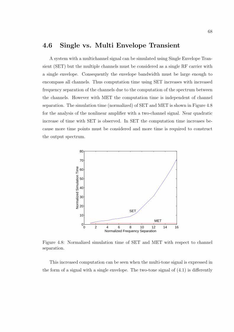
4.2 Theoretical Formulation
A two-channel digitally-modulated signal can be generally expressed in the fol-
lowing form
z(t) = Re[Z1(t)e
jω1t + Z2(t)ejω2t
](4.1)
where Z1(t) and Z2(t) represent the complex envelopes corresponding to each carrier
frequency, ω1 and ω2. This two-channel expression is used for the purpose of simplicity
but it can be simply generalized to multi-channel signals. The signal in (4.1) can
be viewed as comprising two time-varying tones. The spectrum of the signals in a
nonlinear circuit with an input g(t) (of the form of (4.1)) is shown in Figure 4.1. The
waveforms in the circuit have the general forms:
x(t) = Re[ k∑
m,n=−k
Xm,n(t)ej(mω1+nω2)t]
(4.2)
where mω1 + nω2 ≥ 0, and m and n are frequency indices. Now denote g(t) as the
two-channel source, and x(t) and y(t) as circuit waveforms. The frequency-domain
relationship of these signals is defined in (2.40). Applying the same procedures used
with Single Envelope Transient (SET), the linear circuit equation of Multi Envelope
Transient (MET) is obtained as follows:
Xm,n(t1) = αm,n,0Ym,n(t1) + βm,n,0Gm,n(t1) (4.3)
59
ω1
ω2
ts1
ts2
ts3
ts4
A φ
t
ω0
(a)
A φ
ω1
ω2
ω2
2ω1
2 ω1
3 ω2
3
ts1
ts2
ts3
ts4
ω0
t
(b)
Figure 4.1: Input and output of a nonlinear system in the complex envelope expressionview: (a) time-varying input signal; and (b) time-varying internal and output signals.
60
+
q∑p=1
(αm,n,p
dpYm,n(t1)
dtp1
+ βm,n,pdpGm,n(t1)
dtp1
)
where m and n are chosen in the manner of mω1 + nω2 ≥ 0; The source envelope,
Gm,n(t1) is non zero only at fundamental frequencies and/or DC, otherwise it is zero.
The nonlinear subcircuit is computed in the time domain as in SET.
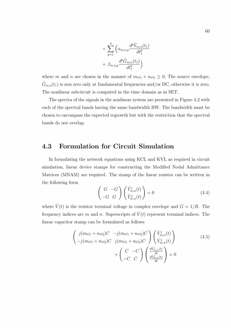
The spectra of the signals in the nonlinear system are presented in Figure 4.2 with
each of the spectral bands having the same bandwidth BW. The bandwidth must be
chosen to encompass the expected regrowth but with the restriction that the spectral
bands do not overlap.
4.3 Formulation for Circuit Simulation
In formulating the network equations using KCL and KVL as required in circuit
simulation, linear device stamps for constructing the Modified Nodal Admittance
Matrices (MNAM) are required. The stamp of the linear resistor can be written in
the following form (G −G
−G G
)(V i
m,n(t)
V jm,n(t)
)= 0 (4.4)
where V (t) is the resistor terminal voltage in complex envelope and G = 1/R. The
frequency indices are m and n. Superscripts of V (t) represent terminal indices. The
linear capacitor stamp can be formulated as follows
(j(mω1 + nω2)C −j(mω1 + nω2)C
−j(mω1 + nω2)C j(mω1 + nω2)C
)(V i
m,n(t)
V jm,n(t)
)(4.5)
+
(C −C
−C C
)
dV im,n(t)
dtdV j
m,n(t)
dt
= 0
61
0
ωBW
BW BW
1ω
2
ωω
G ( )
(a)
BW
ω
BW
02ω 2 1ω 2 2ω 3 1ω 3 2ω1ω
ωBW
X ( )
(b)
Figure 4.2: Spectrum of signals in a nonlinear system considered in MET analysis:(a) spectra of source signals; and (b) spectra of internal circuit and output signals.
62
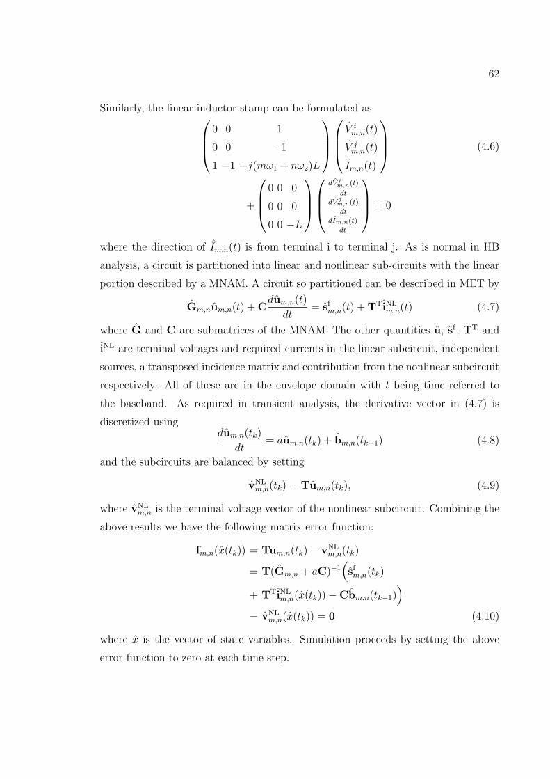
Similarly, the linear inductor stamp can be formulated as
0 0 1
0 0 −1
1 −1 −j(mω1 + nω2)L
V im,n(t)
V jm,n(t)
Im,n(t)
(4.6)
+
0 0 0
0 0 0
0 0 −L
dV im,n(t)
dtdV j
m,n(t)
dtdIm,n(t)
dt
= 0
where the direction of Im,n(t) is from terminal i to terminal j. As is normal in HB
analysis, a circuit is partitioned into linear and nonlinear sub-circuits with the linear
portion described by a MNAM. A circuit so partitioned can be described in MET by
Gm,num,n(t) + Cdum,n(t)
dt= sf
m,n(t) + TTiNLm,n(t) (4.7)
where G and C are submatrices of the MNAM. The other quantities u, sf , TT and
iNL are terminal voltages and required currents in the linear subcircuit, independent
sources, a transposed incidence matrix and contribution from the nonlinear subcircuit
respectively. All of these are in the envelope domain with t being time referred to
the baseband. As required in transient analysis, the derivative vector in (4.7) is
discretized usingdum,n(tk)
dt= aum,n(tk) + bm,n(tk−1) (4.8)
and the subcircuits are balanced by setting
vNLm,n(tk) = Tum,n(tk), (4.9)
where vNLm,n is the terminal voltage vector of the nonlinear subcircuit. Combining the
above results we have the following matrix error function:
fm,n(x(tk)) = Tum,n(tk)− vNLm,n(tk)
= T(Gm,n + aC)−1(sf
m,n(tk)
+ TTiNLm,n(x(tk))−Cbm,n(tk−1)
)
− vNLm,n(x(tk)) = 0 (4.10)
where x is the vector of state variables. Simulation proceeds by setting the above
error function to zero at each time step.
63
4.4 Baseband Effects
Baseband (low frequency or long time constant) impedance effects are captured by
the linear transfer function A(Ω+kω0) and B(Ω+kω0) in (2.47). As an example, the
component of the transfer function of a linear capacitor (with which an admittance
description is used) is represented, without approximation, as
A(Ω + kω0) = jkω0C + jΩC. (4.11)
This is just the constitutive relation of the linear capacitor in ET. The inverse Fourier
transform of (2.40) combined with (4.11) is then
Ik(t1) = jkω0CVk(t1) + CdVk(t1)
dt1(4.12)
where t1 is the time scale of the complex envelope. The derivative term in (4.12)
captures the small changes in the relationship between the capacitor current and
voltage due to the slow time-varying modulation signal. With a linear inductor an
impedance description is used and A(Ω+jkω0) = jkω0L+jΩL. Thus the constitutive
relation for a linear inductor is:
Vk(t1) = jkω0LIk(t1) + LdIk(t1)
dt1. (4.13)
Using the constitutive relations of elementary components, the fully general ET equa-
tions are as follows:
Xk(t1) = f1(Yk(t1), Gk(t1),dYk(t1)
dt1,dGk(t1)
dt1,
d2Yk(t1)
dt21,d2Gk(t1)
dt21, · · ·) (4.14)
0 ≤ k ≤ N
y(t1, t2) = f2(x(t1, t2))
where f2 is the same function as f in (2.41).
64
4.5 Harmonic Balance vs. Envelope Transient
This is a convenient point to contrast three analysis techniques: a sequence
of HB analyses with time-varying phasors; the conventional Single Envelope Tran-
sient (SET); and the enhanced Multi Envelope Transient (MET) developed here. A
digitally-modulated RF carrier, a single channel, can be viewed as a time sequence
of RF phasors. If a single-tone HB solution is performed then the only low-frequency
component will be at DC. Thus a sequence of HB solutions will only capture baseband
resistive effects. Conventional SET does capture baseband resistive and capacitive
effects through the time derivative at the slow time rate, the time derivative in (4.12).
The extended MET method here also captures baseband inductive effects provided
that a state variable based HB solver is used. ET captures the baseband signal caused
by even-order nonlinearity of the nonlinear circuit block. Accurate computation of the
baseband signal is especially important as the balancing of the I and Q chains is crit-
ical in wireless communication systems. When the amplitude of the baseband signal
is relatively large, it can affect other frequency components including fundamentals
and harmonics.
A power amplifier designed for the Personal Communications Services band with
IS-95 reverse link excitation was modelled using both time-varying HB and SET. This
amplifier, PCS pamp prj, is a part of the example set supplied with the commercial
ADS circuit simulator. The modelled performance obtained using time-varying HB
and SET are shown in Figure 4.3 with almost identical results obtained. For the time-
varying HB and SET to result in the same response, baseband impedance/admittance
is either totally resistive or very small (the baseband derivatives are zeros or close to
zeros) yet the former is unlikely to be a characteristic of the amplifier. The conclusion
is that the long-time derivatives extracted from the amplifier are negligibly small
since the only difference between time-varying HB and SET is whether there are
derivatives or not. This conclusion was verified by driving the amplifier with two tones
separated by 200 kHz with a center frequency of 1.9 GHz. The simulated magnitude
differences between lower and upper third order intermodulation (IM3) products are
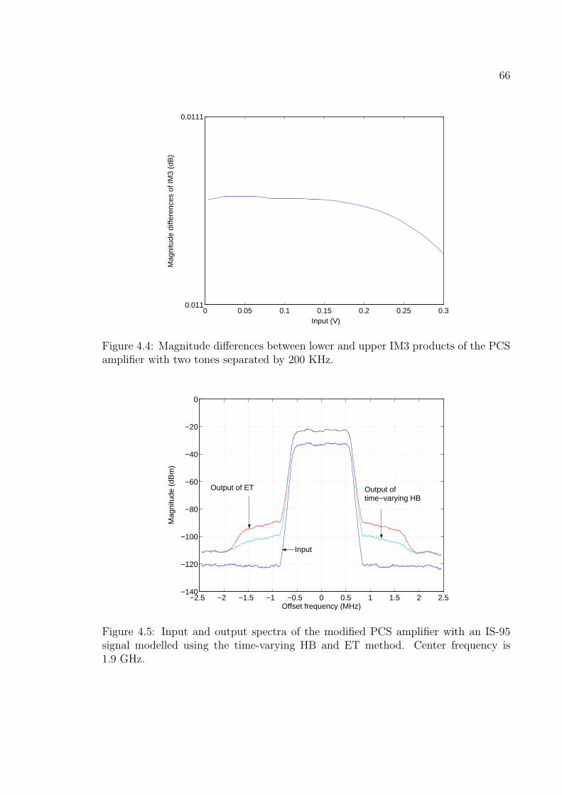
about 0.01 dB as shown in Figure 4.4, that is, there is no significant asymmetry in the
65
−2.5 −2 −1.5 −1 −0.5 0 0.5 1 1.5 2 2.5−140
−120
−100
−80
−60
−40
−20
0
Offset frequency (MHz)
Mag
nitu
de (
dBm
)
Input
Outputs of ET& time−varying HB
Figure 4.3: Input and output spectra of the PCS amplifier with an IS-95 signalmodelled using the time-varying HB and ET method. Center frequency is 1.9 GHz.(The output spectra of the time-varying HB and ET overlap.)
intermodulation responses. Frequency-dependent baseband effects were introduced
by modifying the amplifier by changing capacitances and inductances to introduce
significant baseband derivatives. Time-varying HB and SET are performed with the
modified amplifier. Figure 4.5 presents about 10 dB of difference between the two
methods. The lower side has about 1 dB more spectral regrowth than the upper side
does as in Figure 4.6. The same two-tone test with the modified amplifier results
in about 1 dB difference between lower and upper IM3 at the input level of the IS-
95 signal (-5 dBm) for the time-varying HB and ET computation as presented in
Figure 4.7, which is directly related to the results in Figure 4.6. These simulations
illustrate the importance of using baseband derivatives in full circuit simulation of
RF front ends. The circuits used in this section are in Appendix B.
66
0 0.05 0.1 0.15 0.2 0.25 0.30.011
0.0111
Input (V)
Mag
nitu
de d
iffer
ence
s of
IM3
(dB
)
Figure 4.4: Magnitude differences between lower and upper IM3 products of the PCSamplifier with two tones separated by 200 KHz.
−2.5 −2 −1.5 −1 −0.5 0 0.5 1 1.5 2 2.5−140
−120
−100
−80
−60
−40
−20
0
Offset frequency (MHz)
Mag
nitu
de (
dBm
)
Output of ET Output of time−varying HB
Input
Figure 4.5: Input and output spectra of the modified PCS amplifier with an IS-95signal modelled using the time-varying HB and ET method. Center frequency is1.9 GHz.
67
−2.5 −2 −1.5 −1 −0.5 0 0.5 1 1.5 2 2.5−110
−105
−100
−95
−90
−85
−80
Mag
nitu
de (
dBm
)Output of ET
Output of time−varying HB
Figure 4.6: Expansion of Figure 4.5 with clearer depiction of spectral regrowth asym-metry.
0 0.05 0.1 0.15 0.2 0.25 0.30.9
0.95
1
1.05
1.1
1.15
1.2
1.25
1.3
1.35
1.4
Input (V)
Mag
nitu
de d
iffer
ence
s of
IM3
(dB
)
Figure 4.7: Magnitude differences between lower and upper IM3 products of themodified PCS amplifier with two tones separated by 200 KHz.
68
4.6 Single vs. Multi Envelope Transient
A system with a multichannel signal can be simulated using Single Envelope Tran-
sient (SET) but the multiple channels must be considered as a single RF carrier with
a single envelope. Consequently the envelope bandwidth must be large enough to
encompass all channels. Thus computation time using SET increases with increased
frequency separation of the channels due to the computation of the spectrum between
the channels. However with MET the computation time is independent of channel
separation. The simulation time (normalized) of SET and MET is shown in Figure 4.8
for the analysis of the nonlinear amplifier with a two-channel signal. Near quadratic
increase of time with SET is observed. In SET the computation time increases be-
cause more time points must be considered and more time is required to construct
the output spectrum.
0 2 4 6 8 10 12 14 160
10
20
30
40
50
60
70
80
Normalized Frequency Separation
Nor
mal
ized
Sim
ulat
ion
Tim
e
SET
MET
Figure 4.8: Normalized simulation time of SET and MET with respect to channelseparation.
This increased computation can be seen when the multi-tone signal is expressed in
the form of a signal with a single envelope. The two-tone signal of (4.1) is differently
69
expressed with a single complex envelope as
z(t) = <[(Z1(t)e
j(ω1−ω2
2)t (4.15)
+ Z2(t)ej(
ω2−ω12
)t)ej(ω1+ω2
2)t].
The bandwidth of the complex envelope in (4.15) is larger than that of each individual
channel, and is equal to sum of the bandwidths of each channel and the frequency
separation of the two carriers. That is, the modulation bandwidth that must be used
in simulation must incorporate both channels including the span between channels.
Therefore the sample time step of SET will be smaller for the same accuracy. In
contrast MET utilizes a different complex envelope for each channel so computation
does not depend on the frequency separation of the channels.
4.7 Summary
A single-channel envelope transient analysis was extended to a multichannel en-
velope transient analysis for multichannel applications. Single-channel envelope tran-
sient could handle a multichannel signal; however, multichannel envelope transient
was more suitable for simulating multichannel circuits since the channels were sepa-
rately treated. This resulted in less computational demand. Equations for a circuit
simulator were formulated for constructing a general circuit simulator that could han-
dle multichannel digitally-modulated signals and capture general baseband memory
effects. Such a simulator will be substantiated using MATLAB in Chapter 5.
Multichannel envelope transient used the constituent equations of the linear resis-
tor, inductor and capacitor in the envelope domain when building circuit equations.
The constituent equations looked different from the constituent equations of such el-
ements in the time domain but basically related the same legitimate voltage-current
laws as those in the time domain. By using the constituent relations the multi-
channel envelope transient analysis developed in this chapter could capture arbitrary
baseband memory effects. This eliminated the ambiguity of computating baseband
products that was previously reported in [5]–[10].
70
Importance of capturing baseband effects was shown by comparing envelope tran-
sient and a sequence of harmonic balance analyses with time-varying phasors. The
difference came from that equations of envelope transient included derivatives with
respective time but those of harmonic balance did not. Thus harmonic balance could
not capture any memory effects. Also demonstrated was computational efficiency of
the multichannel envelope transient analysis compared with the single-channel en-
velope transient analysis. The multichannel envelope transient provided even better
computational efficiency when channels were separated widely.
Investigating envelope transient thoroughly (especially the mechanism of captur-
ing baseband memory effects) and extending the conventional envelope transient to
multichannel envelope transient will open up the way to use a multi-slice model in
the multichannel envelope transient and eventually to simulate multichannel RF sys-
tems exhibiting baseband memory effects. An example of using a multi-slice model
in multichannel envelope transient will be demonstrated in Chapter 5.
71
Chapter 5
Multichannel Communication
Systems
5.1 Introduction
The multi-slice behavioral model introduced in Chapter 3 was developed for single-
channel applications. It tends to be inaccurate when it is used in multichannel appli-
cations. For multichannel applications, the multi-slice model needs to be modified.
Also, the performance of the multi-slice model was dependent on input excitations
because the extracted linear filter in the second slice was not smooth. In Section 5.2
the model is modified for multichannel applications. The first slice of the modified
model is extended to include two linear filters and it captures short-term memory
effects over a wide frequency band. The second slice of the modified model includes a
complex gain block that makes the model in a more realistic form and a linear filter to
capture channel dependent baseband effects. Also the baseband filter is extracted in a
more smooth shape so the model becomes independent on excitations. In Section 5.3
the multichannel envelope transient analysis developed in Chapter 4 is implemented
72
in MATLAB and it is used to simulate a simple amplifier model excited with a two-
channel WCDMA signal for validation. In Section 5.4 the baseband portion of the
multi-slice model developed in Section 5.2 is transformed to a circuit and is used in
multichannel envelope transient simulations to demonstrate usage of multi-slice mod-
els in established circuit simulators. Finally the extracted model is used in transient
simulation in Section 5.5. The important result is that the behavioral model can be
used in efficient transient simulation as, here, the carrier frequency of a single-channel
WCDMA signal can be scaled.
5.2 Modeling of a Power Amplifier Using a Multi-
Slice Behavioral Model
The multi-slice behavioral model in Chapter 3 is modified to make the model cover
a wide frequency band for multichannel applications. A multi-slice behavioral model
to be introduced in this section similarly consists of two slices as shown in Figure 5.1.
The first slice includes two linear frequency domain filters, H1(f) and H2(f), and
x(t) NL1
NL2
y(t)H (f1 ) H (f2 ) Ó
K(f)
M(f)g
Figure 5.1: A two-slice nonlinear system behavioral model for multichannel applica-tions.
a static nonlinear function box, NL1, between the two filters. The static nonlinear
function is represented by an odd-order polynomial having complex coefficients and
accounts for memoryless nonlinearities of an RF system at the center of the operating
73
frequency band. The linear filters work as pre- and post-distorters and capture short-
term memory effects. The structure of the first slice is the same as the structure of
the Wiener-Hammerstein model in Subsection 2.3.3 but extraction of the slice and
measurement for the extraction are different as shown later in this section. The
second slice consists of two sub-slices. The first sub-slice includes a static nonlinear
function box, NL2, followed by a linear frequency domain filter, K(f). The static
nonlinear function is represented by an even-order polynomial having real coefficients
and produces baseband frequency components. The linear filter shapes the baseband
components in order to capture proper baseband contributions. The second sub-slice
includes a linear frequency domain filter, M(f), and accounts for baseband effects
dependent on carrier frequencies in the case of multichannel RF systems. A complex
gain block, g, is also used to normalize the filter. An ideal mixer is employed at the
end of the second slice to up-convert the baseband components from the first sub-slice
by mixing with the output of the second sub-slice.
Extraction of the first slice begins by finding the coefficients of the odd-order
polynomial from AM-AM and AM-PM responses at the reference frequency (normally
the center frequency of the operating frequency band). After the coefficients are
determined, the two linear filters are computed at the same time by fitting to two-
dimensional single-tone measurements. The method used to obtain the measurements
is discussed in Subsection 2.3.3. In the fitting process, a matrix of the input signal
for the extraction of the filters can be constructed as
x = [x1 x2 · · · xm]T (5.1)
where x and m respectively represent an input phasor and the number of input levels
swept at a single frequency. T represents transposition of the matrix. Considering
that the static nonlinear function is in the form of (2.6), an output matrix of the first
slice at a single frequency other than the reference frequency, say f1, can be computed
as
y = [y1 y2 · · · ym]T (5.2)
=
(n−1)/2∑
k=0
a2k+1
22k
(2k + 1
k + 1
)∣∣∣xH1(f1)∣∣∣2k
·(xH1(f1)H2(f1)
)
74
where y represents a modeled output phasor of the 1st slice. The exponent of the
matrix and · are computed using the Hadamard product. An error function now can
be made in the matrix form as
e = [e1 e2 · · · em]T (5.3)
= y − y
= [y1 y2 · · · ym]T − y
where y is a measured output phasor corresponding to the input x. Transfer charac-
teristics of the linear filters at the frequency f1 are obtained when∑m
k=1 |ek| is below
the desired tolerance. A diagram of the extraction procedure for the linear filters
is shown in Figure 5.2 and this is repeated at different frequencies until the entire
operating frequency band is covered. Compared to the extraction method described
NL1H (f )1 1H (f )2 1
Ó
x
e
+
_
power amplifier
y
y
Figure 5.2: A block diagram of the extraction for the linear filters in the first slice.
in Subsection 2.3.3, this method is likely to be more accurate since the parameters
are extracted from more measured data.
In the second-slice extraction, three kinds of measurements are now used: complex-
envelope responses to a single-channel digitally-modulated signal; amplitude responses
to two tones swept in frequency separation; and complex-envelope responses to a two-
channel digitally-modulated signal. These are respectively used to extract g, K(f)
75
and M(f) in the second slice. As before the measurements with the single- and two-
channel digitally-modulated signals are captured at fundamental frequencies using a
vector signal analyzer and are directly used in the extraction. As for the two-tone
measurement, amplitudes of third-order intermodulation (IM3) components are mea-
sured using a spectrum analyzer. The frequency separation of the two tones are
swept to cover the baseband while the asymmetries (or amplitude differences) of the
IM3 components being a function of the frequency separation are measured. Even
though three kinds of measurements are required, each measurement is simple and
easy to conduct. In addition, the extraction itself incorporates self-verification since
the extracted parameters are to be based on measurements with various excitations.
The second slice is extracted sequentially after extraction of the first slice as done
in Chapter 3 but now extraction procedure is more complicated. First, the complex
gain g is extracted using a measured response to a single-channel digitally-modulated
signal when an input level is low enough that third-order nonlinearity is dominant.
The response of the first slice to the same single-channel digitally-modulated input
is computed and subtracted from the measurement. The resulting difference is the
output of the second slice to be extracted. The complex gain g in the second sub-
slice is extracted by fitting to the result of the subtraction. Since the third-order
nonlinearity is dominant, NL2 is fixed as x2(t). The baseband filter K(f) is assumed
to be an ideal DC rejection filter and the linear filter M(f) is ignored for the moment.
DC components should be rejected by the second slice because the extracted first slice
already accounts for them. If DC components were included in the second slice, an
extracted model would be inaccurate when an input is a single-tone signal. Thus, the
model becomes dependent on excitations, which diminishes generality of the model.
In the fitting process as shown in Figure 5.3(a), the output of NL2 at the baseband
is written as
v(n) base =1
2x(n)x∗(n) (5.4)
where x(n) and n are the discrete input complex envelope and the number of the
input data respectively. x∗(n) is conjugate of x(n). The output of the baseband filter
76
Ó
x(n)+
_
power amplifier
y(n)_base
y(n)
fc
1st slice
( )2
K(f)
g
Ó
+
_v(n) w(n)
(a)
Ó
+
_
power amplifier
y_ -y_2f1-f2 2f2-f1
ÄIM3
1st slice
( )2
K(f)
g
Ó
ÄIM3
x_ +x_f1 f2
(b)
Figure 5.3: A block diagram of the extraction for: (a) the complex gain block; and(b) the baseband filter in the second slice.
77
K(f) is computed using the Fourier and inverse Fourier transforms as
w(n) = F−1K(f)V (f) base (5.5)
where
V (f) base = Fv(n) base . (5.6)
F and F−1 are respectively a Fourier and an inverse Fourier transform operator.
An error function is formed as
e(n) = y(n) base − y(n) (5.7)
= y(n) base − g · w(n)x(n) .
The complex gain is determined when∑n
k=1 |e(k)| becomes below a desired tolerance.
Next, the baseband filter is extracted by comparing to the measurements of IM3
asymmetries as shown in Figure 5.3(b). ∆IM3 boxes in Figure 5.3(b) are conceptually
employed so the boxes generate amplitude differences of IM3 products. The baseband
filter can be a circuit level model or can be represented in poles and zeros so the
filter is smooth enough to make the model independent on input excitations. A
pole-zero representation is used in this section and a circuit representation will be
used for the enhanced envelope transient simulations in the next section. Poles and
zeros of the baseband filter are determined by fitting to the measurements of IM3
asymmetries that are dependent on frequency separation. After that, the gain block
is modified. The baseband and gain blocks can iteratively be modified until both
modeled responses to the digitally-modulated and two-tone signals are close to the
measurements. Usually one or two iterations are enough. Finally the linear filter
M(f) is determined by comparing to measured responses to a two-channel digitally-
modulated signal. Compared to the baseband filter, this filter is smooth over the
operation band so adjusting phase of the filter depending on the frequency separation
of the two channels is usually effective.
The performance of the multi-slice model is validated with the same power am-
plifier used in Section 3.4. For extraction of the first slice, S21 data of the amplifier
was measured at frequencies from 2.2 GHz to 2.6 GHz with a 2 MHz step while the
78
input amplitude was swept at each frequency. The reference AM-AM and AM-PM
responses were modeled from the S21 measurement at 2.4 GHz using an odd-order
polynomial function up to 29th order. The measured responses were compared with
the modeled responses in Figure 5.2 (a) and (b). They were almost identical. Using
the AM-AM and AM-PM responses at other frequencies, the linear filters, H1 and H2,
were extracted as shown in Figure 5.5. The modeled AM-AM and AM-PM responses
over the operating frequency band were compared with the measured responses as
shown in Figure 5.6 and Figure 5.7. The AM-AM responses were very close but the
AM-PM responses were very different, especially upper side in the band. This was
due to the complex phase responses of the cascaded amplifier and structural limita-
tion of the first slice model as explained in Subsection 2.3.3. However quite a wide
band near 2.4 GHz was modeled accurately.
In extraction of the second slice, a single-channel WCDMA signal was used to
extract the complex gain g. At the moment the baseband filter was assumed to be an
ideal DC rejection filter. The value of the extracted gain g was shown in the first row
of Table 5.1. After extracting the gain, two-tone ∆IM3 measurements with various
Table 5.1: The extracted values of the complex gain g
Before modification 13.8590 +34.8704iAfter modification 13.8674 +34.9811i
frequency separations were used to extract the baseband filter K(f). Considering the
measurements, the filter was selected to be in the form of poles and zeros as
K(s) =s(s + z1)(s + z2)(s + z3)
(s + p1)(s + p2)(s + p3)(s + p4)(5.8)
The poles and zeros were extracted by comparing with the two-tone ∆IM3 measure-
ments. The extracted values of the poles and zeros are shown in Table 5.2. The
amplitude and phase responses of the extracted baseband filter were shown in Fig-
ure 5.8. The modeled filter was compared with the two-tone ∆IM3 measurements in
Figure 5.9. Next, the complex gain g was modified taking the extracted baseband fil-
ter into account. The modified value was shown in the second row of Table 5.1. It was
79
0 0.05 0.1 0.15 0.2 0.25 0.3 0.35 0.40
1
2
3
4
5
6
Input (V)
Out
put (
V)
solid: modeleddashed: measured
(a)
0.05 0.1 0.15 0.2 0.25 0.3 0.35 0.4−110.5
−110
−109.5
−109
−108.5
−108
−107.5
−107
−106.5
−106
Input (V)
Pha
se (
degr
ee)
solid: modeleddashed: measured
(b)
Figure 5.4: Measured and modeled (a) AM to AM response; and (b) AM to PMresponse of the amplifier at 2.4 GHz.
80
2.2 2.25 2.3 2.35 2.4 2.45 2.5 2.55 2.60.5
0.6
0.7
0.8
0.9
1
1.1
1.2
1.3
Frequency (GHz)
Mag
nitu
de n
orm
aliz
ed
H1
H2
(a)
2.2 2.25 2.3 2.35 2.4 2.45 2.5 2.55 2.6−150
−100
−50
0
50
100
150
Frequency (GHz)
Pha
se (
degr
ee)
H2
H1
(b)
Figure 5.5: Modeled (a) magnitude response; and (b) phase response of H1 and H2.
81
2.22.3
2.42.5
2.6
0
0.2
0.40
2
4
6
Frequency (GHz)Input (V)
Out
put (
V)
(a)
2.22.3
2.42.5
2.6
0
0.2
0.40
2
4
6
Frequency (GHz)Input (V)
Out
put (
V)
(b)
Figure 5.6: (a) Measured AM-AM responses; and (b) modeled AM-AM responsesover the operating frequency band.
82
2.22.3
2.42.5
2.6
0
0.2
0.4−1
0
1
2
3
4
5
Frequency (GHz)Input (V)
Out
put P
hase
(de
gree
)
(a)
2.22.3
2.42.5
2.6
0
0.2
0.4−1
0
1
2
3
4
5
Frequency (GHz)Input (V)
Out
put P
hase
(de
gree
)
(b)
Figure 5.7: (a) Measured AM-PM responses; and (b) modeled AM-PM responses overthe operating frequency band.
83
0 0.2 0.4 0.6 0.8 10
0.1
0.2
0.3
0.4
0.5
0.6
0.7
0.8
0.9
1
Frequency (MHz)
Mag
nitu
de
(a)
0 0.2 0.4 0.6 0.8 10
10
20
30
40
50
60
70
Frequency (MHz)
Pha
se (
degr
ee)
(b)
Figure 5.8: (a) The amplitude response; and (b) The phase response of the basebandK(f).
84
Table 5.2: The extracted poles and zeros of the baseband filter K(f)
Figure 5.12: (a) The modeled amplitude responses with and without baseband effectsto a single-channel WCDMA; and (b) the modeled response with baseband effectscompared with the measurement.
88
Wiener-Hammerstein model is unable to model baseband effects. In Figure 5.13 (a),
the modeled phase responses with and without baseband effects were compared. The
phase responses represented relative output phases to input phases over the channel.
Moving average was used to compare the phase responses in the side bands. The rela-
tive output phases in the side band were not clear enough to compare since the input
phases were originated from noise. In Figure 5.13 (b), the modeled phase response
with baseband effects was compared with the measured response. It was clear that
the modeled phase response with baseband effects was much closer to the measured
response. Averaged phase errors were computed and shown in Table 5.5. Finally a
Table 5.5: Discrepancies between the measured and modeled phase.
memoryless model memory modellower side 18.00 5.03
upper side 13.01 6.82
two-channel WCDMA signal was used to validate the model. In Figure 5.14(a), the
modeled results with and without baseband effects were compared. There were about
3 dB discrepancies in the upper channel. In Figure 5.14(b), the modeled results with
baseband effects were compared with the measurements. They matched very well
with the measurements at both channels. Considering that the level of the spectral
regrowth was −45 dBc, baseband effects were modeled quite accurately. Computed
errors were shown in Table 5.6 and 5.7.
Table 5.6: Discrepancies (in dB) between the measured and modeled (without base-band effects) spectral regrowth.
lower channel upper channellower side 0.38 2.71upper side 0.35 2.91
Table 5.7: Discrepancies (in dB) between the measured and modeled (with basebandeffects) spectral regrowth.
lower channel upper channellower side 0.26 0.69upper side 0.34 1.01
Figure 5.13: (a) The modeled phase responses with and without baseband effectsto a single-channel WCDMA; and (b) the modeled response with baseband effectscompared with the measurement.
90
2.37 2.38 2.39 2.4 2.41 2.42 2.43−90
−80
−70
−60
−50
−40
−30
−20
Frequency (GHz)
Mag
nitu
de (
dBm
)without
basebandmemory
withbasebandmemory
(a)
2.37 2.38 2.39 2.4 2.41 2.42 2.43−90
−80
−70
−60
−50
−40
−30
−20
Frequency (GHz)
Mag
nitu
de (
dBm
)
solid: modeleddashed: measured
(b)
Figure 5.14: (a) The modeled amplitude responses with and without baseband ef-fects to a two-channel WCDMA; and (b) the modeled response with baseband effectscompared with the measurement.
91
5.3 Enhanced Envelope Transient Simulation in
MATLAB
The multichannel envelope transient analysis developed in Chapter 4 was imple-
mented in MATLAB. See Appendix A for the MATLAB codes. In this section the
analysis implemented is applied to a simple circuit model as an example. The example
circuit model is shown in Figure 5.15. The model is divided into linear and nonlinear
v1v2
L
RC2
C1
+_
f(v ,v )1 2
Vdd
vout
vin
Figure 5.15: The circuit model of the amplifier.
portions for simulations as shown in Figure 5.16. The nonlinear current and voltage
L
RC2
C1
+_
f(v (t),v (t))in NL
Vdd
v (t)out
v (t)inv (t)NL v (t)L
+
_
+
_
+
_
i (t)Li (t)NL
Figure 5.16: The circuit divided into the linear and nonlinear sub-circuits.
are computed in the time domain, and then they are converted to the phasors iNL(t)
and vNL(t) by using the Fourier transform. This computation is straight forward.
92
The linear portion is computed in the frequency domain. Circuit equations by using
the KCL and KVL in complex envelope can be written as
iL(t) + iC1(t) + iind(t) = 0 , (5.9)
iC1(t) = jωC1(vL(t)− Vdd) + C1(vL(t)− Vdd)
dt, (5.10)
vL(t)− Vdd = jωLiind(t) + Ldiind(t)
dt(5.11)
and
iC1(t) =vout(t)
R. (5.12)
Using (5.9)–(5.12) and discretizing, the equation between the linear current iL(t) and
voltage vL(t) is constructed as
vL(tn) =((1 + jωRC1 +
RC1
h)(jωL +
L
h)iL(tn) +
C1
h(jωL +
L
h)(vL(tn−1)− vout(tn−1))
+ (1 + jωRC1 +RC1
h)(Vdd − L
hiL(tn−1))
)
/((jωL +
L
h)(jωC1 +
C1
h) + (1 + jωRC1 +
RC1
h))
(5.13)
where h is a time step. When a circuit is more complex, circuit equations can be
built in a matrix form as described in Chapter 4.
A flow chart of the simulation procedure is shown in Figure 5.17. At each sample
time, a linear current is guessed and then a linear voltage is computed from the linear
current. Next a nonlinear current is computed from a nonlinear voltage that is the
same as the linear voltage. After that, the nonlinear current is compared with the
linear current guessed. If the difference between the two current is greater than a de-
sired tolerance, the linear current is modified by using the Newton-Raphson method.
These steps are repeated until the current difference is less than the tolerance. Using
the circuit in Figure 5.16, a multichannel ET simulation was conducted. Simulation
results are shown in Figure 5.18. The input was a two-channel WCDMA signal. The
center frequencies of the channels were located at 2.39 GHz and 2.41 GHz. Since the
model used was a simplified version and did not include any feedback loop between
the input and output, no asymmetric spectral regrowth was observed.
93
i=0, N
Initialize i (t )L i
Compute v (t )L i
Update i (t )L i
Compute i (t )NL ii=i+1
i (t )-i (t )<
tolerance?L i NL i
Save results
t=ti N
End
v (t )=v (t )NL i L i
N
Y
N
Y
Figure 5.17: The flow chart of the multichannel envelope transient simulations.
94
2.36 2.37 2.38 2.39 2.4 2.41 2.42 2.43 2.44−120
−110
−100
−90
−80
−70
−60
−50
−40
Frequency (GHz)
Am
plitu
de (
dBm
)
Output
Input
Figure 5.18: The results of the multichannel envelope transient simulations.
5.4 Multichannel Envelope Transient Simulation
Using a Multi-Slice Model
The multi-slice model developed in Chapter 3 can be used in envelope transient
simulations. As an example the baseband part of the multi-slice model developed in
Section 5.2 is modified to apply the multichannel envelope transient analysis coded in
MATLAB. The modified baseband circuit is shown in Figure 5.19. The parameters of
the baseband circuit are obtained by fitting manually to measured IM3 asymmetries.
This can be done by least square fitting. While sweeping frequency separation of two
tones, IM3 asymmetries of the modified model are compared with measurements in
Figure 5.20 to check the modified baseband filter. The modeled results are close to the
measurements up to 50 kHz of frequency separation but there are more discrepancies
at higher frequency separations. This is due to a simple baseband circuit model.
However simulation results with an input of a two-channel WCDMA signal agree
with measurements as shown in Figure 5.21. In Figure 5.21(a) a sequence of HB
95
5nF
f(v (t))in v (t)outv (t)in
+
_
1kÙ
Figure 5.19: The baseband circuit for the multichannel envelope transient simulations.
0 50 100 150 2000
0.5
1
1.5
2
2.5
3
3.5
4
Delta Frequency (KHz) @ 2.4GHz
IM3L
− IM
3H (
dB)
measured
modeled
Figure 5.20: Measured and modeled IM3 asymmetries.
96
2.37 2.38 2.39 2.4 2.41 2.42 2.43−90
−80
−70
−60
−50
−40
−30
−20
Frequency (GHz)
Out
put A
mpl
itude
(dB
m)
HB:solid lineET: dashed line
(a)
2.37 2.38 2.39 2.4 2.41 2.42 2.43−90
−80
−70
−60
−50
−40
−30
−20
Frequency (GHz)
Out
put A
mpl
itude
(dB
m)
Measured: solid lineET: dashed line
(b)
Figure 5.21: (a) The modeled amplitude responses with and without baseband ef-fects to a two-channel WCDMA; and (b) the modeled response with baseband effectscompared with the measurement.
97
simulations is compared with a multichannel ET simulation. There is not much
discrepancy in the lower channel but about 3 dB discrepancy in the upper channel.
This shows that baseband effects in case of multichannel look different from the single-
channel case in which asymmetric spectral regrowth is observed. In Figure 5.21(b)
the multichannel ET simulation is compared with measurements. It agrees well with
the measurements at the both channels. Computed errors are shown in Table 5.8 and
5.9.
Table 5.8: Discrepancies (in dB) between the measured and modeled (without base-band effects) spectral regrowth.
lower channel upper channellower side 0.38 2.71upper side 0.35 2.91
Table 5.9: Discrepancies (in dB) between the measured and modeled (with basebandeffects) spectral regrowth.
lower channel upper channellower side 0.26 0.68upper side 0.33 1.01
5.5 Time-Marching Simulation Using a Multi-Slice
Model
Generally transient simulation of RF circuits or systems excited with digitally-
modulated signals is not practically feasible due to tremendous computational de-
mands. This problem is circumvented by reducing orders of the carrier frequency of
a modulated signal. In this section the extracted multi-slice model in Section 5.2
is used in transient simulation. The excitation of the model is the same single-
channel WCDMA as in Section 5.2 and the carrier frequency of the signal is origi-
nally 2.4 GHz. A new carrier frequency is set to be 20 MHz for better computational
efficiency. With the new carrier frequency computations can be reduced by a factor
98
of 120 (2.4GHz/20 MHz) if the same number of sampled points per period is sim-
ulated for the same amount of time, which provides the same accuracy. A similar
frequency scaling technique is shown in [49] but time-domain computation is done
only for polynomials with real coefficients. As the first step, the drive signal is re-
generated with a carrier of 20 MHz from a measured input complex envelope of the
WCDMA signal as shown in Figure5.22. The inphase, I(t), and quadrature, Q(t),
I(t)
x(t)Ó
Q(t)
90
20MHz
Figure 5.22: Generation of a WCDMA input signal with 20 MHz of the carrier fre-quency.
baseband signals can be obtained from the complex envelope. The baseband signals
vary relatively slowly on the scale of the sampling time step of the modulated signal,
that is, the sampling time step of the baseband signals, 50 ns, is twenty times that of
the modulated signal, 2.5 ns, if it is sampled twenty points per period. Consequently
the complex-envelope signal needs to be interpolated. If we look at the frequency
spectrum of the interpolated signal, there are harmonic and spurious frequency prod-
ucts as shown in Figure 5.23. Amplitudes of these frequency products are as large as
−40 dBc. This would be big enough to degrade accuracy of modeling distortion if the
undesired frequency products were included in the time-domain input signal to the
model. Thus, these frequency products should be suppressed in the frequency domain
and then the processed frequency spectrum is transformed into a time-domain signal.
In transient simulation, the static nonlinear function block, which is a polynomial
with complex coefficients, in the first slice of the model is decomposed for time-domain
computation as shown in Figure 5.24. The linear filters H1(f) and H2(f) in the first
99
−100 −80 −60 −40 −20 0 20 40 60 80 100−130
−120
−110
−100
−90
−80
−70
−60
−50
−40
Frequency (MHz)
Am
plitu
de (
dBm
)
Figure 5.23: A frequency spectrum of the linearly interpolated input signal.
x(t) a1 y(t)H (f1 ) H (f2 ) Ó
K(f)
g
( )3 a3
.
( )29 a29
.
( )2.
Óx (t)1 y (t)1
y (t)2
Figure 5.24: Multi-slice behavioral model in transient simulation.
100
slice do not affect the output much because the transfer characteristics of the both
filters are close to unity over the channel bandwidth. Accordingly the filters are
virtually ignored in this section; however, for multichannel applications theses filters
should be synthesized into circuit models or other models that can be computed in
the time domain. The linear filter K(f) in the second slice is represented with a
simple DC rejection filter as shown in Figure 5.19.
Computation of a polynomial with complex coefficients in the time is done as
y1(t) =∑
n
[Reanxn
1 (t) + Imanxn1 (t + ∆t)
](5.14)
where Re and Im are operators that respectively generate real and imaginary
numbers of the operands. ∆t is a time-delay determined by 1/(4f0) where f0 is the
carrier frequency. The complex gain box g is computed similarly. When multiplication
of a complex coefficient is modeled in SPICE-like simulation, a voltage-controlled-
voltage source can be used as shown in Figure 5.25. The baseband part of the second
v(t) +_
Re(a)*v(t)+Im(a)*v(t+Ät)
Figure 5.25: A SPICE model for computation of a complex coefficient a.
slice is computed as
y2(tn) =RC
h + RC
(x2(tn)− x2(tn−1) + y2(tn−1)
)(5.15)
where tn and h respectively represent n th sampling time and a sampling time-step.
Values of the circuit elements R and C are the same as shown in Figure 5.19.
An output response of the multi-slice model to a WCDMA signal is Fourier-
transformed and the resulting frequency spectrum around carrier frequency is shown
101
in Figure 5.26. The output frequency spectrum is compared to the response of the
12 14 16 18 20 22 24 26 28−120
−100
−80
−60
−40
−20
Frequency (MHz)
Am
plitu
de (
dBm
)
Input
Output without baseband effects
Output with baseband effects
Figure 5.26: Input and output frequency spectra of the multi-slice model.
first slice only that is the output without baseband effects. There is about 1 dB of
asymmetry if we consider that the spectral regrowth of the output without baseband
effects is symmetrical. The spectra shown in Figure 5.26 are the positive frequency
spectra only so the power level is 3 dB less than the actual power. The modeled
output frequency spectrum is compared with a measurement in Figure 5.27. This
is done by compensating the carrier frequency and the power of 3 dB. Since the
measured frequency spectrum is generated from a complex envelope, the power of
the spectrum is at an actual level. By comparing to the output spectrum of the first
slice, it is shown that baseband effects are well modeled. Computed errors are shown
in Table 5.10. A part of the modeled output in the time domain is compared with
Table 5.10: Discrepancies (in dB) between the measured and modeled spectralregrowth.
memoryless model memory modellower side 1.71 0.81upper side 2.59 0.66