ELECTRICAL RESISTIVITY CHANGES by Carolyn Alexandria Morrow S.B., Massachusetts Institute of Technology (1978) SUBMITTED IN PARTIAL FULFILLMENT OF THE REQUIREMENTS FOR THE DEGREE OF MASTER OF SCIENCE at the MASSACHUSETTS INSTITUTE OF TECHNOLOGY September, 1979 Signature of Author...... ...... . ........ .... .. Department of Ea th and Planetary Sciences, September, 1979 Certified by.. . . . . . . . . . . . . ........ ,.. .. .. Thesis Supervisor Accepted by . . . . . . . . . . . . . . . . . . . . . . . . Chairman, Depar tment Committee on Graduate Students 3)- H CHNLGY MIT LIBRAR- i IN TUFFS
Transcript
ELECTRICAL RESISTIVITY CHANGES
by
Carolyn Alexandria Morrow
S.B., Massachusetts Institute of Technology
(1978)
SUBMITTED IN PARTIAL FULFILLMENT
OF THE REQUIREMENTS FOR THE
DEGREE OF
MASTER OF SCIENCE
at the
MASSACHUSETTS INSTITUTE OF TECHNOLOGY
September, 1979
Signature of Author...... ...... . ........ .... ..
Department of Ea th and Planetary Sciences,September, 1979
Submitted to the Department of Earth and PlanetarySciences on August 28 , 1979 in partial fulfillment of therequirements for the degree of Master of Science.
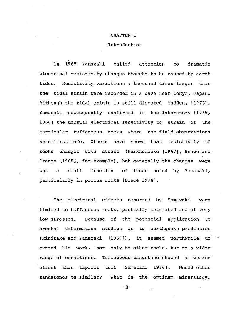
Samples of northern California tuffs were stressedwhile simultaneously measuring electrical resistance changesto investigate a phenomenon observed by Yanazaki on similarrocks from Japan. Resistance decreased substantially at lowstrain values for partially saturated samples. Strain wasamplified between 103 and 105 by the associated change inelectrical resistance.
The process was repeatable and recoverable in the tuffsunlike the behavior of other rock types. The principalfactors involved were porosity, Young's modulus and degreeof saturation.
A method is described to quickly sort out theelectrically amplifying tuffs from those that are not, as afirst step in locating a field site where this phenomenoncould be used as an earthquake monitoring technique.
Thesis Supervisor: William F. BraceProfessor of Geology
arkosic sandstone:52% quartz21% orthoclase20% calcite7% microclineopaque and lithicfragments
Navajosandstone
Pottsvillesandstone
sourceunknown
Springcity,Tenn.
16.4
3.0
8.5
7.5
99% quartz1% oxides
46% quartz41% orthoclase11% muscovite2% oxides
-45-
SANDSTONES
TB
76
AT BL
.8 110.2 17.2
10-
LINEAR
Figure Al
STRAIN
Stress-strain curves of Nevada/Montana tuffs
and the Pottsville and Berea sandstones
RM
14.2
FP
U)towHrU)
2
0
T UF F S
1BEREA SANDSTONE
4.7% Saturation
-0
0 1 2 3 4 5
STRESS, MpaChange in resistance with stress, TBT,
108
10
E0
z
Cnw
610
Berea ss.Figure A2
I 2 3 4 5 6STRESS MPa
-Figure A3 Change in resistance with stress:
-48-sandstones
108
E 6=100
z
4I-
104
BUTTE LAPILLI TUFF2
0
H
z
-
wjzcc
2 3 4 5 6 7 8
strain , C,
Figure A4 Relative change in resistivity with strain, BLT-49-
% SATURATION
0 I
Linear
cc
(e)4
w
0z
9% SATURATION
13
402740
I 2 3 4 5 6 7 8Linear strain, E , 10
Figure A5 Relative change in resistivity with strain,
Berea Sandstone
-50-
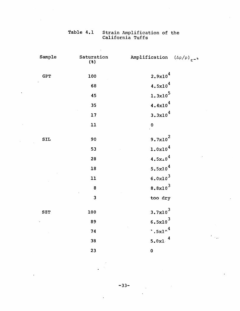
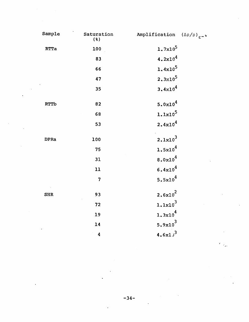
Strain Amplification of theMontana/Nevada Tuffs
Sample
BLT
RMT
TBT
Saturation(%)
4.2
5.0
5.2
11.2
12.6
29.6
49.1
2.5
4.7
5.1
5.4
38.0
45.0
2.8
4.8
7.3
9.9
12.9
20.1
46.8
-51-
Table A2
Amplification (AP/P) -4
2.3xl04
2.5x10³
1.6x10⁴
8.1x10³
2.1x10⁴
3.0x10³
2.8x10⁴
5. 0x102
0
5. 0x102
6.6x10²
1.0x10⁴
1.6x10⁴
7.0x10³
38.0x10
8.0x10³
1.0x10⁴
1.0x10⁴
4.4x10³
32.0x10
Sample Saturation Amplification (Ap/p)(%)
FPT 2.1 2.2x10³
3.8 1.2x10³
6.7 1.7x10³
15.2 3.2x10⁴
17.1 2.4xl03
22.2 8.8x10 4
58.0 8.0x10²
ATT 7.0 1.2x10²
11.1 1.3x10²
14.3 1.5x10 3
18.6 5.0x10²
56.0 1.0x10 4
-52-
Strain Amplification of Sandstones
Saturation(%)-
Mixed Company(Kayenta)
3.8
7.6
21.8
34.3
44.0
94.0
2.5
5.6
12.3
19.3
33.0
4.7
9.2
13.1
26.9
40.0
Amplification (Ap/p)
9.2x10²
4.0x10 2
1.0x10⁴
1.6xl03
. 3.1x10 3
2.4x10⁴
3. 2x10⁴
9 .2-:103
8.6x10 2
4.4x10 4
3.9x10 4
1. 2x10⁴
1. 6x10 3
9.1x10²
-53-
Sample
Navajo
Berea
Table A3
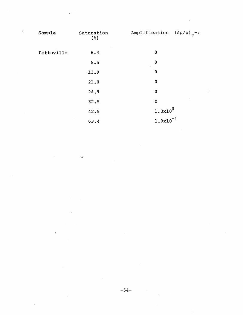
Sample Saturation Amplification (Ap/p) -4(%)
Pottsville 6.4 0
8.5 0
13.9 0
21.0 0
24.9 0
32.5 0
42.5 1.3x100
63.4 1.0x10 1
-54-
APPENDIX B
The Chunk Test
This test was devised to quickly investigate the
electrical properties of samples while still in a crude hand
specimen configuration. Results were strictly qualitative,
as the geometry factors of the irregular shapes were not
precisely known. However, chunk tests performed on the
Nevada and Montana tuffs showed that resistance cycled in
the same manner as the cylindrical samples described in
Appendix A, although to a lesser degree due to the larger
sample size. Therefore, the chunk test was indeed valid for
a preliminary sorting by electrical properties. Table Bl
lists the samples used in this test along with their
locations, and a brief hand specimen description.
Sample Configuration
Rock fragments were broken off into more or less equal
shapes about 5 cm long. Two lead sheets, 0.02 cm thick by
1.9 cm square were conformed on to opposite sides of the
sample, with copper wire soldered to each sheet, leading to
the resistance measuring circuit. The lead was epoxied
around the edges to the rock to avoid separation. The whole
assemblage was then. potted in Dow Corning Sylgard 186
-55-
silicone elastomer with the wires extending out of the
cylindrical case of rubber (Figure Bl).
Experimental Procedure
Potted samples were placed in a beaker of kerosene or
water inside a 15 cm diameter argon gas pressure vessel.
Kerosene is prefered to prevent corrosion of the vessel.
However, Sylgard swells in kerosene and the samples must
then be coated with Kenyon K-Kote to avoid expansion, a
process which adds a few days to the sample preparation.
Aesistances were measured at natural water content by
method 2 of Appendix D, while increasing and decreasing
hydrostatic pressure to a maximum of 5 MPa. The set-up is
schematically illustrated in Figure B2.
Data
Figures B3 through B5 show the electrical resistance
response to stress cycling on a number of the California
tuffs. Samples which exhibited little or no change are not
included. The unloading curves consistently fell below the
loading curves as with the cored rocks.
-56-.
Samples are ordered in terms of relative resistance
change in Table B2. Those with an asterisk were the ones
chosen for more detailed study. Some very sensitive rocks
were not selected because of their friability.
-57-
Table Bl
Sample Locati
PIN Pinnacles NMonument
SJB San Juan Gr(Salinas RdSan Juan Ba
COT Stony PointQuarry, Cot
CMV CoomsvilleNapa
MWT MontecelloNapa
SIL Silverado iSt. Helena
PET Petrified FRd., Calist
SIHR St. HelenaSt. Helena
DPR Deer Park RSunset Poir
Location and Hand Specimen Descriptionsof the California Tuffs
on Hand Specimen Description
ational Dense green tuff, numerous lithicfragments and phenocrysts
ade Rd. Conglomerate in tuffaceous matrix,.), pebbles up to 0.75 cm in diameterutista
Fine grained powdery grey clay inati 0.5 cm thick bed
Rd., Plum colored matrix, lithicfragments up to 1 cm, plagioclaselathes visible
Rd., Welded grey pumice fragments,light and porous
rail, White rhyolitic tuff, fragments ofwhite pumice up to 1 cm, lithicfragments (0.5 cm), plagioclaselathes
orest Rhyolitic tuff similar tooga Silverado, more weathered & friable
Rd., Coarse, grey, hard nd verycrystalline tuff, e: tensive andwell exposed in roa" cuts
d., .Very dense fine grained purple andt grey matrix with large pores; no
noticeable lithic fragments
-58-
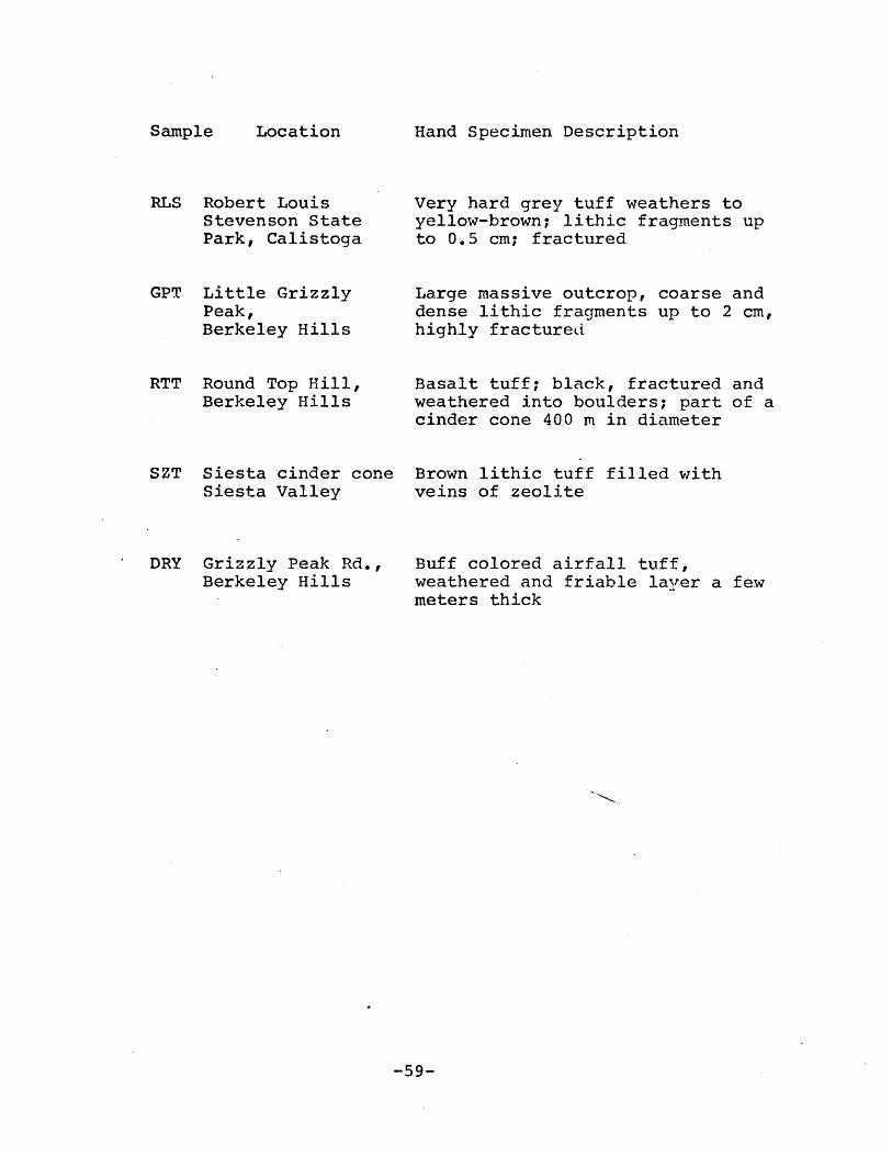
Hand Specimen Description
RLS Robert LouisStevenson StatePark, Calistoga
GPT Little GrizzlyPeak,Berkeley Hills
RTT Round Top Hill,Berkeley Hills
SZT Siesta cinder coneSiesta Valley
DRY Grizzly Peak Rd.,Berkeley Hills
Very hard grey tuff weathers toyellow-brown; lithic fragments upto 0.5 cm; fractured
Large massive outcrop, coarse anddense lithic fragments up to 2 cm,highly fractured
Basalt tuff; black, fractured andweathered into boulders; part of acinder cone 400 m in diameter
Brown lithic tuff filled withveins of zeolite
Buff colored airfall tuff,weathered and friable laver a fewmeters thick
-59-
Sample Location
copper wire
lead sheet
sample
rubber
Figure Bl Sample configuration for the chunk test
F.igure B2 Chunk test experimental apparatus
-60-
I 2 3 4 5
STRESS MPo
Figure B3 Change in resistance with stress;
SHR, DPR, RLS, DRY.
-61-
0
E
(nC0
w'
106
tnE.c:0
w
. 10
O-
I 2 3 4 5 6
STRESS MPo
Figure B4 Change in resistance with stress;
MWT, SZT, GPT.
-62-
1 2 3 4 5 6
STRESS MPa
Figure B5 Change in resistance with st--ess;
SJB, SIL, RTT, COT.
-63-
10
(n
E0
wz(n(nw
Table B2
Good
COT
DRY
GPT*
RTT*
Relative Ordering of Electrical Propertiesof California Tuffs
Fair
SZT*
RLS
DPR*
SIL*
Poor
SHR*
SJB
MWT
No Effect
CMV
PET
PIN
* Studied in detail
-64-
APPENDIX C
Stress-Strain and Electrical Behavior of
Selected California Tuffs
This section contains the complete set of data on the
California tuffs that were not included in chapter 4, as
they are similar to the examples shown there. Stress-strain
curves for the six tuffs are illustrated in Figure Cl.
Figures C2 and C3 show the change in resistance with stress
for each sample at an arbitrary saturation. The curves were
chosen to show the most typical electrical recoverability of
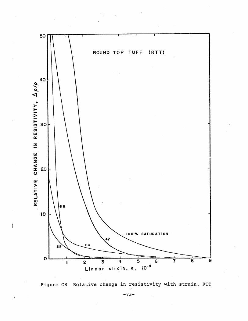
that sample. Figures C4 through C8 are plots of the
relative change in resistivity with strain and were derived
from the stress-strain and resistance data.
-65-
RTT GPT DPR SIL
LINEAR STRAIN
Figure Cl Stress-strain relation for the California tuffs
SHR0.
(n)
(14
U)4
2
0
SZT
10-3
GPT 35% Saturation
SIL 18 % Saturation
SHR 10 % Saturation
I 2 3 4 5 6STRESS MPa
Figure C2 Change in resistance with stress;
GPT, SIL, SHR.-67-
108
07
106
05
106 DPR 10% Saturatiorz
SZT 74 % Saturatio
105
RTT 90% Saturati
1041 2 3 4 5 6
STRESS MPa
Figure C3 Change in resistance with stress;
DPR, SZT, RTT
$20
Q-
15C:
10
5
45 % SATURATIONz8
35 35
2 4 6 8Linear strain, c , >0
Figure C4 Relative change in resistivity with strain, GPT
-69-
ST. HELENA ROAD (SHR)
4
-
zWz
26 % SATURATION
10
73
0 10 20 30Linear strain, E , 10
Figure C5 Relative change in resistivity with strain, SHR
-70-
12
10
mCC
z 6
(Dz
-
-
2- 38% SATURATION
010 20 30Linear strain, C 4
Figure C6 Relative change in resistivity with strain, SZT
-71-
12
DEER PARK ROAD (DPR)
10
8
(D)
z6
-Jw 4
31 7% SATURATION
2 75
95
0 2 4 6 8 10 12 14 16 18Linear strain, E 104
Figure C7 Relative change in resistivity with strain, DPR
-72-
50
40
m30
z
zr20
m
66
10
100% SATURATION
47
583I0'
I 2 3 4 5 6 7 8 9
Linear strain, e, 10
Figure C8 Relative change in resistivity with strain, RTT
-73-
APPENDIX Dl
Resistance Measuring Techniques
There are several techniques for measuring the
resistance of a rock, each with trade-offs on ease and
accuracy. Most of these methods involve matching the
voltage across a variable resistance decade with that across
the rock sample. In all cases, the source voltage was kept
at 10 Hz AC, to minimize any frequency effects that could
occur at higher frequencies. See Appendix D2 for a nore
complete description of frequency effects.
Method- 1.
Rrock
V. ti/ M Vin B
Rbox M VA
The particular circuit used for the early work on the
Nevada and Montana tuffs was the same as that in Brace,
Orange and Madden, [1965]. VA and VB are measured on a
vacuum tube volt meter (HP model 40011). From the above
circuit diagram, it follows that V =VB and the system is a
voltage divider where
VA RoxV. R + Rin rock box
Since Rb is known and a particular VA/V. is chosen,
then Rrock can be calculated. To simplify the calculation,
assume that Rbox is much less than Rrock , by appropriately
adjusting the voltage ratio.
V.Now Rrock = Rbox VA
The ratio VA /Vin is determined to make the resistance fall
in a reasonable range on the decade box and to introduce no
significant errors. For example, with Vin /VA lo0
Rrock = 100R box (Turn the voltmeter range down by two
orders of magnitude to measure VA , then adjust the decade
until the meter needle comes to the same point as it did for
VB)-
A 1% theoretical error is introduced because
Rexact rock =99Rbox * The difference is considered
negligable. By turning the voltage down in this manner, it
is possible to measure rock resistances that are greater
than the resolution of the variable resistance decade.
The advantage of this technique is that it is quick and
requires no calculation. In order to find t'e resistance of
the rock, one need only add two orders of mi nitude on to
the resistance read off the decade box. Most of the Nevada
and Montana tuff samples were measured in this way.
-75-
Problems: Since the signal to be measured on the meter
has been reduced substantially, there is a potential problem
of noise dominant errors. In fact if V /Vin = 1000, the
signal to noise ratio is high enough that the measured
resistance of the rock will have a noticeably large error
(as much as a factor of 10). In the noise dominant
situation, if V /V. is chosen to be 1/10 instead of 1/100A in
or 1/1000, then the signals are larger and the resistance
box gives better resolution. The exact formula for
Rrock must be used, otherwise there is a 10% error:
Rrock 9Rbox'
On the practical side, this choice of VA/Vin is not as
quick, as it requires more mental gymnastics to calculate 9R
than 10R. However, it is more accurate.
If the resistance of the decade, which has a maximum of
1 megohm, approaches the input impedance of the meter, then
the effective resistance is reduced:
1 =1 + 1
Reffective Rbox meter
R = Rbox . Rmetereffective Rbox + Rmeter
The effective value is substituted into the R values:
VA Rbox VA Reffective7 R + R becomes - R + Rin rock box in rock effective
The HP 400H voltmeter has an input impedance of roughly
2.5 megohms. This impedance is rather low and should be
taken into account when dealing with dry rocks whose
resistance can be as high as 10 megohms.
Method 2.
+ +
in M- box R rock _
R F
Method 2. involves the same technique of matching
voltages as method 1. A voltage is chosen with the switch
on R rock Then with the switch on Rbox, the resistance is
adjusted until the same voltage is obtained as through the
rock. Now Rrock=Rbox* An additional resistor RF is
necessary in this circuit otherwise Vmeter always equals
Vin*
Choice of RF: To find a suitable value of RF , the
sensitivity of the meter is analyzed with respect to the
power transfer between the circuit and the load (rock). By
Joule's Law, 22 ____R V Rr
pR +Rr r (1 + RF / Rr 2
-77-
According to this equation, the power in the load is zero if
the resistance of the rock is either very small, or very
large. Thus there must be some optimum value where the
power is a maximum. Differentiate and equate to zero:
dP 2 2R /R 2rock _ V F r + V - 0dR R ~ l+RR 3 (lRR 2 R2
- rock rock (1 + RF/Rr) (1 + RF/Rr) RF
2R RF = 1+ F
R R -rock rock
RF = rock
Therefore, a value of RF should be chosen that is close
to the expected value of R for maximu. sensitivity~ ofrock
the meter (greater accuracy 'in matching voltages). This
method was used in the "chunk tests" on the California tuffs
mainly because it is fast, and a switching box (R =1 megohm)
was readily available courtecy of D. Johnston.
A problem arises when Rrock is greater than the maximum
Rbox, mainly low saturation rocks. If the vnltage range of
the meter is switched down as in method 1, the same
simpiifying assumptions can not be made.
-78-
RkV. ( rock
in Rrock + RF Ml
Rb MV ( boxin Rbox + R F t M2
if V Ml = 0VM2' then
R rockRrock +KRF
= 100Rbox
Rbox + RF
RrockRbox + RrockRF = 100RboxRrock + 100 RboxRF
Rrock (RF - 99Rbox
R1OR -9 RR100boxRF-rock RF -99Rbox
Since RF = 106 ohms,
then
100 RboxR F
This is true if Rmeter is much greater than Rrock'
Otherwise the same problem with a low impedance meter exists
because the meter is in parallel with the rock and the box.
-79-
box effective ox
'rock effective Rrock equation in box
As can be seen from the above discussion, the switching
box method is no longer quick when trying to measaure high
impedance rocks.
Method 3.
V.in VB
Bridge method: RA and RB are fixed resistors.
adjusted until the bridge is balanced, i.e. the meter reads
zero volts. Then VA=VB'
VA RAV. R + Rin A box
RB
R + RB rock
VB
V.in
RA (RB + R ) = R(R + RR( +Rrock B A box
rock R A box
-80-
1
meter
Ret1mete
Rbox is
Note that the response does not in any way depend on
the meter. The ratio of RB to RA is chosen co scale Rbox to
Rrocke For instance, if Rrock max = 1 megohm and
Rbx max = 1 megohm, then make RB/RA =10. Now resistance
measurements greater than Rbox can be made. The absolute
magnitudes of RB and RA are set to gain the maximum meter
sensitivity to the null. RB is chosen to be around the same
order of magnitude as R rock. (See sensitivity derivation in
method 2). Then RA~ 100 kilohm for a typical low saturation
rock. This value is optimum for the decade box, since it
has maximum resolution in the middle ranges.
Because the resistance of the rock can vary widely
depending on the mineralogy and degree of saturation, say
between 1 kilohm and 10 megohm, it may be best to have two
sets of resistors for optimum sensitivity. Each set has
appropriate values of RA . This modification is not
tremendously important to the workings of the circUit unless
there is reason to be concerned with sensitivity.
RB = 10 kilohm for 1 kilohin<R rock<100 kilohm
and RB = 1 megohm for 100 kilohm<R rock<1 megohm
The bridge method has a definite advantage over the
other two methods. Since the meter does not enter into any
calculations, there are no errors due to low input impedance
or noise.
-81-
A problem common to all techniques: The source for the
resistance measuring circuit has an alternating current of
10 Hz. The strain gauge and corresponding circuit on the
other hand runs on DC, and is designed to detect small
changes in the DC voltage. Since the AC and DC currents are
juxtaposed in the sample, there is a coupling in which the
AC current appears in the strain signal. The epoxy between
the rock and strain gauge is not always enough to ensure
proper insulation, particularly with saturated samples. The
result is a 10 Hz vibration of the pen along the strain axis
as much as 2 cm wide, (leading to a mighty fuzzy
stress-strain curve!).
There are two solutions:
1) Disengage the pen while making a resistance measurement.
This tends to slow down the experiment, since there are
thirteen measurements to be made on each run, therefore
twenty-six times to flick the pen. The chance for human
error arises since one sometines forgets to engage the pen
after a measurement, and part of the stress-strain curve is
lost.
2) Build a low pass filter into the chart input. A somewhat
detailed description of the filter is in order as it has a
significant effect on the chart response.
-82-
FILTER
A standard low pass filter has response
V (s)
VCiu (s) 1 + sRCin
s= complex frequency 2TrfR= resistanceC= capacitance
Log ( ) v -0 2inin
Log s
Above some cutoff s=l/RC, the response drops by 20
db/decade. (i.e. V0 /Vin goes as l/s) . Since it is not
advantageous to vary s, for reasons stated in Appendix D3, R
and C are chosen such that 10 Hz is well above the cutoff,
On the other hand, if the cutoff is too low, the pen will
respond sluggishly since the filter causes a time delayed
response which goes as e-t/T
-83-
input
chart
output
Thus if the strain is changed quickly (say
instantaneously), the pen will not quite catch up to the
true value of strain and the stress-strain curve will be
slightly incorrect. This is a real problem because 10 Hz is
quite a low frequency. There are tight constraints imposed
on Tmax, where 10 Hz is just at the break point of the
response curve, and T min , a value that will not cause
noticEble delay in the pen.
The solution is to make sure that the stress is not
pumped up or released too fast, to allow time for the
delayed response. This introduces the question of strain
rate dependance of the system as a whole. The point of the
experiment is not to include strain rate as a parameter.
However, running a relatively slow test for response reasons
goes hand in hand with the fact that there must be time
allowed for the rock to equilibrate to the new stresses.
The pore water must redistribute, a factor dependant on
permeability.
-8.4-
Note that if the experiment were run at a higher
frequency, then "sluggishness" could be avoided altogether.
When the amplitude of the noise is low, a smaller capacitor
can be used to alleviate the response problem. At even
higher frequencies, say 10 k1z, the pen will not even have
time to respond to the noise.
Both solutions to the noise problem have their
disadvantages. One might wonder why the resistance is not
measured with DC. This would require the actual movement of
ions through the sample. If it is assumed that the charge
is being transmitted primarily by the water phase rather
than by mineral conduction, then a DC current would tend to
electrolyze the water. At one of the electrodes there would
be dissociated water forming oxygen and hydrogen gas. This
is far from a desirable situation, especially since fixed
partial saturation is an important factor in the experiment.
-85-
APPENDIX D2
Choice of Electrode Material
The ideal electrode material for measurina resistance
should have the following qualities:
1) Be a good conductor.
2) Maintain a good electrical contact with the sample
3) Have no stress effect (change in measured resistance with
applied stress) .
4) Have no frequency effect, or at least no frequency effect
within a given working range.
Four different electrode combinations were tested with
a 20 kilohm resistor in the following configuration:
Piston
+-Teflon a) lead sheet_ 4Metal
'r'-Wet paper b) lead sheet + wet layerWesterlyGranite c) copper sheet
20K20K__ -Paper d) copper sheet + wet layer
+-Metal
Base Teflon
The wet layer of paper is included to -ensure better
electrical contact to the rock. Results tend to be
inconsistent, because as the paper dries, the resistance
increases. The copper was annealed before testing to reduce
-8.6-
strain hardening effects, and enable the sheet to conform
better to the rock surfaces. However, as the copper is
stress cycled many times, strain hardening can become
permanent, even after annealing. The electrical conduction
properties of the copper lattice will vary slightly because
of distorted grains and dislocation pile-ups. This effect
will also cause the material to become less pliable.
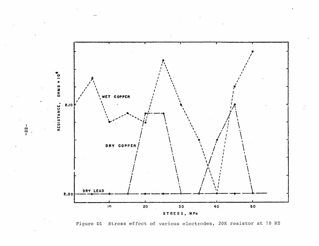
There appeared to be no significant frequency
dependance with the various electrode combinations, however
both the wet and dry copper in the stress test showed higher
resistance values than the correct value of 20 kilohms + 200
ohms (Figure Dl).
The dry lead sheet was chosen as the electrode
material. Lead is able to conform better to the surface of
the sample than the copper sheet, due to its low yield
stress. This is particularly important when testing
sandstones, which can have a very course surface. There was
no apparent stress effect with the dry lead.
-87-
T COPPER
.066I
9"
9'9'9'9'9'
9'.4
9'
9' j
I
"IAI 9'
/ '9',
It
DRY LEAD
40 50
S T R E S S , MPa
Figure Dl Stress effect of various electrodes, 20K resistor
'
WE
2.10
z
I-cc
DRY COPPER/
2.00
I0000I
at 10 HZ
APPENDIX D3
Freguency Effects
When dealing with high impedance rocks, second order
effects become important. This is particularly true over
the frequency spectrum. Consider a dry or partially
saturated rock between two copper wires. Because the rock
is so much less conductive than the wires, it has some of
the characteristics of a capacitor. A model of the system
could be represented as shown below.
.dVC i=C --
dt
R i=V/R
Since the current through the capacitor i=dV/dT C, then
at high frequencies, dV/dT will be large. As the current
through C increases with higher frequencies, there is
correspondingly less current through R. The meter reads a
smaller voltage across R, and hence a smaller R than the
true value. The actual response can be found by analyzing
ZR11 ZC
-89-
Z = R
ZC jfCR1 jf .1C jC
+ jfC = 1 jfR
Log Z
Z R1 + jfCR
Log f
When the frequency is small, Z=R, and when the frequency is
large Z falls off as 1/w. There will be a family of curves
for varying resistance.
The accuracy of standard film resistors at 107 ohms
breaks down at 100 Hz, therefore a frequency of 10-100 Hz is
suitable to eliminate the capacitance effects of the fixed
resistors in the electrical resistance bridcre of method 3.
The plot in Figure D2 was obtained using rocks of
varying saturation with no axial stress. The tuffs have a
high internal capacitance. Since the point of this
experiment is not to investigate the frequency dependance of
resistance in the tuffs, it is necessary to run the
frequency as low as possible to measure the high impedance
samples. Above 10 .ohms (at 10 Hz), the resistance values
are already on the sloping part of the response curve. Thus
they represent a minimrum resistance, and are a contributing
-90-
factor to the scatter in the data. Frecuencies of less than
10 Hz are not desirable due to the electrolyzing problems of
a DC-like current.
-91-
RTT (77)
GPT (45)
SZT (75)
E
0z
SZT (86% Sot.)
I:
10- sHR (58)
SIL (65)
S HR '(34)
lei00O', 102 103 04105
FREQUENCY (Hz)
Figure D2 Resistance fall-off with frequency for the
California tuffs at varying saturations
REFERENCES
Brace, W.F., Electrical resistivity of sandstoneFinal report to Defence Nuclear Agency, contract no.DNA-001-74-C-0057, 40p, 1974
Brace, W.F., Permeability from resistivity and pore shape,J. Geophys. Res., 82(23), 3343, 1977
Brace, W.F., and A.S. Orange, Electrical resistivity changesin saturated rocks during fracture and frictionalsliding, J. Geophys. Res., 73(4), 1433, 1968
Brace, W.F., A.S. Orange, and T.M. Madden, The effect ofpressure on the electrical resistivity of water saturatedcrystalline rocks, J. Geophys. Res., 70(22), 5669, 1965
Carozzi, A., Microscopic Sedimentary PetrologyJohn Wiler & Sons, Inc. New York, 1960
Madden, T.M., Electrical measurements as stress-strainmonitors, U.S.G.S. Office of Earthquake Studies.Proceedings of conference VII: Stress and strainmeasurements related to earthquake prediction. Openfile report 79-370; Menlo Park, California, 1978
Parkhomenko, E.I., Electrical Properties of RocksPlenum Press, New York 314p, 1967
Rik'itake, T. and Y. Yamazaki, Electrical conductivity ofstrained rocks: The fifth paper. Residual strainsassociated with large earthquakes as observed by aresistivity variometer.Bul. Earthrauake Res. Inst. 47, 99, 1969
Sprunt, E.S., and W.F. Brace, Direct observation of micro-cavities in crystalline rocks, Rock Mechanics and MiningSciences and Geomechanics Abstracts, 11(4), 371974
Stesky, R.M., and W.F. Brace, Electrical conductivity ofserpentinized rocks to 6 kilobars.J. Geophys. Res., 78(32), 1973
Yamazaki, Y., Electrical conductivity of strained rocks:The first paper. Laboratory experiments on sedimentaryrocks. Bul. Earthquake Res. Inst. 43, 783, 1965
Yamazaki, Y., Electrical conductivity of strained rocks:The second paper. Further experiments on sedimentaryrocks. Bul. Earthquake Res. Inst. 44, 1553, 1966