126
Semester thesis Theoretical Electricity Demand in ASEAN: Modeling and Forecasting Hajer Ben Charrada SA658 2016/10

Semester thesis
Theoretical
Electricity Demand in ASEAN:
Modeling and Forecasting
Hajer Ben Charrada
SA658
2016/10


Supervisors: Juergen Stich TUM Create Ltd Create Way 1 138602 Singapore Christoph Wieland Technische Universität München Lehrstuhl für Energiesysteme Boltzmannstr. 15 85748 Garching b. München Given out: 01.05.2016 Submitted: 30.10.2016


Eidesstattliche Erklärung
Hiermit versichere ich, die vorliegende Arbeit selbständig und ohne Hilfe Dritter angefertigt
zu haben. Gedanken und Zitate, die ich aus fremden Quellen direkt oder indirekt übernom-
men habe sind als solche kenntlich gemacht. Diese Arbeit hat in gleicher oder ähnlicher
Form noch keiner Prüfungsbehörde vorgelegen und wurde bisher nicht veröffentlicht.
Ich erkläre mich damit einverstanden, dass die Arbeit durch den Lehrstuhl für Energiesys-
teme der Öffentlichkeit zugänglich gemacht werden kann.
_________, den ___________ _______________________
Unterschrift


Abstract I
Abstract
A hybrid bottom-up (end-use) and top-down (econometric) power demand model is devel-
oped in order to deliver projections for the annual power demand and the corresponding
load profiles in hourly resolution. The model is applied for all ASEAN nations (10 countries).
The bottom-up model is applied to the residential sector, while the econometric model is
applied for the three other sectors (industry, service, other activities). As projection varia-
bles, the end-use model takes into consideration socio-economic (population, GDP, ur-
banization, electrification) as well as technology related (technology diffusion, efficiency
improvement) factors. The econometric model relies on the observation that specific power
consumption growth decreases gradually with increasing economic development. The cor-
relation is performed with time series data from different countries, and the projections
follow power functions. Power load profiles in hour resolution are generated from both
models for the total electricity consumption. The generated load profile comprises an
HVAC share, which is calculated in accordance with the meteorological characteristics of
the modeled region.
Key Words: energy modeling, demand forecasting, end-use, econometric, load profiles,
ASEAN
Abstract
Ein hybrides top-down/bottom-up Modell ist entwickelt, um Prognosen des jährlichen
Elektrizitätsverbrauchs und die entsprechenden stündlichen Lastprofile zu liefern. Das Mo-
dell ist für ASEAN Nationen (10 Länder) genutzt. Das Endverbrauch (bottom-up) Modell ist
für den privaten Sektor und das ökonometrische Modell (top-down) für die restlichen Sek-
toren (Industrie, Dienst, Andere Aktivitäten) angewendet. Beim Endverbrauchsmodell ge-
hören zu den Prognosevariablen die sozioökonomischen Größen (Bevölkerung, GDP, Ur-
banisierung, Elektrifizierung) sowie technologiebezogene Faktoren (Diffusion von Techno-
logien, Effizienzverbesserung). Das ökonometrische Modell basiert auf der Beobachtung,
dass das Wachstum vom spezifischen Elektrizitätsverbrauch mit steigender wirtschaftli-
cher Entwicklung sinkt. Die Korrelation ist durchgeführt mit Zeitreihendaten aus verschie-
denen Ländern, und die Prognosen folgen Potenzfunktionen. Stündliche Elektrizitätslast-
profile sind aus beiden Modellen für den Gesamtverbrauch generiert. Die generierten Last-
profile beinhalten einen Klimaabhängigen Anteil.
Schlagwörter: Energiesysteme Modellierung, Nachfrage Prognosen, Endverbrauch, Öko-
nometrie, Lastprofil, ASEAN

II Table of Contents
Table of Contents
List of Figures ....................................................................................................... IV
List of Tables ........................................................................................................ VII
1 Introduction ............................................................................................ 8
2 Understanding Energy Demand ............................................................. 10
2.1 Economic foundations of energy demand ........................................................ 10
2.2 Energy demand forecasting techniques ........................................................... 10
2.2.1 Time ranges of demand forecasting ......................................................... 11
2.2.2 Energy demand forecasting approaches .................................................. 11
2.3 Modeling energy demand in the context of developing countries .................... 15
2.3.1 Common background for developing countries ....................................... 15
2.3.2 Demand modeling for developing countries ............................................. 16
2.4 Dynamics of technological changes ................................................................. 17
2.4.1 Technology dynamics ............................................................................... 17
2.4.2 Technology diffusion and adoption ........................................................... 18
2.4.3 Technology transfer and diffusion in the context of developing countries
.................................................................................................................. 19
2.5 Structure of electricity supply ........................................................................... 20
2.5.1 Load-duration curve .................................................................................. 20
2.5.2 Load-curve projections ............................................................................. 22
3 An overview of ASEAN ........................................................................... 23
3.1 ASEAN’s economy ............................................................................................ 23
3.2 ASEAN’s energy landscape .............................................................................. 27
3.2.1 Primary energy .......................................................................................... 27
3.2.2 Power sector ............................................................................................. 28
3.2.3 Integration of renewables and trans-border electricity trade .................... 29
3.2.4 Power demand and projection in ASEAN: existing research .................... 30
4 Methodology .......................................................................................... 32
4.1 Bottom-up modeling ......................................................................................... 33
Table of Contents III
4.1.1 Concept and structure ............................................................................. 33
4.1.2 Location dependent share of the power consumption ............................ 35
4.1.3 Generating power load profiles ................................................................ 39
4.1.4 Demand forecasting ................................................................................. 40
4.2 Top-down modeling ......................................................................................... 47
4.2.1 Concept and structure ............................................................................. 47
4.2.2 Deriving power load profiles ..................................................................... 51
4.3 Projection scenarios ......................................................................................... 52
4.4 Limits of the modeling approaches .................................................................. 53
4.5 Data collection and sources ............................................................................. 53
4.5.1 Bottom-up model ..................................................................................... 53
4.5.2 Top-down model ...................................................................................... 55
4.5.3 Model validation ....................................................................................... 55
4.6 Modeling tools .................................................................................................. 56
5 Results and Discussion ......................................................................... 58
5.1 Model validation ............................................................................................... 58
5.2 Growth trends ................................................................................................... 59
5.3 Results from the bottom-up model for residential demand ............................. 61
5.3.1 Breakdown of residential power demand ................................................. 61
5.3.2 Urbanization and future trends ................................................................. 64
5.4 Results from top-down model and overall demand projection ........................ 66
5.4.1 Final demand estimates ........................................................................... 66
5.4.2 Scenario analysis ...................................................................................... 74
5.5 Generated power load profiles ......................................................................... 74
6 Conclusions ........................................................................................... 79
References ........................................................................................................... i
Appendices ............................................................................................................................. xiii
IV List of Figures
List of Figures
Figure 1 A simple case of technological substitution ....................................... 18
Figure 2 Penetration rates of appliances in China ............................................ 19
Figure 3 Sample system load curve for a Brazilian utility ................................. 21
Figure 4 Sample load-duration curve ............................................................... 21
Figure 5 Illustration of a residential load curve by different end-uses .............. 22
Figure 6 Population of ASEAN between 1990 and 2015 .................................. 24
Figure 7 Human Development Index of ASEAN members between 1990 and 2014 ....................................................................................................... 25
Figure 8 Urbanization rate of ASEAN members between 1990 and 2015 ........ 25
Figure 9 Per capita GDP of ASEAN member countries between 1990 and 2013 ....................................................................................................... 26
Figure 10 Fuel shares in primary energy demand in ASEAN, 2000 and 2013 .. 27
Figure 11 Primary energy overview of ASEAN countries .................................. 28
Figure 12 Generation mix of the ASEAN countries in 2013 .............................. 29
Figure 13 Comparative normalized load profiles in a typical day of Singapore and Laos ................................................................................................ 31
Figure 14 Global schema of the developed power demand projection model . 32
Figure 15 Black-box structure of the end-use model for residential power demand .................................................................................................. 33
Figure 16 Defined processes and household appliances for bottom-up modeling ................................................................................................ 35
Figure 17 Definition of the water heater factor 𝒅𝐰𝐡 ......................................... 38
Figure 18 Usage probability distribution for air-conditioner ............................. 40
Figure 19 Weibull CDF for different values of 𝜶 (𝜷 = 𝟑) and different values of 𝜷 (𝜶 = 𝟒) ................................................................................................ 42
Figure 20 Correlation data (brown) and result Weibull CDF (blue) for electrification rates in urban and rural areas .......................................... 43
Figure 21 Correlation data (brown) and result Weibull CDF (blue) for ownership of refrigerators (all households) ............................................ 44
Figure 22 Two different methods to adjust single data points to the overall curve (case of vacuum cleaner ownership rates) ................................... 46
List of Figures V
Figure 23 Example for regression data of the total final electricity consumption/cap as function of GDP/cap displayed in double logarithmic scale .................................................................................... 47
Figure 24 Correlation data for the industry sector, represented in double logarithmic scale .................................................................................... 49
Figure 25 Resulting estimates for service, industry and total consumption ..... 50
Figure 26 Load profile shapes (hour coefficients) ............................................ 52
Figure 27 Screenshot of the bottom-up Excel module .................................... 56
Figure 28 Workflow in the developed model software ..................................... 57
Figure 29 Population estimates until 2040 in ASEAN ....................................... 60
Figure 30 GDP per capita estimates until 2040 in ASEAN ............................... 60
Figure 31 Residential load breakdown in a weekday of the base year ............ 61
Figure 32 Residential load breakdown in a weekday, projection for 2040 ....... 62
Figure 33 Projection of air conditioner ownership rates in households ............ 63
Figure 34 Example of a weekday and a weekend load in Vietnam (base year) 64
Figure 35 Example of a weekday and a weekend load in Vietnam (2040, moderate scenario) ................................................................................ 64
Figure 36 Evolution of rural and urban households in Thailand and Indonesia, and their respective contribution to the residential power demand ...... 65
Figure 37 Overall final demand projections for Malaysia (moderate scenario) . 66
Figure 38 Overall final demand projections for Singapore (moderate scenario)66
Figure 39 Overall final demand projections for Indonesia (moderate scenario) 67
Figure 40 Overall final demand projections for The Philippines (moderate scenario) ................................................................................................ 67
Figure 41 Overall final demand projections for Brunei (moderate scenario)..... 68
Figure 42 Overall final demand projections for Thailand (moderate scenario) . 68
Figure 43 Overall final demand projections for Myanmar (moderate scenario) 69
Figure 44 Overall final demand projections for Cambodia (moderate scenario)69
Figure 45 Overall final demand projections for Vietnam (moderate scenario) . 70
Figure 46 Overall final demand projections for Laos (moderate scenario) ....... 70
Figure 47 Final electricity demand in ASEAN: history and estimates ............... 72
Figure 48 Sectors contribution to the final electricity demand estimates in 2015 and 2040 ....................................................................................... 73

VI List of Figures
Figure 49 Demand scenarios for the whole ASEAN region .............................. 74
Figure 50 Example load profiles of Vietnam (2015) and Malaysia (2015) ......... 75
Figure 51 Comparison between the load profile for Singapore and Cambodia 76
Figure 52 Generated load profile of The Philippines in 2015 (left) and in 2040 (right) ...................................................................................................... 77
Figure 53 Correlation between power load and temperature ........................... 78

List of Tables VII
List of Tables
Table 1 Used methods for input variables projection (bottom-up modeling) ... 41
Table 2 Defined categories for household appliances ..................................... 44
Table 3 Assumptions regarding appliances ownership projection ................... 45
Table 4 Country clustering definition according to Human Development Index HDI ......................................................................................................... 48
Table 7 Definition of projection scenarios ........................................................ 53
Table 5 Summary of data used in bottom-up model ....................................... 54
Table 6 Electricity consumption and load profile data sources ........................ 56
Table 8 Bottom-up model demand output for the base year compared to real demand .................................................................................................. 58
Table 9 GDP average annual growth rates (aagr) in ASEAN ............................ 59
Table 10 Population average annual growth rates (aagr) in ASEAN ................. 59
Table 11 Final electricity demand average annual growth rates (aagr) ............ 71
8 1.1
1 Introduction
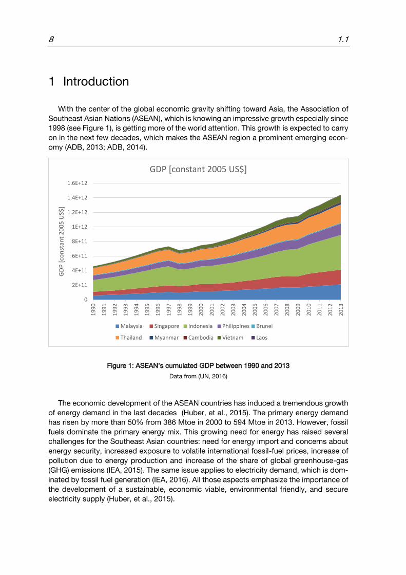
With the center of the global economic gravity shifting toward Asia, the Association of
Southeast Asian Nations (ASEAN), which is knowing an impressive growth especially since
1998 (see Figure 1), is getting more of the world attention. This growth is expected to carry
on in the next few decades, which makes the ASEAN region a prominent emerging econ-
omy (ADB, 2013; ADB, 2014).
Figure 1: ASEAN’s cumulated GDP between 1990 and 2013
Data from (UN, 2016)
The economic development of the ASEAN countries has induced a tremendous growth
of energy demand in the last decades (Huber, et al., 2015). The primary energy demand
has risen by more than 50% from 386 Mtoe in 2000 to 594 Mtoe in 2013. However, fossil
fuels dominate the primary energy mix. This growing need for energy has raised several
challenges for the Southeast Asian countries: need for energy import and concerns about
energy security, increased exposure to volatile international fossil-fuel prices, increase of
pollution due to energy production and increase of the share of global greenhouse-gas
(GHG) emissions (IEA, 2015). The same issue applies to electricity demand, which is dom-
inated by fossil fuel generation (IEA, 2016). All those aspects emphasize the importance of
the development of a sustainable, economic viable, environmental friendly, and secure
electricity supply (Huber, et al., 2015).
0
2E+11
4E+11
6E+11
8E+11
1E+12
1.2E+12
1.4E+12
1.6E+12
19
90
19
91
19
92
19
93
19
94
19
95
19
96
19
97
19
98
19
99
20
00
20
01
20
02
20
03
20
04
20
05
20
06
20
07
20
08
20
09
20
10
20
11
20
12
20
13
GD
P [
con
stan
t 2
00
5 U
S$]
GDP [constant 2005 US$]
Malaysia Singapore Indonesia Philippines Brunei
Thailand Myanmar Cambodia Vietnam Laos
Chapter 1 Introduction 9
The Southeast Asian region offers abundant sources of renewable energies, which are
not anywhere utilized near to their potential. More-over, the renewable energy sources are
unevenly distributed across the ASEAN region (WEC, 2010; Lidula, et al., 2007). Trans-
border electricity trade and the development of a common ASEAN power grid offer the
opportunity to maximize the benefit from integrating renewable energies and reduce total
exploitation costs (Chang & Li, 2012; Kutani & Li, 2014; Huber, et al., 2015; Stich & Massier,
2015).
The development and optimization of such a system requires knowledge about the sup-
ply side in terms of renewable energy sources, as well as the demand side and its devel-
opment in the future. Due to the volatility of renewable energy sources, the exact
knowledge about the demand side up to higher resolution in time is necessary. The aim of
this work is to develop an electricity demand model, which enables to deliver future pro-
jections for the total electricity demand at the national level as well as derivate the corre-
sponding power load profiles in hourly resolution.
The second chapter describes the theoretical background of energy demand modeling
in general and the specific case of electricity demand, and also deals with the different
specificities of the studied problem as technological changes and modeling in developing
countries. The third chapter presents a general overview of the ASEAN region in terms of
economic situation and energy system. The fourth chapter describes in detail the devel-
oped model within this work with its different modules. The last chapter presents the re-
sults obtained from the modeling and discusses them.
1.1

10 2.1 Economic foundations of energy demand
2 Understanding Energy Demand
Energy demand arises to satisfy needs which are met using certain technological appli-
ances. Hence, demand for energy depends of the choice of services to meet those needs.
The end-use service demand depends itself on the energy cost and availability and also
on other factors like climatic conditions, income (of decision maker), cultural aspects etc.
The dynamics of energy demand is highly dependent of the inertia of appliance stocks.
The stocks usually can change over a long period of time, and this can be due to economic
or behavioral factors.
Energy demand analysis tries to consider these aspects in different ways: the econo-
mists’ approach relies on optimizing behavior based on the neoclassical tradition of eco-
nomics, while another approach inspired from engineering traditions focuses on the de-
mand processes introducing behavioral factors (such as meeting user needs or technolog-
ical changes). This divergence of methods let to the appearance of two distinct traditions
in energy analysis literature: the econometric (top-down) approach and the engineering
end-use (bottom-up) approach (Bhattacharyya & Timilsina, 2009).
This chapter explores the theoretical background of energy demand forecasting pre-
senting the different methods and classifications in sections 2.1 and 2.2. The context of
developing countries for energy demand modeling is analyzed in paragraph 2.3. Section
2.4 discusses one of the most important variables for energy demand which is technology
change dynamics. And the last section 2.5 states the specificities of electricity demand as
a special form of energy.
2.1 Economic foundations of energy demand
The factors driving energy demand differ between economic sectors. Industries and
service users consider energy as an input of their overall cost-function which they tend to
minimize in order to optimize production costs (producer theory). Households, however,
use energy to satisfy certain needs -among other competing needs- by allocating part of
their income in order to reach a certain degree of satisfaction within their expenditure (con-
sumer theory). (Bhattacharyya & Timilsina, 2009)
The motivation for energy use differs therefore between these two groups, and they
should be treated separately.
2.2 Energy demand forecasting techniques
An array of methods has been developed so far for energy demand forecasting, and
different literature presents several ways to classify those methods based on time range,
model type, sophistication level etc.

Chapter 2 Understanding Energy Demand 11
2.2.1 Time ranges of demand forecasting
Depending on the time window of the study, forecasting methods can be arranged in
three categories (Al-Alawi & Islam, 1996)
2.2.1.1 Short-term forecasting
These methods aim to periods from few hours to few weeks. They play an important
role in day-to-day operations of a utility such as for unit commitment, load management,
economic dispatch etc. This type of forecast determines the hourly demand load.
2.2.1.2 Medium-term forecasting
These forecasts aim to a time-range from few weeks up to few years. They are neces-
sary for planning fuel procurement, scheduling unit maintenance, energy trading and rev-
enue assessment etc. This type of forecast determines monthly loads.
2.2.1.3 Long-term forecasting
Long-term forecasts are usually valid from 5 to 25 years. They are important in making
decisions about transmission expansion/upgrade plans, integration of new power plants,
implementation of energy specific strategies etc. This type of forecast is commonly known
as an annual peak load and energy forecast.
(Al-Alawi & Islam, 1996)
In the following, we will consider only long-term forecasting techniques since it is the
aim of this study.
2.2.2 Energy demand forecasting approaches
As mentioned in the beginning of this section, two main approaches marked the energy
demand analysis literature: econometric and end-use. (Werbos, 1990) presents the differ-
ence between the different modeling approaches with a simple example:
We want to forecast a population POP (t ) in the year t +1 based on the year t infor-
mation. We can write the following equation:
𝑃𝑂𝑃(𝑡 + 1) = 𝑐 ∙ 𝑃𝑂𝑃(𝑡)
Where c is a constant.
“If the value of c is obtained by asking the boss, the forecast is based
on the judgmental approach. If c is obtained through small-scale studies
of controlled population, the model can be called an engineering model.
If c is obtained by analyzing the time series of historical population, the
model can be called an econometric model or a model estimated using
the econometric approach.”
(Werbos, 1990; Bhattacharyya & Timilsina, 2009)

12 2.2 Energy demand forecasting techniques
2.2.2.1 Econometric approach
An econometric approach is a standard quantitative method which combines economic
theory with statistical consideration to establish a relationship between the dependent var-
iable (in our case electricity demand) and certain independent variables (weather, socio-
economic and demographic variables). The correlation between dependent and independ-
ent variables can be established considering time-series and/or cross-sectional data. The
selection criterion of the independent variables could be based on human intuition, and
will be finally validated by their correlation level. Inserting forecasts of the independent
variables into the resulting equation would yield the energy demand projections. This ap-
proach can be applied to total aggregated energy as well as individual sectors (Al-Alawi &
Islam, 1996; Bhattacharyya & Timilsina, 2009; Mehra & Bharadwaj, 2000)
According to (Swisher, et al., 1997), the most common type of econometric equation
used in energy demand prediction is based on the Cobb-Douglas production function
𝐸 = 𝑎𝑌𝛼𝑃−𝛽
Where:
𝐸 : the energy demand
𝑌 : income
𝑎 : coefficient
𝛼 : income elasticity of energy demand
𝛽 : price elasticity of energy demand
Income and price elasticities indicate how the demand for energy changes as a result
of change in income and price respectively.
𝛼 = ∆𝐸
𝐸⁄
∆𝑌𝑌⁄
, 𝛽 = ∆𝐸
𝐸⁄
∆𝑃𝑃⁄
The parameters a, α and β can be estimated using past data series and statistical meth-
ods (e.g. regression analysis) (Swisher, et al., 1997)
There is a wide range of methods and models for econometric forecasting which use
either statistical techniques or artificial intelligence algorithms (e.g. regression, stochastic
time series, fuzzy logic and neural networks). Several literatures show an extensive over-
view of the different methods: (Alfares & Nazeeruddin, 2002; Hahn, et al., 2009; Berk,
2015; Chen, et al., 2001; Feinberg & Genethliou, 2005)
The econometric models require a consistent set of data over a reasonably long period
of time. However, the fundamental assumption of this method is that the correlation be-
tween dependent and independent variables will continue to hold in the future. It doesn’t
analyze therefore the fundamental structure of energy supply and demand and fails to cap-
ture certain endogenous factors like policy measures, economic shocks, technological
changes and consumer behavior. (Mehra & Bharadwaj, 2000; Swisher, et al., 1997)
Chapter 2 Understanding Energy Demand 13
2.2.2.2 End-use approach
As its name may suggest, the end-use approach or engineering-economy approach
focuses on end-uses or final needs of the consumer at a disaggregated level. It is based
on a more detailed model than the econometric approach, though its analytical formulation
can be quite simple. The estimates are derived from modeling directly the consumer struc-
ture including (electric) appliances, customer use, socio-economic factors, energy pene-
tration etc. Statistics about the end-users as well as dynamics of socio-economic and
technological changes are base for the forecast. (Bhattacharyya & Timilsina, 2009;
Feinberg & Genethliou, 2005; Swisher, et al., 1997)
According to the models developed by the United Nations and the International Atomic
Energy Agency (UN, 1991; IAEA, 2006) based on the theory of (Chateau & Lapillonne,
1978), the general procedure involves:
1. Disaggregation of total energy demand into homogeneous end-use modules (e.g.
economic sectors)
2. Organization of end-uses into a hierarchical structure of processes
3. Formalization of the structure in a mathematical model
4. Modeling of the reference year:
a. Reference year is taken as the most recent year for which data is available
b. Basic foundation of the whole model and the forecasts
5. Analysis of socio-economic and technological factors to determine interrelation-
ships and hence long-term evolution
6. Scenario design for the future based on 5.
7. Quantitative forecasting using mathematical relations and scenarios
(Bhattacharyya & Timilsina, 2009)
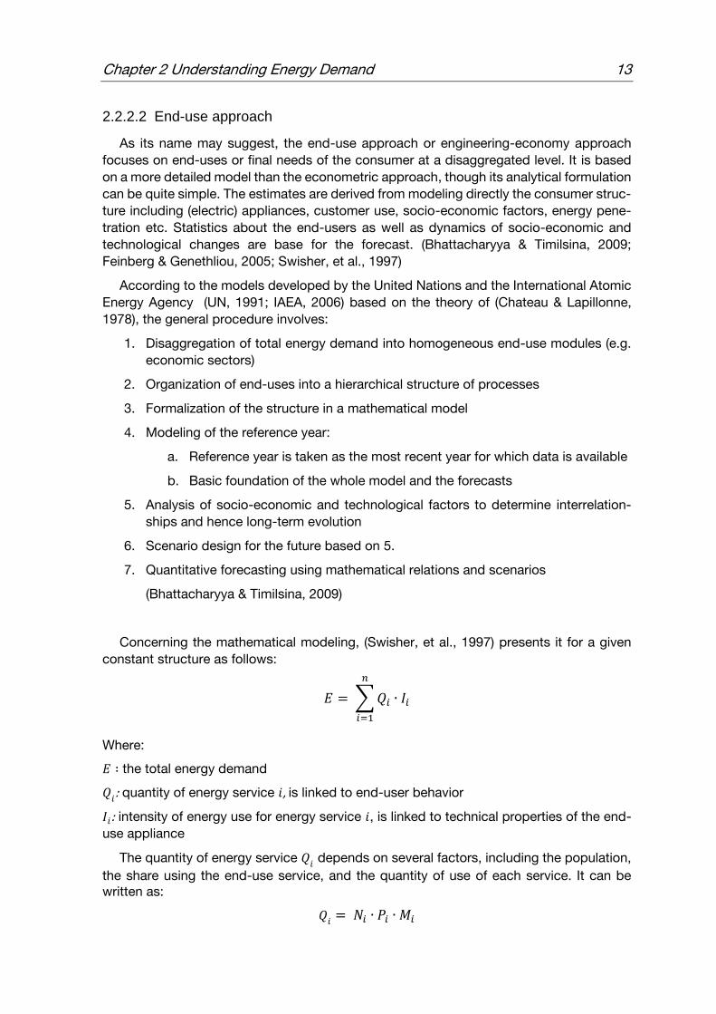
Concerning the mathematical modeling, (Swisher, et al., 1997) presents it for a given
constant structure as follows:
𝐸 = ∑ 𝑄𝑖 ∙ 𝐼𝑖
𝑛
𝑖=1
Where:
𝐸 ∶ the total energy demand
𝑄𝑖: quantity of energy service 𝑖, is linked to end-user behavior
𝐼𝑖: intensity of energy use for energy service 𝑖, is linked to technical properties of the end-
use appliance
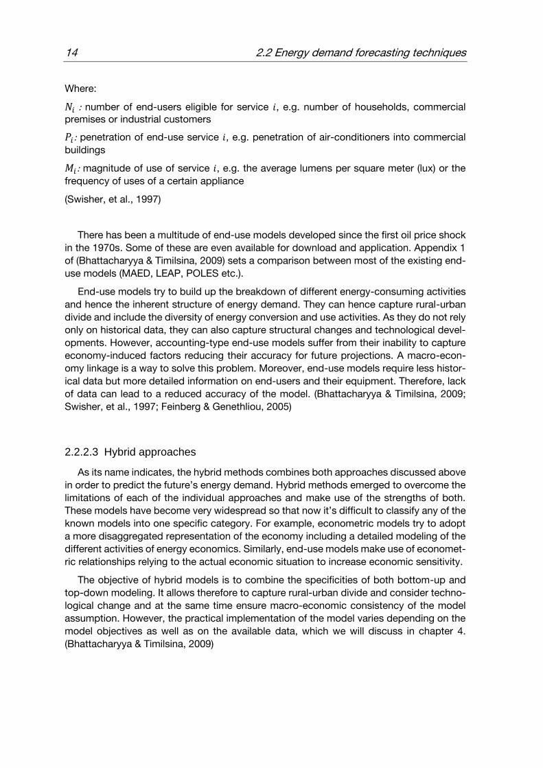
The quantity of energy service 𝑄𝑖 depends on several factors, including the population,
the share using the end-use service, and the quantity of use of each service. It can be written as:
𝑄𝑖 = 𝑁𝑖 ∙ 𝑃𝑖 ∙ 𝑀𝑖
14 2.2 Energy demand forecasting techniques
Where:
𝑁𝑖 : number of end-users eligible for service 𝑖, e.g. number of households, commercial premises or industrial customers
𝑃𝑖: penetration of end-use service 𝑖, e.g. penetration of air-conditioners into commercial
buildings
𝑀𝑖: magnitude of use of service 𝑖, e.g. the average lumens per square meter (lux) or the
frequency of uses of a certain appliance
(Swisher, et al., 1997)
There has been a multitude of end-use models developed since the first oil price shock
in the 1970s. Some of these are even available for download and application. Appendix 1
of (Bhattacharyya & Timilsina, 2009) sets a comparison between most of the existing end-
use models (MAED, LEAP, POLES etc.).
End-use models try to build up the breakdown of different energy-consuming activities
and hence the inherent structure of energy demand. They can hence capture rural-urban
divide and include the diversity of energy conversion and use activities. As they do not rely
only on historical data, they can also capture structural changes and technological devel-
opments. However, accounting-type end-use models suffer from their inability to capture
economy-induced factors reducing their accuracy for future projections. A macro-econ-
omy linkage is a way to solve this problem. Moreover, end-use models require less histor-
ical data but more detailed information on end-users and their equipment. Therefore, lack
of data can lead to a reduced accuracy of the model. (Bhattacharyya & Timilsina, 2009;
Swisher, et al., 1997; Feinberg & Genethliou, 2005)
2.2.2.3 Hybrid approaches
As its name indicates, the hybrid methods combines both approaches discussed above
in order to predict the future’s energy demand. Hybrid methods emerged to overcome the
limitations of each of the individual approaches and make use of the strengths of both.
These models have become very widespread so that now it’s difficult to classify any of the
known models into one specific category. For example, econometric models try to adopt
a more disaggregated representation of the economy including a detailed modeling of the
different activities of energy economics. Similarly, end-use models make use of economet-
ric relationships relying to the actual economic situation to increase economic sensitivity.
The objective of hybrid models is to combine the specificities of both bottom-up and
top-down modeling. It allows therefore to capture rural-urban divide and consider techno-
logical change and at the same time ensure macro-economic consistency of the model
assumption. However, the practical implementation of the model varies depending on the
model objectives as well as on the available data, which we will discuss in chapter 4.
(Bhattacharyya & Timilsina, 2009)

Chapter 2 Understanding Energy Demand 15
2.3 Modeling energy demand in the context of developing countries
Bhattacharya et. al argue that the existing energy demand forecasting methodologies
are not well suited for the developing countries context and do not reflect specificities of
those countries (Bhattacharyya & Timilsina, 2009; Bhattacharyya & Timilsina, 2010). This
section will point out the features of developing countries and what should be considered
when modeling their energy structure.
2.3.1 Common background for developing countries
Although there is a wide diversity between developing economies regarding socio-eco-
nomic properties (e.g. economic structure, urbanization level, human development etc.),
some common traits of the energy system can be deduced (OTA, 1991). According to
(Bhattacharyya & Timilsina, 2010), these characteristics include:
Reliance on traditional energies
The existence of large informal sectors
Urban-rural divide and the prevalence of poverty and inequity
Structural changes of the economy and accompanying transition from traditional
to modern life style
Inefficient energy sector characterized by supply shortages and poor perfor-
mance of energy utilities
Existence of multiple social and economic barriers to capital flow and slower
technology diffusion
These factors make the energy systems in developing countries significantly different
from that in developed countries (Bhattacharyya & Timilsina, 2010; Urban, et al., 2007;
Pandey, 2002)
Moreover, developing countries know a fast changing economic structure due to indus-
trialization and penetration of technology, which in turn translate to a rapid urbanization.
As the nature of economic activities differ between urban and rural areas, opportunities,
infra-structure and energy supply differ as well. (Bhattacharyya & Timilsina, 2010).
Developing countries know growing economies and a shift in activities. However, it is
important to consider that the development trajectory of developing countries can be very
different from the historic path of developed nations as new developing countries can
“leapfrog” and learn from past mistakes, which itself is a very policy-dependent variable
(Urban, et al., 2007; Bhattacharyya & Timilsina, 2010). While the classic path is to industri-
alize from an agrarian economy and then develop to service-oriented activities, which fol-
lows an inverted U-shape curve in terms of energy intensity (Berrah, et al., 2007). This
approach is not necessarily relevant for developing countries, considering for example the
Indian economy which moved to a flourishing service sector with a modest industry (Urban,
et al., 2007). In addition, on the supply side, renewable energies are adopted by some
developing countries almost at the same rate as by developed countries. For example,
(Berrah, et al., 2007) states that China can leapfrog to an energy efficient path of develop-
ment if a “long-term vision, innovative approaches and strong policies” are made available.
16 2.3 Modeling energy demand in the context of developing countries
It is therefore crucial to understand all these characteristics and socio-economic dy-
namics in order to model developing countries in an adequate way.
2.3.2 Demand modeling for developing countries
Many developing countries lack adequate capacities for statistical analysis and data
management (Bhattacharyya & Timilsina, 2010). Data requirement is therefore a major is-
sue for any demand model. This problem is especially pronounced with bottom-up mod-
elling where more detailed data about the single economic activities and end-uses is
needed, while it is easier to find global data on the aggregated level for top-down analysis.
On the other hand, energy demand for rural sectors or for different income groups tend to
be more difficult to capture through econometric models. End-use models, however, can
capture different users’ economic groups (income classes, industrial and commercial sub-
sectors etc.) and model them separately. It can therefore reflect transitions of energy use
due to economic activity changes and policy induced effect (Bhattacharyya & Timilsina,
2010).
There have been numerous studies presenting energy demand models for developing
countries so far.
2.3.2.1 Econometric studies
In 1995, (Ishiguro & Akiyama, 1995) have analyzed energy demand in five Asian coun-
tries: China, India, South Korea, Thailand and Indonesia using a simple econometric model
at the aggregate level. The main focus of the study was to make prediction up to 2005
based on different energy policy scenarios. (Pokharel, 2007) used a static log-linear Cobb-
Douglas function for different fuels and sectors, and (Iniyana, et al., 2006) have reported
an aggregate demand model for coal, oil and electricity based on the Modified Economet-
ric Mathematical MEM model. In the German Aerospace Center report (DLR, 2005) a sim-
ple econometric model using power functions is used to predict electricity consumption in
Mediterranean countries for demand side assessment. More recently, the APEC Outlook
(APERC, 2016) develops an integrated model to predict energy demand in APEC countries
up to 2040 according to three different scenarios. In the top-down model, a linear correla-
tion between residential energy demand elasticity and per capita GDP is assumed, as for
the industrial demand a Cobb-Douglas function including energy price index, energy in-
tensity, gross output and historical trends is used.
While they employ state-of-the-art economic knowledge, econometric studies are often
criticized in the special context of developing countries. Due to (over-) aggregation, they
mainly do not allow a careful consideration of urban-rural dichotomy and/or different in-
come levels and regions which is an important characteristic of developed nations. Relying
mainly on past trends with highly dynamic and changing countries, the role of technological
breakthroughs is hardly considered and structural changes cannot be included.
(Bhattacharyya & Timilsina, 2010) state that “Given that developing countries are aiming at
breaking away from the past demand trend, attempts to find better or closer fit with the
past data may not bear much importance for the future”. (Koomey, 2000) also cautious
against relying on past history arguing that “historically determined relationships can be-
come invalid when events overtake them’’.
Chapter 2 Understanding Energy Demand 17
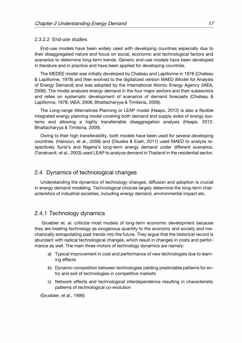
2.3.2.2 End-use studies
End-use models have been widely used with developing countries especially due to
their disaggregated nature and focus on social, economic and technological factors and
scenarios to determine long-term trends. Generic end-use models have been developed
in literature and in practice and have been applied for developing countries.
The MEDEE model was initially developed by Chateau and Lapillonne in 1978 (Chateau
& Lapillonne, 1978) and then evolved to the digitalized version MAED (Model for Analysis
of Energy Demand) and was adopted by the International Atomic Energy Agency (IAEA,
2006). The model analyses energy demand in the four major sectors and their subsectors
and relies on systematic development of scenarios of demand forecasts (Chateau &
Lapillonne, 1978; IAEA, 2006; Bhattacharyya & Timilsina, 2009).
The Long-range Alternatives Planning or LEAP model (Heaps, 2012) is also a flexible
integrated energy planning model covering both demand and supply sides of energy sys-
tems and allowing a highly transferrable disaggregation analysis (Heaps, 2012;
Bhattacharyya & Timilsina, 2009).
Owing to their high transferability, both models have been used for several developing
countries. (Hainoun, et al., 2006) and (Osueke & Ezeh, 2011) used MAED to analyze re-
spectively Syria’s and Nigeria’s long-term energy demand under different scenarios.
(Tanatvanit, et al., 2003) used LEAP to analyze demand in Thailand in the residential sector.
2.4 Dynamics of technological changes
Understanding the dynamics of technology changes, diffusion and adoption is crucial
in energy demand modeling. Technological choices largely determine the long-term char-
acteristics of industrial societies, including energy demand, environmental impact etc.
2.4.1 Technology dynamics
Gruebler et. al. criticize most models of long-term economic development because
they are treating technology as exogenous quantity to the economy and society and me-
chanically extrapolating past trends into the future. They argue that the historical record is
abundant with radical technological changes, which result in changes in costs and perfor-
mance as well. The main three motors of technology dynamics are namely:
a) Typical improvement in cost and performance of new technologies due to learn-
ing effects
b) Dynamic competition between technologies yielding predictable patterns for en-
try and exit of technologies in competitive markets
c) Network effects and technological interdependence resulting in characteristic
patterns of technological co-evolution
(Gruebler, et al., 1999)

18 2.4 Dynamics of technological changes
2.4.2 Technology diffusion and adoption
Since the pioneering work of (Mansfield, 1961) in terms of modeling the spreading of
new technologies, several mathematical forecasting models have been developed in liter-
ature: The Blackman model (Blackman, 1972), the Fisher-Pry model (Fisher & Pry, 1971),
the Gompertz curve (Martino, 1975), the Weibull model (Sharif & Islam, 1980) etc. These
models, also known as S-shaped curves, logistic substitution or diffusion curves are also
applicable for market diffusion (Bass, 1969; Gruebler, et al., 1999).
Figure 2: A simple case of technological substitution in the United States
(Gruebler, et al., 1999)
Figure 2 illustrates how motor cars replaced horse-drawn carriages in the United States.
Plotting the overall fraction of the number of units on the road shows clearly two symmet-
rical S-shaped curves.
Gruebler et. al. argue that the rate of diffusion of technologies is determined by many
factors, among other the four major ones are:
a) Relative advantage, comprising many dimensions including engineering (perfor-
mance, efficiency), economic (profitability, costs) and social (ease of adoption and
use)
b) Size, comprising many dimensions including geographical spread (local vs global),
market size (adoption in specialized application vs pervasive adoption)
c) Infrastructure needs (e.g. availability of electricity)
d) Interdependence with other technologies (network effects) i.e. the higher the inter-
dependence, the slower the individual technologies diffuse
(Gruebler, et al., 1999)
0
0.2
0.4
0.6
0.8
1
1900 1905 1910 1915 1920 1925 1930
Frac
tio
n F
(t)
Cars Horses
Chapter 2 Understanding Energy Demand 19
2.4.3 Technology transfer and diffusion in the context of developing
countries
There is a close relationship between a country’s economic and technological level of
development (Fagerberg & Verspagen, 2002). Trade openness is important to increase
growth by lowering barriers to technology adoption, which is a key determinant of interna-
tional differences in per-capita income (Hoekman, et al., 2005; Parente & Prescott, 1994).
Trade contributes to international technology transfer by allowing local reverse engineering
and access to new machinery and equipment (Hoekman, et al., 2005). Moreover, technol-
ogy adoption in developing countries is often subject to adapting to local circumstances
and existing methods (Evenson & Westphal, 1995). It is therefore important to consider
these particularities of developing countries when analyzing technology diffusion into the
market.
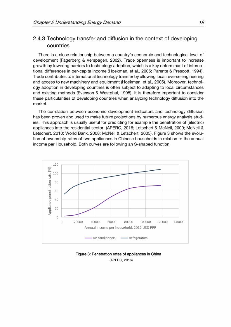
The correlation between economic development indicators and technology diffusion
has been proven and used to make future projections by numerous energy analysis stud-
ies. This approach is usually useful for predicting for example the penetration of (electric)
appliances into the residential sector: (APERC, 2016; Letschert & McNeil, 2009; McNeil &
Letschert, 2010; World Bank, 2008; McNeil & Letschert, 2005). Figure 3 shows the evolu-
tion of ownership rates of two appliances in Chinese households in relation to the annual
income per Household. Both curves are following an S-shaped function.
Figure 3: Penetration rates of appliances in China
(APERC, 2016)
0
20
40
60
80
100
120
0 20000 40000 60000 80000 100000 120000 140000
Ap
plia
nce
pen
etra
tio
n r
ate
[%]
Annual income per household, 2012 USD PPP
Air conditioners Refrigerators

20 2.5 Structure of electricity supply
It is important to note that in the following, energy is considered as the final energy
delivered to the end-user. This study also focuses only on electricity as final energy.
2.5 Structure of electricity supply
Electricity demand forecasting and peak load projection play an important role in
integrated resource planning and is key to formulating strategies and recommending
energy policies. In terms of supply safety, an underestimate could lead to under-capacity,
which results in a poor quality of service and even blackouts. Whereas an overestimate
could to lead to superfluous authorisation of costly plants. Projections also help quantify
the needed resources and assess different scenarios based on the variation of certain
variables (technical efficiency, demographic or economic growth etc.). (Swisher, et al.,
1997; Bhattacharyya & Timilsina, 2010; Mehra & Bharadwaj, 2000)
2.5.1 Load-duration curve
As a general assumption and as suggested by (Chen, et al., 2001), the electricity load
can be written as a function of four components:
𝐿 = 𝐿𝑛 + 𝐿𝑤 + 𝐿𝑠 + 𝐿𝑟
Where:
𝐿 : the total load
𝐿𝑛 : normal part of the load which is a set of standardized load shapes for each type of day
𝐿𝑤 : weather sensitive part of the load
𝐿𝑠 : special event part which is the occurrence of an unusual event leading to a significant
deviation from the typical behavior
𝐿𝑟 : random part which is an unexplained component usually represented as zero mean
white noise
(Chen, et al., 2001)
Based on this assumption, electric demand varies considerably during the course of the
day and the year. There are usually few hours of peak demand in a day for example when
residential and commercial demand overlap in late-afternoon, and several hours of low
demand during the night when activity is at its minimum. Moreover, there are seasons
where electricity demand is at higher demand for example during summer season due to
the higher air-conditioning demand.
Representing the specific demand during the day hours yields the demand load curve
which is an important input parameter for utilities to plan the generation dispatch. Figure 4
shows an example of a sample day load curve. One notices that the peak load occurs at
7 pm.

Chapter 2 Understanding Energy Demand 21
Figure 4: Sample system load curve for a Brazilian utility
(Swisher, et al., 1997)
The cumulative frequency distribution of load level during the year yields the load-du-
ration curve (Figure 5). The load-duration curve sorts the total hours of the year by de-
creasing demand. It usually shows the relative fraction of hours at the respective load level
(peak, intermediate or base load).
Figure 5: Sample load-duration curve
(Swisher, et al., 1997)
0
500
1000
1500
2000
2500
3000
3500
1 2 3 4 5 6 7 8 9 10 11 12 13 14 15 16 17 18 19 20 21 22 23 24
Dem
and
[M
W]
Hour
0
2000
4000
6000
8000
10000
12000
0% 10% 20% 30% 40% 50% 60% 70% 80% 90% 100%
Ho
url
y el
ectr
icit
y d
eman
d [
MW
]
Percentage of total hours in year [%]
peak load
intermediate load
base load
22 2.5 Structure of electricity supply
2.5.2 Load-curve projections
Projections of electricity demand are typically done for electricity on an annual basis in
terms of energy quantity (kWh). However, since it can be expensive to store electricity in
most of the cases, there must be a precise match between power production and the
hourly demand profile. The knowledge about the annual peak demand is also very im-
portant for utilities to plan the total capacity required in order to avoid power outages. It is
therefore crucial to project the future load profile to reflect the hourly, daily and seasonal
power fluctuations.
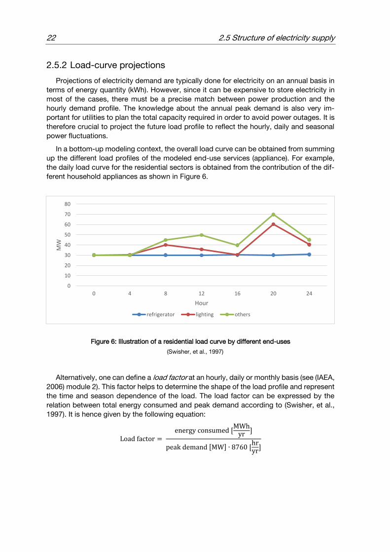
In a bottom-up modeling context, the overall load curve can be obtained from summing
up the different load profiles of the modeled end-use services (appliance). For example,
the daily load curve for the residential sectors is obtained from the contribution of the dif-
ferent household appliances as shown in Figure 6.
Figure 6: Illustration of a residential load curve by different end-uses
(Swisher, et al., 1997)
Alternatively, one can define a load factor at an hourly, daily or monthly basis (see (IAEA,
2006) module 2). This factor helps to determine the shape of the load profile and represent
the time and season dependence of the load. The load factor can be expressed by the
relation between total energy consumed and peak demand according to (Swisher, et al.,
1997). It is hence given by the following equation:
Load factor = energy consumed [
MWhyr
]
peak demand [MW] ∙ 8760 [hryr
]
0
10
20
30
40
50
60
70
80
0 4 8 12 16 20 24
MW
Hour
refrigerator lighting others
Chapter 3 An overview of ASEAN 23
3 An overview of ASEAN
The Association of Southeast Asian Nations (ASEAN) is a multi-faceted regional organ-
ization (Masilmani & Peterson, 2014) which comprises ten member states: Indonesia, Ma-
laysia, Philippines, Singapore, Thailand, Brunei Darussalam, Vietnam, Lao PDR, Myanmar
and Cambodia. As set out in the ASEAN Declaration (ASEAN, 1967) upon its foundation in
1967, its primary mandate is to establish greater economic, political, and cultural contact
and cooperation among its member states. The five founding members (Indonesia, Malay-
sia, Philippines, Singapore and Thailand) believed that, like many other inter-national or-
ganizations, structural integration would enhance political and security cooperation
(ASEAN, 2016; ADB, 2014). Over time, upon the transition of the region from conflict to
cooperation, the economy is taking center stage within ASEAN (ADB, 2014). In 2015, the
association established the ASEAN Economic Community (AEC) as a major milestone in
the regional economic integration agenda, offering a market of 2.6 trillion USD and over
622 million people (ASEAN, 2015).
This chapter comprises a short overview of ASEAN’s member countries in terms of eco-
nomic development (section 3.1) as well as their energy landscape (section 3.2).
3.1 ASEAN’s economy
In his 2014 speech in Berlin1, the ADB Vice-President for Operations Stephen P. Groff
said (ADB, 2014):
“If ASEAN were one economy, it would be seventh largest in the world
with a combined gross domestic product of $2.4 trillion in 2013. It could
be fourth largest by 2050 if growth trends continue […] With over 600
million people, ASEAN's potential market is larger than the European Un-
ion or North America. Next to the People's Republic of China and India,
ASEAN has the world's third largest labor force that remains relatively
young”
With the center of global economic gravity shifting toward Asia, and within Asia shifting
towards the two giant economies of the People’s Republic of China and India, it is sug-
gested that “economic size” is a significant advantage in accelerating growth and fostering
development. The AEC is hence an important milestone for ASEAN to keep pace with the
growth of these two regional powers, as well as with Japan, the Republic of Korea, and
other economies in the region — through competition and cooperation (ADB, 2014).
1 Keynote speech by ADB Vice-President for Operations 2 Stephen Groff at the "German-Business
Association AEC: Integration, Connectivity and Financing: What Does Regional Integration in South-
east Asia Mean for the German Business Community?" held on 23 June 2014 in Berlin, Federal
Republic of Germany
24 3.1 ASEAN’s economy
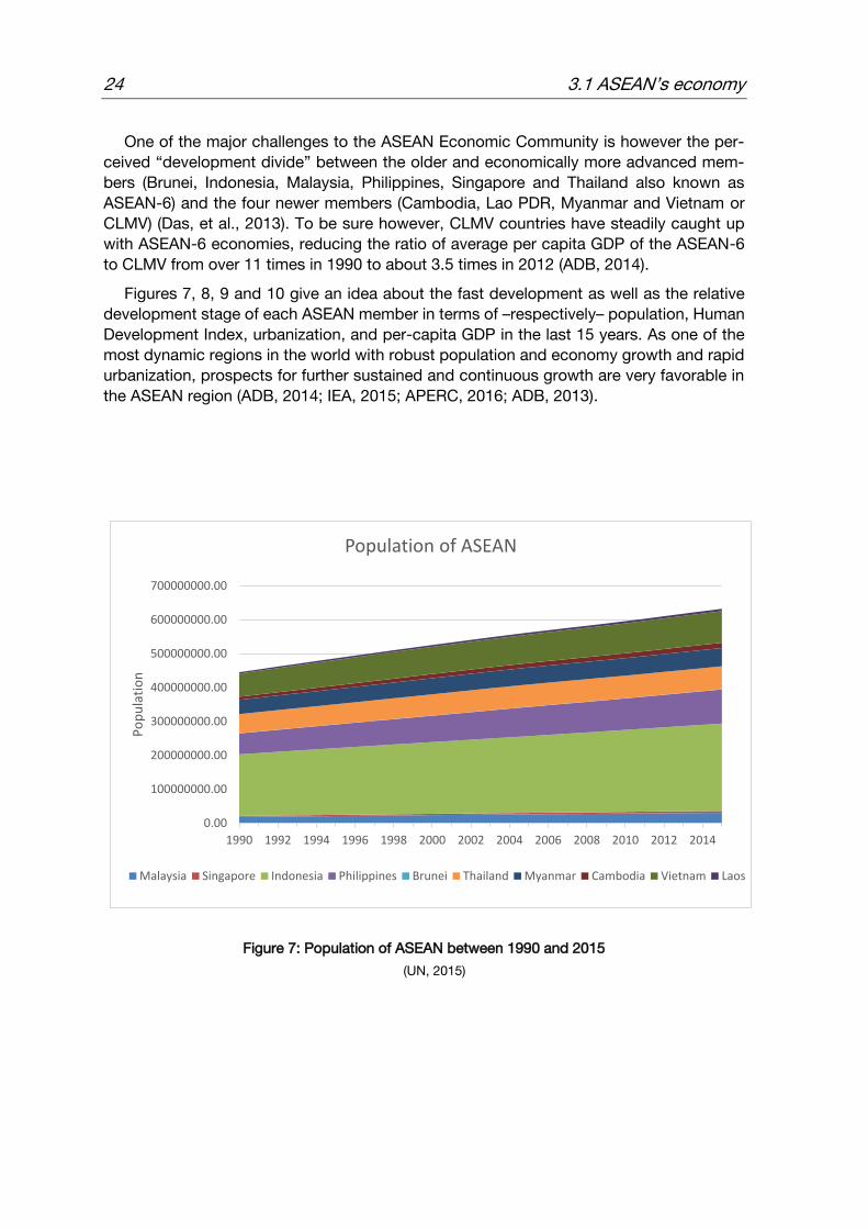
One of the major challenges to the ASEAN Economic Community is however the per-
ceived “development divide” between the older and economically more advanced mem-
bers (Brunei, Indonesia, Malaysia, Philippines, Singapore and Thailand also known as
ASEAN-6) and the four newer members (Cambodia, Lao PDR, Myanmar and Vietnam or
CLMV) (Das, et al., 2013). To be sure however, CLMV countries have steadily caught up
with ASEAN-6 economies, reducing the ratio of average per capita GDP of the ASEAN-6
to CLMV from over 11 times in 1990 to about 3.5 times in 2012 (ADB, 2014).
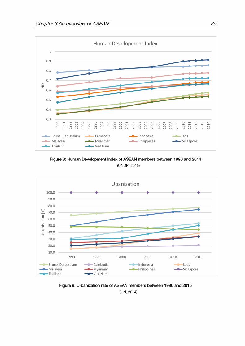
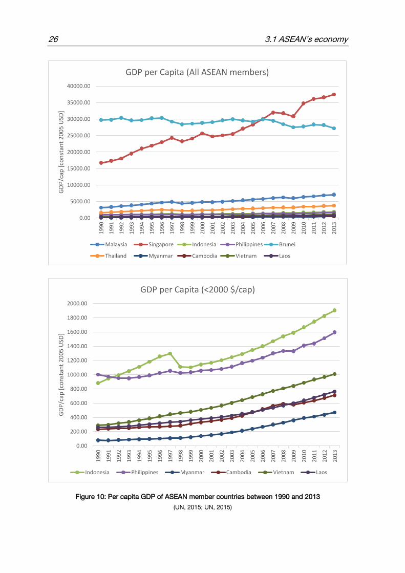
Figures 7, 8, 9 and 10 give an idea about the fast development as well as the relative
development stage of each ASEAN member in terms of –respectively– population, Human
Development Index, urbanization, and per-capita GDP in the last 15 years. As one of the
most dynamic regions in the world with robust population and economy growth and rapid
urbanization, prospects for further sustained and continuous growth are very favorable in
the ASEAN region (ADB, 2014; IEA, 2015; APERC, 2016; ADB, 2013).
Figure 7: Population of ASEAN between 1990 and 2015
(UN, 2015)
0.00
100000000.00
200000000.00
300000000.00
400000000.00
500000000.00
600000000.00
700000000.00
1990 1992 1994 1996 1998 2000 2002 2004 2006 2008 2010 2012 2014
Po
pu
lati
on
Population of ASEAN
Malaysia Singapore Indonesia Philippines Brunei Thailand Myanmar Cambodia Vietnam Laos
Chapter 3 An overview of ASEAN 25
Figure 8: Human Development Index of ASEAN members between 1990 and 2014
(UNDP, 2015)
Figure 9: Urbanization rate of ASEAN members between 1990 and 2015
(UN, 2014)
0.3
0.4
0.5
0.6
0.7
0.8
0.9
1
19
90
19
91
19
92
19
93
19
94
19
95
19
96
19
97
19
98
19
99
20
00
20
01
20
02
20
03
20
04
20
05
20
06
20
07
20
08
20
09
20
10
20
11
20
12
20
13
20
14
HD
IHuman Development Index
Brunei Darussalam Cambodia Indonesia Laos
Malaysia Myanmar Philippines Singapore
Thailand Viet Nam
10.0
20.0
30.0
40.0
50.0
60.0
70.0
80.0
90.0
100.0
1990 1995 2000 2005 2010 2015
Urb
anis
atio
n [
%]
Ubanization
Brunei Darussalam Cambodia Indonesia LaosMalaysia Myanmar Philippines SingaporeThailand Viet Nam
26 3.1 ASEAN’s economy
Figure 10: Per capita GDP of ASEAN member countries between 1990 and 2013
(UN, 2015; UN, 2015)
0.00
5000.00
10000.00
15000.00
20000.00
25000.00
30000.00
35000.00
40000.00
19
90
19
91
19
92
19
93
19
94
19
95
19
96
19
97
19
98
19
99
20
00
20
01
20
02
20
03
20
04
20
05
20
06
20
07
20
08
20
09
20
10
20
11
20
12
20
13
GD
P/c
ap [
con
stan
t 2
00
5 U
SD]
GDP per Capita (All ASEAN members)
Malaysia Singapore Indonesia Philippines Brunei
Thailand Myanmar Cambodia Vietnam Laos
0.00
200.00
400.00
600.00
800.00
1000.00
1200.00
1400.00
1600.00
1800.00
2000.00
19
90
19
91
19
92
19
93
19
94
19
95
19
96
19
97
19
98
19
99
20
00
20
01
20
02
20
03
20
04
20
05
20
06
20
07
20
08
20
09
20
10
20
11
20
12
20
13
GD
P/c
ap [
con
stan
t 2
00
5 U
SD]
GDP per Capita (<2000 $/cap)
Indonesia Philippines Myanmar Cambodia Vietnam Laos

Chapter 3 An overview of ASEAN 27
3.2 ASEAN’s energy landscape
3.2.1 Primary energy
The economic development of the ASEAN countries has induced a tremendous growth
of energy demand in the last decades (Huber, et al., 2015). The primary energy demand
has risen by more than 50% from 386 Mtoe in 2000 to 594 Mtoe in 2013. Fossil fuels
dominate the mix with the largest share for oil (Figure 11). This growing need for energy
has raised several challenges for the Southeast Asian countries: need for energy import
and concerns about energy security, increased exposure to volatile international fossil-fuel
prices, increase of pollution due to energy production and increase of the share of global
greenhouse-gas (GHG) emissions (IEA, 2015).
The region also has large differences in the primary energy mix between the countries
and the resources are not evenly distributed. While some countries like Indonesia, Malaysia
and Brunei, for example, have large fossil-fuel resources, other countries, however, are
relatively poor in indigenous fossil energy resources and rely mainly on energy imports
(IEA, 2015). Figure 12 presents an overview of the primary energy characteristics of each
ASEAN member.
Figure 11: Fuel shares in primary energy demand in ASEAN, 2000 and 2013
(ADB, 2013)
8%
41%
19%1%
26%
5%
2000: 386 MtoeCoal
Oil
Gas
Hydro
Bioenergy
Other renewables*
15%
36%22%
2%
21%
4%
2013: 594 Mtoe
*Includes solar PV, wind, and geothermal

28 3.2 ASEAN’s energy landscape
Figure 12: Primary energy overview of ASEAN countries
(IEA, 2015)
3.2.2 Power sector
The growth in energy demand and the increase of wealth and urbanization will lead to
an increased share of electricity in the final energy demand, and this trend might even be
accelerated by global warming (Morna & van Vuuren, 2009). Electricity is expected to ac-
count for more than 50% of future growth in energy demand, especially in the buildings
(residential and services) and industry sectors (IEA, 2015). All those aspects emphasize the
importance of the development of a sustainable, economic viable, environmental friendly,
and secure electricity supply (Huber, et al., 2015).

Chapter 3 An overview of ASEAN 29
Figure 13: Generation mix of the ASEAN countries in 2013
(IEA, 2016; UNSD, 2016)
As Figure 13 shows, power generation in ASEAN relies mostly on fossil fuels (coal, oil
and gas) and hydro power. Other regenerative sources play a minor role so far.
3.2.3 Integration of renewables and trans-border electricity trade
The high reliance on fossil fuels in ASEAN leads to a high level of CO2 emissions which
is increasing at a high pace. The regions energy related CO2 emissions are expected to rise
from less than 1.2 Gt of CO2 in 2013 to almost 2.4 Gt in 2040. This will result in doubling
the share of global emissions which amounts to 4% in 2013 (IEA, 2015). In the New Policies Scenario developed by the IEA, CO2 emissions grow at a faster pace than primary energy
demand due to the increasing share of coal in the energy mix (IEA, 2015). However, South-
east Asia is highly vulnerable to climate change as most of the people and of the economic
activities are located along the coastlines. A more frequent extreme weather also consti-
tutes a challenge for agricultural production. In order to reduce the risks lied to climate
change and to contribute to limiting global emissions, a transformation of ASEAN’s power
system towards a more sustainable system including higher shares of low-carbon energy
sources is inevitable (IEA, 2015; Huber, et al., 2015).
The Southeast Asian region offers abundant sources of renewable energies, which are
not anywhere utilized near to their potential. The reasons for that are mainly institutional
and political due to the concerns about the economic viability (Lidula, et al., 2007). More-
over, the renewable energy sources are unevenly distributed across the ASEAN region and
are mostly distant from the load centers in the megacities like Singapore or Bangkok (WEC,
2010; Lidula, et al., 2007). Trans-border electricity trade and the development of a common
ASEAN power grid offer the opportunity to maximize the benefit from integrating renewable
0%10%20%30%40%50%60%70%80%90%
100%
Generation mix in 2013
Coal Oil Gas Biofuel Waste Hydro Other renewables* Import
*Includes solar PV, wind, and geothermal
30 3.2 ASEAN’s energy landscape
energies and reduce total exploitation costs. Finding economically viable and technically
efficient pathways to achieve a transformation to such low-carbon power system is a main
challenge which has been tackled by some researchers: (Chang & Li, 2012; Kutani & Li,
2014; Huber, et al., 2015; Stich & Massier, 2015). Besides the optimization of the power
system as such, two important inputs of the system or model are the energy supply (and
in this case renewable energy potential) and energy demand.
3.2.4 Power demand and projection in ASEAN: existing research
There are several reports and studies dealing with the future ASEAN energy (and power)
demand like the APEC Energy Demand and Supply Outlook (APERC, 2016), the Southeast
Asia Energy Outlook (IEA, 2015), the ADB Energy Outlook for Asia and the Pacific (ADB,
2013), and the ASEAN Energy Outlook (ASEAN, 2015). Those studies in general consider
the whole energy supply system at an aggregated level and deliver projections based on
econometric methods and considerations. Power system optimization studies like (Huber,
et al., 2015) and (Chang & Li, 2012) are based on similar reports or methods to predict
ASEAN’s power demand in the next decades.
However, to get a technical and cost-related (including emission costs) optimization
which includes the fluctuations from renewable energy sources, it is necessary to input the
time dependent power demand i.e. the power load profiles. This is mainly due to the fact
that the development of power resources is rather dictated by the power demand during
peak times rather than by the annual power demand (Kutani & Li, 2014).
It is important to consider that load curves change due to changes in industrial structure
and living environment, which explains the load curve changes in many South East Asian
regions. In the mid-1990s, power consumption patterns in Thailand, the Philippines, Indo-
nesia (Java-Bali Transmission Line) and Vietnam (southern region) started to display load
curves which have a peak during daytime, which means that industrial and service related
demand is high due to the relatively mature market in these regions. Meanwhile, the power
consumption patterns in other less developed South East Asian regions like Laos and
Cambodia still have, until recent years, the traditional power load curve, where the daily
peak occurs from early evening due to lighting and residential load. However, with the
increasing power demand for industrial purposes due to economic development, the daily
peak is generally shifting more to the industry/service centered midday pattern (Kutani &
Li, 2014). Figure 14 shows the difference in patterns of a traditional household driven
evening peak (Laos) and an industry driven midday peak (Singapore).
Considering the dynamics which govern the daily load curve of a country, it is a chal-
lenging task to predict with accuracy future demand because they are intricately con-
nected to factors like culture, climate and economic circumstances. In studies like (Kutani
& Li, 2014) and (Stich & Massier, 2015), the general approach is to take actual load curves
from existing data (or from neighboring similar regions if the data is not available) and to
scale them according to the overall power consumption development in the future. The
problem of such an approach is that, as explained in the previous paragraph, it does not
consider structural changes in the economy as well as technological (e.g. increase of effi-
ciency) and social (e.g. urbanization) changes. The aim of this study is to solve this prob-
lem.

Chapter 3 An overview of ASEAN 31
Figure 14: Comparative normalized load profiles in a typical day of Singapore and Laos Data from (EMA, 2016) and (EDL, 2015)
0
0.00002
0.00004
0.00006
0.00008
0.0001
0.00012
0.00014
0.00016
0.00018
1 2 3 4 5 6 7 8 9 10 11 12 13 14 15 16 17 18 19 20 21 22 23 24
Normalised load profile
Singapore Laos

32 3.2 ASEAN’s energy landscape
4 Methodology
To model and project the power demand in ASEAN region, a hybrid bottom-up/top-
down approach is developed in this work. The modeling method is chosen depending on
the economic sectors, which are classified based on the IEA electricity statistics (IEA, 2016)
to four major power consuming sectors:
Industry: including mining, manufacturing, utilities and construction
Service: including wholesale, retail trade, restaurants and hotels, transport, stor-
age, communication, and public services
Residential: urban and rural households
Other: including agriculture, forestry, fishing, and other non-specified activities
Due to the fact that ASEAN differs structurally in terms of economic development and ac-
tivities and hence in terms of power consumption – as discussed in the previous chapter
– the method chosen for modeling power consumption in industrial and services sectors
(as well as “other” activities) is the top-down modeling approach. Since the residential
sector is the most homogeneous and uniform sector between these countries, it is mod-
eled in a bottom-up approach. Figure 15 depicts the overall structure of the model with the
respective inputs and outputs.
Figure 15: Global schema of the developed power demand projection model

Chapter 4 Methodology 33
This chapter goes through all the details of the model developed in this study, depicts
structure and assumptions of each of the top-down (section 4.2) and the bottom-up (sec-
tion 4.1) modeling, and explains the forecasting method as well as the developed scenarios
(4.3) in addition to the limits modeling approaches (4.4). Section 4.5 summarizes the
sources of the used data for modeling, and section 4.6 presents briefly the developed
tools.
4.1 Bottom-up modeling
4.1.1 Concept and structure
The end-use approach (bottom-up) is used, as explained above, for household power
consumption modeling. Initially the bottom-up model was based on the IAEA’s MAED
model structure (IAEA, 2006), then has been further developed to its actual form. As shown
in Figure 16, the model requires three major groups of inputs: socio-economic data, sta-
tistical data and meteorological data. The outputs of the model are: the annual electricity
consumption in the residential sector and its projection until 2040, and the corresponding
hourly load profiles for 8760 hours in each year.
Figure 16: Black-box structure of the end-use model for residential power demand

34 4.1 Bottom-up modeling
The inner structure of the model is based on accumulating the consumption of all ele-
ments which are divided into two categories: rural and urban households. The annual elec-
tricity consumption 𝑊annual consumption is hence expressed as:
𝑊annual consumption = 𝑊urban + 𝑊rural
The power consumption in each element (household) is obtained from the sum of the
power consumption of the electric appliances in the household.
The total consumption in each category is hence calculated as:
𝑊j = 𝑁𝑗 ∑ 𝑝𝑖,𝑗 ∙ 𝑊household,i,j
𝑖
Where:
𝑗 = rural/urban
𝑖 ∶ appliance index
𝑁𝑗 ∶ number of households in category 𝑗
𝑊household,𝑖,𝑗: specific power consumption of appliance 𝑖 per household of
category 𝑗
𝑝𝑖,𝑗 : penetration rate of appliance 𝑖 into households of category 𝑗
The total number of households 𝑁𝑗 is obtained from:
𝑁𝑗 = 𝑝𝑜𝑝 ∙ 𝜙𝑗
𝑠𝑗
Where:
𝑝𝑜𝑝 ∶ total population
𝜙𝑗 ∶ share of urban/rural population
𝑠𝑗 ∶ household size (number of inhabitants) in category 𝑗
The specific power consumption of an appliance is defined as follows:
𝑊household,i = ∑ 𝑛𝑖 ∙ ℎ𝑖 ∙ 𝑃𝑖365𝑡 (𝑡)
Where:
𝑃𝑖(𝑡) ∶ electric power of the appliance 𝑖, as function of the time of the year, in Watts
ℎ𝑖 ∶ the duration of use of appliance 𝑖 per day in hours
𝑛𝑖 ∶ quantity of appliances 𝑖 per household
The penetration rate of an appliance is defined as:
𝑝𝑖,𝑗 = 𝑂𝑤𝑖,𝑗 ∙ 𝐸𝑙𝑖,𝑗
Where:
𝑂𝑤𝑖,𝑗 ∶ ownership rate as the share of electrified households which own the appliance from
all electrified households
Equation 2
Equation 1
Chapter 4 Methodology 35
𝐸𝑙𝑖,𝑗 ∶ electrification rate as the share of electrified households from all the households in
the country
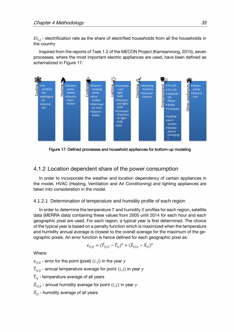
Inspired from the reports of Task 1.2 of the MECON Project (Kamsamrong, 2015), seven
processes, where the most important electric appliances are used, have been defined as
schematized in Figure 17.
Figure 17: Defined processes and household appliances for bottom-up modeling
4.1.2 Location dependent share of the power consumption
In order to incorporate the weather and location dependency of certain appliances in
the model, HVAC (Heating, Ventilation and Air Conditioning) and lighting appliances are
taken into consideration in the model.
4.1.2.1 Determination of temperature and humidity profile of each region
In order to determine the temperature 𝑇 and humidity 𝑋 profiles for each region, satellite
data (MERRA data) containing these values from 2005 until 2014 for each hour and each
geographic pixel are used. For each region, a typical year is first determined. The choice
of the typical year is based on a penalty function which is maximized when the temperature
and humidity annual average is closest to the overall average for the maximum of the ge-
ographic pixels. An error function is hence defined for each geographic pixel as:
𝑒𝑖𝑗,𝑦 = (�̅�𝑖𝑗,𝑦 − �̅�𝑖𝑗)2 + (�̅�𝑖𝑗,𝑦 − �̅�𝑖𝑗)2
Where:
𝑒𝑖𝑗,𝑦 ∶ error for the point (pixel) (𝑖, 𝑗) in the year 𝑦
�̅�𝑖𝑗,𝑦 ∶ annual temperature average for point (𝑖, 𝑗) in year 𝑦
�̅�𝑖𝑗 ∶ temperature average of all years
�̅�𝑖𝑗,𝑦 ∶ annual humidity average for point (𝑖, 𝑗) in year 𝑦
�̅�𝑖𝑗 ∶ humidity average of all years
Co
olin
g •Air-conditioner
•Refrigerator
•Electric fan
Hea
tin
g •Electric water heater
•Electric room heater
Co
oki
ng •Electric
cooking stove
•Rice cooker
•Microwave oven
•Electric Kettle
Ligh
tin
g •Incandes-cant light bulb
•Fluorescant light bulb
•Compact fluorescent light bulb
•LED
Cle
anin
g •Washing machine
•Vacuum cleaner
Ente
rtai
nm
ent •TV CRT
•TV LCD
•Video/DVD Player
•Radio
•Computer
•Laptop
•Hi-Fi system
•Mobile phone (charging)
Oth
er a
pp
lian
ces •Water
pump
•Electric iron
36 4.1 Bottom-up modeling
Then for each point (pixel) (𝑖, 𝑗), the years with the minimum and the maximum errors are
determined. The penalty function for each year is then calculated as the sum of the occur-
rences as year with minimum error minus the sum of the occurrences as year with maxi-
mum error. The year with the highest penalty function is chosen as the typical year.
Once the typical humidity and temperature profiles are obtained, a weighted geographic
average is calculated for the whole area. Since these profiles are used to determine elec-
tricity consumption in households, the weighing is hence based on the population density.
The final value for temperature/humidity is hence obtained from:
�̅� = 𝑇𝑖𝑗 ∙ 𝑤𝑖𝑗
Where:
�̅� ∶ final temperature profile for the selected region
𝑇𝑖𝑗 ∶ temperature profile at point (𝑖, 𝑗)
𝑤𝑖𝑗 ∶ normalized population density at point (𝑖, 𝑗)
4.1.2.2 Modeling of air-conditioners
Based on the approach developed in (Herzog & Hamacher, 2016), the following sub-
section aims to derive an expression of air-conditioner power demand as function of me-
teorological conditions.
The cooling process of an air-conditioner aims in one hand to cool down the exhaust
air and in the other hand to dehumidify it. The specific power 𝑃𝑒𝑙/�̇� of an air-conditioner
can be hence written as:
𝑃el
�̇�air=
∆ℎ1+𝑋
𝐶𝑂𝑃=
(ℎ(1+𝑋)O − ℎ(1+𝑋)C)
𝐶𝑂𝑃
Where:
∆ℎ1+𝑋 ∶ enthalpy difference between the humid air in the room (outside) and the cold ex-
haust air
ℎ(1+𝑋)O,C ∶ enthalpy of humid air (outside/cold)
𝐶𝑂𝑃 ∶ the coefficient of performance
Hence the air enters the air-conditioner from the outside (state O), and leaves is colder and
dehumidified (state C). The enthalpy of the humid air can be written as (Lucas, 2006):
ℎ(1+𝑋) = 𝑐air ∙ 𝑇 + 𝑋 ∙ (∆ℎ𝑉 + 𝑐vapor ∙ 𝑇)
Where:
𝑋 ∶ the absolute humidity of humid air
𝑇 ∶ the temperature
𝑐air, 𝑐vapor ∶ heat coefficients of respectively air and vapor
∆ℎ𝑉 ∶ the evaporation enthalpy at temperature 𝑇
The absolute humidity 𝑋 can be obtained from (Lucas, 2006):
Chapter 4 Methodology 37
𝑋 = 𝑀w
𝑀air∙
𝑝sw(𝑇)𝑝O𝜑
− 𝑝sw(𝑇)
Where:
𝑀w/air ∶ the molar mass of water/air
𝑝sw(𝑇) ∶ saturated vapor pressure at temperature 𝑇
𝑝O ∶ outside pressure
𝜑 ∶ relative humidity
The coefficient of performance is expressed as (Schmidt, et al., 2010):
𝐶𝑂𝑃 = 𝜂G ∙ 𝐶𝑂𝑃C = 𝜂G ∙𝑇ev
𝑇co − Tev
Where:
𝐶𝑂𝑃C ∶ Carnot ideal COP
𝜂G ∶ inner efficiency of the machine, typical values are 0.4 … 0.6 (Wyssen, et al., 2010)
𝑇ev ∶ Temperature at the evaporator of the chiller
𝑇co ∶ Temperature at the condenser of the chiller
The evaporator temperature 𝑇ev depends on the target cooling temperature. This latter
target state 𝐶 can be assumed based on (DIN EN 15251, 2007) as:
𝑇𝐶 = 22°; 𝜑𝐶 = 50% → 𝑋𝐶 = 0.0083 kg water
kg dry air
To dehumidify the ambient air, a cooling to the dew point 𝑇τ(𝑇C, 𝜑C) = 11.1 ℃ is necessary.
The temperature difference in the evaporator and in the condenser is assumed to be
around 10 K (Herzog & Hamacher, 2016). The COP is hence expressed as function of the
outside temperature 𝑇O and the target cooling 𝑇C temperature as:
𝐶𝑂𝑃 = 𝜂G ∙𝑇τ(𝑇C, 𝜑C) − 10K
𝑇O + 10K − (𝑇τ(𝑇C, 𝜑C) − 10K)
Finally, the air-conditioner power can be written as a function of the ambient air condition
(Temperature and humidity) and the operating parameters of the machine:
𝑃el
�̇�air=
𝑇A − 𝑇τ(𝑇C, 𝜑C) + 20K
𝜂G ∙ (𝑇τ(𝑇C, 𝜑C) − 10K)∙ (𝑐air(𝑇O − 𝑇C) + (𝑋O − 𝑋C) ∙ (∆ℎV + 𝑐vapor ∙ (𝑇O − 𝑇C)))
All used thermodynamics values and technical assumptions are listed in appendix A).
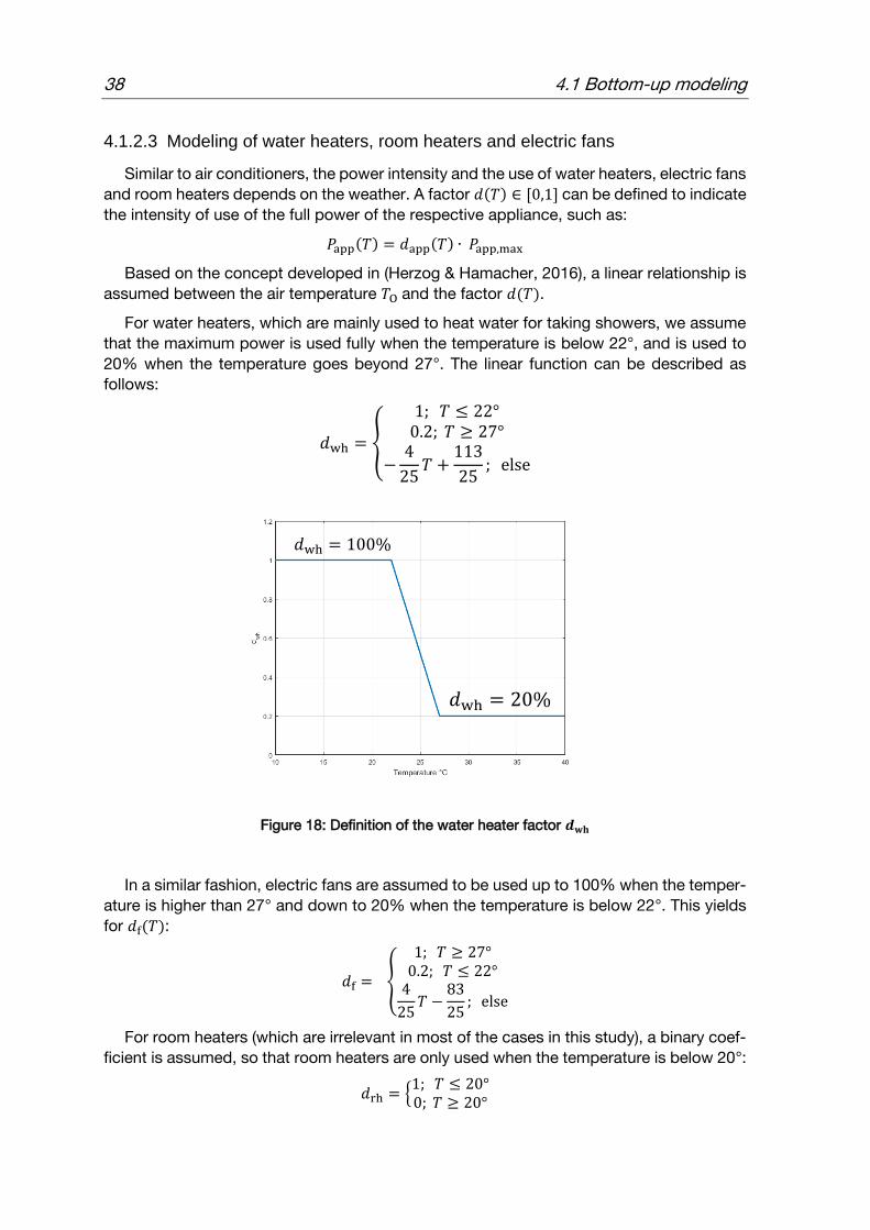
38 4.1 Bottom-up modeling
4.1.2.3 Modeling of water heaters, room heaters and electric fans
Similar to air conditioners, the power intensity and the use of water heaters, electric fans
and room heaters depends on the weather. A factor 𝑑(𝑇) ∈ [0,1] can be defined to indicate
the intensity of use of the full power of the respective appliance, such as:
𝑃app(𝑇) = 𝑑app(𝑇) ∙ 𝑃app,max
Based on the concept developed in (Herzog & Hamacher, 2016), a linear relationship is
assumed between the air temperature 𝑇O and the factor 𝑑(𝑇).
For water heaters, which are mainly used to heat water for taking showers, we assume
that the maximum power is used fully when the temperature is below 22°, and is used to
20% when the temperature goes beyond 27°. The linear function can be described as
follows:
𝑑wh = {
1; 𝑇 ≤ 22°0.2; 𝑇 ≥ 27°
−4
25𝑇 +
113
25; else
Figure 18: Definition of the water heater factor 𝒅𝐰𝐡
In a similar fashion, electric fans are assumed to be used up to 100% when the temper-
ature is higher than 27° and down to 20% when the temperature is below 22°. This yields
for 𝑑f(𝑇):
𝑑f = {
1; 𝑇 ≥ 27°0.2; 𝑇 ≤ 22°
4
25𝑇 −
83
25; else
For room heaters (which are irrelevant in most of the cases in this study), a binary coef-
ficient is assumed, so that room heaters are only used when the temperature is below 20°:
𝑑rh = {1; 𝑇 ≤ 20°0; 𝑇 ≥ 20°
𝑑wh = 100%
𝑑wh = 20%

Chapter 4 Methodology 39
4.1.2.4 Modeling lighting appliances
The use of lights in households also depends on sunset and sunrise time and is there-
fore a function of the location. The time of day at which the sun sets and rises can be
calculated for each region, given its geographic coordinates, using the sun angles.
To calculate the sunset/sunrise sun angle, one needs to determine the sun declination of
the year’s day (Page, 2003):
𝛿 = sin−1(0.3978) ∙ sin (𝐽′ − 1.4 + 0.0355 ∙ sin(𝐽′ − 0.0489))
Where:
𝐽′ ∶ the day angle in radians = Julian day number × 2𝜋/365.25
The sunset angle calculates then to (Page, 2003):
𝜔𝑠 = cos−1(−tan𝜙 tan𝛿)
Where:
𝜙 ∶ the latitude angle in radians
To convert values from the local apparent time LAT (solar time) to the local mean time LMT
(clock time), the Equation of Time EOT is needed (Page, 2003):
EOT = −0.128 sin(𝐽′ − 2.8°) = 0.165 sin(2𝐽′ + 19.7°) hours
The conversion yields:
LAT = LMT +(𝜆 − 𝜆𝑅)
15+ EOT − 𝑐 hours
Where:
𝜆 ∶ the longitude of the site in degrees
𝜆𝑅 ∶ the longitude of the time zone in which the site is situated (in degrees)
𝑐 ∶ summer time correction (if applicable)
Sunset and sunrise times are hence obtained from:
time = 12 ±𝜔𝑠
15−
(𝜆 − 𝜆𝑅)
15
4.1.3 Generating power load profiles
In order to obtain the hourly electric load, ℎ𝑖 from Equation 1 can be written as:
ℎ𝑖,𝑚 = ℎ𝑖,𝑚̅̅ ̅̅ ̅ ∑ 𝜌𝑖,𝑚,𝑙
24
𝑙=1
Where:
𝑚 = weekday, weekend
ℎ𝑖,𝑚̅̅ ̅̅ ̅ ∶ a constant duration of use of appliance 𝑖
𝜌𝑖,𝑚,𝑙 ∶ the probability of using appliance 𝑖 at the hour 𝑙 of the day, with ∑ 𝜌𝑖,𝑚,𝑙𝑙 = 1

40 4.1 Bottom-up modeling
We obtain therefore an hour coefficient ℎ𝑖,𝑚,𝑙 = ℎ𝑖,𝑚̅̅ ̅̅ ̅ ∙ 𝜌𝑖,𝑚,𝑙. The probability of use of an
appliance 𝜌𝑖,𝑚,𝑙 depends mainly on behavioral factors and best determined through meas-
urement data. There are also different behavioral characteristics of the usage of the appli-
ances during week-days and week-ends, and therefore the definition of two different prob-
ability functions. The probability distribution values used in this work are based on previous
studies: (Pratt, et al., 1989; Hendron & Engebrecht, 2010; Eto, et al., 1990; LaCommare, et
al., 2002).
Figure 19 shows the probability distribution function of the usage of air-conditioners as
an example. For lighting appliances, the probability of usage is adjusted to sunset and
sunrise timings - as calculated in the previous paragraph. All used probability distribution
functions are schematized in appendix B).
Figure 19: Usage probability distribution for air-conditioner
Load profiles from (LaCommare, et al., 2002; Pratt, et al., 1989)
4.1.4 Demand forecasting
In the context of bottom-up modeling, obtaining demand forecasts, which is the model
output, translates into injecting forecasts of the input variables into the model. To obtain
those forecasts of the input variables, as described in 4.1.1, several methods are used in
this study, depending on the input variable.
Table 1 sums up the methods used to forecast each of the input variables. Part of the
input forecasts (for population, urbanization, and GDP) are obtained from external sources.
Forecasts for household size and electrification rate/appliance ownership rate are obtained
through methods explained further in this subsection.
0.00
0.01
0.02
0.03
0.04
0.05
0.06
0.07
0.08
0.09
1 2 3 4 5 6 7 8 9 10 11 12 13 14 15 16 17 18 19 20 21 22 23 24
𝜌
hour
Usage probability distribution for air-conditioner
week-day
week-end

Chapter 4 Methodology 41
Input variables Projection method
Population, urbanization External source: UN data bank (see 4.5)
GDP growth External source: Different studies (see 4.5)
Technical efficiency Assumption depending on scenario: linear improvement
Household size UN method: based on past trend and pop-ulation data
Electrification rate/appliance ownership rate
Correlation with GDP per capita
Table 1: Used methods for input variables projection (bottom-up modeling)
4.1.4.1 Technical efficiency
The electric power of the appliance 𝑃𝑖 is assumed constant unless it depends on the
meteorological data. Since the technical efficiency of electrical appliances is likely to im-
prove with the adoption of new technologies, this variable can be included in the future
projections. For this work a linear improvement is assumed, and its magnitude depends
on the chosen scenario.
4.1.4.2 Household size projection
In many countries, and especially developing countries, the number of households
grows at a considerably different rate from that of total population (due to urbanization and
nuclearization of the family) (UN, 1973). It is therefore important to consider projections for
household size in order to obtain the total number of households in the future.
The method followed in this study is a UN method for households’ projection which is
further explained in (UN, 1973) (Methods not using headship rate). This method relies on
defining the ratio between the number of households and the adult population (between
15 to 64 years old (World Bank, 2008)) since household formation is confined to this section
of the population. This ratio ℎ𝑡 is a function of time (year) and can be projected based on
historical data according to the following formula (UN, 1973):
ℎ𝑡 = 1 − (1 − ℎ𝑡1) (1 − ℎ𝑡2
1 − ℎ𝑡1)
𝑡−𝑡1𝑡2−𝑡1
Knowing future trends for total population and for population by five-year age groups, the
total number of households and equivalently average household size can be projected as
well.

42 4.1 Bottom-up modeling
4.1.4.3 Electrification rate and appliance ownership projection
As discussed in 2.4, technologies diffuse gradually into society in form of logistic func-
tions, and in the context of developing countries the national economic situation is the
main driver for this diffusion (Letschert & McNeil, 2009; World Bank, 2008). For this study,
a Weibull function (Sharif & Islam, 1980) is adopted to model the future penetration of ap-
pliances into households 𝑂𝑤𝑖,𝑗 as well as the electrification rates 𝐸𝑙𝑖,𝑗 (see Equation 2).
The Weibull cumulative distribution function (CDF) describes the shape of an S-function
regarding two parameters: a shape parameter 𝛽 and a scale parameter 𝛼 as shown in Fig-
ure 20.
𝑭(𝒙) = 𝟏 − 𝒆−(𝒙
𝜶)
𝜷
𝐟𝐨𝐫 𝒙 > 𝟎
Figure 20 Weibull CDF for different values of 𝜶 (𝜷 = 𝟑) and different values of 𝜷 (𝜶 = 𝟒)
(Sharif & Islam, 1980)
The parameters 𝛽 and 𝛼 are estimated through transforming Equation 3 to a linear re-
gression problem according to:
𝐹(𝑥) = 1 − 𝑒−(
𝑥𝛼
)𝛽
⟺ 𝑙𝑛 (𝑙𝑛1
1 − 𝐹(𝑥)) = 𝛽 𝑙𝑛(𝛼) + 𝛽 𝑙𝑛(𝑥)
⟺ 𝑌 = 𝐴 + 𝐵𝑋
With:
𝑌 = 𝑙𝑛 (𝑙𝑛1
1−𝐹(𝑥))
𝐴 = 𝛽 ln(𝛼)
𝐵 = 𝛽
𝑋 = ln(𝑥)
The correlation is established for each series (appliances ownership and electrification
rates for rural and urban areas) with the GDP/cap PPP in the x axis and the ownership rate
or the electrification rate in the y axis. The data used for the correlation is from different
countries in different development levels. Figure 20 and Figure 21 show three examples of
the resulted Weibull functions. All obtained data and correlations are represented in ap-
pendix C).
Equation 3
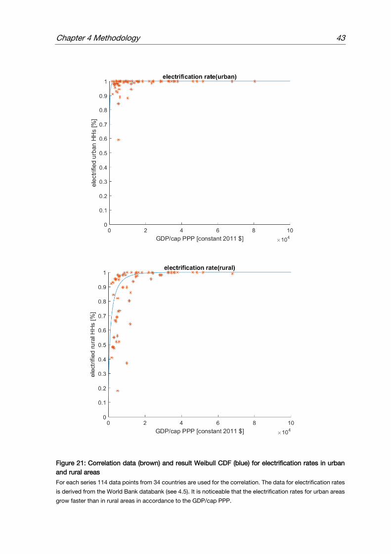
Chapter 4 Methodology 43
Figure 21: Correlation data (brown) and result Weibull CDF (blue) for electrification rates in urban
and rural areas
For each series 114 data points from 34 countries are used for the correlation. The data for electrification rates
is derived from the World Bank databank (see 4.5). It is noticeable that the electrification rates for urban areas
grow faster than in rural areas in accordance to the GDP/cap PPP.
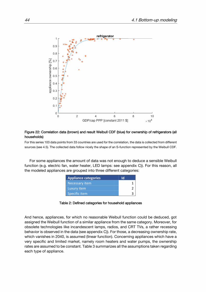
44 4.1 Bottom-up modeling
Figure 22: Correlation data (brown) and result Weibull CDF (blue) for ownership of refrigerators (all
households)
For this series 103 data points from 33 countries are used for the correlation, the data is collected from different
sources (see 4.5). The collected data follow nicely the shape of an S-function represented by the Weibull CDF.
For some appliances the amount of data was not enough to deduce a sensible Weibull
function (e.g. electric fan, water heater, LED lamps: see appendix C)). For this reason, all
the modeled appliances are grouped into three different categories:
Appliance categories Id
Necessary item 1
Luxury item 2
Specific item 3
Table 2: Defined categories for household appliances
And hence, appliances, for which no reasonable Weibull function could be deduced, got
assigned the Weibull function of a similar appliance from the same category. Moreover, for
obsolete technologies like incandescent lamps, radios, and CRT TVs, a rather recessing
behavior is observed in the data (see appendix C)). For those, a decreasing ownership rate,
which vanishes in 2040, is assumed (linear function). Concerning appliances which have a
very specific and limited market, namely room heaters and water pumps, the ownership
rates are assumed to be constant. Table 3 summarizes all the assumptions taken regarding
each type of appliance.

Chapter 4 Methodology 45
Appliances Category Remarks
Air-conditioner 1 ✓
Refrigerator 1 ✓
Electric fan 1 Refrigerator
Electric Kettle 2 Rice cooker
Electric water heater 1 Air-conditioner
Electric room heater 3 Constant ownership
Electric cooking stove 2 ✓
Rice cooker 2 ✓
Microwave oven 2 ✓
Incandescent light bulb 3 Recessing behavior
Fluorescent light bulb 1 ✓
Compact fluorescent light bulb 1 Fluorescent light bulb
LED 1 Fluorescent light bulb
Washing machine 1 ✓
Vacuum cleaner 2 ✓
TV CRT 3 Recessing behavior
TV LCD 1 ✓
Video/DVD Player 2 ✓
Radio 3 Recessing behavior
Computer 2 ✓
Laptop 2 ✓
Hi-Fi system 2 ✓
Mobile phone (charging) 1 ✓
Water pump 3 Constant ownership
Electric iron 1 Washing machine
Table 3: Assumptions regarding appliances ownership projection
The second column defines to which category the appliance belongs (see Table 2), the third column indicates
whether the Weibull function of another appliance is assigned (yellow), the ownership is assumed constant
(grey) or receding (orange)
The determined overall correlation prescribes a general trend in the development of the
respective variable (electrification/appliance ownership) in relation to economic growth. It
does not obviously predict the actual single data points, which are statistically distributed
around the curve. In order to adjust the prediction to each data point, two different adjust-
ment methods are suggested. The first method relies on adjusting the scale factor 𝛼 in
order for the curve to meet the considered data point (Figure 23). This method takes into
consideration the “delay” in development of the observed variable (ownership/electrifica-
tion rate) of each country, and results into “pulling” the curve to meet this delay. The sec-
ond method is to simply shift the curve horizontally in order to meet the considered data
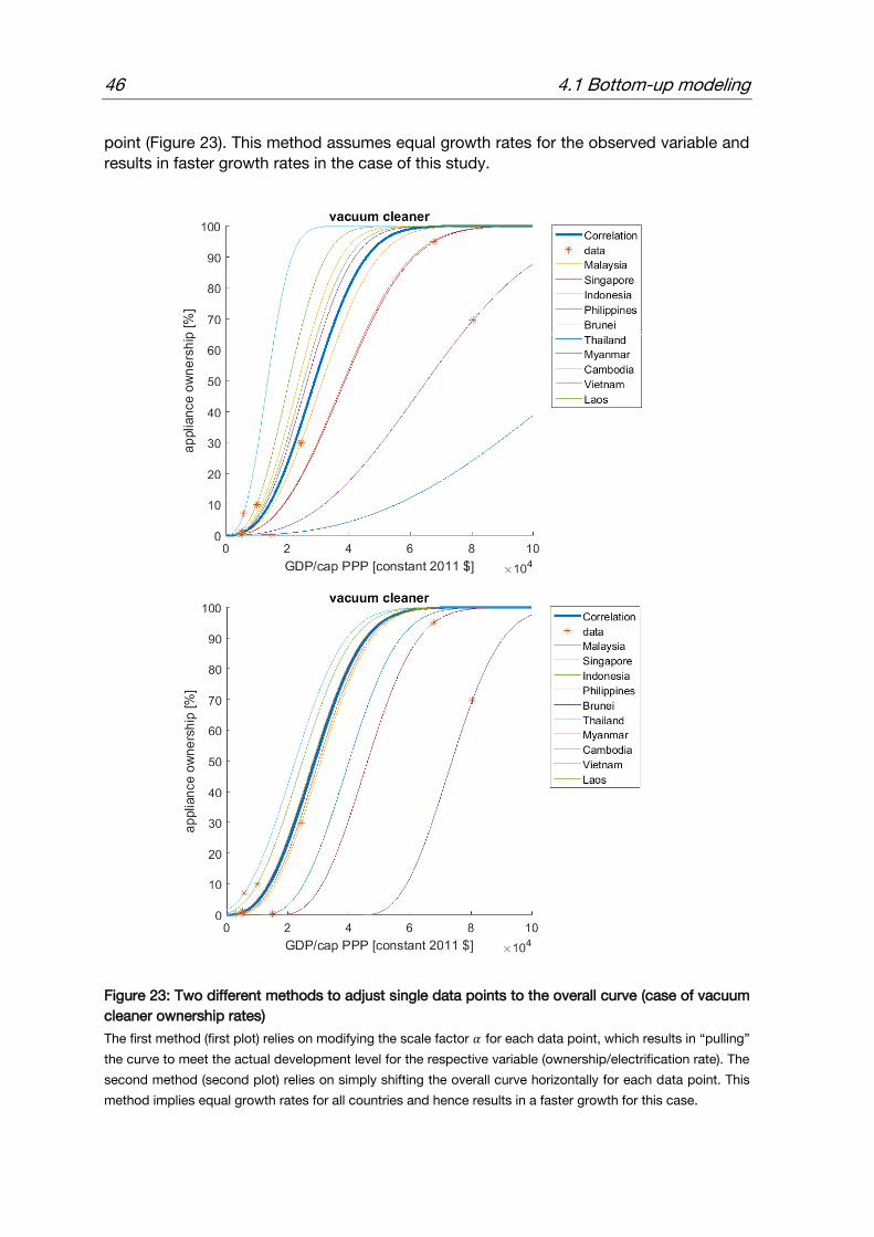
46 4.1 Bottom-up modeling
point (Figure 23). This method assumes equal growth rates for the observed variable and
results in faster growth rates in the case of this study.
Figure 23: Two different methods to adjust single data points to the overall curve (case of vacuum
cleaner ownership rates)
The first method (first plot) relies on modifying the scale factor 𝛼 for each data point, which results in “pulling”
the curve to meet the actual development level for the respective variable (ownership/electrification rate). The
second method (second plot) relies on simply shifting the overall curve horizontally for each data point. This
method implies equal growth rates for all countries and hence results in a faster growth for this case.
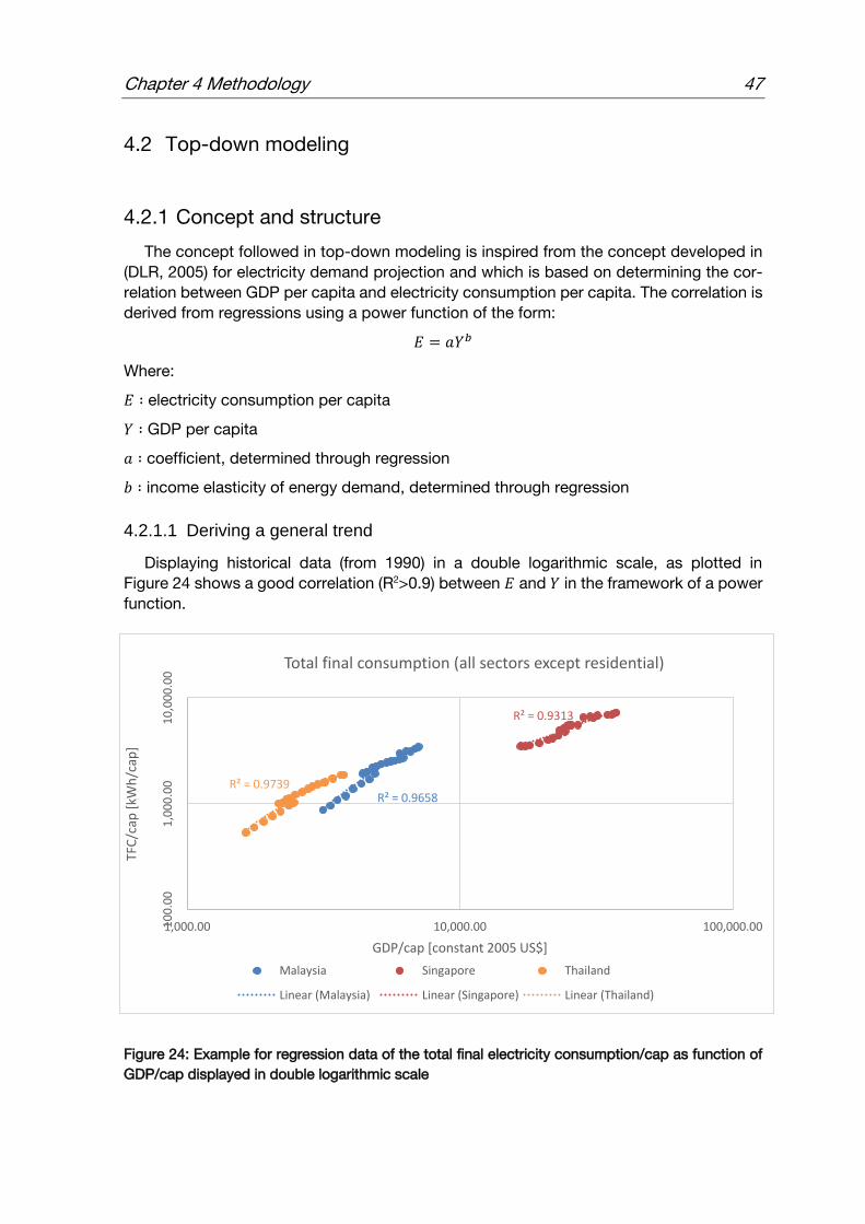
Chapter 4 Methodology 47
4.2 Top-down modeling
4.2.1 Concept and structure
The concept followed in top-down modeling is inspired from the concept developed in
(DLR, 2005) for electricity demand projection and which is based on determining the cor-
relation between GDP per capita and electricity consumption per capita. The correlation is
derived from regressions using a power function of the form:
𝐸 = 𝑎𝑌𝑏
Where:
𝐸 ∶ electricity consumption per capita
𝑌 ∶ GDP per capita
𝑎 ∶ coefficient, determined through regression
𝑏 ∶ income elasticity of energy demand, determined through regression
4.2.1.1 Deriving a general trend
Displaying historical data (from 1990) in a double logarithmic scale, as plotted in
Figure 24 shows a good correlation (R2>0.9) between 𝐸 and 𝑌 in the framework of a power
function.
Figure 24: Example for regression data of the total final electricity consumption/cap as function of
GDP/cap displayed in double logarithmic scale
R² = 0.9658
R² = 0.9313
R² = 0.9739
10
0.0
01
,00
0.0
01
0,0
00
.00
1,000.00 10,000.00 100,000.00
TFC
/cap
[kW
h/c
ap]
GDP/cap [constant 2005 US$]
Total final consumption (all sectors except residential)
Malaysia Singapore Thailand
Linear (Malaysia) Linear (Singapore) Linear (Thailand)

48 4.2 Top-down modeling
However, and as already discussed in 2.2.2, relying only on past experiences may be
misleading as technological, economic, political and social development may change de-
velopment patterns (DLR, 2005). In this context and using data from 37 countries over 13
years (481 data points), we can observe that the income elasticity 𝑏 is higher for less de-
veloped countries relative to a lower value for 𝑏 for more developed nations (compare for
example the slopes between Thailand and Singapore in Figure 24), which means that the
development rate of electricity consumption as function of GDP is high for developing
countries and slowly reaches a certain “saturation” level as the country is further devel-
oped. Departing from this observation, the assumption is made that, the overall growth
trend in electricity consumption would follow the same “path” from high growth rates at
lower GDP/cap to lower growth rates at higher GDP/cap. This translates to expressing
elasticity 𝑏 (and consequently coefficient 𝑎) as function of GDP/cap. Since 𝑏 and 𝑎 are
determined through regression (and cannot be calculated punctually), the idea is to define
intervals for GDP/cap values, and calculate respectively coefficients 𝑏 and 𝑎 in each inter-
val. Those GDP/cap intervals are mainly based on the level of development of the coun-
tries, hence the Human Development Index HDI is used as a reference to define three
development levels as shown in Table 4.
Development level HDI
High development HDI ≥ 0.8
Medium development 0.6 ≤ HDI < 0.8
Low development HDI < 0.6
Table 4: Country clustering definition according to Human Development Index HDI
Based on this clustering, and using data from 37 countries, three sets of parameters 𝑏𝑖
and 𝑎𝑖 (𝑖 = 1,2,3) are determined through least squares regression. To determine the GDP
intervals mentioned earlier, the intersection points of the regression lines in the double
logarithmic scale are chosen as boundaries of each interval as shown in Figure 25. We can
hence define the resulted elasticity function �̃�(𝑌) as:
�̃�(𝑌) = {
𝑏1 if 𝑌 < 𝑌1
𝑏2 if 𝑌1 < 𝑌 < 𝑌2
𝑏3 if 𝑌 > 𝑌2
Where
𝑌 ∶ GDP/capita
𝑌1,2 ∶ the intersection points of the regression results
The same procedure is applied separately for service, industry and the total consump-
tion (without including the residential sector). The resulting power functions are plotted in
Figure 26. More details about the regression procedure are represented in appendix D).

Chapter 4 Methodology 49
Figure 25: Correlation data for the industry sector, represented in double logarithmic scale
It is clearly visible in this plot that the slope of the regression line (i.e. the income elasticity) is decreasing with
increasing GDP/cap. The intersection between the regression results for each group of countries (cluster) de-
fines the borders of each GDP interval. The final power function is hence defined per interval.
0.00000000000
1.00000000000
2.00000000000
3.00000000000
4.00000000000
5.00000000000
6.00000000000
7.00000000000
8.00000000000
9.00000000000
10.00000000000
4.00 5.00 6.00 7.00 8.00 9.00 10.00 11.00 12.00
ln(F
inal
Co
nsu
mp
tio
n/c
ap)
ln(GDP/cap)
Industry fit: Industry 1 fit: Industry 2 fit: Industry 3
GDP interval 1 GDP interval 2 GDP interval 3
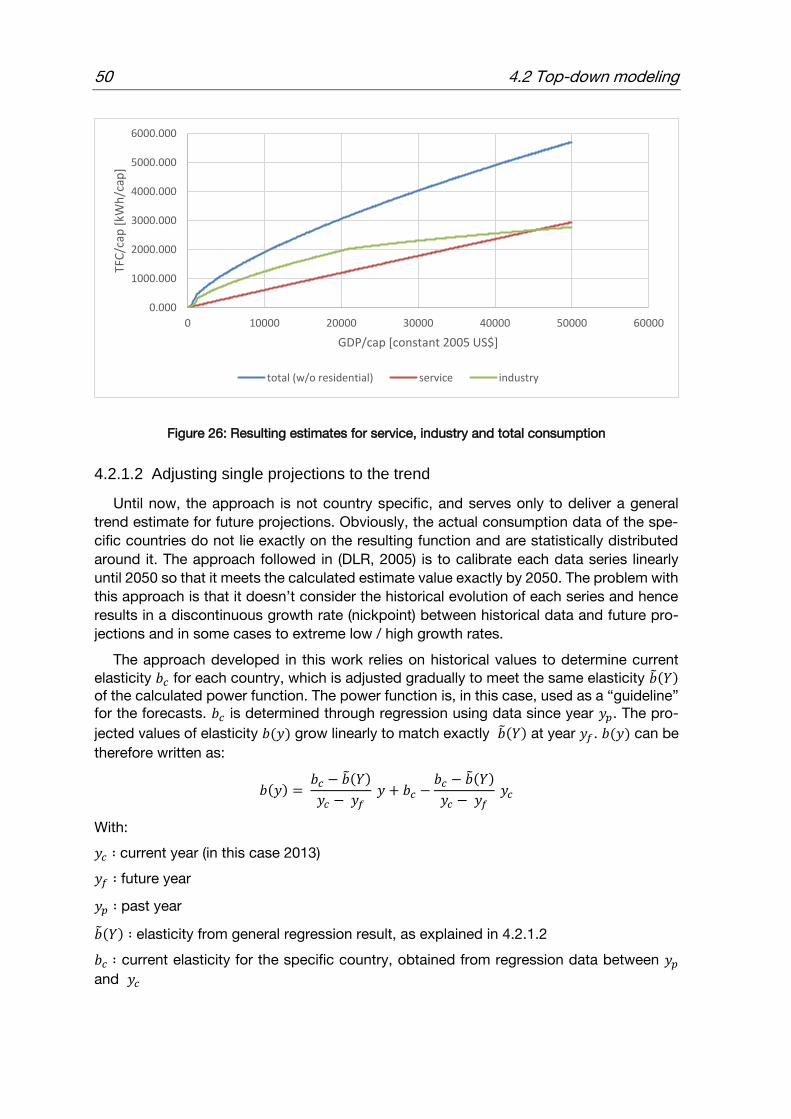
50 4.2 Top-down modeling
Figure 26: Resulting estimates for service, industry and total consumption
4.2.1.2 Adjusting single projections to the trend
Until now, the approach is not country specific, and serves only to deliver a general
trend estimate for future projections. Obviously, the actual consumption data of the spe-
cific countries do not lie exactly on the resulting function and are statistically distributed
around it. The approach followed in (DLR, 2005) is to calibrate each data series linearly
until 2050 so that it meets the calculated estimate value exactly by 2050. The problem with
this approach is that it doesn’t consider the historical evolution of each series and hence
results in a discontinuous growth rate (nickpoint) between historical data and future pro-
jections and in some cases to extreme low / high growth rates.
The approach developed in this work relies on historical values to determine current elasticity 𝑏𝑐 for each country, which is adjusted gradually to meet the same elasticity �̃�(𝑌) of the calculated power function. The power function is, in this case, used as a “guideline” for the forecasts. 𝑏𝑐 is determined through regression using data since year 𝑦𝑝. The pro-
jected values of elasticity 𝑏(𝑦) grow linearly to match exactly �̃�(𝑌) at year 𝑦𝑓. 𝑏(𝑦) can be
therefore written as:
𝑏(𝑦) = 𝑏𝑐 − �̃�(𝑌)
𝑦𝑐 − 𝑦𝑓 𝑦 + 𝑏𝑐 −
𝑏𝑐 − �̃�(𝑌)
𝑦𝑐 − 𝑦𝑓 𝑦𝑐
With:
𝑦𝑐 ∶ current year (in this case 2013)
𝑦𝑓 ∶ future year
𝑦𝑝 ∶ past year
�̃�(𝑌) ∶ elasticity from general regression result, as explained in 4.2.1.2
𝑏𝑐 ∶ current elasticity for the specific country, obtained from regression data between 𝑦𝑝
and 𝑦𝑐
0.000
1000.000
2000.000
3000.000
4000.000
5000.000
6000.000
0 10000 20000 30000 40000 50000 60000
TFC
/cap
[kW
h/c
ap]
GDP/cap [constant 2005 US$]
total (w/o residential) service industry

Chapter 4 Methodology 51
The values for 𝑦𝑝 and 𝑦𝑓 are determined empirically relying on comparing the final estimate
results of the model to estimates from other similar studies.
This procedure is applied separately for industry, service, and the total consumption
(w/o residential part). The final consumption for the “other” sector is obtained from sub-
tracting industry and service estimates from the total consumption estimate.
4.2.1.3 Technical efficiency
In a similar fashion to residential demand (4.1.4.1), a linear improvement of the efficiency
can be assumed for some scenarios. It can be applied as a factor to the final demand
result.
4.2.2 Deriving power load profiles
Contrary to bottom-up modeling, load profiles are derived top-down from the total es-timated electricity consumption 𝑊𝑗 ; (𝑗 = industry, service, other). To do so, three important
factors contribute to deriving the load profile:
Profile shape: defined as an hour coefficient ℎ𝑖 such as ∑ ℎ𝑖,𝑗24𝑖=1 = 24
The ratio of the week-day to week-end load: defined as two day coefficients 𝑑wd
and 𝑑we such as 5 𝑑wd + 2 𝑑we = 7
The share of load used for cooling end-uses: defined as a percentage 𝜙cooling,𝑗.
Accordingly, hour coefficients for cooling ℎcooling,𝑖 for the whole year are calcu-
lated based on the results from paragraph 4.1.2.2 such as ∑ ℎcooling,𝑖 = 87608760𝑖=1
The total load for hour 𝑖 in sector 𝑗 in a week-day, for example, sums up hence to:
𝐿𝑖,wd,j =𝑊𝑗
8760∙ 𝑑wd ∙ ℎ𝑖,𝑗 ∙ (𝜙cooling,𝑗 ∙ ℎcooling,𝑖 + (1 − 𝜙cooling,𝑗))
Several literature sources (Karali, et al., 2015; Jakob, et al., 2014; Ponniran, et al., 2012)
as well as the observation of actual load data (appendix F)) show a relatively uniform
shaped load profile for the sectors industry and service, which are mainly characterized
through a midday peak with a small drop during lunch break time. For this study constant
shapes for the load profiles are assumed as shown in Figure 27.

52 4.3 Projection scenarios
Figure 27: Load profile shapes (hour coefficients)
Load profile shapes for industry sector (right) and service and other sectors (right). The load profiles are derived
from (Karali, et al., 2015) for week-days and from (Jakob, et al., 2014) for week-ends.
The values of day coefficients 𝑑wd and 𝑑we are determined from existing load profile data (if applicable) or through assumptions. Assumptions about the share of cooling 𝜙cooling,𝑗 are made based on several literature sources (Miller, et al., 2006; NEA, 2012; EPA,
2015). The hour coefficients for cooling ℎcooling,𝑖 are determined according to the calcu-
lated air-conditioning power demand in 4.1.2.2 according to:
ℎcooling,𝑖 = 𝑃𝑒𝑙,𝑖
𝑃𝑒𝑙̅̅ ̅̅
Where:
𝑃𝑒𝑙,𝑖 ∶ power demand for air-conditioning at the hour 𝑖
𝑃𝑒𝑙̅̅ ̅̅ ∶ averaged air-conditioning power demand over the whole year (8760 hours)
All the used parameters and assumptions for deriving load profiles are summarized in appendix G).
4.3 Projection scenarios
Since future projections are highly linked with uncertainties, three different scenarios
are defined to provide an estimated range for the future power demand. The model has
several input parameters which can be varied to define different scenarios, however vary-
ing many inputs at the same time reduces the deterministic character of the scenario def-
inition and increases complexity. For this work, three variables are chosen to monitor the
scenarios.
- The technical efficiency improvement described in 4.1.4.1 and 4.2.1.3, business as
usual (BAU) means no efficiency improvement.
- In the bottom-up model: The ownership projection method: either “pull” (method 1)
or “shift” (method 2) as depicted in Figure 23
- In the top-down model: The adjustment to the trend explained in paragraph 4.2.1.2,
can be used as variable in scenario definition. Since the considered countries have
0.85
0.90
0.95
1.00
1.05
1.10
1 3 5 7 9 11 13 15 17 19 21 23
ho
ur
coef
fici
ent
week-day week-end
0.60
0.70
0.80
0.90
1.00
1.10
1.20
1 3 5 7 9 11 13 15 17 19 21 23
week-day week-end

Chapter 4 Methodology 53
known high growth in the last decades, adjusting to the overall trend means reduc-
ing the growth rate. Therefore, the earlier the curve is adjusted, the lower is the future
demand. The corresponding variable is 𝑦𝑓 (see 4.2.1.2)
Based on these variables, three scenarios are defined as shown in Table 5.
Scenario 1 Scenario 2 Scenario 3 Description Moderate
scenario Efficiency increase scenario
High demand growth and low efficiency measures scenario
Overall efficiency BAU 20% increase in 2040 BAU
Ownership projection pull pull shift
TD balancing year 𝑦𝑓 2030 2025 2040
Table 5: Definition of projection scenarios
4.4 Limits of the modeling approaches
The bottom-up model takes into consideration the rural-urban dichotomy in household
modeling, but not the difference between income groups. The projection of appliance own-
ership rates is calculated separately for each electrical appliance and does not take tech-
nological interdependence into consideration. Moreover, the projections for ownership
rates are done on the national level. However, a more detailed model requires a much
higher amount of data, which is in the case of ASEAN not easily available or inexistent in
some cases. Moreover, since the aim of this study is to get power demand projections for
the whole region, much detail in the model would not change the final result considerably,
especially that residential demand accounts to one third of the total demand (29,71% of
the total ASEAN’s power demand in 2013 (IEA, 2016)).
In the generation of the hourly load profiles, there has been no stochastic share in-
cluded. This is due to the fact that real load observation (see appendix F)) does not show
higher fluctuation between the days than the weather fluctuation. Therefore, the random
part of the load is omitted.
4.5 Data collection and sources
4.5.1 Bottom-up model
As already mentioned in 2.2, the main challenge of bottom-up modeling is its high re-
quirement of data, which can be hardly accessible or inexistent in the context of developing
countries. Therefore, some assumptions had to be done in case of missing data.
Table 6 summarizes the used data for bottom-up modeling.

54 4.5 Data collection and sources
Data description Source
Population estimates and future prospects (UN, 2015)
Urbanization estimates and future prospects (UN, 2014)
Electricity access (IEA, 2015)
Meteorological data (temperature/humidity) (GES DISC, 2015)
Geographic distribution of population (GeoData, 2016)
Statistical data: Malaysia (Department of Statistics Malaysia, 2014; Department of Statistics Malaysia, 2010)
Statistical data: Singapore (Department of Statistics Singapore, 2013; Department of Statistics Singapore, 2015)
Statistical data: Indonesia (Statistics Indonesia, 2015; Statistics Indonesia, 2016)
Statistical data: Philippines (Philippine Statistics Authority, 2013; Philippine Statistics Authority, 2012)
Statistical data: Brunei (Shi, 2015; Ahmad & Othman, 2014; UN, 2016; AITI, 2010)
Statistical data: Thailand (Kamsamrong, 2015; National Statistical Office, 2013)
Statistical data: Cambodia (National Institute of Statistics, 2014; Sriv, et al., 2015; National Institute of Statistics, 2015)
Statistical data: Laos (Vongchanh, 2015; Lao Statistics Bureau, 2012; Nanthavong, 2006)
Statistical data: Myanmar (Aye, 2015; Ministry of Immigration and Population, 2015; Immigration and Manpower Department, 1986)
Statistical data: Vietnam (General Statistics Office, 2015; Vietnamese Team, 2015; UN, 2016)
Economic data (UN, 2015; World Bank, 2016)
GDP Growth estimations (ADB, 2013; APERC, 2016)
Appliance ownership data for other countries (USDA, 2016; Almeida, 2008; Scasny & Urban, 2009; Hulme, et al., 2013; Lapillonne, 2015; EIA, 2011; NSSO, 2014; ENERGY STAR, 2011; Statistics Japan, 2015; National Bureau of Statistics of China, 2015)
Table 6: Summary of data used in bottom-up model

Chapter 4 Methodology 55
4.5.2 Top-down model
Top-down modeling is less data-intensive than bottom-up modeling as discussed in
2.2. The main economic data is obtained from the United Nation’s databank (UN, 2016)
and the energy consumption data is obtained from the International Energy Agency data-
bank (IEA, 2016). The classification based on the Human Development Index HDI is based
on the United Nations Development Programme (UNDP, 2015). The countries used for the
econometric regression are listed in the following table:
Malaysia China New Zealand Nepal
Singapore Japan Poland Australia
Indonesia Germany Turkey Canada
Philippines USA Brazil Hong Kong
Brunei Bangladesh Gabon Switzerland
Thailand Argentina Peru United Kingdom
Myanmar Chile Russia South Korea
Cambodia Estonia South-Africa
Vietnam Lithuania India
Laos Mexico Mongolia
Table 7: List of countries used in the econometric correlation
4.5.3 Model validation
In order to validate the outputs of the model, the actual data about electricity consump-
tion in the different sectors, as well as actual load profiles are taken as references. This
data has been also gathered from different sources, summarized in Table 8.
Data description Source
Malaysia (Suruhanjaya Tenaga, 2013; Suruhanjaya Tenaga, 2013; Suruhanjaya Tenaga, 2011)
Singapore (EMA, 2016)
Indonesia (ESDM, 2008; PLN, 2014)
Philippines (DoE, 2014; PEMC, 2012)
Brunei (Department Of Electrical Services, 2013)
Thailand (EPPO, 2015; PEA, 2016)
Cambodia (EAC, 2015; EDC, 2012)

56 4.6 Modeling tools
Myanmar No data available
Laos (EDL, 2015)
Vietnam (ERAV, 2015)
Table 8: Electricity consumption and load profile data sources
4.6 Modeling tools
The described model software is developed fully within this work. It consists in a com-
bined Excel (Microsoft Office) and Matlab model, which offers high flexibility and transfer-
ability regarding input parameters and different scenarios. The developed model can easily
be applied for other cases/scenarios and also other countries/regions.
Figure 29 describes the workflow with the different developed modules.
Figure 28: Screenshot of the bottom-up Excel module

Chapter 4 Methodology 57
Figure 29: Workflow in the developed model software
The input to each module is as described in the model structure (Figure 15). The model is very flexible and interactive in a way that enables switching between scenarios easily and extending to other countries/regions through varying the inputs.

58 5.1 Model validation
5 Results and Discussion
The model described in the previous chapter delivers power demand projections until 2040 for the different ASEAN countries in the different four sectors (residential, service, industry, other) as well as the accompanying load profiles in hour resolution. This chapter presents the major results and findings concerning the model output.
The first section 5.1 is about model results validation. The second section 5.2 shows the growth trends prospects for the ASEAN region. Sections 5.3 and 5.4 present respec-tively the results from the bottom-up and the top-down model and their discussion. Section 5.5 includes the discussion about the generated power load profiles.
5.1 Model validation
In order to validate the output annual demand of the bottom-up model for the residential
sector, the outputs for the base year are compared to the actual values as shown in
Table 9. One notice that the model delivers quite accurate results for most of the cases
where the relative error does not exceed 10% in absolute value. The relative error is how-
ever slightly higher for Singapore (13%) and Brunei (-11%). This can be explained with the
fact that those countries present a higher per capita power demand and a smaller popula-
tion compared to the rest of the countries, which makes the model output more error sen-
sitive.
Base year
Calculated demand [TWh]
Actual demand [TWh]
Relative error
Malaysia 2014 27.328 27.283 0%
Thailand 2014 40.423 38.993 4%
Philippines 2011 18.693 18.694 0%
Cambodia 2014 1.577 1.67* -6%
Vietnam 2014 38.477 38.789* -1%
Laos 2014 1.229 1.278* -4%
Singapore 2013 7.658 6.7549 13%
Brunei 2014 1.193 1.339* -11%
Myanmar 2014 3.154 3.406* -7%
Indonesia 2014 80.534 80.461* 0%
*value from 2013
Table 9: Bottom-up model demand output for the base year compared to real demand
In order to check the validity of the top-down model, the resulting projections are com-
pared to other published studies, namely the APERC Energy Demand and Supply Outlook
(APERC, 2016) and the ADB Energy Outlook for Asia and the Pacific (ADB, 2013). Appendix

Chapter 5 Results and Discussion 59
H) contains a comparison between the projections calculated in this work and the men-
tioned studies (total consumption, moderate scenario). The development behavior of the
demand is different for some cases, but the resulting values are mostly in the same range.
5.2 Growth trends
As explained in the previous chapter, the model output depends on a multitude of var-
iables and inputs. However, GDP and population future trends have the largest impact on
demand projections and drive its future growth. In order to get an idea about the future
trends, Table 10 and Table 11 summarize the average annual growth estimates of these
two variables, and Figure 30 and Figure 31 represent the development of the population
and the GDP per capita.
Country 2015 - 2020 2020 - 2025 2025 - 2030 2030 - 2035 2035 - 2040
Malaysia 5.0% 4.2% 4.2% 3.7% 3.3%
Singapore 2.3% 1.5% 1.5% 0.8% 0.7%
Indonesia 4.7% 4.3% 4.3% 4.2% 4.1%
Philippines 5.8% 6.4% 6.4% 5.9% 5.5%
Brunei 1.1% 1.2% 1.2% 1.4% 1.4%
Thailand 3.6% 3.6% 3.6% 3.4% 3.2%
Myanmar 7.8% 7.5% 7.5% 7.5% 7.5%
Cambodia 7.4% 6.4% 6.4% 6.4% 6.4%
Vietnam 5.9% 5.4% 5.4% 5.3% 5.2%
Laos 7.1% 4.4% 4.4% 4.4% 4.4%
Table 10: GDP average annual growth rates (aagr) in ASEAN
Data from (APERC, 2016) and (ADB, 2013)
Country 2015 - 2020 2020 - 2025 2025 - 2030 2030 - 2035 2035 - 2040
Malaysia 1.3% 1.2% 1.0% 0.8% 0.6%
Singapore 1.4% 0.7% 0.6% 0.4% 0.3%
Indonesia 1.1% 0.9% 0.8% 0.6% 0.5%
Philippines 1.5% 1.4% 1.2% 1.1% 1.0%
Brunei 1.3% 1.1% 0.9% 0.7% 0.6%
Thailand 0.2% 0.0% -0.1% -0.2% -0.4%
Myanmar 0.9% 0.7% 0.6% 0.5% 0.3%
Cambodia 1.5% 1.3% 1.1% 1.0% 0.9%
Vietnam 1.0% 0.8% 0.6% 0.5% 0.4%
Laos 1.7% 1.5% 1.3% 1.1% 1.0%
Table 11: Population average annual growth rates (aagr) in ASEAN
Data from (UN, 2015), medium variant

60 5.2 Growth trends
Figure 30: Population estimates until 2040 in ASEAN
Data from (UN, 2015), medium variant
Figure 31: GDP per capita estimates until 2040 in ASEAN
Data from (APERC, 2016) and (ADB, 2013)
0.00
100000000.00
200000000.00
300000000.00
400000000.00
500000000.00
600000000.00
700000000.00
800000000.00
900000000.00
1990 1997 2004 2011 2018 2025 2032 2039
Po
pu
lati
on
ASEAN Population
Malaysia Singapore Indonesia Philippines Brunei
Thailand Myanmar Cambodia Vietnam Laos
0.00
5000.00
10000.00
15000.00
20000.00
25000.00
30000.00
35000.00
40000.00
45000.00
50000.00
19
90
19
92
19
94
19
96
19
98
20
00
20
02
20
04
20
06
20
08
20
10
20
12
20
14
20
16
20
18
20
20
20
22
20
24
20
26
20
28
20
30
20
32
20
34
20
36
20
38
20
40
GD
P/c
ap [
con
stan
t 2
00
5 U
SD]
ASEAN GDP per Capita
Malaysia Singapore Indonesia Philippines Brunei
Thailand Myanmar Cambodia Vietnam Laos

Chapter 5 Results and Discussion 61
In terms of population, it is noticeable that The Philippines, Cambodia, and Laos will
sustain a high population growth until 2040 (higher than 1% per year). Thailand is the only
nation which is estimated to have a recessive growth rate, but in general the whole popu-
lation of the region is growing with an average growth rate of 0.64% per year until 2040.
The GDP shows also a considerable growth potential especially for the less developed
countries with Myanmar having the highest GDP AAGR of 7,6%, then Cambodia with 6.6%
and The Philippines with 6% between 2015 and 2040. The average GDP AAGR of the
ASEAN nations in the next twenty years would be around 4.5%.
5.3 Results from the bottom-up model for residential demand
5.3.1 Breakdown of residential power demand
The bottom-up model enables to visualize the contribution of each appliance or group
of appliance into the final demand.
Figure 32: Residential load breakdown in a weekday of the base year
The modeling base year is 2011 for the Philippines, 2013 for Singapore and 2014 for the rest of the countries.
The breakdown is represented for a selected day of the year (May 1st) and for the weekday model. The defini-
tion of each group of appliances is represented in Figure 17.
Figure 32 shows that air conditioners have the largest share in power consumption for
richer countries (see Figure 31), e.g. Singapore, Brunei, Malaysia and Thailand. This is
mainly due to the high ownership rates of air conditioners in these countries: Singapore
43%
62%
21% 23%
68%
37%
15% 15% 17%7%
13%
8%
17% 14%
5%
8%
5% 5%
17%
4%
8%
2%
18% 15%
4%
24%
11%21%
10%
9%
4%
3%
1%0%
3%
6%
5%
3%7%
4%
3%
3%
0% 9%
2%5%
13%7%
8%
14%
7%3%
13%12%
10%7%
12%17% 8%
16%
6%5%
7% 1%
2%1%
2%
1% 9%
6%
12% 10%
15% 16%
5%8%
24%
24%20%
27%
4% 3% 8% 9%1% 4%
13%6% 5%
12%
0%
10%
20%
30%
40%
50%
60%
70%
80%
90%
100%
Residential load breakdown in a weekday (May 1st, base year)
Other appliances
Entertainment
Cleaning
Lighting
Cooking
Heating
Electric fan
Refrigerator
Air-conditioner
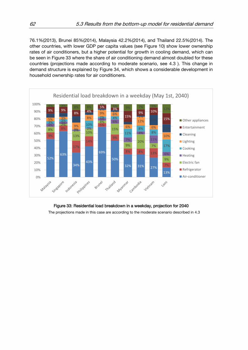
62 5.3 Results from the bottom-up model for residential demand
76.1%(2013), Brunei 85%(2014), Malaysia 42.2%(2014), and Thailand 22.5%(2014). The
other countries, with lower GDP per capita values (see Figure 10) show lower ownership
rates of air conditioners, but a higher potential for growth in cooling demand, which can
be seen in Figure 33 where the share of air conditioning demand almost doubled for these
countries (projections made according to moderate scenario, see 4.3 ). This change in
demand structure is explained by Figure 34, which shows a considerable development in
household ownership rates for air conditioners.
Figure 33: Residential load breakdown in a weekday, projection for 2040
The projections made in this case are according to the moderate scenario described in 4.3
52%63%
34%43%
69%
50%
32% 31% 27%
13%
9%
8%
17%
14%
5%
9%
8% 8% 13%
7%
8%
2%
13%10%
4%
15%
9%20%
7%
9%
4%3%
2% 0%
3%6%
7%
4%
11%
6%
3% 3%
0%
10%
2% 4%
11%8%
8%
17%
5% 3%
9%
8%9% 6%
6%
12%
6%
10%
6% 5%9%
3%2% 2%
4%
1%14%
11%
9% 9%8% 4%
5%3%
15%9% 10%
15%
4% 3% 8% 8%1% 5% 9% 7% 5%
12%
0%
10%
20%
30%
40%
50%
60%
70%
80%
90%
100%
Residential load breakdown in a weekday (May 1st, 2040)
Other appliances
Entertainment
Cleaning
Lighting
Cooking
Heating
Electric fan
Refrigerator
Air-conditioner
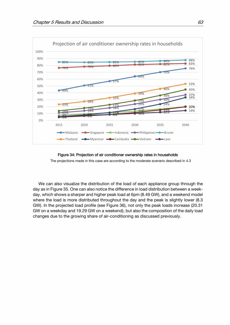
Chapter 5 Results and Discussion 63
Figure 34: Projection of air conditioner ownership rates in households
The projections made in this case are according to the moderate scenario described in 4.3
We can also visualize the distribution of the load of each appliance group through the
day as in Figure 35. One can also notice the difference in load distribution between a week-
day, which shows a sharper and higher peak load at 6pm (8.49 GW), and a weekend model
where the load is more distributed throughout the day and the peak is slightly lower (8.3
GW). In the projected load profile (see Figure 36), not only the peak loads increase (20.31
GW on a weekday and 19.29 GW on a weekend), but also the composition of the daily load
changes due to the growing share of air-conditioning as discussed previously.
44%
51%
57%
64%70%
76%76% 78% 80% 81% 82% 83%
8% 9% 11% 14%16%
20%
11%14%
18%24%
30%
37%
85% 85% 85% 85% 86% 88%
23%28%
33%39%
46%
53%
5% 8%11%
17%
24%
34%
5% 6% 8%11%
15%20%
14%18%
23%29%
36%
45%
5% 7% 8% 10% 12% 14%
0%
10%
20%
30%
40%
50%
60%
70%
80%
90%
100%
2015 2020 2025 2030 2035 2040
Projection of air conditioner ownership rates in households
Malaysia Singapore Indonesia Philippines Brunei
Thailand Myanmar Cambodia Vietnam Laos
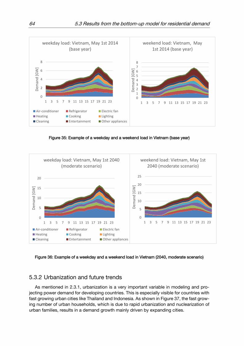
64 5.3 Results from the bottom-up model for residential demand
Figure 35: Example of a weekday and a weekend load in Vietnam (base year)
Figure 36: Example of a weekday and a weekend load in Vietnam (2040, moderate scenario)
5.3.2 Urbanization and future trends
As mentioned in 2.3.1, urbanization is a very important variable in modeling and pro-
jecting power demand for developing countries. This is especially visible for countries with
fast growing urban cities like Thailand and Indonesia. As shown in Figure 37, the fast grow-
ing number of urban households, which is due to rapid urbanization and nuclearization of
urban families, results in a demand growth mainly driven by expanding cities.
0
2
4
6
8
1 3 5 7 9 11 13 15 17 19 21 23
Dem
and
[G
W]
weekday load: Vietnam, May 1st 2014 (base year)
Air-conditioner Refrigerator Electric fan
Heating Cooking Lighting
Cleaning Entertainment Other appliances
012345678
1 3 5 7 9 11 13 15 17 19 21 23
Dem
and
[G
W]
weekend load: Vietnam, May 1st 2014 (base year)
0
5
10
15
20
1 3 5 7 9 11 13 15 17 19 21 23
Dem
and
[G
W]
weekday load: Vietnam, May 1st 2040 (moderate scenario)
Air-conditioner Refrigerator Electric fan
Heating Cooking Lighting
Cleaning Entertainment Other appliances
0
5
10
15
20
25
1 3 5 7 9 11 13 15 17 19 21 23
Dem
and
[G
W]
weekend load: Vietnam, May 1st 2040 (moderate scenario)
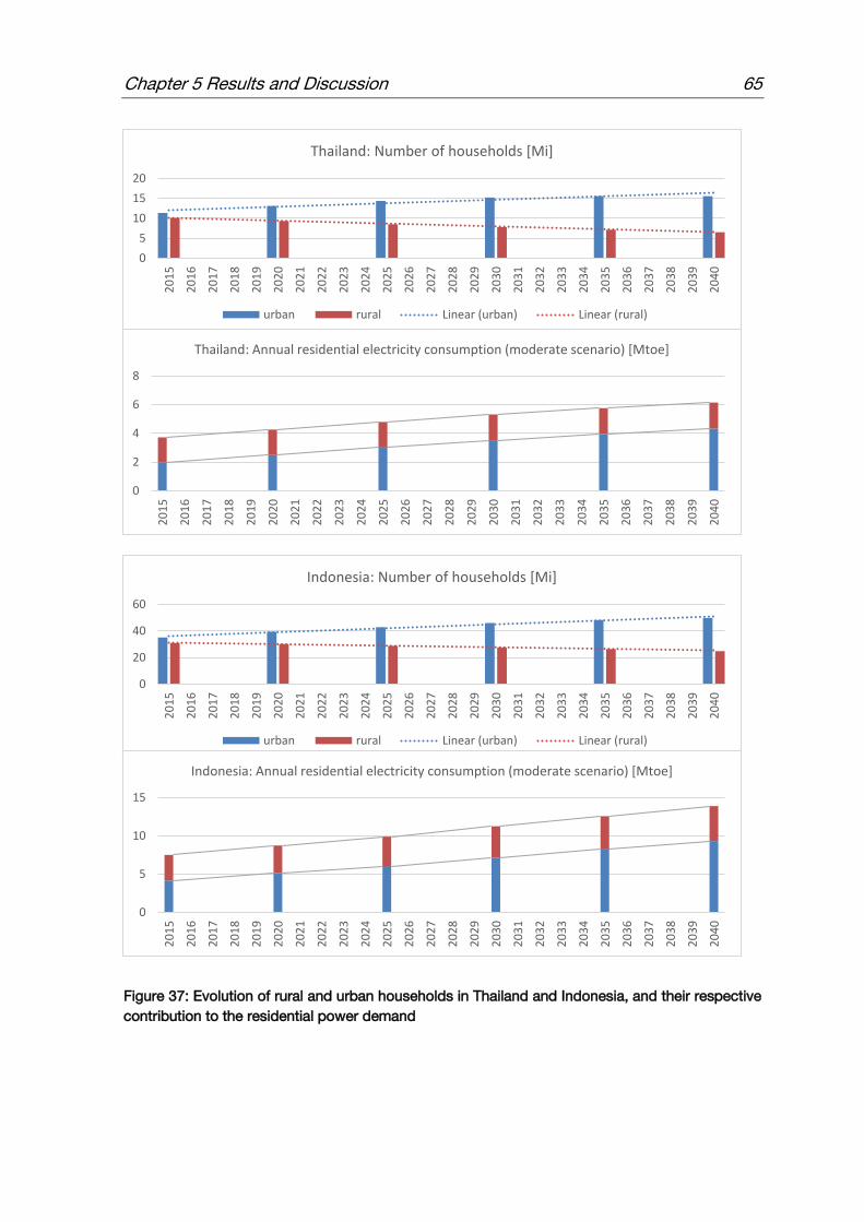
Chapter 5 Results and Discussion 65
Figure 37: Evolution of rural and urban households in Thailand and Indonesia, and their respective
contribution to the residential power demand
0
5
10
15
202
01
5
20
16
20
17
20
18
20
19
20
20
20
21
20
22
20
23
20
24
20
25
20
26
20
27
20
28
20
29
20
30
20
31
20
32
20
33
20
34
20
35
20
36
20
37
20
38
20
39
20
40
Thailand: Number of households [Mi]
urban rural Linear (urban) Linear (rural)
0
2
4
6
8
20
15
20
16
20
17
20
18
20
19
20
20
20
21
20
22
20
23
20
24
20
25
20
26
20
27
20
28
20
29
20
30
20
31
20
32
20
33
20
34
20
35
20
36
20
37
20
38
20
39
20
40
Thailand: Annual residential electricity consumption (moderate scenario) [Mtoe]
0
20
40
60
20
15
20
16
20
17
20
18
20
19
20
20
20
21
20
22
20
23
20
24
20
25
20
26
20
27
20
28
20
29
20
30
20
31
20
32
20
33
20
34
20
35
20
36
20
37
20
38
20
39
20
40
Indonesia: Number of households [Mi]
urban rural Linear (urban) Linear (rural)
0
5
10
15
20
15
20
16
20
17
20
18
20
19
20
20
20
21
20
22
20
23
20
24
20
25
20
26
20
27
20
28
20
29
20
30
20
31
20
32
20
33
20
34
20
35
20
36
20
37
20
38
20
39
20
40
Indonesia: Annual residential electricity consumption (moderate scenario) [Mtoe]

66 5.4 Results from top-down model and overall demand projection
5.4 Results from top-down model and overall demand projection
5.4.1 Final demand estimates
All the results presented in this subsection are calculated according to the moderate
scenario (see 4.3). The projected per capita demand for each of the sectors are repre-
sented in appendix E). Using these results and recalculating for the whole countries ac-
cording to the respective population estimates yields to the following demand projections:
Figure 38: Overall final demand projections for Malaysia (moderate scenario)
Figure 39: Overall final demand projections for Singapore (moderate scenario)
0.00
50.00
100.00
150.00
200.00
250.00
300.00
350.00
400.00
1990 1997 2004 2011 2018 2025 2032 2039An
nu
al E
lect
rici
ty D
eman
d [
TWh
]
Malaysia
Residential Service Industry Other
0.00
10.00
20.00
30.00
40.00
50.00
60.00
70.00
80.00
1990 1997 2004 2011 2018 2025 2032 2039An
nu
al E
lect
rici
ty D
eman
d [
TWh
]
Singapore
Residential Service Industry Other
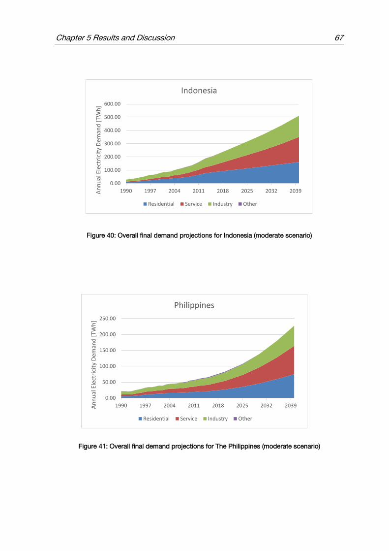
Chapter 5 Results and Discussion 67
Figure 40: Overall final demand projections for Indonesia (moderate scenario)
Figure 41: Overall final demand projections for The Philippines (moderate scenario)
0.00
100.00
200.00
300.00
400.00
500.00
600.00
1990 1997 2004 2011 2018 2025 2032 2039An
nu
al E
lect
rici
ty D
eman
d [
TWh
]Indonesia
Residential Service Industry Other
0.00
50.00
100.00
150.00
200.00
250.00
1990 1997 2004 2011 2018 2025 2032 2039An
nu
al E
lect
rici
ty D
eman
d [
TWh
]
Philippines
Residential Service Industry Other
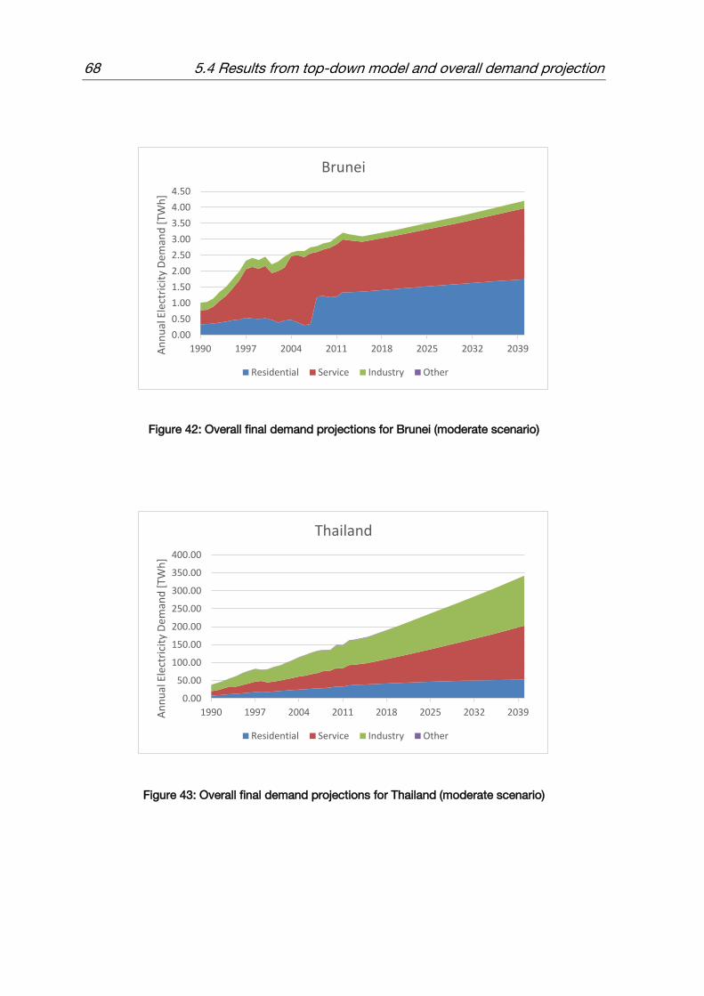
68 5.4 Results from top-down model and overall demand projection
Figure 42: Overall final demand projections for Brunei (moderate scenario)
Figure 43: Overall final demand projections for Thailand (moderate scenario)
0.00
0.50
1.00
1.50
2.00
2.50
3.00
3.50
4.00
4.50
1990 1997 2004 2011 2018 2025 2032 2039An
nu
al E
lect
rici
ty D
eman
d [
TWh
]Brunei
Residential Service Industry Other
0.00
50.00
100.00
150.00
200.00
250.00
300.00
350.00
400.00
1990 1997 2004 2011 2018 2025 2032 2039An
nu
al E
lect
rici
ty D
eman
d [
TWh
]
Thailand
Residential Service Industry Other

Chapter 5 Results and Discussion 69
Figure 44: Overall final demand projections for Myanmar (moderate scenario)
Figure 45: Overall final demand projections for Cambodia (moderate scenario)
0.00
5.00
10.00
15.00
20.00
25.00
30.00
35.00
40.00
45.00
1990 1997 2004 2011 2018 2025 2032 2039An
nu
al E
lect
rici
ty D
eman
d [
TWh
]Myanmar
Residential Service Industry Other
0.00
5.00
10.00
15.00
20.00
25.00
1990 1997 2004 2011 2018 2025 2032 2039An
nu
al E
lect
rici
ty D
eman
d [
TWh
]
Cambodia
Residential Service Industry Other
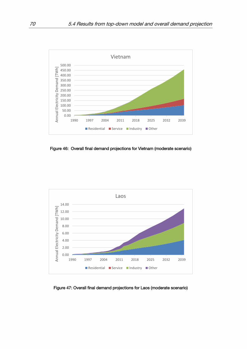
70 5.4 Results from top-down model and overall demand projection
Figure 46: Overall final demand projections for Vietnam (moderate scenario)
Figure 47: Overall final demand projections for Laos (moderate scenario)
0.00
50.00
100.00
150.00
200.00
250.00
300.00
350.00
400.00
450.00
500.00
1990 1997 2004 2011 2018 2025 2032 2039An
nu
al E
lect
rici
ty D
eman
d [
TWh
]Vietnam
Residential Service Industry Other
0.00
2.00
4.00
6.00
8.00
10.00
12.00
14.00
1990 1997 2004 2011 2018 2025 2032 2039An
nu
al E
lect
rici
ty D
eman
d [
TWh
]
Laos
Residential Service Industry Other

Chapter 5 Results and Discussion 71
The average annual growth rates in five-years-intervals are also represented in Table
12. A similar behavior to the average annual growth rates estimates of the GDP (Table 10)
and the population (Table 11) can be seen. Less developed countries will sustain a high
growth rate in electricity demand until 2040, especially Myanmar 6.1%, Cambodia 3.6%
and The Philippines 4.8%. The demand development shows therefore an exponential be-
havior for these countries (see Figure 41, Figure 44, Figure 45). Indonesia, Vietnam and
Laos are growing considerably but with a more moderate annual growth rate which will
reach around 3% by 2040. Their schematized growth shows a linear behavior in Figure 40,
Figure 46, Figure 47. On the other side, Singapore, which is a developed country, is reach-
ing a saturation level (clearly seen in Figure 39) where the electricity demand growth be-
tween 2030 and 2040 is constantly around 0.7% per year. Malaysia and Thailand are still
developing countries showing a linear growth in electricity demand until 2040 (visible in
Figure 38 and Figure 43). However, these two countries are slowly developing to a satura-
tion state similar to Singapore, where the annual growth rate by 2040 is around 2.5% which
is the same as Singapore between 2015 and 2020. Brunei, on its side, is a very unique
case since it showed some instabilities in the past (see Figure 42) which makes it more
unpredictable. The estimates for Brunei show hence a slow growth with a constant rate
around 1.2%.
Historic data Estimates
Country 1990 - 1995
1995 - 2000
2000 - 2005
2005 - 2010
2010 - 2015
2015 - 2020
2020 - 2025
2025 - 2030
2030 - 2035
2035 - 2040
Malaysia 14.5% 9.3% 5.7% 6.5% 4.7% 5.3% 4.0% 3.5% 3.1% 2.7%
Singapore 7.1% 8.3% 5.4% 3.3% 2.9% 2.5% 1.4% 1.3% 0.7% 0.7%
Indonesia 12.0% 9.7% 6.4% 6.6% 6.7% 4.8% 4.0% 3.4% 3.2% 3.1%
Philippines 4.6% 6.6% 4.3% 4.1% 3.3% 5.0% 5.2% 5.4% 5.3% 4.8%
Brunei 11.7% 6.9% 1.4% 2.0% 1.2% 1.2% 1.3% 1.2% 1.3% 1.2%
Thailand 13.2% 4.3% 6.6% 4.3% 2.8% 3.4% 3.1% 2.7% 2.4% 2.3%
Myanmar 6.4% 6.7% 2.3% 11.4% 5.4% 6.7% 6.5% 6.5% 6.3% 6.1%
Cambodia - 26.1% 17.6% 18.9% 12.6% 10.4% 7.8% 5.7% 5.6% 5.6%
Vietnam 12.6% 14.9% 16.0% 13.0% 8.9% 8.2% 6.0% 3.9% 3.7% 3.6%
Laos 15.4% 13.6% 9.6% 17.1% 11.6% 9.3% 4.8% 3.7% 3.6% 3.5%
Table 12: Final electricity demand average annual growth rates (aagr)
Historic data from (IEA, 2016)
The absolute final annual electricity consumption is presented in Figure 48. The figure
shows the estimated growth for the region in terms of electricity consumption which ac-
counts to around 159%. It also shows that the largest electricity consumers of Southeast
Asia will be Indonesia, Malaysia, Vietnam and Thailand followed by The Philippines.

72 5.4 Results from top-down model and overall demand projection
Figure 48: Final electricity demand in ASEAN: history and estimates
Historical data from (IEA, 2016)
0.00
500.00
1000.00
1500.00
2000.00
2500.00
19
90
19
92
19
94
19
96
19
98
20
00
20
02
20
04
20
06
20
08
20
10
20
12
20
14
20
16
20
18
20
20
20
22
20
24
20
26
20
28
20
30
20
32
20
34
20
36
20
38
20
40
Fin
al a
nn
ual
ele
ctri
city
dem
and
[TW
h]
ASEAN final annual electricity demand
Malaysia Singapore Indonesia Philippines Brunei
Thailand Myanmar Cambodia Vietnam Laos

Chapter 5 Results and Discussion 73
One more important observation is concerning the contribution of each sector to the
final electricity demand. As shown in Figure 49, the share of households’ consumption
decreases from 30% in 2015 (for all ASEAN) to 24% in 2040. On the other hand, the con-
tribution of the service sector to the final demand increases from 27% in 2015 to 34% in
2040. This behavior, as discussed in 2.3 and 3.2.4, is expected in developing countries,
since at an early stage of development, the residential sector is dominant in electricity
consumption, and as long as the economy grows, the consumption from industry and ser-
vice sectors increases. It is also discussed in 2.3.1 that developing countries would not
necessarily through the traditional path of industrialization and consequently developing
the service sector, but can “leapfrog” developed countries through directly achieving
growth in service-oriented activities.
Figure 49: Sectors contribution to the final electricity demand estimates in 2015 and 2040
21% 16%
41% 32%44%
23% 28%48%
34% 37%
32% 43%
25%31%
51%
35% 21%
29%
9% 0%
47% 40% 34% 34%
5%
42%
33%
20%
56%
34%
0% 1% 1% 3% 0% 1%18%
3% 1%
29%
0%
20%
40%
60%
80%
100%
120%
Sector contribution to final electricity demand (2015)
Residential Service Industry Other
15% 14%31% 33% 42%
15%
44% 36%22%
32%
42% 46%
37% 39%
53%
44%
25% 39%
14% 0%
43% 40% 32% 28%
6%
41% 24%24%
64%
37%
0% 0% 0% 0% 0% 0% 7% 0% 0%
31%
0%
20%
40%
60%
80%
100%
120%
Sector contribution to final electricity demand (2040)
Residential Service Industry Other

74 5.5 Generated power load profiles
5.4.2 Scenario analysis
Results according to the scenarios described in 4.3 are represented in Figure 50 (more
in detail for each country in appendix I)). Demand forecasting is a complex task and highly
linked to uncertainties since the result may depend on exogenous factors to the modeled
system (e.g. applied policies). The two “extreme” scenarios 2 and 3 are meant therefore to
introduce an interval to which the final value is expected to belong. The most important
variable here is efficiency, where scenario 1 assumes a slow improvement in efficiency,
scenario 2 assumes an active and fast efficiency improvement, and scenario 3 assumes
no improvement accompanied with a higher growth. This points out the importance of
energy efficiency measures especially in a fast growing region as ASEAN in order to curb
the highly increasing power demand.
Figure 50: Demand scenarios for the whole ASEAN region
5.5 Generated power load profiles
The final goal of the model is to generate overall power load profiles in hour resolution.
Figure 51 shows an example of the generated load profiles with the separate contribution
of each sector. The first plot is from the Vietnam model (2015) and shows the load profile
of a working day. The second plot is from the Malaysia model (2015) and shows the load
for several days, where it is visible that weekend days have a lower peak.
174.44
131.07
202.48
0.00
50.00
100.00
150.00
200.00
250.00
19
90
19
92
19
94
19
96
19
98
20
00
20
02
20
04
20
06
20
08
20
10
20
12
20
14
20
16
20
18
20
20
20
22
20
24
20
26
20
28
20
30
20
32
20
34
20
36
20
38
20
40
Tota
l dem
and
[M
toe]
Demand scenarios
Scenario 1 Scenario 2 Scenario 3 Historic data
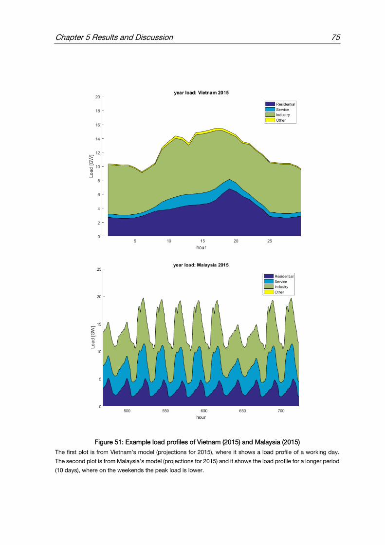
Chapter 5 Results and Discussion 75
Figure 51: Example load profiles of Vietnam (2015) and Malaysia (2015)
The first plot is from Vietnam’s model (projections for 2015), where it shows a load profile of a working day.
The second plot is from Malaysia’s model (projections for 2015) and it shows the load profile for a longer period
(10 days), where on the weekends the peak load is lower.

76 5.5 Generated power load profiles
Figure 52: Comparison between the load profile for Singapore and Cambodia
The first plot is from Cambodia’s model (projections for 2015) and the second plot is from Singapore’s model
(projections for 2015). While the first profile shows a sharp evening peak due to the residential load, the second
profile is more uniform with a high load during the day due to the industrial and service related loads.

Chapter 5 Results and Discussion 77
Not only the magnitude of the daily peak differs between the generated load profiles for
different countries, but also the shape of the profile due to differences in the power supply
structure, which is in its turn due to differences in development level (see 3.2.4). For exam-
ple, Figure 52 compares between the load profile in Singapore and Cambodia. The load
profile for Singapore shows a higher magnitude during the day and a larger difference
between a weekday and a weekend, due to the large contribution of industry and service
sectors. For Cambodia, however, the peak load is mainly caused by the residential evening
peak, and there is a smaller difference in magnitude between a weekday and a weekend.
A similar behavior is observed with actual data as shown in appendix F). The structure of
power supply is obviously expected to change in the future as the industry and service
sectors grow. This is seen for example in Figure 53 for The Philippines, where the load
profile develops from the traditional residential evening peak to a midday high load.
Figure 53: Generated load profile of The Philippines in 2015 (left) and in 2040 (right)
One more feature which can be visualized through load profiles is the correlation to the
temperature profile. As already mentioned, the cooling load accounts for an important
share of the overall power consumption. Since the cooling power is modeled as a function
of the temperature and the humidity, a clear correlation can be seen between the power
load profile and the temperature profile. As represented in Figure 54, Malaysia, which has
a rather uniform temperature profile during the whole year, shows also a uniform power
consumption profile. However, Vietnam, where temperature is lower during winter season,
shows lower power consumption in the same season.

78 5.5 Generated power load profiles
Figure 54: Correlation between power load and temperature
Power load profile (green) and temperature load profile (blue) for Malaysia (up) and Vietnam (down) for the
whole year (2015 projections)

Chapter 6 Conclusions 79
6 Conclusions
In this study a hybrid bottom-up and top-down power demand model is developed in
order to deliver projections for the annual power demand and the corresponding load pro-
files in hour resolution. The model is applied for all ASEAN nations (10 countries). An end-
use (bottom-up) model is developed for the residential sector, since it’s the most homoge-
neous and uniform sector and can be modeled similarly for all the countries. An econo-
metric (top-down) model is developed for the three other sectors (industry, service, other),
taking into consideration the structural differences between the modeled sectors. As pro-
jection variables, the end-use model takes into consideration socio-economic (population,
GDP, urbanization, electrification) as well as technology related (technology diffusion, effi-
ciency improvement) factors. The econometric model relies on the observation that spe-
cific power consumption growth decreases with increasing economic development. The
correlation is performed with time series data from different countries, and the projections
follow power functions. Power load profiles in hour resolution are generated from both
models for the total electricity consumption. The generated load comprises an HVAC
share, wish is calculated in accordance with the meteorological characteristics of the mod-
eled region.
Modeling electricity demand for ASEAN countries is linked to many challenges, mainly
the structural differences between the countries and the data scarcity to different extents
for each of them. The model, however, for the sake of consistency, should be uniform and
applicable to each of the modeled countries in the same way. The developed model in this
study is flexible in a way to be applicable for all ASEAN regions and sub-regions, and can
even be extended for further countries. The detail level in modeling is kept enough to match
the available data and additionally deliver quite accurate results (projected load profiles)
usable for further power system optimization simulations.
The outcomes of the model point out the importance of the overall growth expected in
the ASEAN region which will be clearly reflected in electricity demand (up to 182% growth
between 2013 and 2040 in the moderate scenario). This growth trend is not distributed
evenly between ASEAN nations, due to the actual present gaps in development. Singa-
pore, which is the most developed country of ASEAN, already reached a nearly saturated
level and will know an average annual growth rate in power consumption of 1.3%. Brunei,
which is the second richest country in the region (in terms of GDP/cap), also shows a low
growth around 1.2% per year. Malaysia and Thailand, the next on the development ladder,
expect a considerable growth in the future around 3.7% and 2.8% per year respectively.
This growth is however slowing down, which means that they are on the way to reaching
saturation levels in the further future. The least developed countries are the ones which are
expecting the highest growth rates in power consumption, especially Cambodia with 7%
per year and Myanmar with 6.4% per year. In terms of absolute electricity consumption,
Indonesia will be the largest consumer with 25.2% of the total ASEAN power consumption
in 2040, followed by Vietnam with 22.7%, Malaysia 17.0%, Thailand 16.9% and The Phil-
ippines 11.2%. The total electricity consumption of ASEAN will be around 174.43 Mtoe
according to the moderate scenario. On the other hand, the results of the end-use model
point out the importance of the air-conditioning load in this region. In the residential sector
for example, the air-conditioning load will grow from 27.6% from the total load in 2014 (all
ASEAN) to 38.6% in 2040 according to the moderate scenario.
80 5.5 Generated power load profiles
All this expected growth gives rise not only to the necessity of building additional power
capacity, but also to the discussion about the quality of power generation in terms of effi-
ciency and emissions. Energy efficiency (EE) measures implementation is crucial for the
fast growing region since it curbs demand growth (as shown in scenario 2) and therefore
reduces additional power capacity needs. EE measures also through reducing consump-
tion will lower fossil fuel imports and therefore expenditures on fossil fuel subsidies and
contribute to the nations’ prosperity and energy security. And because of the important
share of cooling in the final demand, applying EE measure to air-conditioning appliances
can be a valuable investment. On the other hand, a growing demand translates also to
growing emissions. It is therefore important to reduce the high dependence on fossil fuels
through gradual integration of renewable energies, especially that the region has a large
untapped potential for renewable sources. All these measures should be supported with
consistent policies which aim to increase energy efficiency in the region and partake in
reducing global emissions.
The future work within this project, is to use the generated power load profiles with the
developed model in order to match the demand to the supply of renewable energy sources
(solar, wind, hydro, geothermic etc.) and optimize the overall energy system with the aim
of integrating more renewables/ reducing emissions.

References & Appendices i
References
ADB, 2013. Energy Outlook for Asia and the Pacific, Manila: Asian Development Bank.
ADB, 2014. ASEAN 2030: Toward a Borderless Economic Community, Japan: Asian
Development Bank Institute.
ADB, 2014. Keynote speech: ASEAN Integration and the Private Sector - Stephen P.
Groff. [Online]
Available at: www.adb.org/news/speeches/keynote-speech-asean-integration-and-private-
sector-stephen-p-groff
[Accessed August 2016].
Ahmad, A. & Othman, H. M., 2014. Electricity Consumption in Brunei Darussalam:
Challenges in Energy Conservation. International Energy Journal, Issue 14, pp. 155 - 166.
AITI, 2010. Brunei Darussalam Household ICT Survey Report, Bandar Seri Begawan:
Authority for Info-Communications Technology Industry of Brunei Darussalam.
Al-Alawi, S. M. & Islam, S. M., 1996. Principles of electricity demand forecasting. Power
Engineering Journal 10.3 , pp. 139-143.
Alfares, H. K. & Nazeeruddin, M., 2002. Electric load forecasting: literature survey and
classification of methods. International Journal of Systems Science 33, pp. 23-34.
Almeida, A. d., 2008. Residential monitoring to decrease energy use and carbon emissions
in Europe - Report with the results of the surveys based on questionnaires for all countries,
Coimbra: University of Coimbra.
APERC, 2016. APEC Energy Demand and Supply Outlook, 6th edition, Tokyo: Asia
Pacific Energy Research Center APERC.
ASEAN, 1967. The Asean Declaration (Bangkok Declaration). Bangkok: asean.org/the-
asean-declaration-bangkok-declaration-bangkok-8-august-1967/.
ASEAN, 2015. ASEAN Economic Community. [Online]
Available at: asean.org/asean-economic-community/
[Accessed August 2016].
ASEAN, 2015. The 4th ASEAN Energy Outlook, Jakarta: ASEAN Centre for Energy.

ii References & Appendices
ASEAN, 2016. ASEAN Overview. [Online] 3
Available at: asean.org/asean/about-asean/overview/
[Accessed 2016].
ASHRAE, 2001. HVAC 2001 Fundamentals Handbook. Atlanta: ASHRAE.
Aye, M. P., 2015. Deliverable Report for MECON Project: Baseline energy consumption
of MECON household in Myanmar, Yangon: MYANMAR ENGINEERING SOCIETY.
Bass, F. M., 1969. A New Product Growth Model for Consumer Durables. Management
Science, 15(5), pp. 215-227.
Berk, K., 2015. Modeling and Forecasting Electricity Demand: A Risk Management
Perspective. Wiesbaden: Springer Spektrum.
Berrah, N., Feng, F., Priddle, R. & Wan, L., 2007. Sustainab leEnergy in China: The
Closing Window of Opportunity, Washington ,D.C.: The World Bank.
Bhattacharyya, S. C. & Timilsina, G. R., 2009. Energy Demand Models for Policy
Formulation, A Comparative Study of Energy Demand Models, s.l.: The World Bank.
Bhattacharyya, S. C. & Timilsina, G. R., 2010. Modelling energydemand of developing
countries: Are the specific features adequately captured?. Energy Policy.
Blackman, A. W., 1972. A Mathematical Model for Trend Forecasts. Technological
Forecasting and Social Change, Issue 3, pp. 441-452.
Chang, Y. & Li, Y., 2012. Power Generation and Cross-border Grid Planning for the
Integrated ASEAN Electricity Market: A Dynamic Linear Programming Model, Jakarta:
Economic Research Institute for ASEAN and East Asia ERIA.
Chateau, B. & Lapillonne, B., 1978. Long-term energy demand forecasting, a new
approach. Energy Policy, 6(2), pp. 140 - 157.
Chen, H., Canizares, C. & Singh, A., 2001. ANN-Based Short-Term. s.l., IEEE, p. 11–415.
Das, S. B., Menon, J., Severino, R. & Shrestha, O. L., 2013. The ASEAN Economic
Community: A Work in Progress. Singapore: Institute of South East Asian Studies.
Department Of Electrical Services, 2013. HAPUA WORKING COMMITTEE MEETING
Report, Phnom Penh: Department Of Electrical Services.
Department of Statistics Malaysia, 2010. Laporan Kiraan Permulaan, Kuala Lumpur:
Department of Statistics Malaysia.

References & Appendices iii
Department of Statistics Malaysia, 2014. Report of Household Income and Basic Amenities
Survey, Kuala Lumpur: Department of Statistics Malaysia.
Department of Statistics Singapore, 2013. Household Expenditure Survey 2012/13,
Singapore: Department of Statistics Singapore.
Department of Statistics Singapore, 2015. Singapore Census of Population 2015,
Singapore: Department of Statistics Singapore.
DIN EN 15251, 2007. DIN EN 15251, Eingangsparameter für das Raumklima
(Raumluftqualität, Temperatur, Licht und Akustik), Berlin: DIN Deutsches Institut für
Normung.
DLR, 2005. Concentrating Solar Power for the Mediterranean Region, Stuttgart: German
Aerospace Center (DLR).
DoE, 2014. Department of Energy - Electric Power Statistics. [Online]
Available at: www.doe.gov.ph/electric-power-statistics/philippine-power-statistics
[Accessed June 2016].
EAC, 2015. Report on Power Sector of the Kingdom of Cambodia, Phnom Penh:
Electricity Authority of Cambodia.
EDC, 2012. Annual Report 2012, Phnom Penh: Electricite du Cambodge.
EDL, 2015. ELECTRICITE DU LAOS - Contact. [Online]
Available at: edl.com.la
[Accessed Mai 2015].
EIA, 2011. RESIDENTIAL ENERGY CONSUMPTION SURVEY. [Online]
Available at: www.eia.gov/consumption/residential/reports/2009/air-conditioning.cfm
[Accessed August 2016].
EMA, 2016. Energy Market Authority. [Online]
Available at: www.ema.gov.sg
[Accessed January 2015].
ENERGY STAR, 2011. ENERGY STAR Market & Industry Scoping Report - Vacuum
Cleaners, s.l.: ENERGY STAR.
EPA, 2015. End-Users of Electricity. [Online]
Available at: www.epa.gov/energy/end-users-electricity
[Accessed August 2016].
iv References & Appendices
EPPO, 2015. Energy Statisics of Thailand 2015, Bangkok: Energy Policy and Planning
Office.
ERAV, 2015. Electricity Regulatory Authority of Vietnam. [Online]
Available at: www.erav.vn
[Accessed Mai 2015].
ESDM, 2008. Handbook of Energy & Economics Statistics of Indonesia. [Online]
Available at: www.esdm.go.id/publikasi/statistik/handbook.html
[Accessed June 2016].
Eto, J. et al., 1990. Analysis of California Hourly End-Use Residential Electricity Load
Shapes, Berkley, California: Lawrence Berkley Laboratory.
Evenson, R. E. & Westphal, L. E., 1995. Technological change and technology strategy.
In: Handbook of development economics. Amsterdam: North-Holland, p. 2209–2300.
Fagerberg, J. & Verspagen, B., 2002. Technology-gaps, innovation-diffusion and
transformation: an evolutionary interpretation. Research Policy, Issue 31, pp. 1291-1304.
Feinberg, E. A. & Genethliou, D., 2005. Load forecasting. In: Applied mathematics for
restructured electric power systems: Optimization, control, and computational
intelligence. New York: Springer, pp. 269-285.
Fisher, J. & Pry, R., 1971. Simple Substitution Model of Technological Change.
Technological Forecasting and Social Change, Issue 3, pp. 75-88.
General Statistics Office, 2015. The 2014 Viet Nam Intercensal Population and Housing
Survey: Major Findings, Hanoi: General Statistics Office.
GeoData, 2016. WorldPop. [Online]
Available at: www.worldpop.org.uk
[Accessed June 2016].
GES DISC, 2015. The Modern-Era Retrospective analysis for Research and Applications
(MERRA data). s.l.:Goddard Earth Sciences Data and Information Center (GES DISC) and
Global Modeling and Assimilation Office (GMAO).
Gruebler, A., Nakicenovic, N. & Victor, D. G., 1999. Dynamics of energy technologies
and global change. Energy policy, Issue 27, pp. 247 - 280.
Hahn, H., Meyer-Nieberg, S. & Pickl, S., 2009. Electric load forecasting methods: Tools
for decision making. European Journal of Operational Research 199, p. 902–907.

References & Appendices v
Hainoun, A., Seif-Eldin, M. & Almoustafa, S., 2006. Analysis of the Syrian long-term
energy and electricity demand projection using the end-use methodology. Energy Policy,
Issue 34, pp. 1958 - 1970.
Heaps, C., 2012. Long-range Energy Alternatives Planning (LEAP) system. [Online]
Available at: www.energycommunity.org
Hendron, R. & Engebrecht, C., 2010. Building America House Simulation Protocols, s.l.:
National Renewable Energy Laboratory.
Herzog, S. & Hamacher, T., 2016. Economic evaluation of battery storages in context of
system size. Dusseldorf, 10th International Renewable Energy Storage Conference .
Hoekman, B. M., Maskus, K. E. & Saggi, K., 2005. Transfer of Technology to Developing
Countries: Unilateral and Multilateral Policy Options. World Development , 33(10), pp.
1587-1602.
Huber, M., Roger, A. & Hamacher, T., 2015. Optimizing long-term investments for a
sustainable development of the ASEAN power system. Energy, Issue 88, pp. 180-193.
Hulme, J., Beaumont, A. & Summers, C., 2013. Domestic appliances, cooking & cooling
equipment, London: Department of Energy and Climate Change.
IAEA, 2006. Model for analysis of energy demand (MAED -2), Vienna: International
Atomic Energy Agency.
IEA, 2015. Southeast Asia Energy Outlook 2015, Paris: International Energy Agency.
IEA, 2015. World Energy Outlook 2015– Electricity Access Database. [Online]
Available at: www.worldenergyoutlook.org
[Accessed 2016].
IEA, 2016. Electricity and heat statistics. [Online]
Available at: www.iea.org/statistics/statisticssearch/
[Accessed August 2016].
Immigration and Manpower Department, 1986. 1983 Population Census, Rangoon:
Immigration and Manpower Department.
Iniyana, S., Suganthib, L. & Samuel, A. A., 2006. Energy models for commercial energy
prediction and substitution of renewable energy sources. Energy Policy, Issue 34, pp. 2640
- 2653.

vi References & Appendices
Ishiguro, M. & Akiyama, T., 1995. Energy Demand in Five Major Asian Developing
Countries, Washington DC: World Bank Discussion Papers 277, World Bank.
Jakob, M., Kallio, S. & Bossman, T., 2014. Generating electricity demand-side load
profiles of the tertiary sector for selected European countries. Frankfurt, 8th International
Conference Improving Energy Efficiency in Commercial Buildings.
Kamsamrong, J., 2015. Deliverable Report for MECON Project: Baseline energy
consumption of MECON household in Thailand, Bangkok: King Mongkut’s University of
Technology Thonburi.
Kamsamrong, J., 2015. Deliverable Synthesis Report for MECON Project - Task 1.2:
Baseline energy consumption of MECON household, Hanoi: Hanoi University of Science
and Technology.
Karali, N., McNeil, M. A., Letschert, V. & Can, S. d. l. R. d., 2015. Potential Impact of
Lighting and Appliance Efficiency Standards on Peak Demand: The Case of Indonesia,
Berkley: Ernest Orlando Lawrence Berkley National Laboratory.
Koomey, J., 2000. From my perspective: avoiding "the Big Mistake" in forecasting
technology adoption. Berkeley, Ernest Orlando Lawrence Berkeley National Laboratory.
Kutani, I. & Li, Y., 2014. Investing in Power Grid Interconnection in East Asia, Jakarta:
Economic Research Institute for ASEAN and East Asia ERIA.
LaCommare, K. H. et al., 2002. Investigation of Residential Central Air Conditioning Load
Shapes in NEMS, Berkeley: Ernest Orlando Lawrence Berkeley National Laboratory.
Lao Statistics Bureau, 2012. Lao Social Indicator Survey, Vientiane: Lao Statistics Bureau.
Lapillonne, B., 2015. Households indicators, Bogota: UPME.
Letschert, V. E. & McNeil, M. A., 2009. Material world: forecasting household appliance
ownership in a growing global economy. Berkeley, Lawrence Berkeley National
Laboratory.
Lidula, N. et al., 2007. ASEAN towards clean and sustainable energy: Potentials,
utilization and barriers. Renewable Energy, Volume 32, pp. 1441-1452.
Lucas, K., 2006. Thermodynamik: Grundgesetze der Energie- und Stoffumwandlungen.
Berlin: Springer.

References & Appendices vii
Mansfield, E., 1961. Technical Change and the Rate of Imitation. Econometrica, 29(4), pp.
741 - 766.
Martino, J., 1975. Technological Forecusring for Decision Making. New York: American
Elsevier.
Masilmani, L. & Peterson, J., 2014. The “ASEAN Way”: The Structural Underpinnings of
Constructive Engagement. Foreign Policy Journal, pp. 1-21.
McNeil, M. A. & Letschert, V. E., 2005. Forecasting Electricity Demand in Developing
Countries: A Study of Household Income and Appliance Ownership. Mandelieu, France,
European Council for an Energy Efficient Economy-2005 Summer Study.
McNeil, M. A. & Letschert, V. E., 2010. Modeling diffusion of electrical appliances in the
residential sector, Berkeley: Ernest Orlando Lawrence Berkeley National Laboratory.
Mehra, M. K. & Bharadwaj, A. G., 2000. Demand Forecasting for Electricity. New Delhi,
s.n.
Miller, N. L., Hayhoe, K., Jin, J. & Auffhammer, M., 2006. Climate, Extreme Heat, and
Electricity Demand in California. Journal of Applied Meteorology and Climatology.
Ministry of Immigration and Population, 2015. The 2014 Myanmar Population and
Housing Census - The Union Report, Naypyidaw: Ministry of Immigration and Population.
Morna, I. & van Vuuren, D. P., 2009. Modeling global residential sector energy demand
for heating and air conditioning in the context of climate change. Energy Policy, 37(2), pp.
507 - 521.
Nanthavong, K., 2006. Socio-economic survey in Lao PDR, Vientiane: National University
of Laos.
National Bureau of Statistics of China, 2015. China Statistical Yearbook, Beijing: National
Bureau of Statistics of China.
National Institute of Statistics, 2014. Cambodia Inter-Censal Population Survey 2013,
Phnom Penh: National Institute of Statistics.
National Institute of Statistics, 2015. Cambodia Socio-Economic Survey, Phnom Penh:
National Institute of Statistics.
National Statistical Office, 2013. The 2013 Household Socio-Economic Survey (Whole
Kingdom), Bangkok: National Statistical Office.
viii References & Appendices
NEA, 2012. Data Centre Energy Efficiency Benchmarking, Singapore: National
Environment Agency NEA.
NSSO, 2014. Household Consumption of Various Goods and Services in India, New
Delhi: National Sample Survey Office.
Osueke, E. C. O. & Ezeh, E. C. T., 2011. Assessment of Nigeria power sub-sector and
electricity generation projections. International Journal of Scientific & Engineering
Research, 2(11).
OTA, 1991. Energy in Developing Countries, Washington, DC: OTA-E-486,Office of
Technology Assessment. U.S.Congress, U.S. Government Printing Office.
Page, J., 2003. The Role of Solar Radiation Climatology in the Design of Photovoitaic
Systems. In: Practical Handbook of Photovoltaics: Fundamentals and Applications.
Oxford: Elsevier, pp. 6 - 65.
Pandey, R., 2002. Energy policy modeling: agenda for developing countries. Energy
Policy, Issue 30, pp. 97 - 106.
Parente, S. L. & Prescott, E. C., 1994. Barriers to technology adoption and development.
Journal of Political Economy, 2(102), pp. 298-321.
PEA, 2016. Provincial Electricity Authority - Contact. [Online]
Available at: pea.co.th/en/
[Accessed Mai 2015].
PEMC, 2012. Philippine Electricity Market Corporation - Wholesale Electricity Spot
Market. [Online]
Available at:
www.wesm.ph/inner.php/the_market/wholesale/market_data_and_reports/daily_operations
_reports/previous_day_summary/luzon_pds
[Accessed Mai 2015].
Philippine Statistics Authority, 2012. The 2010 Census of Population and Housing.
[Online]
Available at: https://psa.gov.ph/content/2010-census-population-and-housing-reveals-
philippine-population-9234-million
[Accessed June 2016].
Philippine Statistics Authority, 2013. Electricity is the most common source of energy used
by households. [Online]

References & Appendices ix
Available at: psa.gov.ph/content/electricity-most-common-source-energy-used-households
[Accessed Mai 2016].
PLN, 2014. Jawa-Bali Power Line. [Online]
Available at: hdks.pln-jawa-bali.co.id/
[Accessed Mai 2015].
Pokharel, S., 2007. Aneconometric analysis of energy consumption in Nepal. Energy
Policy, Issue 35, pp. 350 - 361.
Ponniran, A., Mamat, N. A. & Joret, A., 2012. Electricity Profile Study for Domestic and
Commercial Sectors. International Journal of Integrated Engineering, 4(3), pp. 8 - 12.
Pratt, R. G. et al., 1989. Description of Electric Energy Use in Single-Family Residences in
the Pacific Northwest, End-Use Load and Consumer Assessment Program (ELCAP).
s.l.:Bonneville Power Administration.
Scasny, M. & Urban, J., 2009. Household Behaviour and Environmental Policy:
Residential Energy Efficiency. Paris, OECD Conference on "Household Behaviour and
Environmental Policy".
Schmidt, M., Arold, J. & Klimke, K., 2010. Regelstrategien zum Verbessern der
Jahresarbeitszahl von Luft- und Wasser-Wärmepumpen, Stuttgart: Institut für
Gebäudeenergetik (IGE).
Sharif, N. & Islam, M. N., 1980. The Weibull Distribution as a General Model for
Forecasting Technological Change. Technological Forecasting and Social Change, Issue
18, pp. 247-256.
Shi, X., 2015. Application of best practice for setting minimum energy efficiency standards
in technically disadvantaged countries: Case study of Air Conditioners in Brunei
Darussalam. Applied Energy, Issue 157, pp. 1 - 12.
Somerton, C. W., 2012. Phase Change Substance Property Tables in SI Units. Michigan:
Michigan State University.
Sriv, T., Sok, K. & San, V., 2015. Deliverable Report for MECON Project Task 1.2
Baseline energy consumption of MECON household in Cambodia, Phnom Penh: Royal
University of Agriculture.
Statistics Indonesia, 2015. National Socio-Economic Survey 2015 , Jakarta: Badan Pusat
Statistik.

x References & Appendices
Statistics Indonesia, 2016. Statistics Indonesia. [Online]
Available at: http://www.bps.go.id/
[Accessed June 2016].
Statistics Japan, 2015. 2015 Population Census, Tokyo: Statistics Bueau Japan.
Stich, J. & Massier, T., 2015. Enhancing the Integration of Renewables by Trans-Border
Electricity Trade in ASEAN. s.l., IEEE PES Asia-Pacific.
Suruhanjaya Tenaga, 2011. Malaysia Energy Information Hub. [Online]
Available at: meih.st.gov.my/statistics
[Accessed June 2016].
Suruhanjaya Tenaga, 2013. Daily Logsheet (DLS) Reports 2012 (Peninsular Malaysia).
[Online]
Available at: www.st.gov.my/index.php/ms/component/content/article/12-industry/304-
daily-logsheet-dls-reports.html
[Accessed Mai 2015].
Suruhanjaya Tenaga, 2013. Sabah Grid System Operation Summary Reports 2012.
[Online]
Available at: www.st.gov.my/index.php/ms/component/content/article/12-industry/387-
sabah-grid-system-operation-summary-reports-2012.html
[Accessed Mai 2015].
Swisher, J. N., Januzzi, G. d. M. & Redlinger, R. Y., 1997. Integrated Resource Planning.
Denmark: UNEP Collaborating Center on Energy and Environment.
Tanatvanit, S., Limmeechokchai, B. & Chungpaibulpatana, S., 2003. Sustainable energy
development strategies: implications of energy demand management and renewable energy
in Thailand. Renewable and Sustainable Energy Reviews, Issue 7, p. 367–395.
UN, 1973. Methods of projecting households and families. s.l.:United Nations.
UN, 1991. Sectoral energy demand studies: Application of the end-use approach to Asian
countries, Report 33, Energy Resources Development Series, New: United Nations.
UN, 2014. World Urbanization Prospects: The 2014 Revision. [Online]
Available at: esa.un.org/unpd/wup/
[Accessed Mai 2016].

References & Appendices xi
UN, 2015. National Accounts Main Aggregates Database. [Online]
Available at: unstats.un.org/unsd/snaama/dnllist.asp
[Accessed June 2016].
UN, 2015. UN National Accounts. [Online]
Available at: unstats.un.org/unsd/snaama/dnllist.asp
[Accessed June 2016].
UN, 2015. World Population Prospects: The 2015 Revision. [Online]
Available at: esa.un.org/unpd/wpp/
[Accessed Mai 2016].
UN, 2016. UN Stats. [Online]
Available at:
unstats.un.org/unsd/demographic/sconcerns/housing/comp1995/TABLE06.pdf
[Accessed June 2016].
UNDP, 2015. Human Development Data (1980-2015). [Online]
Available at: http://hdr.undp.org/en/data
[Accessed August 2016].
UNSD, 2016. UNSD Energy Statistics Database. [Online]
Available at: unstats.un.org/unsd/energy/edbase.htm
[Accessed August 2016].
Urban, F., Benders, R. & Moll, H., 2007. Modelling energy systems for developing
countries. EnergyPolicy, Issue 35, pp. 3473 - 3482.
US EPA, 2015. End-Users of Electricity. [Online]
Available at: www.epa.gov/energy/end-users-electricity
[Accessed August 2016].
USDA, 2016. United States Department of Agriculture. [Online]
Available at: www.ers.usda.gov/media/612721/householdamenities.xls
[Accessed August 2016].
Vietnamese Team, 2015. Deliverable Report for MECON Project: Baseline energy
consumption of MECON household in Vietnam, Hanoi: Hanoi University of Science and
Technology.
Vongchanh, K., 2015. Deliverable Report for MECON Project: Baseline energy
consumption of MECON household in Lao PDR, Vientiane: National University of Laos.

xii References & Appendices
WEC, 2010. 2010 Survey of Energy Resources, London: World Energy Council.
Werbos, P. J., 1990. Econometric techniques: theory versus practice, Special issue of.
Energy, pp. 213-36.
World Bank, 2008. Residential consumption of electricity in India, s.l.: The World Bank.
World Bank, 2016. World Development Indicators. [Online]
Available at: databank.worldbank.org/
[Accessed August 2016].
Wyssen, I. et al., 2010. Effizientes Heizen und Kühlen mit Niedrighub-Anlagen. Zurich,
Status-Seminar «Forschen und Bauen im Kontext von Energie und Umwelt» .
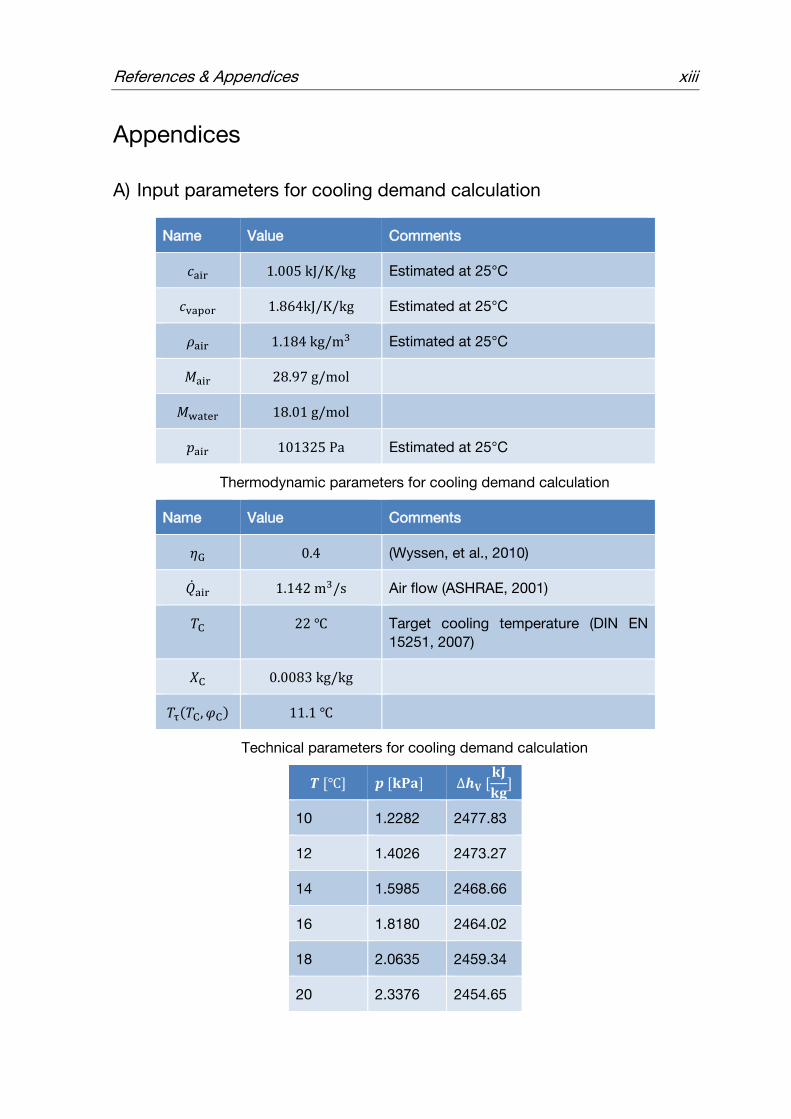
References & Appendices xiii
Appendices
A) Input parameters for cooling demand calculation
Name Value Comments
𝑐air 1.005 kJ/K/kg Estimated at 25°C
𝑐vapor 1.864kJ/K/kg Estimated at 25°C
𝜌air 1.184 kg/m3 Estimated at 25°C
𝑀air 28.97 g/mol
𝑀water 18.01 g/mol
𝑝air 101325 Pa Estimated at 25°C
Thermodynamic parameters for cooling demand calculation
Name Value Comments
𝜂G 0.4 (Wyssen, et al., 2010)
�̇�air 1.142 m3/s Air flow (ASHRAE, 2001)
𝑇C 22 ℃ Target cooling temperature (DIN EN
15251, 2007)
𝑋C 0.0083 kg/kg
𝑇τ(𝑇C, 𝜑C) 11.1 ℃
Technical parameters for cooling demand calculation
𝑻 [℃] 𝒑 [𝐤𝐏𝐚] ∆𝒉𝐕 [𝐤𝐉
𝐤𝐠]
10 1.2282 2477.83
12 1.4026 2473.27
14 1.5985 2468.66
16 1.8180 2464.02
18 2.0635 2459.34
20 2.3376 2454.65

xiv References & Appendices
22 2.6431 2449.94
24 2.9830 2445.21
26 3.3604 2440.48
28 3.7789 2435.74
30 4.2420 2431.00
32 4.7536 2426.25
34 5.3181 2421.50
36 5.9398 2416.74
38 6.6235 2411.97
40 7.3743 2407.20
Steam table for cooling demand calculation (Somerton, 2012)
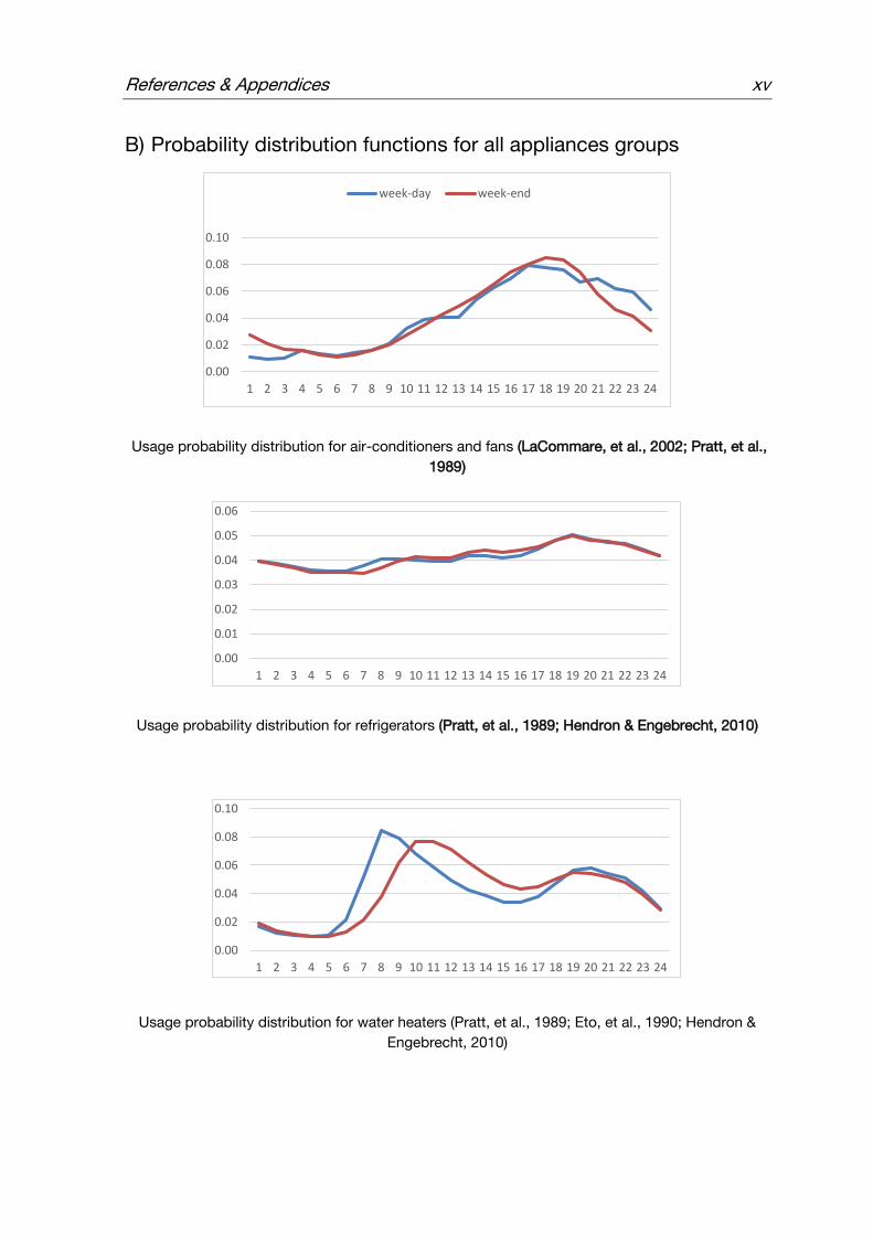
References & Appendices xv
B) Probability distribution functions for all appliances groups
Usage probability distribution for air-conditioners and fans (LaCommare, et al., 2002; Pratt, et al.,
1989)
Usage probability distribution for refrigerators (Pratt, et al., 1989; Hendron & Engebrecht, 2010)
Usage probability distribution for water heaters (Pratt, et al., 1989; Eto, et al., 1990; Hendron &
Engebrecht, 2010)
0.00
0.02
0.04
0.06
0.08
0.10
1 2 3 4 5 6 7 8 9 10 11 12 13 14 15 16 17 18 19 20 21 22 23 24
week-day week-end
0.00
0.01
0.02
0.03
0.04
0.05
0.06
1 2 3 4 5 6 7 8 9 10 11 12 13 14 15 16 17 18 19 20 21 22 23 24
0.00
0.02
0.04
0.06
0.08
0.10
1 2 3 4 5 6 7 8 9 10 11 12 13 14 15 16 17 18 19 20 21 22 23 24

xvi References & Appendices
Usage probability distribution for room heaters (Pratt, et al., 1989)
Usage probability distribution for cooking appliances (Pratt, et al., 1989; Eto, et al., 1990; Hendron
& Engebrecht, 2010)
Usage probability distribution for lighting appliances (Pratt, et al., 1989)
0.00
0.02
0.04
0.06
0.08
1 2 3 4 5 6 7 8 9 10 11 12 13 14 15 16 17 18 19 20 21 22 23 24
0.00
0.05
0.10
0.15
0.20
1 2 3 4 5 6 7 8 9 10 11 12 13 14 15 16 17 18 19 20 21 22 23 24
0.00
0.05
0.10
0.15
0.20
1 2 3 4 5 6 7 8 9 10 11 12 13 14 15 16 17 18 19 20 21 22 23 24

References & Appendices xvii
Usage probability distribution for washing and cleaning appliances (Pratt, et al., 1989; Eto, et al.,
1990; Hendron & Engebrecht, 2010)
Usage probability distribution for entertainment appliances (Pratt, et al., 1989)
Usage probability distribution for other appliances (Pratt, et al., 1989)
0.00
0.02
0.04
0.06
0.08
1 2 3 4 5 6 7 8 9 10 11 12 13 14 15 16 17 18 19 20 21 22 23 24
0.00
0.01
0.02
0.03
0.04
0.05
0.06
0.07
1 2 3 4 5 6 7 8 9 10 11 12 13 14 15 16 17 18 19 20 21 22 23 24
0.00
0.01
0.02
0.03
0.04
0.05
0.06
0.07
1 2 3 4 5 6 7 8 9 10 11 12 13 14 15 16 17 18 19 20 21 22 23 24

xviii References & Appendices
C) Data and Weibull correlations for ownership rates/electrification
rates projection
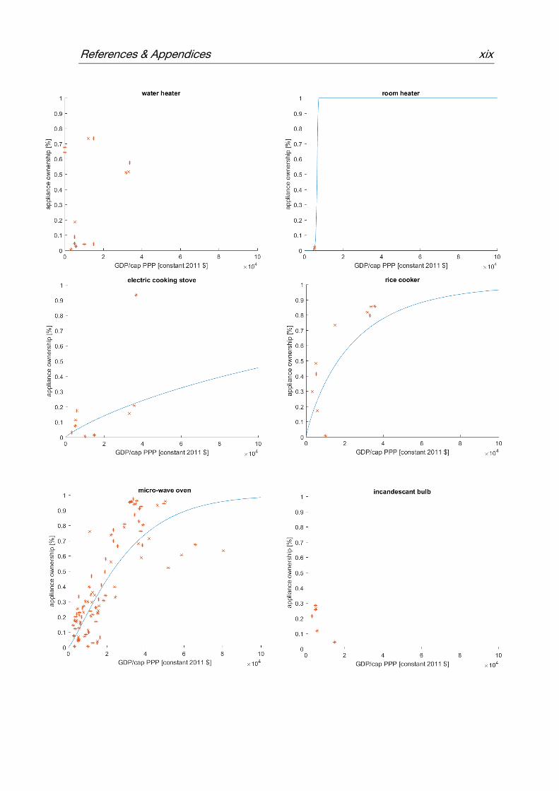
References & Appendices xix

xx References & Appendices

References & Appendices xxi

xxii References & Appendices
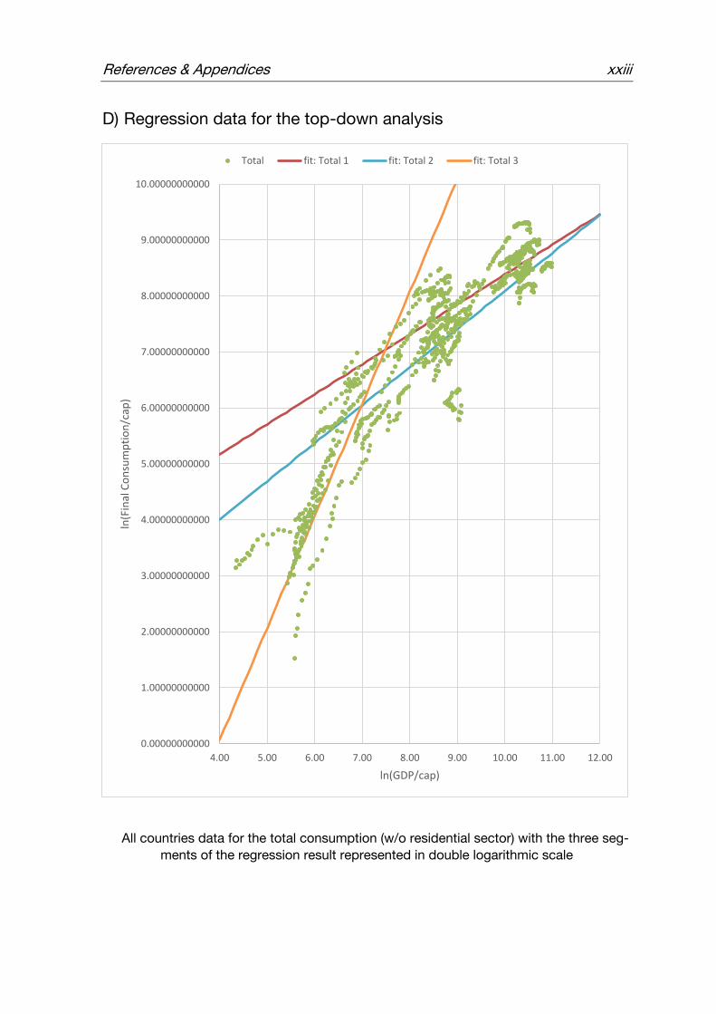
References & Appendices xxiii
D) Regression data for the top-down analysis
All countries data for the total consumption (w/o residential sector) with the three seg-
ments of the regression result represented in double logarithmic scale
0.00000000000
1.00000000000
2.00000000000
3.00000000000
4.00000000000
5.00000000000
6.00000000000
7.00000000000
8.00000000000
9.00000000000
10.00000000000
4.00 5.00 6.00 7.00 8.00 9.00 10.00 11.00 12.00
ln(F
inal
Co
nsu
mp
tio
n/c
ap)
ln(GDP/cap)
Total fit: Total 1 fit: Total 2 fit: Total 3
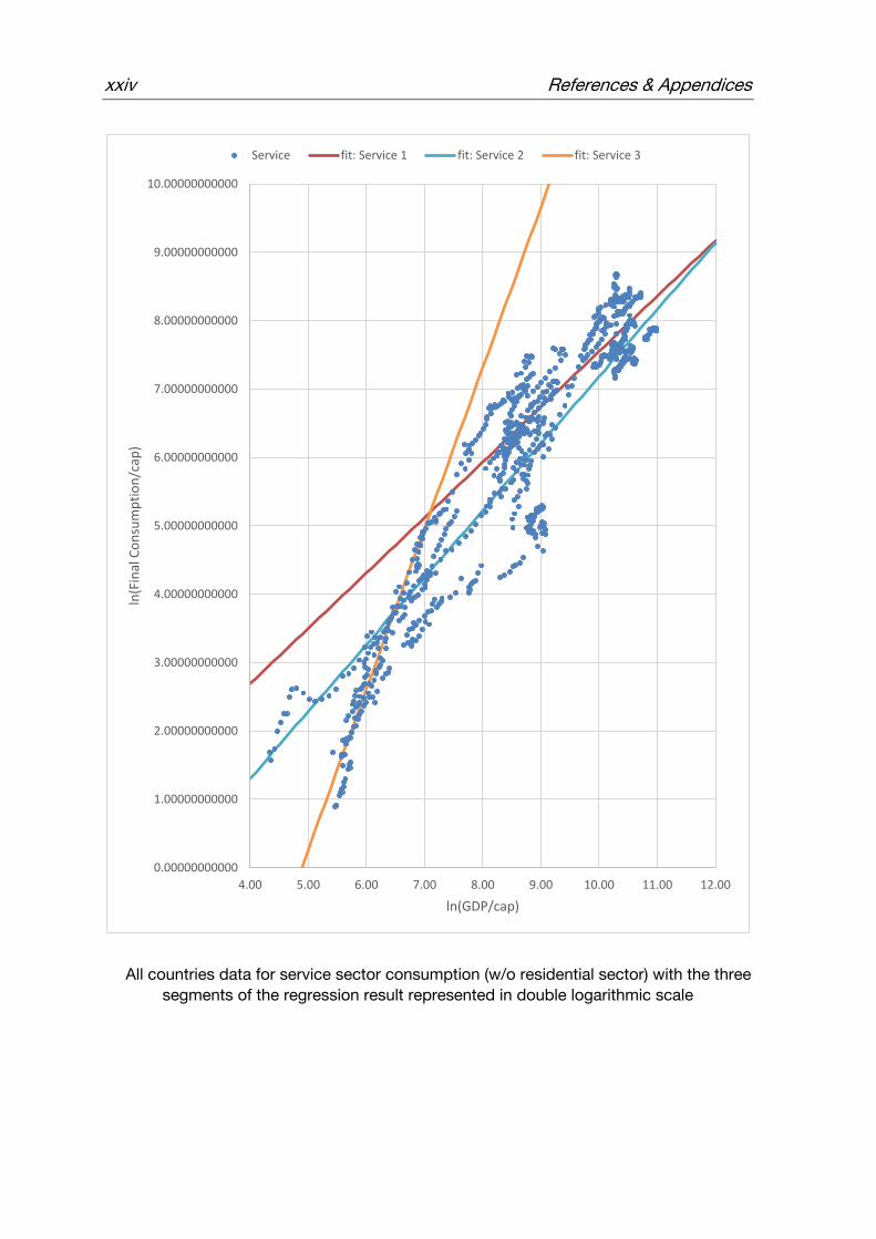
xxiv References & Appendices
All countries data for service sector consumption (w/o residential sector) with the three
segments of the regression result represented in double logarithmic scale
0.00000000000
1.00000000000
2.00000000000
3.00000000000
4.00000000000
5.00000000000
6.00000000000
7.00000000000
8.00000000000
9.00000000000
10.00000000000
4.00 5.00 6.00 7.00 8.00 9.00 10.00 11.00 12.00
ln(F
inal
Co
nsu
mp
tio
n/c
ap)
ln(GDP/cap)
Service fit: Service 1 fit: Service 2 fit: Service 3
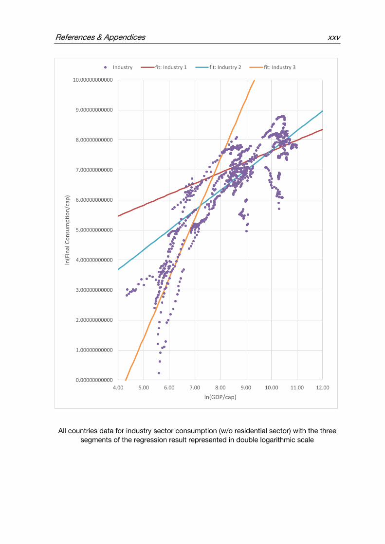
References & Appendices xxv
All countries data for industry sector consumption (w/o residential sector) with the three
segments of the regression result represented in double logarithmic scale
0.00000000000
1.00000000000
2.00000000000
3.00000000000
4.00000000000
5.00000000000
6.00000000000
7.00000000000
8.00000000000
9.00000000000
10.00000000000
4.00 5.00 6.00 7.00 8.00 9.00 10.00 11.00 12.00
ln(F
inal
Co
nsu
mp
tio
n/c
ap)
ln(GDP/cap)
Industry fit: Industry 1 fit: Industry 2 fit: Industry 3

xxvi References & Appendices
parame-ter
Cate-gory
b ln(a) a R^2 Intersec-tion
Total 1 0.5358 3.0287 20.670344 0.6042
2 0.6805 1.2865 3.620094 0.4955 169410.9892
3 2.0043 -7.9561 0.0003505 0.5843 1076.930747
Service 1 0.8085 -0.5398 0.5828648 0.6437
2 0.9801 -2.6177 0.0729705 0.634 181493.362
3 2.3487 -11.48 1.033E-05 0.7365 649.0108044
Industry 1 0.3607 4.0243 55.941136 0.2059
2 0.6614 1.033 2.8094816 0.4519 20905.9376
3 1.9894 -8.5475 0.000194 0.2979 1358.629741
Parameters derived from the regressions
Resulting power functions derived from the regressions
0.00
2,000.00
4,000.00
6,000.00
8,000.00
10,000.00
12,000.00
- 10,000.00 20,000.00 30,000.00 40,000.00 50,000.00 60,000.00
TFC
/cap
[kW
h/c
ap]
GDP/cap [constant 2005 US$]
Total consumption
all sectors service industry fit : all sectors fit: service fit: industry

References & Appendices xxvii
E) Demand estimates from top-down model (moderate scenario)
Projections for total electricity consumption per capita
0.00
1,000.00
2,000.00
3,000.00
4,000.00
5,000.00
6,000.00
7,000.00
8,000.00
9,000.00
10,000.00
- 5,000.00 10,000.00 15,000.00 20,000.00 25,000.00 30,000.00 35,000.00 40,000.00 45,000.00 50,000.00
TFC
/cap
[kW
h/c
ap]
GDP/cap [constant 2005 US$]
Total (w/o residential)
Malaysia Malaysia (projection) Singapore Singapore (projection)
Indonesia Indonesia (projection) Philippines Philippines (projection)
Brunei Brunei (projection) Thailand Thailand (projection)
Myanmar Myanmar (projection) Cambodia Cambodia (projection)
Vietnam Vietnam (projection) Laos Laos (projection)

xxviii References & Appendices
Projections for electricity consumption per capita in service sector
0.00
1,000.00
2,000.00
3,000.00
4,000.00
5,000.00
6,000.00
7,000.00
- 5,000.00 10,000.00 15,000.00 20,000.00 25,000.00 30,000.00 35,000.00 40,000.00 45,000.00 50,000.00
TFC
/cap
[kW
h/c
ap]
GDP/cap [constant 2005 US$]
Service sector
Malaysia Malaysia (projection) Singapore Singapore (projection)
Indonesia Indonesia (projection) Philippines Philippines (projection)
Brunei Brunei (projection) Thailand Thailand (projection)
Myanmar Myanmar (projection) Cambodia Cambodia (projection)
Vietnam Vietnam (projection) Laos Laos (projection)

References & Appendices xxix
Projections for electricity consumption per capita in industry sector
0.00
500.00
1,000.00
1,500.00
2,000.00
2,500.00
3,000.00
3,500.00
4,000.00
4,500.00
- 5,000.00 10,000.00 15,000.00 20,000.00 25,000.00 30,000.00 35,000.00 40,000.00 45,000.00 50,000.00
TFC
/cap
[kW
h/c
ap]
GDP/cap [constant 2005 US$]
Industry sector
Malaysia Malaysia (projection) Singapore Singapore (projection)
Indonesia Indonesia (projection) Philippines Philippines (projection)
Brunei Brunei (projection) Thailand Thailand (projection)
Myanmar Myanmar (projection) Cambodia Cambodia (projection)
Vietnam Vietnam (projection) Laos Laos (projection)

xxx References & Appendices
F) Daily total load profiles over one year from actual available data
The electricity load profile of the region is represented from data for the whole year
(EMA, 2016; Suruhanjaya Tenaga, 2013; EDL, 2015). The important observation here is
that the load shape is almost uniform over all similar days (week-day/week-end). The fluc-
tuation in magnitude for the same type of days (weekday/weekend) are due to meteoro-
logical and probabilistic effects (see sub-section 2.5.1). Moreover, the difference in mag-
nitude between weekday and weekend is clear in the data of Peninsular Malaysia (the red
and blue band) and of Singapore (green and purple band). For these two sets of data, the
highest load happens during the day (afternoon). These two characteristics are due to the
important share of the industrial and service sector in the electricity consumption (see
3.2.4). This is not the case for Laos, where weekday and weekend load are in the same
interval and the load peak occurs in the evening due to residential demand.
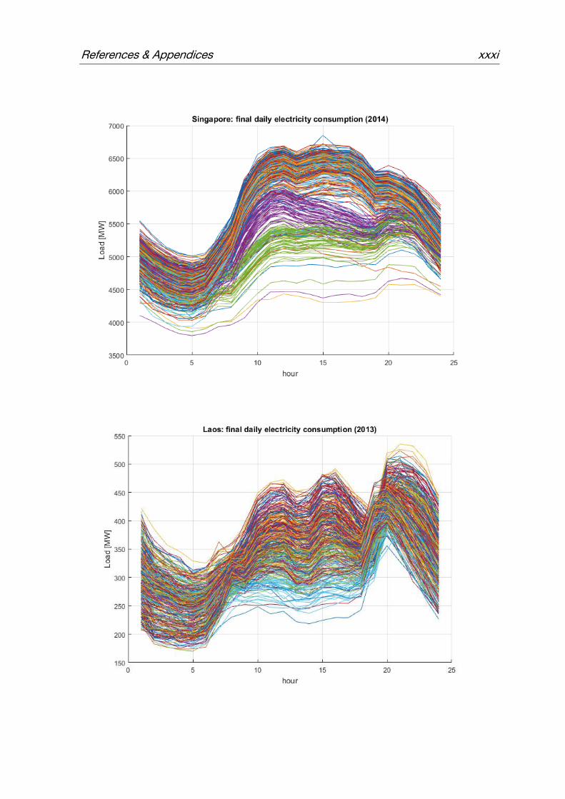
References & Appendices xxxi
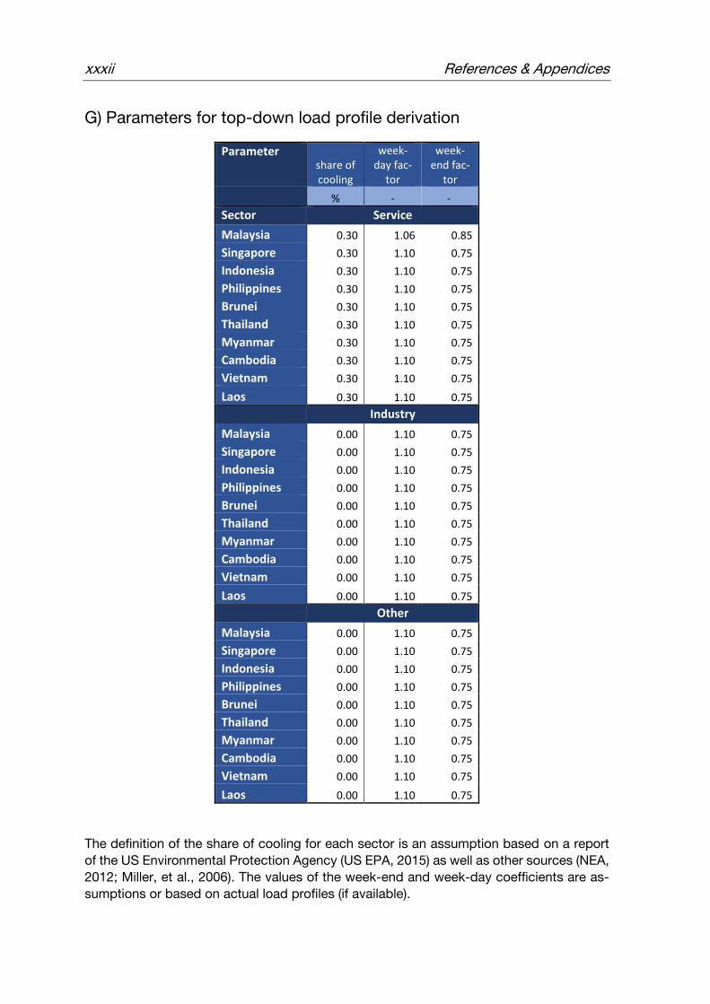
xxxii References & Appendices
G) Parameters for top-down load profile derivation
Parameter share of cooling
week-day fac-
tor
week-end fac-
tor
% - -
Sector Service
Malaysia 0.30 1.06 0.85
Singapore 0.30 1.10 0.75
Indonesia 0.30 1.10 0.75
Philippines 0.30 1.10 0.75
Brunei 0.30 1.10 0.75
Thailand 0.30 1.10 0.75
Myanmar 0.30 1.10 0.75
Cambodia 0.30 1.10 0.75
Vietnam 0.30 1.10 0.75
Laos 0.30 1.10 0.75
Industry
Malaysia 0.00 1.10 0.75
Singapore 0.00 1.10 0.75
Indonesia 0.00 1.10 0.75
Philippines 0.00 1.10 0.75
Brunei 0.00 1.10 0.75
Thailand 0.00 1.10 0.75
Myanmar 0.00 1.10 0.75
Cambodia 0.00 1.10 0.75
Vietnam 0.00 1.10 0.75
Laos 0.00 1.10 0.75
Other
Malaysia 0.00 1.10 0.75
Singapore 0.00 1.10 0.75
Indonesia 0.00 1.10 0.75
Philippines 0.00 1.10 0.75
Brunei 0.00 1.10 0.75
Thailand 0.00 1.10 0.75
Myanmar 0.00 1.10 0.75
Cambodia 0.00 1.10 0.75
Vietnam 0.00 1.10 0.75
Laos 0.00 1.10 0.75
The definition of the share of cooling for each sector is an assumption based on a report
of the US Environmental Protection Agency (US EPA, 2015) as well as other sources (NEA,
2012; Miller, et al., 2006). The values of the week-end and week-day coefficients are as-
sumptions or based on actual load profiles (if available).

References & Appendices xxxiii
H) Model final outputs compared to existing studies
The projections for the total final consumption (all sectors aggregated) in the moderate
scenario is plotted with projections from the APERC Energy Demand and Supply Outlook
(APERC, 2016) and the ADB Energy Outlook for Asia and the Pacific (ADB, 2013). The
projected values are from 2015 until 2040.
0.00
5.00
10.00
15.00
20.00
25.00
30.00
35.00
1990 1995 2000 2005 2010 2015 2020 2025 2030 2035 2040
Tota
l Fin
al C
on
sum
pti
on
[M
toe]
Malaysia
This study (moderate scenario) APEC (BAU) ADB (BAU)
0.00
1.00
2.00
3.00
4.00
5.00
6.00
7.00
1990 1995 2000 2005 2010 2015 2020 2025 2030 2035 2040
Tota
l Fin
al C
on
sum
pti
on
[M
toe]
Singapore
APEC (BAU) This study (moderate scenario) ADB (BAU)
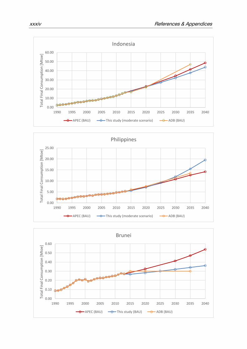
xxxiv References & Appendices
0.00
10.00
20.00
30.00
40.00
50.00
60.00
1990 1995 2000 2005 2010 2015 2020 2025 2030 2035 2040
Tota
l Fin
al C
on
sum
pti
on
[M
toe]
Indonesia
APEC (BAU) This study (moderate scenario) ADB (BAU)
0.00
5.00
10.00
15.00
20.00
25.00
1990 1995 2000 2005 2010 2015 2020 2025 2030 2035 2040
Tota
l Fin
al C
on
sum
pti
on
[M
toe]
Philippines
APEC (BAU) This study (moderate scenario) ADB (BAU)
0.00
0.10
0.20
0.30
0.40
0.50
0.60
1990 1995 2000 2005 2010 2015 2020 2025 2030 2035 2040
Tota
l Fin
al C
on
sum
pti
on
[M
toe]
Brunei
APEC (BAU) This study (BAU) ADB (BAU)

References & Appendices xxxv
0.00
5.00
10.00
15.00
20.00
25.00
30.00
35.00
1990 1995 2000 2005 2010 2015 2020 2025 2030 2035 2040
Tota
l Fin
al C
on
sum
pti
on
[M
toe]
Thailand
APEC (BAU) This study (moderate scenario) ADB (BAU)
0.00
0.50
1.00
1.50
2.00
2.50
3.00
3.50
1990 1995 2000 2005 2010 2015 2020 2025 2030 2035 2040
Tota
l Fin
al C
on
sum
pti
on
[M
toe]
Myanmar
This study (BAU) ADB (BAU)
0.00
0.20
0.40
0.60
0.80
1.00
1.20
1.40
1.60
1.80
2.00
1990 1995 2000 2005 2010 2015 2020 2025 2030 2035 2040
Tota
l Fin
al C
on
sum
pti
on
[M
toe]
Cambodia
This study (moderate scenario) ADB (BAU)
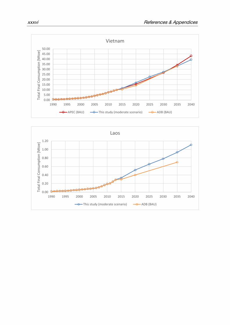
xxxvi References & Appendices
0.00
5.00
10.00
15.00
20.00
25.00
30.00
35.00
40.00
45.00
50.00
1990 1995 2000 2005 2010 2015 2020 2025 2030 2035 2040
Tota
l Fin
al C
on
sum
pti
on
[M
toe]
Vietnam
APEC (BAU) This study (moderate scenario) ADB (BAU)
0.00
0.20
0.40
0.60
0.80
1.00
1.20
1990 1995 2000 2005 2010 2015 2020 2025 2030 2035 2040
Tota
l Fin
al C
on
sum
pti
on
[M
toe]
Laos
This study (moderate scenario) ADB (BAU)

References & Appendices xxxvii
I) Demand projections according to scenarios
According to the scenarios described in 4.3, the final electricity demand projection is rep-
resented for each ASEAN country.
0.00
5.00
10.00
15.00
20.00
25.00
30.00
35.00
19
90
19
92
19
94
19
96
19
98
20
00
20
02
20
04
20
06
20
08
20
10
20
12
20
14
20
16
20
18
20
20
20
22
20
24
20
26
20
28
20
30
20
32
20
34
20
36
20
38
20
40
Tota
l dem
and
[M
toe]
Demand scenarios: Malaysia
Scenario 1 Scenario 2 Scenario 3 Historic data
0.00
1.00
2.00
3.00
4.00
5.00
6.00
7.00
19
90
19
92
19
94
19
96
19
98
20
00
20
02
20
04
20
06
20
08
20
10
20
12
20
14
20
16
20
18
20
20
20
22
20
24
20
26
20
28
20
30
20
32
20
34
20
36
20
38
20
40
Tota
l dem
and
[M
toe]
Demand scenarios: Singapore
Scenario 1 Scenario 2 Scenario 3 Historic data

xxxviii References & Appendices
0.00
10.00
20.00
30.00
40.00
50.00
60.001
99
0
19
92
19
94
19
96
19
98
20
00
20
02
20
04
20
06
20
08
20
10
20
12
20
14
20
16
20
18
20
20
20
22
20
24
20
26
20
28
20
30
20
32
20
34
20
36
20
38
20
40
Tota
l dem
and
[M
toe]
Demand scenarios: Indoensia
Scenario 1 Scenario 2 Scenario 3 Historic data
0.00
5.00
10.00
15.00
20.00
25.00
19
90
19
92
19
94
19
96
19
98
20
00
20
02
20
04
20
06
20
08
20
10
20
12
20
14
20
16
20
18
20
20
20
22
20
24
20
26
20
28
20
30
20
32
20
34
20
36
20
38
20
40
Tota
l dem
and
[M
toe]
Demand scenarios: Philippines
Scenario 1 Scenario 2 Scenario 3 Historic data
0.00
0.05
0.10
0.15
0.20
0.25
0.30
0.35
0.40
19
90
19
92
19
94
19
96
19
98
20
00
20
02
20
04
20
06
20
08
20
10
20
12
20
14
20
16
20
18
20
20
20
22
20
24
20
26
20
28
20
30
20
32
20
34
20
36
20
38
20
40
Tota
l dem
and
[M
toe]
Demand scenarios: Brunei
Scenario 1 Scenario 2 Scenario 3 Historic data
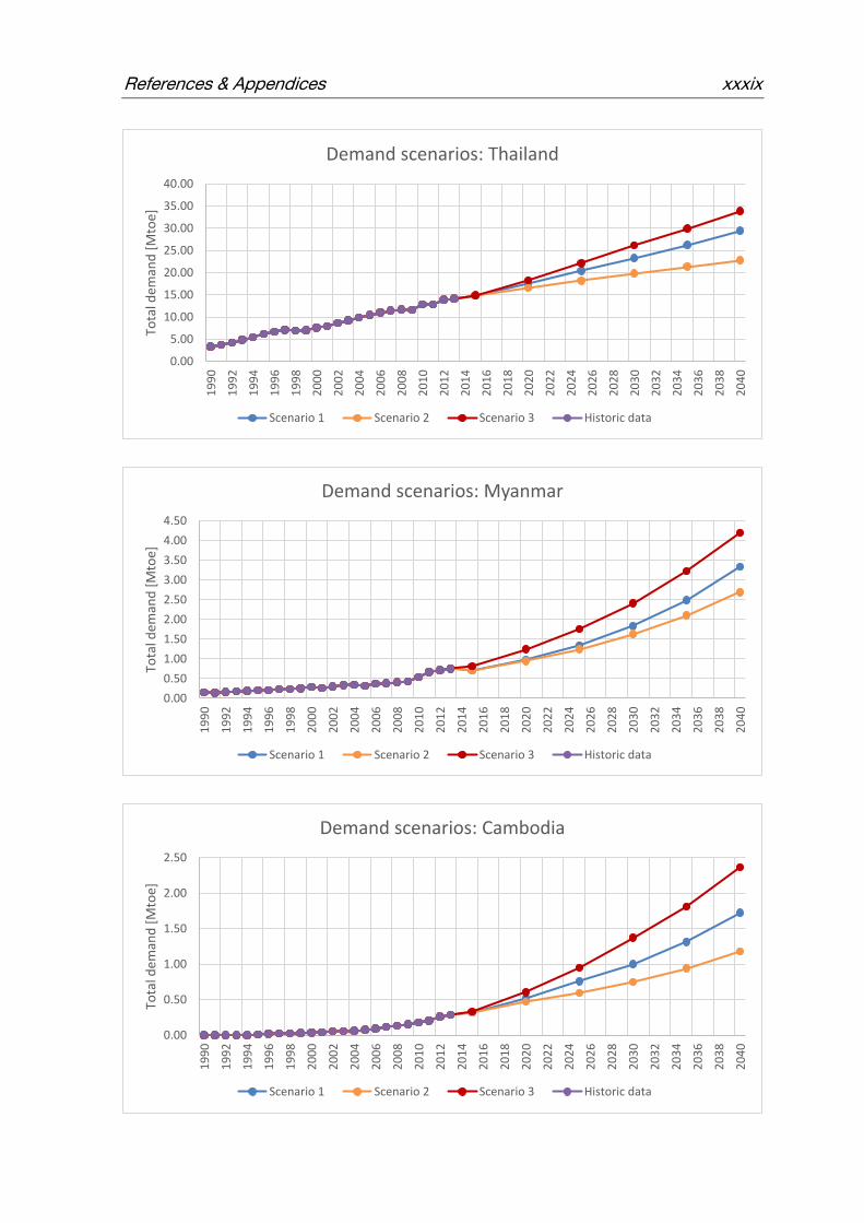
References & Appendices xxxix
0.00
5.00
10.00
15.00
20.00
25.00
30.00
35.00
40.00
19
90
19
92
19
94
19
96
19
98
20
00
20
02
20
04
20
06
20
08
20
10
20
12
20
14
20
16
20
18
20
20
20
22
20
24
20
26
20
28
20
30
20
32
20
34
20
36
20
38
20
40
Tota
l dem
and
[M
toe]
Demand scenarios: Thailand
Scenario 1 Scenario 2 Scenario 3 Historic data
0.00
0.50
1.00
1.50
2.00
2.50
3.00
3.50
4.00
4.50
19
90
19
92
19
94
19
96
19
98
20
00
20
02
20
04
20
06
20
08
20
10
20
12
20
14
20
16
20
18
20
20
20
22
20
24
20
26
20
28
20
30
20
32
20
34
20
36
20
38
20
40
Tota
l dem
and
[M
toe]
Demand scenarios: Myanmar
Scenario 1 Scenario 2 Scenario 3 Historic data
0.00
0.50
1.00
1.50
2.00
2.50
19
90
19
92
19
94
19
96
19
98
20
00
20
02
20
04
20
06
20
08
20
10
20
12
20
14
20
16
20
18
20
20
20
22
20
24
20
26
20
28
20
30
20
32
20
34
20
36
20
38
20
40
Tota
l dem
and
[M
toe]
Demand scenarios: Cambodia
Scenario 1 Scenario 2 Scenario 3 Historic data

xl References & Appendices
0.00
5.00
10.00
15.00
20.00
25.00
30.00
35.00
40.00
45.00
50.001
99
0
19
92
19
94
19
96
19
98
20
00
20
02
20
04
20
06
20
08
20
10
20
12
20
14
20
16
20
18
20
20
20
22
20
24
20
26
20
28
20
30
20
32
20
34
20
36
20
38
20
40
Tota
l dem
and
[M
toe]
Demand scenarios: Vietnam
Scenario 1 Scenario 2 Scenario 3 Historic data
0.00
0.20
0.40
0.60
0.80
1.00
1.20
1.40
19
90
19
92
19
94
19
96
19
98
20
00
20
02
20
04
20
06
20
08
20
10
20
12
20
14
20
16
20
18
20
20
20
22
20
24
20
26
20
28
20
30
20
32
20
34
20
36
20
38
20
40
Tota
l dem
and
[M
toe]
Demand scenarios: Laos
Scenario 1 Scenario 2 Scenario 3 Historic data


