Page 1
ELECTRICITY DEMAND PREDICTION USING ARTIFICIAL NEURAL NETWORK
FRAMEWORK
A Paper
Submitted to the Graduate Faculty
of the
North Dakota State University
of Agriculture and Applied Science
By
Sowjanya Param
In Partial Fulfillment of the Requirements
for the Degree of
MASTER OF SCIENCE
Major Department:
Computer Science
June 2015
Fargo, North Dakota
Page 2
North Dakota State University
Graduate School
Title
ELECTRICITY DEMAND PREDICTION USING ARTIFICIAL NEURAL
NETWORK FRAMEWORK
By
SOWJANYA PARAM
The Supervisory Committee certifies that this disquisition complies with North Dakota State
University’s regulations and meets the accepted standards for the degree of
MASTER OF SCIENCE
SUPERVISORY COMMITTEE:
Dr. Kendall Nygard
Chair
Dr. Simone Ludwig
Dr. Jacob Glower
Approved:
06/09/2015 Dr.Brian Slator
Date Department Chair
Page 3
iii
ABSTRACT
As the economy is growing, electricity usage has been growing and to meet the needs of
energy market in providing the electricity without power outages, utility companies, distributors
and investors need a powerful tool that can effectively predict electricity demand day ahead that
can help them in making better decisions in inventory planning, power generation, and resource
management. Historical data is a great source that can be used with artificial neural networks to
predict electricity demand effectively with a decent error rate of 0.06.
Page 4
iv
ACKNOWLEDGEMENTS
I would like to express my sincere thanks to my advisor Dr. Kendall Nygard for his
continued support throughout this paper. I am grateful to the ideas and suggestions given by Dr.
Nygard, and the amount of guidance given by him is enormous. Also special thanks go to my
advisory committee members for their inputs and valuable suggestions that helped me complete
this paper.
I thank all my graduate faculty members for sharing their knowledge and experience with
me. I would like to thank Ms. Carole, Ms. Stephanie and Ms. Betty personally and the entire
computer science department staff members for their enormous support.
Many Thanks to Zoran Severac and developers of Neuroph for building a great neural
network framework, which is used in this project.
Finally, words alone cannot express the thanks I owe to my husband, dad, mom and sister
for their support and thanks to Levi Strauss & Co, San Francisco colleagues for all their support.
Once again I am very thankful to my advisor Dr.Nygard for his valuable suggestions and
support that helped me to complete this paper successfully.
Page 5
v
TABLE OF CONTENTS
ABSTRACT ................................................................................................................................... iii
ACKNOWLEDGEMENTS ........................................................................................................... iv
LIST OF TABLES ....................................................................................................................... viii
LIST OF FIGURES ....................................................................................................................... ix
CHAPTER 1. INTRODUCTION ................................................................................................... 1
CHAPTER 2. LITERATURE REVIEW ........................................................................................ 4
2.1. Electricity demand prediction using artificial neural networks ........................................... 4
2.2. Why use neural network frameworks? ................................................................................. 5
2.3. Why use Neuroph? ............................................................................................................... 6
CHAPTER 3. INTRODUCTION TO NEUROPH ......................................................................... 8
3.1. Neuroph framework ............................................................................................................. 8
3.1.1. Neuroph Library ............................................................................................................ 9
3.1.2. Neuroph Studio .............................................................................................................. 9
3.2. Overview of neural networks with Neuroph Studio............................................................. 9
3.3. Neuroph Studio with an example AND gate ...................................................................... 12
3.3.1. Installation ................................................................................................................... 12
3.3.2 Executing AND gate ..................................................................................................... 12
CHAPTER 4. ELECTRICITY MARKET .................................................................................... 20
4.1. Electricity market in USA .................................................................................................. 20
Page 6
vi
4.2. Electricity demand data ...................................................................................................... 22
CHAPTER 5. DEMAND PREDICTION ..................................................................................... 24
5.1. Multilayer perceptron ......................................................................................................... 24
5.2. Hidden layers and neurons ................................................................................................. 26
5.3. Training method ................................................................................................................. 27
5.4. Preprocessing input data .................................................................................................... 29
5.4.1. Flattening data ............................................................................................................. 30
5.4.2. Average calculator ....................................................................................................... 31
5.4.3. Normalization .............................................................................................................. 32
CHAPTER 6. ELECTRICITY DEMAND PREDICTION WITH NEUROPH ........................... 33
6.1. Software simulation............................................................................................................ 33
6.2. Analysis on the training attempts ....................................................................................... 37
6.3. Cross-validation ................................................................................................................. 41
6.4. Analysis with Linear Regression........................................................................................ 44
CHAPTER 7. ELECTRICITY DEMAND PREDICTION ON WEB.......................................... 47
7.1. Create MLP neural network ............................................................................................... 47
7.2. Upload datasets .................................................................................................................. 48
7.3. Train neural network .......................................................................................................... 49
7.4. Test neural network ............................................................................................................ 51
7.5. Cross-validate neural network ............................................................................................ 53
Page 7
vii
7.6. Predict demand ................................................................................................................... 55
CHAPTER 8. CONCLUSION AND FUTURE WORK .............................................................. 58
REFERENCES ............................................................................................................................. 59
Page 8
viii
LIST OF TABLES
Table Page
1: Analysis of neural network architecture with varying learning rate, momentum, hidden
neurons for Dataset 2009-2014 .......................................................................................... 38
2: Cross-validation with twelve sets of test data .................................................................... 42
3: Forecast with Neuroph vs real time demand. ..................................................................... 43
4: Comparision of forecast with artificial neural network output vs real time demand ......... 44
5: Analysis of forecast with artificial neural network output vs real time demand vs Linear
Regression. ......................................................................................................................... 46
Page 9
ix
LIST OF FIGURES
Figure Page
1: Neuroph framework .............................................................................................................. 8
2: New project for basic neuron sample ................................................................................. 11
3: Basic neuron sample ........................................................................................................... 11
4: Installing Neuroph Studio ................................................................................................... 12
5: Creating a new project ........................................................................................................ 13
6: Creating a new project in Neuroph Studio.......................................................................... 13
7: AND gate implementation using Neuroph ......................................................................... 14
8: Last step of creating a new project ..................................................................................... 14
9: Selecting type of neural network in Neuroph ..................................................................... 15
10: Selecting input and output neurons ................................................................................... 15
11: AND gate project with inputs and output neurons ........................................................... 16
12: Training the AND gate ..................................................................................................... 16
13: Inputting the values to the AND gate as part of training .................................................. 17
14: Trainig the neural network ................................................................................................ 17
15: Setting up learning parameters ......................................................................................... 18
16: Network error graph.......................................................................................................... 18
17: Testing the AND gate neural network project with inputs ............................................... 19
18: Electricity sales and power sector generating capacity, Source:EIA ................................ 21
Page 10
x
19: Feed forward neural network example diagram ............................................................... 24
20: Java class for multilayer perceptron in Neuroph .............................................................. 25
21: Back propagation training method .................................................................................... 27
22: Java code for creating a neural network in Neuroph ........................................................ 28
23: Java code for testing a neural network in Neuroph .......................................................... 29
24: Shell script for flattening data ........................................................................................... 30
25: Shell script for average calculator .................................................................................... 31
26: Normalization step with min max formula ....................................................................... 32
27: Setting up Neuroph for the Electricity Demand forecasting project ................................ 33
28: Unzipping the Neuroph Studio ......................................................................................... 33
29: Successfully installed Neuroph studio .............................................................................. 34
30: Navigate to EDP project ................................................................................................... 34
31: Setting up the learning parameters for electricity demand forecasting ............................ 35
32: Network error graph.......................................................................................................... 36
33: Testing the trained neural network ................................................................................... 36
34: Output after training and testing ....................................................................................... 37
35: Test results from the best neural network architecture with 56 neurons .......................... 40
36: Total network error graph after successfully training and testing the neural network ..... 41
37: Neural network architecture with 56 hidden neurons ....................................................... 41
Page 11
xi
38: Linear Regression for average demand with real time demand ........................................ 45
39: Creating a multilayer perceptron neural network ............................................................. 47
40: Java code for creating a neural network ........................................................................... 48
41: Uploading training set ....................................................................................................... 48
42: Java code for uploading training set ................................................................................. 49
43: Training a neural network ................................................................................................. 49
44: Java code for training a neural network ............................................................................ 50
45: Training logs generated from a neural network during the training phase ....................... 51
46: Testing a neural network ................................................................................................... 52
47: Java code for testing a neural network.............................................................................. 53
48: Cross-validating a neural network .................................................................................... 54
49: Java code for cross-validation........................................................................................... 54
50: Predicting electricity demand ........................................................................................... 55
51: Output of electricity demand after it’s predicted .............................................................. 56
52: Java code for electricity demand prediction ..................................................................... 57
Page 12
1
CHAPTER 1. INTRODUCTION
Predicting electricity demand plays an important role in energy market and it affects all
the participants in the market such as Consumers, producers, investors, distributors and
regulators. Inaccurate forecasts can lead to severe losses for investors due to their bad decisions
(Küçükdeniz, 2010)and Consumers might have to end up paying more to suffer the power
outages. Producers might have to face challenges in storing the electricity in case of over
production and to build new power plants to supply the needed electricity without any outages
that might take huge amounts of resources and time in case of under production. Inability to store
large amounts of electricity in a cost effective way is one of the most important factors that
encourages the concept of forecasting.
As the electricity market is growing rapidly, there is need for tools that can learn and
predict the electricity demand accurately that can be useful to both consumers to maximize their
utilities and help power producers to maximize their profits and to minimize the financial risk by
not misjudging the price movements (J.P.S. Catalao, 2006).
Neuroph is one such framework that can solve Artificial Intelligence problems in a single
environment like pre-processing the given data by applying sigmoid functions along with the
actual/original problem solving architecture and algorithms. It is an open source framework that
gives the freedom to users to customize the library as per the problem requirements and widely
supported as the development versions are constantly releasing with new features/added
functionalities and support to various algorithms.
The objective of this paper is to predict electricity demand using one of the neural
network frameworks – Neuroph with the historical data. Using Neuroph, we create neural
network architecture and feed the Historical data in the form of training and testing sets. The
Page 13
2
training phase helps the neural network to learn from the input data and the testing phase helps in
determining the best neural network architecture by calculating the total mean square error of the
neural network and we can achieve this by varying the parameters such as momentum, hidden
neurons, learning rate and error. Then we do cross validation by using leave one out technique to
find out the standard deviation and variance of that best network and then predict the electricity
demand for future.
Different prediction methods have been applied to predict electricity by making use of
historical data such as historical averaging models such as NYISO in which the next day
prediction is calculated by taking the hourly average of the five most recent days with the highest
average load. In this paper, we build a neural network architecture and train the network by
calculating the hourly average demand for the previous years’ same day along with the demand
of the seven most recent days.
Neural network architecture is built using Neuroph and so it is important to understand
this framework, as it is helpful for many such research projects, experiments. Also, due to its
applications, central Washington university has included this as part of their coursework so that
students can take advantage to .
Understand and solve the problems in a more practical way.
Try and approach to solve a problem using different algorithms in multiple ways.
Customize the neural network library based on the problem space.
Ex: forecasting number of applicants for ndsu during this summer/fall to accommodate
the needs of the prospective students, finding the number of passengers travelling in a train
during a particular time to accommodate all passengers in a train without any problems, etc.
Page 14
3
The structure of this paper is as follows. Chapter 2 describes the related literature in
prediction and neural network frameworks. In chapter 3, the electricity market, the current trends
of consumption, source of data for this project are explained. In chapter 4, applying multilayer
perceptron with back propagation training method, normalization steps are described. This paper
will cover more details on Electricity demand and it’s importance on how it’s affecting economic
growth, Neuroph and its applications, Demand forecasting using Neuroph that includes software
simulation and Analysis of the results.
Page 15
4
CHAPTER 2. LITERATURE REVIEW
2.1. Electricity demand prediction using artificial neural networks
Predicting Electricity demand plays an important role in Inventory planning and
management, it can be achieved by an accurate prediction model. Also it helps in better
management of resources for the utility companies or distributors or investors and so it has to be
aimed first (Mitrea, Lee, & Wu, 2009).
Previous research shows that neural networks have been successfully used for many types
of forecasting problems (Smith & Gupta, 2002) and in different fields such as in financial
applications (hoseinzade & Akhavan Niaki, 2013); (Angelini, di Tollo, & Roli, 2008); (Kumar &
Walia, 2006), psychology (Levine, 2006); (Quek & Moskowitz, 2007), medicine (Lisboa &
Taktak, 2006), mathematics (Hernandez & Salinas, 2004), engineering (Pierre, Said, & Probst,
2001), tourism (Palmer, Montano, & Sese, 2006)and energy sector ( (Rodrigues, Cardeira, &
Calado, 2014); (Kargar & charsoghi, 2014); (Pankilb, Prakasvudhisarn, & Khummongkol,
2015); (Limanond, Jomnokwao, & Srikaew, 2011), (AbuAl-Foul, 2012).
(Kandananond, 2011) Did a comparative study on performance of the three approaches
such as ARIMA, ANN and MLR and found that artificial neural networks using Multilayer
perceptrons method for predicting electricity demand was superior to other approaches in terms
of error measurement. In the same lines, (Mitrea, Lee, & Wu, 2009) did a case study by
comparing Neural Networks with Traditional forecasting methods and results showed that
forecasting with Neural networks offers better performance. According to (Bacha & Meyer,
1992), it is mentioned that NN approach is able to provide a more accurate prediction than expert
systems or statistical counterpart.
Page 16
5
As per the above examples, when compared to the other traditional methods like
statistical models or time series methods, we knew that ANN is a clear winner and (Patuwo,
Zhang, & Hu, 1997) in one of his research papers mentioned the below reasons on why/how
ANN is a better method for forecasting:
ANN’s are data driven self-adaptive methods, which means that they learn from
examples and capture subtle functional relationships among the data even if the
underlying relationships are unknown or hard to describe. Thus ANNs are well suited for
problems whose solutions require knowledge that is difficult to specify but for which
there are enough data or observations (Patuwo, Zhang, & Hu, 1997).
ANN’s can generalize, even after learning the data presented to them, ANNs can often
correctly infer the unseen part of a population even if the sample data contain noisy
information (Patuwo, Zhang, & Hu, 1997).
ANN’s are universal functional approximators as they have more general and flexible
functional forms than the traditional statistical methods can effectively deal with due to
the limitations in estimating the underlying function due to the complexity of the real
system (Patuwo, Zhang, & Hu, 1997).
Finally, ANNs are nonlinear which are best suitable for real world problems as they are
often non linear (Granger & Terasvirta, 1993). ANN’s are generally non-linear data
driven approaches as opposed to model-based non-linear model, which makes it much
better for forecasting (Patuwo, Zhang, & Hu, 1997).
2.2. Why use neural network frameworks?
Since ANN’s are so popular and accurate, very recently researchers have started building
a collaborative workspace to bring the most common and widely used algorithms into a
Page 17
6
framework so that it can help other developers in easily building the desired neural network
architecture and there by encouraging them to extend a framework which is ready to use, by
providing out of the box functionality, flexible and fun to practice a problem in multiple ways.
These frameworks not only carry the same functionality which the individual ANN
algorithms might offer but also support and save time & effort of the developers in building an
efficient software which can be used for any type of problem.
Neural network frameworks such as NEUROPH, ENCOG, FANN, JOONE came into
existence and helped in solving real world problems such as stock market predictions (Heaton,
Basic market forecasting with encog neural networks, 2010), recognition of braille alphabet
(Risteski) , face recognition (Stojilkovic), predicting poker hands (Ivanić), predicting the class
of breast cancer (Trisic), lenses classification (Urosevic), blood transfusion service center
(Jovanovic A. ), predicting the result of football match (Radovanović & Radojičić), glass
identification (Čutović), wine classification (Stojković), predicting survival of patients
(Jovanovic M. ) , Music classification by genre (Jeremic) are some examples.
2.3. Why use Neuroph?
Research projects using neural network frameworks have been extensively done in the
fields such as medicine, sports, social causes but there is no such experiment that has been done
in energy sector, which inspired to take up this experiment.
According to a latest article on codeproject by (Taheri, 2010) on benchmarking and
comparing the Encog, Neuroph and JOONE frameworks, it is mentioned that the way Neuroph is
built is easier to understand when compared to encog and the lack of support of JOONE and the
complexity of their interface leaves us with the only option of Neuroph.
Page 18
7
Neuroph is a framework that simplifies the evolution of applications. It has been already
in use in the research field such as test effort estimation (JayaKumar & Alain, 2013),
Autonomous Neural Development and pruning (A.C.Andersen, 2010), FIVE-Framework for
Integrated Voice Environment (Alexandre & Edson, 2010), Efficient name disambiguation in
digital libraries (Haixun, Shijun, Satoshi , Xiaohua, & Tieyun, 2011) and also for developing
games such as backgammon etc.
In addition to the above applications, Neuroph Framework has the below advantages
Free open source neural network framework, which has built-in multilayer perceptron
network along with the training method of back propagation with momentum that gives
us the ability to use the existing framework rather than creating a new network from the
scratch.
Gives us the flexibility to add/manipulate the existing code that can be easily extended
for specific purpose with high level of reusability.
Easy to use as it has an intuitive GUI built with Netbeans.
Well documented and well supported.
Constantly rolling out with Latest versions/updates.
Hence the aim of this paper is to use Neuroph to predict electricity demand.
Some of the Previous Research indicates that the inputs of neural network not only
contain historical data but also economic conditions such as GDP, population and weather
conditions but our paper mainly focuses on predicting electricity demand based on historical data
and so Historical data along with the preprocessing is an important step which is explained in
chapter 4.
Page 19
8
CHAPTER 3. INTRODUCTION TO NEUROPH
3.1. Neuroph framework
Neuroph is a lightweight Java Neural Network Framework for developing common
neural network architectures. It contains well-designed, open source Java library with Small
number of basic classes that correspond to basic NN concepts, and GUI editor makes it easy to
learn and use. Neuroph has been fully developed and coded in Java. It is an open source project
hosted at SourceForge, and the latest version 2.9 has been released under the Apache 2.0
License. Previous versions were licensed under LGPL.
Neuroph is written in Java language and it is made up of two blocks mainly as indicated
in the diagram below
Neuroph Library
Neuroph Studio
Figure 1: Neuroph framework
Page 20
9
3.1.1. Neuroph Library
Neuroph Library is a Java Neural network library that consists of several Java packages,
giving developers both ready-made pieces of functionality and create custom additional
components which are not related to neural network architectures or learning algorithms by using
plugins.
Three of the important packages in Neuroph Library are org.neuroph.core,
org.neuroph.nnet and org.neuroph.util. The org.neuroph.core provides base classes such as data
manipulation methods, learning event systems and basic building components for neural
networks such as neural network learning algorithms, learning rules, transfer functions. The
Org.neuroph.nnet provides out-of-the-box neural networks such as network models, layer types,
neuron types, and learning algorithms. The Org.neuroph.util provides utility classes for creating
neural networks, type codes, parsing vectors, randomization and normalization techniques etc
3.1.2. Neuroph Studio
Neuroph studio is a GUI tool, built on top of the Netbeans platform and Neuroph library
which provides an easy-to-use neural network wizards and tools so that developers can create,
test and deploy various java components based on the neural networks on the same environment
which was not the case earlier as it had separate application for Java development and another
application for building/creating Neural Networks.
3.2. Overview of neural networks with Neuroph Studio
Neural networks are computational models inspired by the way the human brain works.
Although they are very simplified models based on known principles about how the brain works,
they exhibit some very interesting features, such as learning, generalization, and association
capabilities. In addition, they are good at dealing with noisy or incomplete data (Severac, 2011).
Page 21
10
Neural networks are graph-like structures that consist of a set of interconnected nodes
called neurons. Each neuron has inputs through which it receives input from other neurons
(connected to its inputs) and outputs through which it sends output to other neurons (connected
to its outputs). The way in which the neurons are interconnected determines the type of neural
network architecture (Severac, 2011).
In addition to the connection pattern among neurons, network behavior is determined by
the processing inside the neurons and so-called connection weights. Connection weights are
numerical values associated with connections among neurons, and by tweaking these values
using an appropriate algorithm (called a learning rule), we can adjust the network behavior.
Typical neuron processing includes calculating the weighted sum of neuron inputs and
connection weights and then feeding that value into some function (step, sigmoid, or tanh
functions are commonly used). The output of that function represents the output of the neuron
(Severac, 2011).
The Neuroph framework provides all of these neural network components out of the box,
regardless of whether you want to create a common type of neural network or a custom neural
network. Neuroph Studio also provides samples that demonstrate the basic principles behind
neural networks (Severac, 2011). Below is the illustration of Basic Neuron Sample
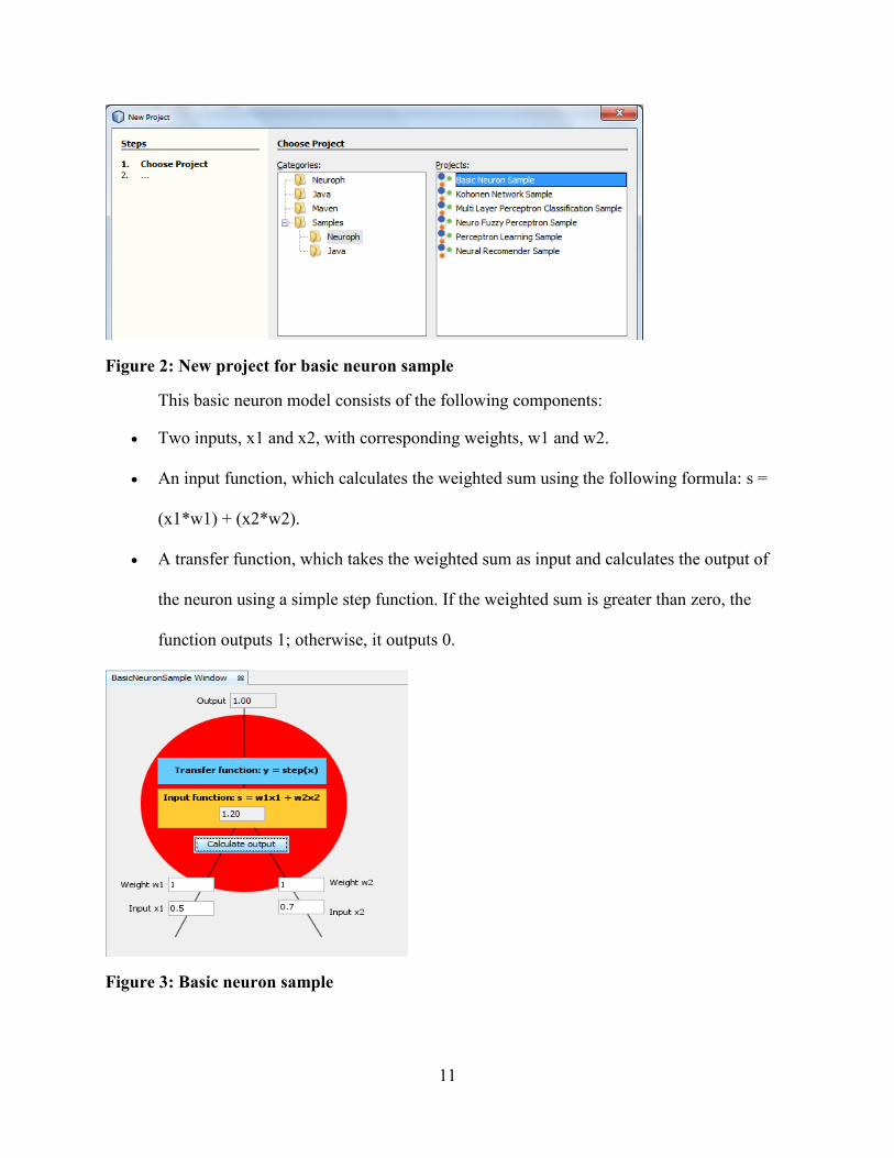
To open the basic neuron sample, in Neuroph Studio, select File >New Project > Samples
> Neuroph > Basic Neuron Sample.
Page 22
11
Figure 2: New project for basic neuron sample
This basic neuron model consists of the following components:
Two inputs, x1 and x2, with corresponding weights, w1 and w2.
An input function, which calculates the weighted sum using the following formula: s =
(x1*w1) + (x2*w2).
A transfer function, which takes the weighted sum as input and calculates the output of
the neuron using a simple step function. If the weighted sum is greater than zero, the
function outputs 1; otherwise, it outputs 0.
Figure 3: Basic neuron sample
Page 23
12
Try to run this sample and play with the neuron by changing the input and weight values,
and then click the Calculate output button.
During a learning procedure, a neuron's weights are automatically adjusted in order to get
the desired behavior. These are the basic principles of how artificial neurons work, but there are
many variations depending on the type of neural network and we can know more about the multi
layer perceptron in the chapter 4.
3.3. Neuroph Studio with an example AND gate
3.3.1. Installation
Unzip the neurophstudio package into a folder. Inside the bin directory you find 3 files
as below. For windows click on neurophstudio.exe or neurophstudio64.exe (if your OS is 64 bit)
and follow the wizard to complete installation. Launch the application from the installed
location. For MAC/Linux you can launch the application directly executing neurophstudio.sh.
Figure 4: Installing Neuroph Studio
3.3.2 Executing AND gate
Lets build a sample neural network application using Neuroph studio. For simplicity we
will take AND gate as an example and build our neural network.Click on File ->New Project
Page 24
13
Figure 5: Creating a new project
Select Neuroph -> Neuroph Project
Figure 6: Creating a new project in Neuroph Studio
Name your project as ANDGate and Click Finish
Page 25
14
Figure 7: AND gate implementation using Neuroph
You can see your project created as below
Figure 8: Last step of creating a new project
Now right click on Neural Networks folder and select New -> Neural Network. Name
your neural network as AND and select Perceptron as the type and click Next.
Page 26
15
Figure 9: Selecting type of neural network in Neuroph
In the input num field, enter 2 and in the output num field enter 1, Select Perceptron
Learning as the Learning rule and click Finish.
Figure 10: Selecting input and output neurons
Page 27
16
Your neural network created will look like below.
Figure 11: AND gate project with inputs and output neurons
Now right click on Training Sets and select new Training Set. Enter Training set name as
ANDTrainSet, Type as Supervised, Number of inputs as 2 and Number of outputs as 1.Clicknext
Figure 12: Training the AND gate
enter the training set as below and click finish
Page 28
17
Figure 13: Inputting the values to the AND gate as part of training
Now click on the neural network AND and select ANDTrainSet and click Train
Figure 14: Trainig the neural network
Set the learning parameters as below and click train.
Page 29
18
Figure 15: Setting up learning parameters
Figure 16: Network error graph
Now Click on Test and you will see the result as below
Page 30
19
Figure 17: Testing the AND gate neural network project with inputs
Page 31
20
CHAPTER 4. ELECTRICITY MARKET
According to National grid, Electricity Demand is the rate of using Electricity (National
Grid) measured in KiloWatts and the amount of energy used is called consumption. Simply put,
Demand is the rate of consumption. Both Consumption and Demand put together the electricity
consumer’s service bill. Residential consumers pay for both consumption and Demand as one as
there is relatively little variation in electricity when compared to Industrial and commercial
users.
4.1. Electricity market in USA
As per one of the documents prepared for US Department of Energy by an agency, it is
stated that Since 1982, growth in peak demand for electricity is driven by population growth,
bigger houses, bigger TV’s , more air conditioners and more computers has exceeded
transmission growth by 25% every year which is not proportional to the amount that is being
spent on R&D in this field causing delay in the advancements of this industry.
The economic consequences of an electricity shortage may be severe. (Castro &
Cramton, 2009) . As we track our history, it has been noted that in the year 2000, one hour
outage in Chicago Board of Trade resulted in 20 Trillion in trades delayed, black out in northeast
of 2003 caused $6 billion of economic loss to the region, one minute of blackout costs $1 million
to sun microsystems. These are some of the very few examples on how electricity is impacting
our economic conditions. (U.S. Department of Energy, 2007).
As the Economy is relentlessly growing towards digital, Electricity plays an important
role. Back in 1980, electrical load from the electronic equipment such as chips and automated
manufacturing was limited. By 1990, chips share grew by 10%, which is expected to rise to 60%
by 2015 (U.S. Department of Energy, 2007).
Page 32
21
According to a very recent report from (EIA), growth in electricity generating capacity
parallels the growth in end-use demand for electricity which is a good sign to prevent black outs
from happening and helps in keeping our economy stronger. So, there is a need to maintain that
corresponding relationship (the balance) between the generating capacity and the electricity
demand, which can be achieved by forecasting or predicting (the electricity demand). Hence,
Forecasting electricity is an essential step of resource planning in electricity markets to assure
that there will be sufficient resources to meet future demand as building capacity is costly and
takes time (Castro & Cramton, 2009).
Figure 18: Electricity sales and power sector generating capacity, Source:EIA
Benefits of predicting Electricity Demand include
Better resource planning in power distribution companies (Prasad, 2008) and optimize
power systems.
Reduce risks such as blackouts or power outages to the consumers,
Reduce losses/costs incurred due to the over/under production of electricity to the utility
companies.
Page 33
22
4.2. Electricity demand data
New England ISO (http://www.iso-ne.com/) is an independent, non-profit Regional
transmission organization (RTO) serving Connecticut, Maine, New Hampshire, Vermont, Rhode
Island and Massachusetts. Three critical roles of ISO-NE include
1. Operating the power system – monitor, dispatch and direct the flow of electricity across
the power grid 24 hours a day 365 days.
2. Designing, administering, and overseeing the region’s competitive wholesale electricity
markets for buying and selling day-to-day.
3. Managing the regional power system planning process - identify appropriate transmission
infrastructure solutions that are essential for maintaining power system reliability.
ISO –NE express (http://www.iso-ne.com/markets-operations/iso-express) is a great
source for both Real time and historic data in Energy, Load and Demand with parameters such as
Day Ahead Demand, Real time Demand, Load Forecast, threshold prices, bids, day-ahead and
real-time locational marginal prices (LMPs).
As the project is focused on forecasting real time demand, we have taken Real Time
Hourly Data
Real Time Hourly Data: It is the real time demand data collected per 1 hour for all the 24 hours
across a region selected or whole of the New England and is represented in MWH.
In this project, we are using the data sets ranging from January 2008 till current (2015).
Data can be downloaded for various data ranges by specifying the start and end date in the URL
(http://www.iso-ne.com/transform/csv/hourlysystemdemand?start=20140101&end=20140131)
as start=20140101&end=20140131 for the month of January for Real Time Demand Market
Page 34
23
Hourly Demand. The data set extracted from ISO-NE express site is generally a .csv file, which
consists of 3 parameters Date, Hour Ending (HE) and Real Time Demand (MWh).
Page 35
24
CHAPTER 5. DEMAND PREDICTION
Predicting Electricity Demand is an essential step to the distribution utility companies,
Power Producers and financial traders and the demand is generally predicted based on the
historical data. This project applies the concept of Multilayer perceptron with back propagation
algorithm for forecasting the demand of electricity in Neuroph framework. For the analysis
purpose, Demand data published on the ISO-NE express website is used.
5.1. Multilayer perceptron
Multi-layer perceptron is a feed forward neural network, with one or more layers between
input and output layer. Feedforward means that data flows in one direction from input to output
layer (forward). This type of network is trained with the backpropagation-learning algorithm.
MLPs are widely used for pattern classification, recognition, prediction and approximation. Each
layer in a multi-layer perceptron is fully connected to the next layer in the network.
Figure 19: Feed forward neural network example diagram
Page 36
25
Using the concept of Multilayer Perceptron, The neural network that we built in Neuroph
has 27 inputs in which 24 hours of data would be the average of a particular hour across the
previous week and previous years and 24 hours of Real Time data as expected output.
Below is the screenshot of the Multilayer Perceptron class in Neuroph
Figure 20: Java class for multilayer perceptron in Neuroph
Page 37
26
5.2. Hidden layers and neurons
Numbers of input and output neurons are the same as in the training set. We decide the
number of hidden layers as well as the number of neurons in each layer.
Problems that require more than one hidden layer are rarely encountered. For many
practical problems, there is no reason to use more than one hidden layer. Based on the same fact,
this project started with one layer that can approximate any function that contains a continuous
mapping from one finite space to another. Deciding about the number of hidden neuron layers is
only a small part of the problem. We must also determine how many neurons in each of the
hidden layers will be. Both the number of hidden layers and the number of neurons in each of
these hidden layers must be carefully considered.
Using too few neurons in the hidden layers will result in something called underfitting.
Underfitting occurs when there are too few neurons in the hidden layers to adequately detect the
signals in a complicated data set.
Using too many neurons in the hidden layers can result in several problems. Firstly, too
many neurons in the hidden layers may result in overfitting. Overfitting occurs when the neural
network has so much information processing capacity that the limited amount of information
contained in the training set is not enough to train all of the neurons in the hidden layers. A
second problem can occur even when the training data is sufficient. An inordinately large
number of neurons in the hidden layers can increase the time it takes to train the network. The
amount of training time can increase to the point that it is impossible to adequately train the
neural network. There are many rule-of-thumb methods for determining the correct number of
neurons to use in the hidden layers, here are just a few of them (Heaton, Introduction to neural
networks for java, Second Edition, 2008):
Page 38
27
The number of hidden neurons should be between the size of the input layer and the size
of the output layer.
The number of hidden neurons should be 2/3 the size of the input layer plus the size of
the output layer.
The number of hidden neurons should be less than twice the size of the input layer.
Based on the above-mentioned rules, we have chosen hidden neurons and analyzed the
neural network with test data to provide us with the optimum number of hidden neurons along
with the other learning parameters covered in our next chapter.
5.3. Training method
Back propagation with momentum is the training method used to train our neural
network. It is a type of supervised learning and is one of the most commonly used methods for
training. It trains the system by feeding the error (difference between the accrual and desired
output) back to the system. The momentum is added to speed up the process of learning and to
improve the efficiency of the algorithm.
Figure 21: Back propagation training method
Page 39
28
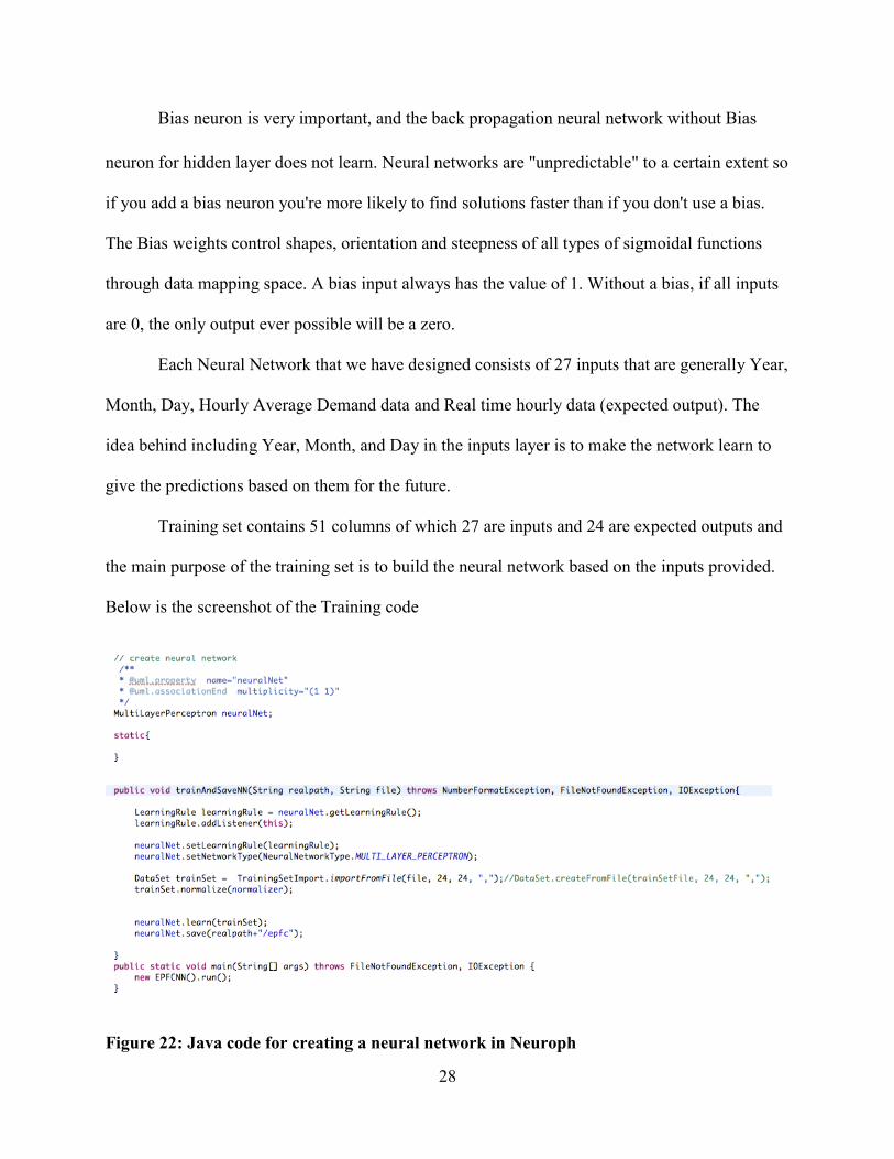
Bias neuron is very important, and the back propagation neural network without Bias
neuron for hidden layer does not learn. Neural networks are "unpredictable" to a certain extent so
if you add a bias neuron you're more likely to find solutions faster than if you don't use a bias.
The Bias weights control shapes, orientation and steepness of all types of sigmoidal functions
through data mapping space. A bias input always has the value of 1. Without a bias, if all inputs
are 0, the only output ever possible will be a zero.
Each Neural Network that we have designed consists of 27 inputs that are generally Year,
Month, Day, Hourly Average Demand data and Real time hourly data (expected output). The
idea behind including Year, Month, and Day in the inputs layer is to make the network learn to
give the predictions based on them for the future.
Training set contains 51 columns of which 27 are inputs and 24 are expected outputs and
the main purpose of the training set is to build the neural network based on the inputs provided.
Below is the screenshot of the Training code
Figure 22: Java code for creating a neural network in Neuroph
Page 40
29
The test/validation set also contains the same number of inputs as training set while the
purpose of the test set is to validate the network that is built during the training phase that returns
the total mean square error between the actual output and the expected output. Below is the
screenshot of the test code
Figure 23: Java code for testing a neural network in Neuroph
In Neuroph, The Neural network is trained with hourly data for years 2009 till 2014 and
tested with 2015 set. Both Training Sets and Test sets are represented by. tset file extension.
Below is the example of training set
5.4. Preprocessing input data
Data used to train and test the neural network should be normalized before feeding to the
network. After collecting the data from ISO-NE express website, we generally do the following
steps
1. Flattening data
Page 41
30
2. Average calculator
3. Normalization
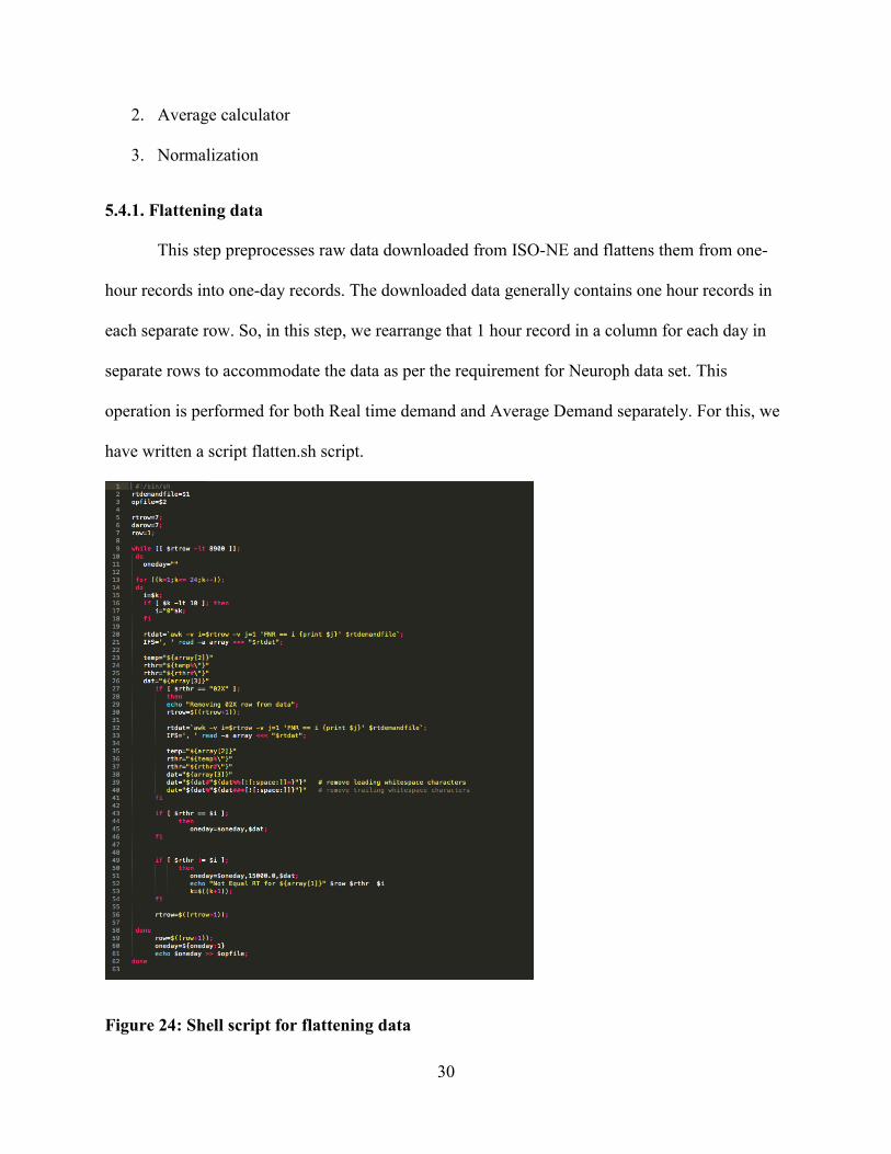
5.4.1. Flattening data
This step preprocesses raw data downloaded from ISO-NE and flattens them from one-
hour records into one-day records. The downloaded data generally contains one hour records in
each separate row. So, in this step, we rearrange that 1 hour record in a column for each day in
separate rows to accommodate the data as per the requirement for Neuroph data set. This
operation is performed for both Real time demand and Average Demand separately. For this, we
have written a script flatten.sh script.
Figure 24: Shell script for flattening data
Page 42
31
5.4.2. Average calculator
In this step, we take the output from previous step of flattening data and calculate the
average demand for 24 hours in separate columns by summing up the demand for the previous 7
days per each single hour separately for that year alone plus previous year’s occurrence of the
very same day. For example, to calculate the input of 1st hour of January 1st 2015, we take an
average demand for the Dec 31st first hour, Dec 30th first hour, Dec 29th first hour, Dec 28th first
hour, Dec 27th first hour , Dec 26th first hour, Dec 25th first hour plus January 1st 2014 first hour,
January 1st 2013 first hour, January 1st 2012 first hour, January 1st 2011 first hour, January 1st
2010 first hour, January 1st 2009 first hour, January 1st 2008 first hour.
Figure 25: Shell script for average calculator
Page 43
32
5.4.3. Normalization
Normalization is a process of converting real data into data that neural networks can
understand and work. Simply put, it is a mapping of real data to data between 0 and 1.
By running epfc-normalizer.jar, we can obtain all the demand values in between 0 and 1
that we can further pass it to the training and test stages. The algorithm that we used to normalize
the data is MiniMax. Below is the Formula:
Figure 26: Normalization step with min max formula
After successfully passing through the training and test phases, we actually can enter the
input data that just contains the average demand to execute and provide us with the output of the
expected demand for the next one-hour or day based on the inputs provided.
Page 44
33
CHAPTER 6. ELECTRICITY DEMAND PREDICTION WITH NEUROPH
6.1. Software simulation
1) Download the Neuroph Studio from the location NeurophStudio
Figure 27: Setting up Neuroph for the Electricity Demand forecasting project
2) Unzip the file
Figure 28: Unzipping the Neuroph Studio
3) Go to neurophstudio->bin and launch the application neurophstudio.exe or
neurophstudio64.exe. For MAC execute neourophstudio.sh script to launch application. You
should be able to see the EDP-055715 project loaded in your workspace as below.
Page 45
34
Figure 29: Successfully installed Neuroph studio
If the project is not loaded default, click on File-> Open Project and select the project
location as neourophstudio -> EDP-055715 as below
Figure 30: Navigate to EDP project
Page 46
35
You can see the EDP-055715 neural network, Training Sets and the Test Set in your
workspace now. On clicking the EDP-055715, opens the neural network design view for you.
Now click on any Training set file to train network and click on train button as below. You can
set the Max error, Learning rate and momentum to train in the dialog box and click on the train
button.
Figure 31: Setting up the learning parameters for electricity demand forecasting
You can see the network getting trained and also the number of iterations it took to get
trained with total network error.
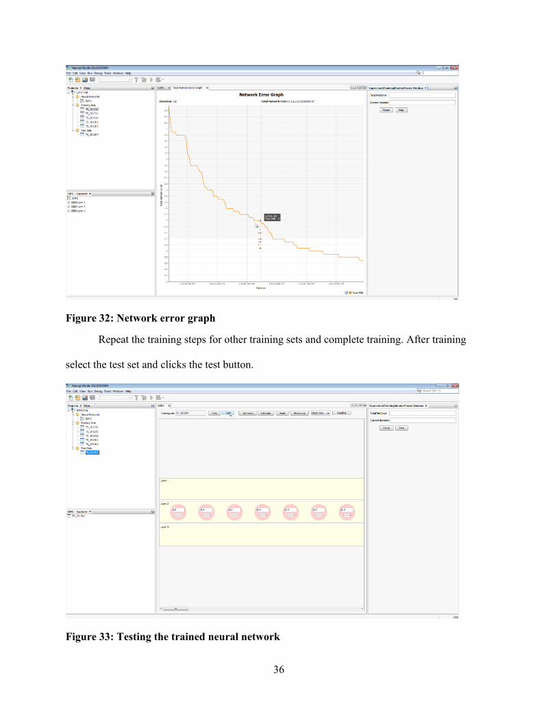
Page 47
36
Figure 32: Network error graph
Repeat the training steps for other training sets and complete training. After training
select the test set and clicks the test button.
Figure 33: Testing the trained neural network
Page 48
37
You can view the results right away with input given, actual output, desired output and
Total Mean square error.
Figure 34: Output after training and testing
This process of training and testing will be repeated for several attempts with varying
learning parameters such as learning rate, momentum and number of hidden neurons to find out
the best network architecture to use it for the final forecast. Per each individual training set, we
can find the best architecture and then we can cross validate the network accuracy.
6.2. Analysis on the training attempts
In this step, our goal is to get the best neural network architecture that has the least total
square error, which would also provide us with the optimum number of hidden neurons that
should be used for the network. Also, while performing this step, we would modify parameters
such as momentum and learning rate to train the network. Data for the years 2009 till 2014 is fed
to the neural network during the train phase and the error that we generate during the training
Page 49
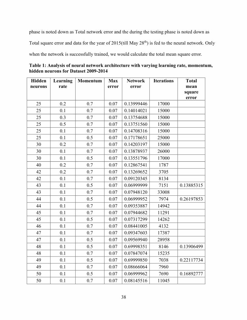
38
phase is noted down as Total network error and the during the testing phase is noted down as
Total square error and data for the year of 2015(till May 28th) is fed to the neural network. Only
when the network is successfully trained, we would calculate the total mean square error.
Table 1: Analysis of neural network architecture with varying learning rate, momentum,
hidden neurons for Dataset 2009-2014
Hidden
neurons
Learning
rate
Momentum Max
error
Network
error
Iterations Total
mean
square
error
25 0.2 0.7 0.07 0.13999446 17000
25 0.1 0.7 0.07 0.14014021 15000
25 0.3 0.7 0.07 0.13754688 15000
25 0.5 0.7 0.07 0.13751560 15000
25 0.1 0.7 0.07 0.14708316 15000
25 0.1 0.5 0.07 0.17178651 25000
30 0.2 0.7 0.07 0.14203197 15000
30 0.1 0.7 0.07 0.13878937 26000
30 0.1 0.5 0.07 0.13551796 17000
40 0.2 0.7 0.07 0.12867541 1787
42 0.2 0.7 0.07 0.13269652 3705
42 0.1 0.7 0.07 0.09120345 8134
43 0.1 0.5 0.07 0.06999999 7151 0.13885315
43 0.1 0.7 0.07 0.07948120 33008
44 0.1 0.5 0.07 0.06999952 7974 0.26197853
44 0.1 0.7 0.07 0.09353887 14942
45 0.1 0.7 0.07 0.07944682 11291
45 0.1 0.5 0.07 0.07317299 14262
46 0.1 0.7 0.07 0.08441005 4132
47 0.1 0.7 0.07 0.09347603 17387
47 0.1 0.5 0.07 0.09569940 28958
48 0.1 0.5 0.07 0.69998351 8146 0.13906499
48 0.1 0.7 0.07 0.07847074 15235
49 0.1 0.5 0.07 0.69999850 7038 0.22117734
49 0.1 0.7 0.07 0.08666064 7960
50 0.1 0.5 0.07 0.06999962 7690 0.16892777
50 0.1 0.7 0.07 0.08145516 11045
Page 50
39
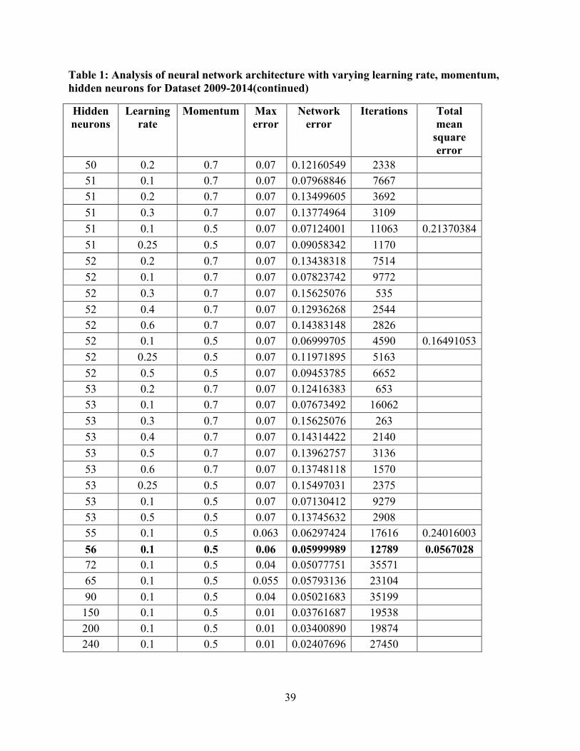
Table 1: Analysis of neural network architecture with varying learning rate, momentum,
hidden neurons for Dataset 2009-2014(continued)
Hidden
neurons
Learning
rate
Momentum Max
error
Network
error
Iterations Total
mean
square
error
50 0.2 0.7 0.07 0.12160549 2338
51 0.1 0.7 0.07 0.07968846 7667
51 0.2 0.7 0.07 0.13499605 3692
51 0.3 0.7 0.07 0.13774964 3109
51 0.1 0.5 0.07 0.07124001 11063 0.21370384
51 0.25 0.5 0.07 0.09058342 1170
52 0.2 0.7 0.07 0.13438318 7514
52 0.1 0.7 0.07 0.07823742 9772
52 0.3 0.7 0.07 0.15625076 535
52 0.4 0.7 0.07 0.12936268 2544
52 0.6 0.7 0.07 0.14383148 2826
52 0.1 0.5 0.07 0.06999705 4590 0.16491053
52 0.25 0.5 0.07 0.11971895 5163
52 0.5 0.5 0.07 0.09453785 6652
53 0.2 0.7 0.07 0.12416383 653
53 0.1 0.7 0.07 0.07673492 16062
53 0.3 0.7 0.07 0.15625076 263
53 0.4 0.7 0.07 0.14314422 2140
53 0.5 0.7 0.07 0.13962757 3136
53 0.6 0.7 0.07 0.13748118 1570
53 0.25 0.5 0.07 0.15497031 2375
53 0.1 0.5 0.07 0.07130412 9279
53 0.5 0.5 0.07 0.13745632 2908
55 0.1 0.5 0.063 0.06297424 17616 0.24016003
56 0.1 0.5 0.06 0.05999989 12789 0.0567028
72 0.1 0.5 0.04 0.05077751 35571
65 0.1 0.5 0.055 0.05793136 23104
90 0.1 0.5 0.04 0.05021683 35199
150 0.1 0.5 0.01 0.03761687 19538
200 0.1 0.5 0.01 0.03400890 19874
240 0.1 0.5 0.01 0.02407696 27450
Page 51
40
From the above table, choose a row that has the least total mean square error and it is the
best network architecture with the data that we trained and tested and is cross validated in our
next step. So, we chose 56 hidden neurons with 0.1 of learning rate and 0.5 of momentum as the
best network architecture. Below are the screenshots, the first one displays the number of
iterations vs error rate graph and the second one displays the total mean square error for that
network.
Figure 35: Test results from the best neural network architecture with 56 neurons
Page 52
41
Figure 36: Total network error graph after successfully training and testing the neural
network
Below is the neural network architecture with 56 hidden neurons.
Figure 37: Neural network architecture with 56 hidden neurons
6.3. Cross-validation
The cross-validation method that we choose for this Neuroph project is leave one out
method where we pick twelve random inputs one from each month for a period of a year (2009)
Page 53
42
and then build test sets leaving one input for each time and repeating it for 12 times until we
cover all the inputs and then calculate the standard deviation and variance for that network.
Cross-validation is an important step that will help us in reporting the variance and standard
deviation of the data. Below is the cross validated data for the 12 experiments performed
Once the network is cross validated, we will take that network to predict the demand for
the past/future and then verify it with the real time demand and forecasted demand in ISO-NE
website. Below is the table showing the hourly-predicted demand for May 29th using Neuroph.
Table 2: Cross-validation with twelve sets of test data
Data sets Total mean square error
Test Data Set – 1 0.0031850865139329016
Test Data Set – 2 0.0036249392444056183
Test Data Set – 3 0.003828890021327136
Test Data Set – 4 0.003710398093381868
Test Data Set – 5 0.0035713844627581477
Test Data Set – 6 0.0038351210994040045
Test Data Set – 7 0.0030103306281517458
Test Data Set – 8 0.0038090656323832503
Test Data Set – 9 0.0035746664332910465
Test Data Set – 10 0.0037918154808452564
Test Data Set – 11 0.0038575024346391147
Test Data Set – 12 0.0034210038689849102
Average 0.0036016836594587
Standard deviation 0.00026150538639467
Variance 6.8385067113428E-8
Page 54
43
Table 3: Forecast with Neuroph vs real time demand.
Hour ending Forecast with Neuroph Real time demand
1 11385.74 12766.6
2 11134.21 12466.33
3 10968.93 12348.47
4 11063.69 12203.43
5 11085.12 12331.7
6 11365.32 12817.61
7 11958.44 13147.62
8 12842.7 14405.13
9 13702.04 15198.16
10 14439.24 15761.09
11 14995.66 16240.08
12 15381.65 16591.85
13 15656.06 16775.99
14 15897.8 17060.35
15 16057.7 17249.15
16 16286.2 17490.01
17 16719.76 17671.23
18 16937.34 17492.3
19 16432.65 16893.26
20 15999.28 16270.22
21 15841.13 16156.64
22 15047.4 15538.65
23 13705.82 14242.28
24 12462.75 13051.38
SUM 325980.89 349402.93
Page 55
44
In order to make sure that the predictions are not always over shooting or undershooting,
we have predicted for some random days and then measured the accuracy of the forecast by
calculating the mean forecast error for 24 hours as shown in the table below.
Table 4: Comparision of forecast with artificial neural network output vs real time demand
6.4. Analysis with Linear Regression
This experiment is designed to determine how well our neural network model works
when compared to linear regression, below are the results for the 1st hour computed with linear
regression to build a function in the forms of y=aX+b using the data from 2009-2014, where X is
Day Forecast (sum of
24hrs in mw)
Real time (sum of
24hrs in mw)
Error
Oct 9th, 2014 325663.18 318128.58 -7534.6
Nov 4th, 2014 322671.83 327464.16 4792.33
Dec 17th, 2014 366270.26 361017.15 -5253.11
Jan 5th, 2015 374508.02 371265.3 -3242.72
Jan 28th, 2015 394050.84 382366.22 -11684.62
Feb 5th, 2015 377972.69 398607.65 20634.96
March 15th, 2015 322708.83 329221.66 6512.83
March 30th, 2015 340483.64 356672.79 16189.15
April 2nd, 2015 341456.41 335478.922 -134.7515
April 21st, 2015 309575.21 313005.73 3430.52
May 6th, 2015 296832.1 307860.47 11028.37
May 30th, 2015 351544.35 345259.35 -6285
June 5th, 2015 328742.14 313587.88 -15154.26
Summation of error 13568.6015
Mean forecast error for 24 hours is 1023.00758
Page 56
45
averages calculated for the past seven days along with the occurrence of the same day in
previous calendar year and y is the real time data. The values of the slope, intercept, correlation
and r2 values are 0.625677, 4618.58931, 0.78193757, 0.61142636 and the equation obtained
from the final output y=0.9772x+282.02, where a=0.9772,b=282.02
Figure 38: Linear Regression for average demand with real time demand
X is the average value evaluated for the first hour, rt is real time demand, lr is linear
regression, ann-artificial neural network, rt-ann indicates difference of output from real time
demand with artificial neural network output, rt-lr indicates difference of output from real time
demand with linear regression output.
y = 0.9772x + 282.02R² = 0.6114
0
5000
10000
15000
20000
25000
0 5000 10000 15000 20000
Linear (Series1)
Page 57
46
Table 5: Analysis of forecast with artificial neural network output vs real time demand vs
Linear Regression.
So, from the above table it is clear that neural network results are much closer to the
output that we get from linear progression.
DAY,
2015
x RT LR ANN RT-ANN RT-LR
Jan 5th 13346.7143 12122.86 13255.0263 13491.91 -1369.05 -1132.1663
Jan 28th
13509.2286 14125.04 13412.9902 14113.5 11.54 712.049800
8
Feb 5th
13897.6914 13878.08 13790.5760
4
13647.1 230.98 87.5039592
March 15th
12375.13 12030.33 12310.6463
6
11673.95 356.38 -280.31636
March 30th
12122.545 12461.51 12065.1337
4
12228.21 233.3 396.37626
April 2nd
12199.2057 12448.26 12139.6479
4
12199.20
57
249.0543 308.612059
6
April 21st
10647.5957 11442 10631.4830
2
10997.76 444.24 810.516979
6
May 6th
10447.1121 10571.64 10436.6129
6
10543.27 28.37 135.027038
8
May 30th
11655.7507 11963.4 11611.4096
8
11962.16 1.24 351.990319
6
June 5th
11410.1807 10827.86 11372.7156
4
11308.14 -480.28 -544.855640
-294.2257 844.738117
6
Page 58
47
CHAPTER 7. ELECTRICITY DEMAND PREDICTION ON WEB
Using the development version of Neuroph framework, a web application is built very
specific to our problem and hosted on Amazon web services. Here is the link for the Source files
of the development version uploaded in GIT repository: https://github.com/sowpar18/edp
Here is the link to the application: http://edp-1034583199.us-west-
2.elb.amazonaws.com/edp/. Below are the steps we can follow to build neural network
architecture on web.
7.1. Create MLP neural network
Enter the number of hidden neurons that you would like to train/test the neural network
as shown in the screenshot below. As you can notice, we have definite input and output neurons
as 27 and 24 respectively.
Figure 39: Creating a multilayer perceptron neural network
Below is the screenshot of the java class that’s corresponding to creating a neural
network.
Page 59
48
Figure 40: Java code for creating a neural network
7.2. Upload datasets
Enter the name of the training set and upload the data set by clicking on upload
Figure 41: Uploading training set
Below is the screenshot of the java class responsible for the upload datasets.
Page 60
49
Figure 42: Java code for uploading training set
7.3. Train neural network
Train the neural network by selecting the network that was created in 7.2.1 step i.e.
Create Neural Network and select the data set that was uploaded in 7.2.2 step i.e. upload data set.
Enter the max number of iterations and then enter max error, learning rate and momentum.
Figure 43: Training a neural network
Below is the screenshot of the source code for Training Neural network.
Page 61
50
Figure 44: Java code for training a neural network
Click on logs to see the training iterations that are going through the network as shown in
the below screenshot
Page 62
51
Figure 45: Training logs generated from a neural network during the training phase
7.4. Test neural network
Once training is done successfully, we need to test the neural network to find out the best
neural network as shown in the below screenshot.
Page 63
52
Figure 46: Testing a neural network
Click on test button to test the neural network and you can see the total mean square error
for that network. Below is the screenshot of the test source code.
Page 64
53
Figure 47: Java code for testing a neural network
7.5. Cross-validate neural network
Once the successfully trained networks are tested, we will get a list of networks with total
mean square errors and we pick the network that has the least total mean square error to cross
validate the accuracy of the network by leave one out method. Below is the screenshot.
Page 65
54
Figure 48: Cross-validating a neural network
Below is the source code for cross-validate class
Figure 49: Java code for cross-validation
Page 66
55
7.6. Predict demand
We can predict the demand for future by uploading a new dataset and feed it to the same
network and click on predict as shown in the below screenshot.
Figure 50: Predicting electricity demand
On clicking predict, we would see an output from the network for the 24 hours arranged
in each single row as shown in the below screenshot.
Page 67
56
Figure 51: Output of electricity demand after it’s predicted
Below is the screenshot of the source code for predicting class of the neural network.
Page 68
57
Figure 52: Java code for electricity demand prediction
Page 69
58
CHAPTER 8. CONCLUSION AND FUTURE WORK
This paper discusses the concept of building best neural network model with a neural
network framework using historical data that can help distributors or utility companies in
preparing better for the future electricity demand requirements.
The overall goal of the project was to build a tool that predicts the electricity demand for
day ahead given large amount of historical data. Historical data ranging from 2007-2015(till
date) is used to train and test the neural network for future predictions.
From the experimental results, high performance neural network model has been
successfully built which produced close predictions to the real time demand with a reasonable
number of iterations and acceptable error rates of 0.06. Accuracy of the prediction was cross-
validated with reasonable standard deviation and variance. Mean forecast errors were calculated
to verify the overall forecast accuracy with a difference of 1023 mw of electricity demand for 24
hours. Also, the neural network model’s accuracy is much better than linear regression method
on a limited number experiments.
Training data that is available on the ISO-NE express website is for only 8 years and
hence future work would be to collect more data for some additional years and run the neural
network training phase and possibly build a network that has an error rate of less than 0.01.
An interesting problem to solve is to expand the problem space to predict the demand
based on individual regions across New England along with the consideration of economic
factors and weather conditions would also be a challenging task to accomplish as enhancements.
Page 70
59
REFERENCES
Čutović, I. (n.d.). Glass identification using neural networks. Retrieved from
neuroph.sourceforge.net:
http://neuroph.sourceforge.net/tutorials/GlassIdentification/GlassIdentificationUsingNeuralNetw
orks.html
A.C.Andersen. (2010). Autonomous neural development and pruning. Retrieved from
http://blog.andersen.im/wp-
content/uploads/2010/12/AutonomousNeuralDevelopmentAndPruning-AndersenAC.pdf
AbuAl-Foul, B. M. (2012). Forecasting energy demand in Jordan using artificial neural
networks.
Alexandre, M., & Edson, C. (2010). FIVE-framework for an integrated voice environment.
IWSSIP-2010.
Angelini, E., di Tollo, G., & Roli, A. (2008). A nueral network approach for credit risk
evaluation.
AZOFF, M. E. (1994). Neual network time series forecasting of financial markets.
Bacha, H., & Meyer, W. (1992). A Neural network architecture for load forecasting. Proceedings
of international joint conference on neural networks.
Castro, L. I., & Cramton, P. (2009). Prediction markets to forecast electricity. 19.
Chow, M., & TRAM, H. Application of fuzzy logic technology for spatial load forecasting.
EIA. (n.d.). Annual energy outlook. Retrieved from http://www.eia.gov/:
http://www.eia.gov/forecasts/aeo/MT_electric.cfm
Ferlito, S. e. (2015). Predictive models for building's energy consumption: an artificial neural
network (ANN) approach. AISEM Annual conference, 2015 XVIII (pp. 1-4). Trento: IEEE.
Francisco J. Nogales, J. C. (2002). Forecasting next-day electricity prices by time series models.
IEEE Transactions on power systems , 6.
Gately, E. (1996). Neural networks for financial forecasting.
Granger, C. W., & Terasvirta, T. (1993). Modelling nonlinear economic relationships.
Haixun, W., Shijun, L., Satoshi , O., Xiaohua, H., & Tieyun, Q. (2011). Efficient name
disambiguation in digital libraries. Proceedings of the 12th international conference on web-age
information management. Berlin: Springer-Verlag.
Page 71
60
Heaton, J. (2010, feb 9). Basic market forecasting with encog neural networks. Retrieved from
www.devx.com: http://www.devx.com/opensource/Article/44014
Heaton, J. (2008). Introduction to neural networks for java, Second Edition. Jeff Heaton.
Hernandez, G., & Salinas, L. (2004). Large scale simulations of a neural network model for the
graph bisection problem on geometrically connected graphs.
hoseinzade, S., & Akhavan Niaki, S. (2013). Forecasting S&P 500 index using artificial neural
networks and design of experiments.
Hyde, O., & Hodnett, P. F. (1997). An adaptable automated procedure for short-term electricity
load forecasting.
Hyndman, R. J. (2011, October 3). Forecasting electricity demand distributions using a
semiparametric additive model. Retrieved from http://robjhyndman.com/talks/electricity-
forecasting/.
Ivanić, N. (n.d.). Predicting poker hands with neural networks. Retrieved from
neuroph.sourceforge.net:
http://neuroph.sourceforge.net/tutorials/PredictingPokerhands/Predicting%20poker%20hands%2
0with%20neural%20networks.htm
J.P.S. Catalao, S. .. (2006). Short-term electricity prices forecasting in a competitive market.
ELSEVIER , 7.
JayaKumar, K. R., & Alain, A. (2013). A survey of software test estimation techniques.
Scientific Research .
Jeremic, M. (n.d.). Music classification by genre using neural networks. Retrieved from
neuroph.sourceforge.net:
http://neuroph.sourceforge.net/tutorials/MusicClassification/music_classification_by_genre_usin
g_neural_networks.html
Jovanovic, A. (n.d.). Blood transfusion service center. Retrieved from neuroph.sourceforge.net:
http://neuroph.sourceforge.net/tutorials/BloodTransfusionSc/blood_transfusion_sc.html
Jovanovic, M. (n.d.). Predicting the class of haberman's survival with neural networks .
Retrieved from neuroph.sourceforge.net:
http://neuroph.sourceforge.net/tutorials/HebermanSurvival/HabermansSurvival.html
Küçükdeniz, T. (2010). Long term electricity demand forecasting: an alternative approach with
support vector machines. Academia.edu .
Page 72
61
Kandananond, K. (2011). Forecasting electricity demand in Thailand with an artificial neural
network approach. MDPI Energies .
Kargar, M. J., & charsoghi, D. (2014). Predicting annual electricity consumption in iran using
artificial neural networks (NARX).
Kumar, P. C., & Walia, E. (2006). Cash forecasting: an application of artificial neural networks
in finance.
Levine, D. (2006). Neural modeling of the dual motive theory of economics. Journal of Socio
economics.
Limanond, T., Jomnokwao, S., & Srikaew, A. (2011). Projection of future transport energy
demand of Thailand. Energy Policy .
Lisboa, P. J., & Taktak, A. F. (2006). The use of artificial neural networks in decision support in
cancer: a systematic review.
Mitrea, C. A., Lee, C. K., & Wu, Z. (2009). A comparision between neural networks and
traditional forecasting methods: a case study. International journal of engineer business
management, vol.1, no.2 .
National Grid. Understanding electricity demand.
Palmer, A., Montano, J. J., & Sese, A. (2006). Designing an artificial neural network approach
for forecasting tourism time series. Tourism management.
Pankilb, K., Prakasvudhisarn, C., & Khummongkol, D. (2015). Electricity consumption
forecasting in Thailand using an artificial neural network and multiple linear regression. 10 (4),
427-434.
Patuwo, E. B., Zhang, G., & Hu, M. Y. (1997). Forecasting with artificial neural networks: the
state of the art. Internation Journal of forecasting 14 .
Pierre, S., Said, H., & Probst, W. G. (2001). An artificial neural network approach for routing in
distributed computer networks. Engineering Applications of Artificial Intelligence.
Prasad, B. (2008). Soft computing applications in industry. Springer.
Quek, M., & Moskowitz, D. (2007). Testing neural network models of personality. Journal of
research in personality.
Radovanović, S., & Radojičić, ,. M. (n.d.). Predicting the result of football match with neural
networks. Retrieved from neuroph.sourceforge.net:
http://neuroph.sourceforge.net/tutorials/SportsPrediction/Premier%20League%20Prediction.html
Page 73
62
Refenes, A.-P. (1995). Neural networks in the capital markets.
Risteski, S. (n.d.). Recognition of Braille using neural networks. Retrieved from
neuroph.sourceforge.net:
http://neuroph.sourceforge.net/tutorials/Braille/RecognitionOfBrailleAlphabetUsingNeuralNetw
orks.html
Rodrigues, F., Cardeira, C., & Calado, J. M. (2014). The daily and hourly energy consumption
and load forecasting using artificial neural network method: a case study using a set of 93
households in Portugal.
Severac, Z. (2011). Neural networks on the netbeans platform. Retrieved from Oracle:
http://www.oracle.com/technetwork/articles/java/nbneural-317387.html
Smith, K. A., & Gupta, J. N. (2002). Neural networks in business: techniques and applications.
Idea group publishing.
Stojilkovic, J. (n.d.). Face recognition using neural network. Retrieved from
neuroph.sourceforge.net:
http://neuroph.sourceforge.net/tutorials/FaceRecognition/FaceRecognitionUsingNeuralNetwork.
html
Stojković, M. (n.d.). Wine classification using neural networks. Retrieved from
neuroph.sourceforge.net:
http://neuroph.sourceforge.net/tutorials/wines1/WineClassificationUsingNeuralNetworks.html
Taheri, T. (2010, June 3). Benchmarking and comparing Encog, Neuroph and JOONE neural
networks. Retrieved from www.codeproject.com:
http://www.codeproject.com/Articles/85487/Benchmarking-and-Comparing-Encog-Neuroph-
and-JOONE
Trippi, R. R., & Turban, E. (1992). Neural networks in finance and investing.
Trisic, J. (n.d.). Predicting the class of breast cancer with neural networks. Retrieved from
neuroph.sourceforge.net:
http://neuroph.sourceforge.net/tutorials/PredictingBreastCancer/PredictingBreastCancer.html
U.S. Department of Energy. (2007). The smart grid: an introduction. U.S. Department of
Energy.
U.S. Department of Energy, SmartGrid. (2008). What the smart grid means to Americans.
Urosevic, M. (n.d.). Lenses classification using neural networks. Retrieved from
neuroph.sourceforge.net:
Page 74
63
http://neuroph.sourceforge.net/tutorials/LensesClassification/LensesClassificationUsingNeuralN
etworks.html
Zhu, J. (2015). Optimization of power system operation. Wiley-IEEE Press; 2 edition.