Electricity price modeling and asset valuation: a multi-fuel structural approach Article (Accepted Version) http://sro.sussex.ac.uk Carmona, René, Coulon, Michael and Schwarz, Daniel (2013) Electricity price modeling and asset valuation: a multi-fuel structural approach. Mathematics and Financial Economics, 7 (2). pp. 167-202. ISSN 1862-9679 This version is available from Sussex Research Online: http://sro.sussex.ac.uk/45721/ This document is made available in accordance with publisher policies and may differ from the published version or from the version of record. If you wish to cite this item you are advised to consult the publisher’s version. Please see the URL above for details on accessing the published version. Copyright and reuse: Sussex Research Online is a digital repository of the research output of the University. Copyright and all moral rights to the version of the paper presented here belong to the individual author(s) and/or other copyright owners. To the extent reasonable and practicable, the material made available in SRO has been checked for eligibility before being made available. Copies of full text items generally can be reproduced, displayed or performed and given to third parties in any format or medium for personal research or study, educational, or not-for-profit purposes without prior permission or charge, provided that the authors, title and full bibliographic details are credited, a hyperlink and/or URL is given for the original metadata page and the content is not changed in any way.
Transcript
Electricity price modeling and asset valuation: a multi-fuel structural approach
Article (Accepted Version)
http://sro.sussex.ac.uk
Carmona, René, Coulon, Michael and Schwarz, Daniel (2013) Electricity price modeling and asset valuation: a multi-fuel structural approach. Mathematics and Financial Economics, 7 (2). pp. 167-202. ISSN 1862-9679
This version is available from Sussex Research Online: http://sro.sussex.ac.uk/45721/
This document is made available in accordance with publisher policies and may differ from the published version or from the version of record. If you wish to cite this item you are advised to consult the publisher’s version. Please see the URL above for details on accessing the published version.
Copyright and reuse: Sussex Research Online is a digital repository of the research output of the University.
Copyright and all moral rights to the version of the paper presented here belong to the individual author(s) and/or other copyright owners. To the extent reasonable and practicable, the material made available in SRO has been checked for eligibility before being made available.
Copies of full text items generally can be reproduced, displayed or performed and given to third parties in any format or medium for personal research or study, educational, or not-for-profit purposes without prior permission or charge, provided that the authors, title and full bibliographic details are credited, a hyperlink and/or URL is given for the original metadata page and the content is not changed in any way.
2 ELECTRICITY PRICE MODELING AND ASSET VALUATION: A MULTI-FUEL STRUCTURAL APPROACH
captures the dependency of power prices on their primary drivers; yet we obtain closed-form
expressions for spot, forward and option prices.
The existing literature on electricity price modeling can be approximately divided into three
categories. At one end of the spectrum are so called full production cost models. These rely
on knowledge of all generation units, their corresponding operational constraints and network
transmission constraints. Prices are then typically solved for by complex optimization routines
(cf. [21]). Although this type of model may provide market insights and forecasts in the short
term, it is — due to its complexity — unsuited to handling uncertainty, and hence to derivative
pricing or the valuation of physical assets. Other related approaches which share this weakness
include models of strategic bidding (cf. [24]) and other equilibrium approaches (cf. [6]). At the
other end of the spectrum are reduced form models. These are characterised by an exogenous
specification of electricity prices, with either the forward curve (cf. [14] and [5]) or the spot price
(cf. [18, 11, 22, 4]) representing the starting point for the model. Reduced form models typically
either ignore fuel prices or introduce them as exogenous correlated processes; hence they are not
successful at capturing the important afore mentioned dependence structure between fuels and
electricity. Further, spikes are usually only obtained through the inclusion of jump processes
or regime switches, which provide little insight into the causes that underly these sudden price
swings.
In between these two extremes is the structural approach to electricity price modeling, which
stems from the seminal work of Barlow [3]. We use the adjective structural to describe models,
which — to varying degrees of detail and complexity — explicitly approximate the supply curve
in electricity markets (commonly known as the bid stack due to the price-setting auction). The
market price is then obtained under the equilibrium assumption that demand and supply must
match. In Barlow’s work the bid stack is simply a fixed parametric function, which is evaluated
at a random demand level. Later works have refined the modeling of the bid curve and taken
into account its dependency on the available capacity (cf. [8, 7, 12]), as well as fuel prices
(cf. [29, 16, 1, 2]) and the cost of carbon emissions (cf. [25, 15]). The raison d’etre of all
structural models is very clear. If the bid curve is chosen appropriately, then observed stylized
facts of historic data can be well matched. Moreover, because price formation is explained
using fundamental variables and costs of production, these models offer insight into the causal
relationships in the market; for example, prices in peak hours are most closely correlated with
natural gas prices in markets with many gas ‘peaker’ plants; similarly, price spikes are typically
observed to coincide with states of very high demand or low capacity. As a direct consequence,
this class of models also performs best at capturing the varied dependencies between electricity,
fuel prices, demand and capacity.
The model we propose falls into the category of structural models (see [9] for a recent survey of
this category). Our work breaks from the current status quo by providing closed-form formulae
for the prices of a number of derivative products in a market driven by two underlying fuels
and featuring a continuum of efficiencies (heat rates). In the considered multi-fuel setting, our
model of the bid stack allows the merit order to be dynamic: each fuel can become the marginal
fuel and hence set the market price of electricity. Alternatively, several fuels can set the price
jointly. Despite this complexity, under only mild assumptions on the distribution, under the
pricing measure, of the terminal value of the processes representing electricity demand and fuels,
we obtain explicit formulae for spot prices, forwards and spread options, as needed for power
ELECTRICITY PRICE MODELING AND ASSET VALUATION: A MULTI-FUEL STRUCTURAL APPROACH 3
plant valuation. Moreover, our formulae capture very clearly and conveniently the dependency
of electricity derivatives upon the prices of forward contracts written on the fuels that are used
in the production process. This allows the model to easily ‘see’ additional information contained
in the fuel forward curves, such as states of contango or backwardation — another feature, which
distinguishes it from other approaches.
The parametrization of the bid stack we propose combines an exponential dependency on de-
mand, suggested several times in the literature (cf. [32, 13, 26]), with the need for a heat rate
function multiplicative in the fuel price, as stressed by Pirrong and Jermakyan [29]. Eydeland
and Geman [20] propose a similar structure for forward prices and note that Black-Scholes
like derivative prices are available if the power price is log-normal. However, this requires the
assumption of a single marginal fuel type and ignores capacity limits. Coulon and Howison
[16] construct the stack by approximating the distribution of the clusters of bids from each
technology, but their approach relies heavily on numerical methods when it comes to derivative
pricing. In the work of Aid et al [1], the authors simplify the stack construction by allowing
only one heat rate (constant heat rate function) per fuel type, a significant oversimplification
of spot price dynamics for mathematical convenience. Aid et al [2] extend this approach to
improve spot price dynamics and capture spikes, but at the expense of a static merit order,
ruling out, among other things, the possibility that coal and gas can change positions in the
stack in the future. In both cases the results obtained by the authors only lead to semi-closed
form formulae, which still have to be evaluated numerically.
The importance of the features incorporated in our model is supported by prominent devel-
opments observed in recent data. In particular, shale gas discoveries have led to a dramatic
drop in US natural gas prices in recent years, from a high of over $13 in 2008 to under $3 in
January 2012. Such a large price swing has rapidly pushed natural gas generators down the
merit order, and highlights the need to account for uncertainty in future merit order changes,
particularly for longer term problems like plant valuation. In addition, studying hourly data
from 2004 to 2010 on marginal fuels in the PJM market (published by Monitoring Analytics),
we observe that the electricity price was fully set by a single technology (only one marginal fuel)
in only 16.1 per cent of the hours. For the year 2010 alone, the number drops to less than 5
per cent. Substantial overlap of bids from different fuels therefore exists, and changes in merit
order occur gradually as prices move. We believe that our model of the bid stack adheres to
many of the true features of the bid stack structure, which leads to a reliable reproduction of
observed correlations and price dynamics, while retaining mathematical tractability.
2. Structural approach to electricity pricing
In the following we work on a complete probability space (Ω,F ,P). For a fixed time horizon
T ∈ R+, we define the (n + 1)-dimensional standard Wiener process (W 0t ,Wt)t∈[0,T ], where
W := (W 1, . . . ,W n). Let F0 := (F0t ) denote the filtration generated by W 0 and FW := (FW
t )
the filtration generated by W. Further, we define the market filtration F := F0 ∨ FW . All
relationships between random variables are to be understood in the almost surely sense.
2.1. Price Setting in Electricity Markets. We consider a market in which individual firms
generate electricity. All firms submit day-ahead bids to a central market administrator, whose
task it is to allocate the production of electricity amongst them. Each firm’s bids take the form
4 ELECTRICITY PRICE MODELING AND ASSET VALUATION: A MULTI-FUEL STRUCTURAL APPROACH
of price-quantity pairs representing an amount of electricity the firm is willing to produce, and
the price at which the firm is willing to sell it1. An important part is therefore played by the
merit order, a rule by which cheaper production units are called upon before more expensive
ones in the electricity generation process. This ultimately guarantees that electricity is supplied
at the lowest possible price.2
Assumption 1. The market administrator arranges bids according to the merit order and
hence in increasing order of costs of production.
We refer to the resulting map from the total supply of electricity and the factors that influence
the bid levels to the price of the marginal unit as the market bid stack and assume that it can
be represented by a measurable function
b : [0, ξ]× Rn ∋ (ξ, s) → b(ξ, s) ∈ R,
which will be assumed to be strictly increasing in its first variable. Here, ξ ∈ R+ represents the
combined capacity of all generators in the market, henceforth the market capacity (measured
in MW), and s ∈ Rn represents factors of production which drive firms’ bids (e.g. fuel prices).
Demand for electricity is assumed to be price-inelastic and given exogenously by an F0t -adapted
process (Dt) (measured in MW). As we shall see later, the prices of the factors of production
used in the electricity generation process will be assumed to be FWt -adapted. So under the
objective historical measure P, the demand is statistically independent of these prices. This is
a reasonable assumption as power demand is typically driven predominantly by temperature,
which fluctuates at a faster time scale and depends more on local or regional conditions than fuel
prices. The market responds to this demand by supplying an amount ξt ∈ [0, ξ] of electricity.
We assume that the market is in equilibrium with respect to the supply of and demand for
electricity; i.e.
(1) Dt = ξt, for t ∈ [0, T ].
This implies that Dt ∈ [0, ξ] for t ∈ [0, T ] and (ξt) is F0t -adapted.
The market price of electricity (Pt) is now defined as the price at which the last unit that is
needed to satisfy demand sells its electricity; i.e. using (1),
(2) Pt := b(Dt, ·), for t ∈ [0, T ].
We emphasize the different roles played by the first variable (i.e. demand) and all subsequent
variables (i.e. factors driving bid levels) of the bid stack function b. Due to the inelastic-
ity assumption, the level of demand fully determines the quantity of electricity that is being
generated; all subsequent variables merely impact the merit order arrangement of the bids.
Remark 1. The price setting mechanism described above applies directly to day-ahead spot
prices set by uniform auctions,3 as in most exchanges today. However, we believe that in a
1Alternatively, firms may, in some markets, submit continuous bid curves, which map an amount of electricityto the price at which it is offered. For our purposes this distinction will however not be relevant.2This description is of course a simplification of the market administrator’s complicated unit commitment prob-lem, typically solved by optimization in order to satisfy various operational constraints of generators, as well astransmission constraints. Details vary from market to market and we do not address these issues here, as our goalis to approximate the price setting mechanism and capture the key relationships needed for derivative pricing.3In a uniform auction all successful bidders pay the same auction clearing price for the amount of electricity theybought.
ELECTRICITY PRICE MODELING AND ASSET VALUATION: A MULTI-FUEL STRUCTURAL APPROACH 5
competitive market with rational agents, the day-ahead auction price also serves as the key
reference point for real-time and over-the-counter prices.
2.2. Mathematical Model of the Bid Stack. From the previous subsection, it is clear that
the price of electricity in a structural model like the one we are proposing depends critically on
the construction of the function b. Before we explain how this is done in the current setting, we
make the following assumption about the formation of firms’ bids.
Assumption 2. Bids are driven by production costs. Furthermore,
(A2.1) costs depend on fuel prices and firm-specific characteristics only;
(A2.2) firms’ marginal costs are strictly increasing.
0 7x 10
4
300
600
Supply (MW)
Pric
e ($
/MW
h)
1st February 20031st March 2003
(a) Sample bid stacks.
0
100
200
2001 2004 2007 2010Year
Pric
e ($
/MW
h)
(b) Historical daily average prices.
Figure 1. Historical prices and bids from the PJM market in the North East US
To back up Assumption 2, we briefly consider it in light of historic bid and spot price data.
Figure 1a plots the bid stack from the PJM market region in the US on the first day of two
consecutive months. Firstly, rapidly increasing marginal costs lead to the steep slope of the stack
near the market capacity (70,000 MW); this feature translates directly into spikes in spot prices
(see Figure 1b) when demand is high. Between the two sample dates in February and March
2003, the prices of gas increased rapidly. In the PJM market gas fired plants have historically
featured mainly in the second half of the bid stack. Therefore, it is precisely the gas price
related increase in production costs, which explains the increase in bid levels observed beyond
about 40,000MW in Figure 1a (see also §4.2 for a discussion of recent merit order changes).
Production costs are typically linked to a particular fuel price (e.g. coal, natural gas, lignite,
oil, etc.). Furthermore, within each fuel class, the cost of production may vary significantly, for
example as old generators may have a higher heat rate (lower efficiency) than new units. It is
not our aim to provide a mathematical model that explains how to aggregate individual bids
or capture strategic bidding. Instead, we group together generators of the same fuel type and
assume the resulting bid curve to be exogenously given and to satisfy Assumption 2. From this
set of bid curves, the merit order rule then determines the construction of the market bid stack.
Let I = 1, . . . , n denote the index set of all the fuels used in the market to generate electricity.
We assume that their prices are the only factors influencing the bid stacks. With each i ∈ I we
6 ELECTRICITY PRICE MODELING AND ASSET VALUATION: A MULTI-FUEL STRUCTURAL APPROACH
associate an FWt -adapted fuel price process (Si
t) and we define the fuel bid curve for fuel i to
be a measurable function
(3) bi : [0, ξi]× R ∋ (ξ, s) → bi(ξ, s) ∈ R,
where the argument ξ represents the amount of electricity supplied by generators utilizing fuel
type i, s a possible value of the price Sit , and ξi ∈ R+ the aggregate capacity of all the generators
utilizing fuel type i. We assume that bi is strictly increasing in its first argument, as required
by Assumption 2. Further, also for i ∈ I, let the F0t -adapted process (ξit) represent the amount
of electricity supplied by generators utilizing fuel type i. It follows that∑
i∈I
ξi = ξ, and Dt =∑
i∈I
ξit, for t ∈ [0, T ].
In order to simplify the notation below, for i ∈ I, and for each s ∈ R we denote by bi( · , s)−1
the generalized (right continuous) inverse of the function ξ → bi(ξ, s). Thus
bi( · , s)−1(p) := ξi ∧ inf
ξ ∈ (0, ξi] : bi(ξ, s) > p
, for (p, s) ∈ R× R,
where we use the standard convention inf ∅ = +∞. Using the notation
bi(s) := bi(0, s) and bi(s) := bi(ξi, s)
and writing b−1i (p, s) = bi( · , s)
−1(p) to ease the notation, we see that b−1i (p, s) = 0 if p ∈
(−∞, bi(s)), b−1i (p, s) = ξi if p ∈ [bi(s),∞), and b−1
i (p, s) ∈ [0, ξi] if p ∈ [bi(s), bi(s)). For fuel
i ∈ I at price Sit = s and for electricity prices below bi(s) no capacity from the ith technology
will be available. Similarly, once all resources from a technology are exhausted, increases in the
electricity price will not lead to further production units being brought online. So defined, the
inverse function b−1i maps a given price of electricity and the price of fuel i to the amount of
electricity supplied by generators relying on this fuel type.
The following simple proposition constructs the market bid stack in the present setting.
Proposition 1. Under assumption 1 and given the definition of the fuel bid curves in (3), with
the definition s = (s1, . . . , sn), the market bid stack is given by
(4) b(ξ, s) := mini∈I
bi(
si)
∨ sup
p ∈ R :∑
i∈I
b−1i
(
p, si)
< ξ
, for (ξ, s) ∈ [0, ξ]× Rn,
where we use the convention sup ∅ = −∞.
Proof. By the definition of b−1i , the function b−1, defined by
b−1(p, s1, · · · , sn) :=∑
i∈I
b−1i (p, si),
is, when the prices of all the fuels are fixed, a non-decreasing map taking the electricity price
to the corresponding amount of electricity generated by the market. Similarly to the case of
one fixed fuel price, for each fixed set of fuel prices, say s := (s1, · · · , sn), we define the bid
stack function ξ → b(ξ, s) as the generalized (left continuous) inverse of the function ξ →
b−1(p, s1, · · · , sn) defined above.
ELECTRICITY PRICE MODELING AND ASSET VALUATION: A MULTI-FUEL STRUCTURAL APPROACH 7
For a given vector (Dt,St), where St := (S1t , . . . , S
nt ) the market price of electricity (Pt) is now
determined by (2) that is,
Pt = b(Dt,St), for t ∈ [0, T ].
2.3. Defining a Pricing Measure in the Structural Setting. The results presented in this
paper do not depend on a particular model for the evolution of the demand for electricity and
the prices of fuels. In particular, the concrete bid stack model for the electricity spot price
introduced in §3 is simply a deterministic function of the exogenously given factors under the
real world measure P. However, for the pricing of derivatives in §4 and §5 we need to define
a pricing measure Q and the distribution of the random factors at maturity under this new
measure will be important for the results that we obtain later.
For an Ft-adapted process θt, where θt := (θ0t , θ1t , . . . , θ
nt ), a measure P ∼ P is characterized by
the Radon-Nikodym derivative
(5)dP
dP:= exp
(
−
∫ T
0θu · dWu −
1
2
∫ T
0|θu|
2 du
)
,
where we assume that (θt) satisfies the so-called Novikov condition
E
[
exp
(
1
2
∫ T
0|θu|
2 du
)]
< ∞.
We identify (θ0t ) and (θit) with the market prices of risk for demand and for fuel i respectively.
We choose to avoid the difficulties of estimating the market price of risk (see for example [21]
for several possibilities) and instead make the following assumption.
Assumption 3. The market chooses a pricing measure Q ∼ P, such that
Q ∈
P ∼ P : all discounted prices of traded assets are P-martingales
.
Note that we make no assumption regarding market completeness here. Because of the non-
storability condition, certainly electricity cannot be considered a traded asset. Further, there
are different approaches to modeling fuel prices; they may be treated as traded assets (hence
local martingales under Q) or — more realistically — assumed to exhibit mean reversion under
the pricing measure. Either way, demand is a fundamental factor and the noise (W 0t ) associated
with it means that the joined market of fuels and electricity is bound to be incomplete. Note
however, that all derivative products that we price later in the paper (forward contracts and
spread options) are clearly traded assets and covered by Assumption 3.
3. Exponential Bid Stack Model
Equation (4) in general cannot be solved explicitly. The reason for this is that any explicit
solution essentially requires the inversion of the sum of inverses of individual fuel bid curves.
We now propose a specific form for the individual fuel bid curves, which allows us to obtain a
closed form solution for the market bid stack b. Here and throughout the rest of the paper, for
i ∈ I, we define bi to be explicitly given by
(6) bi(ξ, s) := s exp(ki +miξ), for (ξ, s) ∈ [0, ξi]× R+,
where ki and mi are constants and mi is strictly positive. Note that bi clearly satisfies (A2.1)
and since it is strictly increasing on its domain of definition it also satisfies (A2.2).
8 ELECTRICITY PRICE MODELING AND ASSET VALUATION: A MULTI-FUEL STRUCTURAL APPROACH
3.1. The Case of n Fuels. For observed (Dt,St), let us define the sets M,C ⊆ I by
M := i ∈ I : generators using fuel i are partially used
and C :=
i ∈ I : the entire capacity ξi of generators using fuel i is used
.
A possible procedure for establishing the members of M and C is to order all the values of biand bi and determine the corresponding cumulative amounts of electricity that are supplied at
these prices. Then find where demand lies in this ordering.
Remark 2. Note that as the merit order and the demand for electricity are both stochastic in
our setting also the sets M and C defined above depend on time and randomness.
With the above definition of M and C we arrive at the following corollary to Proposition 1.
Corollary 1. For bi of exponential form, as defined in (6), the market price of electricity is
given explicitly by the left continuous version of
(7) Pt =
(
∏
i∈M
(
Sit
)αi
)
exp
β + γ
(
Dt −∑
i∈C
ξi
)
, for t ∈ [0, T ],
where
αi :=1
ζ
∏
j∈M,j 6=i
mj
, β :=1
ζ
∑
l∈M
kl∏
j∈M,j 6=l
mj
,
γ :=1
ζ
∏
j∈M
mj
and ζ :=∑
l∈M
∏
j∈M,j 6=l
mj.
Proof. At any time t ∈ [0, T ] the electricity price depends on the composition of the sets M and
C; i.e. the current set of marginal and fully utilized fuel types.
For i ∈ M , b−1i = b−1
i , for i ∈ C, b−1i = ξi and for i ∈ I \M ∪C, b−1
i = 0. Therefore, inside the
supremum in (4), we replace I with M and take∑
i∈C ξi to the right hand side. By Proposition
1 the electricity price is given by the left continuous inverse of the function∑
i∈M b−1i , which in
the exponential case under consideration, simplifies to a single log function and yields (7).
0 q3 q2 q1
Supply (MW)
Pric
e (E
uro/
MW
h)
b1
b2
b3
(a) Fuel bid curves bi.
0 q1+q2 qSupply (MW)
Pric
e (E
uro/
MW
h)
(b) Market bid stack b.
Figure 2. Example of fuel bid curves and resulting market bid stack for I := 1, 2, 3, q := ξ
ELECTRICITY PRICE MODELING AND ASSET VALUATION: A MULTI-FUEL STRUCTURAL APPROACH 9
Pt, for t ∈ [0, T ] CriterionComposition ofM C
Sct exp (kc +mcDt) bc (Dt, S
ct ) ≤ bg (S
gt ) c ∅
Sgt exp (kg +mgDt) bg (Dt, S
gt ) ≤ bc (S
ct ) g ∅
Sct exp
(
kc +mc
(
Dt − ξg))
bc(
Dt − ξg, Sct
)
> bg (Sgt ) c g
Sgt exp
(
kg +mg
(
Dt − ξc))
bg(
Dt − ξc, Sgt
)
> bc (Sct ) g c
(Sct )
αc (Sgt )
αg exp (β + γDt) otherwise c, g ∅
Table 1. Distinct cases for the electricity price (7) in the two fuel case
It is clear from equation (7) that the number of possible expressions for the electricity price is
fully determined by the different configurations the sets M and C can take. In fact, fluctuations
in demand and fuel prices can lead to
(8)n∑
i=1
(
n
i
)
n−i∑
j=0
(
n− i
j
)
distinct cases for (7). Nonetheless, the market bid stack is always a piece-wise exponential
function of demand (see Figure 2) with constantly evolving shape as fuel prices move. This
captures in a very tractable way the influence of fuel prices on the merit order and resulting
power price dynamics.
3.2. The Case of Two Fuels. For the remainder of the paper, we restrict our attention to
the case of a two-fuel market, consisting of coal and natural gas generators. Our results can in
principle be extended to the general case of n > 2 fuels. However, the level of complexity of
the formulas increases rapidly, as evidenced by the number of possible expressions given in (8).
We also choose to omit the analysis of the one fuel case, which leads to far simpler expressions
throughout, but cannot lead to merit order changes. From now on, we set I := c, g and carry
over all notation introduced in §2 and §3 so far.
From (8) we know that there are five possible expressions for the electricity spot price. We list
them in Table 1. Note that fixing Dt reduces this list to some subset of three, each of which
— depending on the state of St — can set the electricity price. (A similar reduction to three
expressions occurs by fixing St.) We exploit this property to write formula (7) in a form more
amenable to calculations, identifying all cases explicitly. To simplify the presentation in the
where blow, bmid, bhigh are defined in Corollary 2.
Note that the constants mn,ms > 0 determine how volatile prices are in these two regimes.
In such cases, the price of electricity may now be interpreted as being set by a thin tail of
miscellaneous bids, which correspond to no particular technology. Therefore, the difference
between the electricity price implied by the bid stack and that defined by the negative price or
spike regime is independent of fuel prices.
Remark 3. It is possible to generate realistic spikes even in the base model (without the inclusion
of the spike regime), simply by choosing one of the exponential fuel bid curves to be very steep
(large mi). However, this would come at the expense of realistically capturing changes in the
merit order, as it artificially stretches the bids associated with that technology.
Figure 4 displays the electricity price through time as generated by the stack model for three
different choices of parameters, for the same scenario. In Figure 4b we show a typical price
path in the case that mc, mg, ms and mn are very small. This corresponds to a simple step
function bid stack in which all generators of the same fuel type are assigned a single heat rate.
Clearly, the prices do not exhibit enough variation to match observed time series. The solid
line in Figure 4a corresponds to more realistic values of mc and mg; the dashed line illustrates
the modification of this path due to the choice of larger values for ms and mn. Both paths
capture the stylized facts of electricity price time series reasonably well. For the purpose of this
simulation the prices of coal and gas have been modeled as exponential Ornstein-Uhlenbeck
(OU) processes, and demand as an OU process with seasonality truncated at zero and ξ (with
(Xt) its untruncated version). However, the choice of model for these factors is secondary at
this stage, as we are emphasizing the consequences of our choice for the bid stack itself.
12ELECTRICITY PRICE MODELING AND ASSET VALUATION: A MULTI-FUEL STRUCTURAL APPROACH
100
200
0 1Time (Years)
Pow
er P
rice
(Eur
o/M
Wh)
Pt
Pt (with spikes)
(a) Pt and Pt with mc,mg > 0.
100
200
0 1Time (Years)
Pow
er P
rice
(Eur
o/M
Wh)
(b) Pt with mc,mg small.
Figure 4. Simulation of the power price for typical parameters
4. Forward Contracts
We now turn to the analysis of forward contracts in our structural framework. For the sake of
simplicity, we ignore delivery periods and suggest that T be considered as a representative date
in a typical monthly delivery period (see [4] for more on handling delivery periods). For the
purpose of the present discussion, a forward contract with maturity T is defined by the payoff
PT − F pt ,
where F pt is the delivery price agreed at the initial date t, and paid by the holder of the
long position at T . Since forward contracts are traded assets with upfront payment of zero,
Assumption 3 implies that simple no arbitrage arguments (cf. [28]) lead to
F pt = EQ [PT |Ft] .
The result of Corollary 2 shows that the payoff of the forward is a function of demand and fuels,
so that the electricity forward contract becomes a derivative on fuel prices and demand.
4.1. Closed Form Forward Prices. For the explicit calculation of forward prices the follow-
ing property of Gaussian densities will be useful (see [23] for an application of this result to
pricing compound options). Let ϕ denote the density of the standard univariate Gaussian dis-
tribution, and Φ(·) and Φ2(·, ·; ρ) the cumulative distribution functions (cdfs) of the univariate
and bivariate (correlation ρ) standard Gaussian distributions respectively.
Lemma 1. The following relationship holds between ϕ, Φ and Φ2:
(9)
∫ a
−∞el1+q1xϕ(x)Φ(l2 + q2x)dx = el1+
12q21Φ2
(
a− q1,l2 + q1q2√
1 + q22;
−q2√
1 + q22
)
,
for all l1, l2, q1, q2 ∈ R and a ∈ R ∪ ∞.
Proof. In equation (9) combine the explicit exponential term with the one contained in ϕ and
complete the square. Then, define the change of variable (x, y) → (z, w) by
x = z + q1, y = w√
1 + q22 + q2(x− q1).
ELECTRICITY PRICE MODELING AND ASSET VALUATION: A MULTI-FUEL STRUCTURAL APPROACH13
The determinant of the Jacobian matrix J associated with this transformation is |J | =√
1 + q22.
Performing the change of variable leads to the right hand side of (9).
For the main result in this section we denote by F it , i ∈ I, the delivery price of a forward
contract on fuel i with maturity T and write Ft := (F ct , F
gt ).
Proposition 2. Given I = c, g, if under Q, the random variables log(ScT ) and log(Sg
T ) are
jointly Gaussian with means µc and µg, variances σ2c and σ2
g and correlation ρ, and if the
demand DT at maturity is independent of FWT , then for t ∈ [0, T ], the delivery price of a
forward contract on electricity is given by:
(10) F pt =
∫ ξ
0f (D,Ft)φd(D) dD
with
f (ξ,Ft) :=
flow (ξ,Ft) for ξ ∈ [0, ξi− ]
fmid (ξ,Ft) for ξ ∈ [ξi− , ξi+ ]
fhigh (ξ,Ft) for ξ ∈ [ξi+ , ξ],
where φd denotes the density of the random variable DT and, for (ξ,x) ∈ [0, ξ]× R2+:
flow (ξ,x) =∑
i∈I
bi(
ξ, xi)
Φ
(
Ri(ξ, 0)
σ
)
+bcg(ξ,x)e− 1
2αcαgσ
2
[
1−∑
i∈I
Φ
(
Ri(ξ, 0)
σ+ αjσ
)
]
,
fmid (ξ,x) = bi+(
ξ − ξi− , xi+)
Φ
(
−Ri+(ξ − ξi− , ξi−)
σ
)
+ bi+(
ξ, xi+)
Φ
(
Ri+(ξ, 0)
σ
)
+bcg(ξ,x)e− 1
2αcαgσ
2
[
Φ
(
Ri+(ξ − ξi− , ξi−)
σ+ αi−σ
)
− Φ
(
Ri+(ξ, 0)
σ+ αi−σ
)]
,
fhigh (ξ,x) =∑
i∈I
bi(
ξ − ξj, xi)
Φ
(
−Ri(ξ − ξj, ξj)
σ
)
+bcg(ξ,x)e− 1
2αcαgσ
2
[
−1 +∑
i∈I
Φ
(
Ri(ξ − ξj, ξj)
σ+ αjσ
)
]
,
where j = I \ i, the constants αc, αg, β, γ are as defined in Corollary 2, and
σ2 := σ2c − 2ρσcσg + σ2
g ,
Ri (ξi, ξj) := kj +mjξj − ki −miξi + log(
F jt
)
− log(
F it
)
−1
2σ2.
Proof. By iterated conditioning, for t ∈ [0, T ], the price of the electricity forward F pt is given by
(11) F pt := EQ [PT | Ft] = EQ
[
EQ [b(DT ,ST )| F0T ∨ FW
t
]∣
∣
∣Ft
]
.
The outer expectation can be written as the sum of three integrals corresponding to the cases
DT ∈ [0, ξi− ], DT ∈ [ξi− , ξi+ ] and DT ∈ [ξi+ , 0] respectively. We consider the first case and
derive the flow term. The other cases corresponding to fmid and fhigh are proven similarly.
14ELECTRICITY PRICE MODELING AND ASSET VALUATION: A MULTI-FUEL STRUCTURAL APPROACH
From Corollary 2 we know that b = blow forDT ∈ [0, ξi− ]. This expression for PT is easily written
in terms of independent standard Gaussian variables Z := (Z1, Z2) by using the identity(
log (ScT )
log(
SgT
)
)
=
(
µc
µg
)
+
(
σ2c ρσcσg
ρσcσg σ2g
)(
Z1
Z2
)
.
Defining d := EQ[DT |F0T ], the inner expectation can now be written in integral form as
E
[
blow
(
d,Z)]
= Ic + Ig + Icg,
where blow(ξ,Z) := blow(ξ,S) and the expectation is computed with respect to the law of Z. For
example, after completing the square in z1,
Ic =
∫ ∞
−∞exp (l1 + q1z2) Φ(z2)Φ(l2 + q2z2) dz2,
with
l1 := µc + kc +mcd+σ4c
2, l2 : = −σ2
c −µc + kc +mcd+ µg
σc(σc − ρσg),
q1 := ρσcσg, q2 :=σg(σg − ρσc)
σc(σc − ρσg).
Lemma 1 now applies with a = ∞. Ig and Icg are computed similarly. In all terms, we substitute
for µi using the following standard result. For i ∈ I,
(12) F it = EQ
[
SiT
∣
∣Ft
]
= exp
(
µi +1
2σ2i
)
, for t ∈ [0, T ].
Substituting the resulting expression for the inner expectation into the outer expectation in
(11) yields the first term in the proposition.
Remark 4. The assumption of lognormal fuel prices in Proposition 2 is a very common and
natural choice for modeling energy (non-power) prices. Geometric Brownian Motion (GBM)
with constant convenience yield, the classical exponential OU model of Schwartz [30], and the
two-factor version of Schwartz and Smith [31] all satisfy the lognormality assumption.
The above result does not depend upon any assumption on the distribution of the demand at
maturity, and as a result, it can easily be computed numerically for any distribution. In markets
where reasonably reliable load forecasts exist, one may consider demand to be a deterministic
function, in which case the integral in (10) is not needed and the forward price becomes explicit.
For cases when load forecasts are not reliable, we introduce another convenient special case
below, where demand at maturity has a Gaussian distribution truncated4 at zero and ξ; i.e.
DT = max(
0,min(
ξ, XT
))
, where XT ∼ N(µd, σ2d).
To simplify and shorten the notation we introduce the shorthand notation
Φ2×12
([
x1
x2
]
, y; ρ
)
:= Φ2(x1, y; ρ)− Φ2(x2, y; ρ),
we introduce versions of capacity thresholds normalized by the demand distribution parameters
a0 :=−µd
σd, ac :=
ξc − µd
σd, ag :=
ξg − µd
σd, a :=
ξ − µd
σd,
4This truncation addresses the requirement that demand not exceed total capacity, as ensured by the market inpractice via tools such as generation reserves.
ELECTRICITY PRICE MODELING AND ASSET VALUATION: A MULTI-FUEL STRUCTURAL APPROACH15
as well as a function Ri, a very slight variation on Ri from Proposition 2 that takes a third
input variable as follows:
Ri (ξi, ξj , y) := kj +mjξj − ki −miξi + log(
F jt
)
− log(
F it
)
−1
2σ2 − yσ2
d.
Corollary 3. In addition to the assumptions in Proposition 2 let demand at maturity satisfy
DT = max(
0,min(
ξ, XT
))
,
where XT ∼ N(µd, σ2d) is independent of ST under Q. Then for t ∈ [0, T ], the delivery price of
a forward contract is given explicitly by
F pt =
∑
i∈I
em2
i σ2d
2
bi(
µd, Fit
)
Φ2×12
([
ai −miσd
a0 −miσd
]
,Ri(µd, 0,m
2i )
σi,d;miσdσi,d
)
+ bi(
µd − ξj , F it
)
Φ2×12
([
a−miσd
aj −miσd
]
,Ri
(
µd − ξj, ξj ,m2i
)
−σi,d;−miσdσi,d
)
+∑
i∈I
δieηbcg(µd,Ft)
−Φ2×12
([
ai − γσd
a0 − γσd
]
,Ri(µd, 0, γmi) + αjσ
2
δiσi,d;miσdδiσi,d
)
+ Φ2×12
([
a− γσd
aj − γσd
]
,Ri
(
µd − ξj, ξj , γmi
)
+ αjσ2
δiσi,d;miσdδiσi,d
)
+Φ(a0)∑
i∈I
bi(
0, F it
)
Φ
(
Ri(0, 0)
σ
)
+Φ(−a)∑
i∈I
bi(
ξi, F it
)
Φ
(
−Ri
(
ξi, ξj)
σ
)
,
where j = I \ i, δi = (−1)Ii=i+ and
σ2i,d := m2
iσ2d + σ2 and η :=
γ2σ2d − αcαgσ
2
2.
Proof. We use Lemma 1 with a < ∞. After integrating over demand, each of the terms in flow,
fmid and fhigh turns into the difference between two bivariate Gaussian distribution functions.
Simplifying the resulting terms leads to the result.
Although the expression in Corollary 3 may appear quite involved, each of the terms can be
readily identified with one of the five cases listed in Table 1, along with four terms (the last
line of F pt ) corresponding to the endpoints of the stack. Furthermore, it is noteworthy that as
compared to Corollary 2, the fuel forward prices now replace the fuel spot prices in the bid stack
curves bi, while µd replaces demand. The Gaussian cdfs essentially weight these terms according
to the probability of the various bid stack permutations. Thus F pt can become asymptotically
linear in F ct or F g
t when the probability of a single fuel being marginal goes to one. Finally, we
note that a very similar closed-form expression is available for higher moments of PT and given
in Appendix A. Convenient expressions can also be found for covariances with fuels and for the
Greeks (sensitivities with respect to underlying factors or parameters), but are not included.
16ELECTRICITY PRICE MODELING AND ASSET VALUATION: A MULTI-FUEL STRUCTURAL APPROACH
Remark 5. Under the extended model introduced in §3.3 to capture spikes, forward prices are
given by the same expression as in Proposition 3 plus the following simple terms
exp
(
ms(µd − ξ) +1
2m2
sσ2d
)
Φ (−a+msσd)− Φ (−a)
− exp
(
−mnµd +1
2m2
nσ2d
)
Φ (a0 +mnσd) + Φ (a0) .
Remark 6. In most electricity markets, available capacity is often time-varying, due both to
known trends such as maintenance schedules and new plant construction, as well as uncertainties
like the risk of generator outages. The results above extend immediately from constant to
deterministic values of ξi at maturity, and since ξi enters linearly in the exponential function
in (7) like demand, an extension to stochastic capacity levels should be feasible, though rather
involved. As is discussed in detail by Carmona and Coulon [9], in practice care is needed since
changes in capacity occur at the top of each fuel curve (by construction) unless parameters ki and
mi are also adjusted. However, if capacity shocks are similar for both fuel types, the additional
source of randomness could more easily be accounted for by adjusting demand parameters µd
and σd, intuitively thinking of a single risk factor for the demand to capacity ratio. More
generally, we note that these parameters could in practice be chosen to calibrate the model
to observed power forward (or option) prices, thus using the random variable DT as a proxy
for demand, capacity, and all other non fuel-related risk, along with corresponding risk premia
(thus effectively finding the ‘market price of demand risk’ implied by the market).
4.2. Correlation Between Electricity and Fuel Forwards. In the American PJM market,
coal and gas are the fuel types most likely to be at the margin, with coal historically below gas
in the merit order. Therefore PJM provides a suitable case study for analyzing the dependence
structure suggested by our model. In Figure 5 we observe the historical co-movement of forward
(futures) prices for PJM electricity (both peak and off-peak), Henry Hub natural gas (scaled
up by a factor of ten) and Central Appalachian coal. We pick maturities December 2009 and
2011, and plot futures prices over the two years just prior to maturity. Figure 5a covers the
period 2007-09, characterized by a peak during the summer of 2008, when most commodities set
new record highs. Gas, coal and power all moved fairly similarly during this two-year period,
although the correlation between power and gas forward prices is most striking.
Figure 5b depicts the period 2009-2011, during which, due primarily to shale gas discoveries, gas
prices declined steadily through 2010 and 2011, while coal prices held steady and even increased
a little. As a result, this period is more revealing, as it corresponds to a time of gradual change
in the merit order. Our bid stack model implies that the level of power prices should have been
impacted both by the strengthening coal price and the falling gas price, leading to a relatively
flat power price trajectory. This is precisely what Figure 5b reveals, with very stable forward
power prices during 2010-2011. The close correlation with gas is still visible, but power prices
did not fall as much as gas, as they were supported by the price of coal. Finally, we can also
see that the spread between peak and off-peak forwards for Dec 2011 delivery has narrowed
significantly, as we would also expect when there is more overlap between coal and gas bids
in the stack. This subtle change in price dynamics is crucial for many companies exposed to
multi-commodity risk, and is one which is very difficult to capture in a typical reduced-form
approach, or indeed in a stack model without a flexible merit order and overlapping fuel types.
ELECTRICITY PRICE MODELING AND ASSET VALUATION: A MULTI-FUEL STRUCTURAL APPROACH17
0
100
2007 2008 2009Year
Pric
e ($
)
Natural Gas (x10)CoalPeak Power
(a) Dec 2009 forward price dynamics.
2009 2010 20110
50
Year
Pric
e ($
)
Natural Gas (x10)CoalPeak PowerOff Peak Power
(b) Dec 2011 forward price dynamics.
Figure 5. Comparison of power, gas and coal futures prices for two delivery dates
5. Spread Options
This section deals with the pricing of spread options in the structural setting presented above.
We are concerned with spread options whose payoff is defined to be the positive part of the
difference between the market spot price of electricity and the cost of the amount of fuel needed
by a particular power plant to generate one MWh.5 If coal (gas) is the fuel featured in the
payoff then the option is known as a dark (spark) spread. Denoting by hc, hg > 0 the heat rate
of coal or gas, dark and spark spread options with maturity T have payoffs
(13) (PT − hcScT )
+ and(
PT − hgSgT
)+,
respectively. We only consider the dark spread but point out that all results in this section
apply to spark spreads if one interchanges c and g throughout. Further, since spread options
are typically traded to hedge physical assets (generating units) the heat rates that feature in
the option payoff are usually in line with the efficiency of power plants in the market. Based
on the range of market heat rates implied by our stack model, we require6
(14) exp (kc) ≤ hc ≤ exp(
kc +mcξc)
.
Then, as usually, the value (Vt) of a dark spread is given by the conditional expectation under
the pricing measure of the discounted payoff; i.e.
Vt = exp (−r(T − t))EQ[
(PT − hcScT )
+∣
∣Ft
]
,
which thanks to Corollary 2 is understood to be a derivative written on demand and fuels.
Remark 7. While spread option contracts are often written on forwards, we consider spread
options on spot prices, as required for our goal of power plant valuation. In addition, as
we are interested in closed-form expressions, we limit our attention to the payoffs with strike
zero, corresponding to a plant for which fixed operating costs are negligible or relatively small.
Including a positive strike, one requires approximation techniques to price a spread option
5Contrary to the usual inclusion of fixed costs in the spread payoff, we set these equal to zero here in order to beable to obtain closed-form formulae later on.6Explicit formulae for cases of hc outside of this range are also available, but not included here.
18ELECTRICITY PRICE MODELING AND ASSET VALUATION: A MULTI-FUEL STRUCTURAL APPROACH
explicitly (such as perturbation of the strike zero case), analogously to approaches proposed for
when both commodities are lognormal (cf. [10]).
5.1. Closed Form Spread Option Prices. The results derived in this section mirror those
in §4.1 derived for the forward contract. Firstly, conditioning on demand, we obtain an explicit
formula for the price of the spread. Secondly, we extend this result to give a closed form formula
in the case of truncated Gaussian demand.
We keep our earlier notation for the dominant and subordinate technology i+ and i−, and define
ξh :=log hc − kc
mc,
where 0 ≤ ξh ≤ ξc. By its definition, ξh represents the amount of electricity that can be supplied
in the market from coal generators whose heat rate is smaller than or equal to hc.
Proposition 3. Given I = c, g, if, under Q, the random variables log(ScT ) and log(Sg
T ) are
jointly Gaussian distributed with means µc and µg, variances σ2c and σ2
g and correlation ρ, then,
for t ∈ [0, T ], the price of a dark spread option with maturity T is given by
Vt = exp (−r(T − t))
∫ ξ
0v (D,Ft)φd(D) dD,
where φd denotes the density of the random variable DT , and where the integrand can be split
into the following terms
(15) v (ξ,Ft) :=
vlow,2 (ξ,Ft) , for ξ ∈ [0,min(
ξg, ξh)
]
vlow,1 (ξ,Ft) , for ξ ∈ [min(
ξg, ξh)
, ξi− ]
vmid,3,i+ (ξ,Ft) , for ξ ∈ [ξi− ,max(
ξg, ξh)
]
vmid,2,i+ (ξ,Ft) , for ξ ∈ [max(
ξg, ξh)
,min(
ξg + ξh, ξc)
]
vmid,1,i+ (ξ,Ft) , for ξ ∈ [min(
ξg + ξh, ξc)
, ξi+ ]
vhigh,2 (ξ,Ft) , for ξ ∈ [ξi+ ,max(
ξc, ξg + ξh)
]
vhigh,1 (ξ,Ft) , for ξ ∈ [max(
ξc, ξg + ξh)
, ξ],
which are given explicitly in Appendix B and discussed in some detail.
Proof. As in the proof of Proposition 2, by iterated conditioning, for t ∈ [0, T ], the price of the
dark spread Vt is given by
Vt : = exp (−r(T − t))EQ[
(PT − hcScT )
+∣
∣Ft
]
= exp (−r(T − t))EQ[
EQ[
(b(DT ,ST )− hcScT )
+∣
∣F0T ∨ FW
t
]
∣
∣
∣Ft
]
.
Again we write the outer expectation as the sum of integrals corresponding to the different
forms the payoff can take, since the functional form of b is different for DT lying in the intervals
[0, ξi− ], [ξi− , ξi+ ], and [ξi+ , ξ]. In addition the functional form of the payoff now depends on
whether DT ≤ ξh or DT ≥ ξh and on the magnitude of ξh relative to ξc and ξg. Therefore, the
first case is subdivided into the intervals [0,min(ξg, ξh)], and [min(ξg, ξh), ξi− ]; the second case
is subdivided into [ξi− ,max(ξg, ξh)], [max(ξg, ξh),min(ξg + ξh, ξc)], and [min(ξg + ξh, ξc), ξi+ ];
the third case is subdivided into [ξi+ ,max(ξc, ξg + ξh)], and [max(ξc, ξg + ξh), ξ].
The integrands v in (15) are obtained by calculating the inner expectation for each demand
interval listed above, in a similar fashion as in Proposition 2.
ELECTRICITY PRICE MODELING AND ASSET VALUATION: A MULTI-FUEL STRUCTURAL APPROACH19
Note that (15) requires seven terms in order to cover all possible values of hc within the range
given by (14), particularly for the case c = i+. However, only five of the seven terms appear
at once, with only the second or third appearing (depending on hc ≶ exp(kc +mcξg)) and only
the fifth or sixth (depending on hc ≶ exp(kc +mc(ξc − ξg))). These conditions can equivalently
be written as ξh ≶ ξg and ξh ≶ ξc − ξg. Notice that if c = i−, we deduce that ξh < ξg and
ξh > ξc − ξg irrespective of hc, and consequently that the third and fifth integrals have the
same limits, while the fourth has the same but flipped. These could more easily be considered
a single term (see Appendix B).
Similar to the analysis of the forward contract earlier, if demand is assumed to be deterministic,
then the spread option price is given explicitly by choosing the appropriate integrand from
Proposition 2. To now obtain a convenient closed-form result for unknown demand, we extend
our earlier notational tool for combining Gaussian distribution functions. For any integer n, let
Φ2×n2
([
x11 x12 · · · x1n
x21 x22 · · · x2n
]
, y; ρ
)
=
n∑
i=1
[Φ2(x1i, y; ρ)− Φ2(x2i, y; ρ)] .
In addition, we introduce the following notation to capture all the relevant limits of integration.
Note that a1 = a0 and a8 = a from earlier notation. For the case that c = i+, the components of
a are in non-decreasing order and correspond to the limits of integration in (15). For the option
pricing result, all components are needed, although some terms will always cancel depending on
the value of hc as discussed above (i.e. a3 equals either a2 or a4, and a6 equals either a5 or a7).
On the hand, the case c = i− is simpler because although a1, . . . , a8 are non-monotonic (since
a4 > a5), components a3, a4, a5, a6 are not needed at all in the final result below. However, in
order to write a general result valid for both cases, we define
a4 := min(a4, a5), a5 := max(a4, a5),
which leaves the c = i+ case unchanged (since a4 ≤ a5) but ensures that a4 = a3 and a5 = a6
for the c = i− case, forcing various terms to simply drop out.
Corollary 4. In addition to the assumptions in Proposition 3 let demand at maturity satisfy
DT = max(
0,min(
ξ, XT
))
,
where XT ∼ N(µd, σ2d) is independent of ST . Then for t ∈ [0, T ], the price of a dark spread is
given explicitly by
Vt = e−r(T−t)
bc (µd, Fct ) e
12m2
cσ2dΦ2×2
2
([
ac a3
a4 a2
]
−mcσd,Rc(µd, 0,m
2c)
σc,d;mcσdσc,d
)
+ bc(
µd − ξg, F ct
)
e12m2
cσ2dΦ2×2
2
([
a8 a6
a7 a5
]
−mcσd,Rc
(
µd − ξg, ξg,m2c
)
−σc,d;−mcσdσc,d
)
+ bg(
µd − ξc, F gt
)
e12m2
gσ2dΦ2×1
2
([
a8
ac
]
−mgσd,Rg
(
µd − ξc, ξc,m2g
)
−σg,d;−mgσdσg,d
)
20ELECTRICITY PRICE MODELING AND ASSET VALUATION: A MULTI-FUEL STRUCTURAL APPROACH
+ bcg (µd,Ft) eη
Φ2×22
([
ac a3
a4 a2
]
− γσd,Rc(µd, 0, γmc) + αgσ
2
−σc,d;−mcσdσc,d
)
− Φ2×22
([
a8 a6
a7 a5
]
− γσd,Rc
(
µd − ξg, ξg, γmc
)
+ αgσ2
−σc,d;−mcσdσc,d
)
+Φ2×12
([
a8
ac
]
− γσd,Rg
(
µd − ξc, ξc, γmg
)
+ αcσ2
σg,d;mgσdσg,d
)
− Φ2×32
[
a7 a5 a3
a6 a4 a2
]
− γσd,Rc
(
1αg
(logH − β − γ µd),γ2
αg
)
+ αgσ2
−σg,γ;
γσdαgσg,γ
− hcFct Φ
2×32
[
a7 a5 a3
a6 a4 a2
]
,Rc
(
1αg
(log hc − β − γµd) , 0)
σg,γ;−γσdαgσg,γ
+ Φ(−a8)∑
i∈I
bi(
ξi, F it
)
Φ
(
−Ri
(
ξi, ξj)
σ
)
− hcFct (1− Φ (a7) + Φ(a6)− Φ(a5))
,
where
Ri(z, y) := z + log(
F jt
)
− log(
F it
)
−1
2σ2 − yσ2
d and σ2i,γ := γ2σ2
d/α2i + σ2.
Proof. All terms in (15) have the same form as those in Proposition 2 for forwards: demand
appears linearly inside each Gaussian distribution function and in the exponential function
multiplying it. Hence, applying Lemma 1 and simplifying lead to the result in the corollary.
Remark 8. Under the extended model introduced in §3.3 to capture spikes, spread prices are
given by the same expression as in Proposition 4 plus the following simple terms7
exp
(
ms(µd − ξ) +1
2m2
sσ2d
)
Φ (−a+msσd)− Φ (−a) .
6. Numerical Analysis of Spread Option Prices
In this section, we investigate the implications of the two-fuel exponential stack model of §3.2
on spread option prices and power plant valuation, as compared to two common alternative
approaches. We analyse prices for various parameter choices and option characteristics, as well
as fuel forward curve scenarios.
Recall that the closed-form spread option prices given by Corollary 4 required no specification
of a stochastic model for fuel prices, but instead imposed only a lognormality condition at
maturity T . However, for the purpose of comparing prices across maturities and across modeling
approaches, we select a simple example of fuel price dynamics consistent with Corollary 4. We
assume coal (Sct ) and gas (Sg
t ) follow correlated exponential OU processes under the measure
Q. i.e., for i ∈ I and t ∈ [0, T ],
d(logSit) = κi
(
λi − (log Sit))
dt+ νidWit , Si
0 = si0(16)
7We require only two of the four extra terms in Remark 5 due to our assumption on hc in (14), which guaranteesthat for the spike regime, the option is always in the money, while for the negative price regime, it never is.Hence, if we were to consider put spread options instead of calls, the other two terms would be needed instead.
ELECTRICITY PRICE MODELING AND ASSET VALUATION: A MULTI-FUEL STRUCTURAL APPROACH21
Bid curves Fuel price processes Demand Rate
ki mi ξi κi νi λi si0 µd σd r2 1 0.5 1 0.5 log(10) 10 0.5 0.2 0
Table 2. Parameters used throughout §6 (for i ∈ I)
where d 〈W c,W g〉t = ρdt. As gas and coal are treated identically in the bid stack model, we
consider the symmetric case in which all coal and gas parameters are equal,8 including both the
parameters in (16) and in the exponential fuel bid curves, defined in (6). All are listed in Table
2, with the exception of ρ, which we vary throughout our analysis. All prices are calculated for
time t = 0. Note that for a given maturity T , the parameters µc, µg, σc, σg, and ρ appearing
in §4 and §5 are related to those in (16) by the following standard results (for i ∈ I):
µi = si0 exp (−κiT ) + λi (1− exp (−κiT )) ,
σ2i =
ν2i2κi
(1− exp (−2κiT )) ,
ρσcσg =ρνcνgκc + κg
(1− exp (−κcT − κgT )) .
As for fuel prices, recall that no particular process is required for electricity demand in our
model. Typically driven by temperature, demand is often modelled as rapidly mean-reverting
to a seasonal level. Hence, in our examples, we assume (Xt), as introduced in Corollary 4, to be
an independent OU process, with a high value for mean-reversion speed (e.g. 100 or more). For
our aim of pricing options with maturities of several months or even years, the values of these
parameters are insignificant, as DT is always well approximated by its stationary distribution.
Hence, in Table 2 we list only the values µd and σd. We also assume the interest rate r = 0
throughout. This completes the base parameter set to be used throughout this section unless
otherwise stated.
Next, we introduce three scenarios designed to assess the role of observed fuel forward curves
and corresponding implications for bid stack structure. Fuel forward curves reveal crucial in-
formation about the probability of future merit order changes. For example, if bids from coal
and gas are currently at similar levels (as in our parameter set) but one fuel is in backwardation
(forwards decreasing in T ), while the other is in contango (increasing in T ), then the future
dynamics of power prices (under Q) should reflect the high chance of the coal and gas bids
separating. We compare the following scenarios:
(I) No fuel forward inputs (forward prices implied from (16))
(II) Gas in contango; coal in backwardation (linear with stepsize of 0.2 per month)
(III) No fuel forwards, but gas bids above coal (λc = log(sc0) = log(7), λg = log(sg0) = log(13))
Note that in Scenario II, fuel forward curves are inputs assumed to be observed from the market,
instead of being generated by a model. The standard approach to resolving the inconsistency
8While it is of course not realistic for gas and coal to have identical prices (typically, they differ by a magnitudeof about ten and trade in different units), it is plausible that after adjusting for different heat rates, bids fromcoal and gas powered firms could indeed coincide and have similar volatility, making the proposed symmetriccase more realistic.
22ELECTRICITY PRICE MODELING AND ASSET VALUATION: A MULTI-FUEL STRUCTURAL APPROACH
between the market and the model in (16) is to calibrate to fuel forwards for each T via a shift
in the mean level µi (or more formally via a time dependent long-term mean λi).
6.1. Spread Option Price Comparison. To test our model’s prices for spark and dark spread
options, we compare with two other typical approaches to spread option pricing: Margrabe’s
formula (cf. [27]) and a simple cointegration model (cf. [19], [17] for discussions of cointegration
between electricity and fuels).
6.1.1. Margrabe’s Formula. Assume that under the measure Q, the electricity price PT and fuel
price SiT , i ∈ I, are jointly lognormal, with correlation ρp,i. Writing µp and σ2
p for the mean and
variance of log(PT ), then for t ∈ [0, T ], the price of a spread option with payoff (13) is given by
V mt = e−r(T−t)
F pt Φ
log(
Fpt
hiFit
)
+ 12σ
2p,i
σp,i
− hiFitΦ
log(
Fpt
hiFit
)
− 12σ
2p,i
σp,i
,
where σ2p,i = σ2
p − 2ρp,iσpσi + σ2i , and all other notation is as before.
6.1.2. Cointegration Model. Let YT be an independent Gaussian random variable under Q, with
mean µy and variance σ2y. Then for constant weights wc, wg > 0 (the cointegrating vector), we
define PT by
PT := wcScT + wgS
gT + YT .
No closed form results are available for spread options, so prices are determined by simulation.
6.1.3. Comments on Comparison Methodology. In order to achieve a sensible comparison be-
tween the stack model and either Margrabe or the cointegration model, the mean and variance
of PT should be chosen appropriately, for each maturity. For a single fixed T this simply re-
quires choosing parameters µp and σp (in the case of Margrabe) or µy and σy (in the case of
the cointegration model) to exactly match the mean and the variance of PT produced by the
stack model. As we shall often compare models simultaneously across many maturities, we use
a variation of this idea, finding the best fit of an OU process for log(Pt) or (Yt). For Margrabe,
Figure 7. Option prices against T for different correlations and fuel forward scenarios
overpriced by the cointegration model as well. As the gas forward curve is now in contango,
while coal is in backwardation, coal will almost always be below gas in the future bid stack,
especially for very long maturities. Hence, a spark spread option has relatively little chance of
being in the money, as this would require unusually high demand. This is a good example of a
dependency which cannot be captured by Margrabe or other reduced-form models, but is auto-
matically captured by the merit order built into the stack model. Moreover, fuel forward prices
are direct inputs into our expressions for spread options, avoiding the need for an additional
calibration step to first match observed fuel forwards, as is the case for the other approaches.
0 1 2
5
10
15
maturity
Spa
rk s
prea
d pr
ice
stackM (i)M (ii)M (iii)C (i)C (ii)C (iii)
(a) Scenario II: Spark Spread Comparison
0 1 2
3000
maturity
varia
nce
of P
T
stack model variance (Scenario I)stack model variance (Scenario II)
(b) Comparison of variances
Figure 8. Analysis of impact of matching mean and variance of PT for Scenario II
So far all plots have assumed that both the mean and variance of the power price distributions
are matched in all three models, via the procedure described in Section 6.1.3. One might ques-
tion whether this is realistic. In practice, we only have history (and possibly observed forward
curves) to calibrate each model, and thus should not be borrowing extra information about the
future from the stack model’s structure when calibrating the other approaches. While matching
the mean is reasonable as it is analogous to matching observed power forwards, matching the
variance is less justifiable. In Figure 8a, we compare spark spread option prices for Margrabe
and the cointegration model in Scenario II (as in Figure 7b but now ρ = 0) for three different
calibration assumptions: full matching as earlier; matching means but not variances; matching
neither means nor variances. Here ‘not matched’ implies that means and/or variances are in-
stead fitted to Scenario I levels (a proxy for history). We note significant differences between
all cases. Failing to match the mean implies a greater overpricing of spark spreads in this case,
while failing to match the variances acts in the opposite direction here, lowering the price since
the forward looking variance (implied by the stack in Scenario II) is higher than the variance in
ELECTRICITY PRICE MODELING AND ASSET VALUATION: A MULTI-FUEL STRUCTURAL APPROACH25
Scenario I (see Figure 8b). While other scenarios could lead to different patterns, it is clear that
significant price differences can occur due to the likely changes in the merit order. In Margrabe,
no information is transmitted from fuel forward prices to the distribution of PT , while in the
cointegration model limited information is transmitted, since the relative dependence on coal
and gas is fixed initially by wc, wg, instead of dynamically adapting to fuel price movements (and
demand). In contrast, the stack model produces highly state-dependent power price volatility
and correlations reflecting known information about the future market structure.
7.5 9 10.5 12
0.5
1
hc
impl
ied
corr
elat
ion
ξg=0.1 ξg=0.3 ξg=0.5 ξg=0.7 ξg=0.9
(a) Implied correlation varying ξg
7.5 9 10.5 12
0.6
0.7
0.8
hc
impl
ied
corr
elat
ion
µd=0.3 µ
d=0.5 µ
d=0.7
(b) Implied correlation varying µd
7.5 9 10.5 12 0
1
20.5
0.6
0.7
Th
c
imp
lied
co
rre
latio
n
(c) ρimp surface (Scenario I)
7.5 9 10.5 12 0
1
20.5
0.6
0.7
0.8
Th
c
imp
lied
co
rre
latio
n
(d) ρimp surface (Scenario II)
Figure 9. Implied correlation analysis for various parameters and scenarios
6.3. Implied Correlation Analysis. We next analyse ‘implied correlation’ ρimpp,i , meaning the
value of ρp,i for which Margrabe’s formula reproduces the stack model price. As Figures 6 and
7 suggest, for high (positive) values of ρ in the stack, it may be impossible for Margrabe to
reproduce the price, for any ρp,i ∈ [−1, 1]. In such cases, implied correlation does not exist.
However, ρimpp,i typically exists for most values of ρ, and can be understood as a convenient way
of measuring (or quoting) the gap between Margrabe and the stack model price.
In Figures 9a-9b, we investigate implied correlation ‘smiles’ (against hc) for a dark spread option
in Scenario I and with ρ = 0. In Figure 9a we first vary the relative capacities of coal and gas
(with ξ = 1 throughout). In all cases Margrabe overprices the spread since ρimpp,c > 0, but the
difference is much larger when coal is the dominant technology. As we approach the case of a
dark spread in a fully gas driven market (ξg near 1), Margrabe approaches the stack price (ρimp
near 0). In Figure 9b we assume ξc = ξg = 0.5, but instead vary µd (with σd now 0.12). We see
that the implied correlation has a slight downward (upward) skew if demand is high (low), and
a fairly symmetric ‘frown’ for µd = 0.5. Figures 9c-9d plot implied correlation as a function of
26ELECTRICITY PRICE MODELING AND ASSET VALUATION: A MULTI-FUEL STRUCTURAL APPROACH
both h and T for Scenarios I and II. When given fuel forward curves as inputs (Scenario II), we
can observe a distinctive tilt in the implied correlation surface for long maturities.
6.4. Power Plant Valuation. We conclude this analysis with an investigation into the bid
stack model’s predictions for power plant valuation under our chosen scenarios. A generating
unit of fuel type i ∈ I, with heat rate hi, can be approximated as a sum of spread options on
spot power (cf. [21])). Letting Tj : j ∈ J represent all future hours of production over the
plant’s life, the plant value (V Pt) for t ∈ [0, T ] is then
V P it =
∑
j∈J
exp (−r(Tj − t))EQ
[
(
PTj− hiS
iTj
)+∣
∣
∣
∣
Ft
]
While this approximation technique ignores complicated operational constraints, it is consistent
with our approximation of the electricity price setting mechanism itself, since a plant bidding
at cost every day receives exactly this string of payoffs in our model.
0.2 0.5 0.8
10
x 108
µd (avg demand level)
Coa
l or
gas
plan
t val
ue
stack model (ρ=−0.5)stack model (ρ=0)stack model (ρ=0.5)Margrabe (ρ=−0.5)Margrabe (ρ=0)Margrabe (ρ=0.5)
(a) Scenario I
0.2 0.5 0.8
1
2
x 109
µd (avg demand level)
Coa
l pla
nt v
alue
stack model (ρ=−0.5)stack model (ρ=0)stack model (ρ=0.5)Margrabe (ρ=−0.5)Margrabe (ρ=0)Margrabe (ρ=0.5)
(b) Scenario II (Coal Plant)
0.2 0.5 0.8
1
2
x 109
µd (avg demand level)
Coa
l pla
nt v
alue
stack model (ρ=−0.5)stack model (ρ=0)stack model (ρ=0.5)Margrabe (ρ=−0.5)Margrabe (ρ=0)Margrabe (ρ=0.5)
(c) Scenario III (Coal Plant)
0.2 0.5 0.8
10x 10
8
µd (avg demand level)
Gas
pla
nt v
alue
stack model (ρ=−0.5)stack model (ρ=0)stack model (ρ=0.5)Margrabe (ρ=−0.5)Margrabe (ρ=0)Margrabe (ρ=0.5)
(d) Scenario III (Gas Plant)
Figure 10. Power Plant Value (3yrs, 1000MW) as a function of µd for various scenarios
In Figure 10 we value a 1000 MW power plant with a life of three years in the Margrabe case
and stack model, exploiting our closed-form formulas for reasonable computation time. Instead
of making an arbitrary assumption about the important periodicities of power demand (which
vary from market to market) we use a fixed mean µd for all hours in each calculation, but
investigate the resulting plant value as a function of µd. We also fix hi = exp(ki + miξi/2)
throughout. In Scenario I (Figure 10a), Margrabe prices consistently higher than the stack
model as expected. Figure 10b considers Scenario II where fuel forward prices pull future gas
and coal bids in opposite directions, and Margrabe matches the distribution of PT only from
history. Remarkably, for long enough maturities and high enough µd, Margrabe sometimes
underprices a coal power plant relative to the stack model. Here the stack captures that gas is
likely to be the marginal fuel in the future, with coal plants operating near full capacity.
ELECTRICITY PRICE MODELING AND ASSET VALUATION: A MULTI-FUEL STRUCTURAL APPROACH27
Another interesting case to consider is Scenario III, in which there is very little overlap between
coal and gas bids to begin with, and coal is likely to remain below gas in the merit order. Figures
10c-10d reveal the result of this change. Unsurprisingly, for a gas power plant (Figure 10d) the
deviation between the stack model and Margrabe is large, since the gas plant has little chance of
being called upon to produce power. On the other hand, the difference between Margrabe and
the stack model is much less for the coal plant, and the stack model price appears to converge
to Margrabe for high demand (similarly to Figure 9a for high ξg). The reason for this is that
when coal is always below gas in the stack and demand always high, then the power price can
be approximated by the gas stack alone. Hence, power price should be close to lognormal and
the correlation between power and coal close to that of gas and coal. Furthermore, as there
is no mismatch of mean or variance (as there was in 10b), under such a scenario, Margrabe’s
formula should give a very similar price to the stack model.
Finally, it is important to remember the heavy-tailed nature of most electricity spot prices,
which makes a lognormal distribution for PT highly questionable. As discussed in Section 3.3,
the bid stack model allows for a straightforward extension to capture spikes (or negative prices)
consistently without limiting the availability of derivative pricing formulae. To illustrate the
impact of spikes, Figure 11 plots the same scenarios as in Figures 10a and 10d, except using our
extended stack model9 with parameter ms = 50 (and σd reduced from 0.2 to 0.1). The impact
of spikes is to shift the stack model valuation closer to Margrabe, but only in the case of high
µd. This is intuitive of course because spikes are only present for high enough demand. Since
the stack model produces a heavier-tailed distribution for PT than the lognormal, very high µd
can lead to stack model valuation even above Margrabe.
0.2 0.5 0.8
15x 10
8
µd (avg demand level)
Coa
l or
gas
plan
t val
ue
stack model (ρ=−0.5)stack model (ρ=0)stack model (ρ=0.5)Margrabe (ρ=−0.5)Margrabe (ρ=0)Margrabe (ρ=0.5)
(a) Scenario I
0.2 0.5 0.8
15x 10
8
µd (avg demand level)
Gas
pla
nt v
alue
stack model (ρ=−0.5)stack model (ρ=0)stack model (ρ=0.5)Margrabe (ρ=−0.5)Margrabe (ρ=0)Margrabe (ρ=0.5)
(b) Scenario III (Gas Plant)
Figure 11. Power plant value with stack model extended to include spike regime
7. Conclusion
The valuation and hedging of both physical and financial assets in electricity markets is a
complex and highly state-dependent challenge, particularly for medium to long term problems
in markets driven by multiple underlying fuels. As we have seen in the examples of §6, it is
important to be aware of the current merit order and resulting bid stack shape, as well as likely
or possible changes to this order in the future. Observed fuel forward curves can provide valuable
9This implies a spike of about $150 in the event Xt = 1.1 ξ, and so is a fairly conservative choice. Note also thatwe still match the mean of the Margrabe formula (i.e., calibrate to the stack model’s electricity forward curve),but only match the variance to the case of no spikes, since otherwise the fit to the new variance (with spikes)becomes infeasible for large µd.
28ELECTRICITY PRICE MODELING AND ASSET VALUATION: A MULTI-FUEL STRUCTURAL APPROACH
information for this purpose, but cannot be incorporated easily into traditional reduced-form
models for power prices. On the other hand, a structural approach maintains a close link with
the physical characteristics of the electricity market, allowing for the inclusion of a variety
of forward looking information, such as demand forecasts, or changes in the generation mix
of the market, a pertinent issue in many countries nowadays. The piecewise exponential bid
stack model proposed here achieves this link, while crucially retaining closed-form expressions
for forwards and spread options, as presented in Sections 4 and 5. In this way, it enjoys the
benefits of a simple reduced-form model, while mimicking the complex dependence structure
produced by a full production cost optimization model, for which derivative pricing is typically a
computationally infeasible task. Furthermore, the availability of explicit expressions for forwards
and options is highly beneficial for many other practical purposes, such as calibration to observed
market quotes, the calculation of Greeks and for risk management applications (e.g. simulating
price changes for a portfolio of physical assets). Although we focused primarily here on a
simple coal and gas based market, we believe that our general framework has the flexibility to
be adapted to various market conditions, as illustrated for example by our simple extension to
capture extreme spikes at times of high demand, an important feature of most power markets.
As we have shown through many examples, the delicate interplay between demand, capacity,
and multiple fuel prices is embedded into our approach, thus providing an intuitive framework
for understanding complicated interdependencies, while also helping to bridge the prevalent gap
between mathematical tractability and the economics of supply and demand.
Appendix A. Moments and Covariances
If demand at maturity satisfies
DT = max(
0,min(
ξ, XT
))
,
with XT ∼ N(µd, σ2d) independent of ST , then for t ∈ [0, T ], the n-th moment of PT is given by
E[PnT |Ft] = Φ (a0)
∑
i∈I
bni(
0, F it
)
e12(n2−n)σ2
i Φ
(
R(n)i (0, 0, 0)
σ
)
+Φ(−a)∑
i∈I
bni(
ξi, F it
)
e12(n2−n)σ2
i Φ
(
−R(n)i
(
ξi, ξi, 0)
σ
)
+∑
i∈I
bni(
µd, Fit
)
eζ(n)i Φ2×1
2
([
ai − nmiσd
a0 − nmiσd
]
,R
(n)i (µd, 0,m
2i )
σi,d;miσdσi,d
)
+∑
i∈I
bni(
µd − ξj, F it
)
eζ(n)i Φ2×1
2
([
a− nmiσd
aj − nmiσd
]
,R
(n)i (µd − ξj , ξj,m2
i )
−σi,d;−miσdσi,d
)
+∑
i∈I
δibncg (µd,Ft) e
η(n)
−Φ2×12
([
ai − nγσd
a0 − nγσd
]
,Ri(µd, 0, nγmi) + nαjσ
2
δiσi,d;miσdδiσi,d
)
+ Φ2×12
([
a− nγσd
aj − nγσd
]
,Ri(µd − ξj , ξj , nγmi) + nαjσ
2
δiσi,d;miσdδiσi,d
)
,
ELECTRICITY PRICE MODELING AND ASSET VALUATION: A MULTI-FUEL STRUCTURAL APPROACH29
where j = I \ i, δi = (−1)Ii=i+ as before and
R(n)i (ξi, ξj, y) := kj +mjξj − ki −miξi + log(
F jt
F it
)− (n−1
2)σ2
i −1
2σ2j + nρσiσj − ynσ2
d,
η(n) :=n2
2
(
γ2σ2d − αcαgσ
2)
, and ζ(n)i :=
1
2(n2 − n)σ2
i +1
2n2m2
i σ2d.
A more general formula for E[(PT )n(Sc
T )nc(Sg
T )ng |Ft] can be obtained similarly, allowing us to
calculate for example covariances between electricity and fuels.
Appendix B. Terms in Spread Formula
The integrands in Proposition 4 correspond to the dark spread price in various demand intervals,
in the case of a given or known demand value. These terms resemble those for forwards in
Proposition 2, but can be categorized by whether the option is always, never or sometimes in
the money for each case. For the last of these three cases, we have
vlow,1 (ξ,x) = bc (ξ, xc)Φ
(
Rc(ξ, 0)
σ
)
− hcxcΦ
(
Rc (h(ξ))
σ
)
+bcg (ξ,x) e− 1
2αcαgσ
2
[
1− Φ
(
Rc(ξ, 0)
σ− αgσ
)
− Φ
(
Rg (h(ξ))
σ− αcσ
)]
,
vhigh,2 (ξ,x) = bg(ξ − ξc, xg)Φ
(
−Rg
(
ξ − ξc, ξc)
σ
)
− hcxcΦ
(
Rc (h(ξ))
σ
)
+bcg (ξ,x) e− 1
2αcαgσ
2
[
Φ
(
Rg
(
ξ − ξc, ξc)
σ− αcσ
)
− Φ
(
Rg (h(ξ))
σ− αcσ
)]
,
and vmid,2,c = vlow,1, vmid,1,g = vmid,2,g = vmid,3,g = vhigh,2, where h(ξ) = (log hc − β − γξ) /αg.
(Note that vmid,1,g, vmid,2,g, vmid,3,g are set equal to each other in order that two of the three
integrals cancel with each other in the case c = i−, leaving only a single integral over [ξc, ξg].
We choose to do this in order to retain a formula valid for both c = i− and c = i+.) Finally,


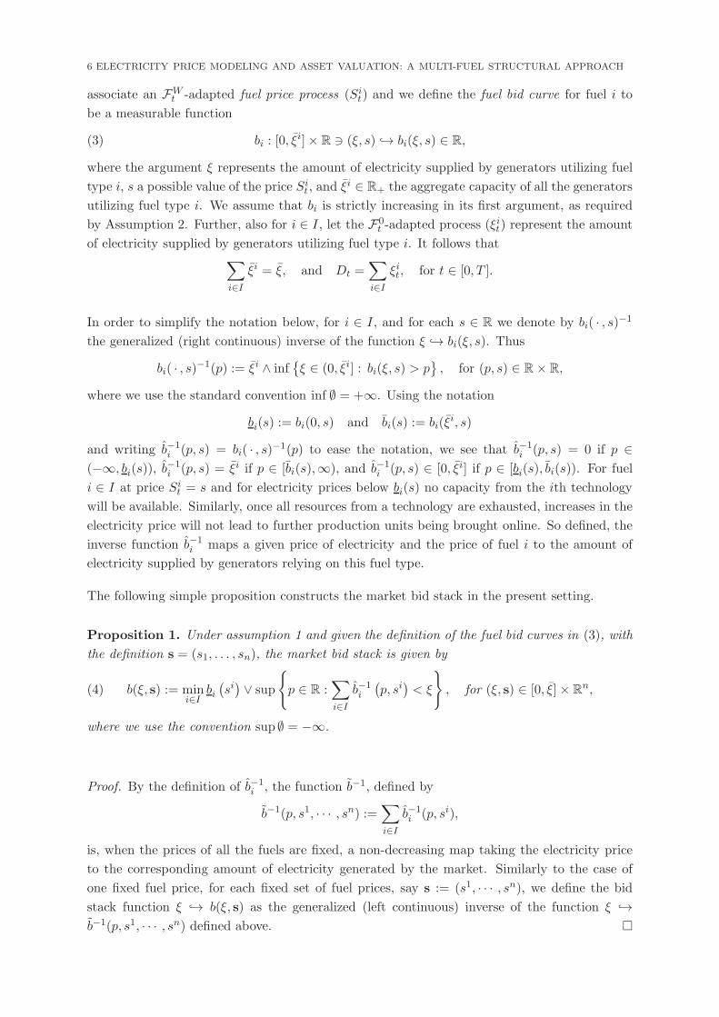

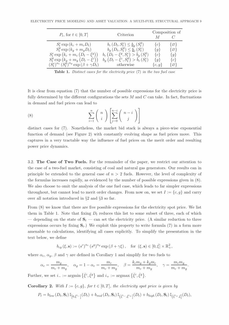
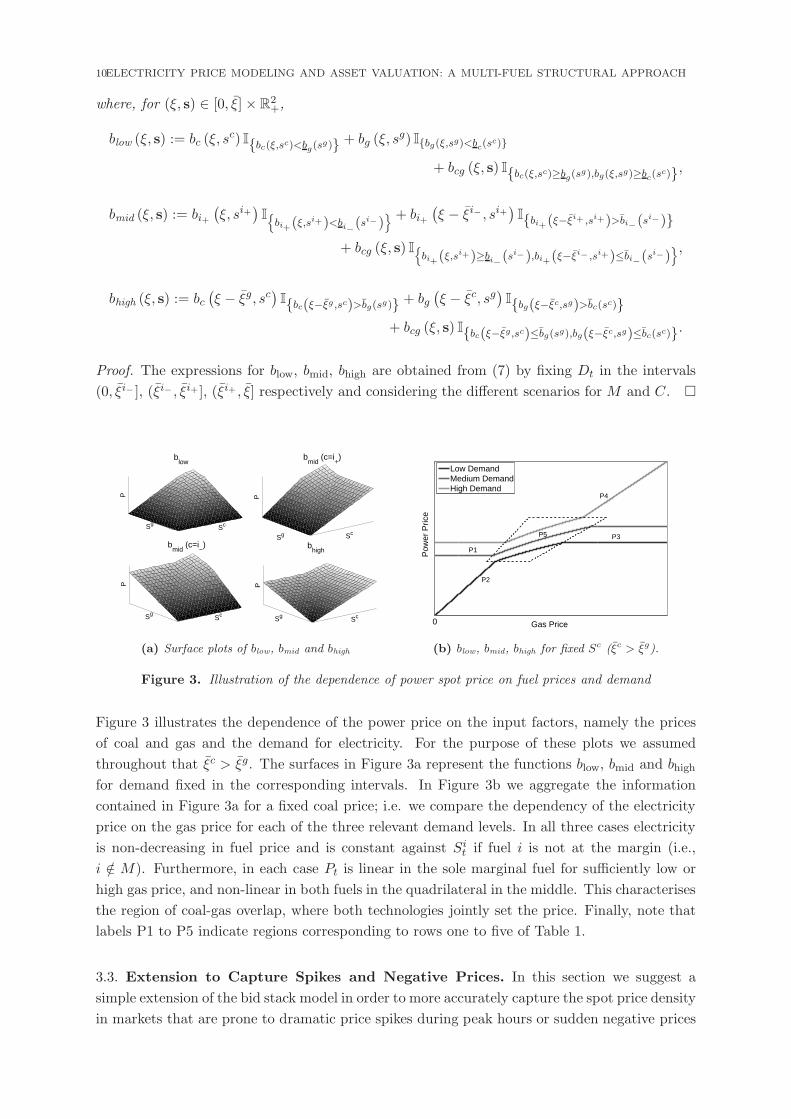

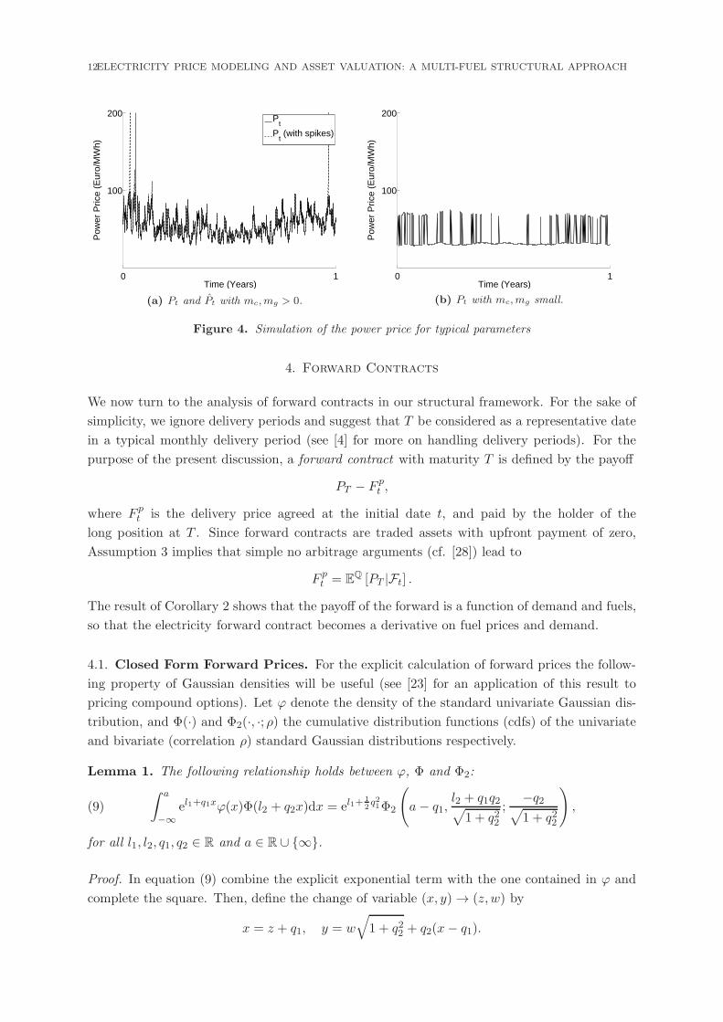


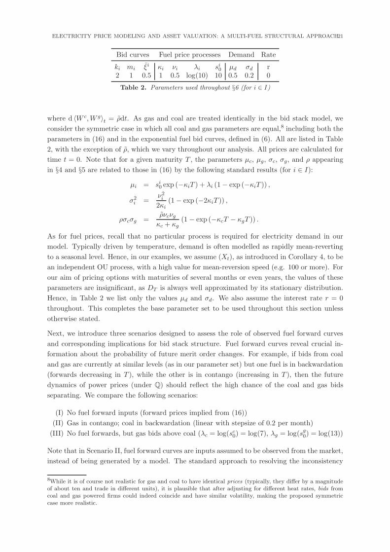
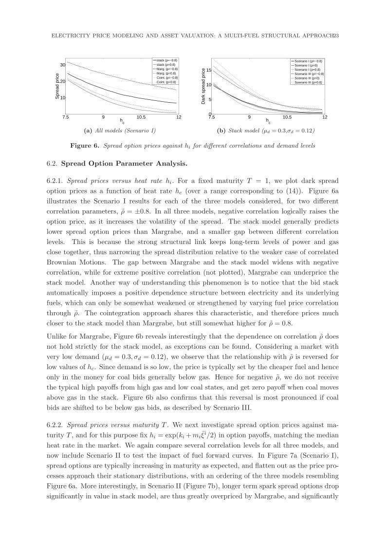


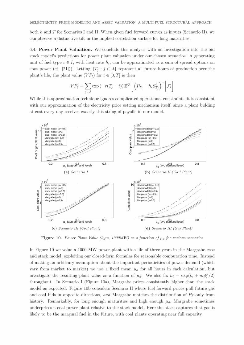
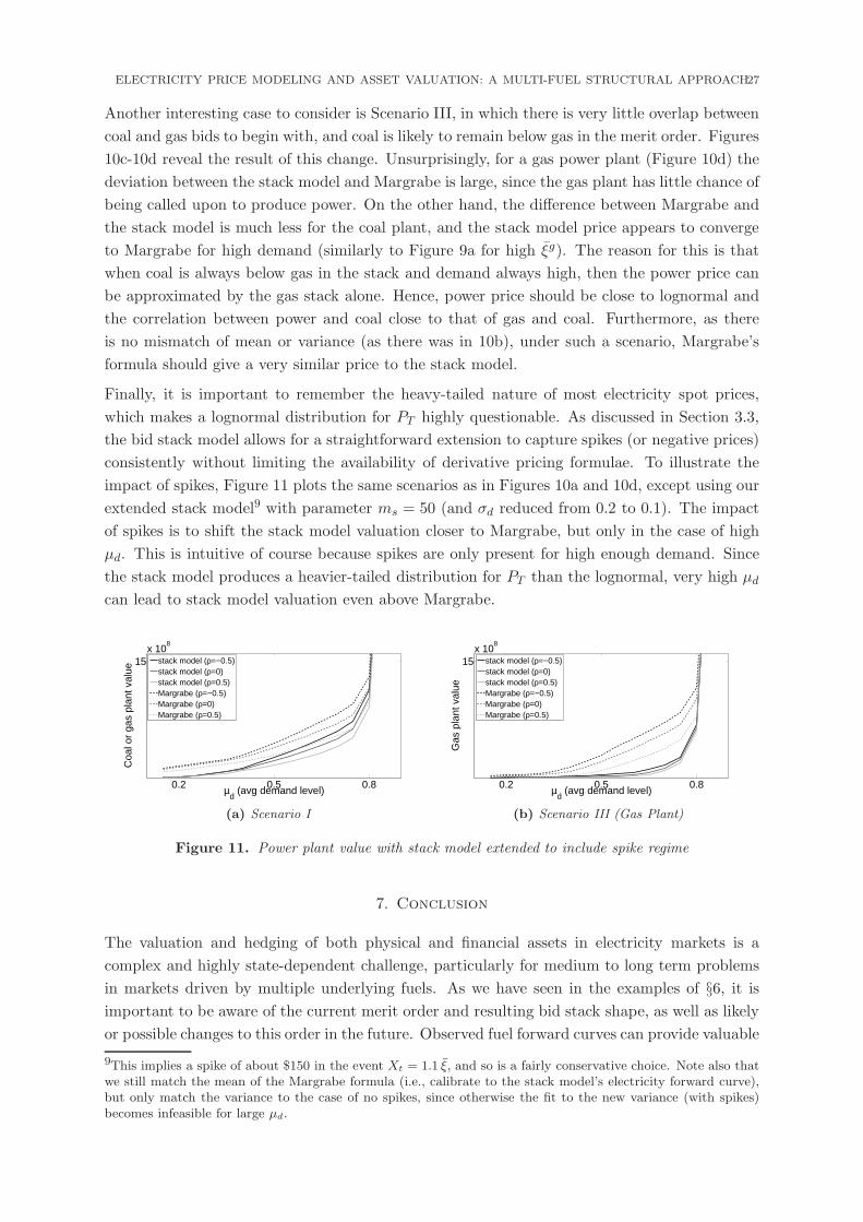


![ASSET Valuation[1]](https://static.documents.pub/doc/80x56/577d27af1a28ab4e1ea48bd2/asset-valuation1.jpg)


