“Electricity Storage, Emissions Taxes, and the Dynamic Value of Intermittent Renewable Energy” 40 th IAEE INTERNATIONAL CONFERENCE June 20 th , 2017. Singapore Ph.D. (c) Miguel Castro Michigan State University [email protected]
Transcript
“Electricity Storage, Emissions Taxes, and the Dynamic Value of Intermittent Renewable Energy”
• What is the value of intermittent renewable energy (IRE) sources, such as wind and solar?• Reduce grid-level electricity generation costs and emissions.
• Cyclical and random intermittency—difficult to integrate them to electric grids
• Need to account for the dynamic interactions between storage capacity and emissions regulations in assessing the value of intermittent renewables.• Previous studies have explored:
• the costs of intermittency (Gowrisankaran et al, 2015),
• the impact of storage on generation and investment in generating capacity (De Sisternes et al., 2016),
• the value of wind generation in the presence of storage under market power (Sioshansi, 2011),
• the long-term dynamic effects of carbon taxes on electricity markets (Cullen and Reynolds, 2016).
Introduction
• This research explores the dynamic value of intermittent renewable energy contingent on storage and emissions taxes• Using a stylized Social Planner Dynamic model of the Texas (ERCOT) electricity market that
simulates allocations, welfare and emissions (CO2, NOx, and SO2) for different storage and renewable energy levels.
• Assessment of wind power values under different scenarios combining storage availability and emissions taxes
• Storage capacity and emissions taxes are complements in driving the value of wind.
• Energy is allocated when it is most socially valuable.
• Wind power first best value doubles its LCOE but second best does not.
• Storage first best value (economic welfare) covers its cost but a second best does not
• Simply taxing emissions leads to a larger welfare gain than planned storage (324 MW) in ERCOT.
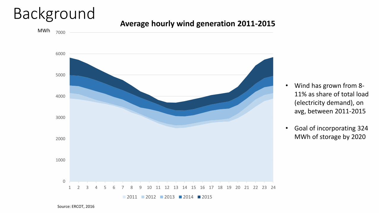
• Wind has grown from 8-11% as share of total load (electricity demand), on avg, between 2011-2015
• Goal of incorporating 324 MWh of storage by 2020
Average hourly load and wind generation in Texas for 2015
Storage helps smoothing demand and wind power cycles
Substitution of off-peak, high-carbon coal generation for on-peak, low-carbon natural gas generation. Carson and Novan (2013)
Cycles of wind power and storage dynamics
Empirical Model.
• Calibrate demand, marginal private and social costs using hourly data on load, generation, heat rate and emissions from EPA-CEMs, EIA and ERCOT. Marginal dmg estimates from social cost of carbon (US IAWG, 2015), SO2 and NOx smoke stack emissions (Muller and Mendehlson, 2009)
• Draw rip from hourly wind power deciles uniform distribution and solve the maximization problem with CONOPT. (1000 draws)
• Simulate the heterogeneous generation effects of an increase in wind power capacity with decile regressions
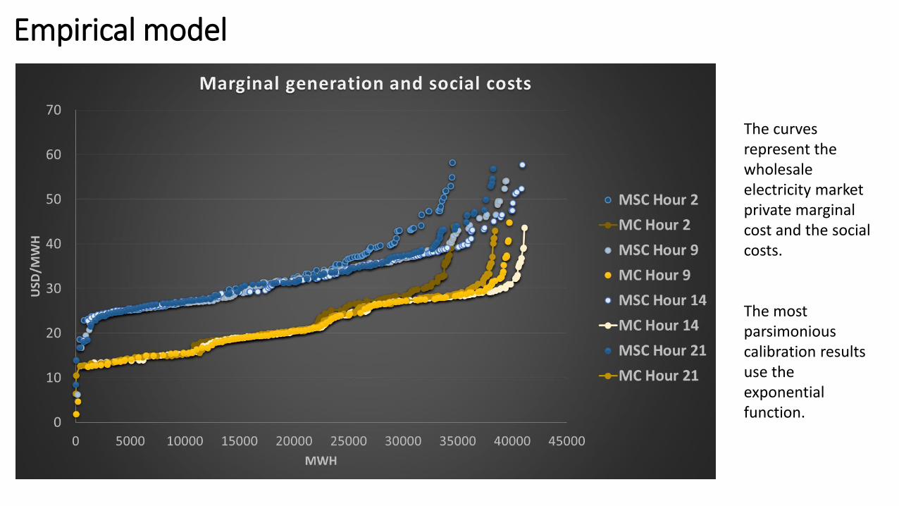
The curves represent the wholesale electricity market private marginal cost and the social costs.
The most parsimonious calibration results use the exponential function.
Compute the marginal value of increasing wind power and storage under different emissions taxes and storage scenarios
Empirical Model.
1. No storage, no tax (baseline) 𝑣𝑜(𝑟𝑡) 3. Storage, no tax 𝑣2(𝑟𝑡)2. No storage, tax on all emissions 𝑣1(𝑟𝑡) 4. Storage, tax on all emissions 𝑣3(𝑟𝑡)
No tax With tax
Value of wind 𝐸
𝑣𝑜(𝑟𝑡 + ∆𝑟𝑡) − 𝑣𝑜(𝑟𝑡)
∆𝑟𝑡 𝐸
𝑣1(𝑟𝑡 + ∆𝑟𝑡) − 𝑣𝑜(𝑟𝑡)
∆𝑟𝑡
Value of wind with storage 𝐸
𝑣2(𝑟𝑡 + ∆𝑟𝑡) − 𝑣2(𝑟𝑡)
∆𝑟𝑡 𝐸
𝑣3(𝑟𝑡 + ∆𝑟𝑡) − 𝑣2(𝑟𝑡)
∆𝑟𝑡
Value of storage 𝐸
𝑣2(𝑟𝑡 + ∆𝑠𝑡𝑜) − 𝑣𝑜(𝑟𝑡)
∆𝑠𝑡𝑜𝑟𝑎𝑔𝑒 𝐸
𝑣3(𝑟𝑡 + ∆𝑠𝑡𝑜) − 𝑣1(𝑟𝑡)
∆𝑠𝑡𝑜𝑟𝑎𝑔𝑒
Preliminary results
Levying emissions taxes decreases power arbitraging of coal offpeak power for natural gas peak power.
For 2015 wind power generation (11% of Load) and demand levels, the ideal storage/arbitrage is around 700 MWh more than double the oficial 2020 planned levels(324 GWh).
Ideal storage and arbitrage (700 MWh) in the day
No emissions taxwith emissions tax
No emissions taxwith emissions tax
Arbitrage actions with ERCOT 324 MWh planned storage
Preliminary results
Storage alone slightly increases the value of intermittent renewables (1.66 USD/MWh avg)
The largest increase in value comes from correcting the emissions externalities when allocating power.
Wind power first best value (165 USD/MWh) doubles its LCOE but second best does not(40 USD/MWh)
Estimates consider the benefits of avoided fossil generation cost, emissions offsets and arbitrage.
Economic Value of Wind Power
LCOE wind 50 USD/MWh
External benefits wind Novan AEJ (2015): 27.5 USD/MWh
External benefits wind Kaffine et al (2013): 22 USD/MWh
USD/MWh
Preliminary results
Storage first best value (USD/kWh 472.91) covers its cost but a second best (adoptiongstorage without emissions taxes) does not (USD/kWh 15).
The second best value is low due to the damages from substituting peak gas generation with off peak coal excessively when we don’t take into account their emissions externalities.
First Best Economic Value of Storage
USD/kWh
MWh
Cost of investment 10 yr Tesla powerwall USD/kWh 442.86
Theoretical framework. Set up results to explain main findings. Complementarity storage and taxes.Why largest value increase with tax? 4 times!Tax, reduction arbitrage free level,Increase emissions?
Social Merit order reordering plants show color in curves
Graph bar 12-24 bins storage. Wave curves with std. error bandsTax reduces need for storage, avoid coal arbitrage but complements in value IRE
Value IRE curve 11-15-20-25%. Compare only external benefits Novan
Increase value IRE and storage not enough to cover inv. Costs yet? Dispatch and carbon structure Texas. Compare to value only emissions Novan
Storage modelling mainly deals with smoothing daily cycles not short term randomness.Finding emissions? No carbon tax, storage.
Next steps? Operation reserves, Markov switching?
Preliminary results
LCOE wind (50 USD/MWh)
USD/MWh
MWh
Graph6. Fossil generation and ideal storage allocation by period of the day
In the scenarios with storage, all fossil generation tends to converge to the same level throughout the day (arbitraging of prices)
For 2015 wind power levels (11% of Load) the ideal storage/arbitrage levels range between6.600 and 6.681 MW, on average, for the scenarios with and without tax respectively.
Levying emissions taxes decreases the optimal storage
Storage slightly increases the value of IRE (0.5-2 USD/MWh) The largest increase in value is due to correcting for the emissions externality when allocating generation.
Proposed next steps• Develop a new scenario with a tax on CO2 only and not on local pollutants.
• Assess arbitrage levels and mg values of IRE and storage for different wind integration (12%-30% range, intervals of 5%) and storage adoption levels (324 MW-6600MW).
• Model more detailed time granularity of arbitrage decisions (12 or 24 bins within a day). Sensitivity analysis
elasticity of D.
• Incorporate operation reserves requirements in order to capture the increasing costs of wind power intermittency
Use a time series unsupervised clustering methodology (Hidden Markov Models and Markov switching with 2015 data) to implement a detailed (realistic) simulation of the time horizon of the dynamic programming and value of wind power and storage.
Preliminary results
No emissions taxwith emissions tax
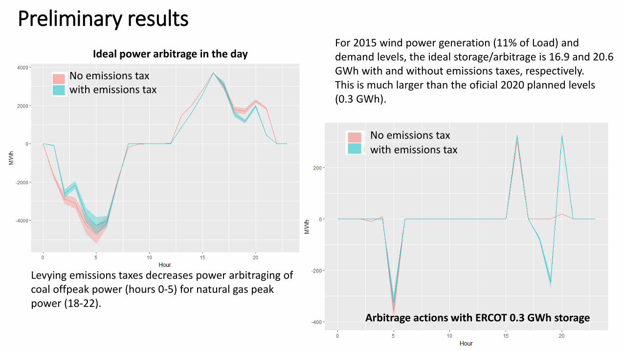
Levying emissions taxes decreases power arbitraging of coal offpeak power (hours 0-5) for natural gas peak power (18-22).
For 2015 wind power generation (11% of Load) and demand levels, the ideal storage/arbitrage is 16.9 and 20.6 GWh with and without emissions taxes, respectively. This is much larger than the oficial 2020 planned levels(0.3 GWh).
No emissions taxwith emissions tax
Ideal power arbitrage in the day
Arbitrage actions with ERCOT 0.3 GWh storage
Data and methods
WG. Wind generation explained by Wind Capacity WC plus hour and day effects. Different decile regressions for each period.
• Wind has grown from 8-12% as share of total load (electricity demand), on avg, between 2011-2015
• Goal of incorporating 324 MW of storage by 2020
Average hourly load and wind generation in Texas for 2015
Substitution of off-peak, high-carbon coal generation for on-peak, low-carbon natural gas generation
Theoretical model of IRE and storage.
ℎ𝑡<0 (recharge), 𝜏 marginal damage of emissions 𝑒𝑡(𝑓𝑡)IRE is a stochastic function of capacity 𝑟𝑡 = 𝑟𝑡(𝐶𝑎𝑝)
Assume two periods (offpeak and then peak). Peak demand is larger but there is more IRE generation at the offpeak.EXPLAIN ALL VARIABLES ABOVE!!No constraints on storage/ideal arbitrage. Using backward induction, total welfare is:
𝑣𝑜∗(𝑠𝑡 , 𝑟𝑡) = 𝑃𝑜(𝑓𝑜
∗(𝐶𝑎𝑝, 𝜂) + 𝑟𝑜 + ℎ𝑜∗(𝐶𝑎𝑝, 𝜂))𝑑𝑞
𝑄𝑖
0
− 𝐶𝑜(𝑓𝑜∗(𝐶𝑎𝑝, 𝜂)) − 𝜏𝑒𝑜(𝑓𝑜
∗(𝐶𝑎𝑝, 𝜂))
+ 𝛽𝐸𝑜 𝑃𝑝 𝑓𝑝∗(𝐶𝑎𝑝, 𝜂) + 𝑟𝑝 − 𝜂ℎ𝑜
∗(𝐶𝑎𝑝, 𝜂) 𝑑𝑞𝑄𝑖
0
− 𝐶𝑝 𝑓𝑝∗(𝐶𝑎𝑝, 𝜂) − 𝜏𝑒𝑝(𝑓𝑝
∗(𝐶𝑎𝑝, 𝜂))
𝜕𝑣𝑜(𝑟𝑡)
𝜕𝐶𝑎𝑝=
𝜕ℎ𝑜∗
𝜕𝐶𝑎𝑝(𝑃𝑜(∗)(1 − 𝜂)) +
𝜕𝑟𝑜𝜕𝐶𝑎𝑝
𝑃𝑜(∗) + 𝛽𝜕𝑟𝑝
𝜕𝐶𝑎𝑝𝑃𝑝(∗)
Assuming no uncertainty the value of IRE is given by:
Adding IRE capacity increases net welfare as long as the marginal value of generation increases overcomes storage losses
𝑀𝑎𝑥𝒇,𝒉 = 𝐸𝑜 𝛽𝑡 𝑃𝑡(𝑓𝑡 + 𝑟𝑡(𝐶𝑎𝑝) + ℎ𝑡)𝑑𝑞𝑄𝑖
0
− 𝐶𝑡(𝑓𝑡) − 𝜏𝑒𝑡(𝑓𝑡)
𝑇
𝑡=0
s.t: 𝑠𝑡+1 = 𝜂𝑠𝑡 − ℎ𝑡
𝑠𝑡 ≥ 0
Source: MIT Technology Review. Jan. 30th 2017Source: The Guardian. Aug. 25th, 2016
Source: The Guardian. Aug. 25th, 2016
• Introduction
• What is the value of intermittent renewable energy (IRE) sources, such as wind and solar? • Reduce grid-level electricity generation costs and emissions. • Cyclical and random intermittency—difficult to integrate them to electric grids (Joskow, 2011;
Baker et al., 2013). 15-18 minutes
• Assess the value of intermittent renewables by developing a stylized, welfare-maximizing dynamic model of the Texas (ERCOT) electricity market. • Previous studies (Sioshansi, 2011; Carson and Novan, 2013; Gowrisankaran et al, 2015; Cullen and
Reynolds, 2016; De Sisternes et al., 2016) have not accounted for the dynamic interactions between storage capacity and emissions regulations in assessing the effect of intermittent renewables on welfare.
• Storage capacity and emissions taxes are complements in driving the value of wind. • Compute the ideal storage-arbitrage levels for ERCOT• Adopting large levels of storage, even with emissions taxes, can lead to an increase in
pollution due to the substitution of off-peak, high-carbon coal generation for on-peak, low-carbon natural gas generation
Simulate the effects of electricity storage and environmental taxes on generation, emissions, and the value of wind generation.
Dynamic model of electricity generation and emissions
Renewable energy is modelled as a cyclic stochastic process (iid) with recurring realizations every day for each period t.
Using the Bellman equation (assumer linear Demand and Costs):
𝑣(𝑠𝑡 , 𝑟𝑡) = 𝑚𝑎𝑥𝑓 ,𝑠 𝑃𝑡 𝑓𝑡 + 𝑟𝑡 + ℎ𝑡 𝑑𝑞𝑄𝑖
0− 𝐶𝑡 𝑓𝑡 + 𝛽𝐸𝑡(𝑣(𝑠𝑡+1, 𝑟𝑡+1) 𝑡 )
Where: 𝑓𝑡 fossil fuel, ℎ𝑡 storage action level, Intermittent renewable energy 𝑟𝑡Assuming no losses, total load is 𝑄𝑡 = 𝑓𝑡 + 𝑟𝑡 + ℎ𝑡
Data and methodsThe curves represent the wholesale electricity market private marginal cost and the social costs.
The scheduler job is to dispatch plants according to the merit order based on private and social costs.
The most parsimonious calibration results use the exponential function. R2 >0.98
4 time periods of the day (0-5, 6-11, 12-17, 18-23).
Data and methods
Grid level CO2 Emissions with private MC dispatch EPA and EIA hourly data for2015 (8760 observationsfor 136 power plants)
Marginal damages:*social cost of carbon (USIAWG, 2015),*SO2 and NOx smoke stackemissions (Muller andMendehlson, 2009)
I calibrate the MarginalSocial Cost of electricitygeneration for thewholesale market usinghourly plant levelemissions
Data and methods
𝐷𝑒𝑐𝑖𝑙𝑒𝜏(𝑊𝐺𝑖 𝑿𝒊) = 𝛼(𝜏) + 𝑊𝐶𝑖𝛽1(𝜏) + 𝐻𝑜𝑢𝑟𝛽2(𝜏) + 𝐷𝑎𝑦𝛽3(𝜏) WG. Wind generation explained by Wind Capacity WC plus hour and day effects. Different decile regressions for each period.
Simulations and intended results
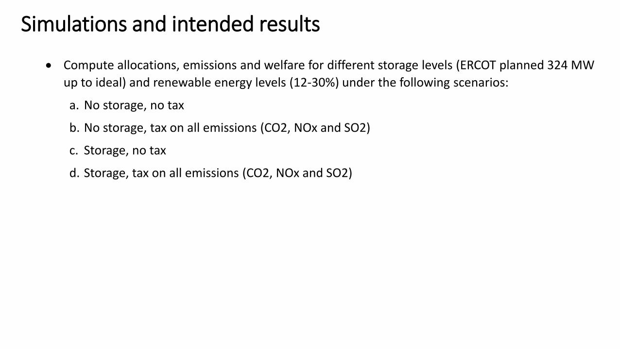
Compute allocations, emissions and welfare for different storage levels (ERCOT planned 324 MW
up to ideal) and renewable energy levels (12-30%) under the following scenarios:
a. No storage, no tax
b. No storage, tax on all emissions (CO2, NOx and SO2)
c. Storage, no tax
d. Storage, tax on all emissions (CO2, NOx and SO2)
Monte Carlo simulation implementation*Assume all information on wind generation is revealed at the start of the day*For each random draw (i), based on wind power decilesfor each representative hour, solve the maximization problem with GAMS-CONOPT* 1000 random draws
𝑟𝑖~𝑖𝑖𝑑(𝑛𝑖 , 𝜎𝑖2)
𝑠𝑡 ≤ 𝑠𝑚𝑎𝑥
No storage scenarios
• Find optimal expected fossil gen 𝐸(𝑓𝑖∗) and welfare
in the case of the model with MSC 𝐸(𝑊𝑖∗).
• For the model with no emissions taxes the optimization renders the surplus S* and we compute welfare subtracting the externality:
𝐸 𝑊𝑖∗ = 𝐸 𝑆𝑖
∗ − (𝑀𝑆𝐶 𝑓𝑖∗ − 𝑀𝐶 𝑓𝑖
∗
• Compute emissions using the polynomial fn. 𝐸(𝐸𝑚𝑖 𝑓𝑖
∗ )
Storage scenarios
• For the case of ideal storage, solve the maximization problem without any constraint on si. For the ERCOT planned storage, constrain 𝑠𝑖 ≤ 324
Preliminary resultsFossil generation and ideal storage allocation by period of the day
In the scenarios with storage, all fossil generation tends to converge to the same level throughout the day (arbitraging of prices)
For 2015 wind power levels (11% of Load) the ideal storage/arbitrage levels range between6.600 and 6.681 MW, on average, for the scenarios with and without tax respectively.
Levying emissions taxes decreases the optimal storage
Graph 24, 12 bars charging action, curve value IRE
Preliminary resultsIn 2015, the full economic value of wind power was around 140 USD/MWh(current situation with neither storage nor tax).
Adding emissions taxes triples the value of wind capacity and generation
Adding ideal storage means a six fold increase and combining storage and taxes yields a nine fold increase.
Need to consider operation reserve costs
Dynamic value of daily wind power capacity (MW) and generation (MWh)
Simulate the effects of electricity storage and environmental taxes on generation, emissions, and the value of wind generation.
Dynamic model of electricity generation and emissions
At the interior solution:
Optimal fossil fuel condition: 𝑃𝑡(𝑛𝑡𝐹𝐹 + 𝑛𝑡
𝑅𝐸 + ℎ𝑡) ≤ 𝐶′(𝑛𝑡𝐹𝐹)
And arbitrage
𝑃𝑡(𝑛𝑡𝐹𝐹 + 𝑛𝑡
𝑅𝐸 + ℎ𝑡) ≤ 𝛽𝐸𝑡(𝑃𝑡+1(𝑛𝑡+1𝐹𝐹 + 𝑛𝑡+1
𝑅𝐸 + ℎ𝑡+1) 𝑡 𝜖 𝑝𝑒𝑎𝑘, 𝑜𝑓𝑓𝑝𝑒𝑎𝑘 )
Renewable energy is modelled as a cyclic stochastic process (iid) with recurring realizations every day for each period t.
Using the Bellman equation (assumer linear Demand and Costs):
𝑣(𝑠𝑡 , 𝑟𝑡) = 𝑚𝑎𝑥𝑓 ,𝑠 𝑃𝑡 𝑓𝑡 + 𝑟𝑡 + ℎ𝑡 𝑑𝑞𝑄𝑖
0− 𝐶𝑡 𝑓𝑡 + 𝛽𝐸𝑡(𝑣(𝑠𝑡+1, 𝑟𝑡+1) 𝑡 )
Where: 𝑓𝑡 fossil fuel, ℎ𝑡 storage action level, Intermittent renewable energy 𝑟𝑡Assuming no losses, total load is 𝑄𝑡 = 𝑓𝑡 + 𝑟𝑡 + ℎ𝑡
St is the storage level
𝑀𝑎𝑥𝒇,𝒉 = 𝐸𝑜 𝛽𝑡 𝑃𝑡(𝑓𝑡 + 𝑟𝑡 + ℎ𝑡)𝑑𝑞𝑄𝑖
0
− 𝐶𝑡(𝑓𝑡)
𝑇
𝑡=0
s.t: 𝑠𝑡+1 = 𝜂𝑠𝑡 − ℎ𝑡
𝑠𝑡 ≥ 0
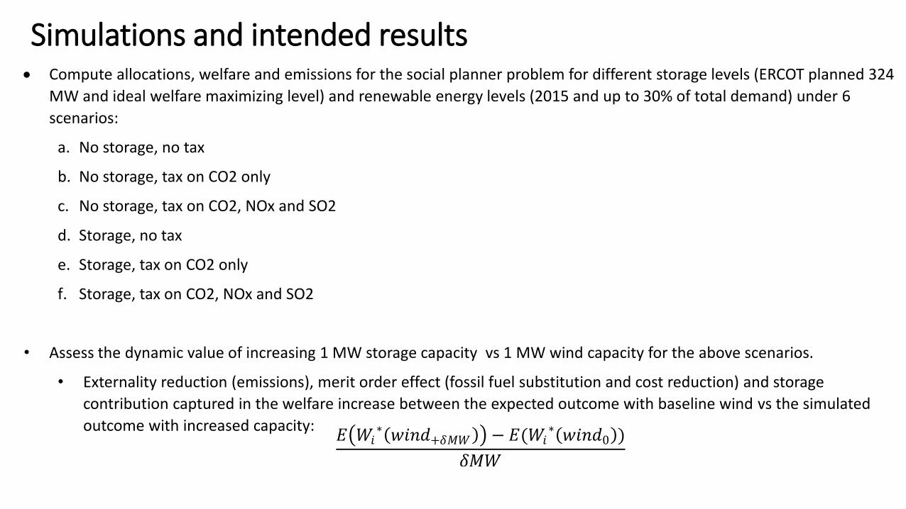
Simulations and intended results Compute allocations, welfare and emissions for the social planner problem for different storage levels (ERCOT planned 324
MW and ideal welfare maximizing level) and renewable energy levels (2015 and up to 30% of total demand) under 6
scenarios:
a. No storage, no tax
b. No storage, tax on CO2 only
c. No storage, tax on CO2, NOx and SO2
d. Storage, no tax
e. Storage, tax on CO2 only
f. Storage, tax on CO2, NOx and SO2
• Assess the dynamic value of increasing 1 MW storage capacity vs 1 MW wind capacity for the above scenarios.
• Externality reduction (emissions), merit order effect (fossil fuel substitution and cost reduction) and storage
contribution captured in the welfare increase between the expected outcome with baseline wind vs the simulated
outcome with increased capacity:𝐸 𝑊𝑖
∗(𝑤𝑖𝑛𝑑+𝛿𝑀𝑊) − 𝐸(𝑊𝑖∗(𝑤𝑖𝑛𝑑0))
𝛿𝑀𝑊
Data and methods: MC simulation for dynamic value of wind
*For each random draw (i), based on wind power deciles for each representative hour, solve the maximization problem with GAMS-CONOPT𝑟𝑖~𝑖𝑖𝑑(𝑛𝑖 , 𝜎𝑖
2) 𝑠𝑡 ≤ 𝑠𝑚𝑎𝑥
No storage scenarios
• Find optimal expected fossil gen 𝐸(𝑓𝑖∗) and welfare
in the case of the model with MSC 𝐸(𝑊𝑖∗).
• For the model with no emissions taxes the optimization renders the surplus S* and we compute welfare subtracting the externality:
𝐸 𝑊𝑖∗ = 𝐸 𝑆𝑖
∗ − (𝑀𝑆𝐶 𝑓𝑖∗ − 𝑀𝐶 𝑓𝑖
∗
• Compute emissions using the polynomial fn. 𝐸(𝐸𝑚𝑖 𝑓𝑖
∗ )
Storage scenarios
• For the case of ideal storage, solve the maximization problem without any constraint on si. For the ERCOT planned storage, constrain 𝑠𝑖 ≤ 324
Implementing storage and emissions taxes lead to the most efficient outcome by properly accounting for the externality related deadweight loss and for the flexibility in allocating energy when it is most valuable.
Preliminary resultsFossil generation and 324 MW of storage allocation by period of the day
With constrained storage we see a smaller reduction in fossil generation.
Preliminary resultsAdding a tax decreases all emissions in all scenarios.
Ideal storage scenariosHaving storage in addition to emissions taxes increases all emissions slightly since the benefits of arbitraging electricity compensate for the externality damages caused by substituting peak gas generation with base coal generation.
Only NOx emissions increase in the scenario with storage compared to the current baseline. Arbitraging coal for gas steam turbines (large Noxemissions factor, 1.6 lbs/MWh).
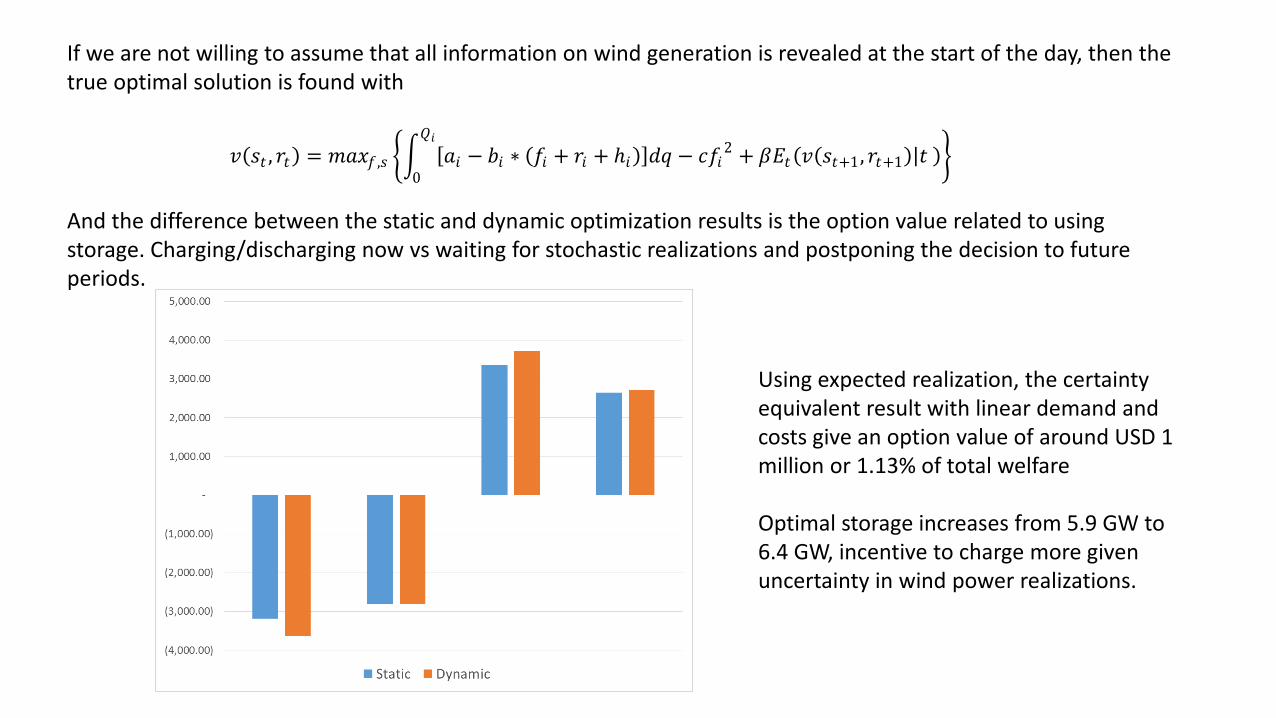
If we are not willing to assume that all information on wind generation is revealed at the start of the day, then the true optimal solution is found with
And the difference between the static and dynamic optimization results is the option value related to using storage. Charging/discharging now vs waiting for stochastic realizations and postponing the decision to future periods.
Using expected realization, the certainty equivalent result with linear demand and costs give an option value of around USD 1 million or 1.13% of total welfare
Optimal storage increases from 5.9 GW to 6.4 GW, incentive to charge more given uncertainty in wind power realizations.
Next steps
• Run several simulations with incremental levels of storage (from 0 to ideal) to plot the value of wind power for different wind integration levels (12%-30% range)
• Constraint on borrowing electricity throughout time! In option value solution
• Why with iid is there an option value?!
• Incorporate operation reserves cost to add detail on the increasing costs wind power intermittency• Startup and ramping costs, coal power plants might change Marginal Cost Curve (Dr. Herriges, argument)
• Run Monte Carlo simulations for wind power realizations with the dynamic solution (option value) for ideal storage levels.
• Texas electricity grid and market (ERCOT) >1% hydropower, and marginal imports
• Wind has grown from 8-12% share of total load, on avg, between 2011-2015
• Ideal case study to simulate effects of future storage
• Goal of incorporating 324 MW of storage by 2020
• Emerging initiatives and technologies for storage
• SHOW LOAD IN GRAPH, INTUITION, HIGHER LOAD PEAK AND LESS WIND.
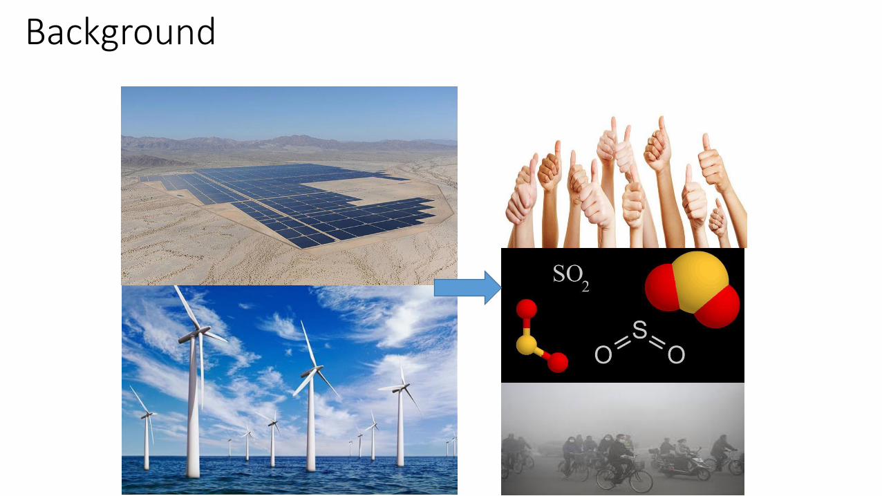
- An electric grid powered primarily by renewable energy is one of the proposed alternatives for reducing air pollution and GHG.
- There are some encouraging efforts:
* Several state level renewable portfolio standard policies RPS and feed in tariff schemes
* CAISO goal of integrating 33% RE generation by 2020
Evolution of solar and wind generation in the CAISO grid 2011-2015
Solar went from 1% to 7% and wind from 3% to 6% between 2011-2015 in California
Source: Data extracted from CAISO online webpage
Literature review
• Short run benefits of IRE: displaced generation (merit order effect) and emissions.
• Benefits reduced by intermittency of wind and solar power—both cyclical and random—can make it difficult to integrate these sources into conventional electric grids (Joskow, 2011; Baker et al., 2013).
• Storage can ease IRE integration and increase the benefits but it could also lead to an increase in total CO2 emissions, by facilitating the substitution of off-peak, high-carbon coal generation for on-peak, low-carbon natural gas generation (Carson and Novan, 2013).
Literature review
• Previous literature:• costs of intermittency (Gowrisankaran et al, 2016),
• the impact of storage on generation and investment in generating capacity (De Sisternes et al., 2016),
• the value of wind generation in the presence of storage under market power (Sioshansi, 2011),
• and the long-term dynamic effects of carbon taxes on electricity markets (Cullen and Reynolds, 2016).
• Need to account for the interactions between storage capacity and emissions regulations in assessing the performance of intermittent renewables.
Static version of dynamic intraday storage problem
𝑟𝑖~𝑖𝑖𝑑(𝑛𝑖 , 𝜎𝑖2)
𝑠𝑡 ≤ 𝑠𝑚𝑎𝑥
Optimal solution is repetition of daily static solution
If we are willing to assume that all information on wind generation is revealed at the start of the day, we get:
𝑀𝑎𝑥𝒇,𝒔 = 𝐸𝑜 𝛽𝑡 𝑃𝑖(𝑓𝑖 + 𝑟𝑖 + 𝑠𝑖)𝑑𝑎𝑄𝑖
024
− 𝐶(𝑓𝑖)
24
𝑇
𝑡=0
s.t: 𝑠𝑖4 = 0 (storage lasts no longer than a day)
In the case of constrained storage
Using the demand bins, I obtain the deciles of wind power generation for each period in day based on 2015 data.
These deciles are used in a Monte Carlo simulation aimed at finding the expected welfare and allocations of 1000 random draws.
In order to simulate the differentiated impact of increasing wind capacity on generation throughout the day, I use decile regressions of wind power generation on installed capacity:
Data and methods
𝑣(𝑠1, 𝑟1)
= 𝑚𝑎𝑥𝑓 ,ℎ
𝑎1 − 𝑏1 ∗ (𝑓1 + 𝑟1 + ℎ1) 𝑑𝑞𝑄𝑖
0
− 𝑐𝑓12
+ 𝛽𝐸𝑡
𝑎2(𝑓2 + 𝑟2 + ℎ2) −
𝑏22 ∗ 𝑓2 + 𝑟2 + ℎ2(𝑠2, 𝑟2)
2− 𝑐
𝑎2 − 𝑏2 ∗ 𝑟2 + ℎ2(𝑠2, 𝑟2) 2𝑐 + 𝑏2
2
+
𝛽𝐸𝑡
𝑎𝑇 𝑎𝑇 + 2𝑐 ∗ 𝑟𝑇 + 𝑠2 − 𝜂ℎ2(𝑠2, 𝑟2)
2𝑐 + 𝑏𝑇 −
𝑏𝑇2 ∗
𝑎𝑇 + 2𝑐 ∗ 𝑟𝑇 + 𝑠2 − 𝜂ℎ2(𝑠2, 𝑟2) 2𝑐 + 𝑏𝑇
2
− 𝑎𝑇 − 𝑏𝑇 ∗ 𝑟𝑇 + 𝑠2 − 𝜂ℎ2(𝑠2, 𝑟2)
2𝑐 + 𝑏𝑇
2
𝑡 = 2
𝑡 = 1
For example at the second period, the value function looks like:
We solve all the way to the first period and we will find the optimal allocations and welfare (value function at initial time period).
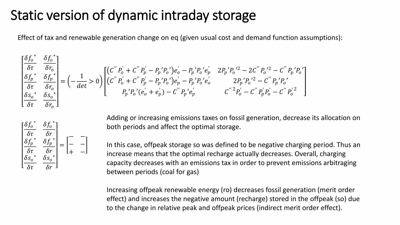
Effect of tax and renewable generation change on eq (given usual cost and demand function assumptions):
𝛿𝑓𝑜
∗
𝛿𝜏
𝛿𝑓𝑜∗
𝛿𝑟𝑜𝛿𝑓𝑝
∗
𝛿𝜏
𝛿𝑓𝑝∗
𝛿𝑟𝑜𝛿𝑠𝑜
∗
𝛿𝜏
𝛿𝑠𝑜∗
𝛿𝑟𝑜
= −1
𝑑𝑒𝑡> 0
𝐶′′ 𝑃𝑜′ + 𝐶′′ 𝑃𝑝
′ − 𝑃𝑝 ′𝑃𝑜 ′ 𝑒𝑜′ − 𝑃𝑝 ′𝑃𝑜 ′𝑒𝑝
′ 2𝑃𝑝 ′𝑃𝑜 ′2 − 2𝐶′′ 𝑃𝑜 ′
2 − 𝐶′′ 𝑃𝑝 ′𝑃𝑜 ′
𝐶′′ 𝑃𝑜′ + 𝐶′′ 𝑃𝑝
′ − 𝑃𝑝 ′𝑃𝑜 ′ 𝑒𝑝′ − 𝑃𝑝 ′𝑃𝑜 ′𝑒𝑜
′ 2𝑃𝑝 ′𝑃𝑜 ′2 − 𝐶′′ 𝑃𝑝 ′𝑃𝑜 ′
𝑃𝑝 ′𝑃𝑜 ′(𝑒𝑜′ + 𝑒𝑝
′ ) − 𝐶′′ 𝑃𝑝 ′𝑒𝑝′ 𝐶′′ 2
𝑃𝑜′ − 𝐶′′ 𝑃𝑝
′𝑃𝑜′ − 𝐶′′ 𝑃𝑜
′ 2
𝛿𝑓𝑜
∗
𝛿𝜏
𝛿𝑓𝑜∗
𝛿𝑟𝛿𝑓𝑝
∗
𝛿𝜏
𝛿𝑓𝑝∗
𝛿𝑟𝛿𝑠𝑜
∗
𝛿𝜏
𝛿𝑠𝑜∗
𝛿𝑟
=
− −− −+ −
Adding or increasing emissions taxes on fossil generation, decrease its allocation on both periods and affect the optimal storage.
In this case, offpeak storage so was defined to be negative charging period. Thus an increase means that the optimal recharge actually decreases. Overall, charging capacity decreases with an emissions tax in order to prevent emissions arbitraging between periods (coal for gas)
Increasing offpeak renewable energy (ro) decreases fossil generation (merit order effect) and increases the negative amount (recharge) stored in the offpeak (so) due to the change in relative peak and offpeak prices (indirect merit order effect).