Electro-osmotic flows through topographically complicated porous media:Role of electropermeability tensor
Aditya Bandopadhyay,1 Debabrata DasGupta,2 Sushanta K. Mitra,3 and Suman Chakraborty1,2,*
1Advanced Technology Development Center, Indian Institute of Technology Kharagpur, Kharagpur, India, 7213022Department of Mechanical Engineering, Indian Institute of Technology Kharagpur, Kharagpur, India, 721302
3Micro and Nano-scale Transport Laboratory, University of Alberta, Canada, T6G 2G8(Received 26 September 2012; revised manuscript received 15 January 2013; published 12 March 2013)
In the present work, we consider a framework for characterizing electro-osmotic flows in topographicallycomplicated porous media and derive an effective up-scaled transport parameter to quantify this. We term thisparameter the electro-permeability, which characterizes the electro-osmotic flow through composite porous mediain analogy with Darcy’s law. The electro-permeability tensor, thus introduced, serves a simple means of relatingthe volume flow rate with the applied electric field without going into the intricacies of the microstructureof the porous domain. First, we consider cases where the solid fractions have a fractal dimension generatedby the Mandelbrot set, purely for the sake of demonstration. Based on such considerations, we employ themethod of homogenization to obtain the effective electro-permeability parameter from the numerical simulationsexecuted over a representative volume element. Our derived electro-permeability tensor components exhibitfunctional relationships with the solid or liquid fraction as well as the topography of the porous medium. Havingestablished these functional relationships, we evaluate the tensor components for a binary composite porousmedium in which one constituent has markedly high ζ potential than the other constituent, for illustration withpotential relevance in microfluidics. We establish the sensitivity of the electro-permeability tensor on the domainmorphology, solid fraction, ratio of solid fractions of the two phases having the two different ζ potential values,and the ζ potential contrast and compare it with equivalent Darcy permeability for the same. We thus provide asimple mathematical framework that may be immensely helpful for devising a computationally efficient way ofcharacterizing electro-osmosis through topographically complicated porous media.
With increasing applications of flows through membranes(e.g., proton exchange membranes [1]), nanoporous media(for energy conversion [2–4]), and fibrous media (e.g., papermicrofluidics [5,6]), it is imperative to address the transportof colloids and aqueous solutions through a domain thatis characterized by a tortuous and highly networked path[7]. In the traditional paradigm of pressure-driven flowsthrough porous media, one typically refers to Darcy’s lawin addressing such scenarios, which relates the volume flowrate to the applied pressure gradient via the permeabilityparameter [8]. An inherent simplicity of Darcy’s law stemsfrom the fact that it may accommodate various correlations inorder to represent the consequences of inherent topographicalfeatures like porosity and tortuosity in the flow analysis.However, despite its inherent simplicity, use of it is oftenrestricted by its obvious limitations in explicitly capturingthe consequences of complicated topography of the domainfrom a rather fundamental perspective. The situation gets evenmore challenging when electro-osmosis occurs within the flowdomain, by virtue of an intricate interaction between a chargedinterfacial layer formed at the solid-liquid interface, alsoknown as the electrical double layer (EDL), and an externallyapplied electric field [9–22]. Implications of the topographyof the porous medium on the resultant flow characteristics,under such circumstances, may remain far from being trivial,
because of combined multiphysics and multiscale nature ofthe underlying transport processes.
In an analogy to Darcy’s law, here we develop an effectiveelectro-permeability parameter which would relate the volumeflow rate with the applied electric field for electro-osmotic flowin porous media. Electro-osmosis through porous media hasfound applications in areas like: soil dewatering, enhancedoil recovery in bitumen [23], proton exchange membranes infuel cells [1,24,25], flows involving suspensions of chargedparticles [26,27], and liquid transfers in soils [25]. As such,electro-osmotic transport in a porous medium is a complicatedinterplay of the EDL [23,29], the topographical feature of theflow domain, and the applied electric field, which may best beaddressed in a computationally efficient manner by employingthe concepts of multiple physical scales.
A wide variety of physical problems have multiple scalesintegrated into the physics of the problem. A few suchproblems are flows in porous media, turbulent flows, analysisof composite materials, and many more [30–36]. Usually theseproblems involve complex geometries or topographies andhence are quite often not analytically tractable. For example,flows of Newtonian fluids in porous media involve the solutionof the full Navier-Stokes equation in a complex domain. Thesituation may be further complicated by the fact that in orderto capture the underlying physics of the problem (for instance,flows through tortuous channels bearing surface potential),we are required to resolve the computational domain to thesmallest length scale so that the local fluctuations are captured.Failure to resolve the domain to the smallest domain of interestmay lead to physically unrealistic solutions because of theinability to capture the physics which has its genesis in the
BANDOPADHYAY, DASGUPTA, MITRA, AND CHAKRABORTY PHYSICAL REVIEW E 87, 033006 (2013)
1
2
3
4
5
fsΓ
fY
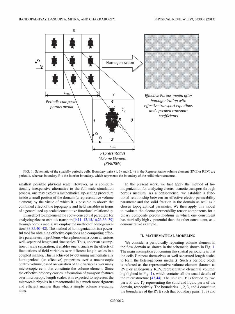
FIG. 1. Schematic of the spatially periodic cells. Boundary pairs (1, 3) and (2, 4) in the Representative volume element (RVE or REV) areperiodic, whereas boundary 5 is the interior boundary, which represents the boundary of the solid microstructure.
smallest possible physical scale. However, as a computa-tionally inexpensive alternative to the full-scale simulationprocess, one may exploit a mathematical up-scaling procedureinside a small portion of the domain (a representative volumeelement) by the virtue of which it is possible to absorb thecombined effect of the topography and field variables in termsof a generalized up-scaled constitutive functional relationship.
In an effort to implement the above conceptual paradigm foranalyzing electro-osmotic transport [9,11–13,15,16,23,36–39]through porous media, we employ the method of homogeniza-tion [33,35,40–42]. The method of homogenization is a power-ful tool for obtaining effective equations and computing effec-tive parameters in problems where phenomena occur at variouswell-separated length and time scales. Thus, under an assump-tion of scale separation, it enables one to analyze the effects offluctuations of field variables over different length scales in acoupled manner. This is achieved by obtaining mathematicallyhomogenized (or effective) properties over a macroscopiccontrol volume, based on variation of field variables over manymicroscopic cells that constitute the volume element. Sincethe effective property carries information of transport featuresover microscopic length scales, it is expected to represent themicroscale physics in a macromodel in a much more rigorousand efficient manner than what a simple volume averagingdoes.
In the present work, we first apply the method of ho-mogenization for analyzing electro-osmotic transport throughporous medium. As a consequence, we establish a func-tional relationship between an effective electro-permeabilityparameter and the solid fraction in the domain as well as achosen topographical parameter. We then apply this modelto evaluate the electro-permeability tensor components for abinary composite porous medium in which one constituenthas markedly high ζ potential than the other constituent, as ademonstrative example.
II. MATHEMATICAL MODELING
We consider a periodically repeating volume element inthe flow domain as shown in the schematic shown in Fig. 1.The main assumption concerning this spatial periodicity is thatthe cells Y repeat themselves at well-separated length scalesto form the heterogeneous media X. Such a periodic blockis referred as the representative volume element (known asRVE or analogously REV, representative elemental volume;highlighted in Fig. 1), which contains all the small details ofthe microstructure [43,44]. The unit cell Y is formed by twoparts Ys and Yf representing the solid and liquid parts of thedomain, respectively. The boundaries 1, 2, 3, and 4 constitutethe boundaries of the RVE such that boundary pairs (1, 3) and
033006-2
ELECTRO-OSMOTIC FLOWS THROUGH TOPOGRAPHICALLY . . . PHYSICAL REVIEW E 87, 033006 (2013)
(2, 4) are periodic and boundary 5, represented as �f s , is theinterface separating Ys and Yf .
Before introducing a formal implementation of the methodof homogenization as applied to the porous media in thecontext of electro-osmotic transport, we first mention the gov-erning equations for electrical potential distribution becauseof the presence of surface charges on the walls of the porousmedia, which is central to the phenomenon of electro-osmosis.
A. EDL potential distribution induced in the porous medium
The potential distribution (ψ) in the EDL is coupled with thecharge density distribution (ρe) through the Poisson equation,as given by [29]
∇2ψ = −ρe/εr , (1)
where
ρe = e(z+n+ + z−n−). (2)
Here εr is the permittivity of the media, e is the protonic charge,z+ and z− represent the valency of positive and negativelycharged species respectively, and n+ and n− represent theionic number densities of the positive and negative species,respectively. The ionic number densities are assumed to bedescribed by the Boltzmann distribution [29], which is givenas
n± = n0 exp(−z±eψ/kBT ), (3)
where n0 is the bulk ionic concentration, kB is the Boltzmannconstant, and T is the absolute temperature. For a z: z
symmetric electrolyte, Eqs. (1)–(3) can be combined togetherto yield the Poisson-Boltzmann equation [29]:
∇2ψ = 2zen0
εr
sinh
(zeψ
kBT
). (4)
Equation (4) is subjected to ζ potential at the shear plane(effectively the interface between the wall-adhering immobileionic layer and the outer mobile ionic layer; here applied atboundary 5 in Fig. 1) and periodic boundary conditions on theRVE/REV boundaries.
B. Hydrodynamic equations
The corresponding governing transport equations for asteady flow of Newtonian fluid are
�∇ · �v = 0, (5)
ρ�v · �∇�v = −�∇p + μ∇2�v + ρe�E. (6)
Equation (5) represents the continuity equation, and Eq. (6)represents the momentum equation with an augmented bodyforce term, which is derived from the Maxwell stress tensor[10]. Here �v is the flow velocity, p is the pressure, μ is theviscosity, and �E is the electrical field. Equation (6) is subjectto no slip and no flux at the solid boundaries bounding thetopographically complex domain present in each RVE/REV(boundary 5 in Fig. 1) and periodicity on the RVE/REVboundaries.
C. Applied potential field
In addition to the EDL potential field, an electric field dueto the externally applied voltage is also established. The latersatisfies the Laplace equation [29,45] as given by
∇2φ = 0. (7)
Equation (7) is subject to no electric flux on the solidboundaries bounding the topographically complex domainpresent in each RVE/REV (boundary 5 in Fig. 1), and Dirichletboundary conditions on two parallel boundaries (for example,boundaries 1 and 3 for an electric field applied along the x1
direction), and periodic on the other two of the RVE/REVboundaries (for example, boundaries 2 and 4 for an electricfield applied along the x1 direction).
D. Asymptotic expansion and homogenized equations
We nondimensionalize the governing equations andboundary conditions with the following parameters: xi =xi/Lmac, yi = yi/Lmic, ψ = ψ/ζ , φ = φ/φref , vi = vi/Uref ,Eref = φref/Lmac, and ∇p = ∇p/(∇p)ref where Uref =(εrζφref)/(Lmacμ), (∇p)ref = μUref/L
2mac where Lmac and Lmic
are the characteristic length scale of the macroscopic andmicroscopic domains respectively, εr is the permittivity ofthe medium, and ζ is the wall ζ potential.
If the number of microscopic periodically repeating unitcells constituting the macroscopic domain is small, the ratio ofthe characteristic micro to the macrolength scale, (Lmic/Lmac),is not small, and the assumption of the separation of scale fails.In such cases, the effective property is not an intrinsic one,and there is no effective description of the porous medium.Therefore, the fundamental requirement is that the scales mustbe separated such that the condition ε = Lmic/Lmac � 1 issatisfied. If the separation of scales is valid, any field quantitymay effectively be represented as a function of these twoseparated variables x and y. Under the premise of scaleseparation, we next proceed to expand different variablesasymptotically in terms of the small parameter ε [36,42–44].The asymptotic expansions of the physical fields are given as
The thermo-physical properties in a multiscale approach aregiven as
με = εaμ0, (9a)
ρε = εbρ0, (9b)
and
εεr = εcεr,0. (9c)
033006-3
BANDOPADHYAY, DASGUPTA, MITRA, AND CHAKRABORTY PHYSICAL REVIEW E 87, 033006 (2013)
The values of the parameters s, e, q, a, b, and c can bedetermined by equating the different terms of the governingtransport equations depending on their relative importance.The expansion terms given above are then introduced into thegoverning transport equations with the definition of the totaldifferential operator as [43,44] D
Dxi∼ ∇x + ε−1∇y where ∇x
and ∇y represent the gradient operators with respect to x and y
respectively. We obtain the following set of non-dimensionalequations, which describe the electro-osmotic flow through arepresentative volume element and will be used subsequentlyfor homogenization. While nondimensionalizing the transportequations, we multiply the terms with the orders of therespective dimensionless groups:
These are the dimensionless equations that we will use forthe process of homogenization. Here Re = ρ0UrefLmac/μ0 and
A = Lmic/λ where λ =√
εr,0kBT
2z2e2nois the characteristic Debye
length.First, for the equation governing applied electric potential,
we write the pertinent equation as
D
Dxi
(D
Dxi
φε
)
= (∇xi+ ε−1∇yi
)(∇xi+ ε−1∇yi
)[εqφ0 + εq+1φ1
+ εq+2φ2 + O(εq+3)] = 0, (14)
which yields the leading order term as
∇yi∇yi
φ0 = 0. (15)
Next, we consider the asymptotic expansion of the equationgoverning the EDL potential distribution Eq. (13).
On the left-hand side,
D
Dxi
(D
Dxi
ψε
)= (∇xi
+ ε−1∇yi
)(∇xi+ ε−1∇yi
)[εeψ0
+ εe+1ψ1 + εe+2ψ2 + O(εe+3)], (16)
which yields the leading order expansion term as
εe−2 : ∇yi∇yi
ψ0. (17)
Next, we take the right-hand side of the equation where wetake only the first two orders in the sinh term by neglecting thehigher order terms and expand it:
ε−2−c A2
ζsinh[ζ (εeψ0 + εe+1ψ1)]
= ε−2−c A2
ζ[sinh(εeζ ψ0) cosh(εe+1ζ ψ1)
+ cosh(εeζ ψ0) sinh(εe+1ζ ψ1)]. (18)
Since ε is a small parameter and noting that ψ1 will be smallsince it is considered to be part of perturbation of a convergent
series, we can write the leading order term of the right-handside as
εe−2−c :A2
ζsinh(ζ ψ0). (19)
Equating the orders of two sides, we get c = 0, and we get theleading order term of the potential distribution equation as
∇yi∇yi
ψ0 = A2
ζsinh(ζ ψ0). (20)
Writing the continuity equation in terms of ε we get
D
Dxi
(vε
i
) = (∇xi+ ε−1∇yi
)[v0
i + εv1i + ε2v2
i + O(ε3)] = 0.
(21)
Separating different orders of ε we get
ε−1 : ∇yiv0
i = 0, (22)
ε0 : ∇yiv1
i + ∇xiv0
i = 0. (23)
Equation (22) describes the microscopic equation for thecontinuity, while Eq. (23) is the equation that links themicroscopic and macroscopic velocity fields.
In a similar fashion, we consider the asymptotic expansionof the terms appearing in the momentum equation Eq. (11).
The inertia term yields
εb−aRe
(vε
k
D
Dxk
vεi
)
= εb−a{[
v0k + εv1
k + ε2v2k + O(ε3)
](∇xk+ ε−1∇yk
)× [
v0i + εv1
i + ε2v2i + O(ε3)
]}. (24)
The leading order term is
εb−a−1 : Rev0k ∇yk
v0i . (25)
The pressure gradient term yields
ε−a D
Dxi
pε = ε−a(∇xi
+ ε−1∇yi
)[εsp0 + εs+1p1
+ εs+2p2 + O(εs+3)] (26)
whose leading order terms are
εs−a−1 : ∇yip0, (27)
εs−a : ∇yip1 + ∇xi
p0. (28)
The viscous term yields
D
Dxk
(D
Dxk
vεi
)= (∇xk
+ ε−1∇yk
)(∇xk+ ε−1∇yk
)[v0
i + εv1i
+ ε2v2i + O(ε3)
]. (29)
The leading order term is
ε−2 : ∇yk
(∇ykv0
i
). (30)
033006-4
ELECTRO-OSMOTIC FLOWS THROUGH TOPOGRAPHICALLY . . . PHYSICAL REVIEW E 87, 033006 (2013)
The electrical body force term yields
εc−a D
Dxk
(D
Dxk
ψε
)D
Dxi
φε
= εc−a(∇xk
+ ε−1∇yk
){(∇xk+ ε−1∇yk
)[εeψ0 + εe+1ψ1
+ εe+2ψ2 + O(εe+3)]}(∇xi
+ ε−1∇yi
)[εqφ0 + εq+1φ1
+ εq+2φ2 + O(εq+3)]. (31)
The leading order term is
εe+q+c−a−3 : ∇yk
(∇ykψ0
)∇yiφ0. (32)
Before collecting the terms with the same powers of ε, thevalues of the s, e, q, a, and b must be determined. Themacroscopic pressure gradient term is of the order s − a,the microscopic inertia term is of the order b − a − 1, themicroscopic viscous force is of the order −2, and the electricalbody force is of the order e + q − a − 3. It is important tonote that the percolation flow velocity in porous materials isnormally small, and the flow Reynolds number is often lessthan unity. We therefore assume the flow to be a Stokes-likeflow, which is valid for most cases. The order of the inertiaterm should thus be less than that of the viscous term,and the other three terms of the momentum equation, viz.,the macroscopic pressure gradient, the viscous force, andthe electrical body force should balance each other (caseswhere the flow Reynolds number is not negligible, the inertiaterm could not be neglected and the up-scaled permeabilitytensor will have a nonlinear contribution arising due tothe inertia term; see the Appendix for details). Therefore,we take a = 0, b = 0, s = −2, e = 0, and q = 1. Withthis parameter choice, we rewrite the momentum equationas
ε−3(−∇yi
p0) + ε−2
(−∇xip0 − ∇yi
p1 + ∇yk∇yk
v0i
+∇yk∇yk
ψ0∇yiφ0
) + O(ε−1) = 0. (33)
The first expansion term of the momentum equation tells usthat p0 depends only on the macroscopic variable xi and noton yi , i.e.,
p0(xi ,yi) = p0(xi). (34)
The second term of the expansion governs the microscopictransport of momentum in the cell and is given by
−∇xip0 − ∇yi
p1 + ∇yk∇yk
v0i + ∇yk
∇ykψ0∇yi
φ0 = 0. (35)
The boundary value problem describing the microscopictransport through the representative volume element is thusgiven as
∇yiv0
i = 0 in Yf , (36a)
−∇xip0 − ∇yi
p1 + ∇yk∇yk
v0i + ∇yk
∇ykψ0∇yi
φ0 = 0 in Yf ,
(36b)
∇yi∇yi
φ0 = 0 in Yf , (36c)
∇yi∇yi
ψ0 = A2
ζsinh[ζ (ψ0)] in Yf , (36d)
ψ0 = 1 at �f s, (36e)
Periodic
0 =0iy iv∇
00 1 0
i i k kx y y y ip p v−∇ − ∇ + ∇ ∇ =
0v =1
2
3
4
y2y1
PeriodicPeriodicPe
riod
ic
FIG. 2. Schematic of the cell problem highlighting the boundaryconditions (equations written in the box) and the governing differen-tial equations for an up-scaling Darcy-permeability tensor. Boundarypairs (1, 3) and (2, 4) are periodic in space.
�v = 0 at �f s, (36f)
∂nφ0 = 0 at �f s. (36g)
The above set of equations is solved subjected to periodicboundary conditions to determine v0, p1, φ0, and ψ0. Becauseof the linearity of the set of microscopic transport equations,the macroscopic velocity is expected to follow linear superpo-sition of the effect due to the two flow actuating mechanismsviz., the applied pressure gradient and electric field. We,therefore, consider the effects of the imposed pressure gradientand the external fields and seek the individual up-scaledpermeability tensors and then superimpose the two effectsfor cases where the two actuating mechanisms are appliedsimultaneously.
Let us first consider the case where the flow acrossthe unit cell is driven by the imposed pressure gradient.Homogenization-based up-scaling of the Darcy permeabilitytensor is well studied and discussed in detail elsewhere [49,50].However, in the present article, we retrace the path for the sakeof completeness. The boundary value problem describing themicroscopic transport through the unit cell is given as
∇yiv0
i = 0 in Yf , (37a)
−∇xip0 − ∇yi
p1 + ∇yk∇yk
v0i = 0 in Yf , (37b)
v0i = 0 at �f s, (37c)
v0i is Y -periodic. (37d)
The above set of equations (schematically shown in Fig. 2 withappropriate governing equations and boundary conditions) issolved subjected to periodic boundary conditions to determinethe unknowns v0 and p1, using a finite volume formalism inan unstructured mesh. A first order upwind scheme is usedfor discretizing the equations and the SIMPLE algorithm [47]
033006-5
BANDOPADHYAY, DASGUPTA, MITRA, AND CHAKRABORTY PHYSICAL REVIEW E 87, 033006 (2013)
Periodic
0=0y iv∇
( )( )2
00 sinhy yAψ ζ ψζ
∇ ∇ =
0001 0y y y i y y yp v ψ φ−∇ + ∇ ∇ + ∇ ∇ ∇ =
0
0
1
00n
vψ
φ=
∂
=
=
0 0y yφ∇ ∇ =
0 0φ = 0 1φ = −
y1
1
4
5
y2
Periodic
0=0y iv∇
( )( )2
00 sinhy yAψψ ζ ψ(ζ
∇ ∇ =
0001 0y y y i y y yp vi ψ φ00−∇ + ∇ ∇ + ∇ ∇ ∇ =
0
0
1
00n
vψ
φ0n
=∂
=
=
0 0y yφ0∇ ∇ =
0 0φ00 = 0 1φ0 = −
y1
1
4
5
y222
35
Periodic
FIG. 3. Schematic of the cell problem highlighting the boundaryconditions (equations written in the box) and the governing differ-ential equations for up-scaling electro-permeability tensor. Boundarypairs (1, 3) and (2, 4) are periodic in space for the velocity, pressure,and ψ field. The figure schematically shows the boundary conditionswhen the applied electric field is imposed in the X1 direction.Boundary 5 represents the boundary of the solid surface.
is used for pressure-velocity coupling on a collocated grid.The algebraic-multigrid solver [48] is used for solving thediscretized equations.
The solution of the above set of equations is of the form
where↔kD(y) gives the microscopic variation of the filtration
velocity, �τ (y) gives the distribution of the microscopic pressurefield in the domain, and 〈·〉 = 1
|�|∫�
· dV .
Integrating the ε1 term of the continuity equation over theperiod, we get
1
|�|∫
�
∇y �v1dV + 1
|�|∫
�
∇x �v0dV = 0. (40)
Due to periodicity and the boundary conditions, we have∫�
∇y �v1dV =
∫∂�
�v1 · n dS = 0. (41)
Therefore, Eq. (40) becomes
1
|�|∫
�
∇x �v0dV = ∇x ·
(1
|�|∫
�
�v0dV
)= ∇x〈�v0〉� = 0.
(42)
We have Darcy’s law given by 〈v0P 〉� = − ↔
KD · ∇xp0 where
↔KD = 〈↔
kD〉� = 1
|�|∫
�
↔kD dV (43)
is the permeability tensor. The first order macroscopic behaviorfor the flow in the two-phase region is given by Eqs. (42) and(43) as
∇x(↔KD · ∇xp
0) = 0. (44)
Thus, the components of the permeability tensor can beobtained by evaluating the v0
1 and v02 for the cases when
the pressure gradient is applied along directions 1 and 2,respectively.
Next, we consider the case of externally applied electricfield, �E, on to the porous media and in this case, the externallyapplied pressure gradient, ∇xp1 is absent. However, there willbe an induced pressure gradient ∇yp1 in the domain as a resultof the electro-osmotic flow. The governing equations dictatingthe transport through the porous media are the following:
∇yiv0
i = 0 in Yf , (45a)
−∇yip1 + ∇yk
∇ykv0
i + ∇yk∇yk
ψ0∇yiφ0 = 0 in Yf , (45b)
∇yi∇yi
φ0 = 0 in Yf , (45c)
∇yi∇yi
ψ0 = A2
ζsinh[ζ (ψ0)] in Yf , (45d)
v0i = 0 at �f s, (45e)
v0i is Y -periodic, (45f)
ψ0 = 1 at �f s, (45g)
∂nφ0 = 0 at �f s. (45h)
The objective is to derive a homogenized parameter whichwould effectively represent the intricate microscopic phe-nomenon via a single macroscopic parameter with the obviousloss of information at the microscale. The electro-osmoticflow velocity across the porous media can be calculatedby integrating the local velocity field across the unit cell.Because of the linearity, the flow velocity across the unit cellis proportional to the applied electric field �E. Toward this,we analogously define the “electro-permeability” parameterwhich relates the macroscopic velocity to the applied potentialfield as
�v0E( �x, �y) = ↔
kE( �y) · �E( �x), (46)
where↔kE(y) gives the microscopic variation of the filtration
velocity because of the applied dimensionless electric field�E = (∇φ0)L.
To determine the homogenized parameter, we once againuse the higher order term of the continuity equation (42) toarrive at the first order macroscopic behavior:
∇x
⟨ �v0E
⟩�
= ∇x〈↔kE(y) · �E〉� = 0, (47)
where
↔KE = 〈↔
kE〉� = 1
|�|∫
�
↔kE dV . (48)
is the electro-permeability tensor.Equation (48) describes the dimensionless effective electro-
permeability tensor as a function of the volume integralof velocity over the entire computational domain, therebyexhibiting a topographical sensitivity. Thus, the components ofthe electro-permeability tensor can be obtained by evaluatingthe v0
1 and v02 for the cases when the applied electric field is in
X1 and X2 direction, respectively.
033006-6
ELECTRO-OSMOTIC FLOWS THROUGH TOPOGRAPHICALLY . . . PHYSICAL REVIEW E 87, 033006 (2013)
III. RESULTS AND DISCUSSIONS
In order to maximize the surface to volume ratio, whichaugments transport characteristics, natural objects form self-similar branched microstructures. Some of the examples fromthe living world include plants, alveoli in lungs, or thephysiological passages in the circulatory system. Examplesfrom the inanimate nature include rivers, clouds, crystalgrowth, and the natural porous structures. In general, fractalscan be used to describe these naturally occurring structures.The porous passages encountered in natural world are oftenfractals in nature. Inspired by this, we consider the porousmicrostructures to be of fractal nature for the first part ofour study, where we delineate the basic steps that need to befollowed in order to calculate the permeability tensors. Next,we will proceed forward with some in-depth analysis of theelectro-permeability tensor. In the first part of the study, forproof concept, we will use simulated fractal porous structures.The surface of the porous microstructure is generated using theMandelbrot set generator [46]. The Mandelbrot set generatoris created by using an iterative formula w → wn + C for agiven number of iterations where w and C are complex. Westart with w = 0 and C is initialized to each point in thedomain. Accordingly, as per the value of C, if the amplitudeof w at the end of iterations escapes to infinity, we denoteit by white (representing the liquid domain), or else it isdenoted by black (representing the solid domain). DifferentMandelbrot indices (n) lead to different microstructures withvaried geometrical forms. We consider microstructures withfive different values of n (3, 4, 5, 6, and 7), which representvarying levels of y1-y2 symmetry (morphologies shown inFig. 7). In the next section, we consider a binary compositeporous media structure, where the two components have acontrast in the ζ potential. In this part of the study, we will userandom autocorrelated periodic field generator to simulate atopographically complicated porous structure. It is importantto mention here that to generate the Mandelbrot sets invokedhere, we have used 20 iterative cycles to generate the figureswith a grid resolution of 100 × 100 grids.
A. Evaluation of the permeability tensors
In this section, we briefly go through the steps that need to befollowed in order to evaluate the permeability tensors. In order
FIG. 4. Pressure-driven flow: Velocity field ( �v0) for the particular
case of n = 4, fl = 0.75, for cases when the (a) applied pressuregradient is along x1 or (b) applied pressure gradient is along x2.
to calculate the Darcy-permeability tensor, for pressure-drivenflow, we solve the microscopic transport equation (37) throughthe unit cell subjected to a unit pressure gradient. A periodicitycondition for the velocity and the pressure fields across the unitcell is also imposed. The velocity fields for the cases when thepressure gradient is applied along x1 and x2 directions areshown in Fig. 4(a) and Fig. 4(b), respectively for a particularcase of n = 4, fl = 0.75, where fl is the liquid fraction. Oncethe distribution of the microscopic filtration velocity (�v0
) isknown, the Darcy-permeability tensor can be calculated usingEqs. (38) and (43).
In order to calculate the electro-permeability tensor, forelectro-osmotic flow, we solve the microscopic transportequations (45a)–(45d) through the unit cell subjected to unitmagnitude of the applied field. First, we solve the equation forthe applied and the induced potential fields using Eqs. (45c)
FIG. 5. Electro-osmotic flow: (a) Induced potential field (ψ0),(b) applied potential field (φ0) when a field is applied along thex1 direction, (c) applied potential field (φ0) when a field is appliedalong the x2 direction, (d) velocity field ( �v0) when a field isapplied along the x1 direction, (e) velocity field ( �v0) when a fieldis applied along the x1 direction. All the cases correspond to n = 4and fl = 0.75.
033006-7
BANDOPADHYAY, DASGUPTA, MITRA, AND CHAKRABORTY PHYSICAL REVIEW E 87, 033006 (2013)
RVE RVE RVE RVE
FIG. 6. Comparison of the velocity profiles at the midplane oftwo periodically repeated unit cells. Pressure-driven profile shows atypical parabolic nature, whereas the electro-osmotic case shows atypical plug-type profile.
and (45d) subjected to boundary condition given by Eqs. (45g)and (45h). We apply a field of unit magnitude by setting φ0 = 0and φ0 = −1 at the left and right boundaries of the unit cellrespectively. The distribution of the induced potential field (ψ0)is shown in Fig. 5(a) for a particular case of n = 4, fl = 0.75.The applied potential field (φ0) for cases when the field isapplied along the x1 and x2 directions is shown in Fig. 5(b) andFig. 5(c), respectively. Once the potential fields are known, wesolve the continuity and momentum equation (45a) and (45b)subjected to boundary conditions 45(e) and 45(f). The velocityfields for the cases when the field is applied along x1 and x2
directions are shown in Fig. 5(a) and Fig. 5(b), respectively.The distribution of the microscopic filtration velocity (�v0
) isthen used to calculate the electro-permeability tensor usingEqs. (46) and (48).
It is important to note that the nature of the velocity fieldsfor pressure-driven flow and electro-osmotic flow, shown inFigs. 4(a) and 4(b) and Figs. 5(d) and 5(e), respectively, isdifferent as the nature of the flow-actuating mechanisms iscompletely different. In order to highlight this, we compare thevelocity profiles at the midplanes of two periodic RVEs/REVs(shown in Fig. 6) for a lower solid fraction case (fl = 0.98)where the difference between the profiles is more pronounced.For the case of pressure-driven flow, we obtain a parabolicprofile, typical to pressure driven flows, and for the electro-osmotic case, we obtain a plug-type profile, which is typicalto such cases.
fl = 0.98
fl = 0.92
fl = 0.83
fl = 0.75
fl = 0.67
K11K22
FIG. 7. (Color online) Variation of the tensor components ofthe electro-permeability parameter as a function of the Mandelbrotfractal index (n) for different liquid fractions. K11 and K22 representthe principal components of the permeability tensor along thecoordinate directions. The curves depict a decreasing significanceof the Mandelbrot index especially at a lower solid fraction. Also, thesphericity increases with increase in the Mandelbrot index.
B. The electro-permeability tensor
The Darcy-permeability tensor, arising in the case of thepressure-driven flow, is well studied in the literature [49]. Inthis section, we thus focus on some in-depth study of theelectro-permeability tensor. Figure 7 depicts the variation ofthe two components of the electro-permeability tensor as afunction of the Mandelbrot fractal index for the five differentvolume fractions (fl = 0.98, 0.92, 0.83, 0.75, and 0.67).It can be seen that for higher liquid fraction values, oneobtains a higher value of the permeability tensor componentsas compared to the ones with lower liquid fraction as theresistance to flow decreases with a decrease in the solid fraction(or equivalently with increase in liquid fraction). Moreover,the two diagonal components of the electro-permeabilitytensor show a large difference at low Mandelbrot index,which decreases to a large extent as the Mandelbrot indexis progressively increased. This is because, as the Mandelbrotindex is increased, the sphericity of the microstructure tendsto increase, and with a successive increase in Mandelbrotindex, n, the morphology tends toward a circle by losing they1-y2 distinctness. This fact is reflected by the decrease inthe difference between the diagonal components of the tensor.In the case where the solid fraction is small, we may notethat the differences between the two components decreasesfurther because the flow characteristics become insensitiveto the details in the topography at low solid fractions. Asthe liquid fraction is increased, the values of the permeabilityincrease in a more or less linear fashion and as the Mandelbrotindex increases, all the values tend to crowd toward a limitbecause of the combined effect of the decreasing sensitivity ofthe flow structures toward details of the microstructure (withincrease in liquid fraction) and increasing sphericity of themicrostructures (with increase in n). In essence, this figure
033006-8
ELECTRO-OSMOTIC FLOWS THROUGH TOPOGRAPHICALLY . . . PHYSICAL REVIEW E 87, 033006 (2013)
captures the topographical and solid fraction sensitivity of theelectro-permeability tensor.
Next, as an illustrative case study, we consider the case ofa composite porous medium. We characterize the compositeporous medium in terms of a partition fraction (PF), which isbasically the ratio of the solid fractions of porous media havingdimensionless ζ potentials of ζ1 and ζ2, respectively. Havingestablished the topographic and volume fraction sensitivity ofthe electro-permeability tensor, we now focus our attention toestablish the role of ζ potential contrast and partition fractionon the electro-permeability. In doing so, we consider a constantsolid fraction, vary the PF, and take ζ1/ζ2 = 10. The periodicporous medium is generated by a random, auto-correlatedperiodic field generator as depicted in Fig. 8(a).
Figure 8(b) depicts the tensor components for a compositeporous media. It is seen that for a randomly generatedperiodic porous media, the diagonal components of theelectro-permeability tensor dominate, whereas the offdiagonalcomponents (cross-components) have relatively lower values.It may be noted that when there is a ζ contrast existingbetween the two constituents, the permeability values arelarger than the case where the entire medium has a singleconstituent having a fixed ζ potential at the respective shearplanes. As the relative fraction of the component having ahigher ζ potential increases, there is an increase in the overallpermeability of all the porous structure. In Fig. 8(b) wehave also plotted the Darcy-permeability tensor componentsin order to compare it with the electro-permeability tensor.It is important to note that the Darcy-permeability tensorcomponents are around two orders of magnitude lower thanthe electro-permeability tensor components. The difference inthe orders is due to the fact that the unit magnitudes of thepressure gradient and unit magnitude of the electric field giverise to a different distribution of the microscopic velocity in thecell and accordingly different effective macroscopic transportfeatures.
This exercise is endeavored toward establishing the sen-sitivity of the permeability tensor to the topology, volumefraction, and partition fraction of the microstructure andcontrast in ζ potential. Changes in any of these will leadto a change in the tensor components. The mathematicalframework and the analysis outlined here are, however, genericand can effectively be utilized to obtain computationallyefficient means of characterizing electro-osmotic transportthrough porous media.
IV. CONCLUSIONS
Through a comprehensive analysis of electro-osmosis inporous media having complicated topology, we have derivedthe expression for the electro-permeability tensor, which isshown to be a function of the surface topography along withthe solid fraction. We have numerically derived the variouscomponents of the electro-permeability tensor for differentrepresentative volume elements having fractal boundaries, forestablishing the proof of our concept. For illustration, we haveconsidered the case of composite porous media in which thetwo components have markedly different ζ potentials. Wehave thus established the sensitivity of the electro-permeabilitytensor on morphology, solid fraction, partition fraction of the
Component 1
Component 2
Flow Passage
A
B
C
PFPFPFPF
(a)
(b)
FIG. 8. (a) The randomly generated periodic morphology usedin the simulation. The dark gray denotes the solid fraction havingζ = −1 and the light gray portion denotes the solid fraction havingζ = −10. The white region denotes the flow passages. (b) Variationof the electro-permeability tensor values as a function of the partitionfraction and the contrast in the ζ potential. The triangle markerrepresents the case where the partition fraction is 0.77 and the ζ
contrast ratio is 1. The circle marker represents the case where thepartition fraction is 0.77 and the ζ contrast is 10. The square markerrepresents the case where the partition fraction is 1.53 and the ζ
contrast is 10. The diamond marker represents the case where thepartition fraction is 2.30 and the ζ contrast is 10. The inverted trianglemarker represents the Darcy-permeability tensor components. Thefigure depicts that the Darcy tensor components are much lower thanthe electro-permeability tensor components. Also, with an increasein ζ potential contrast, the electro-permeability increases.
phases (i.e., the ratio of solid fractions of the two phaseshaving the two different ζ potential values), and the ζ potentialcontrast.
Implications of the formalism reported here are immense.This is in accordance with the fact that electro-osmotic flowsthrough topographically complicated porous medium are ofsignificant importance to research community. The functionaldependence of the effective transport features of such flows
033006-9
BANDOPADHYAY, DASGUPTA, MITRA, AND CHAKRABORTY PHYSICAL REVIEW E 87, 033006 (2013)
on the topology, solid fraction, and partition fraction ofthe microstructure and the contrast in ζ potential were notclearly understood and rigorously quantified until now. Thedeveloped mathematical framework, in that perspective, maybe immensely helpful for devising a computationally fastand inexpensive way of accurately characterizing the electro-osmotic flows in porous media of complicated topography,
without necessitating direct numerical simulation of theunderlying transport phenomena over the entire flow domain.
APPENDIX: ROLE OF INERTIA: NONLINEARCONTRIBUTION TO THE PERMEABILITY TENSOR
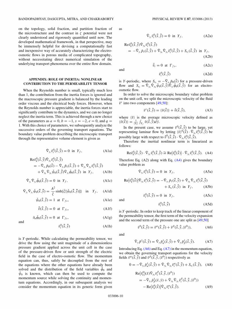
When the Reynolds number is small, typically much lessthan 1, the contribution from the inertia forces is ignored andthe macroscopic pressure gradient is balanced by the leadingorder viscous and the electrical body forces. However, whenthe Reynolds number is appreciable, the inertia forces start tosignificantly contribute to the dynamics, and we can no longerneglect the inertia term. This is achieved through a new choiceof the parameters as a = 0, b = −1, s = −2, e = 0, and q =1. With this choice of parameters, we subsequently analyze thesuccessive orders of the governing transport equations. Theboundary value problem describing the microscopic transportthrough the representative volume element is given as
∇yiv0
i ( �x, �y) = 0 in Yf , (A1a)
Rev0k ( �x, �y)∇yk
v0i ( �x, �y)
= −∇xip0( �x) − ∇yi
p1( �x, �y) + ∇yk∇yk
v0i ( �x, �y)
+∇yk∇yk
ψ0( �x, �y)∇yiφ0( �x, �y) in Yf , (A1b)
∇yi∇yi
φ0( �x, �y) = 0 in Yf , (A1c)
∇yi∇yi
ψ0( �x, �y) = A2
ζsinh{ζ [ψ0( �x, �y)]} in Yf , (A1d)
ψ0( �x, �y) = 1 at �f s, (A1e)
�v( �x, �y) = 0 at �f s, (A1f)
∂nφ0( �x, �y) = 0 at �f s, (A1g)and
v0i ( �x, �y) (A1h)
is Y -periodic. While calculating the permeability tensor, wedrive the flow using the unit magnitude of a dimensionlesspressure gradient applied across the unit cell in the caseof the pressure-driven flow or unit strength of the electricfield in the case of electro-osmotic flow. The momentumequation can, thus, safely be decoupled from the rest ofthe equations where the other equations have already beensolved and the distribution of the field variables φ0 andψ0 is known, which can then be used to compute themomentum source while solving the continuity and momen-tum equations. Accordingly, in our subsequent analysis weconsider the momentum equation in its generic form given
as
∇yiv0
i ( �x, �y) = 0 in Yf , (A2a)
Rev0k ( �x, �y)∇yk
v0i ( �x, �y)
= −∇yip1( �x, �y) + ∇yk
∇ykv0
i ( �x, �y) + Svi( �x, �y) in Yf ,
(A2b)
�vi = 0 at �f s, (A2c)and
v0i ( �x, �y) (A2d)
is Y -periodic, where Svi= −∇xi
p0( �x) for a pressure-drivenflow and Svi
= ∇yk∇yk
ψ0( �x, �y)∇yiφ0( �x, �y) for an electro-
osmotic flow.In order to solve the microscopic boundary value problem
on the unit cell, we split the microscopic velocity of the fluidvε into two components [49,50]:
vε( �x, �y) = 〈v( �x)〉 + ˜v( �x, �y), (A3)
where 〈v〉 is the average microscopic velocity defined as〈v( �x)〉 = 1
|Yf |∫Yf
v( �x, �y)dy.
In the present case, we assume v0( �x, �y) to be large, yetrepresenting laminar flow by letting 〈v〉0( �x) · ∇yk
v0i ( �x, �y) be
possibly large with respect to ˜v0( �x, �y) · ∇ykv0
i ( �x, �y).Therefore the inertial nonlinear term is linearized as
follows:
Rev0k ( �x, �y) · ∇yk
v0i ( �x, �y) ∼= Re
⟨v0
k ( �x)⟩ · ∇yk
v0i ( �x, �y). (A4)
Therefore Eq. (A2) along with Eq. (A4) gives the boundaryvalue problem as
∇yiv0
i ( �x, �y) = 0 in Yf , (A5a)
Re⟨v0
k ( �x)⟩∇yk
v0i ( �x, �y) = −∇yi
p1( �x, �y) + ∇yk∇yk
v0i ( �x, �y)
+ Svi( �x, �y) in Yf , (A5b)
v0i ( �x, �y) = 0 in Yf , (A5c)
andv0
i ( �x, �y) (A5d)
is Y -periodic. In order to keep track of the linear component ofthe permeability tensor, the first term of the velocity expansionand the second term of the pressure one are split as [49,50]
Introducing Eq. (A6) and Eq. (A7) in the momentum equation,we obtain the governing transport equations for the velocityfields vα( �x, �y) and vβ( �x, �y,〈v0〉) respectively as
0 = −∇yip1
α( �x, �y) + ∇yk∇yk
vαi ( �x, �y) + Svi
( �x, �y), (A8)
Re⟨v0
k
⟩(x)∇yk
vβ
i ( �x, �y,〈v0〉)= −∇yi
p1β(x,y) + ∇yk
∇ykv
β
i ( �x, �y,〈v0〉)− Re
⟨v0
k ( �x)⟩∇yk
vαi ( �x, �y). (A9)
033006-10
ELECTRO-OSMOTIC FLOWS THROUGH TOPOGRAPHICALLY . . . PHYSICAL REVIEW E 87, 033006 (2013)
The solution of Eq. (A8) is of the form
vαi ( �x, �y) = kij ( �y)Qj ( �x), (A10)
where Qj = −∇xip0 for pressure-driven flow and Qj = Ej
for electro-osmotic flow.Therefore Eq. (A6) must satisfy
Re⟨v0
k ( �x)⟩∇yk
vβ
i ( �x, �y,〈v0〉)= −∇yi
p1β( �x, �y) + ∇yk
∇ykv
β
i ( �x, �y,〈v0〉)− Re
⟨v0
k
⟩( �x)Qj ( �x)∇yk
kij ( �y). (A11)
Per analogy to solution (A10), there exists a solution for themicroscopic periodic field vβ( �x, �y,〈v0〉) which satisfies
vβ
i ( �x, �y,〈v0〉) = hij ( �y,〈v0〉)Qj ( �x). (A12)
Integrating the ε0 term of the incompressible continuityequation over the period, we get
1
|�|∫
�
∇y �v1 dV + 1
|�|∫
�
∇x �v0 dV
= 1
|�|∫
�
∇y �v1 dV + 1
|�|∫
�
∇x(�vα + �vβ) dV = 0.
(A13)
Due to periodicity and the boundary conditions, we get∫�
∇y �v1 dV =∫
∂�
�v1 · n dS = 0. (A14)
Therefore, Eq. (A13) becomes
1
|�|∫
�
∇x(�vα + �vβ) dV = ∇x · 1
|�|[∫
�
�vαdV +∫
�
�vβ dV
]
= ∇x[〈�vα〉� + 〈�vβ〉�] = 0, (A15)
where 〈·〉� = 1|�|
∫�
· dV .From Eqs. (A7), (A9), and (A12), we get the first order
macroscopic behavior as
〈v0〉� = − ↔K∇xp
0, (A16)
where↔K = 〈↔
k〉� + 〈↔h〉�(〈�v0〉) is the up-scaled permeability
tensor where the second term is the correction arising dueto the incorporation of the nonlinear contribution due to thepresence of the inertial effects. The up-scaled permeabilitytensor is a function of the morphology, liquid fraction, andmean macroscopic velocity in the computational cell, whichin turn is a function of the flow Reynolds number and vanishesfor low Reynolds number flows.
[1] M. Eikerling, A. A. Kornyshev, A. M. Kuznetsov, J. Ulstrup,and S. Walbran, J. Phys. Chem. B 105, 3646 (2001).
[2] F. H. J. van der Heyden, D. J. Bonthuis, D. Stein, C. Meyer, andC. Dekker, Nano Lett. 7, 1022 (2007).
[3] Y. Ren and D. Stein, Nanotechnology 19, 195707 (2008).[4] N. S. K. Gunda, H. Choi, A. Berson, B. Kenney, K. Karan, J. G.
Pharaoh, and S. K. Mitra, J. Power Sources 196, 3592 (2011).[5] A. W. Martinez, S. T. Phillips, and G. M. Whitesides, Anal.
Chem. 82, 3 (2010).[6] P. Mandal, R. Dey, and S. Chakraborty, Lab on a Chip 12, 4026
(2012).[7] N. S. K. Gunda, B. Bera, N. K. Karadimitriou, S. K. Mitra, and
S. M. Hassanizadeh, Lab on a Chip 11, 3785 (2011).[8] L. G. Leal, Advanced Transport Phenomena: Fluid Mechanics
and Convective Transport Processes (Cambridge UniversityPress, New York, 1989).
[9] S. Ghosal, Annu. Rev. Fluid Mech. 38, 309 (2006).[10] R. F. Probstein, Physicochemical Hydrodynamics: An Introduc-
tion (John Wiley and Sons, New York, 1994), p. 400.[11] A. S. Rathore and C. Horvath, J. Chromatogr. A 781, 185 (1997).[12] H. Ohshima, J. Colloid Interface Sci. 210, 397 (1999).[13] S. Levine and G. H. Neale, J. Colloid Interface Sci. 47, 520
(1974).[14] S. Levine, J. R. Marriott, G. H. Neale, and N. Epstein, J. Colloid
Interface Sci. 52, 136 (1975).[15] F. C. Leinweber and U. Tallarek, J. Phys. Chem. B 109, 21481
(2005).[16] D. Coelho, M. Shapiro, and J. Thovert, J. Colloid Interface Sci.
190, 169 (1996).[17] S. Das, S. Chakraborty, and S. K. Mitra, Phys. Rev. E 85, 051508
(2012).
[18] A. Bandopadhyay and S. Chakraborty, Langmuir 28, 17552(2012).
[19] S. Chakraborty and S. Das, Phys. Rev. E 77, 037303 (2008).[20] S. Das, R. Misra, T. Thundat, S. Chakraborty, and S. Mitra,
Energy Fuels 26, 5851 (2012)[21] A. Bandopadhyay and S. Chakraborty, Phys. Rev. E 85, 056302
(2012)[22] S. Chakraborty, J. Phys. D 39, 5356 (2006)[23] J. H. Masliyah and S. Bhattacharjee, Electrokinetic and Colloid
Transport Phenomena (John Wiley & Sons, Hoboken, NJ, 2006).[24] A. A. Saha, S. K. Mitra, and X. Li, J. Power Sources 164, 154
(2007).[25] A. S. Rawool and S. K. Mitra, Microfluidics Nanofluidics 2, 261
(2006).[26] A. Ogawa, J. Rheol. 41, 769 (1997).[27] C. F. Fryling, J. Colloid Sci. 18, 713 (1963).[28] D. E. Elrick, D. E. Smiles, N. Baumgartner, and P. H. Groenevelt,
Soil Sci. Soc. Am. J. 40, 490 (1976).[29] R. Hunter, Zeta Potential in Colloid Science: Principles and
Applications (Academic Press, London, 1981).[30] A. Dasgupta and R. K. Agarwal, J. Compos. Mater. 26, 2736
(1992).[31] A. J. Majda and P. E. Souganidis, Nonlinearity 7, 1
(1994).[32] G. Laschet, S. Rex, D. Bohn, and N. Moritz, Numer. Heat
Transfer, Part A 42, 91 (2002).[33] G. Laschet, Comput. Methods Appl. Mech. Eng. 191, 4535
(2002).[34] W. Zijl and A. Trykozko, Comput. Geosci. 6, 49 (2002).[35] D. DasGupta, S. Basu, and S. Chakraborty, Phys. Lett. A 348,