HAL Id: hal-02868061https://hal.archives-ouvertes.fr/hal-02868061

Submitted on 9 Nov 2020

HAL is a multi-disciplinary open accessarchive for the deposit and dissemination of sci-entific research documents, whether they are pub-lished or not. The documents may come fromteaching and research institutions in France orabroad, or from public or private research centers.

L’archive ouverte pluridisciplinaire HAL, estdestinée au dépôt et à la diffusion de documentsscientifiques de niveau recherche, publiés ou non,émanant des établissements d’enseignement et derecherche français ou étrangers, des laboratoirespublics ou privés.

Electrochemical studies of steel rebar corrosion in clay:Application to a raw earth concrete

Joanna Eid, Hisasi Takenouti, Bachir Ait Saadi, Said Taibi

To cite this version:Joanna Eid, Hisasi Takenouti, Bachir Ait Saadi, Said Taibi. Electrochemical studies of steel rebar cor-rosion in clay: Application to a raw earth concrete. Corrosion Science, Elsevier, 2020, 168, pp.108556.10.1016/j.corsci.2020.108556. hal-02868061

1

Electrochemical study of steel rebar corrosion in clay:

Application to a raw earth concrete.

Joanna Eid1,2*, Hisasi Takenouti3, Bachir Ait Saadi4, Said Taibi1

1 Laboratoire Ondes et Milieux Complexes, UMR 6294, CNRS - Normandie Université, Université Le Havre Normandie, 53 rue Prony, 76600 Le Havre, France, said.taibi@univ-lehavre.fr

2 Civil Engineering Department, Holy Spirit University of Kaslik (USEK), Jounieh, Lebanon, joannaeid@usek.edu.lb

3 Laboratoire Interfaces et Systèmes Electrochimiques, UMR 8235, CNRS - Sorbonne Université, 4 place Jussieu, 75252 Paris CEDEX 05, France, hisasi.takenouti@upmc.fr

4 Laboratoire de microscopie électronique et des sciences des matériaux, Université Sciences & Technologie d’Oran, BP 1505, El Ménaouer, Oran, Algeria, bac.aitsaadi@gmail.com

* Corresponding author. E-mail: joannaeid@hotmail.com; Phone: +33 6 4862 9147; +961 9 600 931

___________________________________________________________________________

Abstract

Reinforcement feasibility of a new ecological earth concrete was examined. Steel rebar

corrosion, when in contact with three different types of clayey soil, was investigated using

electrochemical methods, potentiodynamic voltammetry and impedance spectroscopy (EIS).

Results have shown that the voltammetry method overestimates the corrosion rate while EIS

supplies the most reliable results. Corrosion rate decreased and a steady state was reached

after four months of contact. The type of clay does not have a significant influence on the

corrosion rate of the steel rebar, and the average value of 3 was considered

acceptable for the lifetime of the structure.

Keywords: raw earth concrete, eco-materials, clay-steel interaction, electrochemical analyses,

polarization resistance, EIS.

2

1. Introduction

Nowadays, ecological issues are important in the field of construction and civil engineering.

Standard concrete requires, for its production, huge grey energy consumption. In addition, it

needs natural aggregates, as sand and gravel, having significant impacts on the nature [1], like

the destruction of beaches and mountains [2].

In order to reduce the environmental impact of standard concrete, the use of energy-efficient

materials is necessary [3]. Therefore, many researchers tend to study the behaviour of eco-

geo-materials, as new construction resources, such as dredged sediment, recycled aggregates,

or raw earth [4] [5]. One of the alternatives is using natural soils (raw earth) as a basic

material.

A new earth concrete was developed and patented in Normandy, France [6] [7] [8]. It is

composed of 87 % of raw earth treated with 9% of cement and/or 3% of lime. It can also be

strengthened with recycled concrete aggregates RCA [9] to improve its mechanical properties

while remaining ecological. This earth concrete presents a satisfactory mechanical behaviour

when structural elements are acting in compression, e.g. bearing walls. However, as in the

case of standard concrete, when structural elements are working in bending or tension, e.g.

beams, the concrete presents a low tensile strength which requires the use of steel

reinforcements. Likewise, this low tensile strength affects the shrinkage behaviour of the earth

concrete [10]. Using ecological reinforcements such as bamboo, liana, or vegetable fibres can

be possible in the future with advanced studies [11] [12]. Thus, with the new earth concrete,

steel reinforcement is still necessary to construct buildings, with structural elements acting in

tension.

In the standard concrete, the environment is alkaline (pH value as high as 12.5). This

environment promotes the formation of a protective film on the steel surface, which reduces

3

the corrosion rate [13]. However, due to the porosity of concrete, carbonation [14] and ingress

of chloride ions [15] may occur, which will decrease the pH value and stimulate the corrosion

process. In earth concrete, the environment is also alkaline, when it is treated with binders

(cement and lime), but it is also composed of natural clayey soil that is not inert, like the case

of sand and gravel present in standard concrete. So, to study the corrosion of steel in earth

concrete, the interaction between the natural clayey soil and the steel should be considered.

Natural soil is a highly non-homogeneous environment, composed of different minerals and

chemical compounds. Many soil parameters influence the corrosion of the steel [16] which

are the particle size [17] [18], pH [19], moisture content [20] [21], concentration of dissolved

oxygen [21] [22], nature of salt ions, and organic content [23]. According to the soil’s particle

size distribution, its resistivity varies and affects significantly the corrosion of the steel in soil

[23]. Among minerals, clays are the most reactive with their environment with the presence of

water; they increase soil’s conductivity [16]. So, understanding their interaction with the steel

is highly important, especially when the soil is used to construct buildings.

Studies reported in the literature discuss mostly bentonite-iron interaction. El-Shamy et al.

[20] showed that the corrosion rate of pipelines in contact with bentonite is proportionally

related to water content, as large as the moisture content is below 40%. Kaufhold et al. [24]

showed that Na-bentonites are slightly less corrosive than Ca-bentonites, and that highly

charged smectites are less corrosive than low charged ones. They also found out a formation

of a 1:1 Fe-silicate mineral. Earlier, Ishidera et al. [25], also found out that the smectite clay

was destabilized to form a 1:1 phyllosilicate. Schlegel et al. [26] showed a transformation in

clay layers and a decrease in the corrosion rate with time. In iron-rich clay, Yan et al. [27]

showed that the presence of Fe oxides in clay increases the reaction rate for both anodic and

cathodic processes of pipeline steel.

4

Different techniques are proposed to evaluate the corrosion process and to measure the

corrosion rate. Among all, electrochemical techniques are the most used. In different studies,

the electrochemical impedance spectra showed two relaxation time constants with capacitive

behaviour [16] [27].

The literature review shows that many studies dealt with the interaction between soil and

carbon steel in the fields of archaeology [28] [29], pipelines [30], and radioactive waste

management [24] [31]. These environments (high temperature, anaerobic, compacted soil,

etc…) are very different from those of construction. In this field, only a few studies were

devoted to earth walls and backfill reinforcement [32]. As far as we know, no study dealt with

the corrosion of steel rebars in contact with earth concrete.

The aim of this paper is to investigate the corrosion rate of steel rebars embedded in raw

earth. Results will validate the feasibility of reinforced earth concrete.

2. Methods

When a steel rebar is in contact with soil, the corrosion process takes place [33] [34] [35]. In

this study, the interaction between a carbon steel rebar and three types of clayey soil,

kaolinite, montmorillonite and natural silt, was investigated using two electrochemical

methods to estimate the corrosion rate [36] [37].

2.1. Principles of electrochemical methods

A classical three electrodes cell constituted of a working (WE), a reference (RE) and a

counter electrode (CE) was used. Electrodes were in contact with the clay which is a corrosive

environment that constitutes the electrolyte. These electrodes were connected to a potentiostat

which is both a control and a measuring device. It maintains the potential of the WE constant

with respect to the RE by adjusting the current at the CE.

5

Generally, to study an electrochemical corrosion system, three main measurements can be

done, open circuit potential (OCP, or ), potentiodynamic polarizations (also called

potentiodynamic voltammetry) that estimate the corrosion current density ( ) and Tafel

constants for anodic and cathodic processes, and electrochemical impedance spectroscopy

(EIS). Generally, experimental spectra were then reproduced by an adequate equivalent

circuit. From these measurements, the corrosion rate of the WE in contact with electrolyte can

be evaluated.

2.2. Experimental setup

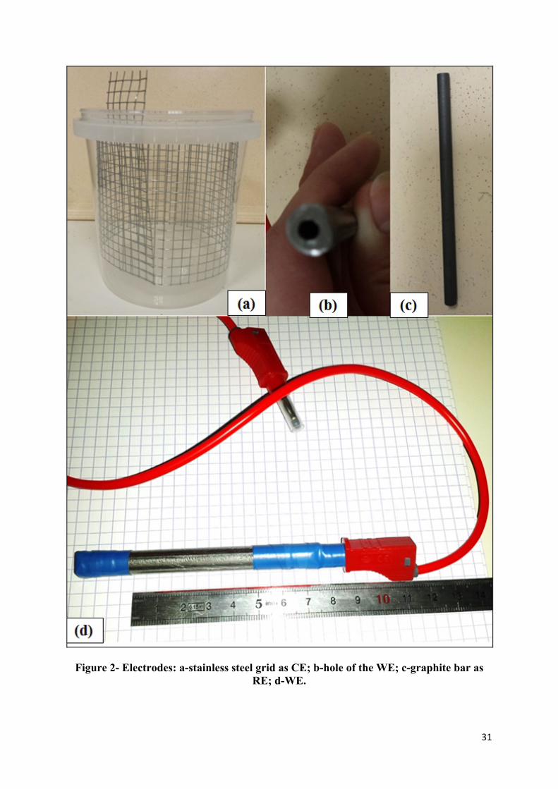
Figure 1 presents a descriptive scheme of the experimental setup used in this study. The

counter electrode was a stainless-steel grid (Figure 2). The steel rebar, generally used in

reinforced concrete, constituted the working electrode (Figure 2) with a drilled hole at one end

(Figure 2-b) to ensure electrical connection to the potentiostat. This steel rebar had a smooth

surface with a diameter of 10 mm. It was coated with an insulating tape at both ends to limit

the contact area with the soil to 5 cm (length). The contact area of the WE for all experiments

was then 15.7 cm2. The reference electrode was a graphite rod (Figure 2) throughout the

experimental process. Table 1 shows the potential of the graphite rod embedded in clay with

respect to SCE. The potential shows an exponential decay with time. All potentials were

related to SCE scale.

First, the CE was placed in the slightly conical mould wall. A small portion of the CE extends

above the top surface of the mould, in order to be connected to the potentiostat (Figure 2).

Second, the wetted soil, with a water content slightly above the liquid limit , was poured

and vibrated. Third, the WE was inserted in the centre of the poured soil. Finally, the RE was

inserted between the WE and the CE. The mould was then covered with a pre-cut lid. All

6

apertures were sealed carefully with silicone mastic to avoid evaporation and to maintain the

soil water content throughout the experiment.

The potentiostat used in this study was Gamry® Interface 1000. Once the system was

stabilized (i.e. constant OCP), the following procedure was realized:

1. OCP was measured during the first 5 minutes to ascertain the free potential value.

2. EIS was then measured at OCP with a frequency ranging between 100 kHz and 10

mHz or less, by 5 or 10 points per decade. The amplitude of AC signal was 10

3. After the collection of impedance spectrum, the electrode was kept at the open circuit

for one hour, followed by 5 minutes of OCP measurement.

4. Potentiodynamic polarization curve was then collected. The potential was scanned

from -50 to +50 mV with respect to OCP at a scan rate of 1 .

This set of measurements was repeated continuously for 2 days, then once a day for a week,

then once a week for one month, then once a month for 3 months and finally every 3 months.

Altogether, the experiments were continued for six months.

2.3. Calculation and analyses

From these measurements, two sets of results were obtained, the current I in function of the

potential (voltammogram) and the impedance (complex number) in function of the AC

perturbing signal. The objective was to evaluate the corrosion current density ( ) then

to calculate the corrosion rate ( ).

From the potentiodynamic voltammetry, was deduced from the first Stern-Geary equation

[38] (equation 1) with the faradaic current passing through the WE interface.

7

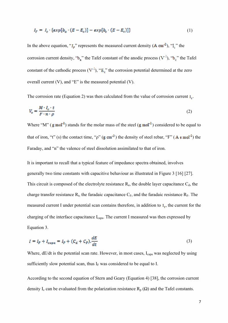
(1)

In the above equation, “ ” represents the measured current density ( ), “ ” the

corrosion current density, “ ” the Tafel constant of the anodic process ( ), “ ” the Tafel

constant of the cathodic process ( ), “ ” the corrosion potential determined at the zero

overall current (V), and “E” is the measured potential (V).

The corrosion rate (Equation 2) was then calculated from the value of corrosion current .

(2)

Where “M” ( ) stands for the molar mass of the steel ( ) considered to be equal to

that of iron, “t” (s) the contact time, “ρ” ( ) the density of steel rebar, “F” ( ) the

Faraday, and “n” the valence of steel dissolution assimilated to that of iron.

It is important to recall that a typical feature of impedance spectra obtained, involves

generally two time constants with capacitive behaviour as illustrated in Figure 3 [16] [27].

This circuit is composed of the electrolyte resistance Re, the double layer capacitance Cd, the

charge transfer resistance Rt, the faradaic capacitance CF, and the faradaic resistance RF. The

measured current I under potential scan contains therefore, in addition to , the current for the

charging of the interface capacitance Icapa. The current I measured was then expressed by

Equation 3.

(3)

Where, dE/dt is the potential scan rate. However, in most cases, Icapa was neglected by using

sufficiently slow potential scan, thus IF was considered to be equal to I.

According to the second equation of Stern and Geary (Equation 4) [38], the corrosion current

density Ic can be evaluated from the polarization resistance Rp (Ω) and the Tafel constants.

8

(4)

The polarization resistance can be calculated either from the slope of the current-potential

curve at the corrosion potential Ec, as well from the impedance results by fitting the

impedance spectra with the equivalent electrical circuit or the extrapolation of Nyquist plot to

the low frequency limit (Equation 5). Note that does not contain the term of the electrolyte

resistance .

(5)

3. Materials

Three types of soil were analysed in this study: natural silt, kaolinite clay and montmorillonite

clay. Their X-ray diffractogram is presented in Figure 4 in order to identify their mineralogy.

The soils were initially moistened to become a mud by adding an appropriate amount of water

to the dry natural material.

Table 2 presents the water content of the slurry, w , the pH,

and the electrical conductivity of the considered soils. The water used was doubly deionised

water.

3.1. Natural silt

The natural soil used in this study was silt retrieved from earthmoving works. It constituted

the principal component of the earth concrete (cf. Table 3). Based on these properties and its

grading curves, the soil used was classified as sandy loam SL(SM) by the USCS classification

9

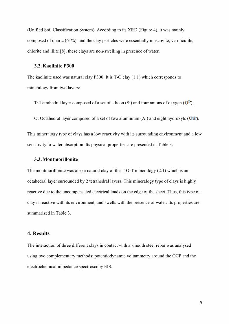
(Unified Soil Classification System). According to its XRD (Figure 4), it was mainly

composed of quartz (61%), and the clay particles were essentially muscovite, vermiculite,

chlorite and illite [8]; these clays are non-swelling in presence of water.

3.2. Kaolinite P300

The kaolinite used was natural clay P300. It is T-O clay (1:1) which corresponds to

mineralogy from two layers:

T: Tetrahedral layer composed of a set of silicon (Si) and four anions of oxygen ( );

O: Octahedral layer composed of a set of two aluminium (Al) and eight hydroxyls ( ).

This mineralogy type of clays has a low reactivity with its surrounding environment and a low

sensitivity to water absorption. Its physical properties are presented in Table 3.

3.3. Montmorillonite

The montmorillonite was also a natural clay of the T-O-T mineralogy (2:1) which is an

octahedral layer surrounded by 2 tetrahedral layers. This mineralogy type of clays is highly

reactive due to the uncompensated electrical loads on the edge of the sheet. Thus, this type of

clay is reactive with its environment, and swells with the presence of water. Its properties are

summarized in Table 3.

4. Results

The interaction of three different clays in contact with a smooth steel rebar was analysed

using two complementary methods: potentiodynamic voltammetry around the OCP and the

electrochemical impedance spectroscopy EIS.

10

4.1. Potentiodynamic voltammetry results

Figure 5 displays the time evolution of log(I)-E curves for steel-Montmorillonite couple. One

over two experimental data were plotted by symbols. Lines corresponds to fitted curves

according to Equation 2 by non-linear simplex regression calculation. The consistency

between these two data was satisfactory since the coefficient of determination , the

correction factor, was greater than 0.999 for all cases.

Excluding the very early stage, it can be noticed that the cathodic current density increased

with contact time of the steel in the soil whereas the anodic reaction rate decreased. The

potential shifted towards a more anodic direction while the corrosion current density

decreased. Following, the variation of various voltammetry parameters for the three soils was

presented.

4.1.1. OCP and Ec variation

Figure 6 presents the variation of the measured (OCP) and that was calculated by non-

linear fitting of I-E curves (Equation 2). The curves were slightly consistent. Both potentials

varied similarly. In the case of silt, it increased in the first three days, while in the case of

kaolinite, it increased in the first ten days. Both then decreased. In contrast, for

montmorillonite, they decreased monotonically in the first 2 days and then increased after.

4.1.2. Variation of corrosion current density

Figure 7 shows the variation of the corrosion current density determined by

potentiodynamic voltammetry, Equation 2. Like the potential variation, of silt and kaolinite

presented a similar feature. The initial was low, 0.7 and 1.3 , respectively for silt

and kaolinite. It decreased slightly on the first day of contact time; then it remained almost

constant for about a week, then increased steeply after. This steep current increase was

11

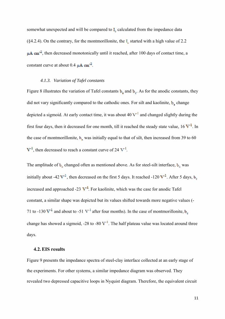
somewhat unexpected and will be compared to calculated from the impedance data

(§4.2.4). On the contrary, for the montmorillonite, the started with a high value of 2.2

, then decreased monotonically until it reached, after 100 days of contact time, a

constant curve at about 0.4 .

4.1.3. Variation of Tafel constants

Figure 8 illustrates the variation of Tafel constants and . As for the anodic constants, they

did not vary significantly compared to the cathodic ones. For silt and kaolinite, change

depicted a sigmoid. At early contact time, it was about 40 and changed slightly during the

first four days, then it decreased for one month, till it reached the steady state value, 16 . In

the case of montmorillonite, was initially equal to that of silt, then increased from 39 to 60

, then decreased to reach a constant curve of 24 .

The amplitude of changed often as mentioned above. As for steel-silt interface, was

initially about -42 , then decreased on the first 5 days. It reached -120 . After 5 days,

increased and approached -23 . For kaolinite, which was the case for anodic Tafel

constant, a similar shape was depicted but its values shifted towards more negative values (-

71 to -130 and about to -51 after four months). In the case of montmorillonite,

change has showed a sigmoid, -28 to -80 . The half plateau value was located around three

days.

4.2. EIS results

Figure 9 presents the impedance spectra of steel-clay interface collected at an early stage of

the experiments. For other systems, a similar impedance diagram was observed. They

revealed two depressed capacitive loops in Nyquist diagram. Therefore, the equivalent circuit

12

will be composed of the electrolyte resistance , two resistances (charge transfer resistance

and faradaic resistance ), and their corresponding capacitances. This circuit was very

close to Figure 3, where the capacitive behaviour was presented by pure capacitance; whereas

in Figure 10-a, reckon depressed feature of capacitive loops, CPE was used. The CPECd

represented the contribution of the electrochemical double layer capacitance. The couple

RF//CPEF was allocated to the redox process taking place with corrosion products and

accumulated on the steel surface. The electrochemical reaction involving a redox process is

presented in §5.2. On the contrary, for montmorillonite, after about 20 days of contact with

the steel rebar, an additional capacitive loop started to appear in the Nyquist diagram at the

high frequency side and increased after about 2 months. The equivalent circuit presented in

Figure 10 was used for parameter fitting calculations.

The circuit elements in Figure 10 are the following:

: Electrolyte resistance between RE and WE ( )

: Charge transfer resistance ( )

: CPE element for double layer capacitance ( )

: Power coefficient of CPE (dimensionless)

: Faradaic resistance associated with redox process ( )

: CPE element for faradaic capacitance ( )

: Power coefficient of CPE for the redox process (dimensionless)

: Resistance representing ionic conduction through the surface layer ( )

: CPE element for surface layer ( )

: Power coefficient of surface layer (dimensionless)

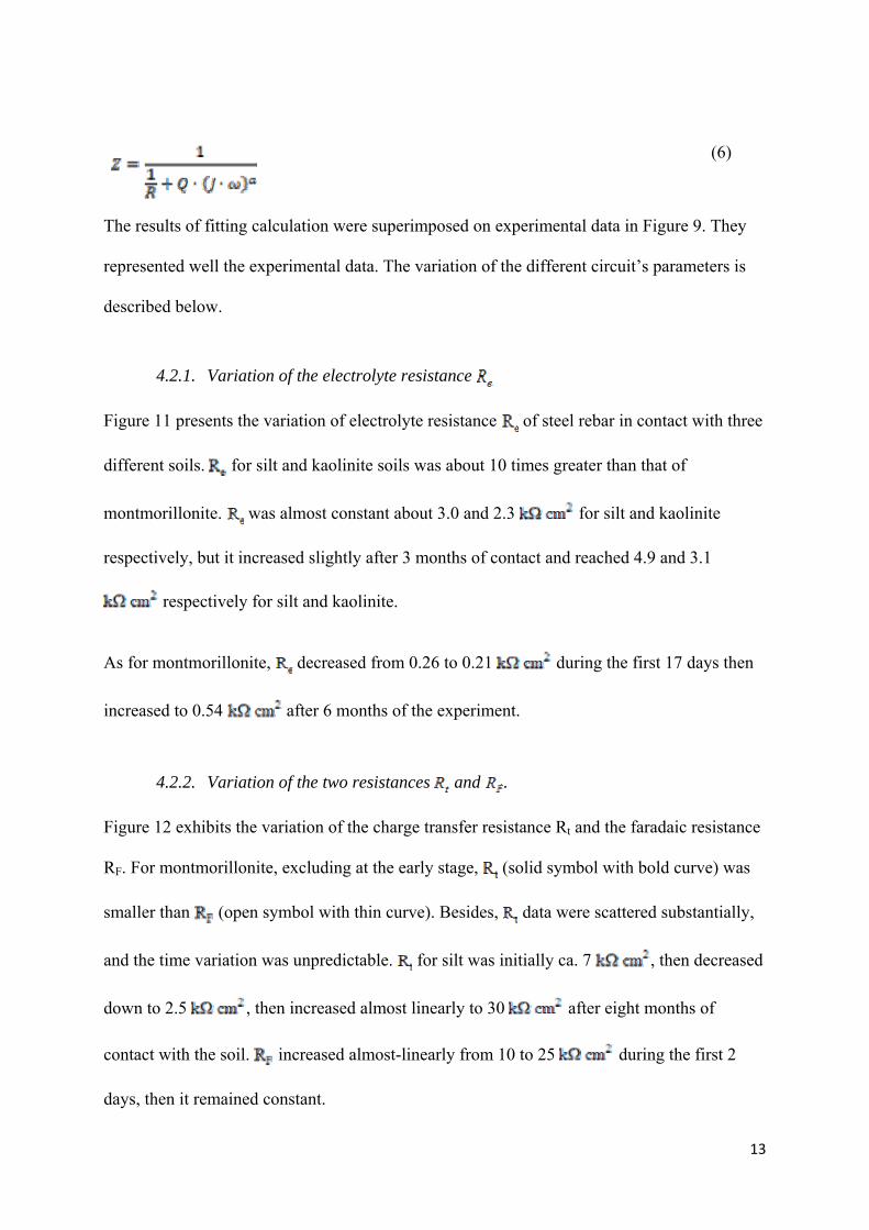
The impedance of a CPE element (Q, a) in parallel with a resistance R is:

13

(6)

The results of fitting calculation were superimposed on experimental data in Figure 9. They

represented well the experimental data. The variation of the different circuit’s parameters is

described below.

4.2.1. Variation of the electrolyte resistance

Figure 11 presents the variation of electrolyte resistance of steel rebar in contact with three

different soils. for silt and kaolinite soils was about 10 times greater than that of

montmorillonite. was almost constant about 3.0 and 2.3 for silt and kaolinite

respectively, but it increased slightly after 3 months of contact and reached 4.9 and 3.1

respectively for silt and kaolinite.

As for montmorillonite, decreased from 0.26 to 0.21 during the first 17 days then

increased to 0.54 after 6 months of the experiment.

4.2.2. Variation of the two resistances and .

Figure 12 exhibits the variation of the charge transfer resistance Rt and the faradaic resistance

RF. For montmorillonite, excluding at the early stage, (solid symbol with bold curve) was

smaller than (open symbol with thin curve). Besides, data were scattered substantially,

and the time variation was unpredictable. for silt was initially ca. 7 , then decreased

down to 2.5 , then increased almost linearly to 30 after eight months of

contact with the soil. increased almost-linearly from 10 to 25 during the first 2

days, then it remained constant.

14

for kaolinite showed a bell-shaped curve. The initial and final values were both 2.8

and the resistance was maximal at 3 days with 11 . increased similarly for silt, but

slightly steeper, almost-linearly from 6 to 40 for 30 days to reach a steady state.

for montmorillonite was almost constant around 3 , on the first day, then decreased to

1 at about four days. Over one week, it increased almost linearly. Its was smaller

than in contrast to other cases. It depicted sigmoid, from 2 to 25 .

4.2.3. Variation of the effective capacities and

The quantitative comparison of CPE was not an easy task since this variable was defined in

both CPE element Q and power coefficient a. For that reason, the effective capacitance of

each CPE element was calculated using the equation proposed by Brug et al. [39]. For a

circuit , i.e. composed of electrolyte resistance in series with a parallel

linking of CPE element and the charge transfer resistance , the effective capacitance C can

be expressed by equation 7:

(7)

Figure 13 presents the variation of the effective double layer capacitance and the faradic

capacitance .

(solid symbols with bold curve) for both silt and kaolinite increased with contact time.

For silt, it changed from 50 during one hour of contact time to 10 after 9

months. For kaolinite, it ranged between 60 and 16 for the same period.

Between one and two weeks, the capacitance increase was slower and was about 700 .

15

For montmorillonite, its variation was different. It increased from 80 to 700 during

the first month and then decreased significantly.

of silt was small at the beginning, 35 and reached a value as high as 25

after 6 months of contact time. for kaolinite remained constant during the first day, then it

increased progressively. After 8 months, it was about 6 . The variation of this

capacitance for montmorillonite was complex; it increased slightly during the first day, then it

decreased from 400 to 70 for 2 days, then it increased after. The value at 8 months

was the smallest among the three soils examined.

4.2.4. Variation of the corrosion current density

Using Equation 3, the corrosion current density was evaluated from EIS data. So, called

Stern-Geary constant B was determined by parameters fitting of voltammogram, Figure 8.

Figure 14 displays the variation of the corrosion current density calculated with as

mentioned above (Equation 6). This relationship was introduced to an electrochemical system

with anodic and cathodic Tafel relationship. However, the same equation was valid when a

redox process was involved in the corrosion mechanism [40]. Figure 7 shows the same

relationship when was determined from polarization curves. The initial values were

similar for these two methods. However, a marked divergence can be noticed for a long

contact time. determined by EIS decreased continuously up to three months, then

increased very slightly for silt and kaolinite; whereas for montmorillonite, decreased during

the whole period examined in this study.

Figure 7 includes also the corrosion rate expressed by thickness loss. After 8 months, the

corrosion rate was smaller than 3 for all clayey soils examined.

16

5. Discussion

5.1. Identification of corrosion products

The corrosion products formed at the surface of steel rebar were studied by XPS and XRD.

XPS analysis was carried out between 0 and 1350 eV after etching during 720 s of the

electrode surface. Figure 15 presents, as for an example, the XPS spectrum of corrosion

products in contact with montmorillonite, after two years exposure, around the peak

corresponding to Fe2p. The results of deconvolution of this peak were indicated in the figure.

The Fe2+ peak corresponds to Fe2O3. The peak Fe3+ corresponded to the magnetite formed by

a transformation of Fe(OH)2. The multiple peaks indicated the presence of magnetite. A small

amount of siderite, FeCO3 was also detected.

The XRD also detected, not illustrated here, the magnetite and the peaks of montmorillonite,

quartz and goethite (α-FeOOH). For the other two corrosive environments, XPS spectra were

similar and identified the same substances with slightly different proportion for peak area.

XRD pattern showed the presence of magnetite.

The main corrosion product was therefore magnetite. According to E-pH diagram, in neutral

medium, which is our case at the beginning of experiments (cf. Table 2), OCP for the three

media examined (located between -0.54 and -0.75 V vs. SCE ) indicated that was

thermodynamically stable species [41]. The examined corrosion products formed on the steel

rebar embedded in clayey soils were mainly magnetite with a small amount of siderite.

According to Nakono, with geochemistry database [42], will be formed in this

potential - pH domain.

17

5.2. Corrosion process

In most cases, the impedance spectra showed two capacitive loops. These two capacitive loop

diagrams can be explained by the following corrosion mechanism:

For the anodic process:

[1]

[2]

[3]

[4]

[5]

Reaction of Step [1] is the formation of monovalent adsorbed species. This intermediate

reaction species leads to the active dissolution through reaction [2] and the formation of

passive species by reaction [3]. The latter is oxidized into (reaction [4]).

These species dissolve further in ferric species by reaction [5]. Step [4] is reversible giving

rise to the faradaic capacitance CF. Two intermediate reactions, and at

the surface, may induce two relaxation time constants. However, no such time constants were

observed. This phenomenon can be explained by the fact that these time constants were too

short to be observed experimentally.

The cathodic process will be the reduction of dissolved oxygen:

[6]

All these reactions were electrochemical with charge transfer. Step [4] was reversible, which

induced a capacitive behaviour in electrochemical impedance. Corrosion process was

governed by the equality of the electron formation (Steps 1 to 5) and their consumption (Step

18

6). Results suggested that a large amount of will be formed because value was high

(cf. Figure 13).

To facilitate the discussion, the surface film formed will be called magnetite even if siderite

was also detected.

In the three soils media, the cathodic Tafel constant was never close to zero (cf. Figure 8)

excluding that of the reaction kinetics (Step 6) because it was never entirely controlled by the

diffusion, in spite of the electrode embedded in a pasty soil. The diffusion limiting current

density of dissolved oxygen should be lower in the presence of clays than that for an electrode

directly immersed in a solution; the voltammetry curves did not show that the cathodic

process was controlled by convective diffusion. Thus, Step 6 was mostly governed by the

activation process.

On the other hand, the anodic branch did not show that IF was independent of the potential;

whereas the dissolution of passive species may be chemical. According to Seo and Sato [43],

the anion-doped hydro-oxide may depend on the potential of the electrode.

OCP corresponded to the overall current density equal to 0 ( ). If magnetite

film become more stable with time, the reaction rate of Step 5 may decrease, leading OCP

moving towards a more anodic direction (Figure 5).

5.3. Loop appearance at high frequencies for Montmorillonite

The insert in Figure 16 illustrates the additional high frequency loop observed for this clay

after 6 months of contact time. This loop can be simulated with a CPE//R. The calculated

remained practically constant and it was equal to 200 with respect to contact time. The

resistance associated with the high frequency loop was about 200 . The effective

capacitance was equal to 0.04 . This high frequency loop was likely due to the

19

formation of a compact montmorillonite layer, probably containing corrosion products, on the

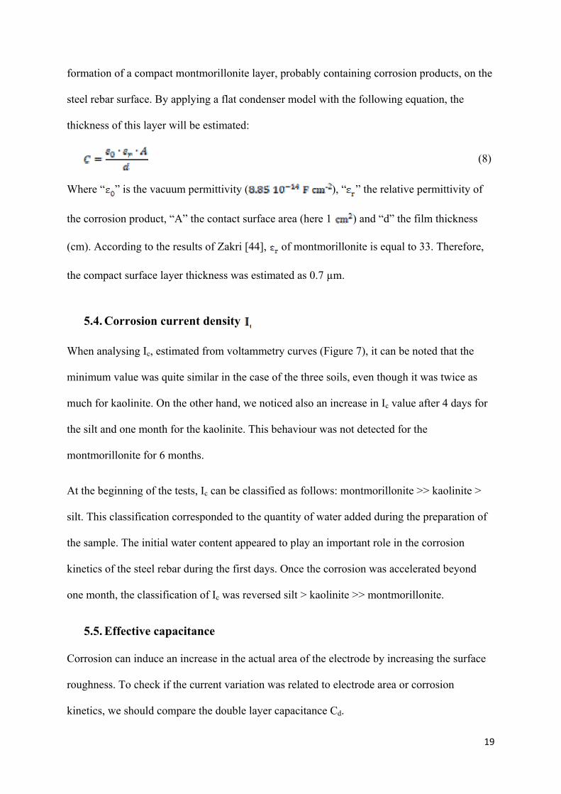
steel rebar surface. By applying a flat condenser model with the following equation, the

thickness of this layer will be estimated:

(8)

Where “ ” is the vacuum permittivity ( ), “ ” the relative permittivity of

the corrosion product, “A” the contact surface area (here 1 ) and “d” the film thickness

(cm). According to the results of Zakri [44], of montmorillonite is equal to 33. Therefore,

the compact surface layer thickness was estimated as 0.7 µm.

5.4. Corrosion current density

When analysing Ic, estimated from voltammetry curves (Figure 7), it can be noted that the

minimum value was quite similar in the case of the three soils, even though it was twice as

much for kaolinite. On the other hand, we noticed also an increase in Ic value after 4 days for

the silt and one month for the kaolinite. This behaviour was not detected for the

montmorillonite for 6 months.

At the beginning of the tests, Ic can be classified as follows: montmorillonite >> kaolinite >

silt. This classification corresponded to the quantity of water added during the preparation of

the sample. The initial water content appeared to play an important role in the corrosion

kinetics of the steel rebar during the first days. Once the corrosion was accelerated beyond

one month, the classification of Ic was reversed silt > kaolinite >> montmorillonite.

5.5. Effective capacitance

Corrosion can induce an increase in the actual area of the electrode by increasing the surface

roughness. To check if the current variation was related to electrode area or corrosion

kinetics, we should compare the double layer capacitance Cd.

20

Figure 13 shows that change was similar in both value and evolution over time, up to 30

hours of steel-soil contact. They increased almost linearly in the semi-logarithmic plane, i.e.

their increase followed an exponential law. Some acceleration of their increase was observed

when Ic increased rapidly (excluding the case of montmorillonite). For the last clay sample,

we observed a formation of a relatively thin protective film. The continuous decrease of as

well as in the latter medium can be explained by the formation of the barrier layer.

The faradaic capacitance CF (open symbols with thin curves) in Figure 13, gave information

on the redox process of Step 4. The greater the amount of magnetite available for the

reversible reaction was, the larger the value was. During one day of contact, remained

stable. The steel-silt system was initially about five times smaller but later it increased to

reach the value like the other two media. Hence, at the beginning, there will be less amount of

the magnetite in this environment that have low water content. Steps 1 and 3 in this

environment would be slower. However, increased after this initial period and continued

to increase thereafter.

For kaolinite, the CF value remained stable for one day, and then it increased. However, Ic

also increased after the first day. Therefore, a strong correlation existed between CF and Ic for

the steel electrode in contact with kaolinite. As for silt, the CF value indicated a continuous

increase in surface accumulation of magnetite and an increase of Ic determined by

voltammetry after 10 hours of contact. variation for the steel-montmorillonite interface

was more complex.

It can be noticed that Cd and CF varied similarly (excluding the case of montmorillonite above

one day of contact time). A particular behaviour of montmorillonite can be explained by the

formation of a compact surface layer. The magnetite is an electronic conducting species,

therefore, the increase of CF, that was the amount of magnetite at the steel surface cause a

21

greater Cd value. In other terms, Cd was not merely related to the surface roughness of the

steel, but also to the expanded surface area of corrosion products accumulated on the steel

surface. At the very beginning of experiments, where the accumulation of magnetite on the

steel surface was negligible, the value of Cd that was frequently observed for the double layer

capacitance, was several tens of µ .

5.6. Charge transfer resistance Rt and Faradaic resistance

Excluding the early stage of the steel corrosion in contact with montmorillonite, t < 3 days,

the lower the corrosion current density determined by the voltammetry was, the greater the

charge transfer resistance was (Figure 12). This was rather an unusual situation. However, CF

(Figure 13) and Rt varied qualitatively in a similar way. The charge transfer resistance also

involved the reaction step [4], and during that period, magnetite formed had lost its reactivity.

The formation of a surface film with montmorillonite may likely be related to this

phenomenon.

It can be seen that RF (Figure 12) was strongly correlated with Ic, the higher RF was, the

higher the corrosion current density was. An exception occurred for a short contact period for

montmorillonite where we found out that Rt < RF. Thus, the corrosion current density was

expected to decrease with contact time. However, we realized that the increase in RF was fast

between one and ten days for montmorillonite. Precisely, in this period, CF decreased. Since

CF was related to the charge stored at the interface, the decrease in the reactivity of the

passive film lead to a lower quantity of this species available for the redox reaction of Step 4.

The corrosion rate depended on both the anodic and cathodic processes. The corrosion

potential was defined by the equality of these two current densities in absolute value.

Variation of OCP, measured just before the start of the voltammetry measurement, is

discussed below.

22

5.7. OCP and Ec

Figure 6 shows that at early contact time, OCP remained almost constant for silt, whereas it

increased for kaolinite and decreased for montmorillonite. After one day of contact, OCP

shifted towards a more anodic direction for all the three interfaces. For silt and kaolinite, OCP

showed a maximum than decreased; whereas for montmorillonite, it continued to increase.

The higher the Ic was, the more anodic OCP was.

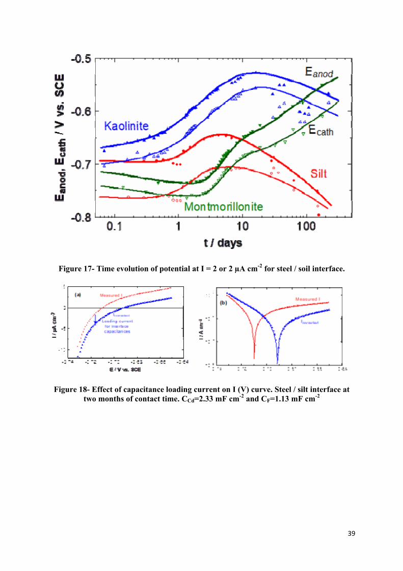
Figure 17 presents the potential variation at anodic or cathodic current equal to ± 2 µA cm-2

for the three systems examined. These potentials varied similarly to OCP, i.e. the decrease of

the corrosion current Ic determined by voltammetry was induced by the slow-down of both

processes. Conversely, the increase of corrosion current density was determined by the

acceleration of both processes.

We realized a difference between OCP and Ec for the three steel-clay interfaces. Ec was

determined by the overall zero current on the voltammetry plots (Figure 6). The gap was

small at the beginning of the experiment and then increased with time. However, the steel-silt

and steel-kaolinite systems showed a larger difference compared with montmorillonite

medium.

The origin of this potential difference between OCP and Ec is discussed in the next section.

5.8. Effect of interface capacitance to

As shown in Equation 3, the current measured during voltammetry experiments contained the

current for charging the interface capacitance whereas the corrosion rate should be determined

by the faradaic current IF. Consequently, the current measured by voltammetry curve

overestimated the corrosion current density. Figure 13 shows that the interface capacitance, C

23

(= Cd + CF) increased from ca. 200 µF cm-2 to more than 10 mF cm-2 for silt and kaolinite

media.

For C = 1 mF cm-2 with the scan rate dE/dt = 1 mV s-1, Icapa = 1 µA cm-2. When C reached this

magnitude, we observed a significant increase of Ic by voltammetry for silt and kaolinite

media. As for montmorillonite, after 10 days, C decreased, and Figure 7 shows the corrosion

current density decreasing with time.

In Figure 18, the voltammograms corrected for the charging current of interface capacitance is

presented for steel-silt at two months contact time. Figure 18-a is relative to the linear I-E

curve. The correction for charging current decreased the current while increasing the

polarization resistance. It increased from 5.06 to 12.9 kΩ cm-2 by subtracting the contribution

of the interface capacitance. Ec, i.e. the zero overall current, shifted towards a more anodic

direction by 21 mV. Ec was determined by the correction of interface capacitance and was

equal to OCP. It was thus demonstrated that the difference of OCP and Ec observed was really

induced by the potential scan, certainly too fast for these corroding systems because of a

marked increase of interface capacitance.

Figure 18-b displays the same results in the Tafel plot. The fitting of these curves with

Equation 2 resulted in an Ic equal to 2.39 and 0.856 µA cm-2.

The corrosion kinetics by impedance measurement required the Stern-Geary coefficient B

[38]. B determined by parameter fitting calculation of the measured current density and that

of the corrected C charging, cf. Figure 18-a, was respectively 12.1 and 11.0 mV. The former

was probably slightly higher because the effect of ohmic drop by Re. These two values,

however, were sufficiently close enough to the accuracy of corrosion current density expected

for the corrosion study. Consequently, the B value obtained without the correction of C can be

24

used to evaluate the corrosion current density by Rp determined from the impedance

measurements. Rp determined by EIS did not contain the electrolyte resistance Re.

5.9. Corrosion rate of steel embedded in different clays

Figure 14 shows the corrosion current density determined from the polarization resistance

which was calculated from EIS data used in equation 4. The corrosion was fast at the

beginning of experiments, and then decreased with contact time. At the beginning, steel-

montmorillonite interface exhibited the fastest corrosion rate, that was more than 3 µA cm-2

after two hours of contact.

It is important to remark that the presence of electrolyte resistance underestimated the

corrosion rate by voltammetry method. Figure 9 shows that the electrolyte resistance was not

negligible compared with the polarization resistance for silt and kaolinite media in a short

contact time. The comparison of Figures 7 and 14 confirmed that the corrosion current density

determined by voltammetry was lower than that of the EIS method. On the other hand, the

interface capacitance C (=Cd+CF) overestimated the corrosion current density by voltammetry

method. Figure 13 shows that the interface capacitance C increased with contact time leading

to the overestimation of the corrosion current density. It resulted in antagonistic effects. Only

the EIS allowed evaluating these two parameters.

For the case of steel-silt couple, it was revealed that the smallest corrosion current density

occurred at the beginning, was almost four times smaller than the steel embedded in

montmorillonite. However, after four months of contact time, all systems lead to the same Ic,

ca. 0.3 µA cm-2. In terms of the corrosion rate, the current density corresponded to the

thickness loss of 3 µm y-1 for the dissolution of iron into ferrous species. Note that if the

corrosion process was taking place with ferric species, as proposed in Reaction step [5], the

corrosion rate will be 2 µm y-1.

25

Clayey soils examined in this work did not have a significant influence on the corrosion rate

of a steel rebar in contact with a clayey soil. Montmorillonite can act as a protection by

developing a barrier layer at the surface of the bar. The corrosion rate obtained supported the

use of steel rebars in raw earth construction.

6. Conclusion

In this paper, we investigated the interaction between three types of clayey soil and steel

rebars by means of electrochemical methods. The objective of the study was to estimate the

corrosion kinetics to check the feasibility of the reinforcement of earth concrete. The two

electrochemical methods used were potentiodynamic voltammetry and EIS.

Results showed that a passive film, constituted mainly of magnetite was formed in large

quantity. For the corrosion mechanism proposed, the corrosion rate was better correlated to

the polarization resistance than to the charge transfer one. The water content played a

determining role both in the kinetics and in the quality of the passive coating. Corrosion may

induce an increase in the actual area of the electrode by increasing its surface roughness. It

can also induce a faradaic capacitance associated with a redox process involving the passive

species. Overall, the anodic dissolution of the steel and the cathodic reduction of dissolved

oxygen in clayey soil decreased with the time of contact with clays.

It was shown that EIS measurements supplied a reliable value of the corrosion current

density. A similar variation was observed for kaolinite and silt 6 hours after the beginning of

experiments and valued at about 15 μm y-1. The steel-montmorillonite couple presented the

highest corrosion rate at the beginning. For the three couples examined, the corrosion rate

decreased to about 3 μm y-1. It can be concluded that the type of clay has no significant

influence on the corrosion rate of a steel bar. This observation enhanced the importance of

experiments carried out for a longer period.

26

The corrosion rate evaluated after 6 months of contact time was acceptable for the lifetime of

the structure. According to this study, it was possible to use steel rebar in reinforced raw earth

concrete.

In perspective, the carbonation and the ingress of chloride ions in earth concrete will be

investigated for a longer exposure of raw earth building.

Acknowledgements

Special thanks to “Cematerre” company and the CNRS for their financial support. We would

like to express our gratefulness to the University of Namur and the lab CES that allowed us to

configure the analyses of corrosion products. Special thanks also to Mr. Elie Abou Hammad

who reviewed the linguistic English level.

7. References

[1] W. H. Langer and B. F. Arbogast, “Environmental Impacts Of Mining Natural Aggregate,” in

Deposit and Geoenvironmental Models for Resource Exploitation and Environmental Security,

vol. 80, G. G. M. R. (. Fabbri A.G., Ed., Dordrecht, Springer Netherlands, 2002, pp. 151‐169.

[2] M. D. Gavriletea, “Environmental Impacts of Sand Exploitation. Analysis of Sand Market,”

Sustainability, vol. 9, no. 7, 2017.

[3] J. Morel, A. Mesbah, M. Oggero and P. Walker, “Building Houses with local materials: means to

drastically reduce the environmental impact of construction,” Building and Environment, vol. 36,

pp. 1119‐1126, 2001.

[4] F. F. Pacheco‐Torgal and S. Jalali, “Earth construction: Lessons from the past for future eco‐

efficient construction,” Construction and Building Materials, vol. 29, pp. 512‐519, 2012.

[5] P. Melià, G. Ruggieri, S. Sabbadini and G. Dotelli, “Environmental impacts of natural and

conventional building materials: a case study on earth plasters,” Cleaner Production, vol. 80, pp.

179‐186, 2014.

[6] J. Eid, “New construction material based on raw earth: cracking mechanisms, corrosion

phenomena and physico‐chemical interactions,” European Journal of Environmental and Civil

27

Engineering, 2017.

[7] A. Hibouche, "Sols traités aux liants. Performances hydro‐mécaniques et hygrothermiques.

Applications en BTP," Ph.D. Thesis, Université Le Havre Normandie, Le Havre, 2013.

[8] J. Eid, “Elaboration d’un éco‐géo‐matériau à base de terre crue.,” Ph.D. Thesis, Université Le

Havre Normandie, Le Havre, 2016.

[9] J. M. Kanema, J. Eid and S. Taibi, “Shrinkage of earth concrete amended with recycled

aggregates and superplasticizer. Impact on mechanical properties and cracks.,” Materials and

Design, vol. 109, pp. 378‐389, 5 November 2016.

[10] J. Eid, S. Taibi, J. M. Fleureau and M. Hattab, “Drying, cracks and shrinkage evolution of a natural

silt intended for a new earth building material. Impact of reinforcement,” Construction and

Building Materials, vol. 86, pp. 120‐132, 2015.

[11] A. Harison, A. Agrawal and A. Imam, “Bamboo as an Alternative to Steel for Green Construction

Towards Low Cost Housing,” Journal of Environmental Nanotechnology, vol. 6, no. 2, pp. 100‐

104, 2017.

[12] A. Javadian, M. Wielopolski, I. F. Smith and D. E. Hebel, “Bond‐behavior study of newly

developed bamboo‐composite reinforcement in concrete,” Construction and Building Materials,

vol. 122, pp. 110‐117, 2016.

[13] D. Ribeiro and J. Abrantes, “Application of electrochemical impedance spectroscopy (EIS) to

monitor the corrosion of reinforced concrete: A new approach,” Construction and Building

Materials, vol. 111, pp. 98‐104, 2016.

[14] M. Stefanoni, U. Angst and B. Elsener, “Corrosion rate of carbon steel in carbonated concrete –

A critical review,” Cement and Concrete Research, Vols. In Press, Corrected Proof, 2017.

[15] C. G. Berrocal, K. Lundgren and I. Löfgren, “Corrosion of steel bars embedded in fibre reinforced

concrete under chloride attack: State of the art,” Cement and Concrete Research, vol. 80, pp. 69‐

85, 2016.

[16] V. d. F. C. Lins, M. L. M. Ferreira and P. A. Saliba, “Corrosion Resistance of API X52 Carbon Steel

in Soil Environment,” Journal of Materials Research and Technology, vol. 1, no. 3, pp. 161‐166,

2012.

[17] B. He, P. Hanb, C. Lu and X. Bai, “Effect of soil particle size on the corrosion behavior of natural

gas pipeline,” Engineering Failure Analysis, vol. 58, pp. 19‐30, 2015.

[18] B. He, P. Han, L. Hou, D. Zhang and X. Bai, “Understanding the effect of soil particle size on

corrosion behavior of natural gas pipeline via modelling and corrosion micromorphology,”

Engineering Failure Analysis, vol. 80, pp. 325‐340, 2017.

28

[19] M. Yan, C. Sun, J. Dong, J. Xu and W. Ke, “Electrochemical investigation on steel corrosion in

iron‐rich clay,” Corrosion Science, vol. 97, pp. 62‐73, 2015.

[20] A. El‐Shamy, M. Shehata and A. Ismail, “Effect ofmoisture contents of bentonitic clay on the

corrosion behavior of steel pipelines,” Applied Clay Science, vol. 114, pp. 461‐466, 2015.

[21] R. Akkouche, C. Rémazeilles, M. Jeannin, M. Barbalat, R. Sabot and P. Refait, “Influence of soil

moisture on the corrosion processes of carbon steel in artificial soil: Active area and differential

aeration cells,” Electrochimica Acta, vol. 213, pp. 698‐708, 2016.

[22] V. P. Perez and A. Alfantazi, “Effects of Oxygen and Sulfate Concentrations on the Corrosion

Behavior of Zinc in NaCl Solutions,” CORROSION, vol. 68, no. 3, pp. 1‐11, 2012.

[23] C. Soriano and A. Alfantazi, “Corrosion behavior of galvanized steel due to typical soil organics,”

Construction and Building Materials, vol. 102, pp. 904‐912, 2016.

[24] S. Kaufhold, A. W. Hassel, D. Sanders and R. Dohrmann, “Corrosion of high‐level radioactive

waste iron‐canisters in contact with bentonite,” Journal of Hazardous Materials, vol. 285, pp.

464‐473, 2015.

[25] T. Ishidera, K. Ueno, S. Kurosawa and T. Suyama, “Investigation of montmorillonite alteration

and form of iron corrosion products in compacted bentonite in contact with carbon steel for ten

years,” Physics and Chemistry of the Earth, vol. 33, pp. 269‐275, 2008.

[26] M. L. Schlegel, C. Bataillon, F. Brucker, C. Blanc, D. Prêt, E. Foy and M. Chorro, “Corrosion of

metal iron in contact with anoxic clay at 90°C: Characterization of the corrosion products after

two years of interaction,” Applied Geochemistry, vol. 51, pp. 1‐14, 2014.

[27] M. Yan, C. Sun, J. Xu, J. Dong and W. Ke, “Role of Fe oxides in corrosion of pipeline steel in a red

clay soil,” Corrosion Science, vol. 80, pp. 309‐317, 2014.

[28] C. Rémazeilles, D. Neff, J. Bourdoiseau, R. Sabot, M. Jeannin and P. Refait, “Role of previously

formed corrosion product layers on sulfide‐assisted corrosion of iron archaeological artefacts in

soil,” Corrosion Science, vol. 129, pp. 169‐178, 2017.

[29] D. Neff, Apport des analogues archéologiques à l’estimation des vitesses moyennes et à l’étude

des mécanismes de corrosion à très long terme des aciers non alliés dans les sols., Compiègne:

Thèse, Université de Technologie de Compiègne, 2003.

[30] I. Cole and D. Marney, “The science of pipe corrosion: A review of the literature on the corrosion

of ferrous metals in soils,” Corrosion Science, vol. 56, pp. 5‐16, 2012.

[31] Y. El Mendili, A. Abdelouas, A. Ait Chaou, J.‐F. Bardeau and M. Schlegel, “Carbon steel corrosion

in clay‐rich environment,” Corrosion Science, vol. 88, pp. 56‐65, 2014.

[32] M. Snapp, S. Tucker‐Kulesza and W. Koehn, “Electrical resisitivity of mechancially stablized earth

29

wall backfill,” Journal of Applied Geophysics, vol. 141, pp. 98‐106, 2017.

[33] R. Browne, “The performance of concrete structures in the marine environment,” in Symposium

on Corrosion in the marine environment, International Corrosion Conference, Institute of Marine

Engineers, London, 1973.

[34] Y. Liu and R. Weyers, Modeling the time to corrosion cracking of the cover concrete in chloride

contaminated reinforced concrete structures, Blacksburg Virginia: PhD Dissertation, 1996.

[35] A. Nasser, “La corrosion des aciers dans le béton à l'état passif et par carbonatation: Prise en

compte des courants galvaniques et des défauts d'interface acier‐béton,” Toulouse, 2010.

[36] E. Vega, “Altération des objets ferreux archéologiques du site de Glinet (Seine‐maritime, France,

XVIe siècle) Caractérisation des produits de corrosion et étude des mécanismes,” Belfort‐

Montbeliard, 2004.

[37] J. Baron and J. P. Ollivier, Les bétons, bases et données pour leur formulation, Paris: Eyrolles,

1996.

[38] A. Stern and J. Geary, “Electrochemical Polarization: A Theoretical Analysis of the Shape of

Polarization Curves,” Journal of Electrochemical Society, vol. 104, pp. 56‐63, 1957.

[39] G. Brug, A. v. d. Eeden, M. Sluyters‐Rehbach and J. Sluyters, “The analysis of electrode

impedances complicated by the presence of a constant phase element,” Journal of

Electroanalytical Chemistry and Interfacial Electrochemistry, vol. 176, no. 1‐2, pp. 275‐295, 1984.

[40] I. Epelboin, C. Gabrielli, M. Keddam and H. Takenouti, “Alternating‐Current Impedance

Measurements Applied to Corrosion Studies and Corrosion‐Rate Determination,”

Electrochemical Corrosion Testing, pp. 150‐192, 1981.

[41] M. Pourbaix, Atlas of electrochemical equilibria in aqueous solutions, 2 ed., Houston: National

Association of Corrosion Engineers, 1974.

[42] N. Takeno, “Atlas of Eh‐pH diagrams,” Geological Survey of Japan, Tokyo, 2005.

[43] M. Seo and N. Sato, “Dissolution of Hydrous Metal Oxides in Acid Solutions,” Boshoku Gijutsu,

vol. 24, pp. 399‐402, 1975.

[44] T. Zakri, “Contribution à l’étude des propriétés diélectriques de matériaux poreux en vue de

l’estimation de leur teneur en eau : modèles de mélange et résultats expérimentaux,” Grenoble,

1997.

30

Figures

Insulatingtape

Electrodesurface

Holeforbananaplug

4

30

20

50

Steelbar

Workingelectrode

10

CE

Ref WE

Plasticmould

Bananaplug

Corrosiontest cell

CE

Ref

Banana plug

WE Hole for banana plug

Steel bar

Electrode surface

Insulating tape

Working electrode

Corrosion test cell

Plastic mould

Figure 1- Electrochemical cell with soil as electrolyte.

31

Figure 2- Electrodes: a-stainless steel grid as CE; b-hole of the WE; c-graphite bar as RE; d-WE.

32

Figure 3- Typical Equivalent electrical circuit for clay-steel interface.

5 10 15 20 25 30 35 400

3

6

9

Inte

ns

ity

/ a

rbit

rary

un

it

2 / °

Silt

Kaolinite

Montmorillonite

Qz

QzI I

M

K

K

I = Illite main peaksK = Kaolinite main peaksM = Montmorillonite peakQz = Quartz main peaks

Figure 4- X-ray diffractogram of the three soils used. RX source is Cobalt (Co)

33

Figure 5- Voltammograms of Steel/Montmorillonite at different contact times.

0.1 1 10 100-1.0

-0.9

-0.8

-0.7

Ec

E /

V

t / days

Silt

kaolinite

Montmorillonite

Eoc

Ec

Eoc

Ec

Eoc

Figure 6- and change with respect to contact time of three different soils.

34

Figure 7- Variation of corrosion current density evaluated by voltammetry with respect to contact time for three soils examined.

0.1 1 10 100-150

-100

-50

0

50

100

Kaolinite

Silt

Montmorillonite

ba,

bc /

V-1

t / days

Kaolinite

Silt

Montmorillonite

Figure 8- Variation of Tafel constant, and with respect to contact time for three soils examine.

35

0 5 10 15 200

2

4

6

8

10

1 10.1 0.1

10m

10m

1

0.1 10m

-Im

(Z)

/ k

cm

2

Re(Z) / k cm2

Silt

Kaolinite

Mont-morillonite

Figure 9- Impedance spectra in Nyquist plot of steel bar embedded in three soils studied at six hours contact time” ― ―” for fitted data. Parameters are frequency in Hz.

45

Re

Rt

RF

QCd, aCd

QF, aF

(a)

Re

RSL

RtRF

QCd, aCd

QF, aF

QSL, aSL

(b)

Figure 10- Electrical equivalent circuit to reproduce experimental data (a) two capacitive loops (b) three capacitive loops observed for steel / montmorillonite interface

for a long contact time.

36

0.1 1 10 100102

103

104R

e /

cm

2

t / days

Montmorillonite

Kaolinite

Silt

Figure 11- Time change of the electrolyte resistance for steel electrode

in contact with three different soils

0.1 1 10 100100

101

102

Rt

Rt,

RF /

k

cm

2

t / days

Montmorillonite

KaoliniteSilt

RF

Figure 12- Time change of and for steel in contact with different soils. Solid symbols and bold curves for and open symbol and thin curves for

37

0.1 1 10 100101

102

103

104

CCd

CC

d ,

CF /

µF

cm

-2

t / days

Montmorillonite

Kaolinite

Silt

CF

Figure 13- Effective capacitance (solid symbols with thick curve) and (open symbols with fine curves) for steel / soil interface with respect to contact time

0.1 1 10 1000

1

2

3

t / days

I c /

µA

cm

-2

0

10

20

30

Vc /

µm

y-1

Silt

Kaolinite

Montmorillonite

Figure 14- Corrosion current density determined by EIS measurements with respect to contact time for three soils.

38

740 730 720 710 700

10000

20000

30000

40000

50000

Fe2p

Co

un

ts /

s

Binding Energy / eV

Fe Metal 15.49%

Fe2+ 11.91%

Fe3+ 35.45%

Fe2+/Fe3+ multip. 34.8% siderite 2.31%

Montmor WL+2% S3

Montmorillonite

Figure 15- XPS spectra of steel bar embedded into montmorillonite for two years

0 5 10 15 20 25 30-10

-5

0

5

10

1m0.1

Exp. Fit

10m

Re(Z) / k cm2

- Im

(Z)

/ k

cm

2

(b) Montmorillonite: 6 months

0.0 0.2 0.4 0.6 0.80.0

0.2

0.4

1k10

100k

10010k

Figure 16- Appearance of High frequency loop for montmorillonite after 6 months of contact time.

39

Figure 17- Time evolution of potential at I = 2 or 2 µA cm-2 for steel / soil interface.

Figure 18- Effect of capacitance loading current on I (V) curve. Steel / silt interface at two months of contact time. CCd=2.33 mF cm-2 and CF=1.13 mF cm-2

40

Tables

Table 1- Potential of graphite electrode with respect to SCE for three mud

Egraphite = E + E·exp(-t/tau)

Mud E./ V vs. SCE E / V tau / day

Natural silt 0.20 0.014 7.40

Kaolinite 0.30 -0.20 19.7

Montmorillonite 0.25 0.042 13.3

Table 2- Initial state of the mud

Natural Silt Kaolinite Montmorillonite

pH 8.0 ± 0.2 7.92 ± 0.2 7.51 ± 0.13

Conductivity (µS/cm) 47.6 ± 2 46.61 ± 2 172 ± 2

Water content (%) 26 52 125

41

Table 3- Soils properties

Natural Silt Kaolinite Montmorillonite

Methylene Bleu Value: VBS 0.5 -- --

Liquid Limit: WL (%)1 20 40 116

Plasticity Index: IP 6 19 70

Fines content (<80 µm) (%) 35 100 100

Clay (<2µm) (%) 0 60 69

Silt (2µm to 60 µm) (%) 25 40 --

Sand (0.06 mm to 2 mm) (%) 67 0 --

Gravel (>2mm) (%) 8 0 --

D10 (µm) 32 0.1 --

Cu =D60/D10 4.37 20 --

Cc = 0.94 0.45 --

1 = Liquid Limit of Soil. It is the water content limit before the soil becomes liquid, i.e. no shear strength.

Table 4- Results of parameter fitting of data presented in Figure 15

As measured Corrected for capacitance loading current

Ec (V) 0.710 ± 0 -0.691 ± 0

Ic (µA cm-2) 2.39 ± 0.04 0.856 ± 0.027

ba (V-1) 11.3 ± 0.333 25.3 ± 1.05

bc (V-1) -71.5 ± 0.9 -65.9 ± 0.7

R2 0.9983 0.9998