34
chapter 9 radiation
| Date post: | 02-May-2018 |
| Category: |
Documents |
| Upload: | truongtram |
| View: | 215 times |
| Download: | 2 times |
chapter 9
radiation
664 Radiation
In low-frequency electric circuits and along transmission lines, power is guided from a source to a load along highly conducting wires with the fields predominantly confined to the region around the wires. At very high frequencies these wires become antennas as this power can radiate away into space without the need of any guiding structure.
9-1 THE RETARDED POTENTIALS
9-1-1 Nonhomogeneous Wave Equations
Maxwell's equations in complete generality are
VxE= (1)at
aD VxH=J +- (2)at V - B=0 (3)
V-D=pf (4)
In our development we will use the following vector identities
Vx(VV)=O (5)
V - (VXA)=0 (6)
Vx (V xA)=V(V -A)-V 2 A (7)
where A and Vcan be any functions but in particular will be the magnetic vector potential and electric scalar potential, respectively.
Because in (3) the magnetic field has no divergence, the identity in (6) allows us to again define the vector potential A as we had for quasi-statics in Section 5-4:
B=VXA (8)
so that Faraday's law in (1) can be rewritten as
Vx(E+- =0 (9)

The Retarded Potentials 665
Then (5) tells us that any curl-free vector can be written as the gradient of a scalar so that (9) becomes
aAE+--= -VV (10)
at
where we introduce the negative sign on the right-hand side so that V becomes the electric potential in a static situation when A is independent of time. We solve (10) for the electric field and with (8) rewrite (2) for linear dielectric media (D= eE,B=pH):
V~ ~ X( A)=jf+ VaV _a'Al c, 1 VxVx)=~y-2- 2 , -, (gI
C at at EA
The vector identity of (7) allows us to reduce (11) to
Via 1 02A VA-V V -A+ C2 j-C-----tJf-- (12)
Thus far, we have only specified the curl of A in (8). The Helmholtz theorem discussed in Section 5-4-1 told us that to uniquely specify the vector potential we must also specify the divergence of A. This is called setting the gauge. Examining (12) we see that if we set
V - A = . (13) c at
the middle term on the left-hand side of (12) becomes zero so that the resulting relation between A and J1 is the nonhomogeneous vector wave equation:
V2A - IaA= -yjf (14)
The condition of (13) is called the Lorentz gauge. Note that for static conditions, V - A =0, which is the value also picked in Section 5-4-2 for the magneto-quasi-static field. With (14) we can solve for A when the current distribution J1 is given and then use (13) to solve for V. The scalar potential can also be found directly by using (10) in Gauss's law of (4) as
V2V+a(V -A)= ' (15)at E
The second term can be put in terms of V by using the Lorentz gauge condition of (13) to yield the scalar wave equation:
.2,__ I a = - (16)C2 at2 616
666 Radiation
-Note again that for static situations this relation reduces to Poisson's equation, the governing equation for the quasi-static electric potential.
9-1-2 Solutions to the Wave Equation
We see that the three scalar equations of (14) (one equation for each vector component) and that of (16) are in the same form. If we can thus find the general solution to any one of these equations, we know the general solution to all of them.
As we had earlier proceeded for quasi-static fields, we will find the solution to (16) for a point charge source. Then the solution for any charge distribution is obtained using superposition by integrating the solution for a point charge over all incremental charge elements.
In particular, consider a stationary point charge at r =0 that is an arbitrary function of time Q(t). By symmetry, the resulting potential can only be a function of r so that (16) becomes
1 1 a2n VV
(17)r - =0, r>O
where the right-hand side is zero because the charge density is zero everywhere except at r=0. By multiplying (17) through by r and realizing that
1 a saV a2 --r - =-,(rV) (18)
r ar( cDr
we rewrite (17) as a homogeneous wave equation in the variable (rV):.
a' 1 a' (rV)-; (rV)=0 (19)
ar c t which we know from Section 7-3-2 has solutions
IrV = f4. t -1 +f.. _+ (20)
We throw out the negatively traveling wave solution as there are no sources for r>0 so that all waves emanate radially outward from the point charge at r=0. The arbitrary function f. is evaluated by realizing that as r -> 0 there can be no propagation delay effects so that the potential should approach the quasi-static Coulomb poterntial of a point charge:
lim VQ= Q *- (21)u-o 41rEr 41r

Radiationfrom Point Dipoles 667
The potential due to a point charge is then obtained from (20) and (21) replacing time t with the retarded time t - rc:
Q(t - r/c) (22)V(r, t)= (22)r
The potential at time t depends not on the present value of charge but on the charge value a propagation time r/c earlier when the wave now received was launched.
The potential due to an arbitrary volume distribution of charge pf(t) is obtained by replacing Q(t) with the differential charge element p1 (t) dV and integrating over the volume of charge:
rpf(t-rgp/c )V(r, t)= ae (tr-rQp dV (23)
fallcharge 477ergp
where rQp is the distance between the charge as a source at point Q and the field point at P.
The vector potential in (14) is in the same direction as the current density Jj. The solution for A can be directly obtained from (23) realizing that each component of A obeys the same equation as (16) if we replace pf/s by p&J1:
A(r, t) = U JAt - rQp/c) dV (24) fall curren 41rrQp
9-2 RADIATION FROM POINT DIPOLES
9-2-1 The Electric Dipole
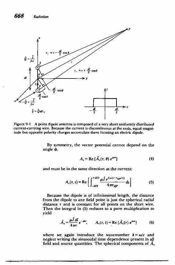
The simplest building block for a transmitting antenna is that of a uniform current flowing along a conductor of incremental length dl as shown in Figure 9-1. We assume that this current varies sinusoidally with time as
i(t)=Re (fe") (1)
Because the current is discontinuous at the ends, charge must be deposited there being of opposite sign at each end [q(t)= Re (Q e")]:
i(t)= dt I=jW>Q, Z= 2 (2)
This forms an electric dipole with moment
p= q dl i (3)
If we can find the potentials and fields from this simple element, the solution for any current distribution is easily found by superposition.
668 Radiation
P
dilQ r
ro+ dIcosO
d2
di Y c0
2
Pd 2Cos2 2
Figure 9-1 A point dipole antenna is composed of a very short uniformly distributed current-carrying wire. Because the current is discontinuous at the ends, equal magnitude but opposite polarity charges accumulate there forming an electric dipole.
By symmetry, the vector potential cannot depend on the angle 4,
A. = Re [A. (r, 0) ei. (4)
and must be in the same direction as the current:
A,(r, t)= Re d1/2 ifeiE-O-rg40) dz] (5) -1+2 4 rrQp
Because the dipole is of infinitesimal length, the distance from the dipole to any field point is just the spherical radial distance r and is constant for all points on the short wire. Then the integral in (5) reduces to a pure multiplication to yield
= dIe~5kr, A.(r, t)= Re [A.(r) ej""] (6)1
47rr
where we again introduce the wavenumber k = wo/c and neglect writing the sinusoidal time dependence present in all field and source quantities. The spherical components of A,

= V , E(r, t)= Re [E(r, 0) e""']
Radiationfrom Point Dipoles 669
are (i2 = i, cos 0 - i sin 0):
A= Azcoso, Ae=-A sinO, A.=0 (7)
Once the vector potential is known, the electric and
magnetic fields are most easily found from
N= V X A, H(r, t) = Re [H(r, 0) e"]
(8)
I
Before we find these fields, let's examine an alternate approach.
9-2-2 Alternate Derivation Using the Scalar Potential
It was easiest to find the vector potential for the point electric dipole because the integration in (5) reduced to a simple multiplication. The scalar potential is due solely to the opposite point charges at each end of the dipole,
V=- -(9)4ire ( r, r_
where r+ and r- are the distances from the respective dipole charges to any field point, as shown in Figure 9-1. Just as we found for the quasi-static electric dipole in Section 3-1-1, we cannot let r+ and r_ equal r as a zero potential would result. As we showed in Section 3-1-1, a first-order correction must be made, where
dl r+~r--cos 8
(10)dl
r_ - r +- cos 02
so that (9) becomes
S ejk (dL/2) cos 0 ---jk(dL/2) cos 6
A rer dl /e dl )(11)I Io1+-cos8 2 r ) 2r
Because the dipole length dl is assumed much smaller than the field distance r and the wavelength, the phase factors in the exponentials are small so they and the I/r dependence in the denominators can be expanded in a first-order Taylor
670 Radiation
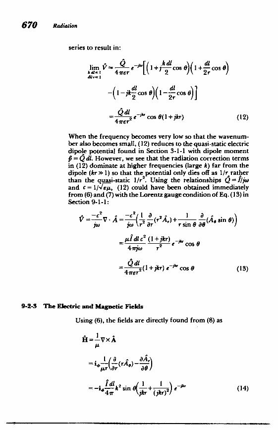
series to result in:
lim e- I+ cos 1+ cos
db K \I d1ie \ ) r ( Cos 4d Cos - -jk cdIIdc Ijr(
$ 2dl
= 2 ei' cos 0(1+jkr) (12)41rer
When the frequency becomes very low so that the wavenumber also becomes small, (12) reduces to the quasi-static electric dipole potential found in Section 3-1-1 with dipole moment f= Q dl. However, we see that the radiation correction terms in (12) dominate at higher frequencies (large k) far from the dipole (kr *1) so that the potential only dies off as 1/r rather than the quasi-static I/r2 . Using the relationships Q = I/j0 and c = 1/vj, (12) could have been obtained immediately from (6) and (7) with the Lorentz gauge condition of Eq. (13) in Section 9-1-1:
Z= (r2Z,)+ 1 (Asin 0) Y = ]w jo \r' ar r sin 8 /
p~Idlc2 (l+jkr) _~ = d 2 e cos0
4 rjw r2
Qdl = 2(1+* )e Cos 0 (13)
9-2-3 The Electric and Magnetic Fields
Using (6), the fields are directly found from (8) as
Hi= VxA
MA S - ae ,
-i-- k2 sin I-+- I e (14)41r likr (jkr)2)
Radiationfrom PointDipoles 671
E=. VXH
(j\ sin )i, - -(rao)iotoE r sin 0 aO r ar
Vi[cosO I + 1) idlk2 /;r1 1~-l k 2 41r E r s jkr)2+ (jkr)
+i, sin --- + + I e-I (15)(15)Ien jkr (Jkr)2 (jkr) e
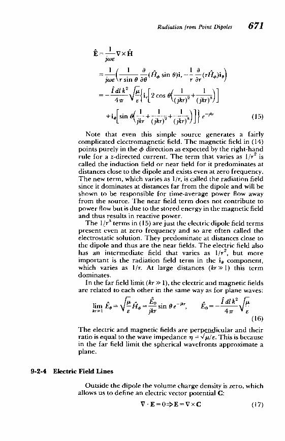
Note that even this simple source generates a fairly complicated electromagnetic field. The magnetic field in (14) points purely in the < direction as expected by the right-hand rule for a z-directed current. The term that varies as 1/r2 is called the induction field or near field for it predominates at distances close to the dipole and exists even at zero frequency. The new term, which varies as 1/r, is called the radiation field since it dominates at distances far from the dipole and will be shown to be responsible for time-average power flow away from the source. The near field term does not contribute to power flow but is due to the stored energy in the magnetic field and thus results in reactive power.
The 1/r3 terms in (15) are just the electric dipole field terms present even at zero frequency and so are often called the electrostatic solution. They predominate at distances close to the dipole and thus are the near fields. The electric field also has an intermediate field that varies as I/r 2, but more important is the radiation field term in the io component, which varies as I/r. At large distances (kr > 1) this term dominates.
In the far field limit (kr >> 1), the electric and magnetic fields are related to each other in the same way as for plane waves:
o-Id k2A = O sin 0 elim E0 kr>1 e jkr 41r
(16)
The electric and magnetic fields are perpendicular and their ratio is equal to the wave impedance 1= Vi7I. This is because in the far field limit the spherical wavefronts approximate a plane.
9-2-4 Electric Field Lines
Outside the dipole the volume charge density is zero, which allows us to define an electric vector potential C:
V - E = 0>E = V x C (17)
672 Radiation
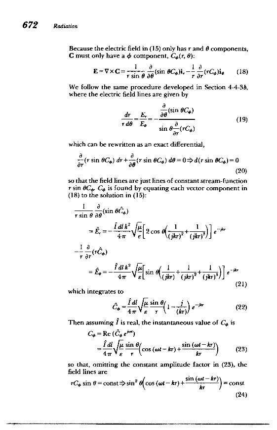
Because the electric field in (15) only has r and 0 components, C must only have a <0 component, Co(r, 0):
E = VX C= -- (sin 6C)i,-- -(rCO)i (18)r sin 08B r Or
We follow the same procedure developed in Section 4-4-3b, where the electric field lines are given by
- (sin BC,)dr = E, = 6
rdB Ee sn0a (19))sin B-(rC,)Or which can be rewritten as an exact differential,
(r sin 0C) dr + (r sin BC,) dO =0 > d(r sin C4,) = 0
(20)
so that the field lines are just lines of constant stream-function r sin BC,. C, is found by equating each vector component in (18) to the solution in (15):
I a (sin C,6)r -sin0Es
=E,=i cCos t e+ to4T r (jkr))(jkr"
(21I da
' 4si(s (-kr) (kr / (2))
=E_=-isin + + - -kr
(21) which integrates to
0 d=ZL sin0 1- e~-jk' (22)4r iTT_ r ( (kr))
Then assuming f is real, the instantaneous value of Cs is
C,= Re (C06 ej")
fd ,sn 0cos (wt - kr) + si (t-k) (23)41r E r k
so that, omitting the constant amplitude factor in (23), the field lines are
rC, sin 0 = const =sins2 cos (wt - kr) + sn(tkr = const
(24)

0
s
sin2 0 [cos kr - s =const
ywt = 0 wt 2Electrostatic
(a) dipole field solution (b)
Figure 9-2 The electric field lines for a point electric dipole at wt =0 and t = 7r/2.
674 Radiation
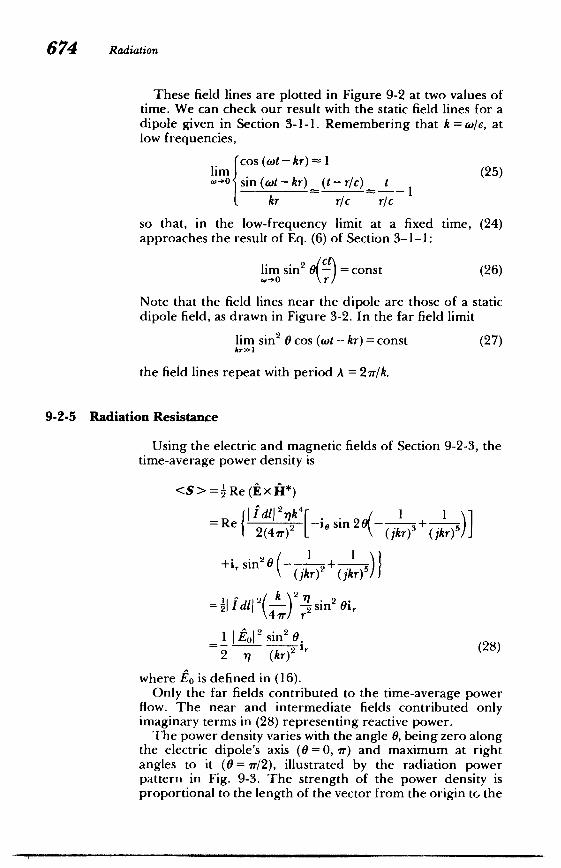
These field lines are plotted in Figure 9-2 at two values of time. We can check our result with the static field lines for a dipole given in Section 3-1-1. Remembering that k = w/c, at low frequencies,
lrn cos (wt - kr) 1 (25)-0 sin (cot - kr) (t - rc) t
kr r/c r/c
so that, in the low-frequency limit at a fixed time, (24) approaches the result of Eq. (6) of Section 3-1-1:
lim sin 2 0 -, = const (26)
Note that the field lines near the dipole are those of a static dipole field, as drawn in Figure 3-2. In the far field limit
lim sin 2 0 cos (ot - kr)= const (27)kr,l
the field lines repeat with period A = 27r/k.
9-2-5 Radiation Resistance
Using the electric and magnetic fields of Section 9-2-3, the time-average power density is
<S >=2'Re (Ex*)
= _____rk 1 + -
2(4 7r)2 s 7(jkr)+ (jkr) Re 11fdl2-q4[i, sin 2 +
+i, sin*20+ ( jkr)2 (jkr))
1 \ZoI sin 0. (28)2 q (k 2 Ir
where Zo is defined in (16). Only the far fields contributed to the time-average power
flow. The near and intermediate fields contributed only imaginary terms in (28) representing reactive power.
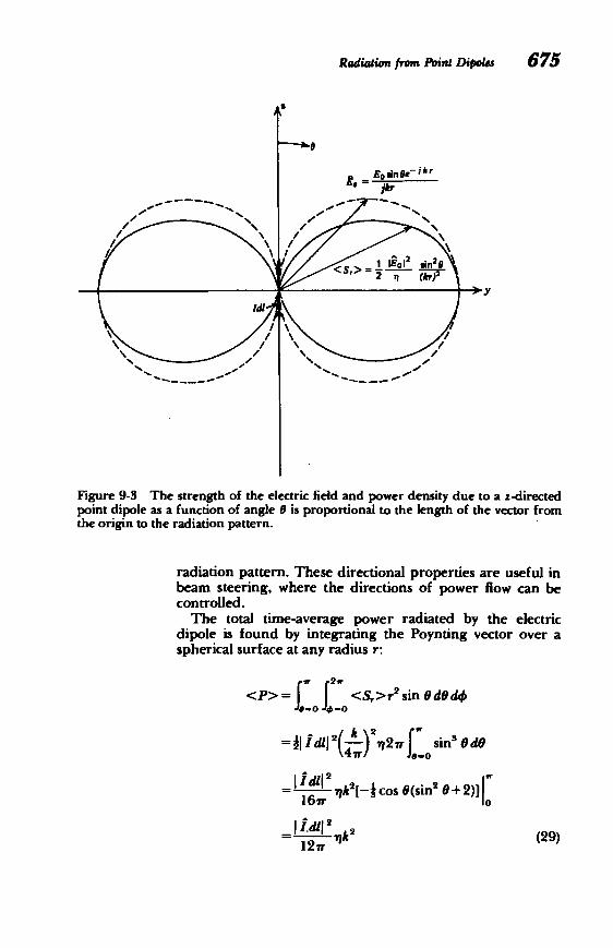
The power density varies with the angle 0, being zero along the electric dipole's axis (0 = 0, 7r) and maximum at right angles to it (0 = 7r/2), illustrated by the radiation power pattern in Fig. 9-3. The strength of the power density is proportional to the length of the vector from the origin tG the
Radiation from Point DiiJOks 675
II
9
Figure 9-3 The strength of the electric field and power density due to a z-directed point dipole as a function of angle (J is proportional to the length of the vector from the origin to the radiation pattern.
radiation pattern. These directional properties are useful in beam steering, where the directions of power Row can be controlled.
The total time-average power radiated by the electric dipole is found by integrating the Poynting vector over a spherical surface at any radius r:
(29)
676 Radiation
As far as the dipole is concerned, this radiated power is lost in the same way as if it were dissipated in a resistance R,
<> |2 R (30)
where this equivalent resistance is called the radiation resistance:
( 3d)2 k-= (31)67r 3 \A/ A
In free space 'qo=N/o/Eo- 1207r, the radiation resistance is
Ro=807r2( 2 (free space) (32)
These results are only true for point dipoles, where dl is much less than a wavelength (dl/A< 1). This verifies the validity of the quasi-static approximation for geometries much smaller than a radiated wavelength, as the radiated power is then negligible.
If the current on a dipole is not constant but rather varies with z over the length, the only term that varies with z for the vector potential in (5) is I(z):
+d1/2 ld(z) e -kr'p [ Ae-jkro +dI/2 A,(r)= Re / dz Re I(z)dz]
fd42 irr-p 4rQp /2 (33)
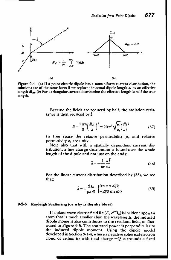
where, because the dipole is of infinitesimal length, the distance rQp from any point on the dipole to any field point far from the dipole is essentially r, independent of z. Then, all further results for the electric and magnetic fields are the same as in Section 9-2-3 if we replace the actual dipole length dl by its effective length,
1 +dL/2 dleff=- I(z)dz (34)
10 d/2
where Zo is the terminal current feeding the center of the dipole.
Generally the current is zero at the open circuited ends, as for the linear distribution shown in Figure 9-4,
_Io(l1-2z/d1), 0:5 z 54l2 IZ= Io(1+2z/dl), -d1/2:5z-0(5
so that the effective length is half the actual length:
deff- 1(z)dz= (36) 1I0 02 2
Radiation from PointDipoles 677
z Pz
0 r vo
dieff = dl2
d - -d/2 d1d2 1
)dles = d1/2 (z)dz -d1/2
x
(a) (b)
Figure 9-4 (a) If a point electric dipole has a nonuniform current distribution, the solutions are of the same form if we replace the actual dipole length dl by an effective length dl.ff. (b) For a triangular current distribution the effective length is half the true length.
Because the fields are reduced by half, the radiation resistance is then reduced by :
R= =201r2 (37)
In free space the relative permeability /A, and relative permittivity e, are unity.
Note also that with a spatially dependent current distribution, a line charge distribution is found over the whole length of the dipole and not just on the ends:
- i diA=- (38)jo> dz
For the linear current distribution described by (35), we see that:
S2Io Oszsdl/2A =5 z(39)jodl -dl/2 :z50
9-2-6 Rayleigh Scattering (orwhy is the sky blue?)
If a plane wave electric field Re [Eo e"*i.] is incident upon an atom that is much smaller than the wavelength, the induced dipole moment also contributes to the resultant field, as illustrated in Figure 9-5. The scattered power is perpendicular to the induced dipole moment. Using the dipole model developed in Section 3-1-4, where a negative spherical electron cloud of radius RO with total charge -Q surrounds a fixed

E =Re(Eoe J9)
S incident
S scAttered a
. . ..
!T.~
(a)
rgE
(b>
Figure 9-5 An incident electric field polarizes dipoles that then re-radiate their energy primarily perpendicular to the polarizing electric field. The time-average scattered power increases with the fourth power of frequency so shorter wavelengths of light are scattered more than longer wavelengths. (a) During the daytime an earth observer sees more of the blue scattered light so the sky looks blue (short wavelengths). (b) Near sunset the light reaching the observer lacks blue so the sky appears reddish (long wavelength).
678
Radiation from Point Dipoles 679
positive point nucleus, Newton's law for the charged cloud with mass m is:
d 2 x 2 QEo j. 2 Q2 + Wx=-Re e 1 , (=W3 (40)d( M 4,rEmRo
The resulting dipole moment is then
Q2 Eo/m p = 2 2 (41)
(00 -t
where we neglect damping effects. This dipole then re-radiates with solutions given in Sections 9-2-1-9-2-5 using the dipole moment of (41) (Idl-jop). The total time-average power radiated is then found from (29) as
< =_ir1 w47(Q2Eo/m)22 2 2<P>= c = 12T 2 o- (42)12rc 12rc _0 7
To approximately compute wo, we use the approximate radius of the electron found in Section 3-8-2 by equating the energy stored in Einstein's relativistic formula relating mass to energy:
2 3Q2 3Q 2
mc = -> ii-mc 1.69x 10- 5m(43)
Then from (40)
5/3207Tmc 3 '
3Q2Co ~2.3 X 10²³ radian/sec (44)
is much greater than light frequencies (to 1015) so that (42) becomes approximately
Jim <>= 7 Q2Eow 2 lim <P> (45)wO>> 127r( mcw
This result was originally derived by Rayleigh to explain the blueness of the sky. Since the scattered power is proportional to (04, shorter wavelength light dominates. However, near sunset the light is scattered parallel to the earth rather than towards it. The blue light received by an observer at the earth is diminished so that the longer wavelengths dominate and the sky appears reddish.
9-2-7 Radiation from a Point Magnetic Dipole
A closed sinusoidally varying current loop of very small size flowing in the z = 0 plane also generates radiating waves. Because the loop is closed, the current has no divergence so

680 Radiation
that there is no charge and the scalar potential is zero. The vector potential phasor amplitude is then
A(r)= f - eiTQp dl (46)4
lrro
We assume the dipole to be much smaller than a wavelength, k(rQp-r)« 1, so that the exponential factor in (46) can be linearized to
lim e-ik'Qp = elk'e-('Qp-') ==eir[ -jk(rQp-r)]
(47)
Then (46) reduces to
A(r)=f e--iQ+jkr-) di 47r \rQP
=e* - -! di-jk4 7r rop
dl jk f dl (48) =---e k(1+jkr) 4ir\ J rQP J /
where all terms that depend on r can be taken outside the integrals because r is independent of dl. The second integral is zero because the vector current has constant magnitude and flows in a closed loop so that its average direction integrated over the loop is zero. This is most easily seen with a rectangular loop where opposite sides of the loop contribute equal magnitude but opposite signs to the integral, which thus sums to zero. If the loop is circular with radius a,
2w2 21r-si idt= higa d4 -> i, d4= (-sin i. + cos Oi,) dO =0
(49)
the integral is again zero as the average value of the unit vector i# around the loop is zero.
The remaining integral is the same as for quasi-statics except that it is multiplied by the factor (1+ jkr) e ''. Using the results of Section 5-5-1, the quasi-static vector potential is also multiplied by this quantity:
AM sin 0(1+ jkr) eik*'i,, A f dS (50)47rr2
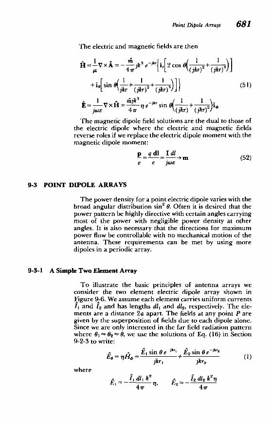
Point Dipole Arrays 681
The electric and magnetic fields are then
f=-VxA= jk e-ik' 2Cos 2+ s LOS ~ (jkr)2 (jkr) J
[ 1 1 1\1 +1e[slnl--+ +2+ (51)s
jkr (jkr)+(jkr)-"7
E1 xN= 7e--krsin0 +GjWE 4r (jkr) (jkr)Y/
The magnetic dipole field solutions are the dual to those of the electric dipole where the electric and magnetic fields reverse roles if we replace the electric dipole moment with the magnetic dipole moment:
p = dl Idl -= --- - ->m(52)
e e )oe
9-3 POINT DIPOLE ARRAYS
The power density for a point electric dipole varies with the broad angular distribution sin2 0. Often it is desired that the power pattern be highly directive with certain angles carrying most of the power with negligible power density at other angles. It is also necessary that the directions for maximum power flow be controllable with no mechanical motion of the antenna. These requirements can be met by using more dipoles in a periodic array.
9-3-1 A Simple Two Element Array
To illustrate the basic principles of antenna arrays we consider the two element electric dipole array shown in Figure 9-6. We assume each element carries uniform currents I and i2 and has lengths d1l and d12 , respectively. The elements are a distance 2a apart. The fields at any point P are given by the superposition of fields due to each dipole alone. Since we are only interested in the far field radiation pattern where 01 2= 0, we use the solutions of Eq. (16) in Section 9-2-3 to write:
E, sin Oe-l+E2 sin 0 e-rz'2
jkri jkr2 where
-P 1 dl,k2 P 12 d12 k E=r , = 4ir4
E2

682 Radiation
Z
2 2r2= [r + a -2arcos(ir -t )1
2 r + asin 0cos
2a 2
2 2[r + a -2arcos 112 J r -asinOcoso
cos =i,. -i sin0coso
-Jd, a
Figure 9-6 The field at any point P due to two-point dipoles is just the sum of the fields due to each dipole alone taking into account the difference in distances to each dipole.
Remember, we can superpose the fields but we cannot superpose the power flows.
From the law of cosines the distances r, and are relatedr2
as
r2 =[r2 + a2 -2ar cos (7-_6)] 2 =[r 2 + a2 +2arcos e]
r = [r2 + a 2-2ar cos e]112
where 6 is the angle between the unit radial vector i, and the x axis:
cos = ir = sin 0 cos 4
Since we are interested in the far field pattern, we linearize (2) to
r2 r2 +2 r +- r sin 0cos 4]r + a sin0 cos4
lim r a (3)
r, -- r 1+-( 2 sin 0 Cos ~r - a sin 0 cos 2 r2 r
In this far field limit, the correction terms have little effect in the denominators of (1) but can have significant effect in the exponential phase factors if a is comparable to a wavelength so that ka is near or greater than unity. In this spirit we include the first-order correction terms of (3) in the phase
2
Point Dipole Arrays 683
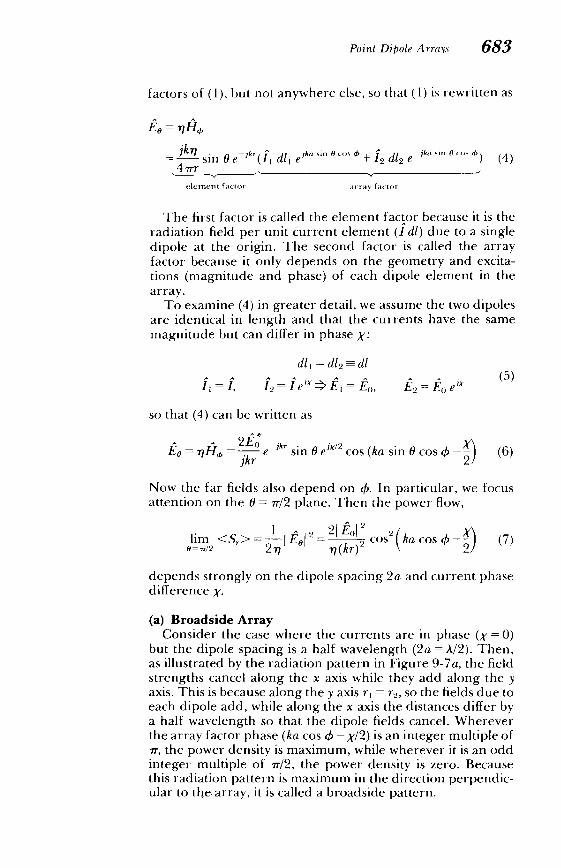
factors of (1), but not anywhere else, so that (1) is rewritten as
jkr1 sin 6 e-k (ij d11 ejk' s"O- + f, d1 2 e-'k" 0""'t) (4) 4 7rr
elemret factor array factor
The first factor is called the element factor because it is the radiation field per unit current element (f dl) due to a single dipole at the origin. The second factor is called the array factor because it only depends on the geometry and excitations (magnitude and phase) of each dipole element in the array.
To examine (4) in greater detail, we assume the two dipoles are identical in length and that the currents have the same magnitude but can differ in phase x:
dl, = dl2 =dl
I= =, = Ie'x =E0, E= oe" (5)fEi
so that (4) can be written as
2Le r sin 6e j2 cos (ka sin 6cos q -- (6) = f jkr 2
Now the far fields also depend on 0. In particular, we focus attention on the 6 = 7r/2 plane. Then the power flow,
lim <Sr>= \I = 2 cos ka cos (7)=(/2 2kr) (24
depends strongly on the dipole spacing 2a and current phase difference X.
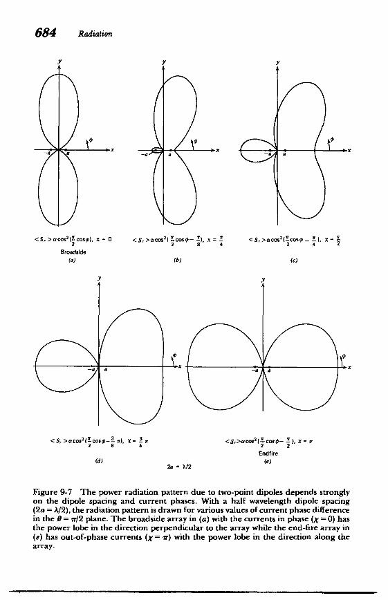
(a) Broadside Array Consider the case where the currents are in phase (X = 0)
but the dipole spacing is a half wavelength (2a = A/2). Then, as illustrated by the radiation pattern in Figure 9-7a, the field strengths cancel along the x axis while they add along the y axis. This is because along the y axis r, = r2 , so the fields due to each dipole add, while along the x axis the distances differ by a half wavelength so that the dipole fields cancel. Wherever the array factor phase (ka cos 0 -x/ 2 ) is an integer multiple of 7T, the power density is maximum, while wherever it is an odd integer multiple of Tr/2, the power density is zero. Because this radiation pattern is maximum in the direction perpendicular to the. array, it is called a broadside pattern.
684 Radiation
Y
Al) 10ox3. x x-a -a a a<1 <S, >aCOs2( !cos$j), ), x = 1! <S,>OcOs2(!cos 0 I ), X =
2 2 8 4 2 c 2 X = 0 <S,> cos2 cos$-
Broadside (a) (b) (C)
r__ r-) -a a -a a
<S,>acos2! cos0_- f), x = -w <S,>aCO2 I COS0_, X = 2 8 4 2 2
Endfire (d) (e)
2a - A/2
Figure 9-7 The power radiation pattern due to two-point dipoles depends strongly on the dipole spacing and current phases. With a half wavelength dipole spacing (2a = A/2), the radiation pattern is drawn for various values of current phase difference in the 6= ir/2 plane. The broadside array in (a) with the currents in phase (X =0) has the power lobe in the direction perpendicular to the array while the end-fire array in (e) has out-of-phase currents (x = 7r) with the power lobe in the direction along the array.
Point Dipole Arrays 685
(b) End-fire Array If, however, for the same half wavelength spacing the cur
rents are out of phase (X = 1r), the fields add along the x axis but cancel along the y axis. Here, even though the path lengths along the y axis are the same for each dipole, because the currents are out of phase the fields cancel. Along the x axis the extra 7r phase because of the half wavelength path difference is just canceled by the current phase difference of ir so that the fields due to each dipole add. The radiation pattern is called end-fire because the power is maximum in the direction along the array, as shown in Figure 9-7e.
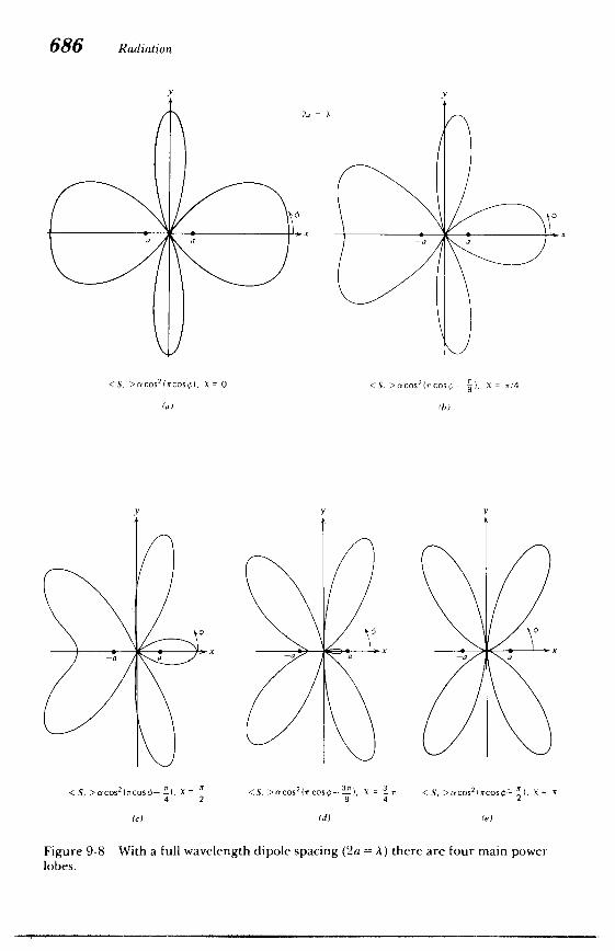
(c) Arbitrary Current Phase For arbitrary current phase angles and dipole spacings, a
great variety of radiation patterns can be obtained, as illustrated by the sequences in Figures 9-7 and 9-8. More power lobes appear as the dipole spacing is increased.
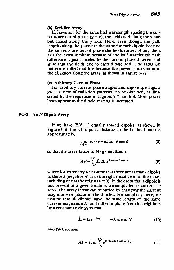
9-3-2 An N Dipole Array
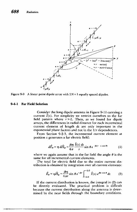
If we have (2N+ 1) equally spaced dipoles, as shown in Figure 9-9, the nth dipole's distance to the far field point is approximately,
lim rn~r-nasinocoso (8)
so that the array factor of (4) generalizes to
AF= +NY in dl.e1sinb0"cos"" (9)-N
where for symmetry we assume that there are as many dipoles to the left (negative n) as to the right (positive n) of the z axis, including one at the origin (n = 0). In the event that a dipole is not present at a given location, we simply let its current be zero. The array factor can be varied by changing the current magnitude or phase in the dipoles. For simplicity here, we assume that all dipoles have the same length dl, the same current magnitude 1o, and differ in phase from its neighbors by a constant angle Xo so that
In = Io e-1"0, --N nc n s N (10)
and (9) becomes
+ N AF = o dl Y, dn(kAasin 0 cOs-xo) (1
-N
686 Radiation
y y 2
a
r-
<S, >aCOS 2
(7 COs),
(a)
-
X = 0 <S, >ocos 2
(mcoso
(b)
-a
LiK '), X = /4
x a
x 0
0 -0
2 2 < S, > cos (cos@- (I , C= ) <S, >acos (ircos$- 3), X = <S, >Ucos2( 7 cos ), X =
42
(C) (d) (e)
Figure 9-8 With a full wavelength dipole spacing (2a =A) there are four main power lobes.
Point Dipole Arrays 687
Defining the parameter
3=eej(ka sinecos #Xo) (12)
the geometric series in (11) can be written as
S= -N P"#-N + -N+l. I 4 +-24 +- I 2+
+ ,9N 1 + N (13)
If we multiply this series by ( and subtract from (13), we have
S(1 (3) -N _ N+1 (14)
which allows us to write the series sum in closed form as
N+1 v(N+1/2)_(N+1/2)--Ns= 1--3 = 3-1/2l_/2
sin [(N+ )(ka sin 0 cos 4)-Xo)] (15) sin [-(ka sin 6 cos 4 -Xo)I
In particular, we again focus on the solution in the 0= 7r/2
plane so that the array factor is
AF= Io dl sin [(N+)(ka cos 4X-o)] (16)sin [A(ka .cos 4 - Yo)]
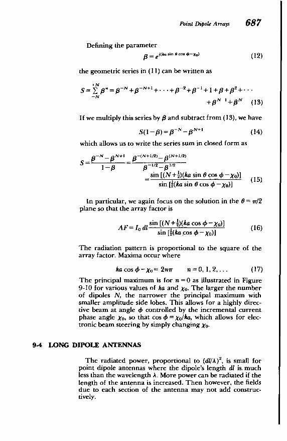
The radiation pattern is proportional to the square of the array factor. Maxima occur where
ka cos 4-Xo= 2nir n=0, 1,2,... (17)
The principal maximum is for n =0 as illustrated in Figure 9-10 for various values of ka and Xo. The larger the number of dipoles N, the narrower the principal maximum with smaller amplitude side lobes. This allows for a highly directive beam at angle 4 controlled by the incremental current phase angle Xo, so that cos 4 = Xo/ka, which allows for electronic beam steering by simply changing Xo.
9-4 LONG DIPOLE ANTENNAS
The radiated power, proportional to (dli/A )2, is small for point dipole antennas where the dipole's length dl is. much less than the wavelength A. More power can be radiated if the length of the antenna is increased. Then however, the fields due to each section of the antenna may not add constructively.
= e
y
688 Radiation
n =-N
2
n -s3 n s n
0y
3 ddI3
n =
current I(z). For simplicity we restrict ourselves to the far field pattern where r ~'L. Then, as we found for dipole arrays, the differences in radial distance for each incremental current element of length dz are only important in the exponential phase factors and not in the /r dependences.
From Section 9-2-3, the incremental current element at position z generates a far electric field:
=jk'q 1(z ) dzdE0 dI, A= sin eA(r-cos 0) 1)-
41T r
where we again assume that in the far field the angle 6 is the same for all incremental current elements.
The total far electric field due to the entire current distribution is obtained by integration over all current elements:
E =- sin OC z)Uel cos dz (2)
If the current distribution is known, the integral in (2) can be directly evaluated. The practical problem is difficult because the current distribution along the antenna is determined by the near fields through the boundary conditions.
Long Dipole Antennas 689
a = /
N= 2 N=1
N= 3N= 1 N= 2 X0= /2
Xo = 0 x
a = /2
N= 1 N= 2 N= 1 N =2 Xo = 0 X = m/2
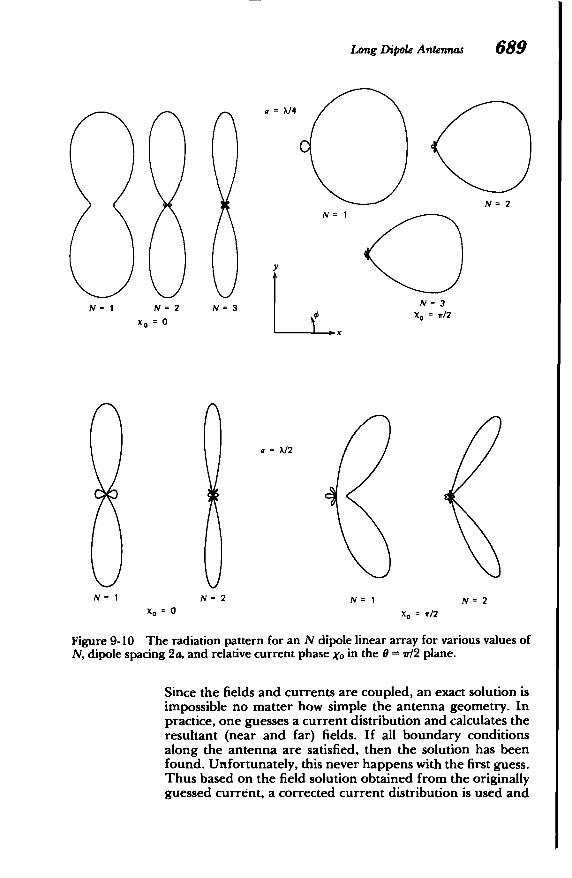
Figure 9-10 The radiation pattern for an N dipole linear array for various values of N, dipole spacing 2a, and relative current phase Xo in the 6 = ir/2 plane.
Since the fields and currents are coupled, an exact solution is impossible no matter how simple the antenna geometry. In practice, one guesses a current distribution and calculates the resultant (near and far) fields. If all boundary conditions along the antenna are satisfied, then the solution has been found. Unfortunately, this never happens with the first guess. Thus based on the field solution obtained from the originally guessed current, a corrected current distribution is used and

690 Radiation
y
N= 1 N 1
Xo= 0
N= 2N= 2
xo = 0 X0
Figure 9-10
the resulting fields are again calculated. This procedure is numerically iterated until convergence is obtained with self-consistent fields and currents.
9-4-2 Uniform Current
A particularly simple case is when f(z)= fo is a constant. Then (2) becomes:
jkE0 sin Oe o +u " 47rr E/2
47re jkzcos 6 L2
4 -7rI k CS 0 1kL/
1071 tan 4t7rr
e 2j sinL
kL -cos
\2 9) (3)
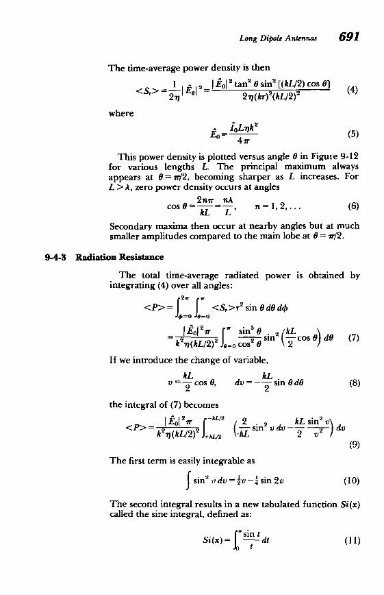
Long Dipole Antennas 691
The time-average power density is then
<S'>= i1 IjI2 1 2 tanJ20 sin2 [(kL/2) cos 0] (4) 2 1(kr)2 (kL/2)2
27
where
i-E= foLqk-"(5fLk 2 (5)47r
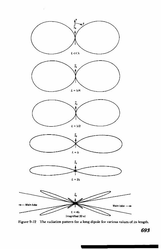
This power density is plotted versus angle 6 in Figure 9-12 for various lengths L. The principal maximum always appears at 6= ir/2. becoming sharper as L increases. For L >A, zero power density occurs at angles
Cos = 2 =n , n=2,... (6)kL L
Secondary maxima then occur at nearby angles but at much smaller amplitudes compared to the main lobe at 6= 7r/2.
9-4-3 Radiation Resistance
The total time-average radiated power is obtained by
integrating (4) over all angles:
<P>= <S,>r2 sin 0 dO d4
IZo| 2 r " sin3 0 2 kL 6) dO (7) 2k2 q(kL/2)2 J=o cos 6si s (
If we introduce the change of variable,
kL kL v = cos 0, dv= Usin 0 d6 (8)
2 '2
the integral of (7) becomes
<P>-= i -WI 2 sin2 vdv kL sinl2v2dvkP2k +Al/2 \-kL 2 v(kL/2)2
(9)
The first term is easily integrable as
fsin 2 dv = -{ 4vsin 2v (10)
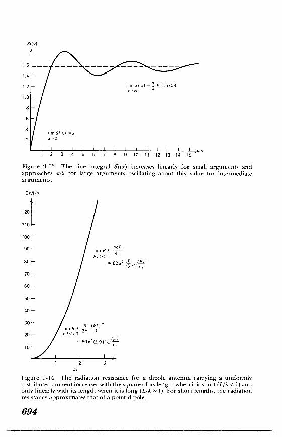
The second integral results in a new tabulated function Si(x) called the sine integral, defined as:
Si(x)= {sintdt (II)ft

692 Radiation
P
L zcosO z
, (a) 1(z)
z
Wb
x
Figure 9-11 (a) For a long dipole antenna, each incremental current element at coordinate z is at a slightly different distance to any field point P. (b) The simplest case study has the current uniformly distributed over the length of the dipole.
which is plotted in Figure 9-13. Then the second integral in (9) can be expanded and integrated by parts:
sin 2 v (I -cos 2v) dv fV 2v2
= _ cos 2v dv22v 2V
I cos2v( sin 2vd(2v) 2v 2v 2v
= +cos 2v+Si(2v) (12)2v 2v
Then evaluating the integrals of (10) and (12) in (9) at the upper and lower limits yields the time-average power as:
<P>= +cos kL -2 + kLSi(kL) (13)k2k (kL/2) 2 kL
where we used the fact that the sine integral is an odd function Si(x)= -Si(x).
Using (5), the radiation resistance is then
2<P> 71 sin kL R ^ 2 = + cos kL -2+kLSi(kL) (14)
|Io|2 27r kL
10
L <<
( O
FeTL Oxn
69 C)L = X12
70
C =2
10
-<-]* Main:1obe Main lobe-31
(magnified 20 x)
Figure 9-12 The radiation pattern for a long dipole for various values of its length.
693
Si(x)
/
1.6
1.4
1.2 lim Si(x) -1.5708
-- '01.0
.8
.6
.4 lim Si(x) -x x'O.2
1 2 3 4 5 6 7 8 9 10 11 12 13 14 15
Figure 9-13 The sine integral Si(x) increases linearly for small arguments and approaches ir/2 for large arguments oscillating about this value for intermediate arguments.
21rR/77
120
110
100
90 lim R r7kL kI>> 1 4
80 =60T2(L V
70
60
50
- I40
30 (UL) 2 lrn R 27 3
- kl«120
80 r 2(L A)2
10.
1 2 3 kL
Figure 9-14 The radiation resistance for a dipole antenna carrying a uniformly distributed current increases with the square of its length when it is short (L/A < 1) and only linearly with its length when it is long (L/A > 1). For short lengths, the radiation resistance approximates that of a point dipole.
694
Problems 695
which is plotted versus kL in Fig. 9-14. This result can be checked in the limit as L becomes very small (kL < 1) since the radiation resistance should approach that of a point dipole given in Section 9-2-5. In this short dipole limit the bracketed terms in (14) are
sin kL (kL)2
kL 6
knkL II coskU I(kL )2 ((15) 2
kLSi(kL) (kL)2
so that (14) reduces to
lim R -v (kL )2 2rn L 2 2 (L (16)8 02 r 3 3 A A Er
which agrees with the results in Section 9-2-5. Note that for large dipoles (kL >> 1), the sine integral term dominates with Si(kL) approaching a constant value of 7r/2 so that
lim R _- = 60 r2 L (17)kL 1 4 Er A
PROBLEMS
Section 9-1 1. We wish to find the properties of waves propagating within a linear dielectric medium that also has an Ohmic conductivity o-.
(a) What are Maxwell's equations in this medium? (b) Defining vector and scalar potentials, what gauge
condition decouples these potentials? (c) A point charge at r = 0 varies sinusoidally with time as
Q(t) = Re (Q e'"). What is the scalar potential? (d) Repeat (a)-(c) for waves in a plasma medium with
constitutive law
aSf= w eE at
2. An infinite current sheet at z = 0 varies as Re [K0 e - il.
(a) Find the vector and scalar potentials. (b) What are the electric and magnetic fields?

MIT OpenCourseWarehttp://ocw.mit.edu
Resource: Electromagnetic Field Theory: A Problem Solving ApproachMarkus Zahn
The following may not correspond to a particular course on MIT OpenCourseWare, but has beenprovided by the author as an individual learning resource.
For information about citing these materials or our Terms of Use, visit: http://ocw.mit.edu/terms.the
/


