71

Physics II
Electromagnetism and Optics
Charudatt Kadolkar
Indian Institute of Technology Guwahati
Jan 2009

Physics II Syllabus
Vector Calculus: Gradient, Divergence and Curl. Line, Surface, and Volume integrals. Gauss'sdivergence theorem and Stokes' theorem in Cartesian, Spherical polar, and Cylindrical polar coordinates.Dirac Delta function.
Electrodynamics: Coulomb's law and Electrostatic �eld, Fields of continuous charge distributions.Gauss's law and its applications. Electrostatic Potential. Work and Energy. Conductors. Capacitors.Laplace's equation. Method of images. Dielectrics. Polarization. Bound Charges. Energy in dielectrics.Boundary conditions.
Lorentz force. BiotSavart and Ampere's laws and their applications. Vector Potential. Force and torqueon a magnetic dipole. Magnetic materials. Magnetization, Bound currents. Boundary conditions.Motional EMF, Ohm's law. Faraday's law. Lenz's law. Self and Mutual inductance. Energy stored inmagnetic �eld. Maxwell's equations.
Optics: Huygens' principle. Young's experiment. Superposition of waves. Concepts of coherencesources. Interference by division of wavefront. Fresnel's biprism, Phase change on re�ection. Lloyd'smirror. Interference by division of amplitude. Parallel �lm. Film of varying thickness. Colours of thin�lms. Newton's rings. The Michelson interferometer. Fraunhofer di�raction. Single slit, double slit andN-slit patterns. The di�raction grating.

Reading Material
I Textbooks
1. D. J. Gri�ths, Introduction to Electrodynamics, Prentice-Hall (1995).2. F. A. Jenkins and H. E. White, Fundamental of Optics, McGraw-Hill,
(1981).
I References:
1. Feynman, Leighton, and Sands, The Feynman Lectures on Physics,Vol. II, Norosa Publishing House (1998).
2. I. S. Grant and W. R. Phillips, Electromagnetism, John Wiley, (1990).3. E. Hecht, Optics, Addison-Wesley, (1987).

Vector Analysis
MA101: Mathematics IVector functions of one variable and their derivatives. Functions of severalvariables, partial derivatives, chain rule, gradient and directional derivative.Tangent planes and normals. Maxima, minima, saddle points, Lagrangemultipliers, exact di�erentials.Repeated and multiple integrals with application to volume, surface area,moments of inertia. Change of variables. Vector �elds, line and surfaceintegrals. Green's, Gauss' and Stokes' theorems and their applications.

Scalar And Vector Quantities
Physical Quantity
Observables, which can be measured and represented by numbers, are calledphysical quantities.
Some Examples
I mass of a body,
I volume of a body,
I temperature at a point etc.
Some More Examples
I position of a particle,
I electric �eld at a point
I size of a cuboid,
I thermodynamic state (ρ,P,T )
Scalar quantities have magnitude and vector quantities have magnitude as wellas direction.
Vectors are represented by three real numbers.
Is a physical quantity represented by three numbers, a vector?

Alternate De�nition: Vector Quantities
Two observers with di�erent coordinate systems are shown in the �gure.
X
Y
P
Α
x
y
X’
Y’
x’
y’
The coordinates of a point P
x ′ = x cosα+ y sinα
y ′ = −x sinα+ y cosα[x ′
y ′
]=
[cosα sinα− sinα cosα
] [x
y
]
X
Y
Α
A
X’
Y’
Components of A in two frames arerelated by[
A′x
A′y
]=
[cosα sinα− sinα cosα
] [Ax
Ay
]

Alternate De�nition: Vector Quantities
De�nition
Suppose a physical quantity A is represented by n components in n-dimensionalspace. If, under a coordinate transformation, the components of A transform inthe same way as coordinates, then the physical quantity A is said to be a vector
quantity.
Scalar quantities donot depend on the coordinate transformations.
size of cuboid, a state of a thermodynamic system are not a vector quantitiesbut are collections of three scalar quantities.
Scalar And Vector Functions of One Variable
Typically, in Physics, scalar and vector quantities are functions of time.Examples are:
I Temperature of a body
I Amount of Radioactive material etc.
I Position of a particle
I Forces on a particle
We are quite familiar with scalar functions and calculus of such functions.Calculus of vector valued functions is also familiar to us.
Example
Suppose r : R→ R3 is position of a particle as a function of time. Letr (t) = x(t)x + y(t)y + z(t)z. Then, velocity of the particle is given by
v(t) =d
dtr (t) =
dx
dt(t)x +
dy
dt(t)y +
dz
dt(t)z.

Scalar and Vector Fields
While describing extended objects that �ll space or regions of space, we use�elds, that is, with each point of the space, we associate a vector or scalarproperty.
Examples are:
I Air temperature across the Earth,
I Height of a location from sea level,
I Density of a �uid,
I Force Fields (Gravitational, Electrostatic),
I Potential energy of a force �eld etc.
Mathematically, these are functions from Rm to Rn, with m > 1. If n = 1,these functions are called scalar �elds otherwise are called vector �elds.

Scalar Fields (2D)
x
y
z
f (x , y) = x2 + y2
Scalar Fields (2D)
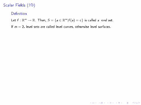
De�nition
Let f : Rm → R. Then, S = {a ∈ Rm|f (a) = c} is called a level set.
If m = 2, level sets are called level curves, otherwise level surfaces.
x
y
z
-1.5 -1 -0.5 0 0.5 1 1.5-1.5
-1
-0.5
0
0.5
1
1.5

Scalar Fields (2D)
De�nition
Let f : Rm → R. Then, S = {a ∈ Rm|f (a) = c} is called a level set.
If m = 2, level sets are called level curves, otherwise level surfaces.
x
y
z
-1.5 -1 -0.5 0 0.5 1 1.5-1.5
-1
-0.5
0
0.5
1
1.5

Scalar Fields (2D)
De�nition
Let f : Rm → R. Then, S = {a ∈ Rm|f (a) = c} is called a level set.
If m = 2, level sets are called level curves, otherwise level surfaces.
x
y
z
-1.5 -1 -0.5 0 0.5 1 1.5-1.5
-1
-0.5
0
0.5
1
1.5

Scalar Fields (2D)
De�nition
Let f : Rm → R. Then, S = {a ∈ Rm|f (a) = c} is called a level set.
If m = 2, level sets are called level curves, otherwise level surfaces.
x
y
z
-2 -1 0 1 2-2
-1
0
1
2
0
4

Scalar Fields (2D)
De�nition
Let f : Rm → R. Then, S = {a ∈ Rm|f (a) = c} is called a level set.
If m = 2, level sets are called level curves, otherwise level surfaces.
x
y
z
-2 -1 0 1 2-2
-1
0
1
2
0
4

Scalar Fields (2D)
De�nition
Let f : Rm → R. Then, S = {a ∈ Rm|f (a) = c} is called a level set.
If m = 2, level sets are called level curves, otherwise level surfaces.
x
y
z
-2 -1 0 1 2-2
-1
0
1
2
0
4

Scalar Fields (3D)
Two identical point charges at (1, 0, 0) and (−1, 0, 0). The potential in xy-plane
V (x , y , z = 0) =Q
4πε0
1√(x − 1)2 + y2
+1√
(x + 1)2 + y2
-2
0
2
-2
-1
01
2
0
2
4
6-2
-1
01
-3 -2 -1 0 1 2 3-2
-1
0
1
2

Scalar Fields (3D)
Two identical point charges at (1, 0, 0) and (−1, 0, 0). The potential in xy-plane
V (x , y , z = 0) =Q
4πε0
1√(x − 1)2 + y2
+1√
(x + 1)2 + y2
-2
0
2
-2
-1
01
2
0
2
4
6-2
-1
01
-3 -2 -1 0 1 2 3-2
-1
0
1
2

Scalar Fields (3D)
Two identical point charges at (1, 0, 0) and (−1, 0, 0). The potential in xy-plane
V (x , y , z = 0) =Q
4πε0
1√(x − 1)2 + y2
+1√
(x + 1)2 + y2
-2
0
2
-2
-1
01
2
0
2
4
6-2
-1
01
-3 -2 -1 0 1 2 3-2
-1
0
1
2
Scalar Fields (3D)
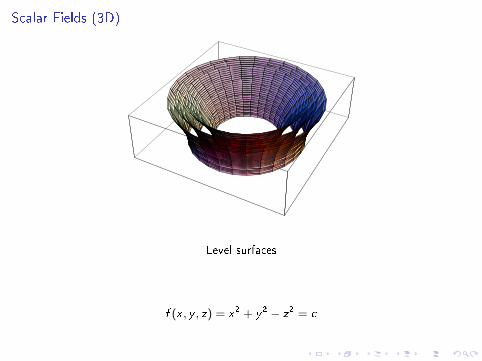
Level surfaces
f (x , y , z) = x2 + y2 − z2 = c

Vector Fields (2D)
f (x , y) = x x + y y

Vector Fields (2D)
-2 -1 1 2
-2
-1
1
2
f (x , y) = −y x + x y

Vector Fields (2D)
Two opposite point charges at (1, 0, 0) and (−1, 0, 0). The electric �eld inxy-plane
E(x , y) =Q
4πε0
((x − 1) x + y y(
(x − 1)2 + y2)3/2
− (x + 1) x + y y((x + 1)2 + y2
)3/2
)

Directional Derivative and Partial Derivatives
x
y
z
a t
f (x , y) = x2 + y2
a = (1, 0)t = (1, 1)/
√2
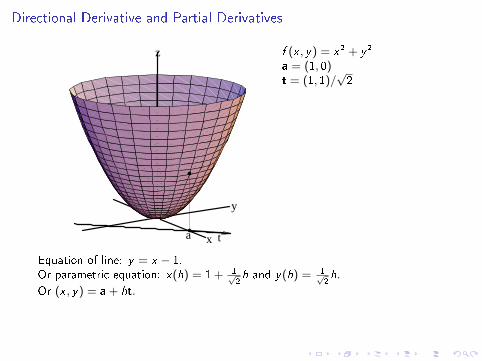
Consider function f (x , y) = x2 + y2
Directional Derivative and Partial Derivatives
x
y
z
a t
f (x , y) = x2 + y2
a = (1, 0)t = (1, 1)/
√2
Equation of line: y = x − 1.Or parametric equation: x(h) = 1 + 1√
2h and y(h) = 1√
2h.
Or (x , y) = a + ht.

Directional Derivative and Partial Derivatives
x
y
z
a t
f (x , y) = x2 + y2
a = (1, 0)t = (1, 1)/
√2
-2 -1.5 -1 -0.5 0.5h
fHhL
Write: f (h) = f (x(h), y(h)) = f (a + ht) = 1 +√2h + h2
f ′ (a; t) =df
dh(h = 0) =
√2

Directional Derivative and Partial Derivatives
x
y
z
a t
f (x , y) = x2 + y2
a = (1, 0)t = (1, 1)/
√2
-2 -1.5 -1 -0.5 0.5h
fHhL
Equation of the tangent to f (h): 1 +√2h
Equation of the tangent to f (x , y): x = 1 + h/√2, y = h/
√2, z =
√2h

Directional Derivative and Partial Derivatives
I Let f (x , y) = x2 + y2. Let a = (1, 0) and t = (1, 1)/√2 .
I Line parallel to t and passing through a:
x = 1 +1√2h and y =
1√2h.
with (x , y) = a at h = 0.
I Restriction of function f along this line:
f (h) = f (x(h), y(h)) = 1 +√2h + h2
I Directional derivative
f ′ (a; t) =df
dh(h = 0) =
√2
I Equation of the tangent to f (h): y = 1 +√2h.
I Equation of the tangent to f (x , y): x = 1 + t/√2, y = t/
√2, z =
√2t

Directional Derivative and Partial Derivatives
De�nition
Let f : R3 → R be a scalar �eld. Let a ∈ R3 be a point in space. Supposet ∈ R3 be a unit vector. Then
limh→0
f (a + ht)− f (a)
h
is called directional derivative of f at a in the direction of t and is denoted byf ′(a; t). (If the limit exists.)
The directional derivative in any one of the coordinate unit vectors, that is,either x, y or z, is also called partial derivative. Partial derivatives are usuallydenoted by
∂
∂xf (a),
∂
∂yf (a) or
∂
∂zf (a).
Example
In previous example: f (x , y) = x2 + y2 and a = (1, 0) then
∂
∂xf (a) = 2,
∂
∂yf (a) = 0.

Di�erentiability
Notion of di�erentiability
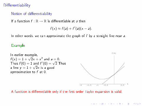
If a function f : R→ R is di�erentiable at a then
f (x) ≈ f (a) + f ′(a)(x − a).
In other words, we can approximate the graph of f by a straight line near a.
Example
In earlier example,f (x) = 1 +
√2x + x2 and a = 0.
Thus f (0) = 1 and f ′(0) =√2 Thus
a line y = 1 +√2x is a good
aprroximation to f at 0.
-2 -1.5 -1 -0.5 0.5h
fHhL
A function is di�erentiable only if the �rst order Taylor expansion is valid.

Di�erentiability
Notion of di�erentiability
If a function f : R→ R is di�erentiable at a then
f (x) ≈ f (a) + f ′(a)(x − a).
In other words, we can approximate the graph of f by a straight line near a.
Example
In earlier example,f (x) = 1 +
√2x + x2 and a = 0.
Thus f (0) = 1 and f ′(0) =√2 Thus
a line y = 1 +√2x is a good
aprroximation to f at 0.
-2 -1.5 -1 -0.5 0.5h
fHhL
A function is di�erentiable only if the �rst order Taylor expansion is valid.

Total Derivative
Di�erentiability for functions of two variables
If a function of two variables is to be di�erentiable, one must be approximateits graph by a plane rather than a line.
Example
Consider f (x , y) = x2 + y2 anda = (1, 0). Figure shows a planegiven by a functionz(x , y) = 1 + 2(x − 1). Here iscomparison
f (1.1, 0) = 1.21 z(1.1, 0) = 1.20,
f (1, 0.1) = 1.01 z(1, 0.1) = 1.00.
x
y
zf= x2
+ y2
z= 2 x-1
Total Derivative
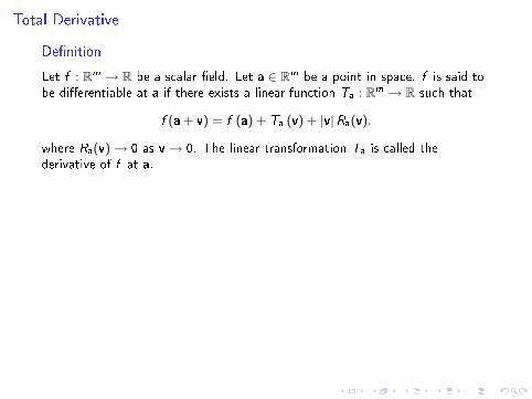
De�nition
Let f : Rm → R be a scalar �eld. Let a ∈ Rm be a point in space. f is said tobe di�erentiable at a if there exists a linear function Ta : Rm → R such that
f (a + v) = f (a) + Ta (v) + |v|Ra(v).
where Ra(v)→ 0 as v→ 0. The linear transformation Ta is called thederivative of f at a.
Total Derivative
De�nition
Let f : Rm → R be a scalar �eld. Let a ∈ Rm be a point in space. f is said tobe di�erentiable at a if there exists a linear function Ta : Rm → R such that
f (a + v) = f (a) + Ta (v) + |v|Ra(v).
where Ra(v)→ 0 as v→ 0. The linear transformation Ta is called thederivative of f at a.
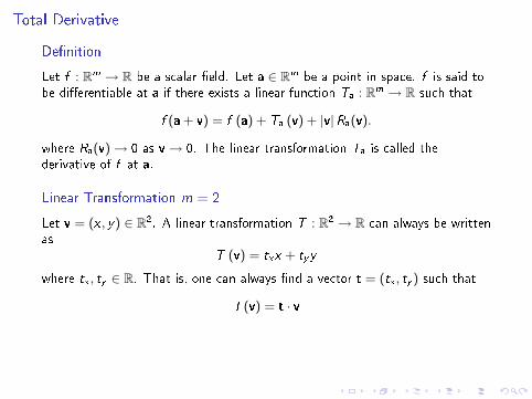
Linear Transformation m = 2
Let v = (x , y) ∈ R2. A linear transformation T : R2 → R can always be writtenas
T (v) = txx + tyy
where tx , ty ∈ R. That is, one can always �nd a vector t = (tx , ty ) such that
T (v) = t · v

Total Derivative
De�nition
Let f : Rm → R be a scalar �eld. Let a ∈ Rm be a point in space. f is said tobe di�erentiable at a if there exists a linear function Ta : Rm → R such that
f (a + v) = f (a) + Ta (v) + |v|Ra(v).
where Ra(v)→ 0 as v→ 0. The linear transformation Ta is called thederivative of f at a.
Linear Transformation
Let v ∈ Rm. A linear transformation T : Rm → R can always be written as
T (v) = t · v
where t ∈ Rm is some constant vector.

Total Derivative
De�nition
Let f : Rm → R be a scalar �eld. Let a ∈ Rm be a point in space. f is said tobe di�erentiable at a if there exists a linear function Ta : Rm → R such that
f (a + v) = f (a) + Ta (v) + |v|Ra(v).
where Ra(v)→ 0 as v→ 0. The linear transformation Ta is called thederivative of f at a.
Example
f (x , y) = x2 + y2, a = (1, 0), v = (x , y). Then
f (a + v) = f (x + 1, y) = (x + 1)2 + y2 = 1 + 2x + 0y + x2 + y2
= 1 + (2, 0) · v + |v|2
Thus Ta (v) = (2, 0) · v. And remember ∂∂x
f (a) = 2, ∂∂y
f (a) = 0.

Gradient
De�nition
Let f : Rm → R be a scalar �eld. Let a ∈ Rm be a point in space. f is said tobe di�erentiable at a if there exists a linear function Ta : Rm → R such that
f (a + v) = f (a) + Ta (v) + |v|Ra(v).
where Ra(v)→ 0 as v→ 0. The linear transformation Ta is called thederivative of f at a.
Let Ta = t · v where t ∈ Rm , the vector t is called thegradient of f at a and isdenoted by ∇f (a).

Properties of Gradient
Theorem
If f : R3 → R is a di�erentiable at a with total derivative Ta, then all partial
derivatives exist and
Ta (v) =
(∂
∂xf (a),
∂
∂yf (a),
∂
∂zf (a)
)· v
that is
∇f (a) =
(∂
∂xf (a),
∂
∂yf (a),
∂
∂zf (a)
).
Example
f (x , y) = x2 + y2, a = (1, 0), v = (x , y). Then Ta (v) = (2, 0) · v. And∂∂x
f (a) = 2, ∂∂y
f (a) = 0.
The converse of the previous theorem does hold.
Example
f (x , y) = xy2
x2+y2. Show that all partial derivatives of f exist at (0, 0) but total
derivative does not exist.

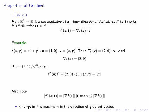
Properties of Gradient
Theorem
If f : R3 → R is a di�erentiable at a , then directional derivatives f ′ (a; t) exist
in all directions t and
f ′ (a; t) = ∇f (a) · t
Example
f (x , y) = x2 + y2, a = (1, 0), v = (x , y). Then Ta (v) = (2, 0) · v. And
∇f (a) = (2, 0)
If t = (1, 1) /√2, then
f ′ (a; t) = (2, 0) · (1, 1)/√2 =√2
Also note: ∣∣f ′ (a; t)∣∣ = |∇f (a)| |t| cosα ≤ |∇f (a)|I Change in f is maximum in the direction of gradient vector.

Properties of Gradient
Geometric Interpretation
Gradient Vector is always perpendicular to level curves and level surfaces.
-1.5 -1 -0.5 0 0.5 1 1.5-1.5
-1
-0.5
0
0.5
1
1.5
t
agradHfL
Along the tangent direction to alevel curve, directional derivativemust be 0! Function value does notchange in that direction. But then
f ′ (a; t) = ∇f (a) · t = 0

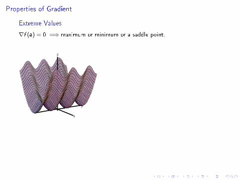
Properties of Gradient
Extreme Values
∇f (a) = 0 =⇒ maximum or minimum or a saddle point.
x
y
z
-4 -2 0 2 4
-7.5
-5
-2.5
0
2.5
5
7.5
Properties of Gradient
Extreme Values
∇f (a) = 0 =⇒ maximum or minimum or a saddle point.
x
y
z
-4 -2 0 2 4
-7.5
-5
-2.5
0
2.5
5
7.5

Properties of Gradient
Extreme Values
∇f (a) = 0 =⇒ maximum or minimum or a saddle point.
x
y
z
-4 -2 0 2 4
-7.5
-5
-2.5
0
2.5
5
7.5

Properties of Gradient
f and g are scalar �elds and c is a real constant
I ∇ (f + g) (a) = ∇f (a) +∇g(a)
I ∇ (cf ) = c∇fI ∇ (fg) = f∇g + g∇fI If r = (x , y , z) and r =
√x2 + y2 + z2, then ∇ (rn) = nrn−2r = nrn−1 r
I Chain Rule: f : R→ Rn and g : Rn → R and h = g ◦ f , thenh′(a) = ∇g · f ′(a)

Derivative of Vector Fields
De�nition
Let F : Rm → Rn be a vector �eld. Let a ∈ Rm be a point in space. F is said tobe di�erentiable at a if there exists a linear function Ta : Rm → Rn such that
F(a + v) = F (a) + Ta (v) + |v|Ra(v).
where Ra(v)→ 0 as v→ 0. The linear transformation Ta is called thederivative of f at a.
Linear Transformation m = n = 2
Let v = (x , y) ∈ R2. A linear transformation T : R2 → R2 can always bewritten as
T (v) =
[t11x + t12y
t21x + t22y
]=
[t11 t12t21 t22
] [x
y
]where t11, t12, t21, t22 ∈ R. That is, one can always �nd a matrix
t =
[t11 t12t21 t22
]such that
T (v) = t · v

Derivative of Vector Fields
De�nition
Let F : Rm → Rn be a vector �eld. Let a ∈ Rm be a point in space. F is said tobe di�erentiable at a if there exists a linear function Ta : Rm → Rn such that
F(a + v) = F (a) + Ta (v) + |v|Ra(v).
where Ra(v)→ 0 as v→ 0. The linear transformation Ta is called thederivative of f at a.
If F : R2 → R2 and F(a) =
[Fx(a)Fy (a)
]then
Ta(v) =
[∂Fx∂x
∂Fx∂y
∂Fy∂x
∂Fy∂y
] [x
y
]

Derivative of Vector Fields
De�nition
Let F : Rm → Rn be a vector �eld. Let a ∈ Rm be a point in space. F is said tobe di�erentiable at a if there exists a linear function Ta : Rm → Rn such that
F(a + v) = F (a) + Ta (v) + |v|Ra(v).
where Ra(v)→ 0 as v→ 0. The linear transformation Ta is called thederivative of f at a.
If F : R3 → R3 and F(a) =
Fx(a)Fy (a)Fz(a)
and v = (x , y , z) then
Ta(v) =
∂Fx∂x
∂Fx∂y
∂Fx∂z
∂Fy∂x
∂Fy∂y
∂Fy∂z
∂Fz∂x
∂Fz∂y
∂Fz∂z
x
y
z

Divergence and Curl of Vector Fields
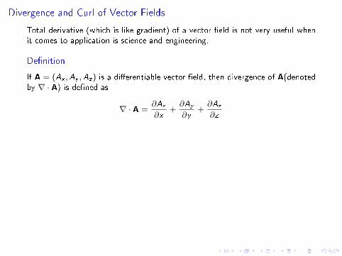
Total derivative (which is like gradient) of a vector �eld is not very useful whenit comes to application is science and engineering.
De�nition
If A = (Ax ,Ay ,Az) is a di�erentiable vector �eld, then divergence of A(denotedby ∇ · A) is de�ned as
∇ · A =∂Ax
∂x+∂Ay
∂y+∂Az
∂z
De�nition
If A = (Ax ,Ay ,Az) is a di�erentiable vector �eld, then curl of A(denoted by∇× A) is de�ned as
∇× A = x
(∂Az
∂y− ∂Ay
∂z
)+ y
(∂Ax
∂z− ∂Az
∂x
)+ z
(∂Ay
∂x− ∂Ax
∂y
)
Divergence and Curl of Vector Fields
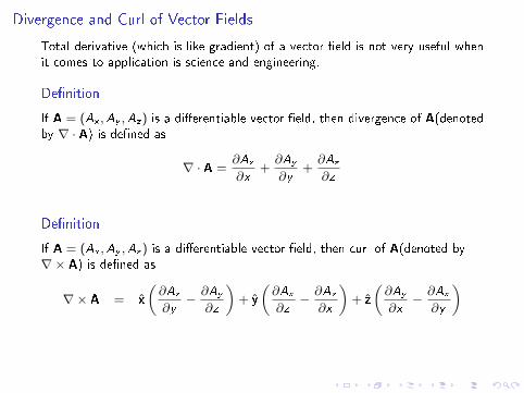
Total derivative (which is like gradient) of a vector �eld is not very useful whenit comes to application is science and engineering.
De�nition
If A = (Ax ,Ay ,Az) is a di�erentiable vector �eld, then divergence of A(denotedby ∇ · A) is de�ned as
∇ · A =∂Ax
∂x+∂Ay
∂y+∂Az
∂z
De�nition
If A = (Ax ,Ay ,Az) is a di�erentiable vector �eld, then curl of A(denoted by∇× A) is de�ned as
∇× A = x
(∂Az
∂y− ∂Ay
∂z
)+ y
(∂Ax
∂z− ∂Az
∂x
)+ z
(∂Ay
∂x− ∂Ax
∂y
)
Divergence and Curl of Vector Fields
Total derivative (which is like gradient) of a vector �eld is not very useful whenit comes to application is science and engineering.
De�nition
If A = (Ax ,Ay ,Az) is a di�erentiable vector �eld, then divergence of A(denotedby ∇ · A) is de�ned as
∇ · A =∂Ax
∂x+∂Ay
∂y+∂Az
∂z
De�nition
If A = (Ax ,Ay ,Az) is a di�erentiable vector �eld, then curl of A(denoted by∇× A) is de�ned as
∇× A = x
(∂Az
∂y− ∂Ay
∂z
)+ y
(∂Ax
∂z− ∂Az
∂x
)+ z
(∂Ay
∂x− ∂Ax
∂y
)

Gradient as an operator
It is useful to treat the symbol ∇ as a vector operator, that is when it operateson a scalar �eld and produces a vector �eld. It is conveniently written as
∇ = x∂
∂x+ y
∂
∂y+ z
∂
∂z


