Electromechanical Systems 1 - polito.it · Electromechanical Systems 1 Basilio Bona ... em as the...

Electromechanical Systems 1

Basilio Bona

DAUIN – Politecnico di Torino

Semester 1, 2015-16

B. Bona (DAUIN) Electromechanical Systems 1 Semester 1, 2015-16 1 / 39

Introduction

In a system that includes interacting mechanical and electromagneticcomponents, or that has an intrinsic electromechanical behaviour, aspiezoelectric, electro-rheological, and magnetostrictive materials, magneticshape memory alloys, and others, it is possible to define anelectromechanical Lagrangian function Lem as the sum of the Lagrangianfunctions related to the different components.

The Lagrangian function of the electromagnetic part of the system may bedefined using either the charge or the flux approach.

We the index ‘e’ to indicate the electromagnetic quantities, and the index‘m’ to indicate the mechanical quantities.


Generalized charge coordinates

In this approach we choose the electrical charges qe as the generalizedcoordinates for electromagnetical subsystems, and the linear/angulardisplacements qm as the generalized coordinates for mechanicalsubsystems.

Global generalized coordinates, global generalized velocities, and globalgeneralized forces are therefore

q =

[qmqe

]

, q =

[qmqe

]

, F =

[Fm

Fe

]

The total kinetic co-energy is the sum

K∗

em(q, q) = K∗

m(qm, qm) +W ∗

i (qe ,qm)

and the total potential energy is the sum

Pem(q) = Pm(qm) +Wc(qe ,qm)

Observe that the kinetic co-energy and the potential energy of theelectrical subsystem are influenced by the mechanical coordinates.


The total Lagrange function is

Lem(q, q) = K∗

em(q, q)− Pem(q)

= K∗

m(qm, qm)− Pm(qm) +W ∗

i (qe ,qm)−Wc(qe ,qm)

and the Lagrange equations are

d

dt

(∂Lem

∂qm

)

−∂Lem

∂qm= Fm i = 1, . . . , nm

d

dt

(∂Lem

∂qe

)

−∂Lem

∂qe= Fe i = 1, . . . , ne


Mechanical equations

d

dt

(∂K∗

m(qm, qm)

∂qm

)T

−

(∂K∗

m(qm, qm)

∂qm

)T

−

(∂W ∗

i (qe ,qm)

∂qm

)T

+

(∂Pm(qm)

∂qm

)T

+

(∂Wc (qe ,qm)

∂qm

)T

= Fm

Electrical equations

d

dt

(∂W ∗

i (qe ,qm)

∂qe

)T

+

(∂Wc(qe ,qm)

∂qe

)T

= Fe

where∂W ∗

i (qe ,qm)

∂qmand

∂Wc(qe ,qm)

∂qm

are respectively the change of magnetic/inductive kinetic co-energy due toa change in the mechanical coordinates, and the change of capacitivepotential energy due to a change in the mechanical coordinates.


Generalized flux coordinates

In this approach we choose the magnetic flux linkages λ as the generalizedcoordinates for electromagnetical subsystems, and the linear/angulardisplacements qm as the generalized coordinates for mechanicalsubsystems.

Global generalized coordinates, global generalized velocities, and globalgeneralized forces are

q =

[qmλ

]

, q =

[qmλ

]

, F =

[Fm

Fe

]

The total kinetic co-energy is the sum

K∗

em(q, q) = K∗

m(qm, qm) +W ∗

c (λ,qm)

and the total potential energy is the sum

Pem(q) = Pm(qm) +Wi (λ,qm)

Observe that the kinetic co-energy and the potential energy of theelectrical subsystem are influenced by the mechanical coordinates.


The total Lagrange function is

Lem(q, q) = K∗

em(q, q)−Pem(q)

= K∗

m(qm, qm)− Pm(qm) +W ∗

c (λ,qm)−Wi(λ,qm)

and the Lagrange equations are

d

dt

(∂Lem

∂qm

)

−∂Lem

∂qm= Fm i = 1, . . . , nm

d

dt

(∂Lem

∂λ

)

−∂Lem

∂λ= Fe i = 1, . . . , ne


Mechanical equations

d

dt

(∂K∗

m(qm, qm)

∂qm

)T

−

(∂K∗

m(qm, qm)

∂qm

)T

−

(

∂W ∗

c (λ,qm)

∂qm

)T

+

(∂Pm(qm)

∂qm

)T

+

(∂Wi (λ,qm)

∂qm

)T

= Fm

Electrical equations

d

dt

(

∂W ∗

c (λ,qm)

∂λ

)T

+

(∂Wi(λ,qm)

∂λ

)T

= F e

where∂W ∗

c (λ,qm)

∂qmand

∂Wi (λ,qm)

∂qm

are respectively the change of magnetic/inductive kinetic co-energy due toa change in the mechanical coordinates, and the change of capacitivepotential energy due to a change in the mechanical coordinates.


Electromechanical Two-port Networks

We consider a particular class of electromechanical systems, the two-portnetworks, whose inner structure may be represented by characteristicsthat can be either mainly inductive or mainly capacitive.

An electrical two-port network is a network that presents two ports; one isthe input port the other is the output port.

When the ports can be reversed, i.e., the input becomes the output andvice-versa, the network is called a reversible two-port network.

If inside the network no electrical power sources are present, the two-portis called passive two-port network, otherwise it is an active two-portnetwork.

The physical quantities at the two ports are always a quantity called efforts(t) and a quantity called flux φ(t).

The effort-flux couples (s(t), φ(t)) may be electrical or mechanical at bothports, or different at the two ports; we consider this last class of two-portsystems.


The electrical port is characterized by a voltage s(t) = e(t) and a currentφ(t) = i(t), while the mechanical port is characterized by a forces(t) = f (t) and a velocity φ(t) = v(t).

The port power is the product P(t) = s(t)φ(t). Figure shows a two-portsystems, where the input port is located on the left side and the outputport on the right side. Pi(t) is the inflowing input power, Po(t) is theoutflowing output power.


Inductive two-port networks

In this type of two-port network the power conversion is obtained by aninductive element characterized by a flux linkage λ(t).


The two-port system is characterized by the following constitutive relations

i(t) = i(λ(t), x(t))

f (t) = f (λ(t), x(t))

and

e(t) =dλ(t)

dt= λ(t)

v(t) =dx(t)

dt= x(t)

where x(t) represents a displacement.

These relations are generic; they must be specified according to the typeof electromagnetic interactions of the considered system.


The power absorbed by the system is given by the difference between theinput and the output power

Pλ(t) = Pi (t)− Po(t) = e(t)i(t)− f (t)v(t) = λ(t)i(t)− f (t)x(t)

Considering the energy, we can write

Pλdt = dWi(λ, x) = i dλ− f dx

and, since

dWi (λ, x) =∂Wi (λ, x)

∂λdλ+

∂Wi (λ, x)

∂xdx ,

comparing the above relations one obtains

i(λ, x) =∂Wi (λ, x)

∂λand f (λ, x) = −

∂Wi(λ, x)

∂x


Considering the co-energy, we can write

W ∗

i (i , x) = λi −Wi(λ, x)

and taking the differential work, we have

dW ∗

i (i , x) = i dλ+ λdi − dWi (λ, x)

Since we can writei dλ− dWi(λ, x) = f dx

we obtaindW ∗

i (i , x) = λdi + f dx

Recalling that

dW ∗

i (i , x) =∂W ∗

i (i , x)

∂idi +

∂W ∗

i (i , x)

∂xdx

it follows that

λ(i , x) =∂W ∗

i (i , x)

∂i; f (i , x) =

∂W ∗

i (i , x)

∂x


We can summarize the above relations as follows

dWi(λ, x) = i dλ− f dx dW ∗


i(λ, x) =∂Wi (λ, x)

∂λλ(i , x) =

∂W ∗

i (i , x)

∂i

f (λ, x) = −∂Wi(λ, x)

∂xf (i , x) =

∂W ∗

i (i , x)

∂x

The constitutive relations are now defined as the partial derivatives of theenergy; the flux linkage is the partial derivative of the co-energy, and theforce f can be expressed as a function of λ(t) or i(t).


Linear flux

Let us assume that the flux is linear with respect to the current i(t)

λ(i , x) = L(x)i(t)

where L(x) represents the magnetic circuit inductance, in general functionof a mechanical displacement x(t). We can write

W ∗

i (i , x) =1

2L(x)i2(t)

and

f (λ, x) =1

2

λ2

L2(x)

d

dxL(x)

or

f (i , x) =1

2i2

d

dxL(x)


The voltage e(t) is given by

e(t) =d

dt[L(x)i ] = L(x)

di

dt+ i

∂L(x)

∂xx

or

e = L(x)di

dt+ e′

where the voltage

e′ = i∂L(x)

∂xx

is due to the variation of the auto-inductance when the circuit is subject toa mechanical deformation.


Capacitive two-port networks

In this type of two-port network the power conversion is obtained by acapacitive element characterized by an electrical charge q(t).


The two-port system is characterized by the following constitutive relations

e(t) = e(q(t), x(t))

f (t) = f (q(t), x(t))

and

i(t) =dq(t)

dt= q(t)

v(t) =dx(t)

dt= x(t)

where x(t) represents a displacement.

These relations are generic; they must be specified according to the typeof electromagnetic interactions of the considered system.


The power absorbed by the system is given by the difference between theinput and the output power

Pq(t) = Pi (t)− Po(t) = e(t)i(t)− f (t)v(t) = e(t)q(t)− f (t)x(t)

Considering the energy, we can write

Pq dt = dWc(q, x) = e dq − f dx

and, since

dWc(q, x) =∂Wc(q, x)

∂qdq +

∂Wc(q, x)

∂xdx ,

comparing the above relations to one obtains

e(q, x) =∂Wc(q, x)

∂qand f (q, x) = −

∂Wc(q, x)

∂x


considering the co-energy, we can write

W ∗

c (e, x) = eq −Wc(q, x)

and, considering the virtual work, we have

dW ∗

c (e, x) = e dq + q de − dWc(q, x)

Since we can writee dq − dWc(q, x) = f dx

we have at the enddW ∗

c (e, x) = q de + f dx

Recalling that, in general

dW ∗

c (e, x) =∂W ∗

c (e, x)

∂ede +

∂W ∗

c (e, x)

∂xdx

it follows immediately that

q(e, x) =∂W ∗

c (e, x)

∂e; f (e, x) =

∂W ∗

c (e, x)

∂x


We can summarize the above relations as follows

dWc(q, x) = edq − f dx dW ∗

c (e, x) = qde + f dx

e(q, x) =∂Wc(q, x)

∂qq(e, x) =

∂W ∗

c (e, x)

∂e

f (q, x) = −∂Wc(q, x)

∂xf (e, x) =

∂W ∗

c (e, x)

∂x

The constitutive relations are now defined as the partial derivatives of theenergy; the charge is the partial derivative of the co-energy, and the forcef can be expressed as a function of q(t) or e(t).


Linear charge

Let us assume that the charge is linear with respect to the voltage e(t)

q(e, x) = C (x)e(t)

where C (x) represents the capacity related to the electrostaticphenomenon, in general function of a mechanical displacement x(t). Wecan write

Wc(q, x) =1

2

q2(t)

C (x)

and

f (q, x) = −q2

2

d

dx

[1

C (x)

]

or f (e, x) =e2

2

d

dxC (x)


The current i(t) is given by

i(t) =d

dt[C (x)e ] = C (x)

de

dt+ e

∂C (x)

∂xx

or

i = C (x)de

dt+ i ′

where the current

i ′ = e∂C (x)

∂xx

is due to the capacity variation when the circuit is subject to a mechanicaldeformation.


Example – Magnetic suspension


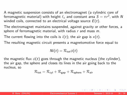
A magnetic suspension consists of an electromagnet (a cylindric core offerromagnetic material) with height ℓc and constant area S = πr2, with Nwinded coils, connected to an electrical voltage source E (t).

The electromagnet maintains suspended, against gravity or other forces, asphere of ferromagnetic material, with radius r and mass m.

The current flowing into the coils is i(t); the air gap is x(t).

The resulting magnetic circuit presents a magnetomotive force equal to

Ni(t) = Rtotφ(t)

the magnetic flux φ(t) goes through the magnetic nucleus (the cylinder),the air gap, the sphere and closes its lines in the air going back to thenucleus, so

Rtot = Rcyl +Rgap +Rsphere +Rair


the circuit is made of ferromagnetic material with µ ≫ µ0, the tworeluctances Rcyl and Rsphere are negligible with respect to Rgap and Rair

If the sphere is sufficiently near to the nucleus, the length of the remainingpath through air back to the nucleus is approximately constant withrespect to the sphere motion.

SinceRgap =

x

µ0S

where µ0 is the air permeability, one can write

Rgap +Rair =x + ℓ0

µ0S

where ℓ0 = Rairµ0S is the equivalent length of the flux in air.


It follows that

Ni(t) =x + ℓ0

µ0Sφ(t)

and then

λ = Nφ(t) =N2µ0S

ℓ0 + xi(t)

In conclusion, the circuit inductance is

L(x) =N2µ0S

ℓ0 + x=

kL

ℓ0 + x

with kL = N2µ0S .

The electrical circuit is powered by an ideal voltage generator E (t) inseries with a resistance R , and a negligible capacitance; the dynamicalequations of the magnetic suspension can be computed assuming asgeneralized coordinates the electrical charge q(t) and the mechanicaldisplacement x(t) of the sphere.


Applying the charge approach for the electrical part, where no capacitiveelements are present, we have

K∗

m =1

2mx2

K∗

e = W ∗

i (q, x) =1

2L(x)q2

Pm = −mGx

Pe = Wc(q) =1

2

q2

C= 0

Dm =1

2βx2 ≈ 0 if β ≈ 0

De =1

2Rq2

Fm = 0

Fe = E (t)

where G is the gravity acceleration value and the viscous friction isnegligible.


Lagrange Equation 1)

d

dt

∂K∗

m

∂x−

∂(K∗

e − Pm)

∂x+

∂Dm

∂x= 0

whenced

dtmx +

k

2(ℓ0 + x)2q2 −mG + βx = 0

and, neglecting the friction force,

mx = mG −k

2(ℓ0 + x)2q2

or

mx(t) = mG −k

2(ℓ0 + x(t))2i2(t)



d

dt

∂K∗

e

∂q+

∂De

∂q= E (t)

whenced

dt[L(x)q ] + Rq = E (t)

therefored

dt[L(x) ] q + L(x)

d

dt[q ] + Rq = E (t)

and

−k

(ℓ0 + x)2x q + L(x)q + Rq = E (t)

that can also be written as

L(x)d

dti(t) + Ri(t) = E (t) +

kx(t)

(ℓ0 + x(t))2i(t)


Example – Voice coil


A voice coil consists of a fixed magnetic circuit, composed by a permanentmagnet suitably inserted into a ferromagnetic circuit. A mobile elementwith several coils (moving coils), interacts with the magnetic circuit and isfree to move along one direction.

The interaction between the permanent magnet circuit field and theelectromagnetic field generated by the current in the coils, causes themotion of the moving coil.

During its motion, the number of coils that “cut” the magnetic flux linesvaries in function of the coils displacement x .

The mechanical part is characterized by the mass m of the moving coiland attachments, by the friction coefficient β that models the dissipativeeffects due to the air motion, and by the elastic coefficient k that modelsthe elastic effect of the membrane suspensions.

The electrical part of the actuator is characterized by a fixedauto-inductance L due to the coils, by a resistance R and by a variablevoltage source E (t); the capacitive effects are negligible.


The permanent magnet generates a magnetic field whose closed flux linesdivide into the superior and inferior part of the magnetic circuit; the fielddensity B is constant in the air gap. The magnetic flux Φm that interactsthe electrical windings depends on the surface interested by thephenomenon, that is

Φm = 2πrx ‖B‖

where we have indicate with x the position of the coil with respect to theexternal surface of the magnetic circuit. The flux linked to the coilsdepends on two terms: the first one, Φa, is due to the auto-induced fluxproduced by the current that transverses the coil, the second one, Φm, isthat produced by the permanent magnet and linked with the “active” coils:

λ(i , x) = Φa + Φm = Li + Kex (1)

where L is the auto-inductance of the coil with N windings andKe = 2πrN ‖B‖.


Applying the charge approach for the electrical part, where no capacitiveelements are present, we have

K∗

m =1

2mx2

K∗

e = W ∗

i (q, x)

Pm =1

2kx2

Pe = Wc(q) =1

2

q2

C= 0

Dm =1

2βx2

De =1

2Rq2

Fm = 0

Fe = E (t)


In this case the term K∗

e = W ∗

i (i , x) is more complex. We recall that

dW ∗


hence

W ∗

i (i , x) =

∫∫

i ,x

dW ∗

i (i , x) =

∫∫

i ,x

λdi ′ + f dx ′

where x ′ and i ′ are the generic integration variables. If in the plane (i , x)we chose as integration path from (0, 0) to (0, x), and then from (0, x) to(i , x), we can express the previous integral as

W ∗

i (i , x) =

∫ x

0f (i = 0, x ′)dx ′ +

∫ i

0λ(i ′, x)di ′

Since it is reasonable to assume that when the flux linkage is zero, theforce is also zero, i.e., f (i = 0, x ′) = 0 for any value of x , we have

W ∗

i (i , x) =

∫ x

0f (0, x ′)dx ′

︸︷︷︸

=0

+

∫ i

0λ(i ′, x)di ′ =

∫ i

0(Li ′+Kex)di

′ =1

2Li2+Kexi



d

dt

∂K∗

m

∂x−

∂(K∗

e − Pm)

∂x+

∂Dm

∂x= 0

givesd

dtmx + kx − Ke q + βx = 0

and, considering the friction force,one obtains

mx + βx + kx = Ke q

ormx(t) + βx(t) + kx(t) = Ke i(t)



d

dt

∂K∗

e

∂q+

∂De

∂q= E (t)

givesd

dt[Lq + Kex ] + Rq = E (t)

orLq + Ke x + Rq = E (t)

that we can write as

Ld

dti(t) + Ri(t) = E (t)− Ke x(t)


Notice the term appearing in Equation 1), namely

Ke i(t)

When a two-port network contains an inductive element and the fluxlinkage is linear in the current, one can write

f (i , x) =∂W ∗

m(i , x)

∂x

that in our case becomesf (i , x) = Ke i .

Similarly, in Equation 2) there is the term Ke x , that can be associated tothe voltage

e(t) = λ(t) =d

dt[Li + Kex ] = L

di

dt+ e′(t)

with e′(t) = Ke x(t)


Date post:	24-Jan-2019
Category:	Documents
Upload:	lamdung
View:	223 times
Download:	1 times

Electromechanical Systems 1 - polito.it · Electromechanical Systems 1 Basilio Bona ... em as the...

Documents