72
Electron-phonon coupling in
graphene
Bo Hellsing, Department of Physics, Gothenburg, Sweden
January , 2019

Outline
1. Electron-Phonon coupling
2. Lifetime broadening - Theory
3. Electrons in graphene
4. Phonons in graphene
5. Lifetime broadening of Graphene bands
6. Master thesis projects
http://fy.chalmers.se/∼hellsing/student_projects/EPC_seminars_2019.2.pdf

1. Electron-Phonon coupling
Electron-Phonon Coupling (EPC)
I Fundamental interest
I Damping of vibrational excitations and electronic friction
I Lifetime of electronic excitations
I Photoinduced surface reactions
I Superconductivity(BCS theory: I. Eremin, Max-Planck Institut
[https://www.pks.mpg.de/ ieremin/teaching/wroclaw1.pdf])

Fundamentals
Many important chemical and physical phenomena are inuenced byinherent dissipative processes which involve energy transfer betweenthe electrons (electron-electron scattering) and between theelectrons and the ionic motion (electron-phonon scattering) - EPC.
Non-adiabatic interaction between the valence electrons and the ionmotion in a solid reveals the break down of the Born-Oppenheimerapproximation Electrons are not innitely fast !
ωplasmonωphonon
≈ 103

Electron-phonon coupling inuences e.g vibrational damping ofadsorbates and lifetime of excited surface states.
Several experimental techniques, e.g. HREELS, IR and ARPES areable to give information about the importance of EPC
Combined with advanced theoretical calculations it is possible tosort out the relative importance of EPC and to point out keyparameters.
Graphene has recently surprised us with a strong electron-phononcoupling. Utilizing this property to modify graphene to become asuperconductor is a challenge.
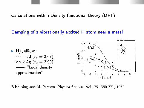
Calculations within Density functional theory (DFT)
Damping of a vibrationally excited H atom near a metal
I H/Jellium:· · · · · Al (rs = 2.07)x x x Ag (rs = 3.00)- Local densityapproximation
B.Hellsing and M. Persson, Physica Scripta. Vol. 29. 360-371, 1984

Electronic friction at surfaces
I The friction coecient in terms of the stochastic force
η =1
kBRe
∫ ∞0
dt < F st(t)Fst(0) > =M
~Γ
A thermal H atom approaching a Jellium surface
B.Hellsing and M. Persson, Physica Scripta. Vol. 29. 360-371, 1984
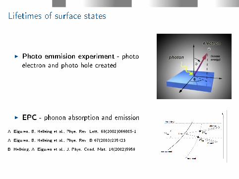
Lifetimes of surface states
I Photo emmision experiment - photoelectron and photo hole created
I EPC - phonon absorption and emission
A. Eiguren, B. Hellsing et al., Phys. Rev. Lett. 88(2002)066805-1
A. Eiguren, B. Hellsing et al., Phys. Rev. B 67(2003)235423
B. Hellsing, A. Eiguren et al., J. Phys. Cond. Mat. 14(2002)5959

Experiment and Calculations
Cu(111) and Ag(111):
I T = 0 : (⇒ nB = 0)
Γnk = 2π
∫ ωmax
0α2Fki(ω)dω
I high T : kBT >> ~ωmax
Γnk(T ) = 2πλnkkBT
A. Eiguren, B. Hellsing, F. Reinert et al.,
Phys. Rev. Lett. 88(2002)066805-1

Mini many-body course
The Greens' function related to a state |a〉 is written
Ga(ε) =1
ε− εa − iδWith this construction of the Greens' function the imaginary partwill give the spectrum
1
πImGa(ε) =
1
π
δ
(ε− εa)2 + δ2= δ(ε− εa)
Now if we consider this pure state coupled to some other degrees offreedom, e.g. phonons we replace the iδ in the denominator of theGreens' function of the pure state |a〉 by a complex so calledself-energy Σa(ε).

Ga(ε) =1
ε− εa − Σa(ε)
where
Σa(ε) = ReΣa(ε) + iImΣa(ε)
Taking again the imaginary part of the Greens' function we get thespectrum or what is also called the Spectral function Aa(ε).
Aa(ε) =1
πImGa
In the band picture we label the states with n and k and we get
An(ε,k) =1
π
ImΣn(ε,k)
(ε− εn(k)−ReΣn(ε,k))2 + (ImΣn(ε,k))2
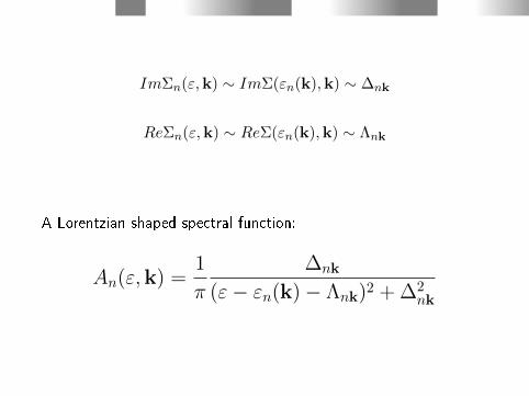
ImΣn(ε,k) ∼ ImΣ(εn(k),k) ∼ ∆nk
ReΣn(ε,k) ∼ ReΣ(εn(k),k) ∼ Λnk
A Lorentzian shaped spectral function:
An(ε,k) =1
π
∆nk
(ε− εn(k)− Λnk)2 + ∆2nk

Spectral function - Photo Emission Spectroscopy (EPS)
In the sudden approximation the spectral function An(ε,k)corresponds to the photoemission peak.
Line width = Lifetime broadening (FWHM): Γnk = 2∆nk
We sum up all phonon induced electron scattering processes fromoccupied states to the photo-hole (nk), requiring momentum andenergy conservation. The temperature is below any characteristicphonon energy ⇒ only phonon emission takes plays.

Γnk from ARPES
ARPES = Angular Resolved PhotoEmission Spectroscopy
Lindwidth Γnk ↔ Hole lifetime τnk
Heisenberg : ∆E∆t ≥ ~ ⇒ τnk ≥~
Γnk
Intra-band scattering Inter-band scattering
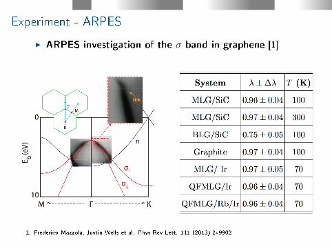
Experiment - ARPES
I ARPES investigation of the σ band in graphene [1]
1. Frederico Mazzola, Justin Wells et al. Phys Rev Lett. 111 (2013) 249902
2. Lifetime broadening
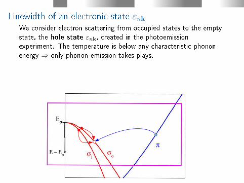
Linewidth of an electronic state εnkWe consider electron scattering from occupied states to the emptystate, the hole state εnk, created in the photoemissionexperiment. The temperature is below any characteristic phononenergy ⇒ only phonon emission takes plays.

Electron scattering with phonon emission can take place fromelectron states n′k′ to the photo hole state nk.Momentum conservation:
k = k′ + q±G
q is a phonon wave vector, G is a reciprocal lattice vector.Energy conservation (phonon emission):
εnk = εn′k′ − ~ωνq
~ωνq is a phonon energy of mode ν and momentum q.
According to the Heisenberg uncertainty relation the decay ratetimes ~ gives the so called lifetime broadening or linewidth.
We are aiming the EPC contribution to the width of the peak(linewidth) of the spectral function recorded in the photoemissionexperiment.
Applying rst order time dependent perturbation theory - GoldenRule - the lifetime broadening can be calculated.

Perturbation theoryPerturbation theory: Q = ion displacement and x = electroncoordinate :
H(Q, x) ≈ H(0, x) +δH
δQQ = H(0, x) +
δV
δQQ
V is the one-electron potential. In the harmonic approximation
〈I = 1, n|H(Q, x)|I = 0,m〉 = 〈1|Q|0〉〈n|δVδQ|m〉 =√
~2MΩ
〈n|δVδQ|m〉, (1)
εm = εn + ~Ω

Fermi Golden Rule
Γnk = 2π∑n′νq
|〈nk|δV νq |n′k + q〉|2δ(εn′k+q − εnk − ~ωνq) (2)
δV = ∇ ~QV · ~Q , n is electronic band index, k electron wave vector,ν vibrational mode index and q the phonon wave vector.
The delta function takes care of the energy and momentumconservation.

In the harmonic approximation we have
δV νq (r) =√
~2Mων(q)
∑R[eν(q) · v′(R + rs; r)]e−iq·(R+rs) , (3)
R denotes location of unite cells, eν(q) is a Ns×3 dimensionalpolarization vector with components eνsi(q), where s labels theatoms in the unit cell (s =1,2,3 ,..,Ns, where Ns is the number ofatoms in the unite cell). Index i refers to the three cartesiancoordinates, x, y and z.
v′(R; r)
is the deformation potential with Ns×3 componentsv′si(R + rs; r) = ∂Vs
∂Qi(r− (R + rs)) where index i refers to the
displacement vector ( Qi = Qx, Qy, Qz ).

One-electron model potential
I chose a spherically symmetric smooth attractive Gaussian shapedeective one-electron potential with two parameters.
V (r) = V (r) = −V0e−(rα)2 (4)
V0 and α represents the strength (depth) and the real spaceextension (screening length), respectively.The phonon induced perturbation to rst order
δVν =∂V
∂QνQν ,
where Qν is the ionic displacement coordinate of the vibrationalmode ν.
Deformation potential
We apply the Rigid ion approximation (RIA). RIA corresponds to anapproximation when the electron potential is rigidly displaced withthe ionic displacement. This is a reasonable approximation if thescreening is sucient to yield a perturbation which is not felt byneighboring ions. We then have
V (Q, r) = V (r−Q)

If we for example consider an ionic displacement along thex-direction, the deformation potential is
δVx(r) =∂V
∂Qx·Qx = −∂V
∂x·Qx = x · 2V0
α2e−(
rα)2 ·Qx
In the harmonic approximation the squared magnitude of the meanionic displacement is
|〈0|Qν(q)|1〉|2 =~
2Mων(q)

Γ⇐⇒ λAt zero temperature (T=0) we have
Γnk = 2π~∫ ∞o
α2Fnk(ω)dω
and the local electron-phonon coupling constant λnk
λnk = 2
∫ ∞o
α2Fnk(ω)
ωdω
where α2Fnk(ω) is the Eliashberg function. This function can beseen as the phonon density of states weighted by theelectron-phonon coupling. The integration is over all phononfrequencies.
λ(ε) =∑nk
λnkδ(ε− εnk) , λ = λ(εF) (5)

3. Electrons in graphene

Electrons in graphene - a Tight Binding Model
In the tight-binding model the one-electron wave function is written
ψnk(r) =∑js
cnsj(k)Φsj(k, r) (6)
Bloch orbitals
Φsj(k, r) =1√N
∑R
φj(r− (R + rs))eik·(R+rs)
s = A,B denotes the two non-equivalent sites of the carbonatoms. R is a lattice vector connecting the unit cells. N is thenumber of unit cells we sum over. rA and rB are the position ofthe A and B atom relative the center of the unit cell.

The local atomic basis hydrogen-atom-like wave functions are
φj = φ2s, φ2px , φ2py , φ2pz
The radial part of the carbon atom basis according to Slater [Slateret al. Physical Review 36, 57 (1930)]
Rn = R2 ∼ re−Z∗r/2 , r =
√x2 + y2 + z2
where Z∗ = 3.25 a.u. is the screened eective charge seen by the2s and 2p electrons in carbon atom.

The normalized basis functions in cartesian coordinates are:
φ2s =(Z∗)5/2√
96πre−Z
∗r/2 , φ2pz =(Z∗)5/2√
32πze−Z
∗r/2
φ2px =(Z∗)5/2√
32πxe−Z
∗r/2 , φ2py =(Z∗)5/2√
32πye−Z
∗r/2
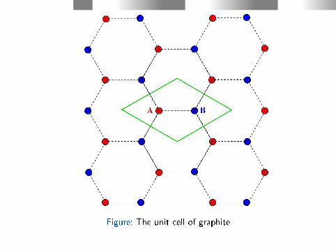
Figure: The unit cell of graphite

The generalized eigenvalue problem:
H ~ψ = εS ~ψ
where H and S is the Hamiltonian and overlap matrix
We have to diagonalize a (8X8) matrix to solve∑s′j′
〈sj|H − εS|s′j′〉cs′j′ = 0
(I do this using the LAPAK subroutine ZHEGV)
⇒ (εnk, cnsj(k))⇒ (εnk, ψnk)
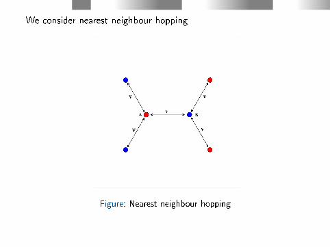
We consider nearest neighbour hopping
Figure: Nearest neighbour hopping

Details:
For a given electron momentum k:
〈sj|H − ε(k)S|s′j′〉 =
c∗sj(k)cs′j′(k)
∞∑l=1
〈φsj(r−Rs0)|H − ε(k)S|φs′j′(r− (Rs
l′ −Rs
0))〉×
eik ·(Rs′l −R
s0) ≈
(Nearest neighbour interaction: A has three B neighbours and B has
three A neighbours)
c∗sj(k)cs′j′(k)
3∑l=1
〈φsj(r−Rs0)|H − ε(k)S|φs′j′(r− (Rs
l′ −Rs
0))〉×
eik ·(Rsl′−Rs
0)
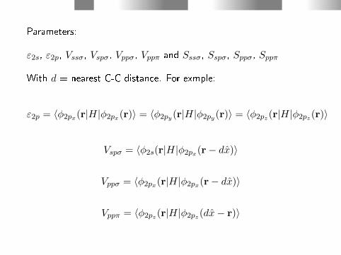
Parameters:
ε2s, ε2p, Vssσ, Vspσ, Vppσ, Vppπ and Sssσ, Sspσ, Sppσ, Sppπ
With d = nearest C-C distance. For exmple:
ε2p = 〈φ2px(r|H|φ2px(r)〉 = 〈φ2py(r|H|φ2py(r)〉 = 〈φ2pz(r|H|φ2pz(r)〉
Vspσ = 〈φ2s(r|H|φ2px(r− dx)〉
Vppσ = 〈φ2px(r|H|φ2px(r− dx)〉
Vppπ = 〈φ2pz(r|H|φ2pz(dx− r)〉
-20
-15
-10
-5
0
5
10
15
EF-E
(eV
)
i
o
M K
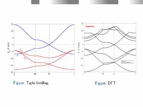
Figure: Tight-binding
M K
-15
-10
-5
0
5
10
15
E -
E_F
[eV
]
Graphene
pseudopot:
C.pbe-n-rrkjus-psl.1.0.0
Figure: DFT
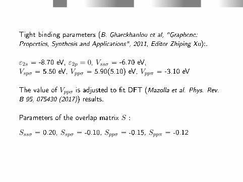
Tight binding parameters (B. Gharekhanlou et al, "Graphene:
Properties, Synthesis and Applications", 2011, Editor Zhiping Xu):.
ε2s = -8.70 eV, ε2p = 0, Vssσ = -6.70 eV,Vspσ = 5.50 eV, Vppσ = 5.90(5.10) eV, Vppπ = -3.10 eV
The value of Vppσ is adjusted to t DFT (Mazolla et al. Phys. Rev.
B 95, 075430 (2017)) results.
Parameters of the overlap matrix S :
Sssσ = 0.20, Sspσ = -0.10, Sppσ = -0.15, Sppπ = -0.12

4. Phonons in graphene

Phonons in graphene - a Force Constant Model
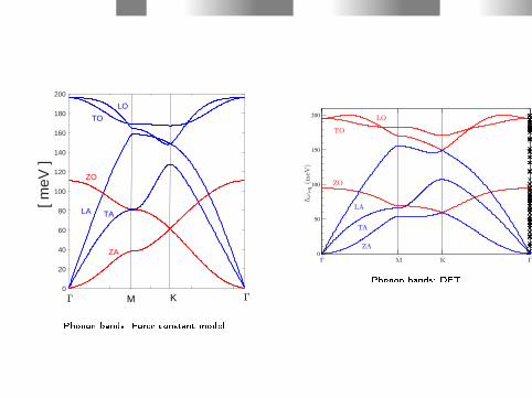
We consider all six phonon modes, three optical and three acoustic;
The optical phonon modes are: longitudinal optical (LO),transversal optical (TO) and out-of-plane optical (ZO).
The acoustic phonon modes are: longitudinal acoustic (LA),transversal acoustic (TA) and the out-of-plane acoustic(ZA).applying a constant force model.
Setting up the Dynamical matrix we include up to third ordernearest neighbor interactions. I apply the nine force constant modelby Falkovsky (L.A. Falkovsky, Phys.Lett. A 372, 5189 (2008)) and (B.Hellsing et al., Phys. Rev. B 98, 205428 (2018)).

Figure: Third order neighbour interaction

The dynamical matrix D is calculated including up to third ordernearest neighbor interactions. The force constants ΦAs
ll′ are denedby
DAsll′ (q) =
∑Rs
ΦAsll′ (Rs)e
−iq·Rs , (7)
Rs labels the vectors from a center A atom to the three nearest Batom, the six next-nearest A atoms and the three next-next-nearestB atoms.
l denotes the components of a complex vector (ξ, η).
ξ = X + iY and η = X − iY ,
X‖ = Xx+ Y y is the atomic in-plane displacement vector.
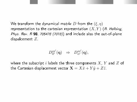
We transform the dynamical matrix D from the (ξ, η)representation to the cartesian representation (X,Y ) (B. Hellsing,Phys. Rev. B 98, 205428 (2018)) and include also the out-of-planedispalcement Z.
Dss′ll′ (q) ⇒ Dss′
ii′ (q),
where the subscript i labels the three components X, Y and Z ofthe Cartesian displacement vector X = Xx+ Y y + Zz.
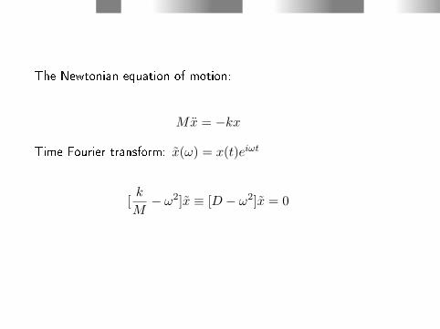
The Newtonian equation of motion:
Mx = −kx
Time Fourier transform: x(ω) = x(t)eiωt
[k
M− ω2]x ≡ [D − ω2]x = 0

The equation of motion give us an eigenvalue problem to solve:
∑s′i′
[Dss′ii′ (q)− ω2
ν(q)δss′δii′ ]eνs′i′(q) = 0 , (8)
The solutions give us the dispersion of the six eigen modes ων(q).eν is the 6-dimensional phonon polarization vector for eachvibrational.
0
20
40
60
80
100
120
140
160
180
200
[ meV
]
KM
ZO
TALA
TO
LO
ZA
Phonon bands: Force constant model
0
50
100
150
200
LA
TA
ZA
LO
TO
ZO
hωνq(m
eV)
ΓΓ M K
Phonon bands: DFT

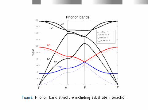
Interaction with the substrate
Figure: EELS Experiment [T. Aizawa et al., PRB 42, 469 (1990) ]

I introduce a spring between all the carbon atoms and a rigidsubstrate.
The spring constant is set to t the nite frequency of the ZAmodel at q=0. According to experiments [T. Aizawa, R. Souda, S.Otani, Y. Ishizawa, and C. Oshima, Phys. Rev. B 42, 469 (1990) ],~ωZA(q = 0) ≈ 35 meV for four dierent transition metal carbidesubstrates.

sks
k
B
B
A
B
k
k
k
k
A B
z
x
x
y
Figure: Graphene attached to a rigid substrate
0 0.2 0.4 0.6 0.8 1 1.2 1.4 1.6 1.8 20
20
40
60
80
100
120
140
160
180
200
meV
Phonon bands
KM
"ZA"
LO
TO
ZO
TALA
z=-1.45 cm -2
'z=0.085 cm -2
z=0.171 cm -2
sub=0.790 cm -2
Figure: Phonon band structure including substrate interaction

5. Lifetime broadening of Graphene bands

EPC matrix element
With the wave functions given in Eq. (6) we have that the EPCmatrix element is given by
〈nk|δV νq |n′k′〉 = 1N
∑sj
∑s′j′ c
∗nsjcn′s′j′
×∑
R,R′,R′′〈φj(x− (R+rs))δvνq(x− (R′′+r′′s ))φj′(x− (R′+rs′))〉u.c.
×e−ik·(R+rs)e−iq·(R′′+r′′s )eik
′·(R′+r′s) ,
where
δvνq(x) =
√~
2Mων(q)[eν(q) · v′(x)] , (9)
R is the lattice vectors connecting the centers of the unit cells and andrA and rB give the position of the A and B atoms relative the center ofthe unit cell.
N is the number of unit cells summed over and 〈.....〉u.c. denotesreal space integration over the unit cell.
In the numerical calculation I consider a cluster of 7 unit cells(N=7), one central and the 6 nearest.
The real-space integration is taken over the central unit cell. Thiscorresponds to R′′ = 0 and then we multiply with N . Thiseliminates N in the denominator in the previous equation.
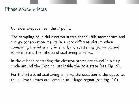
Phase space eects
Consider ~k-space near the Γ point.
The sampling of initial electron states that fullls momentum andenergy conservation results in a very dierent picture whencomparing the intra and inter σ band scattering (σo → σo andσi → σo) and the interband scattering π → σo.
In the σ band scattering the electron states are found in a tinycircle around the Γ-point just inside the hole state (see Fig. 9).
For the interband scattering π → σo the situation is the opposite,the electron states are sampled in a large region (see Fig. 10).
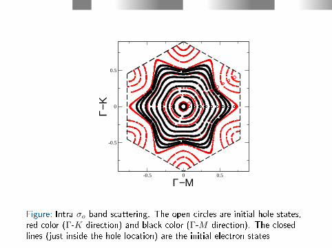
-0.5 0 0.5
Γ−Μ
-0.5
0
0.5
Γ−Κ
Figure: Intra σo band scattering. The open circles are initial hole states,red color (Γ-K direction) and black color (Γ-M direction). The closedlines (just inside the hole location) are the initial electron states
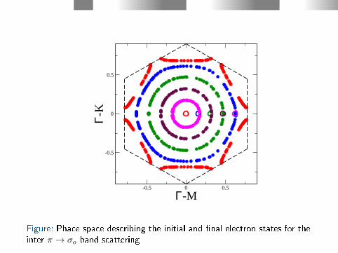
-0.5 0 0.5
Γ-M
-0.5
0
0.5
Γ-K
Figure: Phace space describing the initial and nal electron states for theinter π → σo band scattering

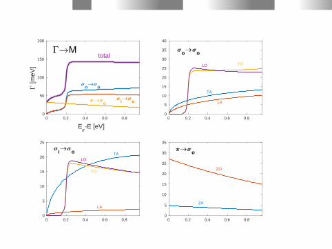
Linewidth Γ - ARPES experiments

Linewidth Γ - calculation
σo - band
18
16
14
12
10
8
6
4
2
0
EF-E
[ eV
]
i
o
KM

0 0.2 0.4 0.6 0.8 1
E -E [eV]
0
50
100
150
200
250
300
[meV
]
0 0.2 0.4 0.6 0.8 10
10
20
30
40
50
0 0.2 0.4 0.6 0.8 10
5
10
15
20
25
30
35
40
0 0.2 0.4 0.6 0.8 10
20
40
60
80
100
120
140
K
o o
i o
TO
TO
LO
LO
TA
TA
LA
LA
o
ZA
ZO
oi o
o ototal
0 0.2 0.4 0.6 0.8
E -E [eV]
0
50
100
150
200
[meV
]
0 0.2 0.4 0.6 0.80
5
10
15
20
25
30
35
40
0 0.2 0.4 0.6 0.80
5
10
15
20
25
0 0.2 0.4 0.6 0.80
5
10
15
20
25
30
35
o ototal
i o
i o o
TOLO
TA
LA
LO
TO
TA
LA
M
ZA
ZO
o
o o

Γ→ K ⇐⇒ Γ→M
EPC matrix element 〈σo|δVZA|π〉
Γ→ K: |σo〉 ≈ 1√2(|2pAx 〉 − |2pBx 〉)
Γ→ M : |σo〉 ≈ 1√2(|2pAy 〉 − |2pBy 〉).
⇒
Γ→ K: EPC matrix element 〈even|oddz|oddz〉 is large.
Γ→ M : EPC matrix element 〈oddy|oddz|oddz〉 cose to zero.

All the way Γ→ K and Γ→ M
0 1 2 3 4 5
E - E [eV]
0
1000
2000
3000
[meV
]
0 1 2 3 4
E - E [eV]
0
100
200
300
400
[meV
] K
M
(a)
(b)

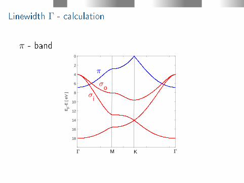
Linewidth Γ - calculation
π - band
18
16
14
12
10
8
6
4
2
0
EF-E
[ eV
]
i
o
KM
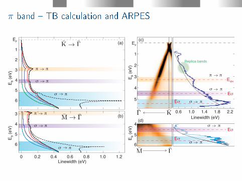
π band TB calculation and ARPES
EB (
eV
)
1
2
3
4
5
EVH
Linewidth (eV)
(a)
5
4
6
EB (
eV
)
EF
(c)
(d)
Replica bands
σ π
π π
Eσ
Eσσ π
Eσ
Eσ
σ π
σ π
0.6 1.0 1.4 1.8 2.2
EB (
eV
)
1
2
3
4
5
EF
6
0.6 0.8 1.0 1.20 0.2 0.4Linewidth (eV)
σ π
π π
σ π
EB (
eV
)
3
4
5
6
σ π
π π
σ π
(b)
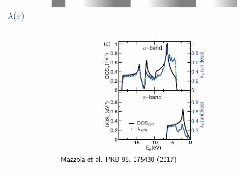
λ(ε)
Mazzola et al. PRB 95, 075430 (2017)

λ =⇒ Tc
The σ band lies far from the Fermi level and does not contribute tographene's transport properties. What would happen if the σ bandcould be shifted to the Fermi level? McMillan formula (W. L.
McMillan PRB 167, 331 (1968) , corrected by Allen (P. B. Allen et al.
PRB 12, 905 (1975) and valid for λ < 1.5),
Tc =~ωlog
1.20exp
(− 1.04(1 + λ)
λ− µ∗(1 + 0.62λ)
), (10)
Eective Coulomb repulsion for s and p band superconductorsµ∗=0.1 (D. M. Gaitonde et al., Bull. Mater. Sci.26, 137 (2003)), thelogarithmically averaged phonon frequency ωlog ≈ 91 meV (Chen Si,
et al.Phys. Rev. Lett. 111, 196802 (2013)) and 0.8 < λ < 1.0, wepredict 49 K < Tc < 72 K.
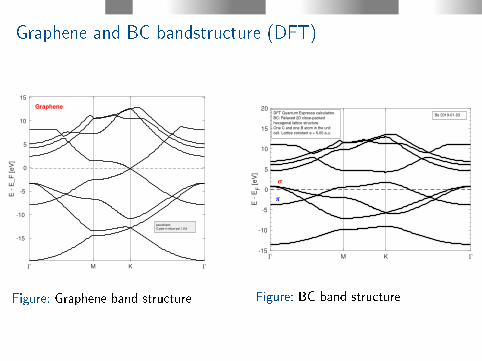
Graphene and BC bandstructure (DFT)
M K
-15
-10
-5
0
5
10
15
E -
E_F
[eV
]
Graphene
pseudopot:
C.pbe-n-rrkjus-psl.1.0.0
Figure: Graphene band structure
M K-15
-10
-5
0
5
10
15
20
E -
EF [
eV
]
Bo 2019-01-03DFT Quantum Espresso calculation.
BC: Relaxed 2D close-packed
hexagonal lattice structure.
One C and one B atom in the unit
cell. Lattice constant a = 5.05 a.u.
Figure: BC band structure

Remarks
Substrate inuence on the electron structure ?
We might expect that the π bands would be most stronglyinuenced by the presence of a substrate, as their wave functionsare built up by the 2pz orbitals pointing towards the substrate.It is well established that a carbon buer layer or zeroth layer(which resembles graphene but with a very strong substrateinteraction and modied π band) is formed directly on top of SiCduring graphene growth. Continued growth (as is relevant for oursamples) results in the formation of the rst true layer of graphene,which is found to be only weakly bonded to the underlying buerlayer (Matthaus et al., PRL 99, 076802 (2007), Varchon et al.,
PRL 99, 126805 (2007) , Kageshima et al., Appl. Phys. Express 2,
065502 (2009) ).

The weak substrate interaction may rigidly shift the electronicstructure of graphene (i.e. as a result of charge transfer), and thenew periodicities present can also create replica bands (Nakatsujiet al., PRB 82, 045428 (2010) ).First principles band structure calculations show no signicantdeviations in comparison with calculated band structure forunsupported graphene. (Varchon et al., PRL 99, 126805 (2007) ).Finally, it is worth noting that even in the case of graphene-onmetal, where the substrate interaction can be relatively strong, thegraphene band structure deviates very little from the rigidly shiftedbandstructure of unsupported graphene (Sutter et al., PRB 80,
245411 (2009), Sutter et al., AM. Chem. Soc. 132, 8175 (2010) ).For these reasons we consider the electron structure forunsupported graphene to be a reasonable rst approximation.
Is the parameter setting of the model potential (V0 and α)rubust ?

Master thesis projects
I Graphene: Find a scheme to optimize the choise of modelone-electron potential and its parameters (presently aGaussian: V0 and α) based on the TB parameters from thelitterature or determined from DFT based calculations.Minimize the error |(Hnm(V0, α)−H0
nm)/H0nm|, where Hnm
and H0nm are the calculated and reference two center
Hamiltonian integral, respectively. EPC linewidth calculations.Collaboration with T. Frederiksen, DIPC, San Sebastian.
I BC: Investigate Boron carbide BC, (every second C atom ingraphene is replaced by a Bohr atom). Find out how the TBparameters and force constants of graphene should bechanged. Calculate the Lifetime broadening. Collaborationwith T. Frederiksen, DIPC, San Sebastian.

Requirements: Quantum mechanics, Solid State Physics (electronstructure and phonons), Tight binding (TB) method for electronstructure and Force constant model for phonons, some experiencewith DFT calculation, some skill in coding; Python, Fortran,Matlab etc


