A fairly sophisticated description of electron-phonon superconductivity has existed since theearly 1960’s, following the work of Eliashberg [1], Nambu [2], Morel and Anderson [3], andSchrieffer et al. [4]. All of this work extended the original ideas of Bardeen, Cooper, andSchrieffer [5] on superconductivity, to include dynamical phonon exchange as the root causeof the effective attractive interaction between electrons in a metal. For certain supercon-ducting materials, Eliashberg theory (as this description is generally called) provides a veryaccurate description of the superconducting state. Nonetheless, as B.T. Matthias was fondof iterating [6], this description was never considered (by him and others) particularly help-ful for discovering new, high temperature superconductors [7]. Part of the problem remainsthat a truly accurate description of the normal state has not been forthcoming. Part of thatproblem is the ‘curse’ of Fermi Liquid Theory. To the extent that the electron-phonon cou-pling causes relatively innocuous corrections to most normal state properties, its underlyingcharacteristics remain undetectable (indeed, as will be reviewed here, the characteristics ofthe electron-phonon interaction are made more apparent in the superconducting state). Anexception may be the A15 compounds, whose anomalous normal state properties might helpus achieve further understanding of the electron-phonon interaction in these materials [10].
This review will barely touch upon normal state properties influenced by the electron-phonon interaction. A considerable literature continues to develop on this topic, includinga more microscopic treatment of model systems with simple electon-ion interactions. Therehave been many theoretical developments in the last two decades, many of which havebeen directed towards understanding the high temperature oxides. Some references will beprovided in the Appendix, but, for the bulk of the chapter, we will focus primarily on the
2
superconducting state in ‘conventional’ superconductors. In the past, many reviews havebeen written on the role of the electron-phonon interaction in superconductors. The readeris directed in particular to the reviews by Carbotte [11], Rainer [12], Allen and Mitrovic[13], and Scalapino [14] (they are listed here in inverse chronological order). While wehave repeated much of what already exists in these reviews, we felt it was important forcompleteness in the present volume, and because the material is presented with a slightlydifferent outlook than has been done in the past.
The first section provides an overview of the subject as we see it, with some detailsrelegated to the Appendix. This is followed by a discussion of our knowledge of the electron-phonon interaction in metals, including an update on old ideas to use the optical conductivityto extract this information. The next two sections provide a very brief review of the impact ofthe electron phonon interaction on the superconducting critical temperature, the energy gap,the specific heat, and critical magnetic fields. The next section examines dynamical responsefunctions. Again, largely because of the discovery of the high temperature superconductors,workers were prompted to re-examine in more detail the effect of stronger electron phononcoupling on various response functions. For example, as will be discussed in the pertinentsubsection, the lack of a coherence peak in the NMR relaxation time was observed. Does this(on its own) indicate an exotic mechanism, or can it be explained by damping effects dueto a substantial electron phonon coupling ? Answers to such questions are reviewed in thissection. Finally, we end with a summary, including some remarks on various non-cuprate butnon-conventional superconductors. The Appendix will sketch some derivations and providereferences to more recent literature.
2 The Electron-Phonon Interaction: Overview
2.1 Historical Developments
The history of superconductivity is an immense and fascinating subject [15]. While thediscovery of superconductivity occurred in 1911 [16], from a theoretical point of view, afirst breakthrough occurred with the discovery of the Meissner-Ochsenfeld effect [17], andthe understanding that this implied that the superconducting state was a thermodynamicphase [18]. During this time a few attempts were made at proposing a mechanism forsuperconductivity [19], but, by 1950, when London’s book [20] appeared, nothing concerningmechanism was really known [21].
In 1950 several important developments took place [22]; first, two independent isotopeeffect measurements were performed on Hg [23, 24], which indicated that the superconduct-ing transition was intimately related to the lattice, probably through the electron-phononinteraction. These experiments were all the more remarkable because in 1922 Onnes andTuyn had looked for an isotope effect in superconducting Pb, and, within the experimentalaccuracy of the time, had found no effect [25].
Secondly, Frohlich [26] adopted, for the first time, a field-theoretical approach to problemsin condensed matter. In particular, he studied the electron-phonon interaction in metals,and demonstrated, through second order perturbation theory, that electrons exhibit an ef-fective attractive interaction through the phonons. Although the theory as formulated was
3
incomplete, it did lay the foundations for subsequent work. In fact one of the essentialfeatures of this mechanism was summarized in his introduction [26]: “Nor is it accidentalthat very good conductors do not become superconductors, for the required relatively stronginteraction between electrons and lattice vibrations gives rise to large normal resistivity.”His theory correctly produced an isotope effect (recognized in a Note Added in Proof), and,moreover, foreshadowed the discovery of the perovskite superconductors, by suggesting thatthe number of free electrons per atom should be reduced.
After hearing about the isotope effect measurements, Bardeen also formulated a theoryof superconductivity based on the electron-phonon interaction, wherein he determined theground state energy variationally [27]. Both of these theories failed to properly explain su-perconductivity, essentially because they focussed on the single-electron self-energies, ratherthan the two-electron instability [22]. Another breakthrough occurred a little later whenFrohlich [28] used a self-consistent method to determine an energy lowering proportional toexp (−1/λ), where λ is the dimensionless electron-phonon coupling constant. This showedhow essential singularities could enter the problem, and why no perturbation expansion inλ would succeed in this problem (although in fact the energy lowering is due to a Peierlsinstability, not superconductivity).
A parallel development meanwhile had been taking place in the problem of electronpropagation in polar crystals, i.e. the study of polarons. In fact, this problem dates backto at least 1933 [29], when Landau first introduced the idea of a “polarization” cloud dueto the ions surrounding an electron, which, among other things, renormalized its properties.Frohlich also addressed this problem, first in 1937 [30], and then again in 1950 [31]. Lee,Low and Pines [32] subsequently took up the problem, also using field-theoretic techniques,to provide a solution to the intermediate coupling polaron problem. This problem was takenon later by Feynman [33], then by Holstein and others [34], along with many others to thepresent day. In fact, as described in the Appendix, a small group of physicists continuesto emphasize polaron physics as being critical to high temperature superconductivity in theperovskites.
Pines, having worked with Bohm on electron-electron interactions, and having just usedfield-theoretic techniques in the polaron problem, now combined with Bardeen to derive aneffective electron-electron interaction, taking into account both electron-electron interactionsand lattice degrees of freedom [35]. The result was the effective interaction Hamiltonianbetween two electrons with wave vectors k and k′ and energies ǫk and ǫk′ [36]:
V effk,k′ =
4πe2
(k − k′)2 + k2
[
1 +h2ω2(k − k′)
(ǫk − ǫk′)2 − h2ω2(k − k′)
]
, (1)
where k is the Thomas-Fermi wave vector, and ω(q) is the dressed phonon frequency. Eq.(1) is an effective interaction; a more formal and general approach, utilizing Green functions,will be given later. Nonetheless, it is clear that this effective interaction captures the essenceof “overscreening”, i.e. for electronic energy differences less than the phonon energy, thephonon contribution to the screened interaction has the opposite sign from the electronicallyscreened interaction, and exceeds it in magnitude. Physically [37], one electron makes atransition, which excites a phonon, accompanied by an ionic charge density fluctuation. Asecond electron undergoes a transition caused by this induced charge density fluctuation. If
4
the differences in the electron energies is small compared to the phonon excitation energy,the second electron is actually attracted to the first. This is shown pictorially in Fig. 1.
Eq. (1) represents the starting point for the two-electron interaction in metals. It was fur-ther simplified for both the Cooper pair calculation [38] and the Bardeen-Cooper-Schrieffer(BCS) [5] calculation. The progression of events that ultimately led to a successful theoryfor BCS has been well documented [22]. Most of this part of the story had little to do withthe details of the attractive mechanism, but rather with the pairing theory itself. Thus,one can divide the theory of superconductivity into two separate conquests: first the estab-lishment of a pairing formalism, which leads to a superconducting condensate, given someattractive particle-particle interaction, and secondly, a mechanism by which two electronsmight attract one another. BCS, by simplifying the interaction, succeeded in establishingthe pairing formalism. They were able to explain quite a number of experiments, previ-ously performed, in progress at the time of the formulation of the theory, and many thatwere to follow. However, one might well ask to what extent the experiments support theelectron-phonon mechanism as being responsible for superconductivity [39]. Indeed, one ofthe elegant outcomes of the BCS pairing formalism is the universality of various properties;at the same time this universality means that the theory really doesn’t distinguish one su-perconductor from another, and, more seriously, one mechanism from another. Fortunately,while many superconductors do display universality, some do not, and these, as it turns out,provided very strong support for the electron-phonon mechanism, as initially motivated byFrohlich [26] and by Bardeen and Pines [35]. Much of this chapter will be concerned withthese deviations from universality.
After the BCS paper appeared, several workers rederived their results using alternativeformalisms. For example, Anderson used an RPA treatment of the reduced BCS Hamiltonianin terms of pseudospin operators [40], and Bogoliubov and others [41, 42] developed moregeneral methods, later to be adapted to inhomogeneous superconductivity by de Gennes[43]. Finally, Gor’kov [44] developed a Green function method, from which both the BCSresults, and the Ginzburg-Landau phenomenology [45] could be derived, near the transitiontemperature, Tc.
The Gor’kov formalism proved to be the most useful, for the purposes of generalizingBCS theory (with its model effective interaction) to the case where the electron-phononinteraction is properly taken into account in the superconducting state. This was done byEliashberg [1], as well as Nambu [2], and later partially by Morel and Anderson [3] and morecompletely by Schrieffer and coworkers [4, 46, 47]. Around the same time tunneling becamea very useful spectroscopic probe of the superconducting state [48]; besides providing anexcellent measure of the gap in a superconductor, it also revealed the fine detail of theelectron-phonon interaction [49], to such an extent that tunneling data could be “inverted”to tell us about the underlying electron-phonon interactions [50]. These developments havebeen well documented in the Parks treatise [51]. In particular retardation effects are coveredin the articles by Scalapino [14] and McMillan and Rowell [52]. An interesting historicalperspective is provided in the article by Anderson [53].
In the meantime, developments in our understanding of the polaron were occurring inparallel. The problem of phonon-mediated superconductivity and the problem of the im-pact of electron-phonon interactions on a single electron are obviously related, but, after the
5
initial work by Frohlich and Pines and coworkers, the two fields seem to have parted ways.Indeed, an excellent summary of the status of polarons at that time is Ref. [54], where,however, there is essentially no “cross-talk” with the theory of superconductivity. Similarly,in the treatise by Parks [51] there is essentially no discussion of polarons [55], in spite of thefact that the ‘polaron’ really is the essential building block of the BCS theory of supercon-ductivity. So, for example, a perusal of the index of the classic texts on superconductivity,by Schrieffer [46], Blatt [56], Rickayzen [57], de Gennes [43], and Tinkham [58] reveals nota single entry [59]. The reason for this is that the electron-phonon coupling strength in allknown superconductors was deemed to be sufficiently weak that the only effect on normalstate properties was a slightly increased electron effective mass. Thus, the electronic state ispresumed to be well described by Fermi Liquid Theory, upon which the BCS theory (and itsmodifications) is based. It is important to keep this in mind; for this reason we will refrainfrom referring to Eliashberg theory as a strong coupling theory (we ourselves have used thisterm in the past). Eliashberg theory goes beyond BCS theory because it includes retardationeffects; however, it is still a weak coupling theory, in the sense that the Fermi energy is thedominant energy, and the quasiparticle picture remains intact.
We make this distinction because in recent years polaron theory has experienced a re-naissance, and some attempts to explain high temperature superconductivity have utilizedpolaron and bipolaron concepts. The bipolaron is simply a bound state of two polarons,analogous to the Cooper pair, except that the latter requires a Fermi sea to exist (at leastin three dimensions) whereas the former exists as a tightly bound pair in the absence of aFermi sea. In this respect bipolaron theories resemble the quasichemical theory advocatedby Schafroth and coworkers [56, 60] in the 1950’s. Tightly bound electron pairs are now rec-ognized as the strong coupling limit of the BCS ground state; the transition to the normalstate is, however, governed by very different (and as yet undetermined) excitations comparedto BCS theory. We will refer to some of this work in the course of this chapter.
To complete this brief historical tour, we should add that in 1964, with the suggestion ofa theorist [61], what has emerged as a new class of superconductors was discovered [62]. Theactual superconducting compound was doped Strontium Titanate (SrTiO3), a perovskitewith low carrier density. This compound, along with BaPb0.75Bi0.25O3, another doped per-ovskite discovered in 1975 [63] with a transition temperature of 12 K, were the precursorsto the modern high temperature superconductors discovered by Bednorz and Muller [8].In fact, with fortuitous foresight, Schooley et al. [64] remarked, “If SrTiO3 had magneticproperties, a complete study of this material would require a thorough knowledge of all ofsolid state physics.” Little did they know that in 1986 perovskites would be discovered, thatnot only had high superconducting transition temperatures, but also exhibited a plethoraof magnetic phenomena. We should also note that the so-called cuprates, which presentlyexhibit superconducting transition temperatures up to 160 K (under pressure), all containCuO2 layers, whereas the cubic oxides (such as SrTiO3, BaPb0.75Bi0.25O3, and Ba1−xKxBiO3
[65] (with Tc ≈ 30 K)) do not. For this reason many workers have come to regard the layeredcuprates and the cubic oxides as belonging to two completely separate (and unconventional)classes, even though they are both essentially low carrier density perovskites.
6
2.2 Electron-Ion Interaction
2.2.1 Overview
A useful ab initio theory has to begin from some fundamental starting point. In condensedmatter systems the starting point is usually taken to be electrons and ions (with theircharges, and masses, etc.) along with the chemical composition of the material [12]. Giventhese ingredients, the prescription for calculation is, in principle, straightforward. One hasto solve the many-body Schrodinger equation, with a Hamiltonian consisting of one-bodykinetic energy terms and the two-body Coulomb interaction. The form of these terms, alongwith all the constants involved, are known, so all that is required to solve the problem isperhaps some ingenuity along with unlimited computer resources. This has been referred toby Laughlin as the Condensed Matter version of “The Theory of Everything” [66].
Of course the difficulty is that, even if one could solve this problem, one would notrecognize what the solution represented. The notion of ionic collective modes (i.e. phonons),for example, would not be very transparent in such an approach. More obscure still wouldbe the distinction between a superconducting state versus a metallic state.
Instead, an approach which separates the complex many-body problem into smaller, moretractable pieces, has traditionally been adopted in condensed matter, and in particular in theproblem of superconductivity [5, 12, 14]. The most systematic approach has been discussedby Rainer [12]. The premise in this approach is the observation that many metals (amongstwhich many undergo a transition to a superconducting state) are well described by LandauFermi Liquid Theory. This allows for an asymptotic expansion in small parameters likekBTc/EF , hωphon/EF and 1/kF ℓ, where EF (kF ) is the Fermi energy (wavevector), ωphon is atypical phonon frequency, and ℓ is the electron mean free path. He separates the problem intothe “high energy problem” (effect of Coulomb interactions amongst the electrons themselvesas well as between the electrons and the fixed nuclear potentials), and the “low energyproblem” (the dressing of conduction electrons with phonons), and the eventual formationof the superconducting state. Most of this review will concern the low energy problem.In our opinion the high energy problem is not at all solved at present, from a truly “abinitio” approach. For example, strictly speaking, one cannot rely on any of the expansionparameters mentioned above, because one does not know, in principle, whether one hasa metal with a well-defined Fermi surface, to begin with. Nonetheless, by appealing toexperimental observation, one can use for many cases the fact that nature has already solvedthe high energy problem, and proceed from there to solve the low energy part. This has beenthe dominant philosophy throughout most of the last four decades towards understandingsuperconductivity.
The difficulty with this approach was exemplified by the discovery of superconductivityin the layered perovskites; band structure calculations for the parent compound (La2CuO4)demonstrated that it was a metal, when in fact the real material was an antiferromagneticinsulator. This problem was later repaired [67], but it remains the case that band structurecalculations fail to properly take into account strong Coulomb correlations, and remainsomewhat powerless to reliably predict a breakdown of the Fermi Liquid picture.
With these caveats, the “ab initio” approach of Ref. [12] has experienced excellent successin cases where a metallic state is known to exist, and experimental input has been used in
7
the theory. We will comment in particular on the “low energy” part of the theory later inthis chapter. A thorough discussion is available in Ref. [12].
2.2.2 Models
The net result of a proper handling of the “high energy” problem in the case of a well-behaved metal is a set of input parameters for the low energy problem that are simple enoughto make the remaining part of the problem appear to have arisen from a non-interactingmodel. The distinction is that the input parameters (band structure, phonon spectrum,etc.) come not directly from specified model parameters, but rather from previous calculationand/or experiment. For this reason, we now discuss possible models for the electron-phononinteraction, which, for the moment, we view as fundamental models in their own right, andnot as models which somehow parameterize (and disguise) the “high energy problem”.
The reason for this is that we hope to accomplish several tasks simultaneously. First, wewill in effect work through the “low energy problem” discussed in the previous subsection.Secondly, we will touch upon some of the more recent work on electron-phonon Hamiltonians,which are characterized not so much by comparison with experiment as comparison withsome “exact” solution, as attained, for example, by Quantum Monte Carlo methods [68, 69].Thirdly, we will also be able to make contact with recent ongoing work on the polaron (andbipolaron). These latter two topics are presented here more by way of a digression. Somefurther detail is presented in an Appendix, but for a more thorough discussion the citedliterature will have to be consulted.
It is always tempting to immediately compare the results of a calculation with experiment;agreement justifies the starting model (in this context this would mean the Hamiltonian, withassociated parameters), whereas disagreement would tend to rule out the starting model asa candidate. In the many-body problem, however, life is not so simple. For one thing,we know the starting Hamiltonian, as emphasized in the previous subsection. We will getagreement with experiment if we were only able to routinely calculate any observable. How-ever, in our endeavour to understand many-body systems, we have grown to utilize effectiveHamiltonians, which would capture the essence of the phenomenon under investigation. Thepurpose of this strategy is twofold; we make sense of the many-body system in terms we canunderstand, and we make the calculation itself more tractable in practice.
There are many Hamiltonians in condensed matter physics, which were derived as effec-tive Hamiltonians for some particular problem, but, which have since taken on a life of theirown. This is true because (a) they have withstood solution in spite of their simplicity, and(b) they epitomize some qualitative aspect of the more general problem. Famous examplesare the Heisenberg/Ising model for spins, and the Hubbard model for fermions with spindegrees of freedom. In the electron-phonon problem several effective models have arisen overthe years, the three most prominent of which have been the Frohlich Hamiltonian [26], theHolstein model [34], and the BLF (Barisic-Labbe-Friedel) model [70] (also known as the SSH(Su-Schrieffer-Heeger) model [71]). The Frohlich Hamiltonian was derived in a continuumapproximation (see Ref. [72] or [73] for a derivation), and results in a coupling betweenthe electron density and the ionic momentum (a canonical transformation changes this tothe ionic displacement) which diverges as the momentum transfer between electron and ions
8
goes to zero. This Hamiltonian has been the subject of many investigations of the polaron.Holstein proposed his model as a simplification in which the interaction between electron andion is more local; in fact in some ways the simplification Hubbard [74] invoked to replace thelong-range Coulomb interaction is analogous to the simplification that the Holstein modelrepresents compared to the Frohlich Hamiltonian. Both the Frohlich and Holstein modelsrepresent couplings of the electron to an optical phonon mode. We will focus on the Hol-stein model since it is particularly amenable to numerical simulations. In contrast, the BLF(SSH) model couples the electron to the relative displacement of nearby ions, i.e. an acousticphonon mode. The physics is simple; in the Holstein model ionic distortions affect the elec-tron energy level at a particular site, while in the BLF model ionic displacements affect theelectron hopping amplitude. These are represented pictorially in Fig. 2, although of coursethe coupling is dynamic.
The BLF model gained prominence in the 1980’s [75] when it was used to describesolitons in conducting polymers; otherwise comparatively little effort has been expendedtowards an understanding of its properties, particularly in two or three dimensions. TheBLF Hamiltonian is
H =∑
i
p2i
2M+
∑
<ij>
1
2K(ui − uj)
2
−∑
<ij>
σ
(tij − α · (ui − uj)(c†iσcjσ + h.c.), (2)
where the first line refers to the ions, with mass M and spring constant K. The ionicdegrees of freedom are described by the ion momentum, pi, and displacement, ui, at site i.The electrons are described by creation (annihilation) operators c†iσ (ciσ) for an electron withspin σ at site i. The electron hopping amplitude is given by tij ; this in turn is modulatedby ionic vibrations, and therefore results in the electron-ion coupling with strength |α|. Thecoupling constant |α| is proportional to the gradient of the hopping overlap integral betweenelectron orbitals on two neighbouring sites.
Equation 2 gives rise to the standard electron-phonon Hamiltonian, as written in mo-mentum space:
H =∑
kσ
ǫkc†kσckσ +
∑
q
hωqa†qaq +
1√N
∑
kk′
σ
g(k,k′)(ak−k′ + a†−(k−k′))c†k′σckσ. (3)
We have used the conventional oscillator operators, aq = Mωq
2h(uq + ipq) and the standard
Fourier expansions, c†iσ = 1√N
∑
k eik·Ric†kσ, etc. The phonon dispersion is given by ωq, where,
in principle, q includes branch indices as well as momenta within the first Brillouin zone,and g(k,k′) is the coupling function. For the BLF Hamiltonian, this coupling function hasa very specific form (involving sine functions). A more general consideration of the electron-ion interaction yields a Hamiltonian of essentially the same form [13, 14], but where theparameters involved are understood to already contain the “high energy” effects alludedto earlier. State-of-the-art computations of the electron-ion coupling strength, are given,for example, in Ref. [76] (for La2−xSrxCuO4) and in Ref. [77] (and references therein, forA3C60).
9
The Holstein Hamiltonian is
H = −t∑
<ij>
σ
(c†iσcjσ +H.c.) +∑
i
[p2
i
2M+
1
2Kx2
i ] − α∑
iσ
xiniσ, (4)
where the parameters are as before except that the displacement variable xi represents the(one-dimensional) displacement of some optical mode (say a breathing mode) associatedwith the ith site, and the electron-ion coupling α represents the change in site energy (perunit displacement) associated with this mode. In momentum space this Hamiltonian isparticularly simple:
H =∑
kσ
ǫkc†kσckσ +
∑
q
hωEa†qaq +
g√N
∑
kq
σ
(aq + a†−(q))c†k+qσckσ, (5)
where ωE is the Einstein mode frequency and g ≡√
α2hωE
2K. This model has been studied
extensively in the last twenty years, at least partly due to its simplicity. Some of this workis reviewed in the Appendix.
2.3 Migdal Theory
The primary language of many-body systems is the Green function, or propagator. Manybooks have been written (see for example Refs. [78–83]) about the Green function formalism,so we will bypass a thorough discussion here. A sketch of the derivation of the Migdal [84]equation for the electron self-energy is given in the Appendix. Migdal argued that all vertexcorrections are O(m/M)1/2 compared to the bare vertex, and therefore can be ignored. Herem (M) is the electron (ion) mass. This represents a tremendous simplification, and allowsone to solve a theory which should work for arbitrary coupling strength (this is, in fact, notthe case, for reasons that will become apparent in the next section).
An “exact” formulation of the electron-phonon problem can be summarized [84–86] interms of the Dyson equations (written in momentum and imaginary frequency space):
G(k, iωm) = [G(k, iωm)−1 − Σ(k, iωm)]−1 (6)
for the electron, andD(q, iνn) = [D(q, iνn)−1 − Π(q, iνn)]−1 (7)
for the phonon, where G(k, iωm) is the one-electron Green function, D(q, iνn) is the phononpropagator, and Σ(k, iωm) is the electron and Π(q, iνn) the phonon self energy. Then,
gk,k+qG(k + q, iωm + iνn)G(k, iωm)Γ(k + q, iωm + iνn;k, iωm;q, iνn),
(9)
10
where the vertex function Γ can only be defined in terms of an infinite set of diagrams (i.e.not in closed form).
The non-interacting propagators are
G(k, iωm) = [iωm − (ǫk − µ)]−1 (10)
for the electron andD(q, iνn) = [−M(ω2(q) + ν2
n)]−1 (11)
for the phonon, where ǫk is the single electron dispersion (band indices are implicit here andin the following), µ is the chemical potential, and ω(q) is the phonon dispersion. In writingthese relations we have adopted the finite temperature Matsubara formalism, with Fermion(iωm ≡ iπT (2m− 1)) and Boson (iνn ≡ i2πTn) Matsubara frequencies, where m and n areintegers and T is the temperature (kB ≡ 1). The Matsubara sums in Eqs. (8,9) extend overall integers, and the momentum sums extend over the first Brillouin zone. This conventionwill be maintained unless noted otherwise.
Migdal’s approximation was to set the vertex function Γ equal to the bare vertex, g.Then, the electron self-energy can be written:
Σ(k, iωm) = − 1
Nβ
∑
k′,m′
|gk,k′|2D(k − k′, iωm − iωm′)G(k′, iωm′). (12)
Migdal [84] also included renormalization effects in the phonon propagator. With an appli-cation to real materials in mind, however, the electron dispersion relations will have beenobtained from a band structure calculation, and the phonon properties will generally havebeen taken from experiment. In this case the phonon self energy is omitted entirely (to avoiddouble counting). In addition electron-electron effects have been omitted, as they have beenpresumed to be included already in the band structure and phonon calculations (to the bestextent possible).
Alternatively, Eq. (12) can be viewed as having been derived from some microscopicelectron-ion Hamiltonian. For example, in the case of the Holstein Hamiltonian, Eq. (4),gk,k′ → g, the constant appearing in Eq. (5), and the electron band structure is given byǫk = −2t cos (kx) (in one dimension, and for nearest-neighbour hopping only). In addition,the phonon frequency becomes dispersionless (ω(q) → ωE) and the phonon self energy isgiven by some appropriate approximation. Such an identification is useful for comparison toexact results (usually done numerically - see the Appendix for references).
In the classical literature [13, 84, 85, 87, 88], Eq. (12) is simplified in the following way.First, very often the phonon propagator is provided separately, usually by inelastic neutronscattering measurements [89, 90]. To see how, one first writes the phonon propagator interms of its spectral representation [13]:
D(q, iνn) =∫ ∞
0dνB(q, ν)
2ν
(iνn)2 − ν2(13)
where B(q, ν) is the phonon spectral function
B(q, ν) ≡ −1
πImD(q, ν + iδ). (14)
11
The spectral function is positive definite, and obeys a sum rule; it is the quantity thatis constructed with fits to high-symmetry phonon dispersion curves measured by inelasticneutron scattering [89]. Following this tact a calculation of the phonon self energy is nolonger required. Another simplification was recognized in Ref. [85]; this is the use of thenon-interacting electron Green function G(k, iωm) in the right hand side of Eq. (12) insteadof the full self-consistent choice, G(k, iωm). This approximation is valid when particle-hole symmetry is present and the infinite bandwidth approximation is invoked. This latterapproximation is used extensively in the early literature on metals and superconductors; asystematic explanation of the logic is provided in Ref. [13], and requires the usual hierarchyof energy scales, ωphon << EF (h ≡ 1). The result is
Σ(k, iωm) =1
Nβ
∑
k′,m′
∫ ∞
0dν|gk,k′|2B(k − k′, ν)
2ν
(ωm − ωm′)2 + ν2G(k
′, iωm′). (15)
The form of Eq. (15) allows one to introduce the electron-phonon spectral function,
α2F (k,k′, ν) ≡ N(µ)|gk,k′|2B(k − k′, ν), (16)
where N(µ) is the electron density of states at the chemical potential. At this point onecan introduce ‘Fermi surface Harmonics’ [13, 91], and define an electron self-energy withFermi momentum which depends on Matsubara frequency, and on the angle around theFermi surface. Elastic impurities would act to homogenize the self-energy (as well as otherproperties), so a more useful function for dirty superconductors is the Fermi-surface-averagedspectral function,
α2F (ν) ≡ 1
N(µ)2
∑
k,k′
α2F (k,k′, ν)δ(ǫk − µ)δ(ǫk′ − µ). (17)
To gain an understanding of electron-phonon effects, Englesberg and Schrieffer [85] solvedthis model for two simple phonon models, the Einstein and Debye models. Here we summa-rize their results for the Einstein model, with unmodified phonon spectrum, a simpler casesince both the phonon spectrum and the bare vertex function are independent of momentum.In this case gk,k′ ≡ g and B(q, ν) ≡ δ(ν − ωE). Using, in addition, the prescription
1
N
∑
k
→∫
dǫN(ǫ) (18)
along with a constant density of states approximation, extended over an infinite bandwidth,one obtains for the electron self energy
Σ(iωm) = λω2E
∫ ∞
−∞dǫ
1
β
∑
m′
1
ω2E + (ωm′ − ωm)2
1
iωm′ − (ǫ− µ), (19)
where we have used the standard definition for the electron-phonon mass enhancement pa-rameter, λ:
λ ≡ 2∫ ∞
0dνα2F (ν)
ν, (20)
12
which, for the Einstein spectrum used here, reduces to
λ = 2N(ǫF )g2/ωE . (21)
Performing the Matsubara sum yields
Σ(iωm) =λωE
2
∫ ∞
−∞dǫ(
n(ωE) + 1 − f(ǫ− µ)
iωm − ωE − (ǫ− µ)+
n(ωE) + f(ǫ− µ)
iωm + ωE − (ǫ− µ)
)
(22)
where f(ǫ − µ) is the Fermi function and n(ωE) is the Bose distribution function. Theremaining integral can also be performed [13]
Σ(z) =λωE
2
[
−2πi(n(ωE) + 1/2) + ψ(1
2+ i
ωE − z
2πT) − ψ(
1
2− i
ωE + z
2πT)]
(23)
where ψ(x) is the digamma function [13, 92] and the entire expression has been analyticallycontinued to a general complex frequency z. Because we performed the Matsubara sum first,before replacing iωm with z, this is the physically correct analytic continuation [93].
At zero temperature one can use well-documented properties of the digamma function,or, more simply, refer to the analytic continuation of Eq. (22), since the Bose and Fermifunctions may be more familiar. Since n(ωE) → 0 and f(ǫ− µ) → θ(µ − ǫ) as T → 0 (θ(x)is the Heaviside step function), the self energy at T = 0 is
Σ(z) =λωE
2ln(
ωE − z
ωE + z
)
. (24)
Spectroscopic measurements yield properties as a function of real frequency; because of theanalytic properties of the Green function, this corresponds to a frequency either slightlyabove or below the real axis. We will use frequencies slightly above, and designate theinfinitesmal positive imaginary part by ‘iδ’. Thus,
Σ(ω + iδ) =λωE
2
[
ln | ωE − ω
ωE + ω| −iπθ(| ω | −ωE)
]
. (25)
The real and imaginary parts of this self energy are shown in Fig. 3, along with the non-interacting inverse Green function (ω−(ǫk−µ)) to determine the poles of the electron Greenfunction (see Eq. (6)) graphically. A quantity often measured in single particle spectroscopiesis the spectral function, A(k, ω) defined by
A(k, ω) ≡ −1
πImG(k, ω + iδ). (26)
With this definition, we obtain, through Eq. (6) and (25),
A(k, ω) = δ(
ω − (ǫk − µ) − λωE
2ln | ωE − ω
ωE + ω|)
if | ω |< ωE,
=λωE/2
(
ω − (ǫk − µ) − λωE
2ln | ωE−ω
ωE+ω|)2
+(
πλωE
2
)2 if | ω |> ωE . (27)
13
Plots are shown in Fig. 4. Each spectral function displays a quasiparticle peak, whosestrength ak and frequency ωk is implicitly dependent on wavevector
ak =(
1 +λ
1 − (ωk/ωE)2
)−1
, (28)
where ωk is the solution (between −ωE and ωE) to the zero of the delta-function argumentin Eq. (27). For all momenta (or equivalently all ǫk−µ) there is a solution, whose frequencyapproaches ωE asymtotically as ǫk − µ → ∞. The weight of this peak starts at the Fermisurface (ǫk = µ) as 1/(1+λ) and quickly goes to zero according to Eq. (28) as ωk → ωE, whichoccurs for ǫk
>∼2ωE . For larger ǫk a quasiparticle peak forms once again, albeit with non-
zero width, at approximately the non-interacting electron energy, ǫk = µ. At intermediateǫk ≈ ωE, the quasiparticle picture has broken down, and a description as described here isrequired for a complete picture.
How well the Migdal approximation works in specific circumstances is the subject of on-going research (see, for example, Refs. [94–98], and the Appendix. For example, Alexandrovet al. [99] found an apparent breakdown (for coupling strengths greater than 1, within theHolstein model) to the approximation when a finite electronic bandwidth was taken intoaccount.
We have focussed on the modifications to the electron spectral function due to theelectron-phonon interaction. For excitations at the Fermi level (ǫk = µ), the quasiparti-cle pole remains there (ωkF
= 0), remains infinitely long-lived (it is a delta-function), buthas a reduced weight, by a factor of 1 + λ. This same factor enhances the effective mass,and alters various normal state properties in a similar way [88, 100]. For example, the lowtemperature electronic specific heat is linear in temperature with coefficient usually denotedby γ, which is proportional to the electron density of states. The electron-phonon interactionenhances this coefficient by the same factor, 1 + λ. Other renormalizations are reviewed inRef. [88].
2.4 Eliashberg Theory
Eliashberg theory is the natural development of BCS theory to include retardation effects dueto the ‘sluggishness’ of the phonon response. In fact, insofar as BCS introduced an energycutoff, ωD (the Debye frequency), they included, in the most minimal way, retardation effects.However, Eliashberg theory goes well beyond this approximation, and handles momentumcutoffs and frequency cutoffs separately. We begin this section with a very brief review ofBCS theory, followed by a more detailed discussion of Eliashberg theory.
2.4.1 BCS Theory
Before one establishes a theory of superconductivity, one requires a satisfactory theory ofthe normal state. In conventional superconductors, Fermi Liquid Theory appears to workvery well, so that, while we cannot solve the problem of electrons interacting through theCoulomb interaction, experiment tells us that Coulomb interactions give rise to well-definedquasiparticles, i.e. a set of excitations which are in one-to-one correspondence with those
14
of the free-electron gas. The net result is that one begins the problem with a ‘reduced’Hamiltonian,
Hred =∑
kσ
ǫkc†kσckσ +
∑
kk′
Vk,k′c†k↑c†−k↓c−k′↓ck↑, (29)
where, for example, the electron energy dispersion ǫk already contains much of the effect dueto Coulomb interactions. The important point is that well-defined quasiparticles with a well-defined energy dispersion near the Fermi surface are assumed to exist, and are summarizedby the dispersion ǫk. The pairing interaction V (k,k′) is assumed to be ‘left-over’ from themain part of the Coulomb interaction, and this is the part that BCS simply modelled, basedon earlier work by Frohlich [26] and Bardeen and Pines [35].
Complete derivations of BCS theory have been provided elsewhere in this volume; herewe state the final result [46]:
∆k = − 1
N
∑
k′
Vk,k′
∆k′
2Ek′
tanhβEk′
2, (30)
whereEk =
√
(ǫk − µ)2 + ∆2k (31)
is the quasiparticle energy in the superconducting state, and ∆k is the variational parameterused by BCS. An additional equation which must be considered alongside the gap equation(30) is the number equation,
n = 1 − 1
N
∑
k
ǫk − µ
Ek
tanhβEk
2. (32)
Given a pair potential and an electron density, one has to ‘invert’ these equations to determinethe variational parameter ∆k and the chemical potential. For conventional superconductorsthe chemical potential hardly changes on going from the normal to the superconductingstate, and the variational parameter is much smaller than the chemical potential, with theresult that the second equation was usually ignored.
BCS then modelled the pairing interaction as a negative (and therefore attractive) con-stant with a sharp cutoff in momentum space:
Using this potential in Eq. (30), along with a constant density of states assumption over theentire range of integration, we obtain
1
λ=∫ ωD
0
dǫ
Etanh
βE
2, (34)
where λ ≡ N(µ)V . At T = 0, the integral can be done analytically to give
∆ = 2ωDexp (−1/λ)
1 − exp (−1/λ). (35)
15
In weak coupling this becomes the more familiar
∆ = 2ωD exp (−1/λ), (36)
while in strong coupling we obtain∆ = 2ωDλ. (37)
Both of these results are within the realm of BCS theory (at zero temperature) [101, 102],although the latter generally requires a self-consistent solution with the number equation,Eq. (32).
Close to the critical temperature, Tc, the BCS equation becomes
1
λ=∫ βωD/2
0dx
tanh x
x, (38)
which can’t be solved in terms of elementary functions for arbitrary coupling strength.Nonetheless, in weak coupling, one obtains
Tc = 1.13ωD exp (−1/λ), (39)
and in strong couplingTc = ωDλ/2. (40)
It is clear that Tc or the zero temperature variational parameter ∆ depend on material prop-erties such as the phonon spectrum (ωD), the electronic structure (N(µ)) and the electron-ioncoupling strength (V ). However, it is possible to form various thermodynamic ratios, whichturn out to be independent of material parameters. The obvious example from the precedingequations is the ratio 2∆
kBTc. In weak coupling (most relevant for conventional superconduc-
tors), for example, we obtain2∆
kBTc= 3.53, (41)
a universal result, independent of the material involved. Many other such ratios can bedetermined within BCS theory, and the observed deviations from these universal valuescontributed to the need for an improved formulation of BCS theory. For example, theobserved value of this ratio in superconducting Pb was closer to 4.5, a result that is readilyunderstood with Eliashberg theory. It is worth noting that simply extending BCS theory tothe strong coupling limit (see Eqs. (37,40) above) results again in a universal constant, 2∆
kBTc=
4, which is the maximum value attainable within BCS theory with a constant interaction[103], and is still clearly too low.
Other aspects of BCS theory, particularly those which prove to inadequately account forthe superconducting properties of some materials (notably Pb and Hg) will not be reviewedhere. Instead, we will make reference to the BCS limit as we encounter various propertieswithin the experimental or Eliashberg context.
16
2.4.2 Eliashberg Equations
In most reviews and texts that derive the Eliashberg equations, the starting point is theNambu formalism [2]. While this formalism simplifies the actual derivation, it also providesa roadblock to further understanding for the uninitiated. For this reason we have followed theconceptually much more straightforward approach (provided by Rickayzen [57], for example)in the derivation outlined in the Appendix. The result can be summarized by the followingset of equations:
Σ(k, iωm) ≡ 1
Nβ
∑
k′,m′
λkk′(iωm − iωm′)
N(µ)G(k′, iωm′) (42)
φ(k, iωm) ≡ 1
Nβ
∑
k′,m′
[
λkk′(iωm − iωm′)
N(µ)− Vkk′
]
F (k′, iωm′), (43)
G(k, iωm) =G−1
n (k, iωm)
G−1n (k, iωm)G−1
n (−k,−iωm) + φ(k, iωm)φ(k, iωm)(44)
F (k, iωm) =φ(k, iωm)
G−1n (k, iωm)G−1
n (−k,−iωm) + φ(−k,−iωm)φ(−k,−iωm)(45)
G−1n (k, iωm) = G−1
(k, iωm) − Σ(k, iωm). (46)
Another couple of equations identical to Eqs. (43) and (45), except with φ and F instead ofφ and F , have been omitted; they indicate that some choice of phase is possible, which willbe important for Josephson effects [104] but not for what will be considered in the remainderof this chapter. Therefore, we use φ = φ [105].
Note that G−1 (k, iωm) is the inverse of the non-interacting Green function, in which
Hartree-Fock contributions from both the electron-ion and electron-electron interactions areassumed to be contained.
Following the standard practice we have used a kernel given by
λkk′(z) ≡∫ ∞
0
2να2kk′F (ν)
ν2 − z2dν (47)
where α2kk′F (ν) is given by Eq. (16). Eqs. (42-47) have been written in a fairly general
way; in this way they can be viewed as having arisen from a microscopic Hamiltonian as inEqs. (2-4) (although electron-electron interactions have been included in the pairing channelonly, and not in the single electron self energy), or, alternatively, from a treatment of realmetals, where, as mentioned earlier, the electron and phonon structure come from previouscalculations and/or experiments. These equations emphasize the electron-ion interaction;attempts to explain superconductivity through the electron-electron interactions have beenproposed in the past, mainly through collective modes [106–113]; some of these attempts willbe treated elsewhere in this volume in the context of high temperature superconductivity.
Assuming the electron and phonon structure is given, Eqs. (42-47) must be solved for thetwo functions, Σ(k, iωm) and φ(k, iωm). The procedure is as follows: it is standard practiceto separate the self energy, Σ(k, iωm), into its even and odd components [13]:
iωm[1 − Z(k, iωm)] ≡ 1
2[Σ(k, iωm) − Σ(k,−iωm)]
17
χ(k, iωm) ≡ 1
2[Σ(k, iωm) + Σ(k,−iωm)] (48)
where Z and χ are both even functions of iωm (and, as we’ve assumed all along, k). Then,Eq. (42) becomes two equations,
These constitute general Eliashberg equations for the electron-phonon interaction, in whichelectron-electron interactions enter explicitly only in the pairing equation. Very completecalculations of these functions (linearized, for the calculation of Tc) were carried out for Nbby Peter et al. [114], and for Pb by Daams [115].
The more standard practice is to essentially confine all electronic properties to the Fermisurface; then only the anisotropy of the various functions need be considered. Often theseare simply averaged over (due to impurities, for example), or the anisotropy may be veryweak and therefore neglected. In this case the equations (49-53) can be written
Zm = 1 + πT∑
m′
λ(iωm − iωm′)(ωm′/ωm)Zm′
√
ω2m′Z2
m′ + φ2m′
A0(m′) (54)
χm = −πT∑
m′
λ(iωm − iωm′)A1(m′) (55)
φm = πT∑
m′
(
λ(iωm − iωm′) −N(µ)Vcoul
)
φm′
√
ω2m′Z2
m′ + φ2m′
A0(m′) (56)
n = 1 − 2πTN(µ)∑
m′
A1(m′) (57)
where we have adopted the shorthand Z(iωm) = Zm, etc, λ(z) and Vcoul represent appropriateFermi surface averages of the quantities involved, and the functions A0(m
′) and A1(m′) are
given by integrals over appropriate density of states, using the prescription (18) to convert
18
from Eqs. (49-53) to Eqs. (54-57). If the electron density of states is assumed to be constant,then, with the additional approximation of infinite bandwidth, A0(m
′) ≡ 1 (actually a cutoff,θ(ωc− | ωm′ |), is required in Eq. (56)), and A1(m
′) ≡ 0. This last result effectively removesχm (and Eqs. (55,57) ) from further consideration. An earlier review by one of us [11]covered the consequences of the remaining two coupled equations in great detail.
Nonetheless, a considerable effort has been devoted to examining gap anisotropy, as wellas variations in the electronic density of states near the Fermi surface. We describe some ofthis work in the following few paragraphs.
Referring back to Eqs. (49-53), one can rewrite the summation over k′ on the right-hand-side of these equations as an integral over energy plus an integral over angle (for agiven constant energy surface). In carrying out the energy integration the energy dependentelectron density of states (EDOS), N(ǫ), introduces a new weighting factor if N(ǫ) exhibitsvariations over the energy scale of the phonon frequencies. On the other hand, the integrationover angle will account for variations of the gap and other quantities in the integrandswith momentum direction. There is a large literature on each of these complicating effects,starting with anisotropy effects [116, 117], and more recently with EDOS energy dependence[13, 118–120].
Concerning anisotropy, the observed universal decrease in Tc with increasing impurityconcentration (i.e. so-called ‘normal’ impurities, deemed to be innocuous by Anderson’sargument [121]) can be attributed to the washing out of gap anisotropy. To see why thisdecreases Tc (we omit here effects due to valence changes) we note that the impurity potentialscattering has a tendency to homogenize the gap on the Fermi surface. This tends to reducethe gap in some directions, and it is these directions that make the maximum contributionto Tc, and so Tc is reduced. A simple BCS calculation can demonstrate this analytically.One makes a separable approximation for the pairing potential, Eq. (33), to be used in theBCS equation (30):
Vk,k′ = −V (1 + ak)(1 + ak′), (58)
where the same energy cutoffs are assumed, and ak is a function of momentum directiononly. Assuming ak to be small with a Fermi surface average equal to zero (i.e. < ak >= 0)and a2
k = a2, with <> denoting an angular average over the Fermi surface, then clearly∆k = ∆(1 + ak). Solving the resulting equation yields
< ∆k >= ∆ = 2ωD exp (− 1
λ(1 + a2))(
1 − 3
2a2)
(59)
in the weak coupling approximation. Similarly, one can solve the Tc equation, to obtain
Tc = 1.13ωD exp (− 1
λ(1 + a2)). (60)
This last equation demonstrates that Tc is increased by anisotropy. Hence, increased scat-tering due to impurities will decrease Tc, as the anisotropy is washed out. Finally, the gapratio,
2 < ∆k >
kBTc= 3.53
(
1 − 3
2a2)
, (61)
19
showing that anisotropy reduces this quantity.How big can the anisotropy be in pure conventional superconductors ? Microscopically
the anisotropy is related to band structure anisotropy plus anisotropy in the electron-phononspectral function from Eq. (16), α2F (k,k′, ν). In Fig. 5 we show the results of a calculationof the gap anisotropy in Pb as a function of position on the Fermi surface [122]. Thesecalculations include multiple-plane-wave effects for the electronic wave functions, and thecorresponding distortions of the Fermi surface from a sphere, as well as anisotropy effectsdue to the phonons and umklapp processes in the electron phonon interactions. The Figureillustrates the gap ∆(θ, φ) at zero temperature, as a function of θ for three constant φ arcs.Solid angle regions where the Fermi surface of Pb does not exist are indicated by verticalsolid lines. It is clear that the pure Pb crystal gap is highly anisotropic, varying by about20% over the Fermi surface. As described above, impurities will wash out this anisotropy.Nevertheless, such anisotropies can be observed in some low temperature properties, like thespecific heat. For more details the reader is referred to Ref. [117].
The other complication we have mentioned is an energy variation in the EDOS, as seemsto exist in some A15 compounds. If this energy dependence occurs on a scale comparableto ωD, then N(ǫ) cannot be assumed to be constant, and cannot be taken outside of theintegrals in Eqs. (49-53). Such EDOS energy dependence is thought to be responsible forsome of the anomalous properties seen in A15 compounds — their magnetic susceptibilityand Knight shift [123], and the structural transformation from cubic to tetragonal [124–126].Several electronic band structure calculations [127–130] also find sharp structure in N(ǫ) atthe Fermi level. An accurate description of the superconducting state thus requires a propertreatment of this structure. This was first undertaken to understand Tc by Horsch andReitschel [118] and independently by Nettel and Thomas [119]. A more general approach tounderstanding the effect of energy dependence in N(ǫ) on Tc was given by Lie and Carbotte[120], who formulated the functional derivative δTc/δN(ǫ); they found that only values ofN(ǫ) within 5 to 10 times Tc around the chemical potential have an appreciable effect on thevalue of Tc. More specifically they found that δTc/δN(ǫ) is approximately a Lorentzian withcenter at the chemical potential; the function becomes negative only at energies |ǫ−µ|>∼50Tc.
Irradiation damage experiments illustrate some of this dependency. For example, ir-radiation of Mo3Ge causes an increase in Tc [131]. Washing out gap anisotropy with theirradiation cannot possibly account for an increase in Tc; instead, this result finds a naturalexplanation in the fact that the chemical potential for Mo3Ge falls in a valley [132] of theEDOS, and irradiation smears the EDOS, thus increasing N(µ), and hence Tc.
For details on the formulation of Eliashberg theory with an energy dependent N(ǫ) thereader is referred to the work of Pickett [133] and Mitrovic and Carbotte [134], and referencestherein. The energy dependent EDOS affects many properties. To illustrate a typical resultwe show in Fig. 6 the effect of an energy dependent EDOS on the current (I)-voltage (V)characteristics of a tunneling junction [134, 135]. A detailed discussion of tunneling appearsin Section 3.3.2. The tunneling conductance is proportional to the electron density of states,
and is denoted by σ(ω) ≡ Re
(
ω√ω2−∆2(ω)
)
. Fig. 6 shows the difference with the BCS
conductance, σ(ω)/σBCS(ω)−1 vs. ω−∆ [134, 135]. Fig. 6a (b) is for a peak (valley) in theEDOS at the Fermi level. The solid curves include the effect of an energy dependent EDOS,
20
while the dashed curves do not (the EDOS is approximated by a constant value, N(µ)). Inthese examples the electron phonon spectral density obtained for Nb3Sn [136] is used.
These differences can be highlighted in another way, shown in Fig. 7 [134, 135]. Here,the “effective” electron phonon spectral density, α2F (Ω)eff , is obtained by inverting the solidcurves in Fig. 6 under the assumption that the EDOS is constant and equal to N(µ). Thedashed curves give Shen’s original α2F (Ω) while the solid curves are the result of (incorrectly)inverting the result obtained with an energy dependent EDOS, but not accounting for it inthe inversion process itself. The actual EDOS used to generate the I-V characteristic isshown in the inset for each figure. It contains a peak in Fig. 7a and a valley in Fig. 7b.Clearly a peak introduces a negative tail into α2F (Ω)eff , which of course is not present in theactual α2F (Ω). For other important modifications the reader is referred to the references.The rest of this chapter will focus primarily on the ‘standard’ theory, using Eqs. (54-57)with A0(m) ≡ 1 and A1(m) ≡ 0.
All of the equations discussed so far have been developed on the imaginary frequencyaxis. Because practitioners in the field at the time were interested in tunneling spectroscopymeasurements [49], the theory was first developed on the real frequency axis [4, 47]. Theresulting equations are complicated, even for numerical solution. It wasn’t until quite anumber of years later that numerical work returned to the imaginary axis [137], where, forthermodynamic properties, the numerical solution was very efficient [138–141]. The difficulty,however, was that imaginary axis solutions are not suitable for dynamical properties. We willreturn to the interplay between imaginary and real frequency axis solutions as we ecounterthem throughout the chapter.
3 The Phonons
3.1 Neutron Scattering
When dealing with model Hamiltonians, the phonon dispersion relations (before interactionwith the electrons) are generally given, and simple: they are Einstein modes, or Debye-likemodes, for example. A noteable exception is the case where the model contains anharmonicforces, in which case even the ‘non-interacting’ phonon spectrum is unknown.
In the case of real solids, and in particular metals, the situation is much worse. In thiscase the electrons cannot be ignored, though they can be treated in the Born-Oppenheimerapproximation. Nonetheless the results require parametrization (with input from other ex-periments) and are generally not reliable. Pseudopotential methods [142, 143] can be appliedto this problem, again, with limited success. In contrast, the spectacular success of inelasticneutron scattering techniques [89, 90] to simply measure the phonon dispersion curves in realmetals effectively eliminates the need to calculate them quantitatively. Various qualitativeeffects, like the impact of electronic screening to the long wavelength ionic plasma mode [146],as well as the existence of Kohn anomalies [147], all due to the presence of electrons, areunderstood theoretically. For detailed results, however, Born-von Karman fits to high sym-metry phonon dispersions suffice for an excellent description of the low temperature phononproperties. At temperatures of order 10 K, the phonons in most conventional superconduc-tors are completely determined, and no longer changing with temperature. Hence, as far as
21
understanding (low temperature) superconductivity is concerned, these higher temperaturemeasurements are sufficient.
The measured dispersion curves, ωq (again, branch indices are suppressed), are summa-rized in the frequency distribution
F (ν) =1
N
∑
q
δ(ν − ωq), (62)
where N is the number of ions in the system, and q is a wavevector which ranges over theentire First Brillouin Zone (FBZ), (and implicitly contains the branch index). It should bestressed that this procedure is an idealization; in actual fact a set of ‘constant q’ scans areperformed (usually along high symmetry directions). A typical result [89] is shown in Fig. 8for Pb, for a set of wavevectors along the diagonal in reciprocal space. Note that the neutroncounts tend to form a peak as a function of energy transfer (to the neutron), hν. In generalthese peaks have a finite width, i.e. broader than the spectrometer resolution; these are dueto a variety of effects, for example, anharmonic effects. Nonetheless, because the peaks arerelatively sharp compared to the centroid energy, (i.e. the phonon inverse lifetimes are smallcompared to their energies), these data are usually presented in the form of Fig. 9, as a setof dispersion curves. Fig. 9 does obscure, however, the lifetimes of the various phonons, andhence the validity of Eq. (62), where infinitely long-lived phonons are assumed throughoutthe Brillouin zone, is called into question.
Nonetheless, for most of the Brillouin zone the approximation of infinitely long-livedexcitations is a good one (hence, the name, phonon), and so the spectrum of excitations canbe constructed according to Eq. (62). Such a procedure relies on coherent neutron scattering.An alternative is to use incoherent neutron scattering, whereby one measures the spectrummore or less directly. This latter procedure has advantages over the former, but also includesmultiphonon scattering processes, and for non-elemental materials, weighs the contributionfrom each element differently, according to their varying scattering lengths. The result isoften denoted the ‘generalized density of states’ (GDOS). A comparison for a Thallium-Leadalloy is shown in Fig. 10 [144, 145]. Also shown is the result from tunneling, to be discussed inthe next subsection. There is clearly good agreement between the various methods. Amongstthe two neutron scattering techniques, inelastic coherent neutron scattering produces thesharpest features, but requires a model (i.e. a Born-von Karman fit) to extract the spectrumF (ν) from the dispersion curves measured along high symmetry directions.
3.2 The Eliashberg Function, α2F (ν): Calculations
First-principle calculations of the electron-phonon spectral function, α2F (ν) require a knowl-edge of the electronic wave functions, the phonon spectrum, and the electron-phonon matrixelements between two single-electron Bloch states. A fairly comprehensive review is givenin Ref. [88]. For our purposes, we note that, since the phonon spectrum will come fromexperiment, Eq. (16) requires calculation of gk,k′. It is [11, 88]
gk,k′j =< ψk | ǫj(k − k′) · ∇V | ψk′ >
[
h
2Mωj(k − k′)
]1/2
(63)
22
where, for this equation we have included the phonon branch index j explicitly. The Blochstate is denoted | ψk >, and ǫj(k) is the polarization vector for the (jk)th phonon mode.The crystal potential is denoted V , and as one might expect, the electron-phonon couplingdepends on its gradient.
Tomlinson and Carbotte [148] used pseudopotential methods [149, 150] to compute gk,k′j
and, from Eq. (16), α2F (ν), for Pb. The phonons were taken from experiment [89, 90,151, 152] through Born - von Karman fits. The result is plotted in Fig. 11, along withresults from tunneling experiments (to be described below). The agreement is qualitativelyvery good; this provides very strong confirmation of the electron phonon mechanism ofsuperconductivity.
Further details of more modern calculations of electron-phonon coupling constants canbe found in, for example, Refs. [76] and [77] and references therein. Their reliability appearsto remain an issue, both with the high temperature cuprates, and perhaps less so withthe fulleride and more conventional superconductors. The spirit of these calculations issomewhat different than the older ones, in that coupling constants are extracted from thephonon linewidths, where it is assumed that the phonon broadening is entirely due to theelectron-ion interaction (and not, say, anharmonic effects). Allen [153, 154] derived a formula(Fermi’s Golden Rule) for the inverse lifetime, γq(ν), of a phonon with momentum (andbranch index) q:
γq = 2πωq
∑
k
|gk,k′|2[
f(ǫk+q − µ) − f(ǫk − µ)
hωq
]
δ(ǫk+q + hωq − ǫk), (64)
where again we have suppressed both phonon branch indices and electron band labels. Usingthis equation, in the approximation that the expression [f(ǫk+q − µ) − f(ǫk − µ)] /(hωq) isreplaced by δ(ǫk − µ) makes it resemble Eq. (17), so that one can write
α2F (ν) =1
πN(µ)
1
N
∑
q
1
2
γq
hωq
δ(ν − ωq)
=1
3N
∑
q
1
2ωqλqδ(ν − ωq) (65)
where the second line serves to define a q-dependent coupling parameter:
λq ≡ 3
πN(µ)
γq
hω2q
. (66)
It is through these relations that coupling parameters are often determined.It is worth noting at this point that several moments of the function α2F (ν) have played
an important role in characterizing retardation (and strong coupling) effects in supercon-ductivity. Foremost amongst these is the mass enhancement parameter, λ, already definedin Eq. (20); in addition, the characteristic phonon frequency, ωln is given by
ωln ≡ exp
[
2
λ
∫ ∞
0dν ln (ν)
α2F (ν)
ν
]
. (67)
Further discussion of these calculations can be found in Refs. [11, 88].
23
3.3 Extraction from Experiment
Experiments which probe dynamical properties do so as a function of frequency, which isa real quantity. However, the Eliashberg equations as formulated in the previous sectionare written on the imaginary frequency axis. To extract information from these equationsrelevant to spectroscopic experiments, one must analytically continue these equations tothe real frequency axis. Mathematically speaking, this is not a unique procedure; one canoften imagine several functions whose values on the imaginary axis are equal, and yet differelsewhere in the complex plane (and in particular on the real axis). For example, replacingunity by − exp (βiωm), in any number of places in the equations does not affect the imaginaryaxis equations, or their solutions, and yet on the real axis the corresponding number of factors− exp (βω) will appear.
Physically speaking, however, the Green functions involved have to satisfy certain con-ditions; complying with these conditions determines the function uniquely [93]. This allowsa unique determination of the analytic continuation of the Eliashberg equations on the realaxis. This procedure will be discussed in the following subsection, followed by subsections onexperimental spectroscopies, and how they can be used to extract the Eliashberg function,α2F (ν).
3.3.1 The Real-Axis Eliashberg Equations
We begin with Eqs. (42 - 46). To analytically continue Eqs. (44 - 46) is trivial; one simplyreplaces the imaginary frequency iωm wherever it appears with ω + iδ. The iδ remainsto remind us that we are analytically continuing the function to just above the real axis;it is important to specify this since there is a discontinuity in the Green function as onecrosses the real axis. A simple replacement of iωm with ω + iδ in Eqs. (42,43) (leavingthe summations over m′) would in general be incorrect. The correct procedure is to firstperform the Matsubara sum, and then make the replacement. To perform the Matsubarasum, however, one has to introduce the spectral representation for the Green functions, Gand F . These are given by
G(k, iωm) =∫ ∞
−∞dω
A(k, ω)
iωm − ω(68)
F (k, iωm) =∫ ∞
−∞dω
C(k, ω)
iωm − ω, (69)
where A(k, ω) is given by Eq. (26) and C(k, ω) is given by a similar relation:
C(k, ω) ≡ −1
πImF (k, ω + iδ). (70)
The spectral representation for the phonons is already present in Eqs. (42,43). Therefore theMatsubara sum can be performed straightforwardly (see, for example, Refs. [13, 83]), andthe analytical continuation can be done. Upon integrating over momentum (using, as in Eqs.(54-57) electron-hole symmetry and a constant (and infinite in extent) density of electronstates), one arrives at the standard real-axis Eliashberg equations [4, 13]. These equations aremuch more difficult to solve than the imaginary axis counterparts. They require numerical
24
integration of principal value integrals and square-root singularities, and the various Greenfunction components are complex. In contrast the imaginary axis equations are amenableto computers (the sums are discrete) and the quantities involved are real. Moreover aconsiderable number of thermodynamic and magnetic properties can be obtained directlyfrom the imaginary axis solutions.
The discrepancy in computational ease between the two formulations led to an alternativepath to dynamical information, namely the direct analytic continuation of the solutions ofthe imaginary axis equations to the real axis by a fitting procedure with Pade approximants[155]. This method is in general very sensitive to the input data, and has (surmountable[156, 157]) difficulties at high temperatures and frequencies.
More recently yet another procedure was formulated [158], which first requires a numer-ical solution of the imaginary axis equations, followed by a numerical solution of analyticcontinuation equations. This latter set is formally exact (i.e. no fitting required) and yetavoids the complications of the real-axis equations. These equations are
Σ(k, z) =1
Nβ
∞∑
k′m′=−∞
λkk′(z − iωm′)
N(µ)G(k′, iωm′) −
1
N
∑
k′
∫ ∞
0dνα2
kk′F (ν)
N(µ)
[
f(ν − z) +N(ν)]
G(k′, z − ν) +[
f(ν + z) +N(ν)]
G(k′, z + ν)
(71)
φ(k, z) =1
Nβ
∞∑
k′m′=−∞
[
λkk′(z − iωm′)
N(µ)− Vkk′
]
F (k′, iωm′) −
1
N
∑
k′
∫ ∞
0dνα2
kk′F (ν)
N(µ)
[
f(ν − z) +N(ν)]
F (k′, z − ν) +[
f(ν + z) +N(ν)]
F (k′, z + ν)
,(72)
where z can actually be anywhere in the upper half-plane. Thus, for example, Eqs. (42,43)can be recovered by substituting z = iωm. On the other hand, once these equations havebeen solved, one can substitute z = ω+iδ, and iterate the resulting equations to convergence.When the “standard” approximations for the momentum dependence are made (i.e. Fermisurface averaging, constant density of states, particle-hole symmetry, etc.) the result is
Z(ω + iδ) = 1 +iπT
ω
∞∑
m=−∞λ(ω − iωm)
ωmZ(iωm)√
ω2mZ
2(iωm) + φ2(iωm)
+iπ
ω
∫ ∞
0dν α2F (ν)
[N(ν) + f(ν − ω)](ω − ν)Z(ω − ν + iδ)
√
(ω − ν)2Z2(ω − ν + iδ) − φ2(ω − ν + iδ)
+[N(ν) + f(ν + ω)](ω + ν)Z(ω + ν + iδ)
√
(ω + ν)2Z2(ω + ν + iδ) − φ2(ω + ν + iδ)
(73)
φ(ω + iδ) = πT∞∑
m=−∞[λ(ω − iωm) − µ∗(ωc)θ(ωc − |ωm|)]
φ(iωm)√
ω2mZ
2(iωm) + φ2(iωm)
+iπ∫ ∞
0dν α2F (ν)
[N(ν) + f(ν − ω)]φ(ω − ν + iδ)
√
(ω − ν)2Z2(ω − ν + iδ) − φ2(ω − ν + iδ)
25
+[N(ν) + f(ν + ω)]φ(ω + ν + iδ)
√
(ω + ν)2Z2(ω + ν + iδ) − φ2(ω + ν + iδ)
. (74)
Note that in cases where the square-root is complex, the branch with positive imaginarypart is to be chosen.
One important point has been glossed over in these derivations. Because of the infinitebandwidth approximation, an unphysical divergence occurs in the term involving the directCoulomb repulsion, Vk,k′, both in the imaginary axis formulation, Eq. (56), and in thereal-axis formulation, Eq. (74). The solution to this difficulty is to introduce a cutoff infrequency space (even though the original premise was that the Coulomb repulsion wasfrequency independent), as is apparent in the two equations. In fact, this cutoff should be oforder the Fermi energy, or bandwidth. However, this requires a summation (or integration)out to huge frequency scales. In fact one can use a scaling argument [3, 159, 160] to replacethis summation (or integration) by one which spans a small multiple (≈ 6) of the phononfrequency range. Hence the magnitude of the Coulomb repulsion is scaled down, and becomes[159]
µ∗(ωc) ≈N(µ)U
1 +N(µ)U ln ǫF
ωc
, (75)
where U is a double Fermi surface average of the direct Coulomb repulsion. This reduction iscorrect physically, in that the retardation due to the phonons should reduce the effectivenessof the direct Coulomb repulsion towards breaking up a Cooper pair. It does appear tooverestimate this reduction, however [161]. The analytic continuation of this part of theequations has been treated in detail in Ref. [162].
In the zero temperature limit, Eqs. (73,74) are particularly simple. Then the Bosefunction is identically zero and the Fermi function becomes a step function: f(ν − ω) →θ(ω − ν). Once the imaginary axis equations have been solved, solution of Eqs. (73,74) nolonger requires iteration. One can simply build up the solution by construction from ω = 0(assuming α2F (ν) has no weight at ν = 0); in fact, if the phonon spectrum has no weightbelow a frequency, νmin, then only the first lines in Eqs. (73,74) need be evaluated. Inparticular, if the gap (still to be defined) happens to occur below this minimum frequency(often a good approximation for a conventional superconductor) then the gap can be obtainedin this manner [163].
In the following two sections we explore the possibility of using Eqs. (73,74) to obtaininformation about the microscopic parameters of Eliashberg theory.
3.3.2 Tunneling
Perhaps the simplest, most direct probe of the excitations of a solid is through single particletunneling. In this experiment electrons are injected into (or extracted from) a sample, asa function of bias voltage, V . The resulting current is proportional to the superconductingdensity of states [48, 164–166]:
IS(V ) ∝∫
dωRe
|ω|√
ω2 − ∆2(ω)
[f(ω) − f(ω + V )] , (76)
26
where we have used the gap function, ∆(ω), defined as
∆(ω) ≡ φ(ω + iδ)/Z(ω + iδ). (77)
The proportionality constant contains information about the density of states in the electronsupplier (or acceptor), and the tunneling matrix element. These are usually assumed to beconstant. If one takes the zero temperature limit, then the derivative of the current withrespect to the voltage is simply proportional to the superconducting density of states,
(
dI
dV
)
S
/
(
dI
dV
)
N
= Re
|V |√
V 2 − ∆2(V )
, (78)
where S and N denote “superconducting” and “normal” state, respectively. The right handside of Eq. (78) is simply the density of states, computed within the Eliashberg framework(see, for example, Ref. [52]). It is not at all apparent what the structure of the density ofstates is from Eq. (78), until one has solved for the gap function from Eqs. (73,74) andEq. (77). At zero temperature the gap function ∆(ω) is real and roughly constant up to afrequency roughly equal to that constant. This implies that the density of states will havea gap, as in BCS theory. At finite temperature the gap function has a small imaginary partstarting from zero frequency (and, in fact the real part approaches zero at zero frequency[167]) so that in principle there is no gap, even for an s-wave order parameter. In practice, avery well-defined gap still occurs for moderate coupling, and disappears at finite temperatureonly when the coupling strength is increased significantly [168, 169].
In Fig. 12 and 13 we show the current-voltage and conductance plots for superconductingPb, taken from McMillan and Rowell [52]. These data were obtained from a superconductor-insulator-superconductor (SIS) junction, with Pb being the superconductor on both sides ofthe insulating barrier, so that, rather than directly using Eq. (78), the current is given by aconvolution of the two superconducting densities of states. Two features immediately standout in these plots. First, a gap is clearly present in Fig. 12, given by 2∆, where ∆ is thesingle electron gap defined by
∆ ≡ Re∆(ω = ∆), (79)
a definition one can use for all temperatures. Secondly, a significant amount of structureoccurs beyond the gap region, as is illustrated in Fig. 13.
McMillan and Rowell were able to deconvolve their measurement, to produce the singleelectron density of states shown in Fig. 14. Since the superconducting density of states isgiven by the right hand side of Eq. (78), the structure in the data must be a reflection of thestructure present in the gap function, ∆(ω). The structure in the gap function is in turn areflection of the structure in the input function, α2F (ν). In other words, Eqs. (73,74) can beviewed as as a highly nonlinear transform of α2F (ν). Thus the structure present in Fig. 14contains important information (in coded form) concerning the electron-phonon interaction.One has only to “invert” the “transform” to determine α2F (ν) from the tunneling data.This is precisely what McMillan and Rowell [50, 52] accomplished, first in the case of Pb.
The procedure to do this is as follows. First a “guess” is made for the entire function,α2F (ν), and the Coulomb pseudopotential parameter, µ∗. Then the real axis Eliashberg
27
equations ((72) and (73)) are solved, and the superconducting density of states (Eq. (78))is calculated. The result attained will in general differ from the experimentally measuredfunction (represented, for example, by Fig. 14); a Newton-Raphson procedure (using func-tional derivatives rather than normal derivatives) is used to determine the correction to theinitial guess for α2F (ν) that will lead to better agreement. Very often another parameter(for example, the measured energy gap value) is used to fit µ∗. This process is iterated untilconvergence is achieved. The result for Pb is illustrated by the dotted curve in Fig. 11.
Once α2F (ν) (and µ∗) has been acquired in this way one can use the Eliashberg equationsto calculate other properties, for example, Tc. These can then be compared to experiment,and the agreement in general tends to be fairly good. One may suspect, however, a circularargument, since the theory was used to produce the spectrum (from experiment), and now thetheory is used as a predictive tool, with the same spectrum. There are a number of reasons,however, for believing that this procedure has produced meaningful information. First, thespectrum attained has come out to be positive definite, as is required physically. Second, thespectrum is non-zero precisely in the phonon region, as it should be. Moreover, it agrees verywell with the calculated spectrum. Thirdly, as already mentioned, various thermodynamicproperties are calculated with this spectrum, with good agreement with experiment. Finally,the density of states itself can be calculated in a frequency regime beyond the phonon region,as is shown in Fig. 15. The agreement with experiment is spectacular.
None of these indicators of success can be taken as definitive proof of the electron-phononinteraction. For example, even the excellent agreement with the density of states could beunderstood as a mathematical property of analytic functions [170]. Also, we have focussed onPb; in other superconductors this procedure has not been so straightforward. For example,in Nb a proximity layer is explicitly accounted for in the inversion [166, 171], thus introducingextra parameters. In the so-called A15 compounds (eg. Nb3Sn, V3Si, etc.), although themeasured tunneling results have been inverted [172], several experiments do not fit the overallelectron-phonon framework [10].
More details are provided in Ref. [11]. An alternate inversion procedure is also providedthere [173], which utilizes a Kramers-Kronig relation to extract ∆(ω) from the tunnelingresult. An inversion of Imφ(ω + iδ) then removes µ∗ from the procedure. A variant ofthis, where the imaginary axis quantity ∆(iωm) is extracted directly from the tunneling I-Vcharacteristic, and then the imaginary axis equations are inverted for α2F (ν), also works[174], but the accuracy requirements for a unique inversion are very debilitating.
3.3.3 Optical Conductivity
In principle, any spectroscopic measurement will contain a signature of α2F (ν). In particular,several attempts have been made to infer α2F (ν) from optical conductivity measurements inthe superconducting state [175–177]. In this section we describe a procedure for extractingα2F (ν) from the normal state [178].
A common method to determine the optical conductivity is to measure the reflectance[179] as a function of frequency, usually at normal incidence. The reflectance, R(ν), is definedas the absolute ratio squared of reflected over incident electromagnetic wave amplitude. The
28
complex reflectivity is defined by
r(ν) ≡ R1/2(ν) exp (iθ(ν)), (80)
where θ(ν) is the phase, and is obtained through a Kramers-Kronig relation from the re-flectance [179]
θ(ν) =ν
π
∫ ∞
0
lnR(ν ′) − lnR(ν)
ν2 − ν ′2dν ′. (81)
The complex reflectivity is related to the complex index of refraction, n(ν),
r(ν) ≡ 1 − n(ν)
1 + n(ν), (82)
which, finally, is related to the complex conductivity, σ(ν) (using the dielectric function,ǫ(ν)):
ǫ(ν) ≡ n2(ν) = ǫ∞ +4πiσ(ν)
ν, (83)
where ǫ∞ is the dielectric function at high frequency (in principle, for infinite frequency thiswould be unity). It is through such transformations that the ‘data’ is often presented in ‘raw’form. Nonetheless, assumptions are required to proceed through these steps; for example,Eq. (81) indicates quite clearly that the reflectance is required over all positive frequencies.Thus extrapolation procedures are required at low and high frequencies; a more thoroughdiscussion can be found in [180]; see also [181].
For this review, we will consider both static impurities and phonons as sources of electronscattering. Both contribute to the optical conductivity, and can be treated theoretically ei-ther with the Kubo formalism or with a Boltzmann approach [83]. In the Born approximationthe result for the conductivity, in the normal state, at zero temperature, is [176]:
σ(ν) =ω2
P
4π
i
ν
∫ ν
0dω
1
ν + i/τ − Σ(ω) − Σ(ν − ω)(84)
where
Σ(ω) =∫ ∞
0dΩα2F (Ω) ln |Ω − ω
Ω + ω| − iπ
∫ |ω|
0dΩ α2F (Ω) (85)
is the effective electron self-energy due to the electron-phonon interaction. The spectralfunction that appears in Eq. (85) is really a closely related function, as has been discussedby Allen [176] and Scher [182]. For our purposes we will treat them identically. The othertwo parameters that enter these expressions are the electron plasma frequency, ωP , and the(elastic) electron-impurity scattering rate, 1/τ .
Equation (84) has been written to closely resemble the Drude form,
σDr(ν) =ω2
P
4π
i
ν + i/τ; (86)
the equation could well be recast in this form, with a frequency-dependent scattering rateand effective mass (in the plasma frequency) [183]. Eqs. (84) and (85) make clear that the
29
optical conductivity is given by two integrations over the electron-phonon spectral function.One would like to “unravel” this information as much as possible before attempting aninversion, so that, in effect, the signal is “enhanced”. To this end one can attempt variousmanipulations [184–186].
As a first step one can make a weak coupling type of approximation to obtain [178] theexplicit result:
α2F (ν) =1
2π
ω2P
4π
d2
dν2
νRe1
σ(ν)
. (87)
Note that the conductivity data, including a measurement of the plasma frequency, providesus with both the shape and magnitude of α2F (ν). Eq. (87) works extremely well, as Fig. 16shows, in the case of Pb. It tells us that, with a judicious manipulation of the conductivitydata, the underlying electron-phonon spectral function emerges in closed form. The verysimple formula, Eq. (87) introduces some errors — it was derived with some approximations— as can be seen in Fig. 16. In fact, a full numerical inversion will also succeed [187, 188];the first reference requires a Newton-Raphson iteration technique, while the second uses anadaptive method (in the superconducting state).
Eq. (87) was first applied to K3C60 [178] to help determine whether or not this classof superconductor was driven by the electron-phonon interaction. The result is shown inFig. 17 and provides convincing evidence that the alkali-doped fullerene superconductorsare driven by the electron-phonon mechanism. We will return to these superconductors in alater section, and further examine the optical conductivity in the superconducting state inanother section.
4 The Critical Temperature and the Energy Gap
Perhaps the most important property of a superconductor is the critical temperature, Tc.For this reason a considerable amount of effort has been devoted both towards new materialswith higher superconducting Tc, and, on the theoretical side, towards an analytical solutionof the linearized Eliashberg equations (set φm
′ to zero, where it appears in the denominatorin Eqs. (54 - 57) ) for Tc (see [11, 13] for reviews); the experimental ‘holy grail’ has enjoyedsome success, particularly in the last 15 years; the theoretical goal has had limited success. Infact numerical solutions are so readily available at present, that the absence of an analyticalsolution is not really debilitating to understanding Tc.
In the conventional theory there are two input ”parameters”: a function of frequency,α2F (ν), about which we have already said much, and µ∗(ωc), a number which summarizesthe (reduced) Coulomb repulsion experienced by a Cooper electron pair. The focus of thischapter will be the effect of size and functional form of α2F (ν) on Tc.
30
4.1 Approximate Solution: The BCS Limit
The first insight into Tc comes from reducing the Eliashberg theory to a BCS-like theory.This is accomplished by approximating the kernel
λ(iωm − iωm′) ≡∫ ∞
0
2να2F (ν)
ν2 + (ωm − ωm′)2(88)
by a constant as long as the magnitude of the two Matsubara frequencies are within afrequency rim of the Fermi surface [140], taken for convenience to be ωc, the cutoff used forthe Coulomb repulsion, µ∗. That is,
λ(iωm − iωm′) =
λ for both |ωm|, |ωm′| < ωc,0 otherwise,
(89)
where λ ≡ λ(0) has already been defined in Eq. (20). Then, the linearized version of Eq.(54) (with A0(m
′) = 1), for the renormalization function, Z(iωm), reduces to
Z(iωm) ≈ 1 + λ. (90)
Using this and solving the linearized version of Eq. (56) for the pairing function yields
1 + λ
λ− µ∗ = ψ(
ωc
2πTc+
1
2
)
− ψ(1
2), (91)
where ψ(x) is the digamma function. The cutoff in these equations is along the Matsubarafrequency axis; this procedure is to be contrasted with the BCS procedure, which introduceda cutoff in momentum space. The former is more physical, insofar as the true electron-phononinteraction comes from retardation effects, which occur in the temporal domain; hence thecutoff should occur in the frequency (either real, or imaginary) domain. In practice, the twoprocedures are connected, so they produce the same physical equation in the weak couplinglimit.
Returning to Eq. (91), for large x, ψ(x) ≈ log (x), so, in the weak coupling limit (Tc <<ωc), we obtain a BCS-like equation,
Tc = 1.13ωc exp(
− 1 + λ
λ− µ∗
)
. (92)
This equation has essentially summarized all the detailed information contained in theelectron-phonon spectral function α2F (ν) into two parameters, λ and ωc. The mass en-hancement parameter, λ, is a simple moment of α2F (ν) (see Eq. (20)), while the parameterωc physically is meant to represent some typical phonon frequency. In more refined treat-ments [140, 191], ωc is given by some moment of α2F (ν) as well. For example, in Ref. [140],the logarithmic average is used to define ωln (see Eq. (67)), a quantity we shall use extensivelyin the following sections. They modified the McMillan equation [191] to read
kBTc =hωln
1.2exp
(
− 1.04(1 + λ)
λ− µ∗(1 + 0.62λ)
)
. (93)
A derivation of this equation is given in Refs. [140, 191].
31
4.2 Maximum Tc, Asymptotic Limits, and Optimal Phonon Spec-
tra
Eq. (92) (or Eq. (93)) describes the weak coupling limit of Eliashberg theory reasonablywell. It errs in the strong coupling limit; for example, it predicts that Tc saturates as λincreases, whereas the Eliashberg equations themselves predict that Tc grows indefinitelywith λ [192]. Asymptotic results from Eliashberg theory can be obtained correctly andanalytically [11, 140, 193] through a variety of arguments. The methodology based on scalingtheorems is particularly powerful, and has been applied to other thermodynamic propertiesas well [11].
The correct asymptotic result for Tc is [140, 193]:
Tc = 0.183√λωE, (94)
as λ → ∞. In obtaining Eq. (94), an Einstein spectrum has been assumed (this is notrequired), which in turn is characterized by two parameters: the weight, A ≡ λωE/2, and thefrequency, ωE. In writing Eq. (94), one tacitly has assumed that the parameter λ ≡ 2A/ωE
is increased while keeping the frequency ωE fixed. In reality, the two parameters are notindependent — this is the main point of the article by Cohen and Anderson [194]. Forexample, often phonon softening occurs because the coupling strength increases. In fact, thisis made explicit in McMillan’s definition [191] of λ:
λ ≡ N(ǫF )α2
Mω2E
, (95)
where N(ǫF ) is the electron density of states at the Fermi energy, M is the ionic mass, andα2 is the electron-ion coupling referred to in the Holstein Hamiltonian, Eq. (4) (in a morerealistic electron-phonon Hamiltonian, α2 would be given by a Fermi surface average of theelectronic matrix element of the change in crystal potential as one atom is moved [191]).
To determine what the optimal phonon frequencies actually are, functional derivativeswere introduced [138]. These had already been utilized extensively as an iterative aid ininverting tunneling data with the Eliashberg equations [52]. The most commonly usedfunctional derivative is that of Tc with respect to infinitesmal changes in α2F (ν), with fixedarea, A ≡ ∫∞
0 dν α2F (ν), first computed by Bergmann and Rainer [138]. An approximateresult, derived in Ref. [195], is given by the expression
δTc
δα2F (Ω)=
1
1 + λ
∞∑
n=1
4Ω
Ω2 + 4π2n2, (96)
where Ω ≡ Ω/kBTc, and the Bn are numbers given by
Bn =n∑
m=1
(
1
n
2
2m− 1+
2
(2m− 1)2
)
− π2
4. (97)
This function (which is universal) is shown in Fig. 18, and reflects well the generic behaviourof the more precise calculation. It illustrates that the optimal phonon frequency lies at some
32
finite frequency (i.e. non-zero, and non-infinite), which is a factor of order 10 times thecritical temperature. Thus if one could imagine shifting small amounts of weight in α2F (ν)around then Tc would increase if spectral weight is shifted either from very high or from verylow frequencies towards frequencies near the maximum of the curve shown in Fig. 18.
The reasoning above leads naturally to the concept of an optimum spectrum, first deter-mined by Leavens [196], and elaborated upon in Refs. [197–201]. In an optimum spectrumcalculation, one imagines having a fixed area of α2F (ν), and asks at what frequency it wouldbest be situated in order to optimize some particular property. An appropriate scaling of thelinearized Eliashberg equations for an Einstein phonon spectrum with frequency ωE leads tothe result
Tc/A = f(ωE, µ∗), (98)
where A is the area, ωE ≡ ωE/A, and f is a universal function of ωE, to be determinednumerically for each choice of µ∗ (a very weak A dependence in the cutoff associated withµ∗ has been neglected). The result is a curve with a maximum at ωE ≈ 1; placing a spectralfunction at this frequency will yield the maximum Tc. This procedure yields a result,
Tc ≤ Ac(µ∗), (99)
where c(µ∗) is a function of µ∗ shown in Fig. 19. Also shown are data from many supercon-ductors for which α2F (ν) is known from tunneling spectroscopy, all of which fall below theoptimum curve. Interestingly, some superconductors have a critical temperature reasonablyclose to their optimal value.
The last few paragraphs demonstrate the usefulness of functional derivatives in under-standing the systematics of Tc. A variant of these results can easily be obtained, whichmay shed even more light on Tc systematics. As we have already mentioned, the functionalderivative discussed involves the moving around of spectral weight, subject to the conditionthat the area remain constant. However, as Eq. (95) suggests, it is not the area which likelyremains constant while phonons soften, but rather the area times a frequency. Hence, onecan define a different spectral function,
α2G(ν) ≡ να2F (ν), (100)
and take functional derivatives with respect to this new function. The result is easily obtainedfrom that in Eq. (96), simply by dividing by Ω. Then δTc
δα2G(Ω)will peak at zero frequency, and
it would seem that it is always advantageous to decrease the phonon frequency. Continuingthis process will result in a spectrum for which the calculation which gives Eq. (96) isno longer valid, and one would have to self-consistently calculate the functional derivative,numerically. To our knowledge this has not been done for Tc or any other superconductingproperty.
4.3 Isotope Effect
As already remarked in the Historical Developments subsection, the discovery of an isotopeeffect on Tc played an important role in the subsequent development of the theory. In theBCS equation the isotope effect is clear from the prefactor; phonon frequencies for elemental
33
superconductors are inversely proportional to the square root of the ionic mass, and hencethe isotope coefficient β is
β ≡ − d lnTc
d lnM=
1
2. (101)
The last equality follows from Eq. (39), using the fact that λ, as defined there, is independentof ion mass. In the standard Eliashberg theory, λ as defined by Eq. (20) remains independentof ion mass, and, with µ∗ ≡ 0, we once again obtain β = 1/2. Complications can arise, forexample, from a finite electronic bandwidth [202], or from a non-constant density of statesnear the Fermi level [203–205].
There are two other clear sources of deviation from β = 1/2. One is that in non-elemental superconductors, an isotopic substitution for one of the elements will result invarying changes in Tc, depending on how the element being substituted contributes to theimportant phonon modes. One then has to define partial isotope coefficients, defined by[206]
βi ≡ − d lnTc
d lnMi, (102)
where Mi refers to the mass of the ith element. The total isotope coefficient, βtot ≡∑
i βi,will sum to 1/2 (in the absence of µ∗). The total isotope coefficient can also be broken downby frequency, with
β(ω) ≡ α2F (ω)d
dω
(
ω
2Tc
δTc
δα2F (ω)
)
, (103)
and thenβtot =
∫ ∞
0dωβ(ω). (104)
Eq. (104) is useful when phonon modes coming from one of the elements are well sepa-rated from those coming from the others, as exists, for example, in the high temperatureperovskites, since oxygen is much lighter than the other elements, and hence is chiefly re-sponsible for the high frequency modes. Example calculations can be found in Refs. [11, 207].
The second source of deviation from β = 1/2 is because µ∗(ωc) is non-zero. To understandwhy this causes less of a reduction in Tc (when a heavier mass is substituted) recall thatµ∗(ωc) is reduced from some larger value µ(ωB) through the pseudopotential effect. That is, itis through retardation that a weaker electron-phonon interaction can overcome the strongerdirect Coulomb repulsion. In analytical treatments this is often modelled by endowing amass dependency to the Coulomb pseudopotential through the cutoff [191]. For example,inspection of Eq. (75) shows a mass dependency if the cutoff frequency ωc is made tocorrespond to a phonon frequency. Then one can derive, from the McMillan equation for Tc,Eq. (93), the following expression for the isotope coefficient (assuming one element):
β =1
2
(
1 − 1.04(1 + λ)(1 + 0.62λ)
[λ− µ∗(1 + 0.62λ)]2µ∗2
)
. (105)
This result properly reduces to 1/2 when µ∗ = 0, and shows that the isotope coefficientis generally reduced when µ∗ is finite. In fact it is clear from Eq. (105) that the isotopecoefficient is reduced for both positive and negative µ∗. The isotope coefficient is reduced forpositive µ∗ because, when you lower the ionic mass, the increase in phonon frequency will
34
raise Tc, but not as much as would be the case if the Coulomb repulsion were not present. Thisis because the discrepancy in frequency scales has been reduced slightly, and the retardation-induced attractive interaction is not as large as before the isotopic substitution. On theother hand a negative µ∗ represents some unknown attractive non-phonon mechanism [207],which contributes to Tc. A weakening of the phonon-induced attraction (through an isotopicsubstitution) reduces Tc only partially, resulting again in a reduced isotope coefficient.
A more accurate determination of the isotope coefficient can be obtained simply numeri-cally, following the prescription of Rainer and Culetto [206]. In this case a cutoff is imposedon the Eliashberg equations, which is independent of (but much greater than) the maximumphonon frequency. An isotopic substitution results in only a shift in the phonon spectrum,and a subsequent calculation of Tc will yield the isotope coefficient. This is physically moretransparent than the analytical approach described above, as an isotope substitution doesnot alter (at this level of theory) the direct Coulomb repulsion.
There is a substantial literature on the isotope effect; much of the older results aresummarized in Ref. [164]. By 1969 many low Tc superconductors had been found, severalof which had very low isotope coefficients. These had, for the most part, been explainedthrough detailed calculations [3, 208], due to the physics outlined above. It is worth notingthat this explanation of the sometimes low isotope coefficient observed was not universallyaccepted [209].
The discovery of the high temperature cuprate materials prompted considerable activityconcerning the isotope coefficient, as is reviewed in Ref. [210]. The isotope coefficient displayssome unusal doping dependence in the La2−xSr,BaxCuO4−δ systems, but is essentially zeroin the optimally doped 90 K YBa2Cu3O7−y system. The question is, can a realistic (andconventional) electron-phonon interaction give rise to a 90 K superconductor with a nearzero isotope coefficient ? A qualitative answer can be obtained [211] through the use of theMcMillan equation (93,105). For a given electron-phonon coupling, λ, and phonon frequencyωE, one can determine the required value of µ∗(ωc) to fix Tc from Eq. (93) (assuming ωc
refers to a cutoff associated with the phonon spectrum). These parameters can then be usedin Eq. (105) to determine the isotope coefficient, β. Some such results are plotted in Fig.20. To obtain the desired results for optimally doped YBa2Cu3O7−y (Tc ≈ 90 K and β ≈ 0)would require high frequency phonons ωE ≈ 100 meV with very strong electron-phononcoupling (λ ≈ 5). That such a coupling strength is unrealistic, particularly for such veryhigh frequency phonons, was discussed much earlier by Cohen and Anderson [194].
The qualitative validity of Fig. 20 has been verified by several numerical solutions to theEliashberg equations [202, 211, 212]. In particular, in Ref. [202] a natural bandwidth cutoffwas employed, with similar results. In summary the conventional Eliashberg theory can yielda near-zero isotope coefficient, provided Tc is low. One must go beyond the conventionalframework to obtain a zero isotope coefficient with Tc ≈ 90 K.
4.4 The Energy Gap
The existence of a single particle energy gap, although not fundamental to superconductivity[213], nonetheless has played an important role in our understanding of superconductivity.How an energy gap arises in the I-V characteristic of a conventional superconductor has
35
already been discussed in Section 3.3.2; there we focussed on extracting detailed informationabout the mechanism. Here we turn our attention to the gap, a much more prominentfeature in the experimental result, and learn what a particular value may imply about thesuperconductor.
The first step is to examine what occurs in BCS theory. The order parameter is thengiven by a constant, as written in Eq. (35). Suitable generalization to the model interactiongiven by Eq. (89) yields
∆ = 2ωc exp(
− 1 + λ
λ− µ∗
)
, (106)
in the weak coupling limit. The solution at finite temperature is somewhat more complicated;it can be obtained numerically, and shows the typical mean field behaviour near Tc [5]:
∆(T ) ∝ (Tc − T )1/2. (107)
Near T = 0 the order parameter is exponentially flat [214]:
∆(T ) ≈ ∆(0) − [2π∆(0)T ]1/2e−∆(0)/T . (108)
The order parameter is a real (i.e. not complex) number for all temperatures [215]. Thus,Eq. (78) shows that the dI/dV curve (which provides an image of the density of states)will show an energy gap at ∆(T ) at each temperature. An illustration of the temperaturedependence of the order parameter is given in Fig. (21a), along with the density of states atseveral temperatures (Fig. (21b)).
Within Eliashberg theory, the calculation of the corresponding property is much morecomplicated. First of all, a careful distinction between the gap or pairing function (whichis now a function of frequency at any given temperature) and the energy gap is required.The energy gap is defined through Eq. (79). The gap function is, in general, a complicatedand complex function of frequency, that results from a solution of the Eliashberg equations.These, in turn, can be solved either on the imaginary axis (Eqs. (54) and (56) for the‘standard’ theory) or the real axis (Eqs. (73) and (74)). Example solutions for a realelectron-phonon spectrum (Pb) are shown in Fig. 22 and Fig. 23. The solutions on theimaginary axis turn out to be real; on the real axis they are complex. The correspondingdensities of states are shown in Fig. 24.
The low frequency behaviour of the various functions plotted is not clear on the figuresshown. A careful analysis [167] leads to
Re∆(ω) = c
Im∆(ω) = 0T = 0
ReZ(ω) = d
ImZ(ω) = 0T = 0 (109)
at zero temperature, where c and d are constants, whereas at any non-zero temperature, weobtain
Re∆(ω) ∝ ω2
Im∆(ω) ∝ ωT > 0
ReZ(ω) = d(T )
ImZ(ω) ∝ 1/ωT > 0. (110)
36
The latter result in particular implies that, strictly speaking, at finite temperature thereis always ”gapless” superconductivity. However, as can be seen from Fig. 24, in realitythe “finite temperature” density of states at zero energy is generally quite small (except forvery close to Tc). The extent to which this is true depends on the electron-phonon couplingstrength; as this increases the zero frequency density of states can be a significant fractionof the normal state value at temperatures near Tc [169].
In the remaining subsections we wish to examine the dependence of the energy gapon coupling strength. Since the electron-phonon interaction is characterized by a spectralfunction, α2F (Ω), we first must decide how to quantify the coupling strength of a particularsuperconductor. Historically the mass enhancement parameter, given by Eq. (20), has playedthis role. However, depending on the material, the direct Coulomb repulsion, characterizedby µ∗(ωc), where ωc is some suitable cutoff frequency, can offset the effect of λ. Anotherpossible parameter is the ratio of the critical temperature to an average phonon frequency,a quantity first advocated by Geilikman and Kresin [216–219]. This approach was furtherquantified by Mitrovic et al. [220]. In this reference (see also Ref. [221]), the Allen-Dynesparameter Tc/ωln emerged naturally in the derivation of strong coupling corrections, as anindicator of coupling strength. A large number of superconducting properties were obtainedin this way (see Refs. [11, 222] for derivations and more details), and semi-empirical fitswere obtained based on accurate numerical solutions. We discuss these further in the nextsection.
4.5 The Energy Gap: Dependence on Coupling Strength Tc/ωℓn
As we have already emphasized, Tc cannot be reliably calculated at present. The first,perhaps simplest, test for the accuracy of Eliashberg theory is then its ability to properlyobtain the gap ratio, 2∆/kBTc, where, by ∆, we mean the zero temperature gap edge. InRef. [220] (see also Ref. [11]), numerically calculated results were compared to experimentaltunneling results for ∆, obtained for a variety of conventional elemental and alloy supercon-ductors. The deviations of the gap ratio from the BCS universal result, 2∆/kBTc = 3.53,are up to 50 %; yet the level of error is about 5 % , with one notable exception (Nb3Sn). Thetheoretical results are obtained from a solution of the imaginary axis equations (Eqs. (54)and (56), with the standard approximations of infinite bandwidth and particle-hole symme-try), followed by an analytical continuation to the real axis. To obtain the gap edge, a Padeapproximant suffices to get very accurate results [155], as the more systematic continuation[158] verifies. In any event it is desirable to have an analytic form for these corrections. Theresult of Mitrovic et al. [220] is
2∆kBTc
= 3.53[
1 + 12.5(Tc
ωln
)2 ln (ωln
2Tc
)]
. (111)
In obtaining this result the spirit of the McMillan equation was followed, and the coefficients12.5 and 2 were chosen from fits to the numerical data for a large number of superconductors.These results are plotted in Fig. 25. From this Figure it is clear that Eq. (111) describesthe overall trend very well. As the electron-phonon interaction increases (i.e. becomes moreretarded), the gap ratio increases to values exceeding 5.0.
37
Figure 25 illustrates that a simple analytic form describes the trend of the gap ratioas a function of Tc/ωln rather well for a variety of conventional superconductors. In eachcase electron-phonon spectral functions were used, as obtained from tunneling data, or,in some cases, model calculations. On occasion, one sometimes uses a phonon spectrumobtained from inelastic neutron scattering, scaled to give the measured critical temperature.This latter process assumes that the electron-phonon coupling is constant as a function offrequency (seen to be reasonable in the case of Pb), and often assumes a value of the Coulombpseudopotential, µ∗(ωc = 6ωmax) ≈ 0.1 (ωmax is the maximum phonon frequency). Specificreferences to the sources of these spectra can be found in Refs. [11, 222].
An important question, particularly when faced with a new superconductor whose phononcharacteristics may or may not be ‘typical’, is to what extent the trend modelled by the semi-empirical analytic form, Eq. (111) can be violated, for a given coupling study. This questionwas considered in Ref. [223]. They took existing electron-phonon spectra, α2
F (ν), and scaledthem to new spectra, α2
F (ν)∗ = Bα2F (bν), where B and b are constants, chosen to span
a continuum of values of Tc/ωln. Thus, given some spectral shape, say that of Pb, one candetermine a curve of 2∆/kBTc vs. Tc/ωln. In this way they were able to ascertain, for a givenvalue of Tc/ωln, the shape dependence of the gap ratio. They of course found more significantdeviations from the analytical form, Eq. (111); nonetheless, the deviations remained smallon the scale of Fig. 25. Larger deviations were obtained with the use of (somewhat artificial)delta-function model spectra [223–225]. Similarly, if the electron-phonon coupling strengthis taken to be extremely high, large deviations occur from one spectral shape to another[226].
The net conclusion is that, with physical spectra and physically relevant coupling strength(Tc/ωln
<∼0.2), the strong coupling corrections are quasi-universal, and are well described by
Eq. (111). We explore in the next subsection how this can be used to optimize the gap andgap ratio.
4.6 Optimal Phonon Spectra and Asymptotic Limits
A functional derivative analysis similar to that described for Tc yields, for ∆, an optimumphonon frequency for a given spectral area. One finds that for a delta function spectralfunction, the zero temperature gap edge obeys a scaling relation just like Tc given by Eq.(98):
∆/A = g(ωE, µ∗), (112)
where all quantities are as defined following Eq. (98). As found there, for a given base spec-trum, an optimum frequency ω∗
E exists whose value is generally lower than the characteristicfrequency of the base spectrum — this is particularly clear when the base spectrum itselfis a delta function. With Tc one found that shifting the spectral weight to that optimumfrequency resulted in an enhancement of Tc. Furthermore, an iteration of this procedureresulted in convergence to the situation where, for a given spectral area, the maximum Tc
had been achieved, with a frequency given by ω∗E ≈ 1.3 (for µ∗(ωc) = 0.1). The functional
derivative of Tc with respect to α2F (ν) using this base spectrum is non-positive definite [199]with a maximum at ω∗
E, showing that Tc could no longer be increased.
38
The situation with the gap edge is similar, but differs in the following crucial point.Upon iteration one finds that the optimum frequency continues to decrease, as the Einsteinfrequency of the base spectrum decreases. Thus, the implication is that the gap edge,and therefore the gapedge ratio, 2∆/kBTc, will be maximized in the limit as ω∗
E → 0.Alternatively, since these calculations are for fixed spectral area, A, this will occur as λ→ ∞.
What is the maximum value of 2∆/kBTc allowed within ‘standard’ Eliashberg theory ?Carbotte et al. [198] answered this question through a scaling theorem, and backed up withnumerical work. They found that the gap ratio increased monotonically as λ increased,finding (numerically) a value close to 10 (recall BCS gives 3.53) for values of λ ≈ 30. Indoing so they proved that ∆ ∝
√λωE as λ→ ∞, just like Tc does (Eq. (94)). Claims were
made to the contrary, but these were definitively put to rest in Ref. [169]. By solving a setof Eliashberg equations written specifically for λ→ ∞, they found a maximum value of thegap ratio equal to 12.7. A variety of other properties were explored in the asymptotic limit,λ→ ∞, as can be found in the previous references and in Ref. [227–231].
5 Thermodynamics and Critical Magnetic Fields
These topics have been amply covered in previous reviews [11]. Nonetheless, we include herefor completeness a brief summary of the impact of the electron-phonon interaction on theseproperties in the superconducting state.
5.1 The Specific Heat
To calculate the specific heat one requires the free energy. For an interacting electron system,a practical formulation of this problem was first proposed by Luttinger and Ward [232], andfurther pursued by Eliashberg [233]. A simpler calculation requires the free energy differencebetween the superconducting and normal state, for which an expression due to Bardeen andStephen [234] is
∆F
N(0)= −πT
∑
m
(
√
ω2m + ∆2(iωm) − |ωm|
)(
ZS(iωm) − ZN(iωm)|ωm|
√
ω2m + ∆2(iωm)
)
, (113)
where, for clarity, we include the two Eliashberg equations from Eqs.(54 - 57):
Zm = 1 + πT∑
m′
λ(iωm − iωm′)(ωm′/ωm)Zm′
√
ω2m′Z2
m′ + φ2m′
(114)
φm = πT∑
m′
(
λ(iωm − iωm′) −N(0)Vcoul
)
φm′
√
ω2m′Z2
m′ + φ2m′
. (115)
These equations ignore band structure effects entirely (except through the electron density ofstates at the Fermi level, denoted here by N(0)), and we again have adopted the shorthandZ(iωm) = Zm etc., and used the gap function ∆(iωm) ≡ φ(iωm)/Z(iωm). For the free energyexpression we have used superscripts ‘S’ or ‘N’ to denote the superconducting or normal
39
state, respectively. In the normal state ZN(iωm) reduces to the expressions obtained insubsection (2.3), which is easily seen if one uses the relation
Σ(z) = z(1 − Z(z)), (116)
where z is a frequency anywhere in the upper half plane, and Σ(z) is the electron self-energy.Equation (113) can easily be evaluated, once the imaginary axis Eliashberg equations
(114-115) are solved. From this the specific heat difference,
∆C(T ) = −T d2∆F
dT 2, (117)
and the thermodynamical critical field,
Hc(T ) =√−8π∆F , (118)
can be computed. The former displays a jump at Tc, characteristic of a mean field theory,which is the level of approximation of Eliashberg theory. At low temperatures the specificheat in the superconducting state should be exponentially suppressed. This is generally ob-served [141], and deviations that do occur at very low temperatures can readily be explainedby anisotropy in the gap parameter [117].
Because properties like the electron density of states at the Fermi level are difficult tomeasure or calculate reliably, one would like to focus on observables that are independentof these properties. For the specific heat difference, one way of accomplishing this is tonormalize the specific heat to the normal state result, which presumably contains the sameelectron density of states. The result is then independent of N(0), and can be compareddirectly to the measured results. A textbook example was provided in the case of Al [235];the data is reproduced in Fig. 26, along with the BCS prediction. The normal state specificheat for a weakly interacting electron gas is given by
CN(T ) = γT, (119)
where γ is the Sommerfeld constant given by
γ =2
3π2k2
BN(0)(1 + λ). (120)
Here, λ is the electron-phonon enhancement parameter, already referred to on many occa-sions. The electron-phonon interaction alters the low temperature specific heat through themass enhancement parameter, 1 + λ. In fact, a more careful treatment [88, 100, 236] yieldsa temperature-dependent γ(T ) for the specific heat coefficient (which, at very low tem-perature, reduces to the Sommerfeld γ). Besides providing quantitative corrections to theelectronic specific heat in the normal state, this correction also provides a properly physicalcontribution from the low frequency phonon modes, as found in Ref. [237].
For a variety of conventional superconductors, like Al, the normal state low temperaturespecific heat is easily measured by suppressing the superconducting state with a magneticfield. Then the ratio ∆C(T )/γTc can be determined. At Tc, the BCS result for this ratio is
40
universal, like the gap ratio: it is 1.43. Strong coupling corrections can be derived [221] asbefore, as a function of the strong coupling parameter, Tc/ωln. The result is
∆C(Tc)
γTc= 1.43
[
1 + 53(Tc
ωln)2 ln (
ωln
3Tc)]
. (121)
Again, the coefficients 53 and 3 were determined semi-empirically by fits to numerical data.A plot of this result, along with some of the numerical data, is shown in Fig. 27. We alreadyremarked about Al — its calculated value is indicated by the point nearest the ordinate, andagrees very well with experiment. The result for Pb is also shown; the experimental valueis 2.65, almost a factor of 2 greater than the BCS result. The theoretical result, based on anumerical solution of Eqs. (113-115), is in good agreement.
The result for stronger coupling has also been calculated [226]. In particular, the asymp-totic limit can be computed, following standard procedures. The result is [229]
∆C(Tc)
γTc
=19.9
λ, (122)
showing that the relative magnitude of the jump decreases for large λ, and therefore, as isalready becoming apparent in Fig. 27, the specific heat will have a maximum as a functionof coupling strength.
Similar results can be derived for other thermodynamic properties as well. These havebeen summarized in Ref. [11] and will be omitted here.
5.2 Critical Magnetic Fields
In a type-I superconductor, a critical magnetic field (Hc) exists, given by Eq. (118). In atype-II superconductor, a lower critical field, Hc1, and an upper critical field, Hc2, exist; theformer signals the departure from the Meissner state to one in which one vortex penetratesthe system, while the latter occurs at the normal/superconducting transition. The thermo-dynamic critical field continues to exist as a thermodynamic property, but not one that canbe measured by application of a magnetic field.
A theory of Hc1 has been worked out within the BCS approximation in Ref. [238, 239](in the dirty limit). This work was extended to the level of Eliashberg theory in Ref. [240].
It is traditional to calculate the reduced field, hc1(T/Tc) ≡ Hc1(T )TcH′
c1(Tc)as a function of T/Tc.
Such a curve has a slope of −1 near Tc, and saturates to some value at T = 0. Rammer [240]found that the low temperature value decreased with coupling strength (there characterizedby a particular spectrum).
A detailed theory has also been provided for the upper critical field, Hc2. In 1957Abrikosov essentially created the subject of type II superconductivity [241]. Both exper-imental and theoretical work in this exciting area continued to flourish throughout the1960’s. Applications of superconductivity in the mixed state require type II superconductiv-ity in order to sustain high magnetic fields. Abrikosov’s solution used the phenomenologyof Ginzburg-Landau theory [45]. Further theoretical developments utilized the microscopictheory of Gor’kov [44]. The first of these was by Gor’kov [242] for clean superconductors,
41
followed by five papers by Werthamer and collaborators to include impurity effects [243, 244],spin and spin-orbit effects [245], Fermi surface anisotropy effects [246], and retardation effects[247]. All of these papers used an instantaneous attractive potential (i.e. as in BCS theory),except for the last. Further developments to include retardation effects were carried outin Refs. [138, 139, 238, 248] and others. Finally, in Ref. [249] the Eliashberg theory of Hc2,including Pauli paramganetic limiting and arbitrary impurity scattering, was formulated andsolved.
Without retardation effects or Pauli limiting, the zero temperature upper critical field,when expressed in terms of the slope near Tc, takes on universal values, dependent onlyon the elastic impurity scattering rate, given by 1/τ . For example, the quantity hc2(0) ≡Hc2(0)/(Tc|H ′
c2(Tc)|) is given by 0.693 in the dirty limit (1/τ >> ∆) and 0.727 in the cleanlimit (1/τ = 0). For intermediate scattering rates the result falls somewhere in between. It isworth mentioning that the absolute value of the upper critical field increases with increasedimpurity scattering. We often use the ratio because the slope near Tc is measured, andthen the zero temperature value is obtained by using the universal number quoted above.The value at zero temperature is of special interest because the Ginzburg-Landau coherencelength can then be extracted through
Hc2 =Φ0
2πξ2GL
. (123)
Here Φ0 is the fluxoid quantum, and we have used the subscript ‘GL’ to denote the Ginzburg-Landau coherence length, which, at zero temperature, is often close to the BCS coherencelength, and gives us an indication of the Cooper pair size [250]. Hence, deviations from 0.693(or 0.727) due to retardation effects are of interest for this reason.
For completeness, we quote the equations which govern Hc2, taking into account electron-phonon interactions in the Eliashberg sense, and Pauli limiting. The gap equation is linearin the order parameter [249]
∆(iωn) = πT∑
m
[
λ(iωn − iωm) − µ∗]
∆(iωm)
χ−1(ω(iωm)) − 1/2τ, (124)
with
ω(iωn) = ωn + πT∑
m
λ(iωn − iωm)sgnωm +1
2τsgnωn. (125)
The factor χ(ω(iωn)) is given by
χ(ω(iωn)) =2√α
∫ ∞
0dq e−q2
tan−1(
√αq
|ω(iωn)| + iµBHc2sgnω(iωn)). (126)
Here α(T ) ≡ 12|e|Hc2(T )v2
F , with e the charge of the electron and vF the electron Fermivelocity. µB is the Bohr magneton. Eq. (124) can be written as an eigenvalue equation, justlike Tc. It is linear because the solution is valid only on the phase boundary between thenormal and the superconducting states.
We have carried out extensive numerical investigations of hc2(0) as a function of couplingstrength. In the conventional regime, the dependence on coupling strength is very weak
42
[251]; in the dirty limit hc2(0) decreases initially (as a function of Tc/ωln) to about 0.65, andthen increases to beyond 0.70. In the clean limit there is first a barely discernible decrease,followed by an increase to values of approximately 0.80. These are all theoretical results,and, in many cases have not been carefully investigated with experiment. On the other handthe expected changes are of order 10% or less, and may well be masked by other effects. Athorough investigation was provided for Nb by Schachinger et al. [252]. The agreement withthe available data was excellent (although they did invoke, in addition to the theoreticalframework described here, anisotropy effects). For further information the interested readeris directed to the aforementioned references.
Before leaving this section we should also mention that optimum spectrum analysis [201]and asymptotic limits (3rd reference in [229]) have also been investigated for Hc2; the resultis very dependent on elastic impurity content, except in the asymptotic limit. In that case,the results approach a universal value, i.e. hc2(0) → 0.57 as λ increases.
6 Response Functions
In the previous sections we have seen effects due to the inclusion (through the Eliashbergformalism) of the detailed electron-phonon coupling. The result is in many cases a largequantitative correction to the corresponding BCS result. In this way one can infer, fromexperiment, the necessity of taking into account the dynamics of the electron-phonon in-teraction. Nonetheless, as we saw in Section 3 (particularly in the Tunneling and OpticalConductivity subsections) dynamical interactions manifest themselves more clearly in dy-namical properties. For this reason we now focus on various response functions.
6.1 Formalities
A theory of linear response can be approached from two very different frameworks, theKubo formalism, and the Boltzmann equation. The two frameworks often lead to the sameresult; their connection is discussed at length in Ref. [83]. Early treatments [5, 253] of thevarious response functions in a superconductor neglected the electron-phonon interaction,except insofar as it provided the mechanism for the superconductivity in the first place. Themain interest was the investigation of a new state which apparently had a single electronenergy gap, which would manifest itself either directly in spectroscopic methods (optical andtunneling) or more indirectly as a function of temperature (NMR relaxation rate, acousticattenuation, etc.). Sometime later two seminal papers appeared [100, 254], both of whichdiscussed the impact of the electron-phonon interaction on transport in the electron gas.These dealt specifically with the normal state. Work at a similar level but in the super-conducting state appeared a little later [255]; this latter work was generalized to apply forarbitrary elastic impurity scattering only much later [256]. These authors used quasiclassicaltechniques; below we will sketch an alternative derivation based on the Kubo [257] formula.
We should preface this work with some remarks about vertex corrections. They are gener-ally ignored in calculations of response functions, so that a particle-hole ‘bubble’, consistingof one single electron Green function and one single hole Green function, requires evaluation[258]. Older work [263, 264] investigated the need for vertex corrections and found that they
43
contributed very little; later work in the normal state [176, 182] suggested that their contri-bution could be summarized by substituting a ‘transport’ electron-phonon spectral function,α2
trF (ν), for the usual spectral function, α2F (ν), in the transport equations. This alterationdiscriminated in favour of back scattering as being particularly effective in depleting the cur-rent, as one would expect. Over a large frequency range, however, these spectral functionsare not expected to differ substantially; nonetheless, quantitative investigations are currentlylacking [83], particularly in the superconducting state.
The contribution to the conductivity consists of two components: the paramagnetic anddiamagnetic responses. The diamagnetic response is straightforward [265]; the paramagneticresponse is determined by the evaluation of a current-current response function. A standarddecoupling of this function (ignoring, as noted above, vertex corrections) yields
σ(ν) =i
ν + iδ
(
Π(ν + iδ) +ne2
m
)
, (127)
where Π(ν + iδ) is the paramagnetic response function whose frequency dependence (on theimaginary frequency axis) is given by
Π(iνn) =1
Nβ
∑
k,m
Tr(evx)2G(k, iωm)G(k, iωm + iνn), (128)
where G(k, iωm) is actually a matrix in the Nambu formalism [2]. It is given, in terms offunctions with which we are already familiar, by
In Eq. (128) the trace is over the Pauli spin space. The presence of the factor (evx)2 shows
explicitly that the dressed vertex has been replaced with a bare vertex; vx is the component ofthe electron velocity in the x-direction. The momentum sum is over the entire Brillouin zone;the factors preceding the summations include the total number of atoms in the crystal, N ,and the inverse temperature, β ≡ 1/kBT . The diamagnetic piece in Eq. (127) contains theelectron density n and the electron mass, m. Finally, the single electron energy is denoted byǫk, and, as before, we use a notation where we explicitly subtract off the chemical potential,µ.
The paramagnetic kernel denoted by Π(iνn) in Eq. (128) is a special case of a more general‘bubble’ diagram. A similar calculation, for example, is required for the NMR relaxationrate [168, 266, 267], or the phonon self-energy [268–271], except that the vertices are notproportional to τ0 (as was the case in Eq. (128)), but to some other Pauli matrix. Thishas the effect that the so-called ‘coherence factors’ will differ, depending on the particularresponse function; some will result in a cancellation with singularities arising from the single
44
electron density of states, whereas others will result in a potentially singular response, at lowfrequencies, as we shall see below. An early review outlining these differences in the contextof Eliashberg theory is given in Ref. [14].
Returning to Eq. (128), the standard procedure is as follows; one would like to evaluatethe Matsubara sum — only then can one perform the proper analytic continuation to realfrequencies required for the optical conductivity. This is straightforward, through the spec-tral representation, which is the Nambu generalization of Eq. (26). The cost is that twonew frequency integrals are required, one of which can be done immediately by making useof the Kramers-Kronig-like relation (see Eq. (68))
G(k, z) =∫ ∞
−∞dωA(k, ω)
z − ω, (131)
with z anywhere in the upper half plane. Finally, we would like to perform the Brillouinzone integration analytically; to do so, we note that the only dependence on wavevector k
in Eq. (128) occurs through ǫk (this is not so for more complicated response functions, suchas is required for neutron scattering, for example, where the momentum dependent kernel,Π(q, ν + iδ), is required). This feature of the optical response allows us to make the usualreplacement, given already by Eq. (18):
1
N
∑
k
→∫
dǫN(ǫ), (132)
where N(ǫ) is the single electron density of states. As in that case N(ǫ) can be taken asconstant (= N(ǫF )) and, along with the electron velocity, vx, taken out of the integration as
an overall constant, 2N(ǫF )e2v2x ≡ ω2
P
4π≡ ne2/m, where ωP is the electron plasma frequency.
However, one would normally like to extend the integration over single electron energy from−∞ to +∞, as is often done within Eliashberg theory. Here, however, one has to be slightlymore careful, and first subtract the normal state contribution to the kernel. This makesthe integral sufficiently convergent that extension to an infinite bandwidth (effectively) ispossible. Then the integral can be readily performed by contour integration. The integrationover the normal state contribution alone must be done separately; an integration cutoff ±Dmust be used, the effect of which is an additional (imaginary) contribution. The final resultis [272]
σ(ν) =ine2
mν
∫ ∞
0dω tanh(
βω
2)(
h1(ω, ω + ν) − h2(ω, ω + ν))
+∫ D
−νdω tanh(
β(ω + ν)
2)(
h∗1(ω, ω + ν) + h2(ω, ω + ν))
(133)
with
h1(ω1, ω2) =1 −N(ω1)N(ω2) − P (ω1)P (ω2)
2(ǫ(ω1) + ǫ(ω2))
h2(ω1, ω2) =1 +N∗(ω1)N(ω2) + P ∗(ω1)P (ω2)
2(ǫ(ω2) − ǫ∗(ω1))
45
N(ω) =ω(ω + iδ)
ǫ(ω + iδ)
P (ω) =φ(ω + iδ)
ǫ(ω + iδ)
ǫ(ω) =√
ω2(ω + iδ) − φ2(ω + iδ) (134)
where D is the large cutoff mentioned above, to be taken to infinity for large electronicbandwidth, and ω(ω + iδ) ≡ ωZ(ω + iδ).
Various limits can be extracted from these expressions; for example the normal stateresults of Section 3.3.3 can be readily obtained, as well as the simple Drude result, obtained byassuming only elastic scattering characterized by a frequency independent rate, 1/τ . Wheninelastic scattering is included (here through electron-phonon scattering), low frequencyDrude-like fits can be obtained through simple expansions [184]. We will turn to these later.
Equation (133) represents the ‘standard’ theory of the optical conductivity with Eliash-berg theory. As already mentioned, this characterization includes the caveats discussed aboveabout vertex corrections and α2F (ν) → α2
trF (ν) replacements. It is valid for both inelasticscattering and elastic scattering processes (within the Born approximation). The impact ofelastic scattering on the Eliashberg equations have not yet been discussed, so we turn tothese now. Equations (114,115), on the imaginary axis, along with Eqs. (73,74), on thereal frequency axis, are written for the clean limit (‘clean limit’ is here defined to mean thatthe elastic scattering rate is zero, 1/τ = 0). When elastic scattering is included, new termsappear on the right hand side of these equations. (As an aside, one way of using the existingequations to include elastic scattering is to include a component of α2F (ν) (called α2
impF (ν)for simplicity) which models the elastic scattering part. At any non-zero temperature it willbe given by a zero frequency contribution
α2impF (ν) =
ν
2πτTδ(ν). (135)
Substitution of this expression into Eqs. (114,115), for example, will yield simple expres-sions on the right hand side proportional to 1/τ .) In principle one would think that Eqs.(114,115,73,74) require iteration to a solution for every new value of impurity scattering.In actual fact, however, they need be solved only in the clean limit. Then, the pairingφ(ω + iδ), and renormalization ω(ω + iδ) ≡ ωZ(ω + iδ) functions can be modified by thesimple contribution
φ(ω + iδ) → φ(ω + iδ) +i
2τ
φ(ω + iδ)√
ω2(ω + iδ) − φ2(ω + iδ)(136)
ω(ω + iδ) → ω(ω + iδ) +i
2τ
ω(ω + iδ)√
ω2(ω + iδ) − φ2(ω + iδ). (137)
Equations (133,134) remain the same with impurity scattering. This is a consequence ofthe so-called Anderson’s ‘theorem’ [121]. The modifications are all implicitly contained inthe pairing and renormalization functions. Note that the gap parameter, ∆(ω + iδ) ≡φ(ω + iδ)
/
Z(ω + iδ), remains the same, independent of the impurity scattering rate.
46
6.2 BCS results
The purpose of this chapter is to examine effects specifically due to the electron-phononinteraction. Nonetheless, it is best to first see what occurs in the BCS limit, and thenexamine the differences. The means for achieving the BCS limit from Eliashberg theory wasexamined in Section 4.1; in general we mean by the ‘BCS limit’ that limit which correspondsto taking α2F (ν) to be non-zero only for some very high frequency component (so thatthe “strong coupling” indicator Tc/ωln → 0). As a result, the renormalization function,Z(ω+ iδ) → 1, and the gap function ∆(ω+ iδ) → ∆, a constant, as a function of frequency.This allows one to explicitly break up the integrals in Eq. (133) into portions involving theBCS gap parameter, ∆, and the electromagnetic frequency, ν. A very efficient FORTRANprogram has been provided in Ref. [273] in this case.
6.2.1 Far-Infrared: Dirty Limit
A historically important case is the dirty limit. This is defined by 1/τ >> ∆, and wasfirst treated by Mattis and Bardeen [253]. An analytical expression can be obtained at zerotemperature [253]:
σ1
σn= (1 +
2∆
ν)E(k) − 4∆
νK(k) ν > 2∆ (138)
σ2
σn=
1
2(1 +
2∆
ν)E(k′) − 1
2(1 − 2∆
ν)K(k′), (139)
where σn ≡ ne2τm
is the normal state conductivity (pure real) and the real part of the con-ductivity is identically zero for frequencies, ν < 2∆. In these expressions
k = |2∆ − ν
2∆ + ν| and k′ =
√1 − k2, (140)
and E(k) and K(k) are the complete elliptic integrals of the first and second kind. Forother cases (finite temperature and/or lower impurity scattering rate) one must integratenumerically [273]. Figure 28 shows (a) the real part and (b) the imaginary part of the con-ductivity in the zero temperature BCS superconducting state, for various impurity scatteringrates. We have used some definite values for the impurity scattering rates and the couplingstrength. The latter has been chosen to yield an absorption edge, 2∆ = 10.4 meV, which,because of the insensitivity of superconductivity to elastic impurity scattering [121], holdsfor all scattering rates. A well-defined absorption onset is evident in Fig. (28a); otherwisethe curves simply deviate from what would have been Drude-like curves in the normal state.In Fig. (28b) the frequency times the imaginary part of the conductivity is shown for thesame scattering rates. Such a combination is shown because the zero frequency limit gives adirect measure of the London penetration depth:
1/λ2(T ) = limν→0
4π
c2νσ2(ν). (141)
As is evident from the figure, the penetration depth increases as the impurity scattering rateincreases.
47
Another feature stands out in Fig. (28b); there is a notable ‘dip’ in νσ2(ν) at 2∆,particularly in the clean limit. Otherwise the curves all approach the Drude limit at highfrequency, which, for this property, is unity (conductivities are in units of ne2/m ≡ ω2
P/4π).
6.2.2 Penetration Depth
Before we examine the effects of the electron phonon interaction on the real and imaginaryparts of the conductivity, we first summarize the ‘BCS’ results for the penetration depth as afunction of impurity scattering, which can be extracted analytically [186, 274] from the zerofrequency limit of the conductivity. The result is, with α ≡ 1
2∆τ,
1
λ2(T = 0)=
1
λ2cl(T = 0)
π
2α− 1
α√
1 − α2sin−1(
√1 − α2)
α < 1
1
λ2cl(T = 0)
π
2α− 1
2α√α2 − 1
ln(α +
√α2 − 1
a−√α2 − 1
)
α > 1. (142)
Here, the zero temperature London penetration depth in the clean limit is given by
λ2cl(T = 0) =
mc2
4πne2. (143)
In the weak scattering limit Eq. (142) reduces to the more familiar form,
1
λ2(0)≈ 1
λ2cl(0)
1
1 + π4α. (144)
This expression can be written in terms of the zero temperature coherence length, ξ0, andthe mean free path, ℓ, using ∆ = vF
πξ0and vF = ℓ/τ , where vF is the Fermi velocity:
1
λ2(0)≈ 1
λ2cl(0)
1
1 + π2
8ξ0ℓ
. (145)
6.2.3 Microwave Regime: Coherence Factors
The microwave regime (1 - 60 GHz) corresponds to very low energies (1 GHz = 0.0041meV). This energy scale is much lower than that of the superconducting energy gap. Mea-surements of the microwave response of a superconductor have been used in recent years todetermine the penetration depth and optical conductivity in the high Tc cuprates [275, 276],but, historically, either the real or the imaginary component of the surface impedance wasmeasured, making a determination of the complex conductivity impossible. It is of interestto examine the conductivity in this case, because BCS theory makes a highly non-trivialprediction that the real part of the conductivity shows a so-called coherence peak just belowTc. This coherence peak was almost simultaneously predicted [5] and observed [277, 278] inmeasurements of the NMR relaxation rate [279]. We will briefly discuss the source of thesecoherence factors, and return to a description of the microwave conductivity, since a detaileddiscussion of the NMR relaxation rate [281] is outside the scope of this review, and the finalexpression relevant to superconductors is a special case of the microwave conductivity.
48
Within BCS theory the transition probabilities between an initial and final state thatenter the expression for various linear response functions are of the form [5, 46]
Fkk′ = (ukuk′ ∓ vkvk′)2 (146)
with uk, vk the amplitudes that relate quasiparticle operators to electron operators
uk =(
1
2
(
1 +ǫk − µ
Ek
))1/2
(147)
vk =(
1
2
(
1 − ǫk − µ
Ek
))1/2
(148)
and Ek is the usual quasiparticle energy:
Ek =√
(ǫk − µ)2 + ∆2k (149)
where ǫk is the electron band energy, µ is the chemical potential and ∆k is the gap function.In Eq. (146) the upper (lower) sign corresponds to case I (case II) observables. Thesesigns have important consequences for the response, particularly just below Tc. A case inpoint is the electromagnetic absorption; the temperature-dependent result (derived fromEqs. (133,134)) in the dirty limit (1/τ >> ∆) is [253]
σ1
σn=
2
ν
∫ ∞
∆0
dEE(E + ν) + ∆2
0
(E2 − ∆20)
1/2((E + ν)2 − ∆20)
1/2[f(E) − f(E + ν)]
+ θ(ν − 2∆0)1
ν
∫ −∆0
∆0−νdE
E(E + ν) + ∆20
(E2 − ∆20)
1/2((E + ν)2 − ∆20)
[1 − 2f(E + ν)], (150)
where ∆0 ≡ ∆(T ) is the temperature-dependent gap function. The second plus sign inE(E + ν) + ∆0 which appears in this expression is due to the fact that the electromagneticabsorption is a case II observable. In a case I observable this would be a minus sign; it isthen readily seen that whereas Eq. (150) contains a divergence as ν → 0, the correspondingcase I observable would not, as the numerator (coming from the coherence factor given inEq. (146)) would then cancel the density of states factors, which are explicit in Eq. (150),and which contain square-root divergences. In both cases the ‘freezing out’ of excitations asthe temperature is reduced leads to a low temperature suppression of the response function— this is simply a consequence of the gap. On the other hand, near Tc an enhancement isexpected for type II observables, while, for type I observables, the response is immediatelysuppressed as the temperature is lowered below the superconducting transition temperature.In the limit that the frequency is zero, one obtains from Eq. (150),
σ1
σn= 2
∫ ∞
∆0
dEE2 + ∆2
0
E2 − ∆20
(− ∂f
∂E) ≡ (1/T1)s/(1/T1)n, (151)
which is formally divergent (at all temperatures). The divergence is in fact eliminated inpractice by anisotropy in the gap or retardation effects. As noted by the second equality,this is the expression for the superconducting to normal ratio of the NMR relaxation rate.
49
For a type I observable (like the ultrasonic attenuation) the numerator in Eq. (151) has aminus sign, so that numerator and denominator cancel, and the remaining integral is trivial.One obtains
αs/αn = 2f(∆(T )), (152)
where αs(n) is the ultrasonic attenuation in the superconducting (normal) state, and f is theFermi function. This is a monotonically decreasing function as the temperature decreasesfrom Tc to zero.
The expressions for the optical conductivity provided in the last three subsections apply onlyin the dirty limit. As already mentioned earlier, a comprehensive expression (for all values ofelastic impurity scattering), along with a very efficient FORTRAN program, was provided inRef. [273]. For completeness, we illustrate here the temperature dependence for two extremecases, close to the clean limit (1/τ = 1 meV), and the dirty limit (1/τ → ∞), in Fig. 29 andFig. 30, respectively. As noted earlier, the optical gap (= 2∆(T )) is clearly evident in boththe real and imaginary part of the conductivity. The evolution from the normal state to thesuperconducting state is clearly evident as well; note, in particular, that in the real part ofthe conductivity, the missing area is taken up as a delta function at the origin (not shown).
6.3 Eliashberg Results
Within Eliashberg theory, changes occur for two related reasons. First, even in the normalstate the self-energy acquires a frequency dependence (no wavevector dependence, becauseof the simplifying assumptions made at the start); secondly, the gap function in the super-conducting state acquires a frequency dependence and acquires an imaginary part. Thislatter fact tends to smear many of the ‘sharp’ results shown in the last section, a featurewhich is already evident in comparing the single electron densities of states in Fig. (24) tothose in Fig. (21b), for example. For this reason, it is important to re-examine the impactof retardation on a variety of observables.
6.3.1 NMR Relaxation Rate
In the first few years following the discovery of the high temperature superconductors [8],several anomalous features were measured in the superconducting state. One of these wasthe absence of the coherence peak (the so-called ‘Hebel-Slichter’ peak) in the NMR spinrelaxation rate, 1/T1, just below Tc [282]. Motivated by the possibility that this ‘anomaly’could be explained by damping effects due to retardation, Allen and Rainer [168] and Akisand Carbotte [267] calculated the ratio of the relaxation rate in the superconducting stateto that in the normal state with several hypothetical electron-phonon spectra (obtainedby scaling known spectra from conventional superconductors). Both groups found thatsufficiently strong coupling (as measured by λ or Tc/ωln) smears out the coherence peakentirely. An example is shown in Fig. 31 (taken from Ref. [168]), which shows the theoreticaland experimental [283] results for a conventional superconductor (Indium) along with data
50
from YBCO [284], and theoretical results obtained using scaled spectra. While the presentconsensus is that the lack of a coherence peak is not solely due to damping effects, the lessonlearned from these calculations is clear: retardation effects damp out the coherence peak inthe NMR relaxation rate. It is worth noting here that even within a BCS framework (i.e. noretardation), the coherence peak can be suppressed in the dilute electron density limit [285].
6.3.2 Microwave Conductivity
A natural extension of this argument applies to the microwave conductivity. In this case,even within BCS theory, a divergence does not occur since the experiment is conducted atsome definite non-zero microwave frequency (see Eq. (150)). Before discussing retardationeffects, however, it is important to realize the amount of impurity scattering (as characterizedby 1/τ) also influences the height and presence of the coherence peak [260, 261]. In Fig. (32a)we show, within the BCS framework, the conductivity ratio for a small but finite frequencyas a function of reduced temperature, for a variety of elastic scattering rates, ranging fromthe dirty limit to the clean limit. Quite clearly the coherence peak is reduced and theneliminated as a function of 1/τ .
To see how retardation effects also serve to reduce and eliminate the coherence peak(just as in NMR) we focus on the dirty limit (1/τ → ∞) where the peak is largest withoutretardation. In Fig. (32b) we show results obtained from a Pb spectrum (Fig. 11), scaledby varying degrees to increase λ from 0.77 to 3.1. For the largest coupling considered thecoherence peak has essentially vanished. This is the same effect seen in the NMR relaxationrate. In Fig. (32c) we illustrate the impact of changing the microwave frequency. Clearly, inthe limit of very weak coupling (BCS) one expects the strongest variation, since, as ν → 0,the BCS result will diverge logarithmicly. However, as the coupling strength increases,the damping due to retardation reduces the peak far more effectively than an increase inmicrowave frequency would, so that the conductivity ratio (at some temperature near wherea maximum would occur in the BCS limit) is essentially constant as a function of frequency.This is clearly illustrated by the two lowest curves in the Figure, representing the strongestcoupling situations.
A measurement of the coherence peak in the microwave wasn’t actually performed untilthe early 1990’s, in Pb [286] and in YBCO [287] (although the peaks observed in these lattermeasurements are now thought not to be the BCS coherence peak [276, 288, 289].
Several other groups have since examined the microwave response in conventional super-conductors. In Ref. [290] Nb was examined in detail. The experiment was performed at17 GHz, and a prominent coherence peak was observed, as shown in Fig. 33. Also shownare theoretical curves obtained from Eliashberg calculations; they all fall significantly belowthe experimental results. We have also included the BCS result (dotted curve) computedfor this frequency; it is not very different from one of the curves obtained using the fullEliashberg formalism. The BCS result represents probably the highest achievable coherencepeak; other alterations of the standard theory (anisotropy, finite bands, non-dirty limit, etc.)would tend to decrease the theoretical result further. Hence, at present the coherence peakobserved in Nb remains anomalous because it is too big. Other measurements in Nb andPb [291] showed agreement with Eliashberg theory, but they were carried out at a much
51
higher frequency (60 GHz). Another measurement of the electrodynamic response (usingsimultaneous measurement of the amplitude and phase of the transmission in Nb thin films)[292] supported our results. A more recent measurement of the coherence peak in Nb3Sn[293] also finds a large discrepancy with Eliashberg theory — the experimental results showa peak which is far too large compared to theory.
6.3.3 Far-Infrared Regime
While more recent investigations of the far-infrared (and slightly lower Terahertz) regimein superconductors utilize transmission techniques which simultaneously measure amplitudeand phase information [288, 292], the more conventional Fourier-transform spectroscopy [180]requires Kramers-Kronig relations, as outlined in Section (3.3.3). For this reason the entirespectrum needs to be measured, often with an assortment of spectrometers [179]. How do thereal and imaginary parts of the conductivity change as a function of the coupling strength λ ?In Fig. 34 we show real ((a) and (b)) and imaginary ((c) and (d)) parts of the conductivitywith 1/τ = 2 meV and 25 meV, respectively. In all four figures it is clear that an increasedcoupling strength decreases the real and imaginary parts of the conductivity, at least in thelow frequency regime. In fact, at low temperatures, in the normal state, one can derive aDrude-like expression [184]
σDrude(ν) ≈ne2
m∗1/τ ∗
ν2 + [1/τ ∗]2(153)
where m∗/m = 1+λ and τ/τ ∗ = 1/(1+λ). This expression clearly indicates that, while thezero frequency conductivity remains unaffected, the rest of the conductivity is diminishedby the electron-phonon interaction [100]. In fact integration of Eq. (153) yields the result
∫ ∞
0dν σDrude(ν) =
π
2
ne2
m∗1
1 + λ. (154)
This is lower than the Kubo sum rule [257] by the factor of 1/(1+λ), which says that the restof the area is taken up in the phonon-assisted absorption, which occurs at higher frequency(in the phonon range). Also note that one effect of an increased electron-phonon interactionstrength is to decrease the impurity scattering rate: 1/τ → 1/τ 1
1+λ. This occurs because the
inelastic scattering reduces the spectral weight of the quasiparticle undergoing the elasticscattering. Further discussion of the Drude-like behaviour at low frequency but for non-zerotemperature can be found in Ref. [183, 184].
Returning to Fig. 34, we note that except for small corrections to the gap edge as λincreases (2∆ tends to increase as well), the occurrence of an abrupt onset of absorption inthe real part ((a) and (b)) exists for all coupling strengths. While a cusp remains in theimaginary part ((c) and (d)), its size is clearly diminished as the coupling strength increases.Note that the penetration depth (given by the square-root of the inverse of the intercept inthe imaginary part — see Eq. (141)) tends to increase as the coupling strength increases.Also note that, while not apparent on the frequency scale shown in (c) and (d), the frequencytimes the imaginary part of the conductivity approaches unity (in units of ne2/m) as thefrequency approaches large values. This fact was utilized in the case of Ba0.6K0.4BiO3, whichwe briefly discuss next.
52
Fig. 35 shows the imaginary part of the conductivity obtained from reflectance measure-ments on Ba0.6K0.4BiO3 [186, 294, 295]. A prominent dip occurs near 12 meV, which hasbeen roughly fit by two models as indicated. The occurrence of this dip fully supports theexistence of a superconducting state with s-wave symmetry, with a gap value that is highcompared to that expected from BCS theory (2∆/kBTc ≈ 5 compared with 3.5). This valueis somewhat higher than that obtained previously with infrared [296] or tunneling [297, 298]measurements. Nonetheless, a thorough analysis of the temperature dependence of the Drudefits at low frequency [184] and the frequency dependence illustrated in Fig. 35 [186] showsthat the electron-phonon interaction must be weak in this material, too weak to support 30K superconductivity. Two model calculations are shown with the data in Fig. 35. The datais clearly consistent with an electron-phonon coupling strength λ ≈ 0.2 (which requires anadditional mechanism to produce Tc = 30 K), and entirely inconsistent with λ ≈ 1.
As is clear from the preceding paragraph, either the real or the imaginary part of theconductivity contains all the relevant information about the absorption processes in thesystem. This is due to the fact that they obey Kramers-Kronig relations, which ultimatelycan be traced to requirements of causality and analyticity [180]. In an effort to make theseabsorption processes more explicit, one can also favour other functions; a particular exampleis the effective dynamical mass, m∗(ν), and the effective scattering rate, 1/τ(ν), introducedthrough [183]
σ(ν) =ω2
P
4π
1
1/τ(ν) − iνm∗(ν)/m, (155)
where ωP and m are the bare electron plasma frequency and mass, respectively. Then,one can define an effective scattering function, 1/τ(ν), which can be extracted (say, fromexperiment) through
1/τ(ν) ≡ ω2P
4πRe
1
σ(ν), (156)
bearing in mind that σ(ν) itself has been obtained through Kramers-Kronig relations from,say, reflectance data. This is precisely the function required to invert normal state conduc-tivity data to extract α2F (ν) (see Eq. (87)). A plot of 1/τ(ν) vs. frequency is neverthe-less revealing. It tends to illustrate at roughly what energies absorption process ‘turn on’[183, 299]. For example, we show in Fig. 36 the function 1/τ(ν) derived from conductivityresults of model calculations for Ba1−xKxBiO3and YBaCu3O7−x [181]. The former uses amodel phonon spectrum extracted from neutron scattering measurements [300] while thelatter uses a model spin fluctuation spectrum [301]. The fact that the YBaCu3O7−x resultcontinues to rise at 300 meV reflects the frequency scale of the spin fluctuation spectrum. Incontrast, the Ba1−xKxBiO3 result has almost saturated by 100 meV, since the phonon spec-trum extends only to 80 meV. More detailed comparisons with self-energy-derived scatteringrates have been provided in Refs. [181, 183].
The results shown in Fig. 36 were obtained in the normal state. In the superconductingstate the presence of a gap will modify the low frequency behaviour of the scattering rate,1/τ(ν). Results within BCS theory (elastic scattering rate only — no inelastic scattering)are shown in Fig. 37. At low frequencies the overall scale of the effective scattering rate isset by the elastic scattering rate (2 and 25 meV, respectively). Note that in the gap region(below 32 meV) the effective scattering rate is zero (at zero temperature), while slightly
53
above the gap the effective scattering rate below Tc is actually enhanced with respect to thenormal state value. In Fig. 38 we show the effective scattering rate vs. frequency usingthe model Ba1−xKxBiO3 spectrum in (a) the clean limit and (b) with significant impurityscattering. The results are qualitatively similar to those in Fig. 37.
6.4 Phonon Response
Much of this review has focused on various properties whose determination allows one to inferthe degree of electron-phonon coupling that exists in the material under study. The majorityof properties that fall in this category refer to a modification of the electronic structure orresponse due to a coupling with phonons. To a much lesser extent the phonons themselvesare modified because of the electron-phonon coupling, and in this section we briefly addressa few examples in this category.
The impact of the superconducting state on the phonons was first investigated usingultrasound experiments [302]. Sound waves are attenuated due to their absorption in thesolid. The absorption requires interaction with electrons with energies very close to theFermi energy (the phonon energy is typically very low for sound waves — in the 100 MHz= 0.0004 meV range). These electron states are gapped in the superconducting state, so theattenuation is expected to be suppressed to zero as T → 0. The BCS result, given by Eq.(152), is valid for an order parameter with s-wave symmetry. A similar law can be derivedfor other symmetry types [303], which results in some sort of power law decay rather thanexponential at low temperatures.
Of main interest here is how Eq. (152) is modified when retardation effects are ac-counted for. An early calculation [304] found that retardation effects did not alter the resultEq. (152). Therefore, little can be learned about the electron-phonon interaction throughultrasonic experiments; instead, one should examine higher energy phonons.
The classic experiment of this type was performed using neutron scattering on Nb andNb3Sn [305]. The idea is simply that the electron charge susceptibility modifies the phononspectrum. Within the normal state this modification is hardly noticeable in metals over atemperature range of 300 K or so. However, when the material goes superconducting, theelectron density of states is profoundly modified at energy scales of order the gap; this in turnwill affect phonons whose energy is on the same scale. In particular, a low energy phonon(energy less than 2∆) that had a finite lifetime because it could decay into an electron-holepair will be unable to do so in the superconducting state because no states exist at energiesbelow the gap, ∆. Therefore its lifetime will lengthen considerably in the superconductingstate, resulting in a narrower lineshape below Tc. Fig. 39 shows the experimental result fromNb3Sn [305] where the lineshape has clearly become narrower in the superconducting state.Similarly, if the phonon energy is slightly above 2∆, then, under the right conditions, thelinewidth will increase, since the electron density of states increases in this energy regime inthe superconducting state.
A detailed theory of these effects was first given in Ref. [306], within BCS theory. Thetheory consists of a calculation of a response function corresponding to a Case I observable.Similar calculations were performed much later by Zeyher and Zwicknagl [268] to understandthe frequency shifts and linewidth changes (due to superconductivity) in the q = 0 Raman
54
spectra for various optical modes in YBaCu3O7−x. They found, using the BCS approxima-tion,
Re ∆Π(q = 0, ν + iδ)
N(0)=
− 2ν√
1−ν2tan−1
(
ν√1−ν2
)
for ν < 11
ν√
ν2−1ln(
2ν2 − 1 + 2ν√ν2 − 1
)
for ν > 1.(157)
The imaginary part is given for all temperatures by:
Im ∆Π(q = 0, ν + iδ)
N(0)= −πθ(ν − 1)
tanh βν/4
ν√ν2 − 1
, (158)
where ν = ν/(2∆(T )). Here, ∆Π(q, ν + iδ) is the change in the phonon self energy betweenthe superconducting state and the normal state. A positive (negative) real part means thatphonons harden (soften) in the superconducting state, while a positive (negative) imaginarypart means that the phonon linewidths narrow (broaden). Thus, phonons below the gapedge (2∆) soften while those above harden. Also, above the gap edge they broaden whilebelow their linewidth does not change. The broadening above 2∆ can be understood as beingdue to the enhanced scattering with electrons, since the electron density of states now has asquare-root singularity in the energy range of ∆, and the phonon self energy is essentially aconvolution of two single electron Green functions (see Eq. (128)).
Eqs. (157,158) have been derived assuming single particle Green functions without im-purity scattering. The q = 0 limit is somewhat anomalous in this case, in that the phononwidth is already zero in the normal state. Hence, no change can occur in the linewidth in thesuperconducting state, for frequencies below 2∆. A calculation with impurities [269] providesa non-zero linewidth in the normal state. Because of the gap in the single electron density ofstates in the superconducting state, this linewidth is reduced to zero when the system entersthe superconducting state, so the change in the imaginary part of the phonon self energy ispositive. These results are summarized in Fig. 40. Note that the softening below the gapedge is significantly reduced with impurity scattering present, and the phonons above 2∆also soften when a significant degree of impurity scattering is present. As Fig. 40b shows,phonons whose energy lies below 2∆ acquire a narrower linewidth in the superconductingstate, as noted above.
The effects of retardation on the phonon self energy are not very significant. The changesthat do occur follow the changes already discussed due to including elastic scattering; highenergy phonons soften rather than harden, and the broadening that accompanies this soft-ening is reduced compared to the clean BCS case. More detailed changes are documentedin Refs. [268, 269].
Because these phonon changes can be observed through neutron scattering experiments,it is of interest to examine the phonon self energy at non-zero momentum, q [270, 271]. Inthis case the phonon has a non-zero linewidth in the normal state, and so line narrowingis observed in superconducting state at low frequencies, due to the development of a sin-gle electron gap. The detailed frequency dependence is a function of the band structure;in particular, with two dimensional nesting phonon changes due to superconductivity areenhanced [271].
55
7 Summary
We have examined a variety of ways in which the retarded electron phonon interactioninfluences the properties of a conventional superconductor. The first and simplest effect isthrough a renormalization of Fermi Liquid parameters, like the effective mass. While thiseffect appears in a number of normal state properties (for example, the low temperatureelectronic specific heat capacity, where the Sommerfeld γ is enhanced by 1 + λ — see Eq.(120)), it also appears in many superconducting properties. The most obvious (but leastmeasurable) example is in the Tc equation, Eq. (92), where 1 + λ appears in the exponent.Another (perhaps more detectable) occurrence is in the slope of the upper critical magneticfield. In each of these cases, the renormalization occurs in the normal state — its occurencein the superconducting state is because the property in question depends on the normal stateeffective mass, or Fermi velocity, etc. One should also bare in mind that the factor 1 + λ,comes from a weak coupling approach. In a strong coupling approach, an electron phononrenormalization is still present, but may be much more significant than suggested by theweak coupling approach, and polaron-like physics may dominate [97].
The most important manifestation of the electron phonon interaction is the supercon-ducting state itself. In fact, according to our present understanding of Cooper pairing, theelectron phonon-induced attraction between two electrons would not overcome their directCoulomb repulsion, except for the fact that the former is retarded whereas the latter is not.This gives rise to the pseudopotential effect; in some sense the pseudopotential effect is thetrue mechanism of superconductivity, rather than the electron phonon interaction per se.This is perhaps emphasized in the cuprate materials, where presumably the electrons couldnot utilize the difference in energy (and hence time) scales between the attractive mecha-nism (whatever it is) and the direct Coulomb repulsion to overcome the latter. Instead thepairing has apparently adopted a different symmetry (d-wave) to avoid the direct Coulombrepulsion.
Nonetheless a minimal accounting for these retardation effects accounts fairly well forthe superconducting ground state. This was accomplished by BCS theory. A more accuratetheory with retardation effects (Eliashberg theory) quite clearly accounts for quantitativediscrepancies with experiment. Here, Pb and Hg are held up as paradigms for retardationeffects, the simplest occurring in a measurement of the gap ratio, for example. The BCStheory predicts a universal number for this ratio, 2∆/kBTc = 3.53. With Eliashberg theory avalue for Pb is found close to 4.5, in excellent agreement with experiment. We have charac-terized the discrepancy with BCS theory through a retardation parameter, Tc/ωln. Variousproperties have been quantitatively accounted for through simple analytical expressions withthis parameter, as given in Sections 4 and 5 (see Ref. [11] and references therein for manymore).
Finally, various dynamical properties exhibit ‘signatures’ of the electron-phonon pairing.These tend to manifest themselves as ‘wiggles’ in the data, the most famous of which occursin the tunneling data, and allows an inversion to extract the electron phonon spectral func-tion, α2F (ν). As we saw briefly in Section 3, and then again in Section 6, these ‘wiggles’occur in various two-electron response functions, most prominent of which is the opticalconductivity. An accurate measurement of these response functions allows one to infer a
56
significant electron-phonon coupling.We have focussed on very conventional superconductors, and have, for example, avoided
any analysis of the high temperature superconductors. Signs of electron phonon interactionshave occurred in these new materials as well, but the relation to the superconductivity inthem is yet unclear. Moreover, such effects will no doubt be covered in other chapters.Nonetheless, we wish to add a few remarks about other classes of superconducting materialsthat have been discovered over the last twenty years.
Cubic Perovskites, beginning with strontium titanate (SrTiO3) [61, 62], have already beendiscussed in Section 2. As mentioned there, these compounds (including BaPb0.75Bi0.25O3
(Tc ≈ 12 K) [63] and Ba1−xKxBiO3 (Tc ≈ 30 K) [65]) are generally regarded as in a distinctclass from the high Tc cuprates. This has left them, somewhat by default, as electron-phonondriven superconductors. On the other hand, there is strong optical evidence [186, 294] thatthe electron phonon interaction is very weak in these materials. Hence, as far as we areconcerned, the mechanism of superconductivity in these perovskites is not understood at all.Tunneling studies [297, 298] are divided on this issue.
One- and two-dimensional organic superconductors were discovered in 1979 [307]. Thesubject had developed sufficiently so that, by 1990, a book devoted to the topic was written[308]. Organic superconductivity represents another interesting idea that was first presentedby theorists [106, 107], on the basis of a phonon-mediated interaction, but that now is con-sidered by most practitioners not to be due to electron phonon interactions. Many of theorganics abound in physical phenomena, with several containing, on the same phase dia-gram, charge density wave (CDW) and spin density wave (SDW) instabilities, juxtaposedwith superconductivity [309]. The nature of the superconducting state has not really beensharply defined by experiments, to the extent that both singlet and triplet pairing may bepresent [310], and the presence of a gap has not been unequivocally established. While itis probably fair to say that the electron phonon interaction has not been ruled out as themechanism for superconductivity, spin fluctuation-mediated pairing seems to be favoured[309].
Heavy Fermion systems were discovered to be superconducting also in 1979 [311]. WhileTc has remained low, these compounds have remained of interest because (i) the root cause ofthe heavy electron mass is not completely understood, and (ii) the superconducting groundstate coexists in a number of cases with antiferromagnetic order. It has now been establishedthrough thermal conductivity measurements that the order parameter contains nodes [312],and the circumstantial evidence points towards an unconventional magnetically mediatedmechanism for superconductivity [313]. There is very little indication that superconductivityin this class of compounds has anything to do with the electron-phonon interaction.
Superconductivity in alkali-doped buckminster fullerene (A3C60, with A = K, Rb, Cs)was briefly mentioned earlier in this chapter. On the basis of optical measurements [314],a sizable electron phonon coupling was inferred, and, in fact α2F (ν) was extracted by aninversion procedure outlined in Section (3.3.3) [178]. Evidence for electron phonon-mediatedsuperconductivity was also presented in earlier reviews [77]. On the other hand, doubtsremain concerning the validity of a weak coupling framework [315]. One would like tounderstand the ‘bigger picture’, i.e. the progression from insulator with pure C60 throughthe superconducting phase with A3C60, and back to insulator with A6C60. In fact, band
57
structure calculations [316] suggest (simplisticly) that A2C60 should be superconductingwith a higher Tc than A3C60, when, in fact, that compound does not readily form.
The electron phonon theory can be subjected to even more tests, now that workers havemanaged to fabricate a field effect transistor which allows electron [317] and hole [318] dopingof C60. Tc is much higher for hole doping (Tc = 52 K), and spans a wide range of dopantconcentration. In fact this peculiar asymmetry between electron and hole doping finds anatural explanation through the hole mechanism of superconductivity [319]. An explana-tion in terms of a dopant-dependent electron phonon coupling strength appears somewhatunnatural.
The borocarbides (RNi2B2C, where R denotes a rare earth element) were found to besuperconducting in 1993 [320, 321]. In addition to having a sizeable transition temperature(Tc ≈ 20 K), some of these compounds exhibit coexistent superconductivity and antiferro-magnetic order, and indeed, share some similarities with the heavy fermion compounds [322].Nonetheless, tunneling has determined that a well-defined gap exists at low temperatures,and this and other measurements have established these compounds to have very BCS-likeproperties [323]. A detailed comparison of various superconducting properties with resultsbased on Eliashberg theory (including some small anisotropy) [324] yields excellent agree-ment. A model spectrum was used for the electron phonon interaction, and, at present, itremains unclear to what extent this agreement points unequivocally to the electron phononmechanism for superconductivity in these compounds.
Very recently, superconductivity with Tc = 39 K has been discovered in the very simplebinary compound, MgB2 [325]. Preliminary results indicate a gap in the single electrondensity of states [326–328], and an isotope effect has been observed [329]. Calculations of theelectron phonon coupling strength, not quite consistent with Tc = 39 K, have been reported[330], as has a competing non-electron phonon mechanism, based on the hole mechanism[331]. More experimental results will be required before a real assessment of the electronphonon mechanism can be provided.
Finally, Sulfur has been found to exhibit a high superconducting transition temperature(Tc = 17 K) [332]. Very little work has been carried out regarding the mechanism; a notableexception is Ref. [333], where ab initio calculations are performed to estimate the electronphonon coupling strength for Sulfur. They find that under pressure, in a different structuralphase, the electron phonon coupling is enhanced, consistent with the increase in Tc.
As is evident by the foregoing examples, a steady search for new superconductors isbeing rewarded with discoveries of materials with high critical temperatures, now in thesame category as those of the high temperature cuprates. The A15 compound record ofTc ≈ 23 K would have been broken many times by now, even if the layered cuprates hadnot been discovered. Most intriguing is the fact that many of these compounds may bedriven to the superconducting state through the electron phonon mechanism. As far asfuture developments in this area is concerned, an obvious question to be addressed is thesoundness of the original Cohen-Anderson estimate [194] for the maximum electron phononmediated critical temperature. It may simply be a matter of quantitative assessment, orperhaps some more exotic effect (within the electron phonon picture) has been overlooked.An intermediate or strong coupling approach [97] may yet provide new insights. Finally, onecan’t help but notice the recent resurgence of investigations in the high temperature cuprates
58
themselves, that indicate strong electron phonon effects [334]. To paraphrase [335], ’The fatlady probably hasn’t yet sung’.
8 Appendix: Microscopic Developments
In this Appendix, we will first outline a derivation of Eliashberg theory, based on a weakcoupling approach. By this we mean that we start with momentum eigenstates. While otherderivations may be given in other chapters, we include one here to keep this chapter some-what self-contained. Migdal theory follows by simply dropping the anomalous amplitudesin what follows. We will then outline various other attempts to understand electron phononinteractions, particularly in the strong coupling regime.
8.1 Migdal-Eliashberg Theory
We begin with the definition of the one electron Green function, defined in momentum space,as a function of imaginary time [83],
G(k, τ − τ ′) ≡ − < Tτckσ(τ)c†kσ(τ ′) >, (159)
where k is the momentum and σ is the spin. The angular brackets denote, as usual, athermodynamic average. With this definition such a Green function can be Fourier expandedin imaginary frequency:
G(k, τ) =1
β
∞∑
−∞e−iωmτG(k, iωm)
G(k, iωm) =∫ β
0dτG(k, τ)eiωmτ . (160)
The frequencies iωm are known as the Matsubara frequencies, and are given by iωm =iπT (2m − 1), m = 0,±1,±2, ..., where T is the temperature. Because the c’s are Fermionoperators, the Matsubara frequencies are odd multiples of iπT . As is evident from theseequations, the imaginary time τ takes on values from 0 to β (≡ 1
kBT).
Similar definitions hold for the phonon Green function:
D(q, τ − τ ′) ≡ − < TτAq(τ)A−q(τ ′) >, (161)
where Aq(τ) ≡ aq(τ) + a†−q(τ). The Fourier transform is similar to that given in Eq. (160)except that the Matsubara frequencies are iνn ≡ iπT2n, n = 0,±1,±2, ... i.e. they occur ateven multiples of iπT .
To derive the Eliashberg equations, we use the equation-of-motion method, taken fromRef. [57]. The starting point is the (imaginary) time derivative of eq. (159)
∂
∂τG(k, τ) = −δ(τ) − < Tτ [H − µN, ckσ(τ)]c
†kσ(0) >, (162)
59
where, without loss of generality, we have put τ ′ = 0. For definiteness, we use the Hamilto-nian (3), and, in addition, assume, for the Coulomb interaction, the simple Hubbard model,HCoul = U
∑
i ni↑ni↓. The sum result is
H =∑
kσ
ǫkc†kσckσ+
∑
q
hωqa†qaq+
1√N
∑
kk′
σ
g(k,k′)(ak−k′+a†−(k−k′))c†k′σckσ +
U
N
∑
k,k′,q
c†k↑c†−k+q↓c−k′+q↓ck′↑,
(163)where the various symbols have already been defined in the text. Working out the commu-tator on Eq. (162) is then straightforward. We obtain
(
∂
∂τ+ ǫk
)
G↑(k, τ) = −δ(τ) − 1√N
∑
k′
gkk′ < TτAk−k′(τ)ck′↑(τ)c†k↑(0) >
+U
N
∑
pp′
< Tτc†p′−k+p↓(τ)cp′↓(τ)cp↑(τ)c
†k↑(0) >, (164)
where for definiteness we are considering the Green function with σ =↑. On the right-hand side of Eq. (164) various higher order propagators appear; to determine them anequation of motion would have to be written, which would, in turn, generate even higherorder propagators, eventually leading to a set of equations with hierarchical structure. Thisinfinite series is normally truncated at some point by the process of decoupling, which issimply an approximation procedure. For example, in Eq. (164) the Coulomb term is normallynot expanded further; instead a decoupling procedure is employed. Thus, under normalcircumstances, the last term would become
< Tτc†p′−k+p↓(τ)cp′↓(τ)cp↑(τ)c
†k↑(0) > → < Tτc
†p′−k+p↓(τ)cp′↓(τ) >< Tτcp↑(τ)c
†k↑(0) >,
→ −δkpG↓(p′, 0)G↑(k, τ). (165)
The case of the electron-phonon term is a little more subtle, however. In this case we definea Green function,
G2(k,k′, τ, τ1) ≡< TτAk−k′(τ)ck′↑(τ1)c
†k↑(0) >, (166)
and write out an equation of motion for it. We get
where Pq(τ) = aq(τ) − a−q(τ). Taking another derivative yields
[
∂2
∂τ 2− ωk−k′
]
G2(k,k′, τ, τ1) =
∑
k′′σ
2ωk−k′gk−k′ < Tτc†k′′−k+k′σ(τ)ck′′σ(τ)ck′↑(τ1)c
†k↑(0) > .
(168)One might be tempted to decouple Eq. (168) and thus close the hierarchy that beginswith Eq. (164). However, retardation effects are properly included only when the phononpropagator is taken into account. While the electron-phonon interaction affects the phononsas well as the electrons, the influence on the phonons occurs most at higher temperatures. Formany materials the phonons have reached their ground state configurations by about room
60
temperature. As a result, for low temperatures the phonons remain virtually unaffected bythe electron-phonon interaction, and it suffices to disregard the electron-phonon interactionas far as the phonons are concerned provided they have been properly renormalized due toeffects which took place at higher temperature. To put this another way, inelastic neutronscattering measurements of the phonon dispersion curves show a dependence on temperatureonly at temperatures well above room temperature [89, 90].
As already mentioned in the text, the phonons are normally taken from experiment, andhence the “calculation” of the phonon propagator is greatly simplified. One simply assumesthat the phonons are non-interacting. The equation of motion for the phonon propagator isthen
(
∂2
∂τ 2− ω2
q
)
D(q, τ − τ ′) = 2ωqδ(τ − τ ′). (169)
Utilizing this expression in eq. (168) then yields
G2(k,k′, τ, τ) =
1
N
∑
k′′σ
∫ β
0dτ ′gkk′D(k − k′, τ − τ ′) < Tτc
†k′′−k+k′σ(τ ′)ck′′σ(τ ′)ck′↑(τ)c
†k↑(0) >,
(170)where now τ1 has been set equal to τ as is required in Eq. (164). This can now be substitutedinto Eq. (164), and the whole result can be Fourier transformed (from imaginary time toimaginary frequency). Before stating the result of this exercise, however, we note that thesuperconducting state is specially characterized by the existence of anomalous amplitudes,attributed to Gorkov [44] and often referred to as Gorkov amplitudes. Thus, in the Wickdecomposition [83] of the various two-particle Green functions, the anomalous amplitudesalso must be taken into account, in addition to the normal amplitudes given, for example,in Eq. (165).
The anomalous amplitudes take the form
F (k, τ) ≡ − < Tτck↑(τ)c−k↓(0) > (171)
andF (k, τ) ≡ − < Tτc
†−k↓(τ)c
†k↑(0) > . (172)
Now it is necessary to go through the same procedure with F and F as with G. Themethodology is the same, so we skip the necessary steps.
We then define two self-energies, the usual one (generalized to the superconductingstate), denoted by Σ(k, iωm), and an anomalous self-energy, often called the pairing function,φ(k, iωm), and we arrive at Eqs.(42-46).
8.2 The Polaron Problem
A rather different and less developed approach to the electron phonon problem focuses onthe effect of the phonons on a single electron. A review is provided in Ref. [97], and wemerely highlight some of the important points here.
There are many kinds of polarons, i.e. small vs. large, weakly coupled vs. strongly coupled,Frohlich vs. Holstein, etc. As far as we can tell these classifications are merely qualitative,
61
so that, in most cases, distinctions can be readily drawn for extreme parameters only. Acase in point is the distinction between an itinerant vs. self-trapped polaron. It seems clearthat no such transition exists, but nonetheless a crossover occurs to a regime in which thepolaron acquires a very large effective mass.
In thinking about the polaron problem, there is the usual competition between kineticenergy (measured by the hopping integral, t, or the bandwidth, D = 2zt, where z is thecoordination number for a cubic lattice (z = 2, 4 and 6 in 1,2, and 3 dimensions, respectively))and the potential energy (measured by g — see Hamiltonian (5)). In addition the phononfrequency represents a third energy scale. In the case of the Holstein model, Eq. (5), thisscale is conveniently represented by a single number, the Einstein oscillator frequency, ωE. Adimensionless coupling constant, λ ≡ 2g2/(DωE), corresponds roughly to the enhancementparameter introduced in section 2.3 (see Eq. (21)). Note that in terms of the parametersof the original Holstein Hamiltonian, Eq. (4), λ ≡ α2/(KD). An increase in λ signifies anapproach to the strong coupling limit. On the other hand the adiabatic (anti-adiabatic) limitis represented by ωE/t→ 0(∞). The values of both ratios strongly influence the number ofphonons present. An early review that clearly delineates these different regimes is providedby Ref. [336].
There have been many approaches to solving the polaron problem (as governed by aHamiltonian like Eq. (4)). Some of the early techniques are amply covered in Ref. [54]; theseare exemplified by weak and strong coupling perturbation theory, and variational methods.A review of the perturbation approaches is given in Appendix B and C of Ref. [337]. Weakcoupling follows the Migdal approach, while strong coupling utilizes the celebrated Lang-Firsov transformation.
This transformation immediately results in a narrow band, with effective hopping pa-rameter, teff = t exp (−g2/ω2), along with exponential increases in effective mass and, in theadiabatic regime, number of phonons in the ground state [336, 338].
With the advent of considerable computing capabilities over the last two decades, exactmethods have been used, that, in various cases, can span the entire parameter regime.The first is Monte Carlo for a single electron, pioneered in Ref. [339]. Trugman et al.[161, 340, 341] utilized exact diagonalizations based on a variational Hilbert space obtainedfrom repeated applications of the Hamiltonian on a trial state vector; their most recent resultsare capable of achieving very high precision. In the meantime, Proetto and Falicov [342] andRanninger and Thibblin [343] used a truncated Hilbert space for a two-site problem, andperformed a straightforward numerical diagonalization. This was followed by work on larger(one-dimensional) lattices (for one electron) in Refs. [337, 344, 345]. Most of this work wasperformed for a specific model — the Holstein model of electron phonon coupling, alreadyreferred to in the text. Further work was carried out also for the BLF (SSH) model, in Ref.[346]. Yet another technique utilizes the density-matrix renormalization group (DMRG) [348]method [349], which has also been extended to many electrons [350]. Another variationaltechnique known as the Global-Local variational method [347] also provides very accurateresults for the polaron problem. Finally, two new Monte Carlo methods [352, 353] appear tobe particularly powerful in obtaining polaron properties.
In all cases a clearer understanding is emerging; there is no self-trapping transition, inany dimension, although there is a farily abrupt (but still smooth) crossover from weak
62
coupling-like to strong coupling-like. This crossover has now been investigated in 1,2, and 3dimensions as well as with dynamical mean-field theory, which is exact in infinite dimensions[351].
An actual transition can be observed in higher dimensions in the adiabatic limit (ωE = 0)[354]. However, this limit is regarded as somewhat pathological, and not representative ofthe general case [347].
Finally, some work has been performed on the bipolaron problem, i.e. whether twopolarons bind or not. Much of this work is summarized in Ref. [97]. Various discussions ofthe supporting evidence and difficulties of these theories can be found in Refs. [355–357]. Arelated problem has been asked and partially answered in Refs. [161, 337, 358], which is: towhat extent will two electrons interacting through phonon exchange and Coulomb repulsionform a Cooper pair, particularly as the stength of the Coulomb repulsion is increased wellin excess of the effective strength of the attractive phonon-induced interaction ? In otherwords, to what degree does the pseudopotential effect play a role in pairing ?
In Ref. [337] one of us found that pairing persists even when the Coulomb interactionstrength exceeds that of the electron phonon attraction, and in Ref. [161] this statementwas made more precise (see also Ref. [359]). In particular, binding persists only up to apoint; for sufficiently large Coulomb repulsion, the pair is no longer bound. While morework is required, this finding implies that the usual pseudopotential reduction, given byEq. (75), may be too strong. Eq. (75), for example, achieves a large reduction in the limitµ(EF ) → ∞, whereas the result of Ref. [161] says that for two electrons, at least, the bindingis lost in this limit.
8.3 Many Electrons on a Lattice
The problem of many interacting electrons is, in many ways, significantly more difficult thanthat of one or two electrons. The dimension of the Hilbert space grows exponentially, so thatexact diagonalizations become prohibitive. A review of methods and results can be foundin Ref. [360]. As far as the electron phonon problem is concerned, there is some limitedwork which utilizes direct diagonalization, usually in the context of the t-J model [361, 362].Mainly, however, this problem has been approached through Monte Carlo methods, and avariety of (somewhat uncontrolled) Green function techniques.
Monte Carlo methods have an illustrious history [363]. While they are not formally exact(because, for example, of a Trotter [364] breakup), the error introduced by such a decom-position can be controlled. Hence, in principle, and even in practice through extrapolations,one can obtain results which are exact to within some known error.
Some of the first papers to utilize Monte Carlo methods in many body fermion problems(in the condensed matter context) addressed the electron phonon problem [365–367]. Thisparticular methodology integrated out the fermion degrees of freedom analytically, leavingthe boson degrees of freedom to which Monte Carlo algorithms were applied. Various mod-ifications immediately arose, and were used to address the same electron phonon problem[368–371] as well as electron-electron problems [372]. Much of this work is reviewed in Ref.[68]; a more comprehensive review of the many variants of the Monte Carlo method (incondensed matter) is provided in Ref. [69].
63
Studies in two dimensions became more feasible in the late 1980’s; an immediate questionthat was addressed was the competition between superconductivity and the charge densitywave (CDW) instability [94, 95, 373]. At half-filling (where simulations are easiest) the CDWinstability overwhelms the tendency towards superconductivity, in part because the tight-binding model with nearest neighbour hopping exhibits nesting at half-filling. Vekic et al.[374] explored the impact of next nearest neighbour hopping (to remove the nesting) butfound it was difficult to discern whether an incommensurate CDW instability or supercon-ductivity dominates.
Another means of eliminating the CDW is through doping; again most of the work isinconclusive. A third means is through the use of a Hubbard U . A study [375] of theso-called Hubbard-Holstein model in two dimensions found that both the CDW and thesuperconductivity susceptibilities are suppressed as U grows. To our knowledge, however, thepseudopotential effect (where the U would essentially cancel the electron phonon interactionas far as the CDW was concerned, but not as far as superconductivity was concerned) hasnever been detected in many-electron Monte Carlo studies.
One of the reasons for exact studies of these lattice models (on small lattices) is foruse as a benchmark to which diagrammatic methods can be compared. Thus, for example,the conclusion in Ref. [95] was that the Migdal formalism, without vertex corrections,described the Monte Carlo results fairly accurately, provided phonon renormalization wastaken into account. A model system is required to determine this, since, in real systems, thephonons are often taken from experiment, and already contain renormalization effects. Thisconclusion was confirmed in Ref. [375], as well as in Ref. [376]. In this latter reference, theauthors developed the formalism even further to accommodate a CDW gap, and found goodagreement with Monte Carlo results.
Nonetheless, it is probably safe to say that a reliable formalism has not yet been developedto investigate low temperature properties of electron phonon systems, particularly slightlyaway from half-filling. A number of attempts have been made, particularly in the caseof electron-electron interactions [377, 378], although a comprehensive treatment has not yetbeen achieved (the many-body approaches are also becoming almost as numerically intensiveas the Monte Carlo methods, and so one of their advantages is diminishing).
Attempts have also been made to incorporate specific kinds of corrections to the Migdal-Eliashberg formalism. One of these categories is the inclusion of vertex corrections. Many feelthat they may be necessary because the adiabatic ratio ωD/EF is not small in some cases(eg. high Tc cuprates, and doped buckyballs). In the cuprate materials two-dimensionaleffects may enhance vertex corrections as well. Calculations showing an enhancement of Tc
due to vertex corrections have been reported in Ref. [379] (for a two-dimensional gas). InRef. [380], a different tack is taken; Tc is kept fixed, and calculations with vertex correctionsincluded can mimic those without through an adjusted µ∗ (except for the isotope effect). InRef. [381] a two-dimensional tight-binding model is used and once again, the conclusion isthat vertex corrections enhance the pairing interaction. To our knowledge, however, theseeffects have never been observed in exact or controlled calculations.
[3] P. Morel and P.W. Anderson, Phys. Rev. 125 1263 (1962).
[4] J.R. Schrieffer, D.J. Scalapino and J.W. Wilkins, Phys. Rev. Lett. 10 336 (1963).
[5] J. Bardeen, L.N. Cooper and J.R. Schrieffer, Phys. Rev. 106, 162 (1957); Phys. Rev.108, 1175 (1957).
[6] B.T. Matthias, in Superconductivity, edited by P.R. Wallace (Gordon and Breach, NewYork, 1969) p. 225. There is also on record an interesting exchange of theoretical andexperimental ideas by P.W. Anderson and B.T. Matthias, in Science 144 373 (1964).
[7] Note, however, that Bednorz and Muller [8, 9] were motivated by BCS theory andvarious ideas that would lead to a stronger electron-phonon coupling in metallic oxides.
[8] J.G. Bednorz and K.A. Muller, Z. Phys. B64, 189 (1986).
[10] P.W. Anderson and C.C. Yu, Proceedings of the International School of Physics “En-rico Fermi”, ed. F. Bassani, F. Fumi, and M. Tosi (North-Holland, Amsterdam, 1983).
[12] D. Rainer, in Progress in Low Temperature Physics, Vol. 10, edited by D.F. Brewer(North-Holland, 1986), p.371.
[13] P.B. Allen and B. Mitrovic, in Solid State Physics, edited by H. Ehrenreich, F. Seitz,and D. Turnbull (Academic, New York, 1982) Vol. 37, p.1.
[14] D.J. Scalapino, in Superconductivity, edited by R.D. Parks (Marcel Dekker, Inc., NewYork, 1969)p. 449.
[15] Per Fridtjof Dahl, Superconductivity, Its Historical Roots and Development from Mer-cury to the Ceramic Oxides (AIP, New York, 1992).
[16] H.K. Onnes, Comm. Leiden 120b (1911).
[17] W. Meissner and R. Ochsenfeld, Naturwiss. 21 787 (1933).
[18] C.J. Gorter, Nature 132 931 (1933).
[19] See, for example, H. Thomas, in Earlier and Recent Aspects of Superconductivity,edited by J.G. Bednorz and K.A. Muller (Springer-Verlag, New York, 1990) p.31.
[20] F. London, Superfluids Volume I: Macroscopic Theory of Superconductivity (John Wi-ley and Sons, New York, 1950).
65
[21] Although pairing had actually been proposed several years earlier in a very brief re-port by Ogg (R.A. Ogg, Jr. Phys. Rev. 69 243 (1946), who thought he had observedsuperconductivity in Metal-Ammonia solutions at 100 - 200 K.
[22] An interesting account of the activity at the time is provided by L. Hoddeson, E. Braun,J. Teichmann, and S. Weart, Out of the Crystal Maze (Oxford University Press, NewYork, 1992).
[23] E. Maxwell, Phys. Rev. 78 477 (1950).
[24] C.A. Reynolds, B. Serin, W.H. Wright, and L.B. Nesbitt, Phys. Rev. 78 487 (1950).
[25] H.K. Onnes and W. Tuyn, Comm. Leiden 160b 451 (1923).
[26] H. Frohlich, Phys. Rev. 79 845 (1950).
[27] J. Bardeen, Phys. Rev. 79 167 (1950).
[28] H. Frohlich, Proc. Roy. Soc. A 223 296 (1954).
[29] L.D. Landau, Phys. Z. Sowjetunion 3 644 (1933).
[30] H. Frohlich, Proc. Roy. Soc. A 160 230 (1937).
[31] H. Frohlich, H. Pelzer, and S. Zienau, Phil. Mag. 41 221 (1950).
[32] T.D. Lee and D. Pines, Phys. Rev. 88 960 (1952; T.D. Lee, F.E. Low, and D. Pines,Phys. Rev. 90 297 (1953).
[33] R.P. Feynman, Phys. Rev. 97 660 (1955).
[34] T. Holstein, Ann. Phys. 8, 325,343 (1959).
[35] J. Bardeen and D. Pines Phys. Rev. 99 1140 (1955).
[36] N.W. Ashcroft and N.D. Mermin Solid State Physics (Saunders College Publishing,New York 1976)p. 518.
[37] J. Bardeen and J.R. Schrieffer, “Recent Developments in Superconductivity,” inProgress in Low Temp. Physics, ed. C.J. Gorter (New York, Interscience, 1961)p.170.
[38] L.N. Cooper, Phys. Rev. 104, 1189 (1956).
[39] Indeed, the electron-phonon mechanism has been questioned many times over the yearssince BCS, not just on new superconductors, but on conventional ones as well.
[40] P.W. Anderson, Phys. Rev. 112, 1900 (1958).
[41] N.N. Bogoliubov, N.V. Tolmachev, and D.V. Shirkov, A New Method in the Theory ofSuperconductivity, Consultants Bureau, Inc., New York (1959).
66
[42] J. Valatin, Nuovo Cimento, 7, 843 (1958).
[43] P. G. de Gennes, Superconductivity of Metals and Alloys (W.A. Benjamin, Inc. NewYork, 1966).
[49] J.M. Rowell, P.W. Anderson, and D.E. Thomas, Phys. Rev. Lett. 10 334 (1963).
[50] W.L. McMillan and J.M. Rowell, Phys. Rev. Lett. 14 108 (1965).
[51] Superconductivity, edited by R.D. Parks (Marcel Dekker, Inc., New York, 1969).
[52] W.L. McMillan and J.M. Rowell, in Superconductivity, edited by R.D. Parks (MarcelDekker, Inc., New York, 1969)p. 561.
[53] P.W. Anderson, in Superconductivity, edited by R.D. Parks (Marcel Dekker, Inc., NewYork, 1969)p. 1343.
[54] Polarons and Excitons edited by C.G. Kuper and G.D. Whitfield (Oliver and Boyd,Edinburgh, 1963).
[55] There is one sentence in the article by Gladstone et al. G. Gladstone, M.A. Jensenand J.R. Schrieffer, in Superconductivity, edited by R.D. Parks (Marcel Dekker, Inc.,New York, 1969)p. 665, (see p. 684), where, however, the polaron concept is simplydismissed from a discussion of metals.
[56] J.M. Blatt Theory of Superconductivity, (Academic Press, New York, 1964).
[57] G. Rickayzen, Theory of Superconductivity (John Wiley and Sons, New York, 1965).
[58] M. Tinkham, Introduction to Superconductivity, (McGraw-Hill, New York, 1975).
[59] Even in C.G. Kuper, An Introduction to the Theory of Superconductivity (ClarendonPress, Oxford, 1968), there is no reference to the 1963 Scottish Summer School, co-edited by Kuper.
[62] J.F. Schooley, W.R. Hosler and M.L. Cohen, Phys. Rev. Lett. 12 474 (1964).
[63] A.W. Sleight, J.L. Gillson and P.E. Bierstedt, Sol. State Commun. 17 27 (1975).
[64] J.F. Schooley, H.P.R. Frederikse and M.L. Cohen, unpublished, as quoted in M.L.Cohen, in Superconductivity, edited by R.D. Parks (Marcel Dekker, Inc., New York,1969)p. 615.
[65] L.F. Mattheiss, E.M. Gyorgy and D.W. Johnson, Jr., Phys. Rev. B37 3745 (1988).
[66] See, for example, the URL http://large.stanford.edu/rbl/nobel/talk/p2.htm.
[67] V.I. Anisimov, J. Zaanen, and O.K. Andersen, Phys. Rev. B44 943 (1991).
[68] D.J. Scalapino, in Frontiers and Borderlines in Many-Particle Physics, edited by R.A.Broglia and J.R. Schrieffer (North-Holland, New York, 1988)p. 364.
[69] W. von der Linden, Phys. Reports 220 53 (1992).
[70] S. Barisic, J. Labbe and J. Friedel, Phys. Rev. Lett. 25, 919 (1970).
[71] W.-P. Su, J.R. Schrieffer, and A.J. Heeger, Phys. Rev. Lett. 42 1698 (1979); Phys.Rev. B22, 2099 (1980).
[72] H. Frohlich, in Polarons and Excitons, edited by C.G. Kuper and G.D. Whitfield(Oliver and Boyd, Edinburgh, 1963) p. 1.
[73] R.P. Feynman, Statistical Mechanics (Addison-Wesley, Don Mills, 1972).
[74] J. Hubbard, Proc. Roy. Soc. London, Ser. A, 276, 238 (1963); 277, 237 (1964); 281,401 (1964).
[75] A.J. Heeger, S. Kivelson, J.R. Schrieffer, and W.-P. Su, Rev. Mod. Phys. 60 781 (1988).
[76] H. Krakauer, W.E. Pickett and R.E. Cohen, Phys. Rev. B47, 1002 (1993).
[77] O. Gunnarsson, Rev. Mod. Phys. 69, 575 (1997).
[78] L.P. Kadanoff and G. Baym, Quantum Statistical Mechanics (W.A. Benjamin, Inc.,New York, 1962).
[79] A.A. Abrikosov, L.P. Gorkov and I.E. Dzyaloshinski, Methods of Quantum Field Theoryin Statistical Physics (Dover Publications, Inc. New York, 1963).
[80] R.D. Mattuck, A Guide to Feynman Diagrams in the Many-Body Problem (DoverPublications, New York, 1976).
[81] A.L. Fetter and J.D. Walecka, Quantum Theory of Many-Particle Systems (McGraw-Hill Book Company, Toronto, 1971).
[85] S. Englesberg and J.R. Schrieffer, Phys. Rev. 131 993 (1963).
[86] S. Nakajima, Y. Toyozawa, and R. Abe, The Physics of Elementary Excitations(Springer-Verlag, New York, 1980).
[87] K. Shimojima and H. Ichimura, Prog. Theor. Phys. 43 925 (1970).
[88] G. Grimvall, The Electron-Phonon Interaction in Metals (Norht-Holland, New York,1981).
[89] B.N. Brockhouse, T. Arase, G. Caglioti, K.R. Rao and A.D.B. Woods, Phys. Rev. 128
1099 (1962).
[90] R. Stedman, L. Almqvist, G. Nilsson and G. Raunio, Phys. Rev. 162 545, 549 (1967).
[91] P.B. Allen, Phys. Rev. B13 1416 (1976).
[92] M. Abramowitz and I.A. Stegun, Handbook of Mathematical Functions (Dover, NewYork, 1964).
[93] G. Baym and N.D. Mermin, J. Math. Phys. 2 232 (1961).
[94] R.T. Scalettar, N.E. Bickers and D.J. Scalapino, Phys. Rev. B 40 197 (1989).R.M. Noack, D.J. Scalapino and R.T. Scalettar, Phys. Rev. Lett. 66 778 (1991).R.M. Noack and D.J. Scalapino, Phys. Rev. B 47 305 (1993).
[95] F. Marsiglio, Phys. Rev. B 42 2416 (1990); in Electron-Phonon Interaction in OxideSuperconductors, edited by R. Baquero (World Scientific, Singapore, 1991) p.167.
[96] E. Berger, P. Valasek, and W. von der Linden, Phys. Rev. B 52, 4806 (1995).W. von der Linden, E. Berger and P. Valasek, J. Low Temp. Phys. 99, 517 (1995).
[97] A.S. Alexandrov and N. Mott, Polarons and Bipolarons (World Scientific, Singapore,1995).
[98] M. Botti, E. Cappelluti, C. Grimaldi and L. Pietronero, to be published in Int. J. Mod.Phys. B, cond-mat/0007007, July, 2000.
[99] A.S. Alexandrov, V.N. Grebenev, and E.A. Mazur, Pis’ma Zh. Eksp. Teor. Fiz. 45 357(1987) [JETP Lett. 45 455 (1987)].
[100] R.E. Prange and L.P. Kadanoff, Phys. Rev. 134 A 566 (1964).
[101] A.J. Leggett, J. de Physique, C7, 41, 19 (1980);A.J. Leggett, in Modern Trends in the Theory of Condensed Matter, edited by S.Pekalski and J. Przystawa (Springer, Berlin, 1980)p. 13.
[102] P. Nozieres and S. Schmitt-Rink, J. Low Temp. Phys. 59, 195 (1985).
[103] J.C. Swihart, IBM J. Research Develop. 6 14 (1962); Phys. Rev. 131 73 (1963).
[104] B.D. Josephson, Phys. Lett. 1 251 (1962).
[105] See Ref. [13] for more discussion, but note that our notation differs from theirs.
[123] A.M. Clogston and V. Jaccarino, Phys. Rev. 121 1357 (1961).
[124] L.R. Testardi, in Physical Acoustics, edited by W.P. Mason and R.N. Thurston (Aca-demic Press, New York, 1973)p. 193.
70
[125] M. Weger and I.B. Goldberg, Solid State Physics, edited by M. Ehrenreich, F. Seitz,and D. Turnbull (Academic Press, New York, 1973), Vol. 28, p. 1.
[126] Yu. A. Izymov and Z.Z. Kurmaev, Usp. Fiz. Nauk. 113 193 (1974); Sov. Phys. Usp.17 356 (1974).
[128] K.M. Ho, M.L. Cohen, and W.E. Pickett, Phys. Re. Lett. 41 815 (1978).
[129] W.E. Pickett, in Superconductivity in d- and f- Band Metals, edited by H. Suhland M.B. Maple (Academic Press, New York, 1980) p. 77.
[130] B.M. Klein, D.A. Papaconstantopoulos, and L.L. Boyer, in Superconductivity in
d- and f- Band Metals, edited by H. Suhl and M.B. Maple (Academic Press, NewYork, 1980) p. 455.
[131] M. Gurvitch, A.K. Ghosh, B.L. Gyorrfy, H. Lutz, O.F. Kammerer, J.S. Rosner, andM. Strongin, Phys. Rev. Lett. 41 1616 (1978).
[132] A.K. Ghosh and M. Strongin, in Superconductivity in d- and f- Band Metals,edited by H. Suhl and M.B. Maple (Academic Press, New York, 1980) p. 305.
[133] W.E. Pickett, Phys. Rev. B21 3897 (1980).
[134] B. Mitrovic and J.P. Carbotte, Can. J. Phys. 61 758 (1983); 61 784 (1983); 61 872(1983).
[135] B. Mitrovic, PhD Thesis, McMaster (1981).
[136] L.Y. Shen, in Superconductivity in d- and f- Band Metals, edited by D.H.Douglass (AIP, New York, 1972) p. 31.
[137] C.S. Owen and D.J. Scalapino, Physica 55 691 (1971).
[138] G. Bergmann and D. Rainer, Z. Physik 263 59 (1973).
[139] D. Rainer and G. Bergmann, J. Low Temp. Phys. 14 501 (1974).
[140] P.B. Allen and R.C. Dynes, Phys. Rev. B12 905 (1975); see also R.C. Dynes, SolidState Commun. 10 615 (1972).
[141] J.M. Daams and J.P. Carbotte, J. Low Temp. Phys. 43 263 (1981).
[142] J.C. Phillips and L. Kleinman, Phys. Rev. 116 287, 880 (1959).
[143] W.A. Harrison, in Phonons in Perfect Lattices and in Lattices with Point Imperfections,ed. by R.W.H. Stevenson (Oliver and Boyd, Edinburgh, 1966) p.73.
71
[144] B.N. Brockhouse, E.D. Hallman and S.C. Ng, in Magnetic and Inelastic Scatteringof Neutrons in Metals, edited by T.J. Rowland and P.A. Beck (Gordon and Breach,London, 1968).
[145] A.P. Roy and B.N. Brockhouse, Can. J. Phys. 48 1781 (1970).
[146] D. Bohm and T. Staver, Phys. Rev. 84 836 (1950).
[147] W. Kohn, Phys. Rev. Lett. 2 393 (1959).
[148] P.G. Tomlinson and J.P. Carbotte, Can. J. Phys. 55 751 (1977).
[149] M. Appapillai and A.R. Williams, J. Phys. F 3 759 (1973).
[150] J.R. Anderson and A.V. Gold, Phys. Rev. 139 A1459 (1963).
[151] B.A. Kotov, N.M. Okuneva, and E.L. Plachenova, Fiz. Tverd. Tela (Leningrad) 10 513(1968); Sov. Phys. Solid State 10 402 (1968).
[152] E.R. Cowley, Solid State Commun. 14 587 (1974).
[153] P.B. Allen, Phys. Rev. 6 2577 (1972).
[154] P.B. Allen, Solid State Commun. 14 937 (1974).
[155] H.J. Vidberg and J. Serene, J. Low Temp. Phys. 29, 179 (1977).
[156] R. Blaschke and R. Blocksdarf, Z. Physik B 49 99 (1982).
[157] C.R. Leavens and D.S. Ritchie, Solid State Commun. 53 137 (1985).
[158] F. Marsiglio, M. Schossmann and J.P. Carbotte, Phys. Rev. B37, 4965 (1988).
[159] N.N. Bogoliubov, N.V. Tolmachev, and D.V. Shirkov, A New Method in the Theory ofSuperconductivity, (Consultants Bureau, Inc., New York, 1959).
[160] F. Marsiglio, Physica C 160 305 (1989).
[161] J. Bonca, T. Katrasnik, and S.A. Trugman, Phys. Rev. Lett. 84 3153 (2000).
[162] C.R. Leavens and E.W. Fenton, Solid State Commun. 33 597 (1980).
[163] The reader may notice that this amounts to simply changing the imaginary frequencyiωm where it occurs in Eqs. (54,55) to ω before doing the Matsubara sum.
[164] R. Meservey and B.B. Schwartz, in Superconductivity, edited by R.D. Parks (MarcelDekker, Inc., New York, 1969)p. 117.
[165] C.B. Duke, Tunneling in Solids (Academic, New York, 1969).
[166] E.L. Wolf, Principles of Electron Tunneling Spectroscopy (Oxford University Press,New York, 1985).
72
[167] A.E. Karakozov, E.G. Maksimov and S.A. Mashkov, Zh. Eksp. Teor. Fiz. 68 19371975; Sov. Phys.-JETP 41 971 1976.
[168] P.B. Allen and D. Rainer, Nature 349 396 (1991).
[169] F. Marsiglio and J.P. Carbotte, Phys. Rev. B43 5355 (1991).
[170] J.E. Hirsch, private communication.
[171] E.L. Wolf and J. Zasadzinski, Phys. Lett. A62 165 (1974).
[175] R.R. Joyce and P.L. Richards, Phys. Rev. Lett. 24 1007 (1970).
[176] P.B. Allen, Phys. Rev. B3 305 (1971).
[177] B. Farnworth and T. Timusk, Phys. Rev. B10 2799 (1974); ibid B14 5119 (1976).
[178] F. Marsiglio, T. Startseva and J.P. Carbotte, Phys. Lett. A245 172 (1998); F. Mar-siglio, Molecular Physics Reports 24 73 (1999).
[179] T. Timusk and D.B. Tanner in Physical Properties of High Temperature Superconduc-tors I, edited by D.M. Ginsberg (World Scientific, Singapore, 1989) p. 339. D.B. Tannerand T. Timusk in Physical Properties of High Temperature Superconductors III, editedby D.M. Ginsberg (World Scientific, Singapore, 1992) p. 363.
[180] F. Wooten, Optical Properties of Solids (Academic Press, New York, 1972).
[181] F. Marsiglio and J.P. Carbotte, Aust. J. Phys. 50, 975 (1997); Aust, J. Phys. 50, 1011(1997).
[182] H. Scher, Phys. Rev. Lett. 25, 759 (1970).
[183] O.V. Dolgov, E.G. Maksimov and S.V. Shulga, in Electron-Phonon Interaction in OxideSuperconductors, edited by R. Baquero (World Scientific, Singapore (1991)),p. 30; S.V.Shulga, O.V. Dolgov and E.G. Maksimov, Physica C 178, 266 (1991).
[184] F. Marsiglio and J.P. Carbotte, Phys. Rev. B 52, 16192 (1995).
[185] O.V.Dolgov, S.V.Shulga, J. of Superconductivity, 8, 611-612 (1995).
[186] F. Marsiglio, J.P. Carbotte, A. Puchkov and T. Timusk, Phys. Rev. B53, 9433 (1996).
[187] F. Marsiglio, Journal of Superconductivity 12 163 (1999).
73
[188] S.V. Shulga, cond-mat/0101243.
[189] L. Pintschovius, Rep. Prog. Phys. 57 473 (1996).
[192] Of course, physically we know that Eliashberg theory gets this limit completely wrong;Tc should peak at some point and then decrease to zero as the coupling strengthincreases. That an approximation to Eliashberg theory improves upon this doesn’tjustify that approximation; it simply means two errors have undone one another to getcloser to the “right answer”.
[193] D. Rainer first obtained the asymptotic result noted in the text in 1973 (private com-munication).
[194] M. Cohen and P.W. Anderson, in Superconductivity in d- and f-Band Metals, editedby D.H. Douglass (AIP, New York, 1972)p. 17.
[195] B. Mitrovic and J.P. Carbotte, Solid State Commun. 40 249 (1981).
[196] C.R. Leavens, Solid State Commun. 17 1499 (1975).
[210] J. Franck, in Physical Properties of High Temperature Superconductors IV, edited byD.M. Ginsberg (World Scientific, Singapore, 1994) p. 189.
[211] R. Akis and J.P. Carbotte, Phys. Rev. B41 11661 (1990).
[212] T.W. Barbee III, M.L. Cohen, and D.R. Penn, Phys. Rev. B44 4473 (1991).
[213] A.A. Abrikosov and L.P. Gor’kov, Zh. Eksperim. i Teor. Fiz. 39 1781 (1960); Sov.Phys. JETP 12 1243 (1961).
[214] See, for example, A.A. Abrikosov, Fundamentals of the Theory of Metals (North-Holland, New York, 1988).
[215] This is not to be taken as a statement regarding the phase of the order parameter; wehave ignored the phase up to this point, or, equivalently, set it to zero. Rather, as isevident from Eqs. (73,74), in Eliashberg theory the quantity which takes on the role ofthe order parameter acquires an imaginary part, whose significance is associated withlifetime effects.
[216] B.T. Geilikman and V.Z. Kresin, Fiz. Tverd. Tela (Leningrad) 1 3294 (1965) [Sov.Phys.-Solid State 7 2659 (1966)].
[217] B.T. Geilikman, V.Z. Kresin and N.F. Masharov, J. Low Temp. Phys. 18 241 (1975).
[218] N.F. Masharov, Fiz. Tverd. Tela 16 2342 (1974) [Sov. Phys. - Solid State 16 1524(1975)].
[219] V.Z. Kresin and V.P. Parkhomenko, Fiz. Tverd. Tela (Leningrad) 16 3363 (1974) [Sov.Phys.-Solid State 16 2180 (1975)].
[220] B. Mitrovic, H.G. Zarate, and J.P. Carbotte, Phys. Rev. B29 184 (1984).
[221] F. Marsiglio and J.P. Carbotte, Phys. Rev. B33 6141 (1986).
[222] F. Marsiglio, PhD thesis, McMaster University (1988).
[223] J.M. Coombes and J.P. Carbotte, J. Low Temp. Phys. 63 431 (1986).
[224] R. Combescot and G. Varelogiannis, Solid State Commun. 93 113 (1995).
[225] G. Varelogiannis, Physica C249 87 (1995).
[226] F. Marsiglio, R. Akis, and J.P. Carbotte, Phys. Rev. B36 5245 (1987).
[263] W. Shaw and J.C. Swihart, Phys. Rev. Lett. 20 1000 (1968).
[264] J.C. Swihart and W. Shaw, Physica 55 678 (1971).
[265] In the case of tight-binding, one must exercise care in determining these relative contri-butions. See, for example, J.E. Hirsch and F. Marsiglio, Phys. Rev. B45 4807 (1992).
[266] M. Fibich, Phys. Rev. Lett. 14 561 (1965).
[267] R. Akis and J.P. Carbotte, Solid State Commun. 78 393 (1991).
[268] R. Zeyher and G. Zwicknagl, Solid State Commun. 66 617 (1988); Z. Phys. B 78 175(1990).
[269] F. Marsiglio, R. Akis, and J.P. Carbotte, Phys. Rev. B45 9865 (1992).
[270] R. Zeyher, Phys. Rev. B44 9596 (1991).
[271] F. Marsiglio, Phys. Rev. B47 5419 (1993).
[272] Details can be found in Ref. [269].
[273] W. Zimmermann, E.H. Brandt, M. Bauer, E. Seider and L. Genzel, Physica C 183 99(1991).
[274] A.J. Berlinsky, C. Kallin, G. Rose and A.-C. Shi, Phys. Rev. B 48, 4074, (1993).
[275] W.N. Hardy, D.A. Bonn, D.C. Morgan, R. Liang, and K. Zhang, Phys. Rev. Lett. 70
3999 (1993).
77
[276] D.A. Bonn and W.N. Hardy, in Physical Properties of High Temperature Superconduc-tors V, edited by D.M. Ginsberg (World Scientific, Singapore, 1996) p. 7.
[278] A.G. Redfield, Phys. Rev. Lett. 3, 85 (1959); A.G. Redfield and A.G. Anderson, Phys.Rev. 116 583 (1959).
[279] BCS acknowledge Tinkham and coworkers (private communication) for finding theincrease in absorption in thin films, but we have been unable to track a publishedreference. Further microwave measurements were carried out for Al [280], but only thereal part of the impedance was measured.
[280] M.A. Biondi and M. Garfunkel, Phys. Rev. 116 853 (1959); Phys. Rev. 116 862 (1959),and references therein.
[281] C.P. Slichter, Principles of Magnetic Resonance, (Springer-Verlag, New York, 1978).
[282] C.H. Pennington and C.P. Slichter in Physical Properties of High Temperature Super-conductors II, edited by D.M. Ginsberg (World Scientific, Singapore, 1990) p. 269.
[283] J.D. Williamson and D.E. MacLaughlin, Phys. Rev. B 8 125 (1973).
[284] P.C. Hammel, M. Takigawa, R.H. Heffner, Z. Fisk, and K.C. Ott, Phys. Rev. Lett. 63
1992 (1989).
[285] F. Marsiglio and J.E. Hirsch, Phys. Rev. B 44 11960 (1991).
[286] K. Holczer, O. Klein and G. Gruner, Solid State Commun. 78 875 (1991).
[287] K. Holczer, L. Forro, L. Mihaly, and G. Gruner, Phys. Rev. Lett. 67 152 (1991).
[288] M.C. Nuss, P.M. Mankiewich, M.L. O’Malley, E.H. Westerwick, and P.B. Littlewood,Phys. Rev. Lett. 66 3305 (1991).
[289] D.A. Bonn, P. Dosanjh, R. Liang, and W.N. Hardy, Phys. Rev. Lett. 68 2390 (1992).
[290] F. Marsiglio, J.P. Carbotte, R. Akis, D. Achkir and M. Poirier, Phys. Rev. B50 7203(1994).
[291] O. Klein, E.J. Nicol, K. Holczer, and G. Gruner, Phys. Rev. B50 6307 (1994).
[292] A. V. Pronin, M. Dressel, A. Pimenov, A. Loidl, I. V. Roshchin and L. H. Greene,Phys. Rev. B57 14416 (1998).
[293] M. Hein, private communication.
[294] A.V. Puchkov, T. Timusk, W.D. Mosley and R.N. Shelton, Phys. Rev. B50 4144(1994).
78
[295] A.V. Puchkov, T. Timusk, M.A. Karlow, S.L. Cooper, D.D. Han and D.A. Payne,Phys. Rev. B52 9855 (1995).
[296] Z. Schlesinger, R.T. Collins, J.A. Calise, D.G. Hinks, A.W. Mitchell, Y. Zheng, B.Dabrowski, N.E. Bickers and D.J. Scalapino, Phys. Rev. B 40 6862 (1989).
[297] Q. Huang, J.F. Zasadzinski, N. Tralshawala, K.E. Gray, D.G. Hinks, J.L. Peng andR.L. Greene, Nature 347, 369 (1990). J.F. Zasadzinski, N. Tralshawala, Q. Huang,K.E. Gray and D.G. Hinks, in Electron-Phonon Interaction in Oxide Superconductors,edited by R. Baquero (World Scientific, Singapore (1991)),p. 46.
[298] F. Sharifi, A. Pargellis, R.C. Dynes, B. Miller, E.S. Hellman, J. Rosamilia, and E.H.Hartford, Jr. Phys. Rev. B 44, 12521 (1991).
[299] A.V. Puchkov, D.N. Basov, and T. Timusk, J. Phys. Condens. Matter 8 10049 (1996).
[300] C.-K. Loong, D.G. Hinks, W. Jin, M.H. Degani, i D.L. Price, J.D. Jorgensen, B.Dabrowski, A.W. Mitchell, D.R. Richards, Y. Zheng, P. Vashishta, and R.K. Kalia, inElectron-Phonon Interaction in Oxide Superconductors, edited by R. Baquero (WorldScientific, Singapore, 1991), p. 122; C.-K. Loong, P. Vashishta, R.K. Kalia, M.H.Degani, D.L. Price, J.D. Jorgensen, D.G. Hinks, B. Dabrowski, A.W. Mitchell, D.R.Richards, and Y. Zheng, Phys. Rev. Lett. 62 2628 (1989).
[301] C. Jiang, E. Schachinger, J.P. Carbotte, D. Basov, and T. Timusk, Phys. Rev. B54
[303] See, for example, a recent paper which reports measurements on Sr2RuO4, and refer-ences therein: C. Lupien, W.A. MacFarlane, C. Proust, L. Taillefer, Z.Q. Mao, and Y.Maeno, cond-mat/0101319.
[304] V. Ambegaokar, Phys. Rev. Lett. 16 1047 (1966).
[305] J.D. Axe and G. Shirane, Phys. Rev. Lett. 30 214 (1973). S.M. Shapiro, G. Shirane,and J.D. Axe, Phys. Rev. B12 4899 (1975).
[306] V.M. Bobetic, Phys. Rev. 136 A1535 (1964).
[307] D. Jerome, A. Mazaud, M. Ribault, and K. Bechgaard, J. Physique Lett. 41 L95(1980).
[308] T. Ishiguro and K. Yamaji, Organic Superconductors (Springer-Verlag, New York,1990).
[309] See, for example, C. Bourbonnais, cond-mat/0004470.
[314] L. Degiorgi, E.J. Nicol, O. Klein, G. Gruner, P. Wachter, S.-M. Huang, J. Wiley andR.B. Kaner, Phys. Rev. B49 7012 (1994); L. Degiorgi et al. Nature 369 541 (1994).
[315] S. Chakravarty and S.A. Kivelson, cond-mat/0012305.
[316] S. Satpathy, V.P. Antropov, O.K. Andersen, O. Jepson, O. Gunnarson, and A.I. Licht-enstein, Phys. Rev. B 46 1773 (1992).
[317] J.H. Schon, Ch. Kloc, R.C. Haddon, and B. Batlogg, Science 288 656 (2000).
[318] J.H. Schon, Ch. Kloc, and B. Batlogg, Nature 408 549 (2000).
[319] J.E. Hirsch, Phys. Lett. A 138 83 (1989); J.E. Hirsch and F. Marsiglio, Phys. Rev.B39 11515 (1989).
[320] R. Nagarajan, C. Mazumdar, Z. Hossain, S.K. Dhar, K.V. Gopalakrishnan, L.C.Gupta, C. Godart, B.D. Padalia, and R. Vijayaraghavan, Phys. Rev. Lett. 72 274(1994).
[379] V.N. Kostur and B. Mitrovic, Phys. Rev. B48 16 388 (1993); Phys. Rev. B50 12 774(1994).
[380] J.K. Freericks, V. Zlatic, W. Chung, and M. Jarrell, Phys. Rev. B 58 11 613 (1998);P. Miller, J.K. Freericks, and E.J. Nicol, Phys. Rev. B 58 14 498 (1998);
[381] A. Perali, C. Grimaldi, and L. Pietronero, Phys. Rev. B 58 5736 (1998).
83
e
+z
+z+z
+z
+z
+z+z
+ze
e
(a)
(b)
e
Figure 1: In (a) one electron polarizes the lattice (indicated by dashed circles displacedtowards uppermost electron); in (b) that electron has moved away. In the meantime asecond electron (seen below in (a)) is attracted to the polarized region, which has remainedpolarized long after the first electron has left the region. Figure is schematic only, and doesnot, for example, properly convey the opposite momenta such a pair should possess.
84
e
(a) Holstein
(b) BLF
e
Figure 2: Schematic of ionic displacements in (a) the Holstein model, and (b) the BLFmodel. In (a) neighbouring chains are distorted in the vicinity of the electron, and in (b)neighbouring ions, when displaced while undergoing oscillations, lead to an increased (ordecreased) overlap region (shaded in black), which leads to an altered hopping amplitude forthe electron.
85
-20
-10
0
10
20
-4 -3 -2 -1 0 1 2 3 4
Σ(ω
+ iδ
)
ω/ωE
Re Σ
Im Σ
εk - µ = -4ωE
εk - µ = 0
εk - µ = +4ωE
Figure 3: Real and Imaginary parts of the electron self energy in the normal state, for anEinstein spectrum (λ = 1). The dotted lines are the inverse non-interacting electron Greenfunctions, ω − (ǫk − µ), for (ǫk − µ)/ωE = −4, 0, and 4, from top to bottom, respectively.
86
0
0.1
0.2
0.3
-6 -4 -2 0 2 4 6 8 10 12
ωE A
(k,ω
)
ω/ωE
(εk - µ)/ωE = 0
1
2
5
10
Figure 4: The spectral function for an electron interacting with phonons (Einstein spectrumwith λ = 1) for various momenta as labelled. Note that for each momentum there is adelta function contribution (artificially broadened in this figure) whose weight diminishes asone moves away from the chemical potential and whose frequency approaches the Einsteinphonon frequency. The incoherent component grows with increasing ǫk−µ, and approaches areasonably well-defined peak centered around ǫk −µ for large values (eg. dot-dashed curve).
87
Figure 5: Gap anisotropy for Pb as a function of angle, θ, for three different values ofazimuthal angle, φ. Regions where the Fermi surface of Pb does not exist are indicated byvertical lines. Figure reproduced from Ref. [122].
88
Figure 6: Normalized tunneling conductance reduced to the corresponding BCS expression,for (a) a peak, and (b) a valley in the electron density of states (solid curves). The dashedcurves were obtained with a constant density of states. Reproduced from Ref. [134].
89
Figure 7: Effective electron phonon spectral functions obtained by the inversion of thecalculated normalized tunneling conductances within the usual (i.e. constant electron densityof states) Eliashberg theory (solid curves). The input spectral functions are shown withthe dashed curves. The insets contain the corresponding electron densities of states used.Reproduced from Ref. [134].
90
Figure 8: A set of ‘constant q’ scans in Pb taken at various points along the diagonal in theBrillouin zone. Reproduced from Ref. [89].
91
Figure 9: The dispersion curves for Pb at 100 K, as a function of momentum along varioushigh symmetry directions. Reproduced from Ref. [89].
92
Figure 10: The electron-phonon spectral function α2F (ω) (solid curve) for Pb.40Tℓ.60 deter-mined from tunneling experiments and convoluted by instrument resolution of the neutronspectrometer compared with the neutron results for the phonon frequency distribution F (ω)(dashed curve) measured by incoherent inelastic neutron scattering [145] (upper frame). Thelower frame shows the tunneling results (solid curve) compared with the phonon frequencydistribution (dashed curve) determined from a Born von Karman analysis of the phonondispersion curves in Pb.40Tℓ.60 [144].
93
Figure 11: The electron phonon spectral function α2F (ω) measured in tunneling experiments(dotted curve) compared with that which is calculated from first principles (solid curve) [148].
94
Figure 12: I-V characteristic of a Pb-I-Pb junction showing the construction used to find theenergy gap. The solid line and open circles are the current in the normal and superconductingstates, respectively. Reproduced from Ref. [52].
95
Figure 13: Conductance dI/dV of a Pb-I-Pb junction in the superconducting state nor-malized by the conductance in the normal state vs. voltage. Also shown is the two-superconductor conductance calculated from the BCS density of states which contains nophonon structure. Reproduced from Ref. [52].
96
Figure 14: Electronic density of states N(E) vs. E − ∆ for Pb, obtained from the data ofFig. 13. The smooth curve is the BCS density of states. Reproduced from Ref. [52].
97
Figure 15: The predicted (solid curve) normalized density of states in Pb as a function ofenergy ω compared with measured values (open dots) as a function of energy measured fromthe gap edge. The measured density of states divided by the BCS density of states above 11meV was not used in the fitting procedure that produced α2F (ω) and a comparison of theoryand experiment in the multiple-phonon region is a valid test of the theory. Reproduced fromRef. [52].
98
Figure 16: α2F (ν) for Pb (solid curve) vs. ν, along with the estimates obtained from Eq. (87)with an impurity scattering rate, 1/τ = 1 meV (dotted) and 10 meV (dot-dashed). Theseare both qualitatively quite accurate, before they become negative at higher frequencies.Also plotted is the result (dashed curve, indiscernible from the solid curve) obtained from afull numerical inversion, as described in the text. Taken from the second reference in Ref.[178].
99
Figure 17: The α2F (ν) for K3C60 (solid curve) extracted from the reflectance data of Degiorgiet al. [314], using Eq. (87). For purposes of analysis we have omitted the negative parts. Theneutron scattering results from Ref. [189] (dashed curve) are also shown. Clearly the energyscale in α2F (ν) matches that of the phonons, and some of the peaks even line up correctly.Finally, the dotted curve comes from an analysis of photoemission data [190], where wehave arbitrarily broadened the phonon spectrum with Lorentzian lineshapes. Taken fromthe second reference in Ref. [178].
100
Figure 18: The universal function G(Ω) as a function of normalized phonon energy Ω = Ω/Tc
which enters the curve for the functional derivative of Tc with respect to α2F (ω) in the λΘΘ
model of Ref. [195], from which this figure was taken.
101
Figure 19: The constant c(µ∗) in the relation kBTc = c(µ∗)A for the maximum Tc associatedwith a given A as a function of µ∗. Placed on the same figure (solid dots) are the resultsfor Tc/A obtained in the case of many strong coupling superconductors for which α2F (ω) isknown from tunneling spectroscopy. The solid points all fall below the maximum curve asthey must. Adapted from Ref. [196].
102
-0.20
-0.10
0.00
0.10
0.20
0.30
0.40
0.50
0.60
0.0 25.0 50.0 75.0 100.0
β
Tc(K)
ωE = 50 meV
ωE = 100 meV
λ = 0.5 λ = 1.0
λ = 2.0
Figure 20: The isotope coefficient, β, vs. Tc, for various values of λ and ωE . Along eachcurve Tc changes because the Coulomb pseudopotential µ∗ is being varied. These resultsshow that a low value of β is difficult to attain with high Tc. On the other hand, for low Tc
materials, it is not so difficult.
103
0.0
0.5
1.0
0.0 0.5 1.0
∆(T
)/∆(
0)
T/Tc
(a)
0.0
2.0
4.0
6.0
8.0
0.0 1.0 2.0
N(ω
)
ω/∆(0)
(b)
0.98 0.95
T/Tc=.8
0.5
0.0
Figure 21: (a) The temperature dependence of the BCS order parameter, and (b) the result-ing densities of states at various temperatures below Tc. The only effect of finite temperatureson these latter curves is a reduced gap.
104
−1
0
1
2
0 20 40
∆(iω
n)
ωn (meV)
(a)
T/Tc = 0.1
0.5
0.8
0.95
−1
0
1
2
0 20 40
∆(iω
n)
ωn (meV)
(a)
T/Tc = 0.1
0.5
0.8
0.95
0
1
2
3
0 20 40
Z(iω
n)
ωn (meV)
(b)
Figure 22: (a) ∆(iωn) and Z(iωn) vs ωn, the fermion Matsubara frequency, for varioustemperatures, as indicated. Note that the curves are relatively smooth and featureless,and at low temperatures little change occurs, except that more Matsubara frequencies arepresent. In (a) the units of ∆ are meV. These were produced for Pb.
105
−1.0
0.0
1.0
2.0
3.0
4.0
0 20 40
∆ 2(ω
) (m
eV)
ω (meV)
(b)
−3.0
−2.0
−1.0
0.0
1.0
2.0
3.0
0 20 40
∆ 1(ω
) (m
eV)
ω (meV)
(a)T/Tc = 0.1 0.5 0.8 0.95
0.0
1.0
2.0
0 20 40
Z2(
ω)
ω (meV)
(d)
0.0
1.0
2.0
3.0
0 20 40
Z1(
ω)
ω (meV)
(c)
Figure 23: The (a) real and (b) imaginary parts of the gap function (in meV) on the realfrequency axis, for Pb, for various temperatures, as in the previous figure. Note the consid-erable structure present on the real axis. Also shown is the (c) real and (d) imaginary partof the renormalization function, Z(ω) vs ω.
106
0.0
2.0
4.0
6.0
8.0
0.0 1.0 2.0
N(ω
)
ω/∆(0)
T/Tc=0.95 0.8
0.5
0.0
Figure 24: Calculated densities of states of Pb for various temperatures. In contrast to theBCS case (Fig. (21b), at high temperatures there is considerable smearing.
107
Figure 25: The ratio 2∆0/kBTc vs Tc/ωℓn. The solid dots represent results from the fullnumerical solutions of the Eliashberg equations. Experiment tends to agree to within 10%.In increasing order of Tc/ωℓn, the dots correspond to the following systems: Aℓ, V , Ta,Sn, Tℓ, Tℓ0.9Bi0.1, In, Nb (Butler), Nb (Arnold), V3Si(1), V3Si (Kihl.), Nb (Rowell), Mo,Pb0.4Tℓ0.6, La, V3Ga, Nb3Aℓ(2), Nb3Ge(2), Pb0.6Tℓ0.4, Pb, Nb3Aℓ(3), Pb0.8Tℓ0.2, Hg, Nb3Sn,Pb0.9Bi0.1, Nb3Aℓ(1), Nb3Ge(1), Pb0.8Bi0.2, Pb0.7Bi0.3, and Pb0.65Bi0.35. The drawn curvecorresponds to 2∆0/kBTc = 3.53[1 + 12.5(Tc/ωℓn)
2ℓn(ωℓn/2Tc)]. The insert shows results fordifferent scaled α2F (ω) spectra. They all correspond to the same value of Tc and of ωℓn asPb. They serve to show that some deviation from the general trend is possible. Reproducedfrom Ref. [11].
108
0.0
2.0
4.0
0.0 1.0 2.0
C(m
J/m
ole
deg)
T (K)
Normal
Super
Figure 26: Specific heat of aluminium as a function of temperature in the superconductingstate and the normal state (applied field of 300 Gauss). Data taken from Ref. [235]. TheBCS prediction, given the normal state data, is given by the solid curve.
109
Figure 27: The specific heat ratio, ∆C(Tc)/(γTc) vs Tc/ωℓn. The dots represent results fromthe full numerical solutions of the Eliashberg equations. Experiment tends to agree to within10%. In increasing order of Tc/ωℓn, the dots correspond to the following systems: Aℓ, V ,Ta, Sn, Tℓ, Tℓ0.9Bi0.1, In, Nb (Butler), Nb (Arnold), V3Si 1, V3Si (Kihl.), Nb (Rowell),Mo, Pb0.4Tℓ0.6, La, V3Ga, Nb3Aℓ(2), Nb3Ge(2), Pb0.6Tℓ0.4, Pb, Nb3Aℓ(3), Pb0.8Tℓ0.2, Hg,Nb3Sn, Pb0.9Bi0.1, Nb3Aℓ(1), Nb3Ge(1), Pb0.8Bi0.2, Pb0.7Bi0.3, and Pb0.65Bi0.35. The drawncurve corresponds to ∆C(Tc)/γTc = 1.43(1 + 53(Tc/ωℓn)
2ℓn(ωℓn/3Tc)). Adapted from Ref.[221].
110
0.00
0.01
0.02
0.03
0 25 50
σ 1(ν
)
ν (meV)
(a)1/τ = 10 meV5
1
25
50
100
0.0
0.5
1.0
0 25 50
ν σ 2
(ν)
ν (meV)
1 510
25
50
100
(b)
Figure 28: (a) σ1(ν) vs. ν in the zero temperature BCS superconducting state for thevarious impurity scattering rates indicated. The absorption onset at 2∆(0) remains sharpindependent of the scattering rate. A delta-function contribution (not shown) is also presentat the origin. (b) Same as in (a) except for the frequency times the imaginary part of theconductivity. The optical gap is a little less evident in the dirty limit. The conductivity isgiven in units of ne2/m ≡ ω2
P/4π). Taken from Ref. [181].
111
0.00
0.05
0.10
0 5 10
σ 1(ν
)
ν (meV)
1/τ = 1 meV
(a)T/Tc
1.00.950.90.80.50.0
0.0
0.5
1.0
0 5 10
ν σ 2
(ν)
ν (meV)
(b)
Figure 29: Frequency dependence of σ1(ν) near the clean limit (1/τ = 1 meV) for varioustemperatures in the BCS superconducting state. The appearance of a gap is evident, evenat temperatures close to Tc. (b) Same as in (a), but for νσ2(ν). The appearance of a gap isevident in the imaginary part of the conductivity as well. The conductivity is given in unitsof ne2/m ≡ ω2
P/4π). Taken from Ref. [181].
112
0.00
0.05
0.10
0 5 10 15 20 25 30 35
σ 1(ν
)
ν (meV)
1/τ = 25 meV
(a)T/Tc
1.00.950.90.80.50.0
0.0
0.5
1.0
0 5 10 15 20 25 30 35
ν σ 2
(ν)
ν (meV)
(b)
Figure 30: Frequency dependence of σ1(ν) near the dirty limit (1/τ = 25 meV) for varioustemperatures in the BCS superconducting state. The appearance of a gap is evident, evenat temperatures close to Tc. (b) Same as in (a), but for νσ2(ν). The appearance of a gap isevident in the imaginary part of the conductivity as well. The conductivity is given in unitsof ne2/m ≡ ω2
P/4π).
113
Figure 31: Nuclear spin relaxation rate vs. reduced temperature. Data points for Indiumare indicated by circles and triangles, while data for YBa2Cu3O7 are indicated by squaresand crosses. The solid curves are calculated with Eliashberg theory for Indium (upper curve)and two model spectra with λ = 1.66 and 3.2 (lowest curve). Agreement is good in the caseof Indium and the lowest curve. Reproduced from [168].
114
0.0
1.0
2.0
3.0
0.0 0.5 1.0
σ 1s/
σ 1n
T/Tc
(a)1/τ∆0 = 100, 2, 1, 0.05, 0.1, 0.05, 0
0.0
1.0
2.0
3.0
0.0 0.5 1.0
σ 1s/
σ 1n
T/Tc
λ = 0.77, 1.5, 2.3, 3.1(b)
0.0
1.0
2.0
3.0
0.00 0.05 0.10
σ 1s/
σ 1n
ν/∆0
λ = 0.77, 1.5, 2.3, 3.1 (c)
Figure 32: (a) Conductivity ratio, σ1s/σ1n, versus reduced temperature, T/Tc, in the BCSlimit, for various impurity scattering rates. From top to bottom the curves are calculated for
1τ∆0
= 100, 2, 1, 0.5, 0.1, 0.05, and 0. The frequency used was ν/∆0 = 0.02. In the clean limit(1/τ = 0) the coherence peak has disappeared. (b) Same quantity as in (a), but for differentcoupling strengths, λ = 0.77, 1.5, 2.3, and 3.1. (The peak diminishes with increasing couplingstrength). These were computed in the dirty limit (1/τ = 500 meV) and for ν = 0.05 meV.The result for λ = 0.77 (largest maximum) is nearly identical with the BCS result. (c)Conductivity ratio versus frequency normalized to the zero temperature gap edge, ν/∆0, forthe same coupling strengths as in (b). The curves decrease in magnitude with increasingcoupling strength. The maximum apparent in (b) for λ = 0.77 and 1.5 is also clear heresince the two uppermost curves have magnitude greater than unity. As the coupling strengthincreases the conductivity ratio becomes independent of frequency. Calculations are in thedirty limit, with T/Tc = 0.85.
115
0.0
1.0
2.0
3.0
0.0 0.5 1.0
σ 1s/
σ 1n
T/Tc
Figure 33: Microwave conductivity normalized to the normal state, σ1s/σ1n, as a functionof reduced temperature T/Tc. The open squares are the data for Nb. The dotted curveis the BCS result with experimental frequency ω = 17 GHz and impurity scattering rate1/τ = 100.0 meV (dirty limit). The solid and dashed curves are the results of full Eliash-berg calculations with two different (α2F (ω)) spectra. None of the theoretical curves canreproduce the data.
116
0.00
0.01
0.02
0 25 50
λ = 00.2
0.5
1.0
1.5
1/τ = 25 meV
(b)
0.00
0.01
0.02
0 25 50
σ 1(ν
)
(a)1/τ = 2 meV
λ = 0
λ = 0.2
λ = 0.5
λ = 1.0
λ = 1.5
0.0
0.5
1.0
0 25 50
ν (meV)
1/τ = 25 meV
λ = 00.2
0.5
1.0
λ = 1.5
(d)
0.0
0.5
1.0
0 25 50
ν σ 2
(ν)
ν (meV)
1/τ = 2 meV
λ = 0
λ = 0.2
λ = 0.5
λ = 1.0
λ = 1.5
(c)
Figure 34: The real part (a,b) and the imaginary part (c,d) of the conductivity at essentiallyzero temperature (T/Tc = 0.3) with 1/τ = 2 meV (a,c) and 1/τ = 25 meV (b,d). In allcases we have used the BKBO spectrum scaled to give the designated value of, λ, while Tc isheld fixed at 29 K by adjusting µ∗. Increased coupling strength suppresses both σ1(ν) andνσ2(ν) and broadens the minimum in the latter at 2∆. Note that 2∆ increases slightly asthe coupling strength is increased. The conductivity is given in units of ne2/m ≡ ω2
P/4π).
117
0.0
0.5
1.0
0 50 100
ν σ 2
(ν)
ν (meV)
BKBO
Tc = 28 K 1/τ = 25 meV
T = 9 K
T = 300 K
λ = 1
T = 9 K
T = 300 K
Figure 35: Measured νσ2(ν) vs. frequency at T = 9 K and at T = 300 K (solid curves). Alsoshown are the theoretical fits, using the BKBO spectrum, scaled so that λ = 0.2 (dashedcurves). Tc is kept fixed to the experimental value with a negative µ∗. Finally, theoreticalfits are also shown with λ = 1 (dotted curves). The latter curves are clearly incompatiblewith the experimental results. Adapted from Ref. [186].
118
0
100
200
0 100 200 300
1/τ(
ν) (
meV
)
ν (meV)
YBCO
BKBO
Figure 36: The conductivity-derived scattering rate, 1/τ(ν) ≡ ω2P
4πRe (1/σ(ν)) vs. frequency
in the normal state for pure elastic scattering (dashed line), combined elastic and inelasticscattering (BKBO spectrum with λ = 1), and pure inelastic scattering using a model spinfluctuation spectrum appropriate to YBCO. Because of the difference in spectral functionfrequency scales, the result for YBCO continues to rise with frequency, even at 300 meV.Reproduced from [181].
119
0
1
2
3
0 10 20 30 40 50
1/τ(
ν) (
meV
)
0.95
0.9
0.8
0.5
T/Tc = 0.1
1/τ = 2 meV
(a)
0
10
20
30
40
0 20 40 60
1/τ(
ν) (
meV
)
ν (meV)
(b)
1/τ = 25 meV
0.95
0.9
0.8
0.5
T/Tc = 0.1
Figure 37: Conductivity-derived scattering rate, 1/τ(ν) vs. frequency in the BCS s-wavesuperconducting state for (a) 1/τ = 2 meV and (b) 1/τ = 25 meV. An abrupt onset ofabsorption at the optical gap at temperatures near Tc is more apparent in (a) than in (b).The horizontal dashed line indicates the normal state result. Reproduced from [181].
120
0
5
10
0 10 20 30
1/τ(
ν) (
meV
)
T/Tc = 1.0
0.9 0.8 0.50.2
BKBO
1/τ = 0
(a)
0
20
40
0 10 20 30
1/τ(
ν) (
meV
)
ν (meV)
(b)
BKBO
1/τ = 25 meV1.0
0.9
0.8
0.5T/Tc = 0.2
Figure 38: The conductivity-derived scattering rate, 1/τ(ν) vs. frequency in the s-wavesuperconducting state for (a) 1/τ = 0 meV and (b) 1/τ = 25 meV, for temperatures asindicated. In both cases we used the BKBO spectrum with λ = 1. In (a) there is nosignature for a gap, while one remains at low temperatures in (b).
121
Figure 39: The widths of low energy [ζζ0]T1 acoustic phonons broaden appreciably at tem-peratures above Tc, the superconducting transition temperature. This figure shows the samephonon profile above and below Tc ≈ 18.0 K Reproduced from [305].
122
−6
−4
−2
0
2
0.0 0.5 1.0 1.5
Re
[∆π
(ν)/N
(0)]
1/(τ∆) = 0
1/(τ∆) = 1
1/(τ∆) = 6
(a)
−6
−4
−2
0
2
0.0 0.5 1.0 1.5
Im [∆
π(ν
)/N(0
)]
ν/2∆
(b)
1/(τ∆) = 0
1/(τ∆) = 1
1/(τ∆) = 6
Figure 40: (a) Real and (b) Imaginary part of ∆Π(ν + iδ)/N(0) vs ν/(2∆0) at zero temper-ature, for various impurity scattering rates, 1/(τ∆0) = 0 (solid), 1 (dotted), and 6 (dashed),in the weak coupling (BCS) approximation. Below twice the gap edge the phonons soften;above twice the gap edge they harden in the clean limit and soften in the dirty limit. Notethe narrowing that occurs below the gap edge in the presence of impurity scattering.


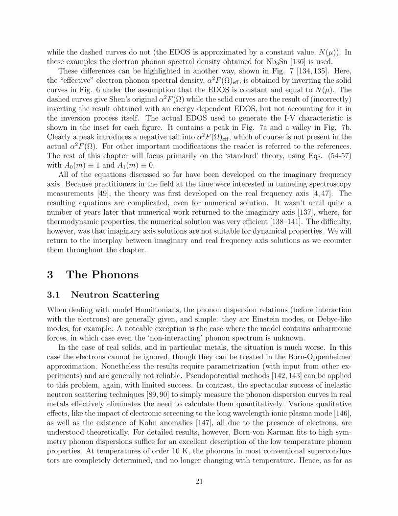


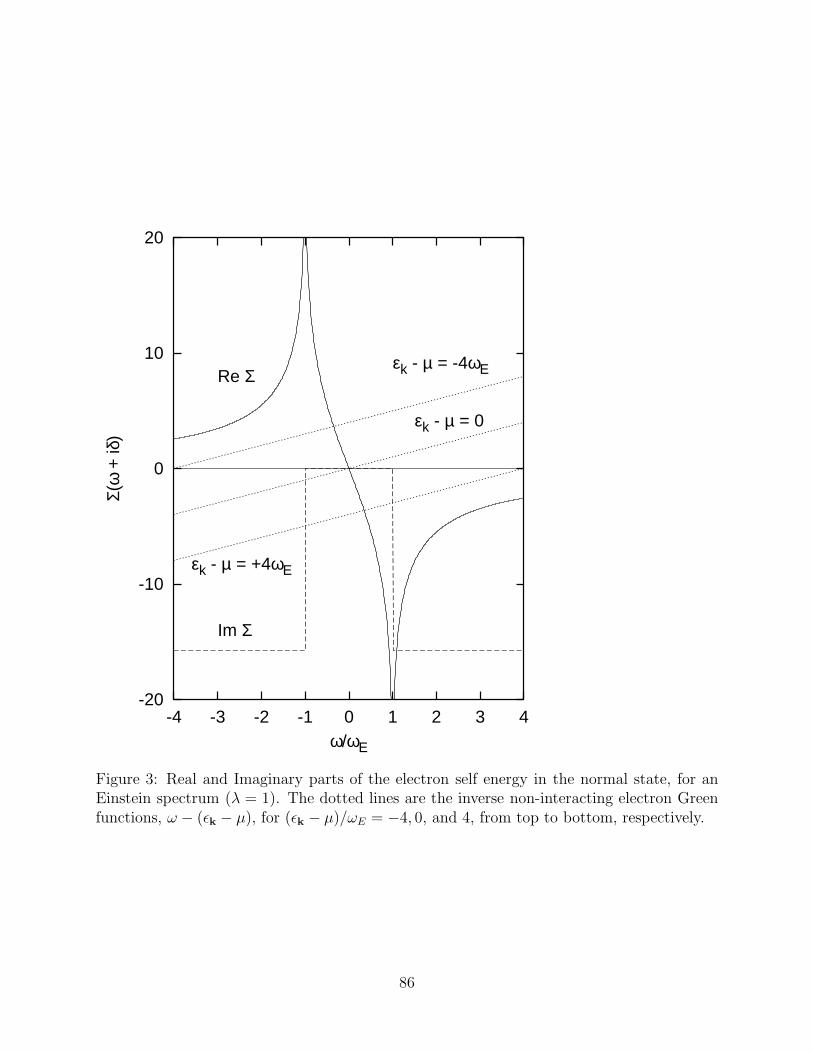


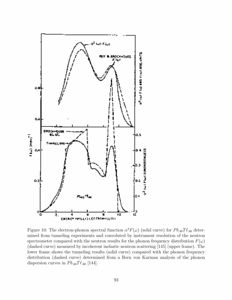
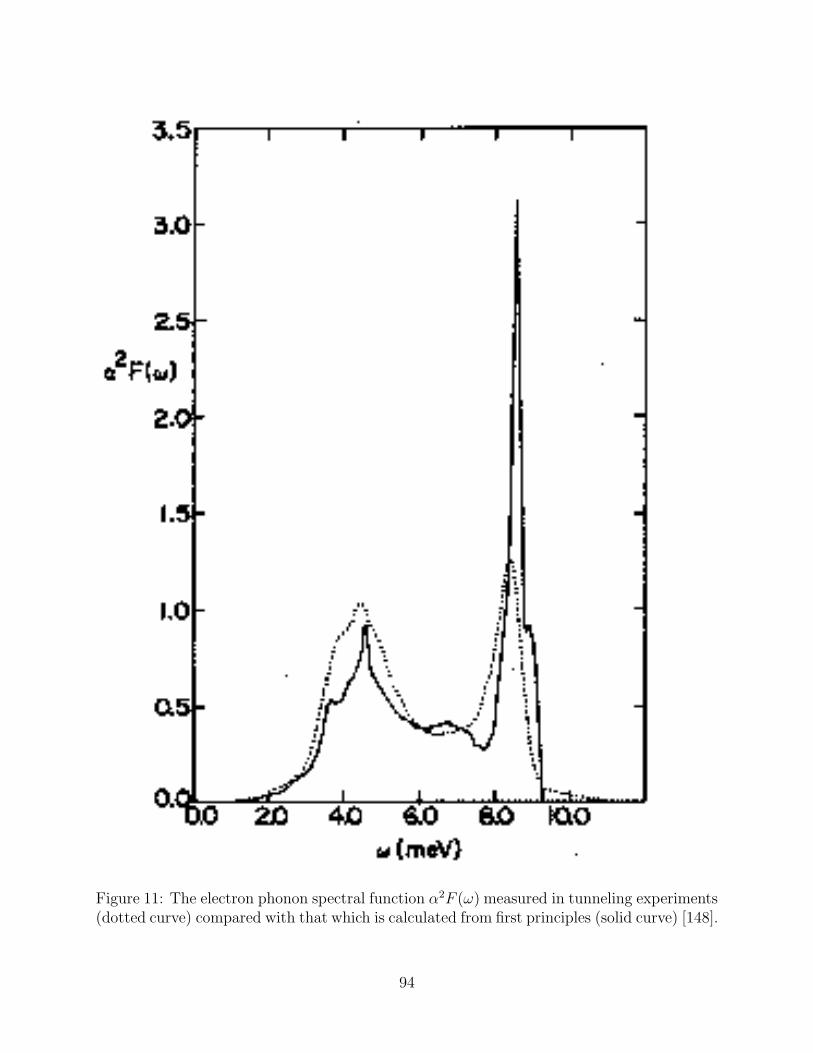
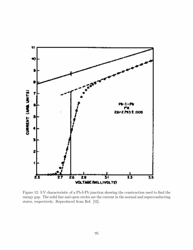


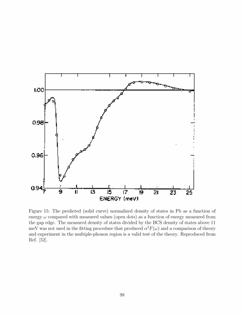


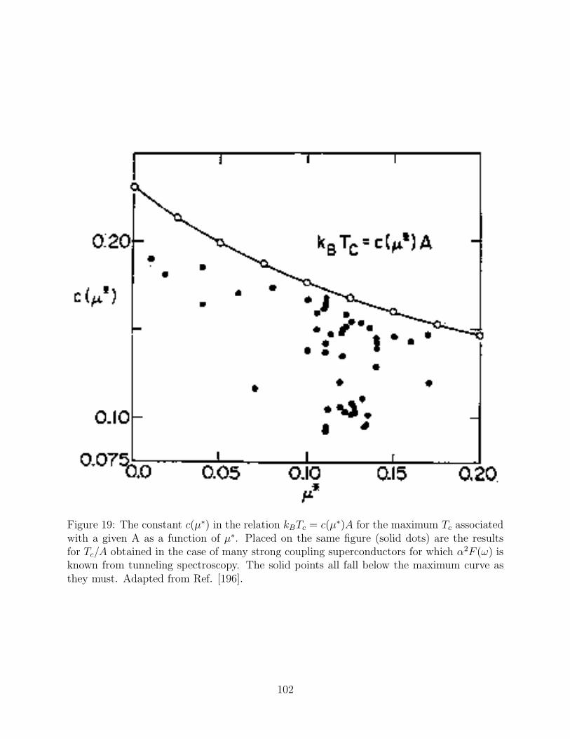
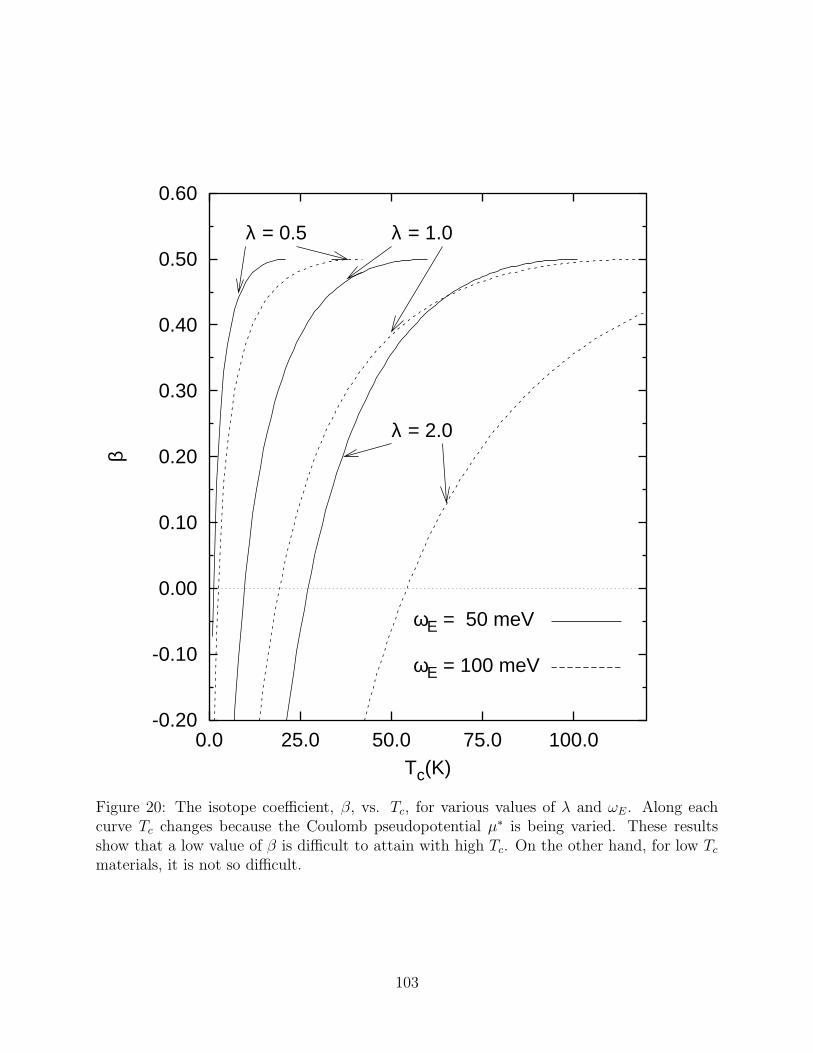
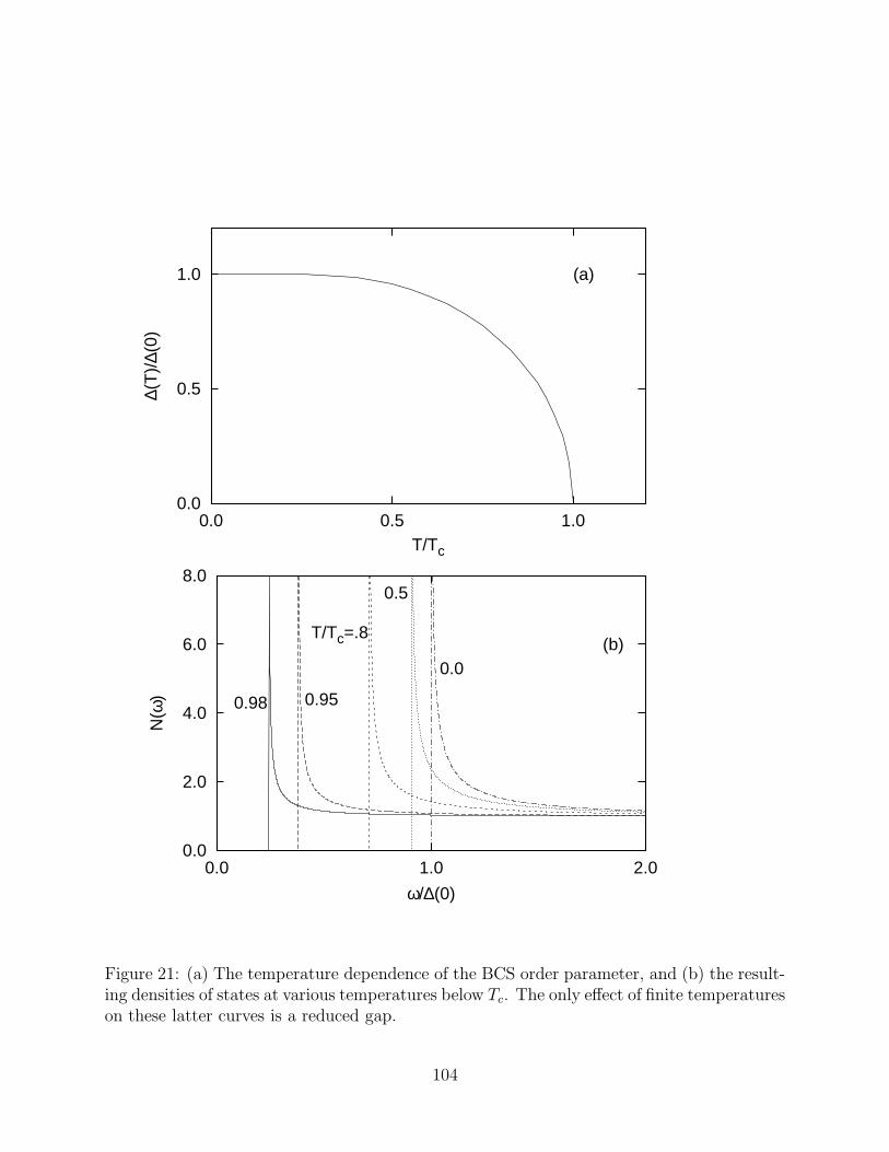

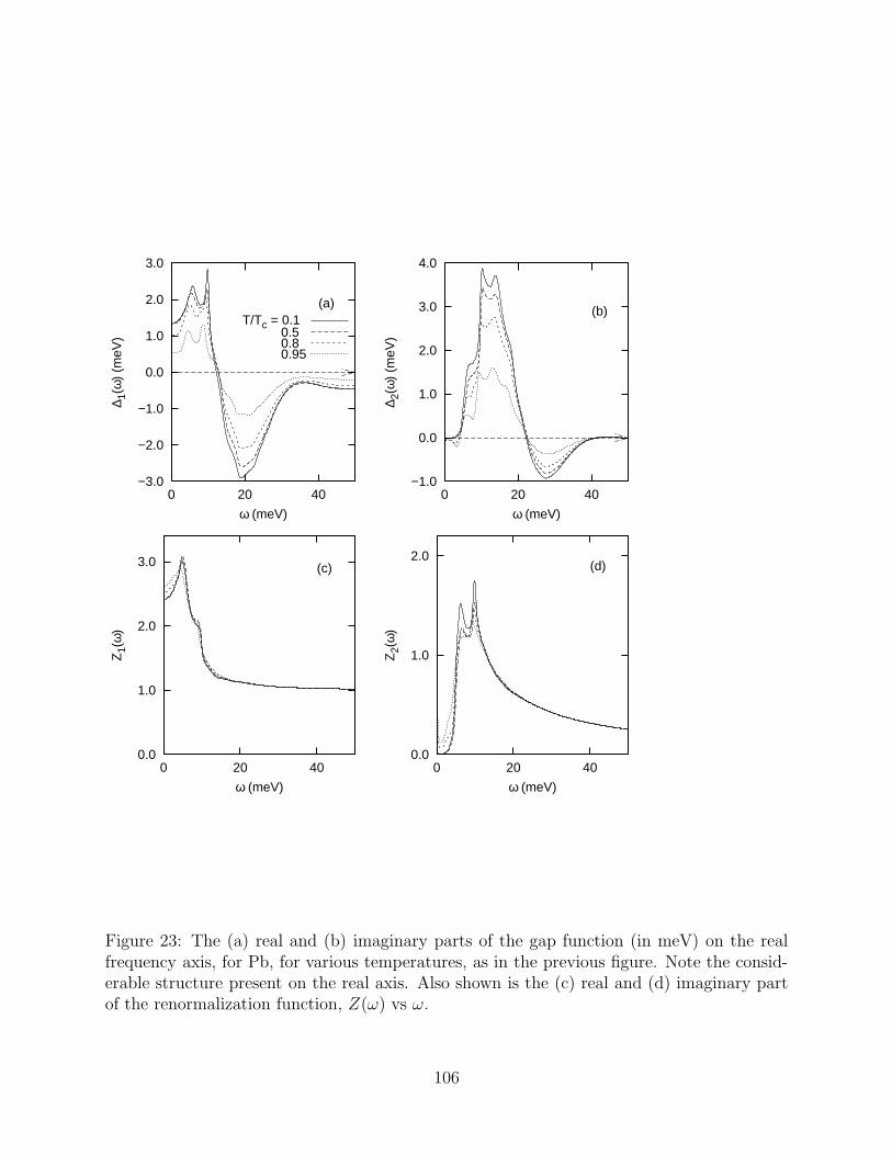
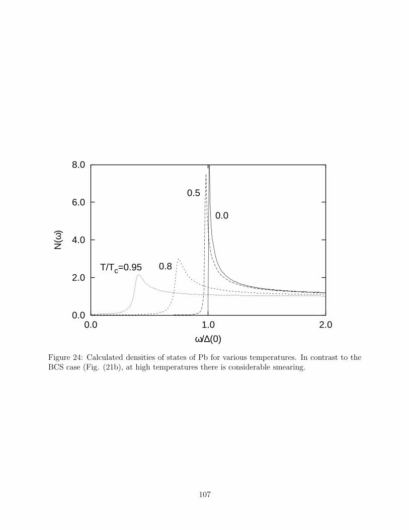

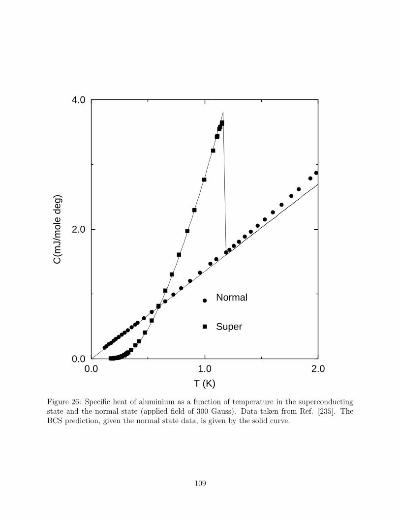


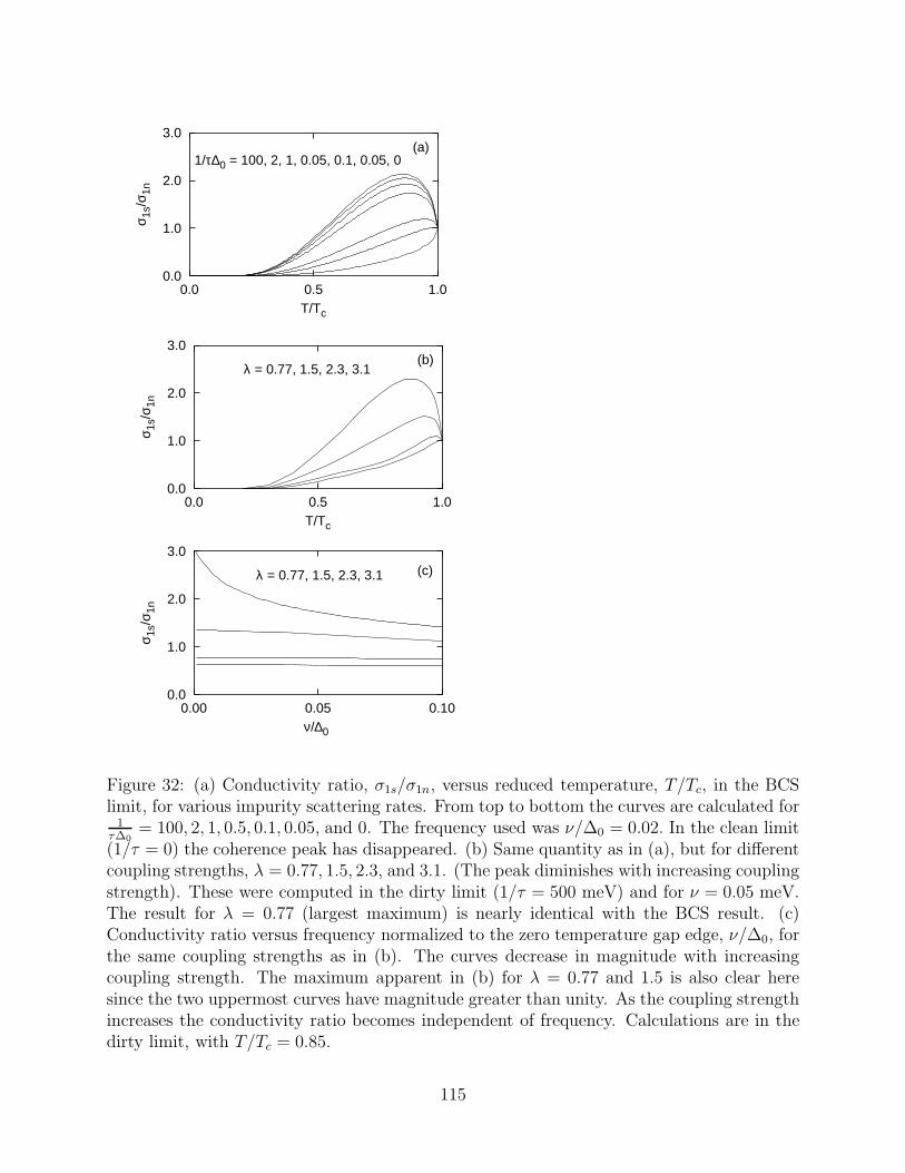


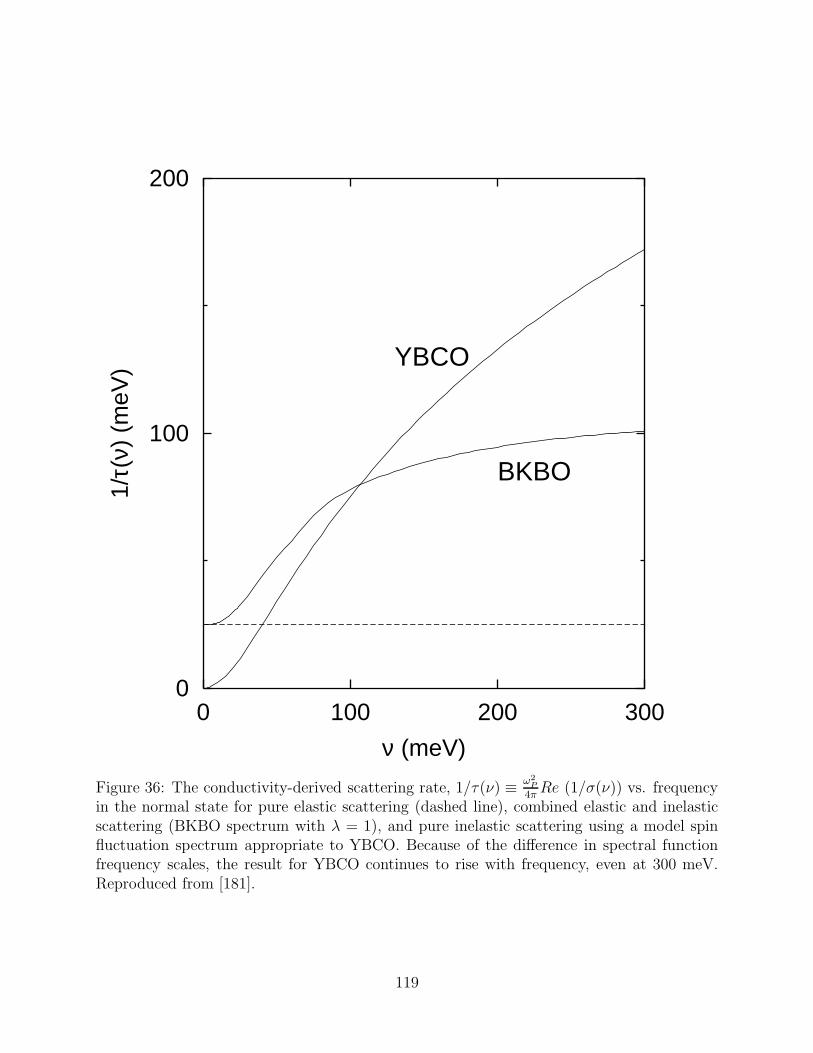

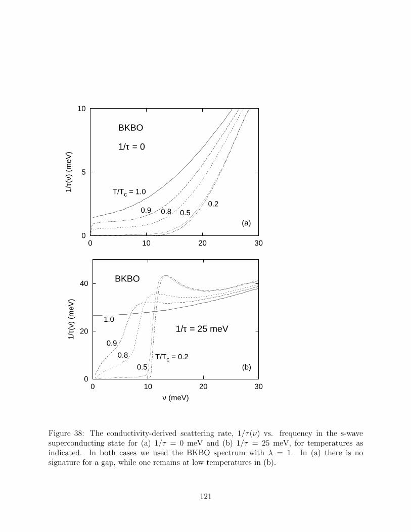


![arXiv:cond-mat/0106143v1 [cond-mat.supr-con] 7 …arXiv:cond-mat/0106143v1 [cond-mat.supr-con] 7 Jun 2001 Electron - Phonon Superconductivity F. Marsiglio and J.P. Carbotte February](https://static.documents.pub/doc/80x56/5ede2d68ad6a402d66697b08/arxivcond-mat0106143v1-cond-matsupr-con-7-arxivcond-mat0106143v1-cond-matsupr-con.jpg)


![Electron–Phonon Coupling in Two-Dimensional ...tion driven superconductivity in doped graphene [49] due to the very low electron– phonon coupling in graphene. Indeed, conventional](https://static.documents.pub/doc/80x56/613331aadfd10f4dd73aee43/electronaphonon-coupling-in-two-dimensional-tion-driven-superconductivity.jpg)


