57
3 May 2011 Olga Smirnova 1 MBI-Theory Electron recollision and High Harmonic Generation Tutorial Attofel summer school 3 May 2011, Crete Olga Smirnova Max-Born Institute
| Date post: | 05-Jun-2018 |
| Category: |
Documents |
| Upload: | trinhkhanh |
| View: | 214 times |
| Download: | 0 times |

3 May 2011Olga Smirnova
1MBI-Theory
Electron recollision and High Harmonic Generation
TutorialAttofel summer school 3 May 2011, Crete
Olga SmirnovaMax-Born Institute

3 May 2011Olga Smirnova
2MBI-Theory
HHG: How to generate them fast?
• S-matrix expression for HHG dipole (one electron)• Stationary phase method and factorization of the HHG
dipole (ionization, propagation, recombination)
• Stationary phase equations for HHG: The Lewenstein model
• The classical 3-step photoelectron model: where it goes wrong and how it can be improved
• HHG dipole for many electrons, including laser-induced dynamics in the ionic core between ionization and recombination

3 May 2011Olga Smirnova
3MBI-Theory
HHG: the non-linear optics perspective
HHG is frequency up-conversion. It results from macroscopic response of the medium:
2
2
22
2
22
2 41tP
ctE
czE
∂∂=
∂∂−
∂∂ π
The response is described by polarization P(t,z) induced in the medium:•response of atoms/molecules•response of free electrons•guiding medium (e.g. hollow core fiber)•etc
This lecture is about P(t) from individual atoms/molecules

3 May 2011Olga Smirnova
4MBI-Theory
HHG: the non-linear optics perspective
This lecture is about P(t) from individual atoms/molecules
n- number density)()( tnDtP =
),(ˆ),()( trdtrtD rr ΨΨ=
),()(),( trtHt
tri rr
Ψ=∂
Ψ∂
The key is to find the wavefunction
3 May 2011Olga Smirnova
5MBI-Theory
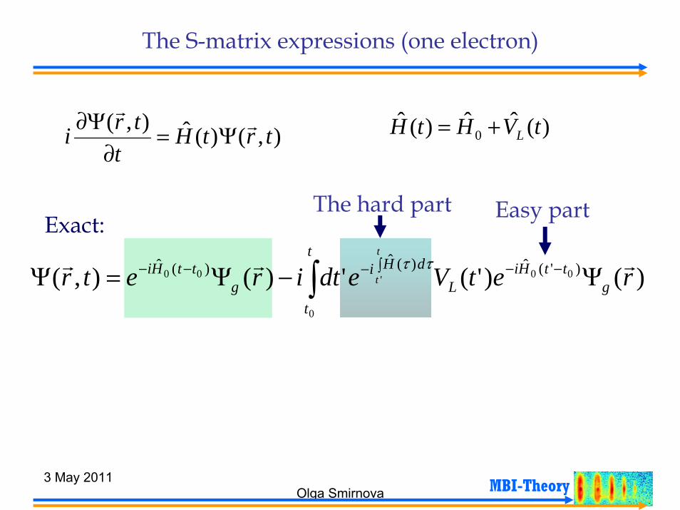
The S-matrix expressions (one electron)
),()(ˆ),( trtHt
tri rr
Ψ=∂
Ψ∂ )(ˆˆ)(ˆ0 tVHtH L+=
)()'(')(),( )'(ˆ)(ˆ)(ˆ00'
0
00 retVedtiretr gttHi
LdHi
t
tg
ttHit
trrr Ψ−Ψ=Ψ −−∫−−− ∫
ττ
Exact:The hard part Easy part

3 May 2011Olga Smirnova
6MBI-Theory
The S-matrix expressions (one electron)
),()(ˆ),( trtHt
tri rr
Ψ=∂
Ψ∂ )(ˆˆ)(ˆ0 tVHtH L+=
Neglect the Coulomb potentialThe SFA:
)()'(')(),( )'(ˆ)(ˆ)(ˆ 00'
0
00 retVedtiretr gttHi
LdHi
t
tg
ttHit
tLAS rrr Ψ−Ψ=Ψ −−∫−− ∫
ττ
Bound part Continuum part

3 May 2011Olga Smirnova
7MBI-Theory
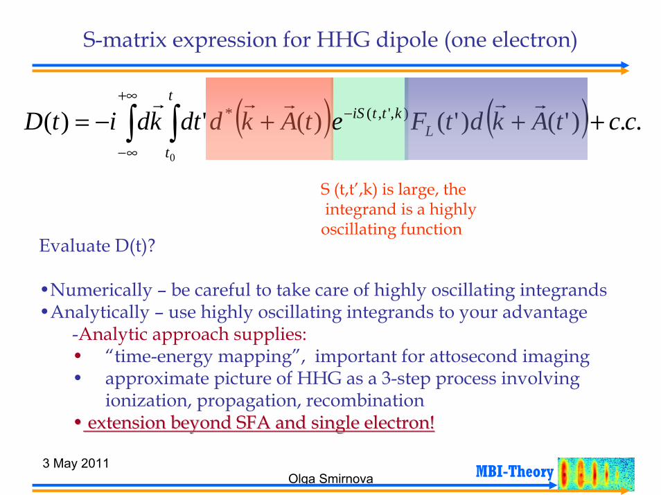
S-matrix expression for HHG dipole (one electron)
),(ˆ),()( trdtrtD rr ΨΨ=
..)()'('ˆ)()( )'(ˆ)(ˆ)(ˆ 00'
0
00 ccretVedtderitD gttHi
LdHi
t
t
ttHig
t
tLAS +ΨΨ−≈ −−∫−− ∫
rr ττ
Bound part Continuum part

3 May 2011Olga Smirnova
8MBI-Theory
S-matrix expression for HHG dipole (one electron)
),(ˆ),()( trdtrtD rr ΨΨ=
..)()'('ˆ)()( )'(ˆ)(ˆ)(ˆ 00'
0
00 ccretVedtderitD gttHi
LdHi
t
t
ttHig
t
tLAS +ΨΨ−≈ −−∫−− ∫
rr ττ
)'()'(1 tAktAkkdrrrrr
++= ∫+∞
∞−
Volkov functions, the length gauge:
)()'( '
2
'
)]([21
)(ˆtAketAke
t
t
t
tLAS
dAkidHirrrr
+=+∫ +−∫−
ττττ

3 May 2011Olga Smirnova
9MBI-Theory
S-matrix expression for HHG dipole (one electron)
( ) ( ))'()'()(' ),',(* tAkdtFetAkddt LkttiS ++ −
rrrr..)(
0
cckditDt
t
+−=+∞
∞−∫∫r
Phase (action)
( ) ( )∫ −++=t
tttIdAkkttS p
''2)(
21),',( ττ
rr
Ionization? Ionization? ––Not yet!Not yet!recombinationrecombination
Lewenstein et al, 1994
3 May 2011Olga Smirnova
10MBI-Theory
S-matrix expression for HHG dipole (one electron)
( ) ( ) ..)'()'()(')( ),',(*
0
cctAkdtFetAkddtkditD LkttiS
t
t
+++−= −+∞
∞−∫∫
rrrrr
Evaluate D(t)?
•Numerically – be careful to take care of highly oscillating integrands•Analytically – use highly oscillating integrands to your advantage
-Analytic approach supplies:• “time-energy mapping”, important for attosecond imaging • approximate picture of HHG as a 3-step process involving
ionization, propagation, recombination•• extension beyond SFA and single electron!
S (t,t’,k) is large, theintegrand is a highly oscillating function
extension beyond SFA and single electron!

3 May 2011Olga Smirnova
11MBI-Theory
Stationary phase method
e-iS(x)
Xx*)()( xSie
b
axfdx λ−
∫ 1>>λ
The integral is accumulated in points x*, where phase is stationary:
0*)(' =xSStationary phase region 1/√S’’ Idea:
2*)(*)(''*)*)(('*)()(
2xxxSxxxSxSxS −+−+=
2*)(*)(''*)(*)()()(
2xxxSiedxxSiexfxSie
b
axfdx
−−∫∞+
∞−
−≈−∫
λλλ
Can be evaluated analytically

3 May 2011Olga Smirnova
12MBI-Theory
(see Mathews, Walker,Mathematical Physics)Stationary phase method
e-iS(x)
Xx*)()( xSie
b
axfdx λ−
∫ 1>>λ
The integral is accumulated in points x*, where phase is stationary:
0*)(' =xSStationary phase region 1/√S’’ Idea:
2*)(*)(''*)*)(('*)()(
2xxxSxxxSxSxS −+−+=
( )[ ]*))(''(
4*)(
*)(*)(''
2)()( 1xSsignixSi
eOxfxS
xSieb
axfdx
πλλ
λπλ +−
+=−∫ −
)()( zSiezfdx λ
γ
−∫ For contour integrals in complex plane a
similar idea leads to the saddle point method

3 May 2011Olga Smirnova
13MBI-Theory
Saddle point method for HHG dipole
tiNkttiSt
t
eekddtdtND ωω ),',(
0
')( −+∞
∞−
+∞
∞−∫∫∫∝
rHarmonic spectrum:
Phase=S(t,t’,k)-Nω must be stationary wrt t,t’,k
( ) ( )∫ −++=t
tttIdAkkttS p
''2)(
21),',( ττ
rr
0'=
∂∂tS
0||
=∂∂kS 0=
∂∂
⊥kS
ωNtS =∂∂
1) Ionization time ti
Canonical momentum ks2)
Recombination time tr3)
If we know ti, tr, ks, we know D(Nω) Lewenstein et al, 1994
3 May 2011Olga Smirnova
14MBI-Theory
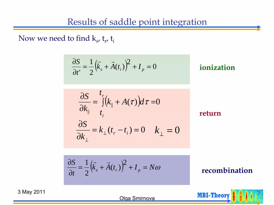
Results of saddle point integration
Now we need to find ks, tr, ti
( ) 02)(21
'=++=
∂∂
pis ItAktS rr
ionization
( ) 0)(||||
∫ =+=∂∂ r
i
t
tdAk
kS ττ
0)( =−=∂∂
⊥⊥
ir ttkkS 0=⊥k
return
( ) ωNItAktS
prs =++=∂∂ 2)(
21 rr
recombination

3 May 2011Olga Smirnova
15MBI-Theory
Complex ionization time
( ) 02)(21 =++ pis ItAk Ionization time ti is complex ti= ti’+i ti’’1)
Real time
Imaginary time
ti
Tunnel entrance
Tunnel entrance ti=ti’+ti’’
t
Tunnel exit
Tunnel exit
( ) exexist
ex izzitAkdizi
''')'(0
''
+=++= ∫ ττ
ti’’
ti’
t’i
The coordinate at the exit is complex
3 May 2011Olga Smirnova
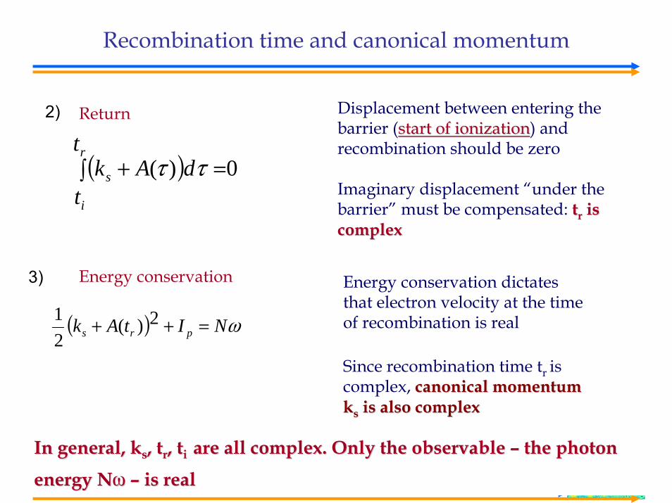
16MBI-Theory
Recombination time and canonical momentum
Displacement between entering the barrier (start of ionizationstart of ionization) and recombination should be zero
Imaginary displacement “under the barrier” must be compensated: ttrr is is complex
2) Return
( ) 0)(∫ =+r
i
s
t
tdAk ττ
complex
3) Energy conservation Energy conservation dictates that electron velocity at the time of recombination is real( ) ωNItAk prs =++ 2)(
21
Since recombination time tr is complex, canonical momentum canonical momentum kkss is also complexis also complex
In general, In general, kkss, , ttrr, , ttii are all complex. Only the observable are all complex. Only the observable –– the photon the photon
energy energy NNωω –– is realis real

3 May 2011Olga Smirnova
17MBI-Theory
Quantum orbits (Salieres et al, 2000)
How to solve 3 saddle point equations? Total 6 unknowns: ti’,ti’’, tr’,tr’’, ks’,ks’’
( ) 0)(∫ =+r
i
s
t
tdAk ττ( ) 02)(
21 =++ pis ItAk
rr( ) ωNItAk prs =++ 2)(
21
Total 6 equations: for real and imaginary parts. Goal: Set N Find ti’,ti’’, tr’,tr’’, ks’,ks’’
All 6 All 6 eqseqs. do not have analytical solutions. . do not have analytical solutions.
Step 1: express everything via return time (imaginary and real),Step 1: express everything via return time (imaginary and real), using 4 using 4 eqseqs..Step 2: solve the remaining 2 equations togetherStep 2: solve the remaining 2 equations together
3 May 2011Olga Smirnova
18MBI-Theory
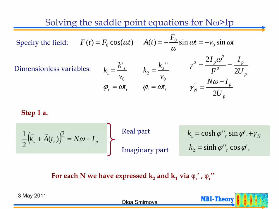
Solving the saddle point equations for Nω>Ip
tvtFtA ωωω
sinsin)( 00 −=−=)cos()( 0 tFtF ω=Specify the field:
p
pp
UI
FI
22
2
22 ==
ωγ
02
''vkk s=
ii tωϕ =0
1'
vkk s=Dimensionless variables:
p
pN U
IN2
2 −=
ωγrr tωϕ =
Step 1 a.Step 1 a.
( ) prs INtAk −=+ ω2)(21 rr Real part
rrk 'cos''sinh2 ϕϕ=Nrrk γϕϕ += 'sin''cosh1
Imaginary part
For each N we have expressed k2 and k1 via ϕr’ , ϕr’’

3 May 2011Olga Smirnova
19MBI-Theory
Solutions of the saddle point equationsStep 1 b.Step 1 b.
1''cosh'sin kii =ϕϕ
2'cos''sinh kii += γϕϕ
Real part
Imaginary part( ) 02)(
21 =++ pis ItAk
2~ k+= γγ1~22
1 ++= γkP2
12 4kPD −=
( ) )2/arcsin(' DPi +=ϕ
( ) )2/arccosh('' DPi −=ϕ
For each N we have expressed k2 and k1 via ϕr’ , ϕr’’ and we have expressed ϕi’ , ϕi’’via k1, k2
Hence ϕi’ , ϕi’’ and k1, k2 are all expressed via ϕr’ , ϕr’’
Now we can use the remaining equations to find ϕr’ , ϕr’’

3 May 2011Olga Smirnova
20MBI-Theory
Solutions of the saddle point equations
( ) 0)(∫ =+r
i
s
t
tdAk ττStep 2: Now use the last equation:
( ) ( ) 0'cos''cosh''cosh'cos'''''' 211 =+−−−−= rriiirir kkF ϕϕϕϕϕϕϕϕReal part
( ) ( ) 0'sin''sinh''sinh'sin'''''' 212 =−+−+−= rriiirir kkF ϕϕϕϕϕϕϕϕIm part
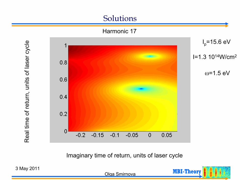
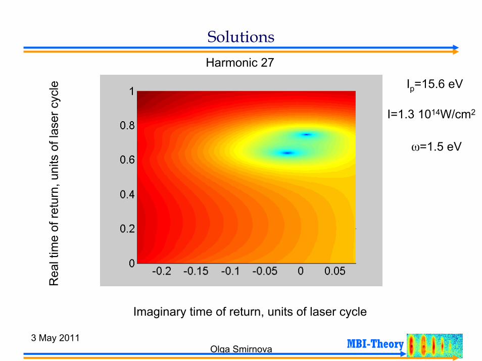
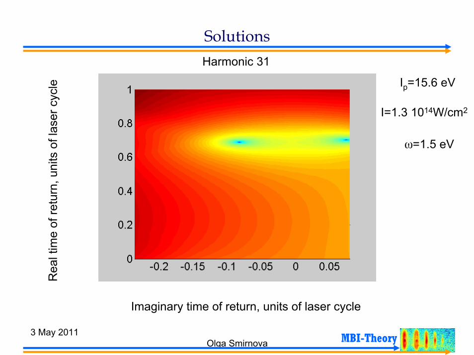
( )[ ] ( )[ ] 0'',','',', 22
21 =+ rrrr NFNF ϕϕϕϕ
Set grid of ϕr’ and ϕr’’ and numerically find minimum of this surface for each N

3 May 2011Olga Smirnova
21MBI-Theory
SolutionsHarmonic 11
Ip=15.6 eV
Rea
l tim
e of
retu
rn, u
nits
of l
aser
cyc
le
I=1.3 1014W/cm2
ω=1.5 eV
Imaginary time of return, units of laser cycle

3 May 2011Olga Smirnova
22MBI-Theory
SolutionsHarmonic 13
Ip=15.6 eV
Rea
l tim
e of
retu
rn, u
nits
of l
aser
cyc
le
I=1.3 1014W/cm2
ω=1.5 eV
Imaginary time of return, units of laser cycle

3 May 2011Olga Smirnova
23MBI-Theory
SolutionsHarmonic 15
Ip=15.6 eV
Rea
l tim
e of
retu
rn, u
nits
of l
aser
cyc
le
I=1.3 1014W/cm2
ω=1.5 eV
Imaginary time of return, units of laser cycle
3 May 2011Olga Smirnova
24MBI-Theory
SolutionsHarmonic 17
Ip=15.6 eV
Rea
l tim
e of
retu
rn, u
nits
of l
aser
cyc
le
I=1.3 1014W/cm2
ω=1.5 eV
Imaginary time of return, units of laser cycle

3 May 2011Olga Smirnova
25MBI-Theory
SolutionsHarmonic 19
Ip=15.6 eV
Rea
l tim
e of
retu
rn, u
nits
of l
aser
cyc
le
I=1.3 1014W/cm2
ω=1.5 eV
Imaginary time of return, units of laser cycle

3 May 2011Olga Smirnova
26MBI-Theory
SolutionsHarmonic 21
Ip=15.6 eV
Rea
l tim
e of
retu
rn, u
nits
of l
aser
cyc
le
I=1.3 1014W/cm2
ω=1.5 eV
Imaginary time of return, units of laser cycle

3 May 2011Olga Smirnova
27MBI-Theory
SolutionsHarmonic 23
Ip=15.6 eV
Rea
l tim
e of
retu
rn, u
nits
of l
aser
cyc
le
I=1.3 1014W/cm2
ω=1.5 eV
Imaginary time of return, units of laser cycle

3 May 2011Olga Smirnova
28MBI-Theory
SolutionsHarmonic 25
Ip=15.6 eV
Rea
l tim
e of
retu
rn, u
nits
of l
aser
cyc
le
I=1.3 1014W/cm2
ω=1.5 eV
Imaginary time of return, units of laser cycle
3 May 2011Olga Smirnova
29MBI-Theory
SolutionsHarmonic 27
Ip=15.6 eV
Rea
l tim
e of
retu
rn, u
nits
of l
aser
cyc
le
I=1.3 1014W/cm2
ω=1.5 eV
Imaginary time of return, units of laser cycle

3 May 2011Olga Smirnova
30MBI-Theory
SolutionsHarmonic 29
Ip=15.6 eV
Rea
l tim
e of
retu
rn, u
nits
of l
aser
cyc
le
I=1.3 1014W/cm2
ω=1.5 eV
Imaginary time of return, units of laser cycle
3 May 2011Olga Smirnova
31MBI-Theory
SolutionsHarmonic 31
Ip=15.6 eV
Rea
l tim
e of
retu
rn, u
nits
of l
aser
cyc
le
I=1.3 1014W/cm2
ω=1.5 eV
Imaginary time of return, units of laser cycle

3 May 2011Olga Smirnova
32MBI-Theory
Energy of return
Short and long trajectories: two different saddle point solutions for the same Energy of return (Harmonic number)
Cut-off
short longtrajectories
Below threshold harmonics
Saddle point method breaks down near the cut-off: 2 saddle points merge (Stt’’=0)

3 May 2011Olga Smirnova
33MBI-Theory
Imaginary time of return
Imaginary& real time of return define integration contour in complex plane: only along this contour the energy of return is real.
Cut-off
Belowthreshold Short Long
Difficult part is here: divergence

3 May 2011Olga Smirnova
34MBI-Theory
Imaginary time of return
Imaginary& real time of return define integration contour in complex plane: only along this contour the energy of return is real.
Cut-off
Belowthreshold Short Long
Would be niceto have it like so

3 May 2011Olga Smirnova
35MBI-Theory
Treating the cut-off regionStep1: Step1: Find tr =t0 (and ti=ti0, ks=ks0), such that Stt’’ (tr0,ti0,ks0) =0, i.e. dEret/dt=0(Pick the cut-off (real) return time for t0)
Step2:Step2:Expand the action S(tr,ti,ks) around t0 ( the uniform approximation( the uniform approximation )
6)(),,())(,,(),,(),,(
30
000'''
0000'
00000ttkttSttkttSkttSkttS iitttiitiiii
−+−+=
Step3:Step3:
The resulting integral for dipole: ..)( ),,( 00 cceedtND tiNkttiS si +∝ −+∞
∞−∫ ωω
can be calculated analytically using Airy function:
( ) ( ) ⎥⎦
⎤⎢⎣
⎡±≡±∫
+∞
∞−3/13/1
3
33)cos(
axAi
axtat π

3 May 2011Olga Smirnova
36MBI-Theory
Treating the cut-off region
Introduce the cut-off harmonic number NN0 0 and “the distance from cut-off” ∆∆N=NN=N-- NN00 :
(N0 does not have to be integer )ω000' )()( NItEtS prett ≡+=
The dipole near cut-off is expressed via Airy function :
ξωξξχω ω dNcceedtND tiNkttiS si )6
cos(..)( 3),,( 00 ∆+=+∝ ∫∫+∞
∞−
−+∞
∞−
[ ] ( ) ⎥⎦
⎤⎢⎣
⎡ ∆∝ 3131 222)(
χω
χπω NAiND
∆N<0 before cut-off: Ai~cos[-(∆Nω)3/2 (8/9χ)1/2 ]
∆N>0 after cut-off: Ai~exp[-(∆Nω)3/2 (8/9χ)1/2 ]
(oscillations are due to interference of short and long)
(exponential decrease of HH spectrum after cut-off)ωχ 00 )( Ftv≅ ω00' )( FtFt ≅
0)( 0 ≅tF
)( 0''' tSttt−=χ

3 May 2011Olga Smirnova
37MBI-Theory
Ionization times: sub-cycle dynamics of ionizationBelowthreshold Short Long
Ionization window
time
~250asec
670asec
0 1
Imaginary ionization time defines ionization probability:short trajectories are suppressedReal ionization time defines “duration of ionization window”

3 May 2011Olga Smirnova
38MBI-Theory
Canonical momenta
Belowthreshold
Short Long
Belowthreshold
Short Long
Long trajectories: imaginary canonical momentum is very smallShort trajectories: substantial imaginary canonical momentumPhotoelectrons: registered at the detector - canonical momentum is real

3 May 2011Olga Smirnova
39MBI-Theory
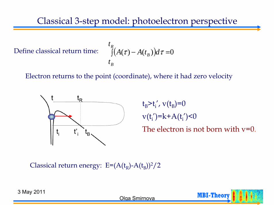
Classical 3-step model: photoelectron perspective
Define “classical ionization time” – “time of birth”, when electron velocity is zero.
( ) 02)()(21 =+− pBi ItAtAv(tB)=k+A(tB)=0 v(ti)=A(ti)-A(tB)=-i γ
k=-A(tB) Different from “quantum ionization times”, since k is forced to be real.
Real time
Imaginary time
Tunnel entrance ti=ti’+ti’’
Tunnel exit
t
ti’’
ti’ tB
v=0
Imaginary ionization time
Real ionization time
3 May 2011Olga Smirnova
40MBI-Theory
Classical 3-step model: photoelectron perspective
( ) 0)()(∫ =−R
B
B
t
tdtAA ττDefine classical return time:
Electron returns to the point (coordinate), where it had zero velocity
ti t’i tB
tB>ti’, v(tB)=0v(ti’)=k+A(ti’)<0
The electron is not born with v=0.
Classical return energy: E=(A(tR)-A(tB))2/2

3 May 2011Olga Smirnova
41MBI-Theory
Classical energy of returnClassical cut-off corresponds to lower energies:electron does not return to the core
Cut-off: 3.17 Up+1.32 Ip
short longtrajectories
Below threshold harmonics
Cut-off: 3.17 Up+ Ip
Can we improve these results? Let’s let the photo-electrons return to the core.

3 May 2011Olga Smirnova
42MBI-Theory
Photoelectrons vs Lewenstein modelEnergy at closest approach: not all electrons can return exactly to the core since we limited k=-A(tB)
Belowthreshold:n/a
Short Long
Lewenstein model
Improved 3 Improved 3 ––step model (k<1) +step model (k<1) +relaxed return condition:relaxed return condition:
•Neglect Imag ∆z =0 •Minimize Real ∆z
The strict requirement of perfect return is an artefact of neglecting the size of the ground state. Relaxing this requirement seems quite reasonable!

3 May 2011Olga Smirnova
43MBI-Theory
Photoelectrons: return coordinate
Not all electrons can return exactly to the core since we limited k=-A(tB)
Return is notpossible(with k<1)
Exactreturn on real axis Re
al ∆
z
Real time of return, units of laser cycle

3 May 2011Olga Smirnova
44MBI-Theory
Photoelectrons: saddle point region
Real k should be within the saddle point region of the exact complex saddle point. This region is ~ |S’’kk|-1/2
Inside the stationary phase region
|∆k|<|tr-ti|1/2
|∆k|=∆z/(tr-ti)
|∆k|<|S’’kk|-1/2
|∆z|<(tr-ti) 1/2
Real time of return, units of laser cycle
|∆k|- difference between the exact ks and photolelctron ks|∆z|- distance of the closest approach to the core
|∆z|<(tr-ti) 1/2
(tr-ti) 1/2
|∆z|
3 May 2011Olga Smirnova
45MBI-Theory
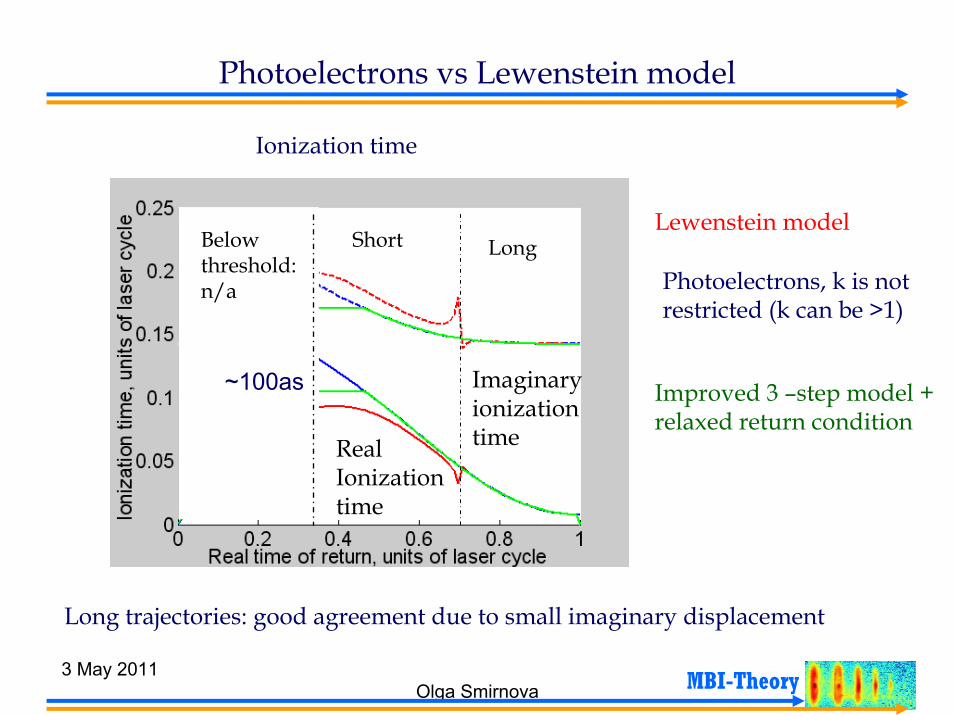
Photoelectrons vs Lewenstein model
Ionization time
Belowthreshold:n/a
Short Long
ImaginaryionizationtimeReal
Ionizationtime
~100as
Lewenstein model
Photoelectrons, k is not restricted (k can be >1)
Improved 3 –step model +relaxed return condition
Long trajectories: good agreement due to small imaginary displacement
3 May 2011Olga Smirnova
46MBI-Theory
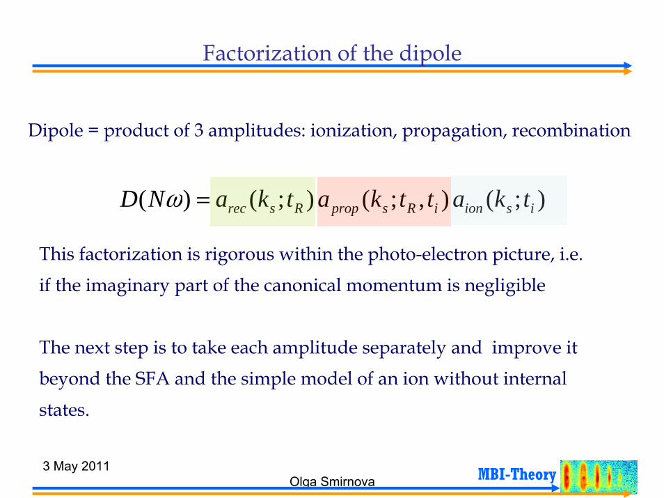
Factorization of the dipole
Dipole = product of 3 amplitudes: ionization, propagation, recombination
);(),;();()( isioniRspropRsrec tkattkatkaND =ω
This factorization is rigorous within the photo-electron picture, i.e. if the imaginary part of the canonical momentum is negligible
The next step is to take each amplitude separately and improve it beyond the SFA and the simple model of an ion without internal
states.

3 May 2011Olga Smirnova
47MBI-Theory
Results of saddle point integration
Dipole = product of 3 amplitudes: ionization, propagation, recombination
);(),;();()( isioniRspropRsrec tkattkatkaND =ω
( ) ( )
'',
')(21
'2
)]([~);(ii
it
itiips
tt
ttiIdAki
issionS
etAkdtka πττ∫ −−+−
+rr
The amplitudes are (within saddle point): 1. Ionization
Re time
Im timeti=Re[ti]+ i*Im[ti ]=ti’+ i ti’’

3 May 2011Olga Smirnova
48MBI-Theory
Results of saddle point integration
Dipole = product of 3 amplitudes: ionization, propagation, recombination
);(),;();()( isioniRspropRsrec tkattkatkaND =ω
The amplitudes are (within saddle point):
Propagation: wavepacket spreading and phase accumulation
( ) ( )
2/3
3')(21
][~)';;( '
2
iR
ttiIdAki
iRsprop ttettka
Rt
itiRps
−
∫ −−+− πττrr

3 May 2011Olga Smirnova
49MBI-Theory
Results of saddle point integration
Dipole = product of 3 amplitudes: ionization, propagation, recombination
);()',;();()( isioniRspropRsrec tkattkatkaND =ω
The amplitudes are (within saddle point):
Recombination: proportional to the recombination dipole
''))((*~);(
RRtt
RsRsrecS
tAkdtka π+
3 May 2011Olga Smirnova
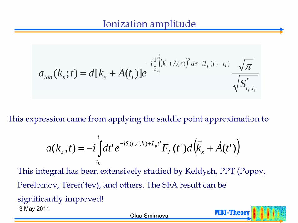
50MBI-Theory
Ionization amplitude
( ) ( )
'',
')(21
'2
)]([);(ii
it
itiips
tt
ttiIdAki
issionS
etAkdtka πττ∫ −−+−
+=rr
This expression came from applying the saddle point approximation to
( ))'()'('),( '),',(
0
tAkdtFedtitka sLtIkttiS
t
ts
prr
+−= +−∫This integral has been extensively studied by Keldysh, PPT (Popov, Perelomov, Teren’tev), and others. The SFA result can be
significantly improved!

3 May 2011Olga Smirnova
51MBI-Theory
Ionization amplitude
),(tSFAexponen, ),(),( is tk
pmlision eFIRtka −=
The recipe for atoms: (PPT, Keldysh, Yudin-Ivanov, Becker-Faisal, Popruzhenko-Bauer) SubSub--cycle ratescycle rates
-Calculate exponential dependence with SFA- Add Coulomb correction Rlm to account for the core.
- The Coulomb correction depends on l, m - With reasonable accuracy and for linearly polarized or low-
frequency fields the Coulomb correction can be taken from statictunneling The recipe for molecules: Take the Coulomb correction from static
tunneling rates (MO-ADK (Tong&Lin), recently Murray & Ivanov)

3 May 2011Olga Smirnova
52MBI-Theory
The Multi-Channel Case
Exact ‘continuum’ part: electron+ion
gttHi
LdHi
t
tc etVedtit
t
t Ψ−=Ψ −−∫−∫)'(ˆ)(ˆ
00'
0
)'(')( ττ
)'()'(1 tAknntAkkdn
rrrrr++= ∫∑
+∞
∞− Polarized Core states
Continuum states
gttHi
LdHi
t
tnc etVtknntkedtkdit
t
t Ψ−=Ψ −−∫−+∞
∞−∫∫∑ )'(ˆ)(ˆ
00'
0
)'()'()'(')(rrr ττ
nD
ttHiL etVtk Ψ−− )'(ˆ
00)'()'(r
gnD n Ψ∝ΨDyson orbital:

3 May 2011Olga Smirnova
53MBI-Theory
The Multi-Channel Case
Exact ‘continuum’ part: electron+ion
gttHi
LdHi
t
tc etVedtit
t
t Ψ−=Ψ −−∫−∫)'(ˆ)(ˆ
00'
0
)'(')( ττ
)'()'(1 tAknntAkkdn
rrrrr++= ∫∑
+∞
∞− Polarized Core states
Continuum states
nD
ttHiL
dHit
tnc etVtkntkedtkdit
t
t Ψ−=Ψ −−∫−+∞
∞−∫∫∑ )'(ˆ)(ˆ
00'
0
)'()'()'(')(rrr ττ
Neglect e-e correlation after ionization: the continuum electron moves in a self-consistent field of the core

3 May 2011Olga Smirnova
54MBI-Theory
The Multi-Channel Case
Exact ‘continuum’ part: electron+ion
nD
ttHiL
dHit
tnc etVtkntkedtkdit
t
t Ψ−=Ψ −−∫−+∞
∞−∫∫∑ )'(ˆ)(ˆ
00'
0
)'()'()'(')(rrr ττ
Neglect e-e correlation after ionization: the continuum electron moves in a self-consistent field of the core
nD
ttHiL
dHidHit
tnc etVtknetkedtkdit
t
ti
t
tc Ψ−=Ψ −−∫−∫−
+∞
∞−∫∫∑ )'(ˆ)(ˆ)(ˆ
00''
0
)'()'()'(')(rrr ττττ
continuum ion
Evolution in the continuum – like beforeEvolution in the ion – start in |n> at t’, end in |m> at t, amplitude amn(t,t’)

3 May 2011Olga Smirnova
55MBI-Theory
The Multi-Channel Case
nD
ttHiL
dHidHit
tnc etVtknetkedtkdit
t
ti
t
tc Ψ−=Ψ −−∫−∫−
+∞
∞−∫∫∑ )'(ˆ)(ˆ)(ˆ
00''
0
)'()'()'(')(rrr ττττ
continuum ion
Ion |n>
Ion |m>-
ionization
recombination

3 May 2011Olga Smirnova
56MBI-Theory
The harmonic dipole in the multi-channel case
The harmonic dipole is a sum over all ionic states at tion and trec
);(),;();()( ,,,,
isnioniRsmnpropRsmrecmn
tkattkatkaND ∑=ω
The key change is in the propagation amplitude— it includes transitions between the initial (n) and the final (m) states of the ionic core:
Recombination –the electron recombines with the ion in the state m:
( ) ( )
2/3
3')(21
,, ][)',(~)';;( '
,2
iR
ttiIdAki
iRmncoreiRsmnprop ttettattka
Rt
itiRnps
−
∫ −−+− πττrr
'', ))((*~);(RRtt
RsmRsmrec StAkdtka π+

3 May 2011Olga Smirnova
57MBI-Theory
Example of core dynamics in the multi-channel case
Populations of ionic states
X 2Σ+g
A 2Πu
B 2Σ+u
0 0.25 0.5 0.75 10
0.2
0.4
0.6
0.8
1
|A|2
|X|2
|B|2
3.5eV1.3 eV
Ip~15.6 eV
Time, laser cycleInitial condition: population of the polarized ground state of N2
+ upon ionization, I=1014W/cm2
Find dipole couplings between the states A,B,X. Solve 3-level system numerically


![i .] APPROXIMATING HARMONIC FUNCTIONS 499€¦ · APPROXIMATING HARMONIC FUNCTIONS 499 THE APPROXIMATION OF HARMONIC FUNCTIONS BY HARMONIC POLYNOMIALS AND BY HARMONIC RATIONAL FUNCTIONS*](https://static.documents.pub/doc/80x56/5f0873ba7e708231d42214c2/i-approximating-harmonic-functions-499-approximating-harmonic-functions-499-the.jpg)