Electron Spin Resonance - Факультет Естественных...

Electron Spin Resonance

by

Dr. Phil Rieger Brown University

ESR Spectroscopy 2

© Copyright Dr. Phil Rieger, Brown University

Electron Spin Resonance

1. Introduction

Electron spin resonance (ESR) spectroscopy has been used for over 50 years to study a variety of paramagnetic species. In this chapter, we will focus on the spectra of organic and organotransition metal radicals and coordination complexes. Although ESR spectroscopy is supposed to be a mature field with a fully developed theory [1], there have been some surprises as organometallic problems have explored new domains in ESR parameter space. We will start with a synopsis of the fundamentals of ESR spectroscopy. For further details on the theory and practice of ESR spectroscopy, refer to one of the excellent texts on ESR spectroscopy [2-9].

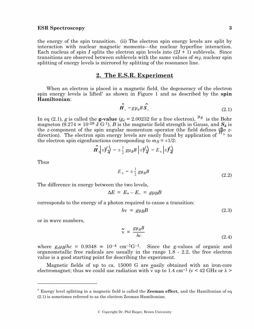
The electron spin resonance spectrum of a free radical or coordination complex with one unpaired electron is the simplest of all forms of spectroscopy. The degeneracy of the electron spin states characterized by the quantum number, mS = ±1/2, is lifted by the application of a magnetic field and transitions between the spin levels are induced by radiation of the appropriate frequency, as shown in Figure 1.1. If unpaired electrons in radicals were indistinguishable from free electrons, the only information content of an ESR spectrum would be the integrated intensity, proportional to the radical con-centration. Fortunately, an un-

-0.3

-0.2

-0.1

0

0.1

0.2

0.3 E /cm -1

0 1000 2000 3000 4000 5000B /Gauss

Figure 1.1. Energy levels of an electron placed in a magnetic field. The arrow shows the transitions induced by 0.315 cm-1 radiation.

paired electron interacts with its environment, and the details of ESR spectra depend on the nature of those interactions.

There are two kinds of environmental interactions which are commonly important in the ESR spectrum of a free radical: (i) To the extent that the unpaired electron has unquenched orbital angular momentum, the total magnetic moment is different from the spin-only moment (either larger or smaller, depending on how the angular momentum vectors couple). It is customary to lump the orbital and spin angular momenta together in an effective spin and to treat the effect as a shift in

ESR Spectroscopy 3


the energy of the spin transition. (ii) The electron spin energy levels are split by interaction with nuclear magnetic moments—the nuclear hyperfine interaction. Each nucleus of spin I splits the electron spin levels into (2I + 1) sublevels. Since transitions are observed between sublevels with the same values of mI, nuclear spin splitting of energy levels is mirrored by splitting of the resonance line.

2. The E.S.R. Experiment

When an electron is placed in a magnetic field, the degeneracy of the electron spin energy levels is lifted* as shown in Figure 1 and as described by the spin Hamiltonian:

H s = gµBB S z (2.1)

In eq (2.1), g is called the g-value (ge = 2.00232 for a free electron), µB is the Bohr

magneton (9.274 ∞ 10-28 J G-1), B is the magnetic field strength in Gauss, and Sz is the z-component of the spin angular momentum operator (the field defines the z-direction). The electron spin energy levels are easily found by application of

H s to the electron spin eigenfunctions corresponding to mS = ±1/2:

H s ±1 21 2 = ± 1

2gµBB ±1 21 2 = E ± ±1 21 2

Thus

E ± = ± 1

2gµBB

(2.2)

The difference in energy between the two levels,

∆E = E+ – E– = gµBB

corresponds to the energy of a photon required to cause a transition:

hν = gµBB (2.3)

or in wave numbers,

ν =

gµBBhc (2.4)

where geµB/hc = 0.9348 ∞ 10–4 cm–1G–1. Since the g-values of organic and organometallic free radicals are usually in the range 1.8 - 2.2, the free electron value is a good starting point for describing the experiment.

Magnetic fields of up to ca. 15000 G are easily obtained with an iron-core electromagnet; thus we could use radiation with ν up to 1.4 cm–1 (ν < 42 GHz or λ >

* Energy level splitting in a magnetic field is called the Zeeman effect, and the Hamiltonian of eq (2.1) is sometimes referred to as the electron Zeeman Hamiltonian.

ESR Spectroscopy 4


0.71 cm). Radiation with this kind of wavelength is in the microwave region. Microwaves are normally handled using waveguides designed to transmit over a relatively narrow frequency range. Waveguides look like rectangular cross-section pipes with dimensions on the order of the wavelength to be transmitted. As a practical matter, waveguides can't be too big or too small—1 cm is a bit small and 10 cm a bit large; the most common choice, called X-band microwaves, has λ in the range 3.0 - 3.3 cm (ν ♠ 9 - 10 GHz); in the middle of X-band, the free electron resonance is found at 3390 G.

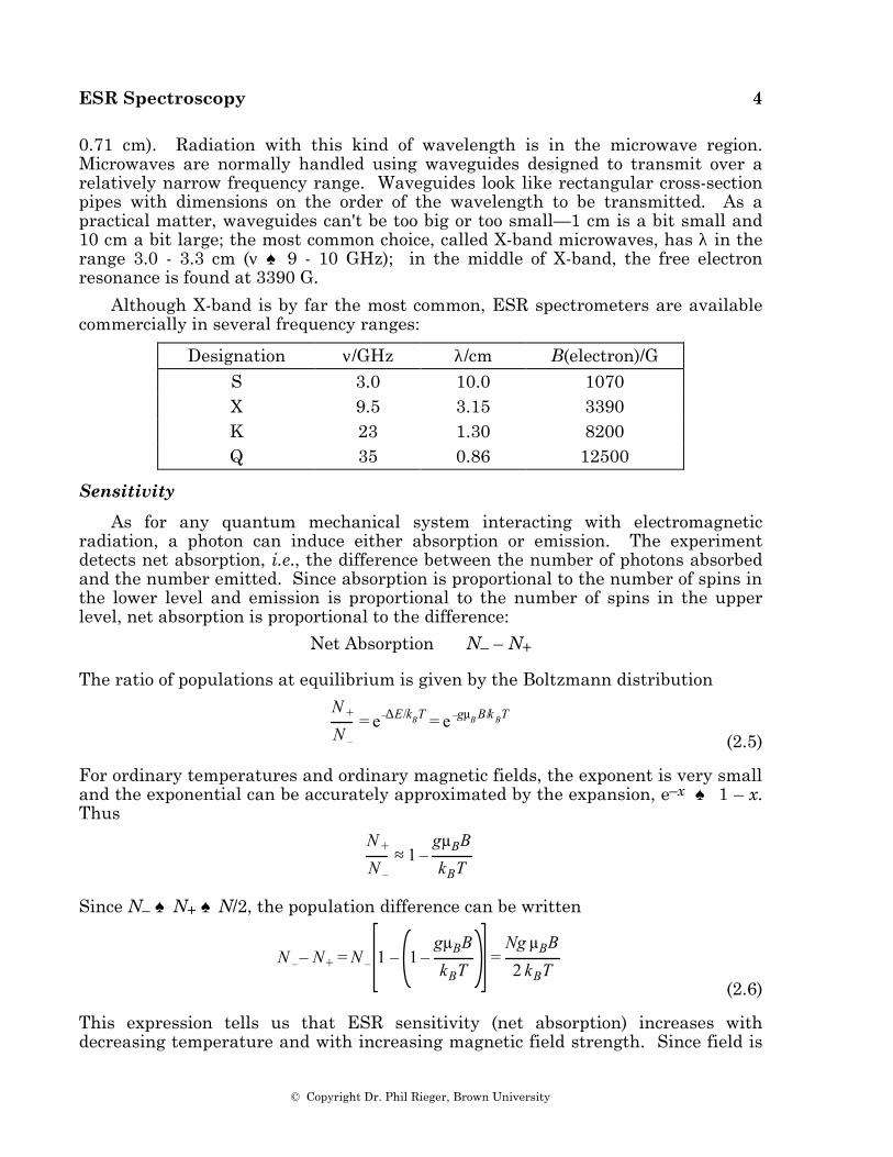
Although X-band is by far the most common, ESR spectrometers are available commercially in several frequency ranges:

Designation ν/GHz λ/cm B(electron)/G S 3.0 10.0 1070 X 9.5 3.15 3390 K 23 1.30 8200 Q 35 0.86 12500

Sensitivity

As for any quantum mechanical system interacting with electromagnetic radiation, a photon can induce either absorption or emission. The experiment detects net absorption, i.e., the difference between the number of photons absorbed and the number emitted. Since absorption is proportional to the number of spins in the lower level and emission is proportional to the number of spins in the upper level, net absorption is proportional to the difference:

Net Absorption ∝ N– – N+

The ratio of populations at equilibrium is given by the Boltzmann distribution

N +

N –

= e–∆E/kBT = e –gµB B/k BT

(2.5)

For ordinary temperatures and ordinary magnetic fields, the exponent is very small and the exponential can be accurately approximated by the expansion, e–x ♠ 1 – x. Thus

N +

N –

≈ 1 –gµBB

kBT

Since N– ♠ N+ ♠ N/2, the population difference can be written

N – – N+ = N – 1 – 1 –

gµBB

kBT=

Ng µBB

2 kBT (2.6)

This expression tells us that ESR sensitivity (net absorption) increases with decreasing temperature and with increasing magnetic field strength. Since field is

ESR Spectroscopy 5


proportional to microwave frequency, in principle sensitivity should be greater for K-band or Q-band spectrometers than for X-band. However, since the K- or Q-band waveguides are smaller, samples are also necessarily smaller, usually more than canceling the advantage of a more favorable Boltzmann factor.

Under ideal conditions, a commercial X-band spectrometer can detect the order of 1012 spins (10–12 moles) at room temperature. By ideal conditions, we mean a single line, on the order of 0.1 G wide; sensitivity goes down roughly as the reciprocal square of the linewidth. When the resonance is split into two or more hyperfine lines, sensitivity goes down still further. Nonetheless, ESR is a remarkably sensitive technique, especially compared with NMR.

Saturation

Because the two spin levels are so nearly equally populated, magnetic resonance suffers from a problem not encountered in higher energy forms of spectroscopy: An intense radiation field will tend to equalize the populations, leading to a decrease in net absorption; this effect is called "saturation". A spin system returns to thermal equilibrium via energy transfer to the surroundings, a rate process called spin-lattice relaxation, with a characteristic time, T1, the spin-lattice relaxation time (rate constant = 1/T1). Systems with a long T1 (i.e., spin systems weakly coupled to the surroundings) will be easily saturated; those with shorter T1 will be more difficult to saturate. Since spin-orbit coupling provides an important energy transfer mechanism, we usually find that odd-electron species with light atoms (e.g., organic radicals) have long T1's, those with heavier atoms (e.g., organotransition metal radicals) have shorter T1's. The effect of saturation is considered in more detail in Appendix I, where the phenomenological Bloch equations are introduced.

Nuclear Hyperfine Interaction

When one or more magnetic nuclei interact with the unpaired electron, we have another perturbation of the electron energy, i.e., another term in the spin Hamiltonian:

H s = gµBB S z + AI ⋅S

(2.7)

(Strictly speaking we should include the nuclear Zeeman interaction, γBIz. However, in most cases the energy contributions are negligible on the ESR energy scale, and, since observed transitions are between levels with the same values of mI, the nuclear Zeeman energies cancel in computing ESR transition energies.) Expanding the dot product and substituting the raising and lowering operators for Sx, Sy, Ix, and Iy (

S ± = S x ± i S y, I ± = I x ± i I y ), we have

H s = gµBB S z + AI zS z + 1

2I +S - + I -S + (2.8)

Suppose that the nuclear spin is 1/2; operating on the spin functions, m S ,m I we

get:

ESR Spectroscopy 6


H s1 21 2,1 21 2 = 1

2gµB B + 1

4A 1 21 2,1 21 2

H s1 21 2,–1 21 2 = 1

2gµB B – 1

4A 1 21 2, –1 21 2 + 1

2A –1 21 2,1 21 2

H s –1 21 2,1 21 2 = – 12

gµBB – 14

A –1 21 2,1 21 2 + 12

A 1 21 2,–1 21 2

H s –1 21 2, –1 21 2 = – 12

gµBB + 14

A –1 21 2, –1 21 2

The Hamiltonian matrix thus is

12 gµBB +

14 A 0 0 0

012 gµBB –

14 A

12 A 0

012 A –

12 gµBB –

14 A 0

0 0 0 –12 gµBB +

14 A

(2.9)

If the hyperfine coupling is sufficiently small, A << gµBB, the diagonal elements, which correspond to the energies to first-order in perturbation theory, will be sufficiently accurate:

E = ± 1

2gµBB ± 1

4A

(2.10)

However, for large A, the matrix must be diagonalized. This is easy when there is only one hyperfine coupling:

E 1 21 2,1 21 2 = 1

2 gµBB + 14 A

(2.11a)

E –1 21 2, –1 21 2 = – 1

2 gµBB + 14 A

(2.11b)

E 1 21 2, –1 21 2 = – 1

4 A + 12 gµBB 1 +

AgµBB

2

(2.11c)

E –1 21 2,1 21 2 = – 1

4 A – 12 gµBB 1 +

AgµB B

2

(2.11d)

ESR Spectroscopy 7


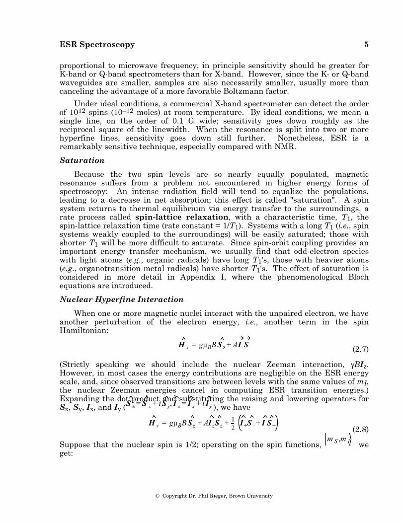
These equations are a special case of the general solution to eq (2.8), called the Breit-Rabi equation (10). The energies are plotted as functions of B in Figure 2.1 for g = 2.00, A = 0.1 cm–1. Notice that at zero field, there are two levels corresponding to a spin singlet (E = –3A/4) and a triplet (E = +A/4). At high field, the four levels divide into two higher levels (mS = +1/2) and two lower levels (mS = –1/2) and approach the first-order results, eq (2.10) (the first-order solution is called the high-field approx-imation). In order to conserve angular momentum, transitions among these levels can involve only one spin flip; in other words, the selection rules are ∆mS = ±1, ∆mI = 0 (ESR transitions) or ∆mS = 0, ∆mI = ±1 (NMR transitions); the latter involves much lower energy photons, and, in practice, only the ∆mS = ±1 transitions are observed. In Figure 2.1, these transitions are marked for a photon energy of 0.315 cm-1.

-0.3

-0.2

-0.1

0

0.1

0.2

0.3E/cm-1

0 1000 2000 3000 4000 5000B/Gauss

Figure 2.1. Energy levels for an electron interacting with a spin 1/2 nucleus, g = 2.00, A = 0.10 cm–1. The arrows show the transitions induced by 0.315 cm-1 radiation.

3. Operation of an ESR Spectrometer

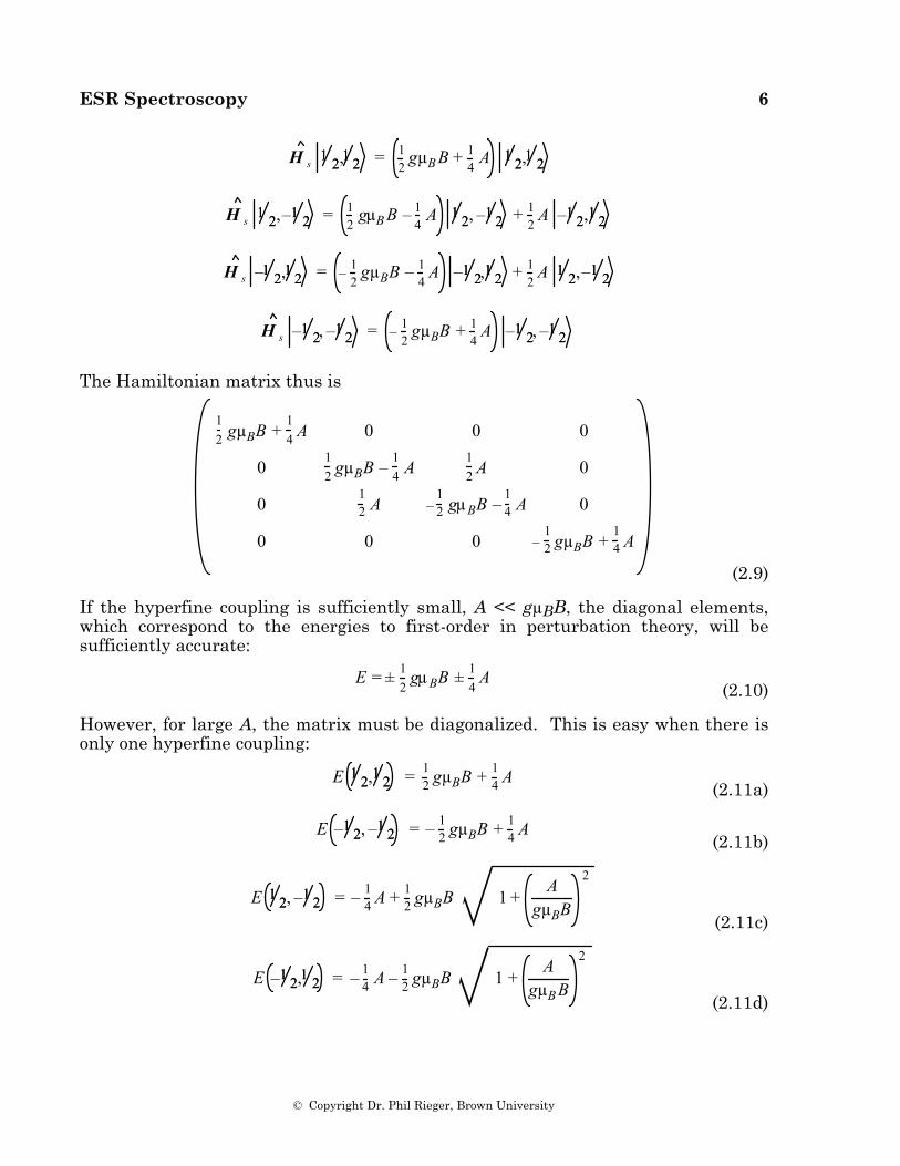
Although many spect-rometer designs have been produced over the years, the vast majority of lab-oratory instruments are based on the simplified block diagram shown in Figure 3.1. Microwaves are generated by the Klystron tube and the power level adjusted with the Attenuator. The Circulator behaves like a traffic circle: microwaves entering from the Klystron are routed toward the Cavity where the sample is

Klystron Attenuator

Load

Circulator

Magnet

Cavity

µ-Ammeter

Diode Detector

Figure 3.1. Block diagram of an ESR spectrometer.

mounted. Microwaves reflected back from the cavity (less when power is being absorbed) are routed to the diode detector, and any power reflected from the diode is

ESR Spectroscopy 8


absorbed completely by the Load. The diode is mounted along the E-vector of the plane-polarized microwaves and thus produces a current proportional to the microwave power reflected from the cavity. Thus, in principle, the absorption of microwaves by the sample could be detected by noting a decrease in current in the microammeter. In practice, of course, such a d.c. measurement would be far too noisy to be useful.

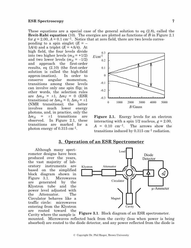
The solution to the signal-to-noise ratio problem is to introduce small amplitude field modulation. An oscillating magnetic field is super-imposed on the d.c. field by means of small coils, usually built into the cavity walls. When the field is in the vicinity of a resonance line, it is swept back and forth through part of the line, leading to an a.c. component in the diode current. This a.c. component is amplified using a frequency selective amplifier, thus eliminating a great deal of noise. The modulation amplitude is normally less than the line width. Thus the detected

Abs

orpt

ion

2nd

deri

vativ

e

Magnetic Field Strength

1st-

deri

vativ

e

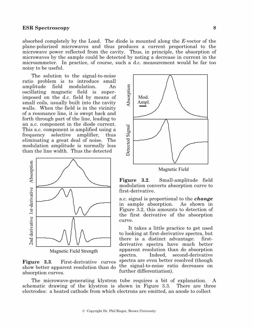
Figure 3.3. First-derivative curves show better apparent resolution than do absorption curves.

Det

ecte

d Si

gnal

Magnetic Field

Abs

orpt

ion

Mod.Ampl.

Figure 3.2. Small-amplitude field modulation converts absorption curve to first-derivative.

a.c. signal is proportional to the change in sample absorption. As shown in Figure 3.2, this amounts to detection of the first derivative of the absorption curve.

It takes a little practice to get used to looking at first-derivative spectra, but there is a distinct advantage: first-derivative spectra have much better apparent resolution than do absorption spectra. Indeed, second-derivative spectra are even better resolved (though the signal-to-noise ratio decreases on further differentiation).

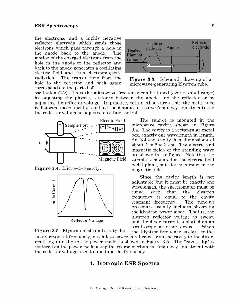
The microwave-generating klystron tube requires a bit of explanation. A schematic drawing of the klystron is shown in Figure 3.3. There are three electrodes: a heated cathode from which electrons are emitted, an anode to collect

ESR Spectroscopy 9


the electrons, and a highly negative reflector electrode which sends those electrons which pass through a hole in the anode back to the anode. The motion of the charged electrons from the hole in the anode to the reflector and back to the anode generates a oscillating electric field and thus electromagnetic radiation. The transit time from the hole to the reflector and back again corresponds to the period of

Electron pathway

Reflector electrodeAnodeHeated

filament cathode

Figure 3.3. Schematic drawing of a microwave-generating klystron tube.

oscillation (1/ν). Thus the microwave frequency can be tuned (over a small range) by adjusting the physical distance between the anode and the reflector or by adjusting the reflector voltage. In practice, both methods are used: the metal tube is distorted mechanically to adjust the distance (a coarse frequency adjustment) and the reflector voltage is adjusted as a fine control.

Electric Field

Magnetic Field

Sample Port

Iris

Figure 3.4. Microwave cavity.

Dio

de C

urre

nt

Reflector Voltage

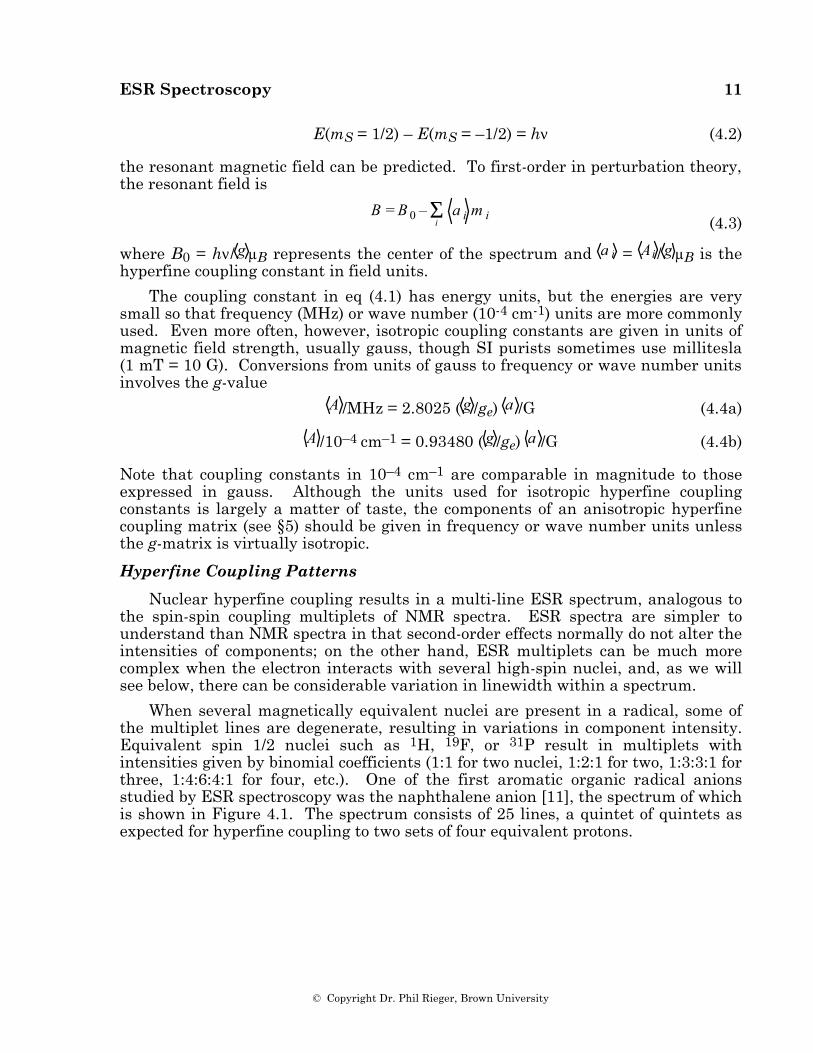
Figure 3.5. Klystron mode and cavity dip.

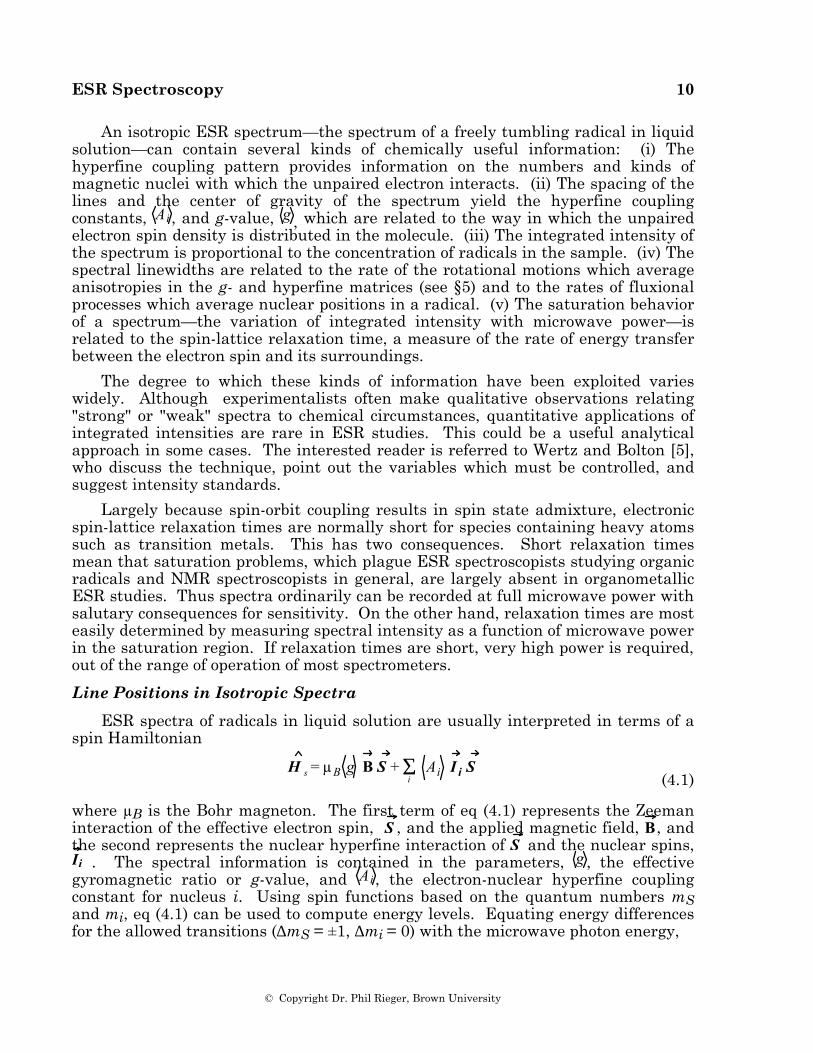
The sample is mounted in the microwave cavity, shown in Figure 3.4. The cavity is a rectangular metal box, exactly one wavelength in length. An X-band cavity has dimensions of about 1 ∞ 2 ∞ 3 cm. The electric and magnetic fields of the standing wave are shown in the figure. Note that the sample is mounted in the electric field nodal plane, but at a maximum in the magnetic field.

Since the cavity length is not adjustable but it must be exactly one wavelength, the spectrometer must be tuned such that the klystron frequency is equal to the cavity resonant frequency. The tune-up procedure usually includes observing the klystron power mode. That is, the klystron reflector voltage is swept, and the diode current is plotted on an oscilloscope or other device. When the klystron frequency is close to the

cavity resonant frequency, much less power is reflected from the cavity to the diode, resulting in a dip in the power mode as shown in Figure 3.5. The "cavity dip" is centered on the power mode using the coarse mechanical frequency adjustment with the reflector voltage used to fine tune the frequency.

4. Isotropic ESR Spectra

ESR Spectroscopy 10


An isotropic ESR spectrum—the spectrum of a freely tumbling radical in liquid solution—can contain several kinds of chemically useful information: (i) The hyperfine coupling pattern provides information on the numbers and kinds of magnetic nuclei with which the unpaired electron interacts. (ii) The spacing of the lines and the center of gravity of the spectrum yield the hyperfine coupling constants, Ai , and g-value, g , which are related to the way in which the unpaired electron spin density is distributed in the molecule. (iii) The integrated intensity of the spectrum is proportional to the concentration of radicals in the sample. (iv) The spectral linewidths are related to the rate of the rotational motions which average anisotropies in the g- and hyperfine matrices (see §5) and to the rates of fluxional processes which average nuclear positions in a radical. (v) The saturation behavior of a spectrum—the variation of integrated intensity with microwave power—is related to the spin-lattice relaxation time, a measure of the rate of energy transfer between the electron spin and its surroundings.

The degree to which these kinds of information have been exploited varies widely. Although experimentalists often make qualitative observations relating "strong" or "weak" spectra to chemical circumstances, quantitative applications of integrated intensities are rare in ESR studies. This could be a useful analytical approach in some cases. The interested reader is referred to Wertz and Bolton [5], who discuss the technique, point out the variables which must be controlled, and suggest intensity standards.

Largely because spin-orbit coupling results in spin state admixture, electronic spin-lattice relaxation times are normally short for species containing heavy atoms such as transition metals. This has two consequences. Short relaxation times mean that saturation problems, which plague ESR spectroscopists studying organic radicals and NMR spectroscopists in general, are largely absent in organometallic ESR studies. Thus spectra ordinarily can be recorded at full microwave power with salutary consequences for sensitivity. On the other hand, relaxation times are most easily determined by measuring spectral intensity as a function of microwave power in the saturation region. If relaxation times are short, very high power is required, out of the range of operation of most spectrometers.

Line Positions in Isotropic Spectra

ESR spectra of radicals in liquid solution are usually interpreted in terms of a spin Hamiltonian

H s = µB g B⋅S + Ai I i⋅SΣ

i (4.1)

where µB is the Bohr magneton. The first term of eq (4.1) represents the Zeeman interaction of the effective electron spin, S , and the applied magnetic field, B, and the second represents the nuclear hyperfine interaction of S and the nuclear spins, Ii . The spectral information is contained in the parameters, g , the effective gyromagnetic ratio or g-value, and Ai , the electron-nuclear hyperfine coupling constant for nucleus i. Using spin functions based on the quantum numbers mS and mi, eq (4.1) can be used to compute energy levels. Equating energy differences for the allowed transitions (∆mS = ±1, ∆mi = 0) with the microwave photon energy,

ESR Spectroscopy 11


E(mS = 1/2) – E(mS = –1/2) = hν (4.2)

the resonant magnetic field can be predicted. To first-order in perturbation theory, the resonant field is

B = B 0 – a i m iΣ

i (4.3)

where B0 = hν/ g µB represents the center of the spectrum and a i = Ai / g µB is the hyperfine coupling constant in field units.

The coupling constant in eq (4.1) has energy units, but the energies are very small so that frequency (MHz) or wave number (10-4 cm-1) units are more commonly used. Even more often, however, isotropic coupling constants are given in units of magnetic field strength, usually gauss, though SI purists sometimes use millitesla (1 mT = 10 G). Conversions from units of gauss to frequency or wave number units involves the g-value

A /MHz = 2.8025 ( g /ge) a /G (4.4a)

A /10–4 cm–1 = 0.93480 ( g /ge) a /G (4.4b)

Note that coupling constants in 10–4 cm–1 are comparable in magnitude to those expressed in gauss. Although the units used for isotropic hyperfine coupling constants is largely a matter of taste, the components of an anisotropic hyperfine coupling matrix (see §5) should be given in frequency or wave number units unless the g-matrix is virtually isotropic.

Hyperfine Coupling Patterns

Nuclear hyperfine coupling results in a multi-line ESR spectrum, analogous to the spin-spin coupling multiplets of NMR spectra. ESR spectra are simpler to understand than NMR spectra in that second-order effects normally do not alter the intensities of components; on the other hand, ESR multiplets can be much more complex when the electron interacts with several high-spin nuclei, and, as we will see below, there can be considerable variation in linewidth within a spectrum.

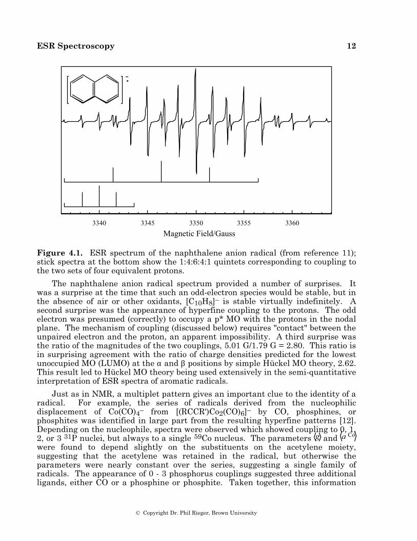
When several magnetically equivalent nuclei are present in a radical, some of the multiplet lines are degenerate, resulting in variations in component intensity. Equivalent spin 1/2 nuclei such as 1H, 19F, or 31P result in multiplets with intensities given by binomial coefficients (1:1 for two nuclei, 1:2:1 for two, 1:3:3:1 for three, 1:4:6:4:1 for four, etc.). One of the first aromatic organic radical anions studied by ESR spectroscopy was the naphthalene anion [11], the spectrum of which is shown in Figure 4.1. The spectrum consists of 25 lines, a quintet of quintets as expected for hyperfine coupling to two sets of four equivalent protons.

ESR Spectroscopy 12


3340 3345 3350 3355 3360

Magnetic Field/Gauss

Figure 4.1. ESR spectrum of the naphthalene anion radical (from reference 11); stick spectra at the bottom show the 1:4:6:4:1 quintets corresponding to coupling to the two sets of four equivalent protons.

The naphthalene anion radical spectrum provided a number of surprises. It was a surprise at the time that such an odd-electron species would be stable, but in the absence of air or other oxidants, [C10H8]– is stable virtually indefinitely. A second surprise was the appearance of hyperfine coupling to the protons. The odd electron was presumed (correctly) to occupy a p* MO with the protons in the nodal plane. The mechanism of coupling (discussed below) requires "contact" between the unpaired electron and the proton, an apparent impossibility. A third surprise was the ratio of the magnitudes of the two couplings, 5.01 G/1.79 G = 2.80. This ratio is in surprising agreement with the ratio of charge densities predicted for the lowest unoccupied MO (LUMO) at the α and β positions by simple Hückel MO theory, 2.62. This result led to Hückel MO theory being used extensively in the semi-quantitative interpretation of ESR spectra of aromatic radicals.

Just as in NMR, a multiplet pattern gives an important clue to the identity of a radical. For example, the series of radicals derived from the nucleophilic displacement of Co(CO)4– from [(RCCR')Co2(CO)6]– by CO, phosphines, or phosphites was identified in large part from the resulting hyperfine patterns [12]. Depending on the nucleophile, spectra were observed which showed coupling to 0, 1, 2, or 3 31P nuclei, but always to a single 59Co nucleus. The parameters g and a Co were found to depend slightly on the substituents on the acetylene moiety, suggesting that the acetylene was retained in the radical, but otherwise the parameters were nearly constant over the series, suggesting a single family of radicals. The appearance of 0 - 3 phosphorus couplings suggested three additional ligands, either CO or a phosphine or phosphite. Taken together, this information

ESR Spectroscopy 13


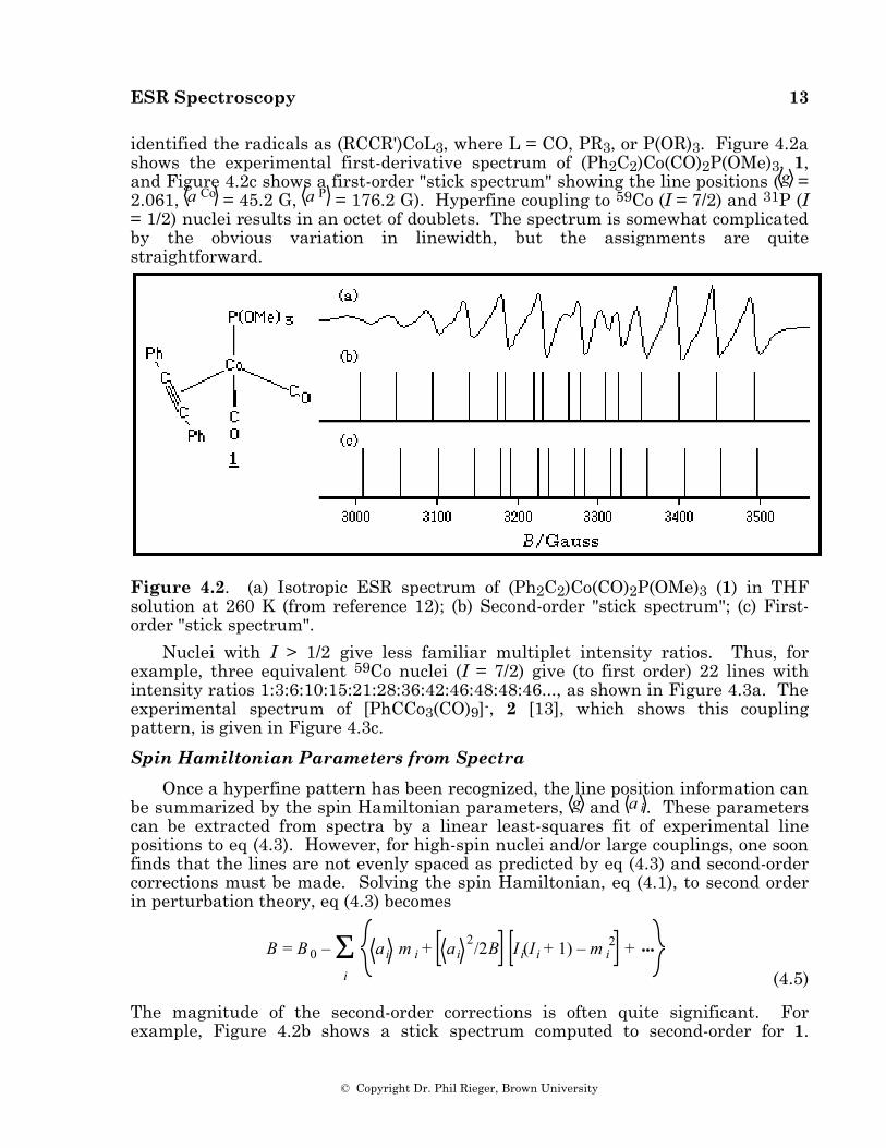
identified the radicals as (RCCR')CoL3, where L = CO, PR3, or P(OR)3. Figure 4.2a shows the experimental first-derivative spectrum of (Ph2C2)Co(CO)2P(OMe)3, 1, and Figure 4.2c shows a first-order "stick spectrum" showing the line positions ( g = 2.061, a Co = 45.2 G, a P = 176.2 G). Hyperfine coupling to 59Co (I = 7/2) and 31P (I = 1/2) nuclei results in an octet of doublets. The spectrum is somewhat complicated by the obvious variation in linewidth, but the assignments are quite straightforward.

Figure 4.2. (a) Isotropic ESR spectrum of (Ph2C2)Co(CO)2P(OMe)3 (1) in THF solution at 260 K (from reference 12); (b) Second-order "stick spectrum"; (c) First-order "stick spectrum".

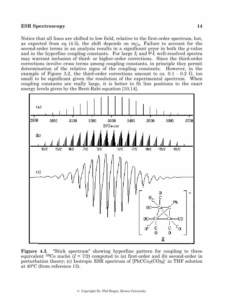
Nuclei with I > 1/2 give less familiar multiplet intensity ratios. Thus, for example, three equivalent 59Co nuclei (I = 7/2) give (to first order) 22 lines with intensity ratios 1:3:6:10:15:21:28:36:42:46:48:48:46..., as shown in Figure 4.3a. The experimental spectrum of [PhCCo3(CO)9]-, 2 [13], which shows this coupling pattern, is given in Figure 4.3c.

Spin Hamiltonian Parameters from Spectra

Once a hyperfine pattern has been recognized, the line position information can be summarized by the spin Hamiltonian parameters, g and a i . These parameters can be extracted from spectra by a linear least-squares fit of experimental line positions to eq (4.3). However, for high-spin nuclei and/or large couplings, one soon finds that the lines are not evenly spaced as predicted by eq (4.3) and second-order corrections must be made. Solving the spin Hamiltonian, eq (4.1), to second order in perturbation theory, eq (4.3) becomes

B = B 0 – a i m i + a i

2/2B I i(I i + 1) – m i2 +Σ

i (4.5)

The magnitude of the second-order corrections is often quite significant. For example, Figure 4.2b shows a stick spectrum computed to second-order for 1.

ESR Spectroscopy 14


Notice that all lines are shifted to low field, relative to the first-order spectrum, but, as expected from eq (4.5), the shift depends on mCo. Failure to account for the second-order terms in an analysis results in a significant error in both the g-value and in the hyperfine coupling constants. For large Ii and a i , well-resolved spectra may warrant inclusion of third- or higher-order corrections. Since the third-order corrections involve cross terms among coupling constants, in principle they permit determination of the relative signs of the coupling constants. However, in the example of Figure 3.2, the third-order corrections amount to ca. 0.1 - 0.2 G, too small to be significant given the resolution of the experimental spectrum. When coupling constants are really large, it is better to fit line positions to the exact energy levels given by the Breit-Rabi equation [10,14].

Figure 4.3. "Stick spectrum" showing hyperfine pattern for coupling to three equivalent 59Co nuclei (I = 7/2) computed to (a) first-order and (b) second-order in perturbation theory; (c) Isotropic ESR spectrum of [PhCCo3(CO)9]- in THF solution at 40°C (from reference 13).

ESR Spectroscopy 15


Second-order Splittings

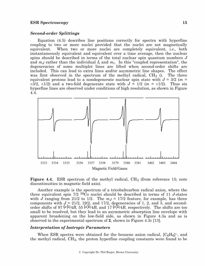
Equation (4.5) describes line positions correctly for spectra with hyperfine coupling to two or more nuclei provided that the nuclei are not magnetically equivalent. When two or more nuclei are completely equivalent, i.e., both instantaneously equivalent and equivalent over a time average, then the nuclear spins should be described in terms of the total nuclear spin quantum numbers J and mJ rather than the individual Ii and mi. In this "coupled representation", the degeneracies of some multiplet lines are lifted when second-order shifts are included. This can lead to extra lines and/or asymmetric line shapes. The effect was first observed in the spectrum of the methyl radical, CH3 (). The three equivalent protons lead to a nondegenerate nuclear spin state with J = 3/2 (m = ±3/2, ±1/2) and a two-fold degenerate state with J = 1/2 (m = ±1/2). Thus six hyperfine lines are observed under conditions of high resolution, as shown in Figure 4.4.

3356 3357 3358

Magnetic Field/Gauss3333 3334 3335 3379 3380 3381 3402 3403 3404

Figure 4.4. ESR spectrum of the methyl radical, CH3 (from reference 15; note discontinuities in magnetic field axis).

Another example is the spectrum of a tricobaltcarbon radical anion, where the three equivalent spin 7/2 59Co nuclei should be described in terms of 11 J-states with J ranging from 21/2 to 1/2. The mJ = 17/2 feature, for example, has three components with J = 21/2, 19/2, and 17/2, degeneracies of 1, 2, and 3, and second-order shifts of 97 a 2/4B, 55 a 2/4B, and 17 a 2/4B, respectively. The shifts are too small to be resolved, but they lead to an asymmetric absorption line envelope with apparent broadening on the low-field side, as shown in Figure 4.3a and as is observed in the experimental spectrum of 2, shown in Figure 4.3c [13].

Interpretation of Isotropic Parameters

When ESR spectra were obtained for the benzene anion radical, [C6H6]–, and the methyl radical, CH3, the proton hyperfine coupling constants were found to be

ESR Spectroscopy 16


3.75 G and 23.0 G, respectively. Since each carbon atom of the benzene anion carries an electron spin density of 1/6, the two results suggest that the proton coupling to an electron in a p* orbital is proportional to the spin density on the adjacent carbon atom,

a H = QCHH ρCp (4.6)

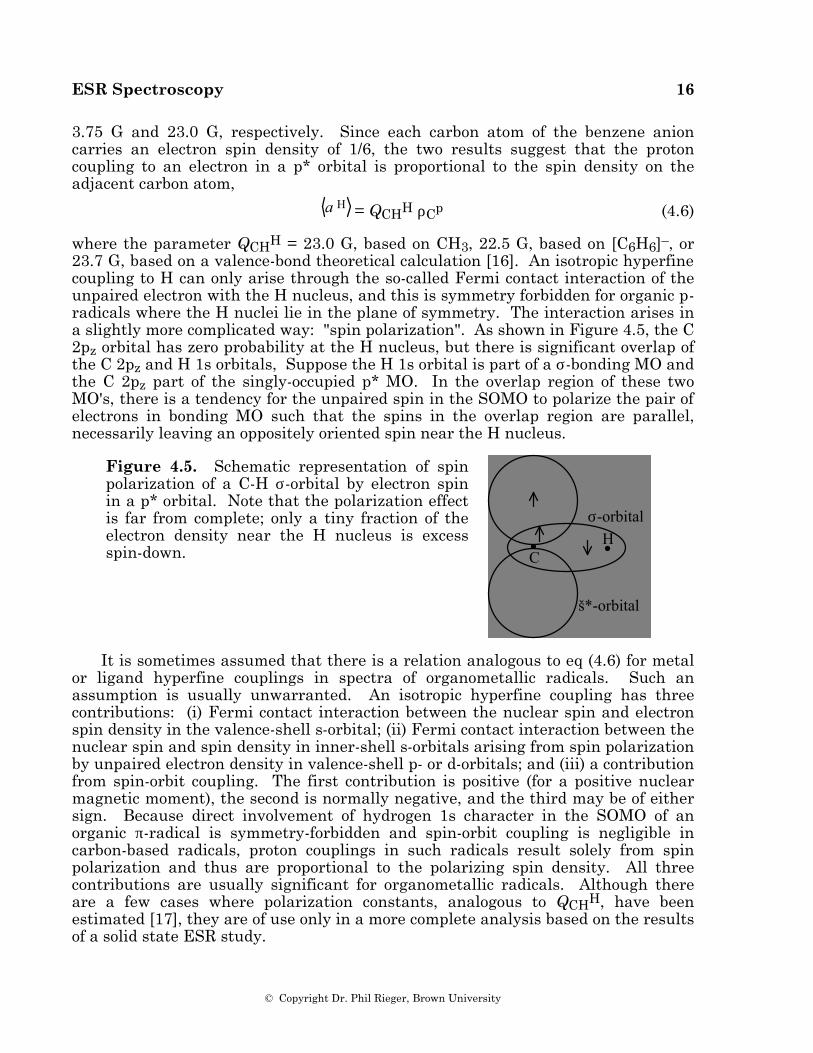
where the parameter QCHH = 23.0 G, based on CH3, 22.5 G, based on [C6H6]–, or 23.7 G, based on a valence-bond theoretical calculation [16]. An isotropic hyperfine coupling to H can only arise through the so-called Fermi contact interaction of the unpaired electron with the H nucleus, and this is symmetry forbidden for organic p-radicals where the H nuclei lie in the plane of symmetry. The interaction arises in a slightly more complicated way: "spin polarization". As shown in Figure 4.5, the C 2pz orbital has zero probability at the H nucleus, but there is significant overlap of the C 2pz and H 1s orbitals, Suppose the H 1s orbital is part of a σ-bonding MO and the C 2pz part of the singly-occupied p* MO. In the overlap region of these two MO's, there is a tendency for the unpaired spin in the SOMO to polarize the pair of electrons in bonding MO such that the spins in the overlap region are parallel, necessarily leaving an oppositely oriented spin near the H nucleus.

Figure 4.5. Schematic representation of spin polarization of a C-H σ-orbital by electron spin in a p* orbital. Note that the polarization effect is far from complete; only a tiny fraction of the electron density near the H nucleus is excess spin-down.

HC

š*-orbital

σ-orbital

It is sometimes assumed that there is a relation analogous to eq (4.6) for metal or ligand hyperfine couplings in spectra of organometallic radicals. Such an assumption is usually unwarranted. An isotropic hyperfine coupling has three contributions: (i) Fermi contact interaction between the nuclear spin and electron spin density in the valence-shell s-orbital; (ii) Fermi contact interaction between the nuclear spin and spin density in inner-shell s-orbitals arising from spin polarization by unpaired electron density in valence-shell p- or d-orbitals; and (iii) a contribution from spin-orbit coupling. The first contribution is positive (for a positive nuclear magnetic moment), the second is normally negative, and the third may be of either sign. Because direct involvement of hydrogen 1s character in the SOMO of an organic π-radical is symmetry-forbidden and spin-orbit coupling is negligible in carbon-based radicals, proton couplings in such radicals result solely from spin polarization and thus are proportional to the polarizing spin density. All three contributions are usually significant for organometallic radicals. Although there are a few cases where polarization constants, analogous to QCHH, have been estimated [17], they are of use only in a more complete analysis based on the results of a solid state ESR study.

ESR Spectroscopy 17


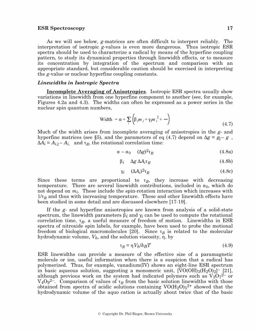
As we will see below, g-matrices are often difficult to interpret reliably. The interpretation of isotropic g-values is even more dangerous. Thus isotropic ESR spectra should be used to characterize a radical by means of the hyperfine coupling pattern, to study its dynamical properties through linewidth effects, or to measure its concentration by integration of the spectrum and comparison with an appropriate standard, but considerable caution should be exercised in interpreting the g-value or nuclear hyperfine coupling constants.

Linewidths in Isotropic Spectra

Incomplete Averaging of Anisotropies. Isotropic ESR spectra usually show variations in linewidth from one hyperfine component to another (see, for example, Figures 4.2a and 4.3). The widths can often be expressed as a power series in the nuclear spin quantum numbers,

Width = α+ β im i + γim i

2 +Σi (4.7)

Much of the width arises from incomplete averaging of anisotropies in the g- and hyperfine matrices (see §5), and the parameters of eq (4.7) depend on ∆g = g|| – g⊥, ∆Ai = Ai,|| – Ai,⊥ and τR, the rotational correlation time:

α – α0 ∝ (∆g)2τR (4.8a)

βi ∝ ∆g ∆AiτR (4.8b)

γi ∝ (∆Ai)2τR (4.8c)

Since these terms are proportional to τR, they increase with decreasing temperature. There are several linewidth contributions, included in α0, which do not depend on mi. These include the spin-rotation interaction which increases with 1/τR and thus with increasing temperature. These and other linewidth effects have been studied in some detail and are discussed elsewhere [17-19].

If the g- and hyperfine anisotropies are known from analysis of a solid-state spectrum, the linewidth parameters βi and γi can be used to compute the rotational correlation time, τR, a useful measure of freedom of motion. Linewidths in ESR spectra of nitroxide spin labels, for example, have been used to probe the motional freedom of biological macromolecules [20]. Since τR is related to the molecular hydrodynamic volume, Vh, and the solution viscosity, η, by

τR = ηVh/kBT (4.9)

ESR linewidths can provide a measure of the effective size of a paramagnetic molecule or ion, useful information when there is a suspicion that a radical has polymerized. Thus, for example, vanadium(IV) shows an eight-line ESR spectrum in basic aqueous solution, suggesting a monomeric unit, [VO(OH)3(H2O)2]– [21], although previous work on the system had indicated polymers such as V3O72– or V4O92–. Comparison of values of τR from the basic solution linewidths with those obtained from spectra of acidic solutions containing VO(H2O)52+ showed that the hydrodynamic volume of the aquo cation is actually about twice that of the basic

ESR Spectroscopy 18


solution species, effectively ruling out the presence of ESR-active polymers in solution [22].

Rates of Fluxionality from Linewidths. ESR linewidths are also sensitive to processes which modulate the g-value or hyperfine coupling constants or limit the lifetime of the electron spin state. The effects are closely analogous to those observed in NMR spectra of dynamical systems. However, since ESR linewidths are typically on the order of 0.1-10 G (0.3-30 MHz), rate processes which give observable increases in linewidths must be fast. Bimolecular processes which contribute to ESR linewidths have mostly been nearly diffusion-controlled, e.g., intermolecular electron exchange between naphthalene and its anion radical [23] and reversible axial ligation of square planar copper(II) complexes [24].

The effect of rate processes on linewidths can be understood quantitatively in terms of the modified Bloch equations ([25], see also Appendix 3), or, more accurately, in terms of density matrix [26] or relaxation matrix [18,27] formalisms. If a rate process modulates a line position through an amplitude ∆B (∆ω in angular frequency units) by fluctuating between two states, each with lifetime τ, a single line is observed with an excess width proportional to (∆ω)2τ when τ–1 >> ∆ω—the fast exchange limit. As the lifetime increases, the line broadens to indetectability and then re-emerges as two broad lines. These shift apart and sharpen until, in the slow exchange limit (τ-1 << ∆ω), two lines are observed with widths proportional to τ-1.

ESR Spectroscopy 19


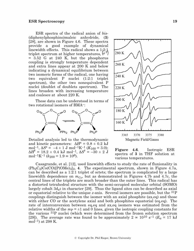
ESR spectra of the radical anion of bis-(diphenylphosphino)maleic anhydride, (3) [28], are shown in Figure 4.6. These spectra provide a good example of dynamical linewidth effects. This radical shows a 1:2:1 triplet spectrum at higher temperatures, a P = 3.52 G at 240 K, but the phosphorus coupling is strongly temperature dependent and extra lines appear at 200 K and below indicating a dynamical equilibrium between two isomeric forms of the radical, one having two equivalent P nuclei (1:2:1 triplet spectrum), the other two nonequivalent P nuclei (doublet of doublets spectrum). The lines broaden with increasing temperature and coalesce at about 220 K.

These data can be understood in terms of two rotational isomers of BMA–:

CC

Ph2P PPh2

C CO OO

CC

Ph2P Ph2P

C CO OO

Detailed analysis led to the thermodynamic and kinetic parameters: ∆H° = 0.8 ± 0.2 kJ mol–1, ∆S° = –4 ± 1 J mol–1K–1 (K160 = 3.0); ∆H† = 18.2 ± 0.4 kJ mol–1, ∆S† = –30 ± 2 J mol–1K–1 (k200 = 1.9 ∞ 106).

3365 3370 3375 3380Magnetic Field/Gauss

280 K

260 K

240 K

220 K

200 K

180 K

160 K

Figure 4.6. Isotropic ESR spectra of 3 in THF solution at various temperatures.

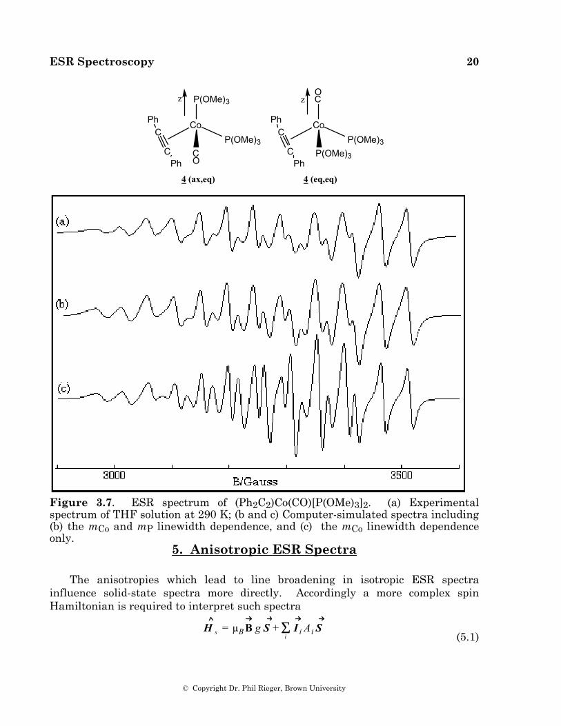
Casagrande, et al. [12], used linewidth effects to study the rate of fluxionality in (Ph2C2)Co(CO)[P(OMe)3]2, 4. The experimental spectrum, shown in Figure 4.7a, can be described as a 1:2:1 triplet of octets; the spectrum is complicated by a large linewidth dependence on mCo, but as demonstrated in Figures 4.7b and 4.7c, the central lines of the triplets are much broader than the outer lines. This radical has a distorted tetrahedral structure with the semi-occupied molecular orbital (SOMO) largely cobalt 3dz2 in character [29]. Thus the ligand sites can be described as axial or equatorial relative to the unique z-axis. Several isomers are possible, but the 31P couplings distinguish between the isomer with an axial phosphite (ax,eq) and those with either CO or the acetylene axial and both phosphites equatorial (eq,eq). The rate of interconversion between eq,eq and ax,eq isomers was estimated from the relative widths of the mP = ±1 and 0 lines, given the isotropic coupling constants for the various 31P nuclei (which were determined from the frozen solution spectrum [29]). The average rate was found to be approximately 2 ∞ 1010 s–1 (Ea = 17 kJ mol–1) at 298 K.

ESR Spectroscopy 20


Co

P(OMe)3

P(OMe)3

C O

CoC

CPh

Ph

O C

P(OMe)3

P(OMe)3

C

CPh

Ph

z z

4 (ax,eq) 4 (eq,eq)

Figure 3.7. ESR spectrum of (Ph2C2)Co(CO)[P(OMe)3]2. (a) Experimental spectrum of THF solution at 290 K; (b and c) Computer-simulated spectra including (b) the mCo and mP linewidth dependence, and (c) the mCo linewidth dependence only.

5. Anisotropic ESR Spectra

The anisotropies which lead to line broadening in isotropic ESR spectra influence solid-state spectra more directly. Accordingly a more complex spin Hamiltonian is required to interpret such spectra

H s = µB B⋅g⋅S + I i⋅Ai⋅SΣ

i (5.1)

ESR Spectroscopy 21


In eq (5.1), g and Ai are 3∞3 matrices representing the anisotropic Zeeman and nuclear hyperfine interactions. In general, a coordinate system can be found—the g-matrix principal axes—in which g is diagonal. If g and Ai are diagonal in the same coordinate system, we say that their principal axes are coincident.

In species with two or more unpaired electrons, a fine structure term must be added to the spin Hamiltonian to represent electron spin-spin interactions. We will confine our attention here to radicals with one unpaired electron (S = 1/2) but will address the S > 1/2 problem in Section 6.

Nuclear quadrupole interactions introduce line shifts and forbidden transitions in spectra of radicals with nuclei having I > 1/2. In practice, quadrupolar effects are observable only in very well-resolved spectra or in spectra of radicals with nuclei having small magnetic moments and large quadrupole moments. The most extreme case of a small magnetic moment to quadrupole moment ratio is that of 191Ir/193Ir, and spectra of [Ir(CN)6]3– [30], [Ir(CN)5Cl]4– and [Ir(CN)4Cl2]4– [31], and [Ir2(CO)2(PPh3)2(µ-RNNNR)2]+, R = p-tolyl [32], show easily recognizable quadrupolar effects. Other nuclei for which quadrupolar effects might be expected include 151Eu/153Eu, 155Gd/157Gd, 175Lu, 181Ta, 189Os, and 197Au. When quadrupolar effects are important, it is usually necessary to take account of the nuclear Zeeman interaction as well. The nuclear quadrupole and nuclear Zeeman interactions add two more terms to the spin Hamiltonian. Since these terms considerably complicate an already complex situation, we will confine our attention here to nuclei for which quadrupolar effects can be neglected.

When a radical is oriented such that the magnetic field direction is located by the polar and azimuthal angles, θ and φ, relative to the g-matrix principal axes, the resonant field is given, to first order in perturbation theory, by [33]

B = B 0 –

Aim i

gµB•

i (5.2)

where B 0 = h ν

gµB (5.3)

g2 = gx2 sin2θ cos2φ + gy2 sin2θ sin2φ + gz2cos2θ (5.4)

Ai2 = Aiz2 Six2 + Aiy2 Siy2 + Aiz2 Siz2 (5.5)

Sik = [gx sin θ cos φ lixk + gy sin θ cos φ liyk + gz cos θ lizk]/g (5.6)

and the lijk are direction cosines indicating the orientation of the kth principal axis of the ith hyperfine matrix relative to the jth g-matrix principal axis. When the matrix principal axes are coincident, only one of the lijk of eq (4.6) will be nonzero. When the hyperfine matrix components are large, second-order terms [33] must be added to eq (5.2); these result in down-field shifts, proportional to mi2.

Solid-State ESR Spectra

So long as they are dilute (to avoid line broadening from intermolecular spin exchange), radicals can be studied in the solid state as solutes in single crystals,

ESR Spectroscopy 22


powders, glasses or frozen solutions. Radicals can be produced in situ by UV- or γ-irradiation of a suitable precursor in a crystalline or glassy matrix. While many organometallic radicals have been studied in this way [34], it is often easier to obtain solid state ESR spectra by freezing the liquid solution in which the radical is formed. A variety of techniques then can be used to generate radicals, e.g., chemical reactions, electrochemical reduction or oxidation, or photochemical methods. Furthermore, the radical is studied under conditions more closely approximating those in which its reaction chemistry is known.

Spectra of Dilute Single Crystals. Spectra of radicals in a dilute single crystal are obtained for a variety of orientations, usually with the field perpendicular to one of the crystal axes. Spectra usually can be analyzed as if they were isotropic to obtain an effective g-value and hyperfine coupling constants. Since the g- and hyperfine matrix principal axes are not necessarily the same as the crystal axes, the matrices, written in the crystal axis system usually will have off-diagonal elements. Thus, for example, if spectra are obtained for a variety of orientations in the crystal xy-plane, the effective g-value is

gφ2 = (gxx cos φ + gyx sin φ)2 + (gxy cos φ + gyy sin φ)2 + (gxz cos φ + gyz sin φ)2 (5.7)

or gφ2 = K1+ K2 cos 2φ + K3 sin 2φ (5.8)

where K1 = (gxx2 + gyy2 + gxz2 + gyz2 + 2 gxy2)/2 (5.9a)

K2 = (gxx2 - gyy2 + gxz2 - gyz2)/2 (5.9b)

K3 = gxy(gxx + gyy) + gxzgyz (5.9c)

A sinusoidal plot of gφ2 vs φ can be analyzed to determine K1, K2, and K3. Exploration of another crystal plane gives another set of K's which depend on other combinations of the gij; eventually enough data are obtained to determine the six independent gij (g is a symmetric matrix so that gij = gji). The g2-matrix then is diagonalized to obtain the principal values and the transformation matrix, elements of which are the direction cosines of the g-matrix principal axes relative to the crystal axes. An analogous treatment of the effective hyperfine coupling constants leads to the principal values of the A2-matrix and the orientation of its principal axes in the crystal coordinate system.

Analysis of Powder Spectra. Since ESR spectra are normally recorded as the first derivative of absorption vs. field, observable features in the spectrum of a powder correspond to molecular orientations for which the derivative is large in magnitude or changes in sign. For any spin Hamiltonian, there will be minimum and maximum resonant fields at which the absorption changes rapidly from zero, leading to a large value of the derivative and features which resemble positive-going and negative-going absorption lines. Peaks in the absorption envelope correspond to derivative sign changes and lead to features resembling isotropic derivative lines. The interpretation of a powder spectrum thus depends on the connection of the positions of these features to the g- and hyperfine matrix components.

ESR Spectroscopy 23


Early treatments of powder patterns attempted to deal with the spatial distribution of resonant fields by analytical mathematics [35]. This approach led to some valuable insights but the algebra is much too complex when nonaxial hyperfine matrices are involved. Consider the simplest case: a single resonance line without hyperfine structure. The resonant field is given by eq (5.3). Features in the first derivative spectrum correspond to discontinuities or turning points in the absorption spectrum which arise when B/ θ or B/ φ are zero,

ŽBŽθ

=hνµB

gz2 – g⊥

2

g3 sin θ cos θ = 0

(5.10a)

or

ŽBŽφ

=hνµB

gx2 – gy

2

g3 sin 2θ sin φ cos φ = 0 (5.10b)

These equations have three solutions: (i) θ = 0; (ii) θ= 90°, φ = 0; and (iii) θ = φ = 90°. Since θ and φ are in the g-matrix axis system, observable features are expected for those fields corresponding to orientations along the principal axes of the g-matrix. This being the case, the principal values of the g-matrix are obtained from a straightforward application of eq (5.3).

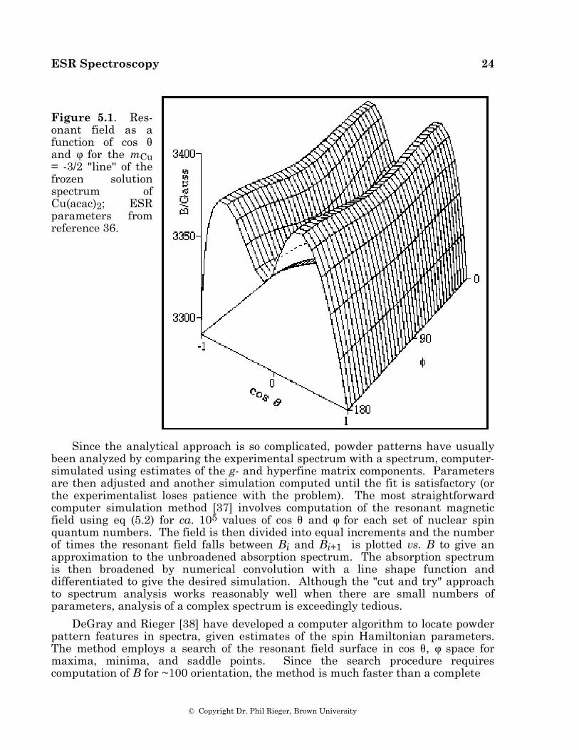
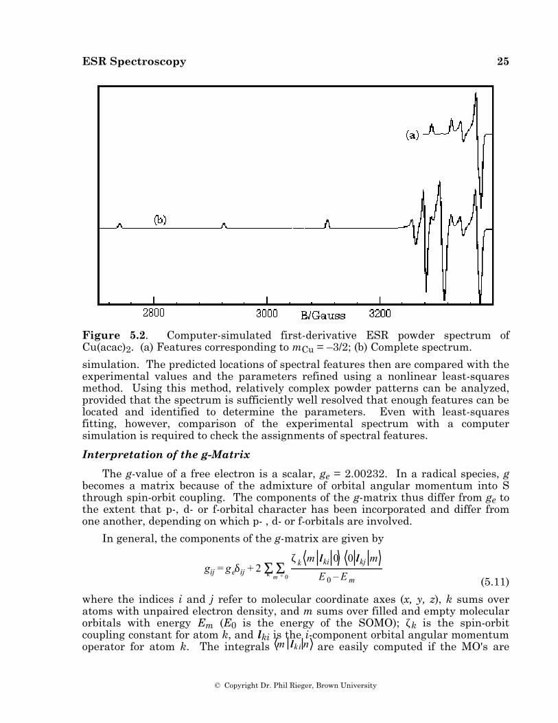
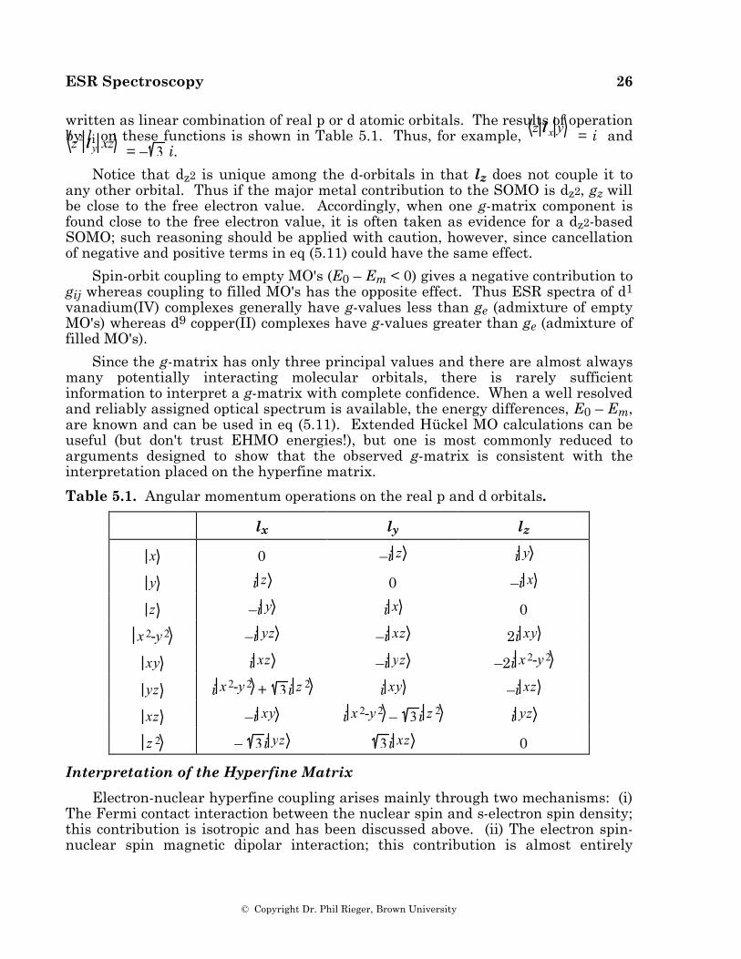
Powder spectra with hyperfine structure often can be interpreted similarly with spectral features identified with orientation of the magnetic field along one of the g- and hyperfine matrix principal axes. However, this simple situation often breaks down. Using a first-order theory and one hyperfine coupling, Ovchinnikov and Konstantinov [36] have shown that eqs (5.10) may have up to six solutions corresponding to observable spectral features. Three of these correspond to orientation of B along principal axes, but the "extra lines" correspond to less obvious orientations. Even more extra lines may creep in when the spin Hamiltonian is treated to second order or when there is more than one hyperfine coupling. The problem is illustrated by the resonant field vs. cos θ and φ surface shown in Figure 5.1, corresponding to the mCu = –3/2 "line" in the spectrum of Cu(acac)2 (g = 2.0527, 2.0570, 2.2514; ACu = 27.0, 19.5, 193.4 ∞ 10–4 cm–1) [36]. The minimum resonant field, B = 3290.7 G, corresponds to B along the z-axis (cos θ = ±1). With B along the x-axis (cos θ = 0, φ = 0°), the surface shows a saddle point at 3344.3 G, and with B along the y-axis (cos θ = 0, φ = 90°), there is a local minimum at 3325.5 G. In addition, another saddle point occurs in the yz-plane at B = 3371.2 G (cos θ = ±0.482, φ = 90°); the only maximum is in the xz-plane at B = 3379.0 G (cos θ = ± 0.459, , φ = 0°). Thus five features are expected and indeed are shown in the computer-simulated spectrum of Cu(acac)2 shown in Figure 5.2. The two high-field features correspond to off-axis field orientations and thus are "extra lines". The situation is more complex when the g- and hyperfine matrix principal axes are noncoincident (see below); in this case, none of the features need correspond to orientation of B along a principal axis direction.

ESR Spectroscopy 24


Figure 5.1. Res-onant field as a function of cos θ and φ for the mCu = -3/2 "line" of the frozen solution spectrum of Cu(acac)2; ESR parameters from reference 36.

Since the analytical approach is so complicated, powder patterns have usually been analyzed by comparing the experimental spectrum with a spectrum, computer-simulated using estimates of the g- and hyperfine matrix components. Parameters are then adjusted and another simulation computed until the fit is satisfactory (or the experimentalist loses patience with the problem). The most straightforward computer simulation method [37] involves computation of the resonant magnetic field using eq (5.2) for ca. 105 values of cos θ and φ for each set of nuclear spin quantum numbers. The field is then divided into equal increments and the number of times the resonant field falls between Bi and Bi+1 is plotted vs. B to give an approximation to the unbroadened absorption spectrum. The absorption spectrum is then broadened by numerical convolution with a line shape function and differentiated to give the desired simulation. Although the "cut and try" approach to spectrum analysis works reasonably well when there are small numbers of parameters, analysis of a complex spectrum is exceedingly tedious.

DeGray and Rieger [38] have developed a computer algorithm to locate powder pattern features in spectra, given estimates of the spin Hamiltonian parameters. The method employs a search of the resonant field surface in cos θ, φ space for maxima, minima, and saddle points. Since the search procedure requires computation of B for ~100 orientation, the method is much faster than a complete

ESR Spectroscopy 25


Figure 5.2. Computer-simulated first-derivative ESR powder spectrum of Cu(acac)2. (a) Features corresponding to mCu = –3/2; (b) Complete spectrum.

simulation. The predicted locations of spectral features then are compared with the experimental values and the parameters refined using a nonlinear least-squares method. Using this method, relatively complex powder patterns can be analyzed, provided that the spectrum is sufficiently well resolved that enough features can be located and identified to determine the parameters. Even with least-squares fitting, however, comparison of the experimental spectrum with a computer simulation is required to check the assignments of spectral features.

Interpretation of the g-Matrix

The g-value of a free electron is a scalar, ge = 2.00232. In a radical species, g becomes a matrix because of the admixture of orbital angular momentum into S through spin-orbit coupling. The components of the g-matrix thus differ from ge to the extent that p-, d- or f-orbital character has been incorporated and differ from one another, depending on which p- , d- or f-orbitals are involved.

In general, the components of the g-matrix are given by

gij = geδij + 2 Σκ

ζk m lki 0 0 lkj m

E 0 – E mΣ

m ° 0 (5.11)

where the indices i and j refer to molecular coordinate axes (x, y, z), k sums over atoms with unpaired electron density, and m sums over filled and empty molecular orbitals with energy Em (E0 is the energy of the SOMO); ζk is the spin-orbit coupling constant for atom k, and lki is the i-component orbital angular momentum operator for atom k. The integrals m lk i n are easily computed if the MO's are

ESR Spectroscopy 26


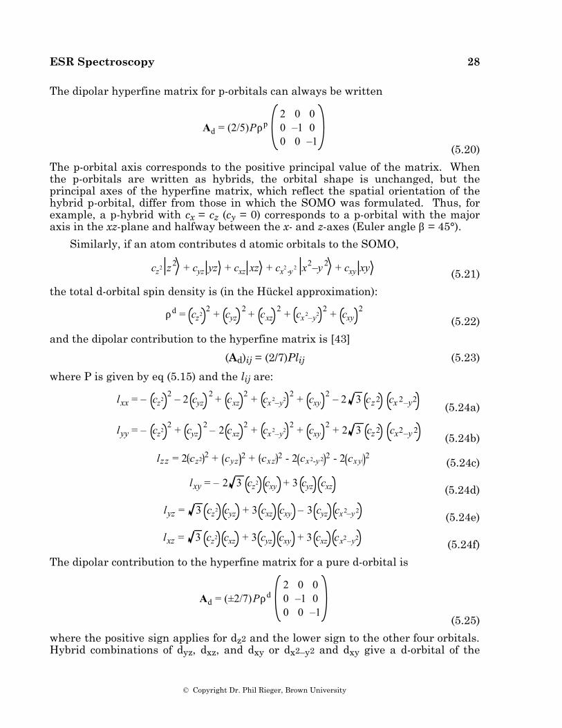
written as linear combination of real p or d atomic orbitals. The results of operation by li on these functions is shown in Table 5.1. Thus, for example,

z l x y = i and z 2 l y xz = – 3 i.

Notice that dz2 is unique among the d-orbitals in that lz does not couple it to any other orbital. Thus if the major metal contribution to the SOMO is dz2, gz will be close to the free electron value. Accordingly, when one g-matrix component is found close to the free electron value, it is often taken as evidence for a dz2-based SOMO; such reasoning should be applied with caution, however, since cancellation of negative and positive terms in eq (5.11) could have the same effect.

Spin-orbit coupling to empty MO's (E0 – Em < 0) gives a negative contribution to gij whereas coupling to filled MO's has the opposite effect. Thus ESR spectra of d1 vanadium(IV) complexes generally have g-values less than ge (admixture of empty MO's) whereas d9 copper(II) complexes have g-values greater than ge (admixture of filled MO's).

Since the g-matrix has only three principal values and there are almost always many potentially interacting molecular orbitals, there is rarely sufficient information to interpret a g-matrix with complete confidence. When a well resolved and reliably assigned optical spectrum is available, the energy differences, E0 – Em, are known and can be used in eq (5.11). Extended Hückel MO calculations can be useful (but don't trust EHMO energies!), but one is most commonly reduced to arguments designed to show that the observed g-matrix is consistent with the interpretation placed on the hyperfine matrix.

Table 5.1. Angular momentum operations on the real p and d orbitals.

lx ly lz

x 0 –i z i y

y i z 0 –i x

z –i y i x 0

x 2-y 2 –i yz –i xz 2i xy

xy i xz –i yz –2i x 2-y 2

yz i x 2-y 2 + 3i z 2 i xy –i xz

xz –i xy i x 2-y 2 – 3i z 2 i yz

z 2 – 3i yz 3i xz 0

Interpretation of the Hyperfine Matrix

Electron-nuclear hyperfine coupling arises mainly through two mechanisms: (i) The Fermi contact interaction between the nuclear spin and s-electron spin density; this contribution is isotropic and has been discussed above. (ii) The electron spin-nuclear spin magnetic dipolar interaction; this contribution is almost entirely

ESR Spectroscopy 27


anisotropic, i.e., neglecting spin-orbit coupling, the average dipolar contribution to the hyperfine coupling is zero.

The general form of the dipolar contribution to the hyperfine term of the Hamiltonian is

H dipolar = gegNµBµN ψSOMO

S ⋅I

r3–

3(S⋅r)(I⋅r)

r 5ψSOMO

(5.12)

where ge and gN are the electron and nuclear g-values, µB and µN are the Bohr and nuclear magnetons, and the matrix element is evaluated by integration over the spatial coordinates, leaving the spins as operators. Equation (5.12) can then be written

H dipolar = I ⋅Ad⋅S (5.13)

where Ad is the dipolar contribution to the hyperfine matrix,

A = •A E + Ad (5.14)

(E is the unit matrix). In evaluating the matrix element of eq (5.12), the integration over the angular variables is quite straightforward. The integral over r, however, requires a good atomic orbital wavefunction. Ordinarily, the integral is combined with the constants as a parameter

P = gegNµBµN r–3

(5.15)

P has been computed using Hartree-Fock atomic orbital wavefunctions and can be found in several published tabulations [39-42]. Because of the r -3 dependence of P, dipolar coupling of a nuclear spin with electron spin density on another atom is usually negligible.

If an atom contributes px, py, and pz atomic orbitals to the SOMO

cx x + cy y + cz z (5.16)

the total p-orbital spin density is (in the Hückel approximation, i.e., neglecting overlap):

ρp = cx2 + cy

2 + cz2 (5.17)

and the dipolar contribution to the hyperfine matrix can be written

(Ad)ij = (2/5)Plij (5.18)

where the lij are lxx = 2cx2 – cy

2 – cz2 (5.19a)

lyy = –cx2 + 2cy

2 – cz2 (5.19b)

lzz = –cx2 – cy

2 + 2cz2 (5.19c)

lij = –3cicj (i ? j) (5.19d)

ESR Spectroscopy 28


The dipolar hyperfine matrix for p-orbitals can always be written

Ad = (2/5)Pρp2 0 00 –1 00 0 –1

(5.20)

The p-orbital axis corresponds to the positive principal value of the matrix. When the p-orbitals are written as hybrids, the orbital shape is unchanged, but the principal axes of the hyperfine matrix, which reflect the spatial orientation of the hybrid p-orbital, differ from those in which the SOMO was formulated. Thus, for example, a p-hybrid with cx = cz (cy = 0) corresponds to a p-orbital with the major axis in the xz-plane and halfway between the x- and z-axes (Euler angle β = 45°).

Similarly, if an atom contributes d atomic orbitals to the SOMO,

cz2 z 2 + cyz yz + cxz xz + cx2 -y 2 x2–y 2 + cxy xy (5.21)

the total d-orbital spin density is (in the Hückel approximation):

ρd = cz2

2 + cyz2 + cxz

2 + cx 2–y22 + cxy

2

(5.22)

and the dipolar contribution to the hyperfine matrix is [43]

(Ad)ij = (2/7)Plij (5.23)

where P is given by eq (5.15) and the lij are:

lxx = – cz2

2 – 2 cyz2 + cxz

2 + cx 2–y22 + cxy

2 – 2 3 cz2 cx 2–y2 (5.24a)

lyy = – cz2

2 + cyz2 – 2 cxz

2 + cx 2–y22 + cxy

2 + 2 3 cz2 cx2–y 2 (5.24b)

lzz = 2 cz22 + cyz

2 + cxz2 - 2 cx 2-y 2 2 - 2 cxy

2 (5.24c)

lxy = – 2 3 cz2 cxy + 3 cyz cxz (5.24d)

lyz = 3 cz2 cyz + 3 cxz cxy – 3 cyz cx 2–y 2

(5.24e)

lxz = 3 cz2 cxz + 3 cyz cxy + 3 cxz cx2–y2

(5.24f)

The dipolar contribution to the hyperfine matrix for a pure d-orbital is

Ad = (±2/7)Pρd2 0 00 –1 00 0 –1

(5.25)

where the positive sign applies for dz2 and the lower sign to the other four orbitals. Hybrid combinations of dyz, dxz, and dxy or dx2–y2 and dxy give a d-orbital of the

ESR Spectroscopy 29


same shape and the same dipolar matrix, though the principal axes in general are different from the axes in which the SOMO was formulated. Other hybrid orbitals are generally of different shape, reflected by different principal values of the dipolar matrix, usually with different principal axes.

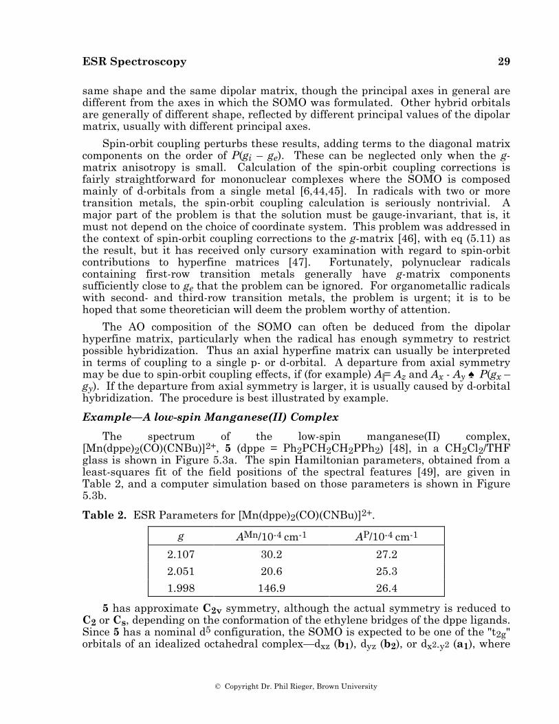
Spin-orbit coupling perturbs these results, adding terms to the diagonal matrix components on the order of P(gi – ge). These can be neglected only when the g-matrix anisotropy is small. Calculation of the spin-orbit coupling corrections is fairly straightforward for mononuclear complexes where the SOMO is composed mainly of d-orbitals from a single metal [6,44,45]. In radicals with two or more transition metals, the spin-orbit coupling calculation is seriously nontrivial. A major part of the problem is that the solution must be gauge-invariant, that is, it must not depend on the choice of coordinate system. This problem was addressed in the context of spin-orbit coupling corrections to the g-matrix [46], with eq (5.11) as the result, but it has received only cursory examination with regard to spin-orbit contributions to hyperfine matrices [47]. Fortunately, polynuclear radicals containing first-row transition metals generally have g-matrix components sufficiently close to ge that the problem can be ignored. For organometallic radicals with second- and third-row transition metals, the problem is urgent; it is to be hoped that some theoretician will deem the problem worthy of attention.

The AO composition of the SOMO can often be deduced from the dipolar hyperfine matrix, particularly when the radical has enough symmetry to restrict possible hybridization. Thus an axial hyperfine matrix can usually be interpreted in terms of coupling to a single p- or d-orbital. A departure from axial symmetry may be due to spin-orbit coupling effects, if (for example) A||= Az and Ax - Ay ♠ P(gx – gy). If the departure from axial symmetry is larger, it is usually caused by d-orbital hybridization. The procedure is best illustrated by example.

Example—A low-spin Manganese(II) Complex

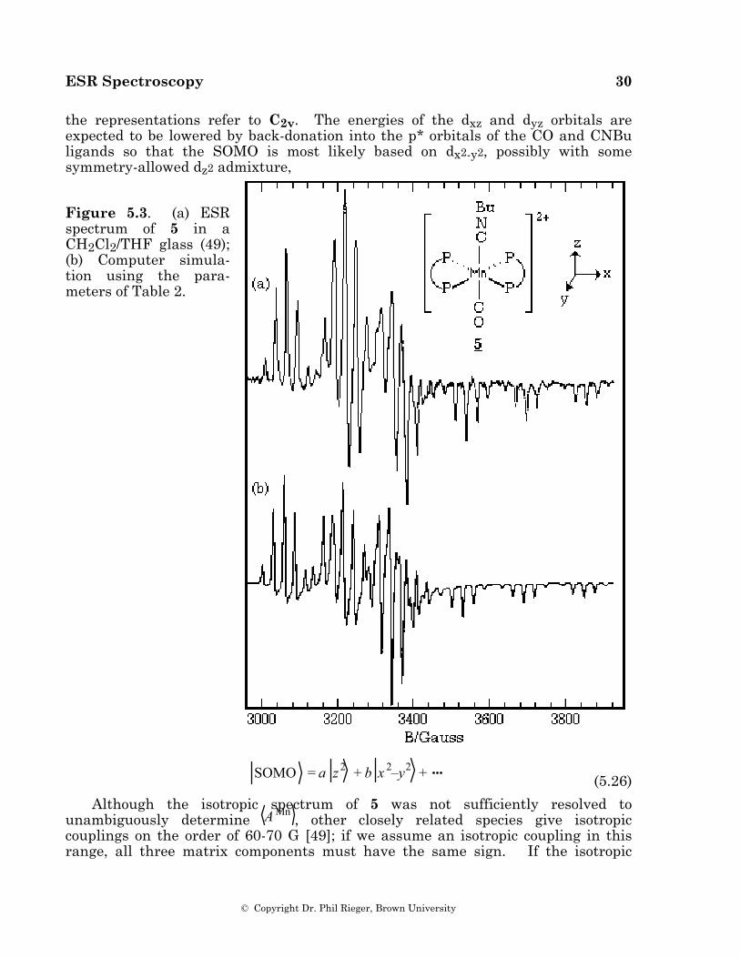
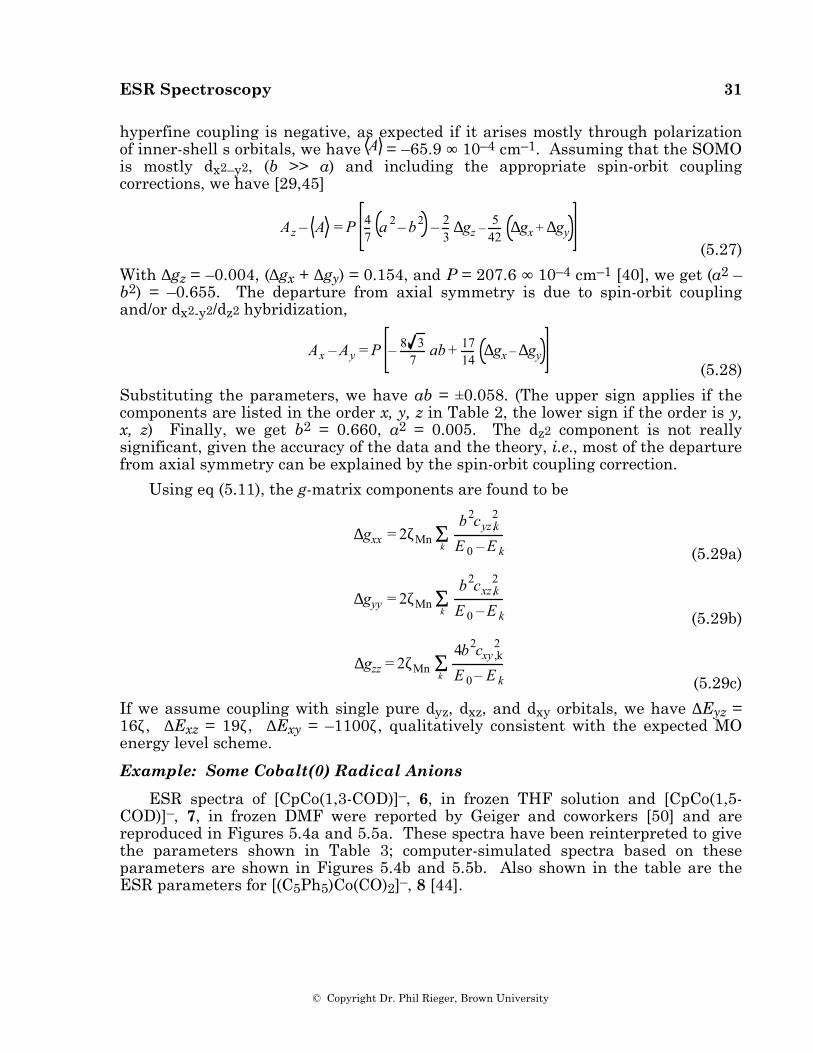
The spectrum of the low-spin manganese(II) complex, [Mn(dppe)2(CO)(CNBu)]2+, 5 (dppe = Ph2PCH2CH2PPh2) [48], in a CH2Cl2/THF glass is shown in Figure 5.3a. The spin Hamiltonian parameters, obtained from a least-squares fit of the field positions of the spectral features [49], are given in Table 2, and a computer simulation based on those parameters is shown in Figure 5.3b.

Table 2. ESR Parameters for [Mn(dppe)2(CO)(CNBu)]2+.

g AMn/10-4 cm-1 AP/10-4 cm-1

2.107 30.2 27.2

2.051 20.6 25.3

1.998 146.9 26.4

5 has approximate C2v symmetry, although the actual symmetry is reduced to C2 or Cs, depending on the conformation of the ethylene bridges of the dppe ligands. Since 5 has a nominal d5 configuration, the SOMO is expected to be one of the "t2g" orbitals of an idealized octahedral complex—dxz (b1), dyz (b2), or dx2-y2 (a1), where

ESR Spectroscopy 30


the representations refer to C2v. The energies of the dxz and dyz orbitals are expected to be lowered by back-donation into the p* orbitals of the CO and CNBu ligands so that the SOMO is most likely based on dx2-y2, possibly with some symmetry-allowed dz2 admixture,

Figure 5.3. (a) ESR spectrum of 5 in a CH2Cl2/THF glass (49); (b) Computer simula-tion using the para-meters of Table 2.

SOMO = a z 2 + b x 2–y2 + (5.26)

Although the isotropic spectrum of 5 was not sufficiently resolved to unambiguously determine A Mn

, other closely related species give isotropic couplings on the order of 60-70 G [49]; if we assume an isotropic coupling in this range, all three matrix components must have the same sign. If the isotropic

ESR Spectroscopy 31


hyperfine coupling is negative, as expected if it arises mostly through polarization of inner-shell s orbitals, we have A = –65.9 ∞ 10–4 cm–1. Assuming that the SOMO is mostly dx2–y2, (b >> a) and including the appropriate spin-orbit coupling corrections, we have [29,45]

Az – A = P 4

7a 2 – b2 – 2

3∆gz – 5

42∆gx + ∆gy

(5.27)

With ∆gz = –0.004, (∆gx + ∆gy) = 0.154, and P = 207.6 ∞ 10–4 cm–1 [40], we get (a2 – b2) = –0.655. The departure from axial symmetry is due to spin-orbit coupling and/or dx2-y2/dz2 hybridization,

Ax – Ay = P – 8 3

7ab + 17

14∆gx – ∆gy

(5.28)

Substituting the parameters, we have ab = ±0.058. (The upper sign applies if the components are listed in the order x, y, z in Table 2, the lower sign if the order is y, x, z) Finally, we get b2 = 0.660, a2 = 0.005. The dz2 component is not really significant, given the accuracy of the data and the theory, i.e., most of the departure from axial symmetry can be explained by the spin-orbit coupling correction.

Using eq (5.11), the g-matrix components are found to be

∆gxx = 2ζMn

b2cyz,k2

E 0 – E kΣ

k (5.29a)

∆gyy = 2ζMn

b2cxz,k2

E 0 – E kΣ

k (5.29b)

∆gzz = 2ζMn

4b2cxy ,k2

E 0 – E kΣk (5.29c)

If we assume coupling with single pure dyz, dxz, and dxy orbitals, we have ∆Eyz = 16ζ, ∆Exz = 19ζ, ∆Exy = –1100ζ, qualitatively consistent with the expected MO energy level scheme.

Example: Some Cobalt(0) Radical Anions

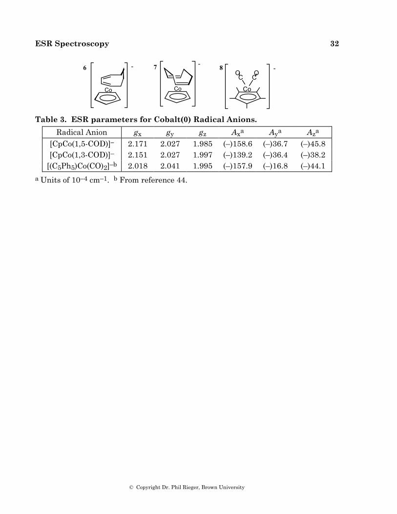
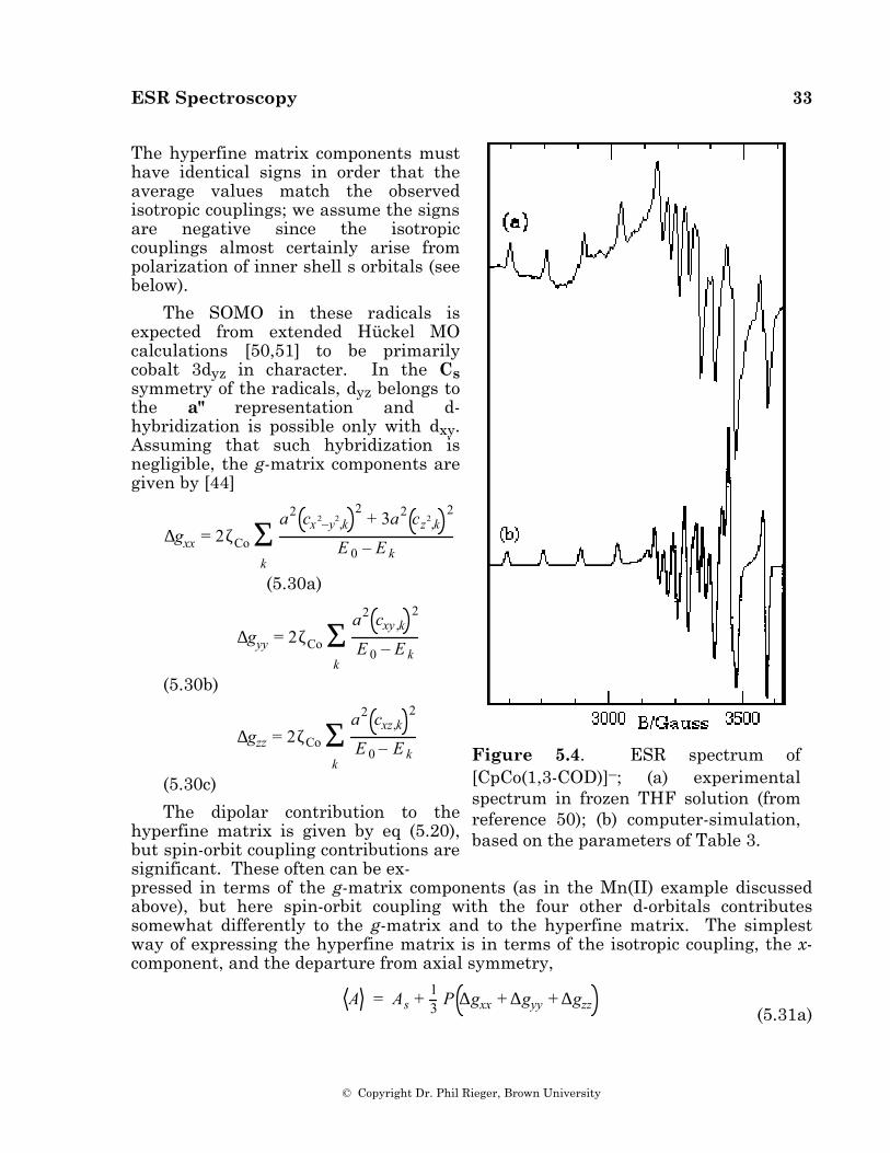
ESR spectra of [CpCo(1,3-COD)]–, 6, in frozen THF solution and [CpCo(1,5-COD)]–, 7, in frozen DMF were reported by Geiger and coworkers [50] and are reproduced in Figures 5.4a and 5.5a. These spectra have been reinterpreted to give the parameters shown in Table 3; computer-simulated spectra based on these parameters are shown in Figures 5.4b and 5.5b. Also shown in the table are the ESR parameters for [(C5Ph5)Co(CO)2]–, 8 [44].

ESR Spectroscopy 32


Co

CCOO

CoCo

- 7 86 - -

Table 3. ESR parameters for Cobalt(0) Radical Anions.

Radical Anion gx gy gz Axa Aya Aza [CpCo(1,5-COD)]– 2.171 2.027 1.985 (–)158.6 (–)36.7 (–)45.8 [CpCo(1,3-COD)]– 2.151 2.027 1.997 (–)139.2 (–)36.4 (–)38.2

[(C5Ph5)Co(CO)2]–b 2.018 2.041 1.995 (–)157.9 (–)16.8 (–)44.1

a Units of 10–4 cm–1. b From reference 44.

ESR Spectroscopy 33


The hyperfine matrix components must have identical signs in order that the average values match the observed isotropic couplings; we assume the signs are negative since the isotropic couplings almost certainly arise from polarization of inner shell s orbitals (see below).

The SOMO in these radicals is expected from extended Hückel MO calculations [50,51] to be primarily cobalt 3dyz in character. In the Cs symmetry of the radicals, dyz belongs to the a" representation and d-hybridization is possible only with dxy. Assuming that such hybridization is negligible, the g-matrix components are given by [44]

∆gxx = 2ζCo

a2 cx 2–y2,k2

+ 3a2 cz2,k2

E 0 – E kΣ

k (5.30a)

∆gyy = 2ζCo

a2 cxy ,k2

E 0 – E kΣ

k

(5.30b)

∆gzz = 2ζCo

a2 cxz,k2

E 0 – E kΣ

k

(5.30c)

The dipolar contribution to the hyperfine matrix is given by eq (5.20), but spin-orbit coupling contributions are significant. These often can be ex-

Figure 5.4. ESR spectrum of [CpCo(1,3-COD)]–; (a) experimental spectrum in frozen THF solution (from reference 50); (b) computer-simulation, based on the parameters of Table 3.

pressed in terms of the g-matrix components (as in the Mn(II) example discussed above), but here spin-orbit coupling with the four other d-orbitals contributes somewhat differently to the g-matrix and to the hyperfine matrix. The simplest way of expressing the hyperfine matrix is in terms of the isotropic coupling, the x-component, and the departure from axial symmetry,

A = As + 1

3 P ∆gxx + ∆gyy + ∆gzz (5.31a)

ESR Spectroscopy 34


Ax – A = P – 4

7 a2 + 23 ∆gxx – 5

42 (∆gyy + ∆gzz) (5.31b)

Ay – Az = 1714

P ∆gyy + ∆gzz

+6a2ζP

71

∆E x 2-y 2– 1

∆E z2

(5.31c)

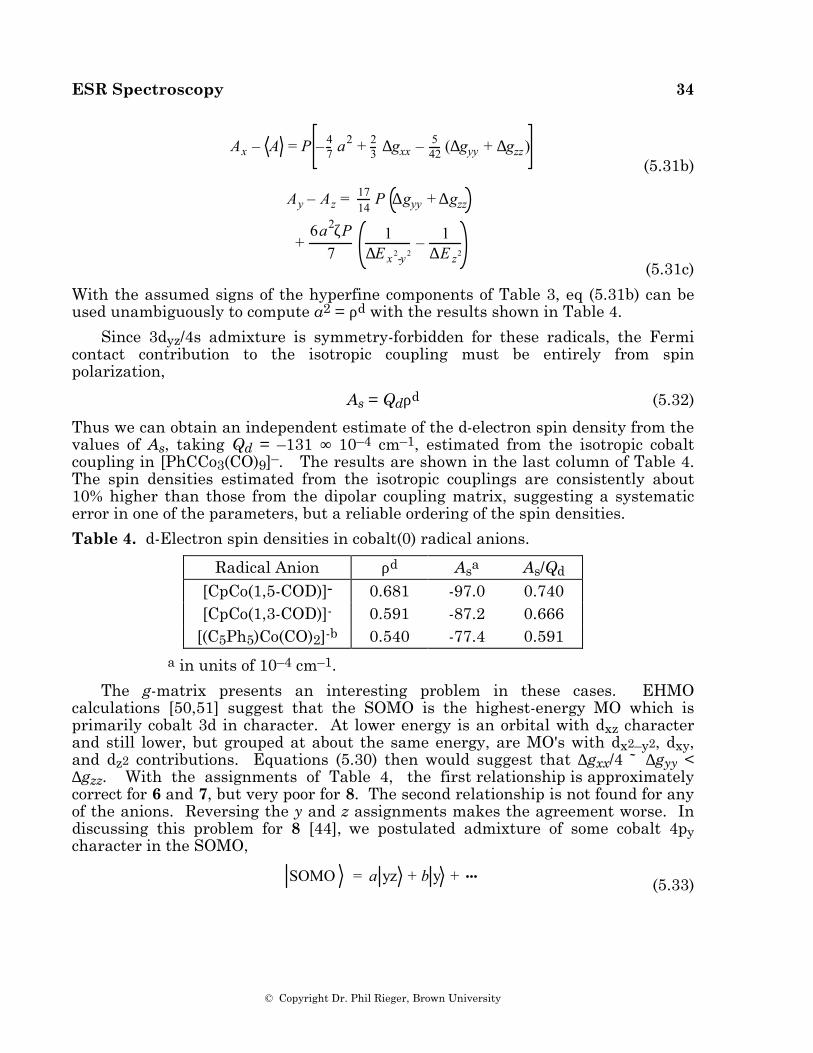
With the assumed signs of the hyperfine components of Table 3, eq (5.31b) can be used unambiguously to compute a2 = ρd with the results shown in Table 4.

Since 3dyz/4s admixture is symmetry-forbidden for these radicals, the Fermi contact contribution to the isotropic coupling must be entirely from spin polarization,

As = Qdρd (5.32)

Thus we can obtain an independent estimate of the d-electron spin density from the values of As, taking Qd = –131 ∞ 10–4 cm–1, estimated from the isotropic cobalt coupling in [PhCCo3(CO)9]–. The results are shown in the last column of Table 4. The spin densities estimated from the isotropic couplings are consistently about 10% higher than those from the dipolar coupling matrix, suggesting a systematic error in one of the parameters, but a reliable ordering of the spin densities.

Table 4. d-Electron spin densities in cobalt(0) radical anions.

Radical Anion ρd Asa As/Qd [CpCo(1,5-COD)]- 0.681 -97.0 0.740 [CpCo(1,3-COD)]- 0.591 -87.2 0.666

[(C5Ph5)Co(CO)2]-b 0.540 -77.4 0.591

a in units of 10–4 cm–1.

The g-matrix presents an interesting problem in these cases. EHMO calculations [50,51] suggest that the SOMO is the highest-energy MO which is primarily cobalt 3d in character. At lower energy is an orbital with dxz character and still lower, but grouped at about the same energy, are MO's with dx2–y2, dxy, and dz2 contributions. Equations (5.30) then would suggest that ∆gxx/4 ˜ ∆gyy < ∆gzz. With the assignments of Table 4, the first relationship is approximately correct for 6 and 7, but very poor for 8. The second relationship is not found for any of the anions. Reversing the y and z assignments makes the agreement worse. In discussing this problem for 8 [44], we postulated admixture of some cobalt 4py character in the SOMO,

SOMO = a yz + b y + (5.33)

ESR Spectroscopy 35


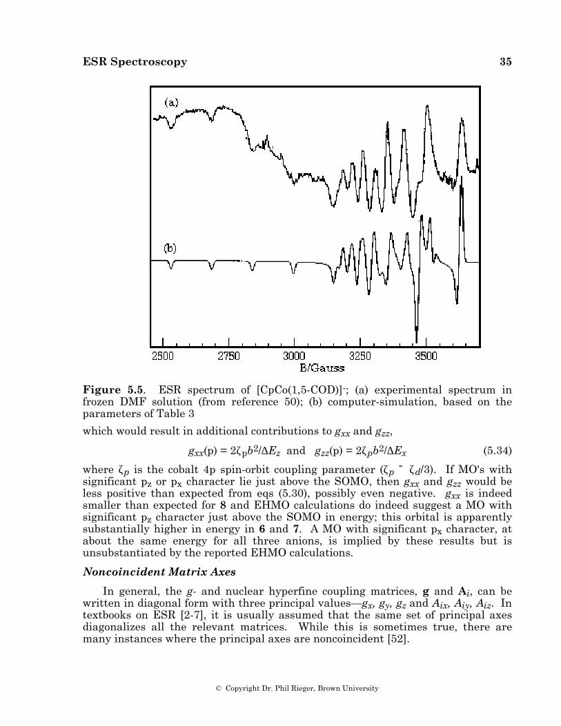
Figure 5.5. ESR spectrum of [CpCo(1,5-COD)]-; (a) experimental spectrum in frozen DMF solution (from reference 50); (b) computer-simulation, based on the parameters of Table 3

which would result in additional contributions to gxx and gzz,

gxx(p) = 2ζpb2/∆Ez and gzz(p) = 2ζpb2/∆Ex (5.34)

where ζp is the cobalt 4p spin-orbit coupling parameter (ζp ˜ ζd/3). If MO's with significant pz or px character lie just above the SOMO, then gxx and gzz would be less positive than expected from eqs (5.30), possibly even negative. gxx is indeed smaller than expected for 8 and EHMO calculations do indeed suggest a MO with significant pz character just above the SOMO in energy; this orbital is apparently substantially higher in energy in 6 and 7. A MO with significant px character, at about the same energy for all three anions, is implied by these results but is unsubstantiated by the reported EHMO calculations.

Noncoincident Matrix Axes

In general, the g- and nuclear hyperfine coupling matrices, g and Ai, can be written in diagonal form with three principal values—gx, gy, gz and Aix, Aiy, Aiz. In textbooks on ESR [2-7], it is usually assumed that the same set of principal axes diagonalizes all the relevant matrices. While this is sometimes true, there are many instances where the principal axes are noncoincident [52].

ESR Spectroscopy 36


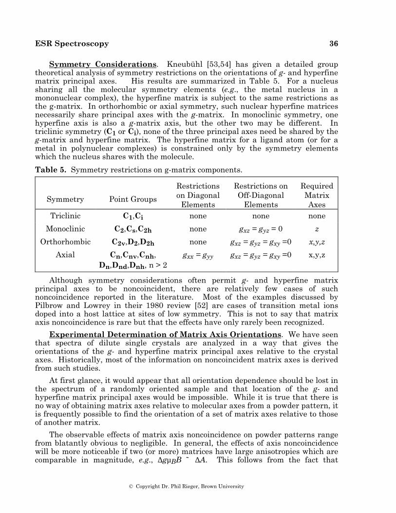
Symmetry Considerations. Kneubühl [53,54] has given a detailed group theoretical analysis of symmetry restrictions on the orientations of g- and hyperfine matrix principal axes. His results are summarized in Table 5. For a nucleus sharing all the molecular symmetry elements (e.g., the metal nucleus in a mononuclear complex), the hyperfine matrix is subject to the same restrictions as the g-matrix. In orthorhombic or axial symmetry, such nuclear hyperfine matrices necessarily share principal axes with the g-matrix. In monoclinic symmetry, one hyperfine axis is also a g-matrix axis, but the other two may be different. In triclinic symmetry (C1 or Ci), none of the three principal axes need be shared by the g-matrix and hyperfine matrix. The hyperfine matrix for a ligand atom (or for a metal in polynuclear complexes) is constrained only by the symmetry elements which the nucleus shares with the molecule.

Table 5. Symmetry restrictions on g-matrix components.

Symmetry

Point Groups

Restrictions on Diagonal

Elements

Restrictions on Off-Diagonal

Elements

Required Matrix Axes

Triclinic C1,Ci none none none

Monoclinic C2,Cs,C2h none gxz = gyz = 0 z

Orthorhombic C2v,D2,D2h none gxz = gyz = gxy =0 x,y,z

Axial Cn,Cnv,Cnh, Dn,Dnd,Dnh, n > 2

gxx = gyy gxz = gyz = gxy =0 x,y,z

Although symmetry considerations often permit g- and hyperfine matrix principal axes to be noncoincident, there are relatively few cases of such noncoincidence reported in the literature. Most of the examples discussed by Pilbrow and Lowrey in their 1980 review [52] are cases of transition metal ions doped into a host lattice at sites of low symmetry. This is not to say that matrix axis noncoincidence is rare but that the effects have only rarely been recognized.

Experimental Determination of Matrix Axis Orientations. We have seen that spectra of dilute single crystals are analyzed in a way that gives the orientations of the g- and hyperfine matrix principal axes relative to the crystal axes. Historically, most of the information on noncoincident matrix axes is derived from such studies.

At first glance, it would appear that all orientation dependence should be lost in the spectrum of a randomly oriented sample and that location of the g- and hyperfine matrix principal axes would be impossible. While it is true that there is no way of obtaining matrix axes relative to molecular axes from a powder pattern, it is frequently possible to find the orientation of a set of matrix axes relative to those of another matrix.

The observable effects of matrix axis noncoincidence on powder patterns range from blatantly obvious to negligible. In general, the effects of axis noncoincidence will be more noticeable if two (or more) matrices have large anisotropies which are comparable in magnitude, e.g., ∆gµBB ˜ ∆A. This follows from the fact that

ESR Spectroscopy 37


minimum and maximum resonant fields are determined by a competition between extrema in the angle-dependent values of g and A. Consider the case of noncoincident g- and hyperfine matrix axes. For large values of |mI|, the field extrema will be determined largely by the extrema in the effective hyperfine coupling and will occur at angles close to the hyperfine matrix axes, but for small |mI|, the extrema will be determined by extrema in the effective g-value and will correspond to angles close to the g-matrix axes. The result of such a competition is that a series of features which would be equally spaced (to first order) acquires markedly uneven spacings.

There are two corollaries stemming from this generalization. Since spin 1/2 nuclei give only two hyperfine lines, there can be no variation in spacings. Thus powder spectra cannot be analyzed to extract the orientations of hyperfine matrix axes for such important nuclei as 1H, 13C, 19F, 31P, 57Fe, and 103Rh. Secondly, since the observable effects in powder spectra depend on the magnitude of the matrix anisotropies, the principal axes of the hyperfine matrix for a nucleus with small hyperfine coupling generally cannot be located from a powder spectrum, even though the relative anisotropy may be large.

Example—Chromium Nitrosyl Complex

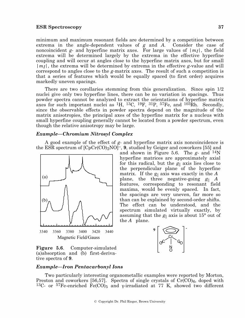
A good example of the effect of g- and hyperfine matrix axis noncoincidence is the ESR spectrum of [CpCr(CO)2NO]–, 9, studied by Geiger and coworkers [55] and

3340 3360 3380 3400 3420 3440Magnetic Field/Gauss

(a)

(b)

Figure 5.6. Computer-simulated (a)absorption and (b) first-deriva-tive spectra of 9.

and shown in Figure 5.6. The g- and 14N hyperfine matrices are approximately axial for this radical, but the g|| axis lies close to the perpendicular plane of the hyperfine matrix. If the g|| axis was exactly in the A⊥ plane, the three negative-going g|| A⊥ features, corresponding to resonant field maxima, would be evenly spaced. In fact, the spacings are very uneven, far more so than can be explained by second-order shifts. The effect can be understood, and the spectrum simulated virtually exactly, by assuming that the g|| axis is about 15° out of the A⊥ plane.

Cr

N O

CC OO

-9

Example—Iron Pentacarbonyl Ions

Two particularly interesting organometallic examples were reported by Morton, Preston and coworkers [56,57]. Spectra of single crystals of Cr(CO)6, doped with 13C- or 57Fe-enriched Fe(CO)5 and γ-irradiated at 77 K, showed two different

ESR Spectroscopy 38


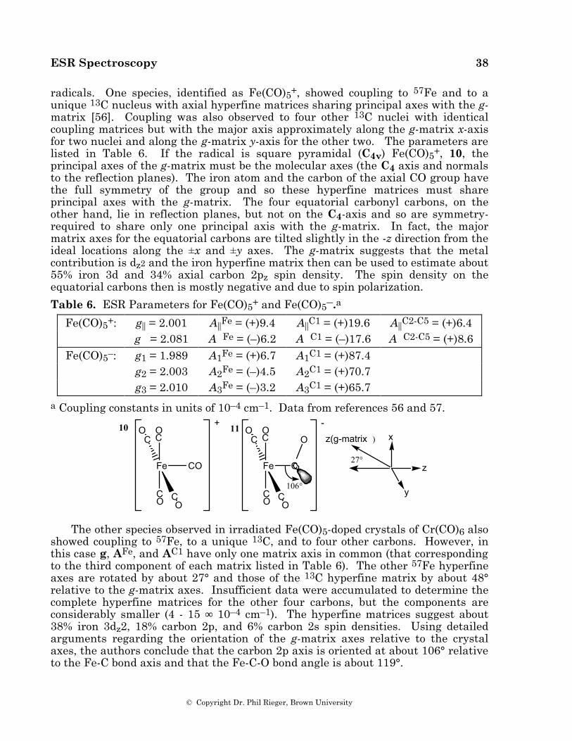
radicals. One species, identified as Fe(CO)5+, showed coupling to 57Fe and to a unique 13C nucleus with axial hyperfine matrices sharing principal axes with the g-matrix [56]. Coupling was also observed to four other 13C nuclei with identical coupling matrices but with the major axis approximately along the g-matrix x-axis for two nuclei and along the g-matrix y-axis for the other two. The parameters are listed in Table 6. If the radical is square pyramidal (C4v) Fe(CO)5+, 10, the principal axes of the g-matrix must be the molecular axes (the C4 axis and normals to the reflection planes). The iron atom and the carbon of the axial CO group have the full symmetry of the group and so these hyperfine matrices must share principal axes with the g-matrix. The four equatorial carbonyl carbons, on the other hand, lie in reflection planes, but not on the C4-axis and so are symmetry-required to share only one principal axis with the g-matrix. In fact, the major matrix axes for the equatorial carbons are tilted slightly in the -z direction from the ideal locations along the ±x and ±y axes. The g-matrix suggests that the metal contribution is dz2 and the iron hyperfine matrix then can be used to estimate about 55% iron 3d and 34% axial carbon 2pz spin density. The spin density on the equatorial carbons then is mostly negative and due to spin polarization.

Table 6. ESR Parameters for Fe(CO)5+ and Fe(CO)5–.a

Fe(CO)5+: g|| = 2.001 A||Fe = (+)9.4 A||C1 = (+)19.6 A||C2-C5 = (+)6.4 g⊥ = 2.081 A⊥Fe = (–)6.2 A⊥C1 = (–)17.6 A⊥C2-C5 = (+)8.6

Fe(CO)5–: g1 = 1.989 A1Fe = (+)6.7 A1C1 = (+)87.4 g2 = 2.003 A2Fe = (–)4.5 A2C1 = (+)70.7 g3 = 2.010 A3Fe = (–)3.2 A3C1 = (+)65.7

a Coupling constants in units of 10–4 cm–1. Data from references 56 and 57.

Fe

O C

C O

OC

C

O

O

Fe

O C

C O C

OC

CO

OC

+10 11 -x

106°

27°

y

z(g-matrix )

z

The other species observed in irradiated Fe(CO)5-doped crystals of Cr(CO)6 also showed coupling to 57Fe, to a unique 13C, and to four other carbons. However, in this case g, AFe, and AC1 have only one matrix axis in common (that corresponding to the third component of each matrix listed in Table 6). The other 57Fe hyperfine axes are rotated by about 27° and those of the 13C hyperfine matrix by about 48° relative to the g-matrix axes. Insufficient data were accumulated to determine the complete hyperfine matrices for the other four carbons, but the components are considerably smaller (4 - 15 ∞ 10–4 cm–1). The hyperfine matrices suggest about 38% iron 3dz2, 18% carbon 2p, and 6% carbon 2s spin densities. Using detailed arguments regarding the orientation of the g-matrix axes relative to the crystal axes, the authors conclude that the carbon 2p axis is oriented at about 106° relative to the Fe-C bond axis and that the Fe-C-O bond angle is about 119°.

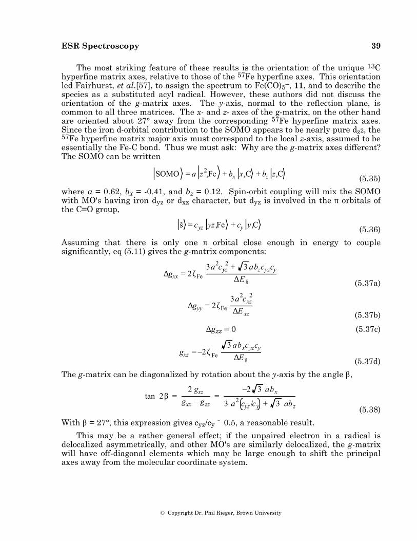
ESR Spectroscopy 39


The most striking feature of these results is the orientation of the unique 13C hyperfine matrix axes, relative to those of the 57Fe hyperfine axes. This orientation led Fairhurst, et al.[57], to assign the spectrum to Fe(CO)5–, 11, and to describe the species as a substituted acyl radical. However, these authors did not discuss the orientation of the g-matrix axes. The y-axis, normal to the reflection plane, is common to all three matrices. The x- and z- axes of the g-matrix, on the other hand are oriented about 27° away from the corresponding 57Fe hyperfine matrix axes. Since the iron d-orbital contribution to the SOMO appears to be nearly pure dz2, the 57Fe hyperfine matrix major axis must correspond to the local z-axis, assumed to be essentially the Fe-C bond. Thus we must ask: Why are the g-matrix axes different? The SOMO can be written

SOMO = a z 2,Fe + bx x,C + bz z,C (5.35)

where a = 0.62, bx = -0.41, and bz = 0.12. Spin-orbit coupling will mix the SOMO with MO's having iron dyz or dxz character, but dyz is involved in the π orbitals of the C=O group,

š = cyz yz ,Fe + cy y,C (5.36)

Assuming that there is only one π orbital close enough in energy to couple significantly, eq (5.11) gives the g-matrix components:

∆gxx = 2ζFe

3a2cyz2 + 3 abzcyzcy

∆E š (5.37a)

∆gyy = 2ζFe

3a2cxz2

∆E xz (5.37b)

∆gzz = 0 (5.37c)

gxz = –2ζFe

3 abxcyzcy

∆E š (5.37d)

The g-matrix can be diagonalized by rotation about the y-axis by the angle β,

tan 2β =

2 gxz

gxx – g zz=

–2 3 abx

3 a2 cyz /cy + 3 ab z (5.38)

With β = 27°, this expression gives cyz/cy ˜ 0.5, a reasonable result.

This may be a rather general effect; if the unpaired electron in a radical is delocalized asymmetrically, and other MO's are similarly delocalized, the g-matrix will have off-diagonal elements which may be large enough to shift the principal axes away from the molecular coordinate system.

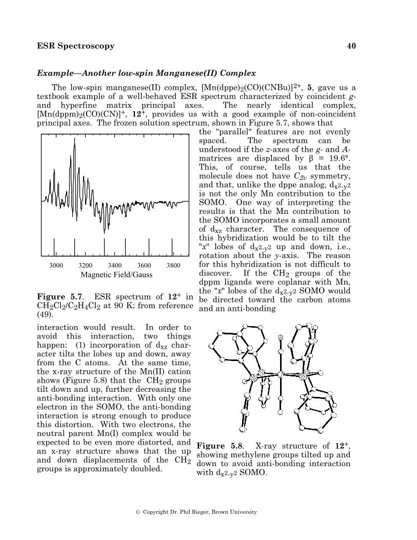
ESR Spectroscopy 40


Example—Another low-spin Manganese(II) Complex

The low-spin manganese(II) complex, [Mn(dppe)2(CO)(CNBu)]2+, 5, gave us a textbook example of a well-behaved ESR spectrum characterized by coincident g- and hyperfine matrix principal axes. The nearly identical complex, [Mn(dppm)2(CO)(CN)]+, 12+, provides us with a good example of non-coincident principal axes. The frozen solution spectrum, shown in Figure 5.7, shows that

3000 3200 3400 3600 3800Magnetic Field/Gauss

Figure 5.7. ESR spectrum of 12+ in CH2Cl2/C2H4Cl2 at 90 K; from reference (49).

the "parallel" features are not evenly spaced. The spectrum can be understood if the z-axes of the g- and A-matrices are displaced by β = 19.6°. This, of course, tells us that the molecule does not have C2v symmetry, and that, unlike the dppe analog, dx2-y2 is not the only Mn contribution to the SOMO. One way of interpreting the results is that the Mn contribution to the SOMO incorporates a small amount of dxz character. The consequence of this hybridization would be to tilt the "x" lobes of dx2-y2 up and down, i.e., rotation about the y-axis. The reason for this hybridization is not difficult to discover. If the CH2 groups of the dppm ligands were coplanar with Mn, the "x" lobes of the dx2-y2 SOMO would be directed toward the carbon atoms and an anti-bonding

interaction would result. In order to avoid this interaction, two things happen: (1) incorporation of dxz char-acter tilts the lobes up and down, away from the C atoms. At the same time, the x-ray structure of the Mn(II) cation shows (Figure 5.8) that the CH2 groups tilt down and up, further decreasing the anti-bonding interaction. With only one electron in the SOMO, the anti-bonding interaction is strong enough to produce this distortion. With two electrons, the neutral parent Mn(I) complex would be expected to be even more distorted, and an x-ray structure shows that the up and down displacements of the CH2 groups is approximately doubled.

Figure 5.8. X-ray structure of 12+, showing methylene groups tilted up and down to avoid anti-bonding interaction with dx2-y2 SOMO.

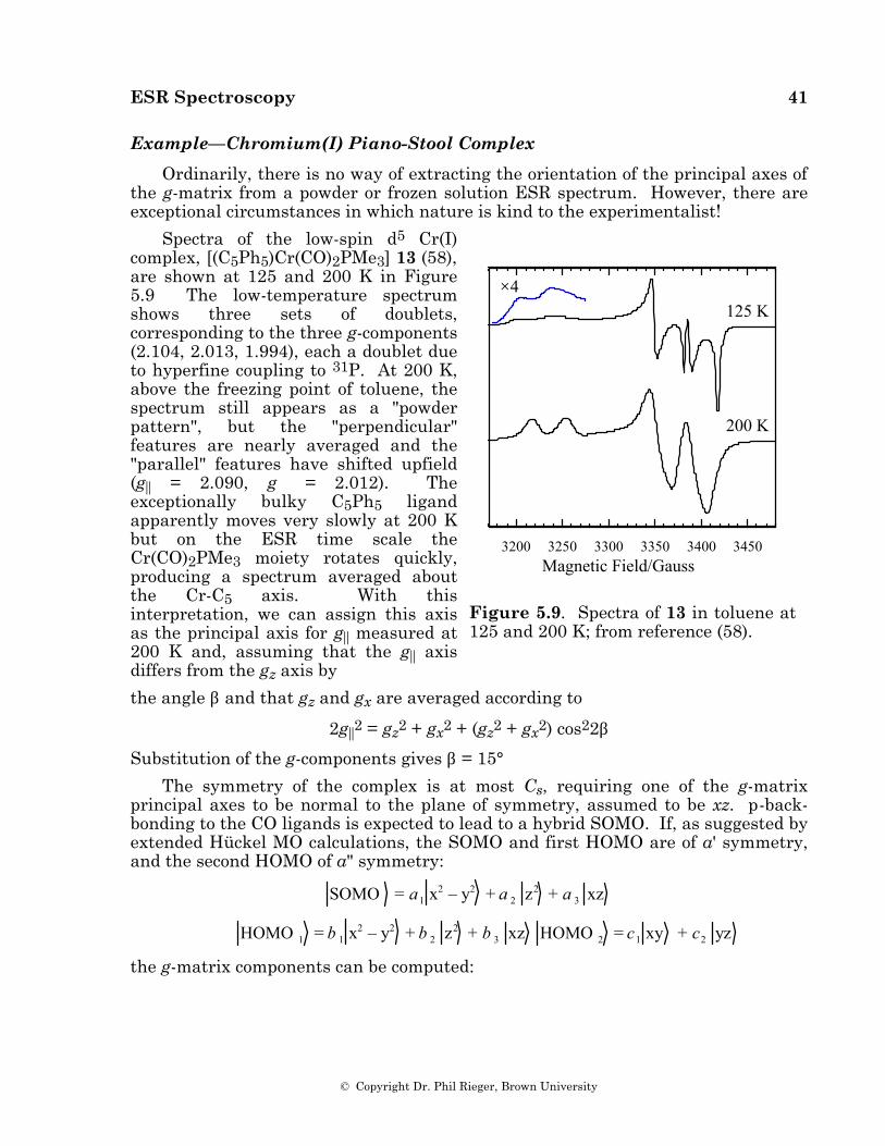
ESR Spectroscopy 41


Example—Chromium(I) Piano-Stool Complex

Ordinarily, there is no way of extracting the orientation of the principal axes of the g-matrix from a powder or frozen solution ESR spectrum. However, there are exceptional circumstances in which nature is kind to the experimentalist!

Spectra of the low-spin d5 Cr(I) complex, [(C5Ph5)Cr(CO)2PMe3] 13 (58), are shown at 125 and 200 K in Figure 5.9 The low-temperature spectrum shows three sets of doublets, corresponding to the three g-components (2.104, 2.013, 1.994), each a doublet due to hyperfine coupling to 31P. At 200 K, above the freezing point of toluene, the spectrum still appears as a "powder pattern", but the "perpendicular" features are nearly averaged and the "parallel" features have shifted upfield (g|| = 2.090, g⊥ = 2.012). The exceptionally bulky C5Ph5 ligand apparently moves very slowly at 200 K but on the ESR time scale the Cr(CO)2PMe3 moiety rotates quickly, producing a spectrum averaged about the Cr-C5 axis. With this interpretation, we can assign this axis as the principal axis for g|| measured at 200 K and, assuming that the g|| axis differs from the gz axis by


125 K

200 K

×4

Figure 5.9. Spectra of 13 in toluene at 125 and 200 K; from reference (58).

the angle β and that gz and gx are averaged according to

2g||2 = gz2 + gx2 + (gz2 + gx2) cos22β

Substitution of the g-components gives β = 15°

The symmetry of the complex is at most Cs, requiring one of the g-matrix principal axes to be normal to the plane of symmetry, assumed to be xz. p-back-bonding to the CO ligands is expected to lead to a hybrid SOMO. If, as suggested by extended Hückel MO calculations, the SOMO and first HOMO are of a' symmetry, and the second HOMO of a" symmetry:

SOMO = a1 x2 – y2 + a 2 z2 + a 3 xz

HOMO 1 = b 1 x2 – y2 + b 2 z2 + b 3 xz HOMO 2 = c1 xy + c2 yz

the g-matrix components can be computed:

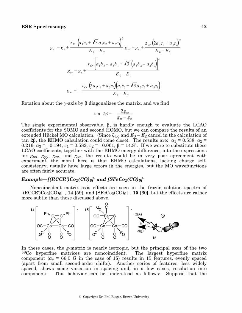
ESR Spectroscopy 42


g xx = g e +ζCr a 1c2 + 3 a 2c2 + a 3c1

2

E 0 – E 2

g zz = g e +

ζCr 2a 1c1 + a 3c2

2

E 0 – E 2

g yy = g e +ζCr a 1b 3 – a3b 1 + 3 a 3b 2 – a2b 3

2

E 0 – E 1

g xz = –ζCr 2a1c1 + a 3c2 a1c2 + 3 a 2c2 + a 3c1

E 0 – E 2

Rotation about the y-axis by β diagonalizes the matrix, and we find

tan 2β = – 2g xz

g zz – gxx The single experimental observable, β, is hardly enough to evaluate the LCAO coefficients for the SOMO and second HOMO, but we can compare the results of an extended Hückel MO calculation. (Since ζCo and E0 – E2 cancel in the calculation of tan 2β, the EHMO calculation could come close). The results are: a1 = 0.538, a2 = 0.216, a3 = –0.194, c1 = 0.582, c2 = –0.061, β = 14.8°. If we were to substitute these LCAO coefficients, together with the EHMO energy difference, into the expressions for gxx, gyy, gzz, and gxz, the results would be in very poor agreement with experiment; the moral here is that EHMO calculations, lacking charge self-consistency, usually have large errors in the energies, but the MO wavefunctions are often fairly accurate.

Example—[(RCCR')Co2(CO)6]- and [SFeCo2(CO)9]-

Noncoincident matrix axis effects are seen in the frozen solution spectra of [(RCCR')Co2(CO)6]–, 14 [59], and [SFeCo2(CO)9]–, 15 [60], but the effects are rather more subtle than those discussed above.

Co Co

Fe SPh

CO

C O

C O

OC

O C

OC

C

CC OO

Co Co

C C Ph

CO

C O

C O

OC Co CoCC OO

O

y

b

16

14 15- -

z(g)

z(A)

In these cases, the g-matrix is nearly isotropic, but the principal axes of the two 59Co hyperfine matrices are noncoincident. The largest hyperfine matrix component (ay = 66.0 G in the case of 15) results in 15 features, evenly spaced (apart from small second-order shifts). Another series of features, less widely spaced, shows some variation in spacing and, in a few cases, resolution into components. This behavior can be understood as follows: Suppose that the

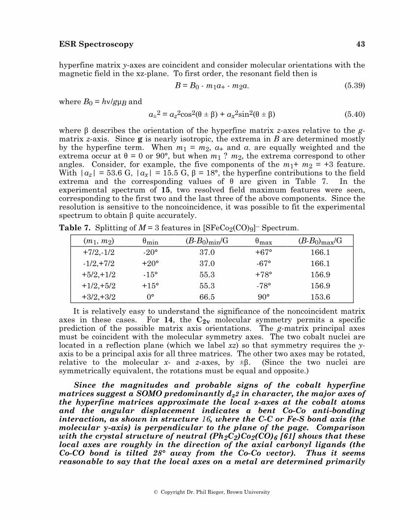
ESR Spectroscopy 43


hyperfine matrix y-axes are coincident and consider molecular orientations with the magnetic field in the xz-plane. To first order, the resonant field then is B = B0 - m1a+ - m2a- (5.39)

where B0 = hν/gµB and

a±2 = az2cos2(θ ± β) + ax2sin2(θ ± β) (5.40)

where β describes the orientation of the hyperfine matrix z-axes relative to the g-matrix z-axis. Since g is nearly isotropic, the extrema in B are determined mostly by the hyperfine term. When m1 = m2, a+ and a- are equally weighted and the extrema occur at θ = 0 or 90°, but when m1 ? m2, the extrema correspond to other angles. Consider, for example, the five components of the m1+ m2 = +3 feature. With |az| = 53.6 G, |ax| = 15.5 G, β = 18°, the hyperfine contributions to the field extrema and the corresponding values of θ are given in Table 7. In the experimental spectrum of 15, two resolved field maximum features were seen, corresponding to the first two and the last three of the above components. Since the resolution is sensitive to the noncoincidence, it was possible to fit the experimental spectrum to obtain β quite accurately.

Table 7. Splitting of M = 3 features in [SFeCo2(CO)9]– Spectrum.

(m1, m2) θmin (B-B0)min/G θmax (B-B0)max/G +7/2,-1/2 -20° 37.0 +67° 166.1 -1/2,+7/2 +20° 37.0 -67° 166.1 +5/2,+1/2 -15° 55.3 +78° 156.9 +1/2,+5/2 +15° 55.3 -78° 156.9 +3/2,+3/2 0° 66.5 90° 153.6

It is relatively easy to understand the significance of the noncoincident matrix axes in these cases. For 14, the C2v molecular symmetry permits a specific prediction of the possible matrix axis orientations. The g-matrix principal axes must be coincident with the molecular symmetry axes. The two cobalt nuclei are located in a reflection plane (which we label xz) so that symmetry requires the y-axis to be a principal axis for all three matrices. The other two axes may be rotated, relative to the molecular x- and z-axes, by ±β. (Since the two nuclei are symmetrically equivalent, the rotations must be equal and opposite.)

Since the magnitudes and probable signs of the cobalt hyperfine matrices suggest a SOMO predominantly dz2 in character, the major axes of the hyperfine matrices approximate the local z-axes at the cobalt atoms and the angular displacement indicates a bent Co-Co anti-bonding interaction, as shown in structure 16, where the C-C or Fe-S bond axis (the molecular y-axis) is perpendicular to the plane of the page. Comparison with the crystal structure of neutral (Ph2C2)Co2(CO)6 [61] shows that these local axes are roughly in the direction of the axial carbonyl ligands (the Co-CO bond is tilted 28° away from the Co-Co vector). Thus it seems reasonable to say that the local axes on a metal are determined primarily

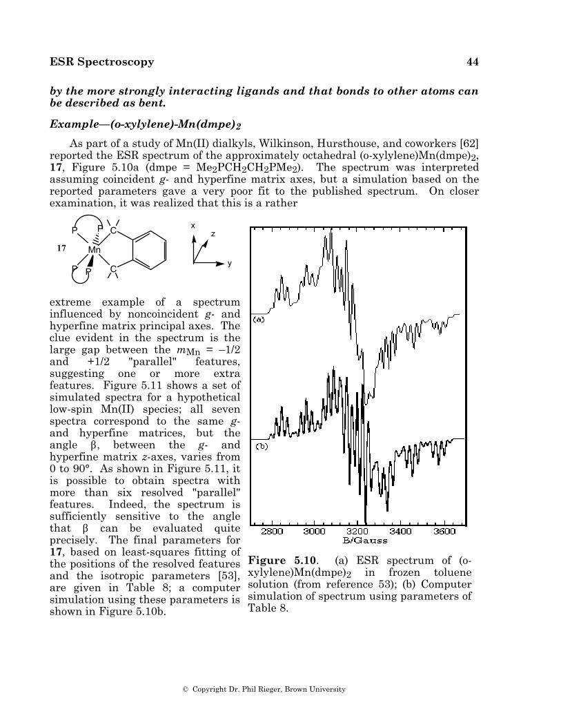
ESR Spectroscopy 44


by the more strongly interacting ligands and that bonds to other atoms can be described as bent.

Example—(o-xylylene)-Mn(dmpe)2

As part of a study of Mn(II) dialkyls, Wilkinson, Hursthouse, and coworkers [62] reported the ESR spectrum of the approximately octahedral (o-xylylene)Mn(dmpe)2, 17, Figure 5.10a (dmpe = Me2PCH2CH2PMe2). The spectrum was interpreted assuming coincident g- and hyperfine matrix axes, but a simulation based on the reported parameters gave a very poor fit to the published spectrum. On closer examination, it was realized that this is a rather

Mn

C

CP

P

P

P

xz

y

17

extreme example of a spectrum influenced by noncoincident g- and hyperfine matrix principal axes. The clue evident in the spectrum is the large gap between the mMn = –1/2 and +1/2 "parallel" features, suggesting one or more extra features. Figure 5.11 shows a set of simulated spectra for a hypothetical low-spin Mn(II) species; all seven spectra correspond to the same g- and hyperfine matrices, but the angle β, between the g- and hyperfine matrix z-axes, varies from 0 to 90°. As shown in Figure 5.11, it is possible to obtain spectra with more than six resolved "parallel" features. Indeed, the spectrum is sufficiently sensitive to the angle that β can be evaluated quite precisely. The final parameters for 17, based on least-squares fitting of the positions of the resolved features and the isotropic parameters [53], are given in Table 8; a computer simulation using these parameters is shown in Figure 5.10b.

Figure 5.10. (a) ESR spectrum of (o-xylylene)Mn(dmpe)2 in frozen toluene solution (from reference 53); (b) Computer simulation of spectrum using parameters of Table 8.

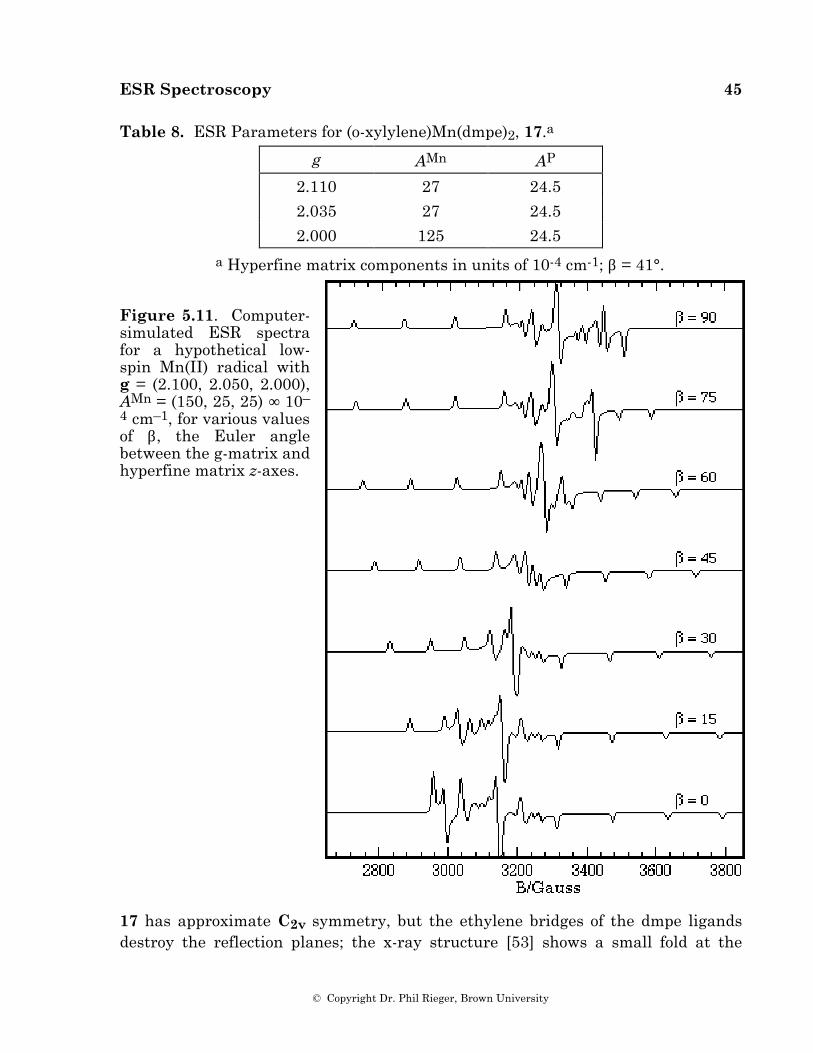
ESR Spectroscopy 45


Table 8. ESR Parameters for (o-xylylene)Mn(dmpe)2, 17.a

g AMn AP

2.110 27 24.5

2.035 27 24.5

2.000 125 24.5

a Hyperfine matrix components in units of 10-4 cm-1; β = 41°.

Figure 5.11. Computer-simulated ESR spectra for a hypothetical low-spin Mn(II) radical with g = (2.100, 2.050, 2.000), AMn = (150, 25, 25) ∞ 10–4 cm–1, for various values of β, the Euler angle between the g-matrix and hyperfine matrix z-axes.

17 has approximate C2v symmetry, but the ethylene bridges of the dmpe ligands destroy the reflection planes; the x-ray structure [53] shows a small fold at the

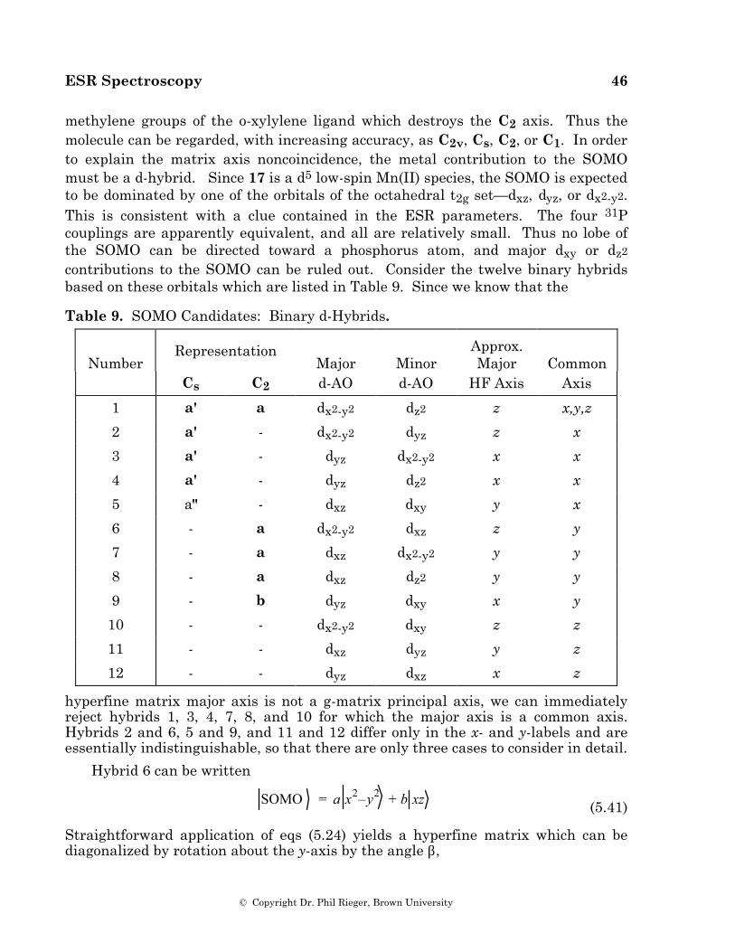
ESR Spectroscopy 46


methylene groups of the o-xylylene ligand which destroys the C2 axis. Thus the molecule can be regarded, with increasing accuracy, as C2v, Cs, C2, or C1. In order to explain the matrix axis noncoincidence, the metal contribution to the SOMO must be a d-hybrid. Since 17 is a d5 low-spin Mn(II) species, the SOMO is expected to be dominated by one of the orbitals of the octahedral t2g set—dxz, dyz, or dx2-y2. This is consistent with a clue contained in the ESR parameters. The four 31P couplings are apparently equivalent, and all are relatively small. Thus no lobe of the SOMO can be directed toward a phosphorus atom, and major dxy or dz2 contributions to the SOMO can be ruled out. Consider the twelve binary hybrids based on these orbitals which are listed in Table 9. Since we know that the

Table 9. SOMO Candidates: Binary d-Hybrids.

Number

Representation Major

Minor

Approx. Major

Common

Cs C2 d-AO d-AO HF Axis Axis

1 a' a dx2-y2 dz2 z x,y,z

2 a' - dx2-y2 dyz z x

3 a' - dyz dx2-y2 x x

4 a' - dyz dz2 x x

5 a" - dxz dxy y x

6 - a dx2-y2 dxz z y

7 - a dxz dx2-y2 y y

8 - a dxz dz2 y y

9 - b dyz dxy x y

10 - - dx2-y2 dxy z z

11 - - dxz dyz y z

12 - - dyz dxz x z

hyperfine matrix major axis is not a g-matrix principal axis, we can immediately reject hybrids 1, 3, 4, 7, 8, and 10 for which the major axis is a common axis. Hybrids 2 and 6, 5 and 9, and 11 and 12 differ only in the x- and y-labels and are essentially indistinguishable, so that there are only three cases to consider in detail.

Hybrid 6 can be written

SOMO = a x2–y2 + b xz (5.41)

Straightforward application of eqs (5.24) yields a hyperfine matrix which can be diagonalized by rotation about the y-axis by the angle β,

ESR Spectroscopy 47


tan 2β = –2b/a (5.42)

The g-matrix can be written in relatively simple form if we assume that the only MO's close enough in energy to contribute significantly are the filled MO's, primarily dxz and dyz in character. With this assumption, we obtain a matrix which can be diagonalized by rotation about the y-axis by β',

tan 2β' = – 2b/a

1 – b /a 2 (5.43)

For reasonable values of the hybridization ratio, b/a up to about 0.5, β and β' can differ by only a few degrees and this kind of hybrid cannot explain the matrix axis noncoincidence. Following the same reasoning with x and y interchanged, exactly the same conclusions can be reached for hybrid 2.

Hybrids 11 and 12 are

SOMO = a xz + b yz (5.44)

In this case, the hyperfine matrix remains axial, independent of the hybridization ratio, although the principal axes are rotated in the xy-plane by an angle α equal to angle β of eq (5.43). Assuming that only MO's with predominantly dxz, dyz, or dx2–y2 character contribute, a g-matrix is found which can be diagonalized by rotation in the xy-plane by the angle α', also given by eq (5.43). Thus this hybrid gives identical g- and hyperfine matrix principal axes for all hybridization ratios.

Finally, hybrid 9,

SOMO = a yz + b xy (5.45)

gives an axial hyperfine matrix with principal axes rotated in the xz-plane by an angle β, given by eq (5.43). The g-matrix is somewhat more complicated,

∆g = 2ζ

acx2–y22

∆E x 2–y2+

bcxz2

∆E xz0 -

2ab cx2 –y22

∆E x 2–y2–

ab cxz2

∆E xz

0bcyz

2

∆E yz0

–2ab cx2–y2

2

∆E x2–y 2–

ab cxz2

∆E xz0

2bcx2–y22

∆Ex 2–y 2+

acxz2

∆E xz

(5.46)

Diagonalization requires rotation about the y-axis by the angle β',

ESR Spectroscopy 48


tan 2β' = – 2b

a2Q + 1

Q – 1 – b/a2

4Q – 1 (5.47)

where

Q =cx 2–y2

2

∆E x 2–y2

cxz2

∆Exz

cx 2–y22

∆E x 2–y2

cxz2

∆Exz (5.48)

Since the energy differences, ∆Ex2–y2 and ∆Exz are expected to be comparable, the parameter Q is probably not far from unity. For Q = 1, eq (5.47) has a particularly simple form, tan 2β' = +2a/b so that, for small b/a, we expect β ˜ 0 and β' ˜ 45°, entirely consistent with experiment. The axial hyperfine matrix is in agreement with experiment, and the principal values of the g-matrix can also be rationalized with reasonable values of Q and b/a. A small rotation of dyz about the y-axis might reflect the small displacements of the phosphorus atoms from the idealized octahedral positions.

An extended Hückel MO calculation on 15 supports the assumptions made in the above analysis in that the three "t2g" orbitals are indeed close together in energy and remain nearly nonbonding metal-based d-orbitals. The detailed agreement is less satisfactory: the SOMO is predicted to be primarily dx2–y2 with a small dxz admixture (hybrid 6 of Table 9), a result which can be ruled out from our analysis of the ESR results. The EHMO overlap matrix based on the x-ray structure suggests that the molecule is much closer to C2 symmetry than to Cs. If we accept that conclusion, then dxz/dxy hybridization is less likely than dyz/dxy, as we tacitly assumed above.

We considered several alternative explanations for the matrix axis noncoincidence in 15. In particular, it seemed possible that delocalization of spin density into the o-xylylene ligand, either through the σ-bonds or into the π-system, might lead to significant contributions to the off-diagonal terms of the g-matrix. While the EHMO calculations suggest that the MO's containing dx2–y2 and dyz do have contributions from the carbon atoms of the o-xylylene group, the amount is far too small to rationalize rotation of the g-matrix axes by 41°; indeed, to explain the effect in this way would require each of several carbon atoms to contribute 5% or more to the MO's with dx2–y2 or dyz character, unreasonably large considering the poor overlap of these metal d-orbitals with the relevant carbon orbitals.

6. Molecules with More than One Unpaired Electron

Molecules with two or more unpaired electrons may be divided into two classes: By far the most common examples are molecules where the unpaired electrons are contained in a set of degenerate atomic or molecular orbitals with qualitatively similar spatial distributions, e.g., an octahedral Cr(III) (4A2g) or Ni(II) (3A2g) complex, or a triplet state molecule like O2, or the excited triplet states of naphthalene or benzophenone.

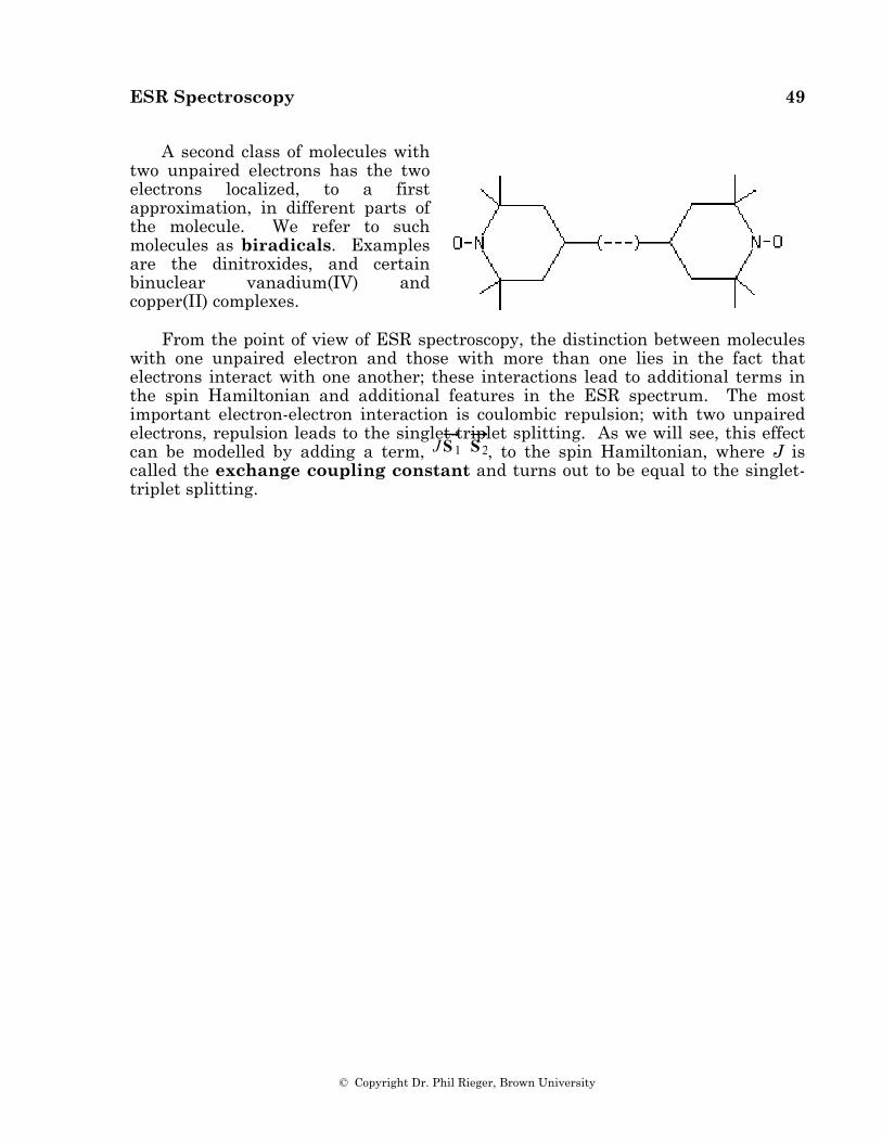
ESR Spectroscopy 49


A second class of molecules with two unpaired electrons has the two electrons localized, to a first approximation, in different parts of the molecule. We refer to such molecules as biradicals. Examples are the dinitroxides, and certain binuclear vanadium(IV) and copper(II) complexes.

From the point of view of ESR spectroscopy, the distinction between molecules with one unpaired electron and those with more than one lies in the fact that electrons interact with one another; these interactions lead to additional terms in the spin Hamiltonian and additional features in the ESR spectrum. The most important electron-electron interaction is coulombic repulsion; with two unpaired electrons, repulsion leads to the singlet-triplet splitting. As we will see, this effect can be modelled by adding a term, J S 1⋅ S 2, to the spin Hamiltonian, where J is called the exchange coupling constant and turns out to be equal to the singlet-triplet splitting.

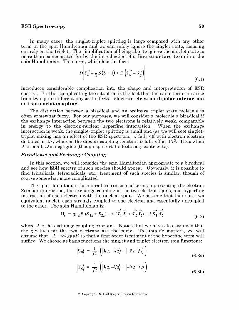
ESR Spectroscopy 50


In many cases, the singlet-triplet splitting is large compared with any other term in the spin Hamiltonian and we can safely ignore the singlet state, focusing entirely on the triplet. The simplification of being able to ignore the singlet state is more than compensated for by the introduction of a fine structure term into the spin Hamiltonian. This term, which has the form

D S z

2 – 13 S S + 1 + E S x

2 – S y2

(6.1)

introduces considerable complication into the shape and interpretation of ESR spectra. Further complicating the situation is the fact that the same term can arise from two quite different physical effects: electron-electron dipolar interaction and spin-orbit coupling.

The distinction between a biradical and an ordinary triplet state molecule is often somewhat fuzzy. For our purposes, we will consider a molecule a biradical if the exchange interaction between the two electrons is relatively weak, comparable in energy to the electron-nuclear hyperfine interaction. When the exchange interaction is weak, the singlet-triplet splitting is small and (as we will see) singlet-triplet mixing has an effect of the ESR spectrum. J falls off with electron-electron distance as 1/r, whereas the dipolar coupling constant D falls off as 1/r3. Thus when J is small, D is negligible (though spin-orbit effects may contribute).

Biradicals and Exchange Coupling In this section, we will consider the spin Hamiltonian appropriate to a biradical and see how ESR spectra of such species should appear. Obviously, it is possible to find triradicals, tetraradicals, etc.; treatment of such species is similar, though of course somewhat more complicated.

The spin Hamiltonian for a biradical consists of terms representing the electron Zeeman interaction, the exchange coupling of the two electron spins, and hyperfine interaction of each electron with the nuclear spins. We assume that there are two equivalent nuclei, each strongly coupled to one electron and essentially uncoupled to the other. The spin Hamiltonian is:

Hs = gµBB (S 1z + S 2z) + A (S 1⋅I1 + S 2⋅I2) + J S1⋅S 2 (6.2)

where J is the exchange coupling constant. Notice that we have also assumed that the g-values for the two electrons are the same. To simplify matters, we will assume that |A| << gµBB so that a first-order treatment of the hyperfine term will suffice. We choose as basis functions the singlet and triplet electron spin functions:

S 0 = 1

21 21 2, –1 21 2 – –1 21 2 , 1 21 2

(6.3a)

T 0 = 1

21 21 2, –1 21 2 + –1 21 2 , 1 21 2

(6.3b)

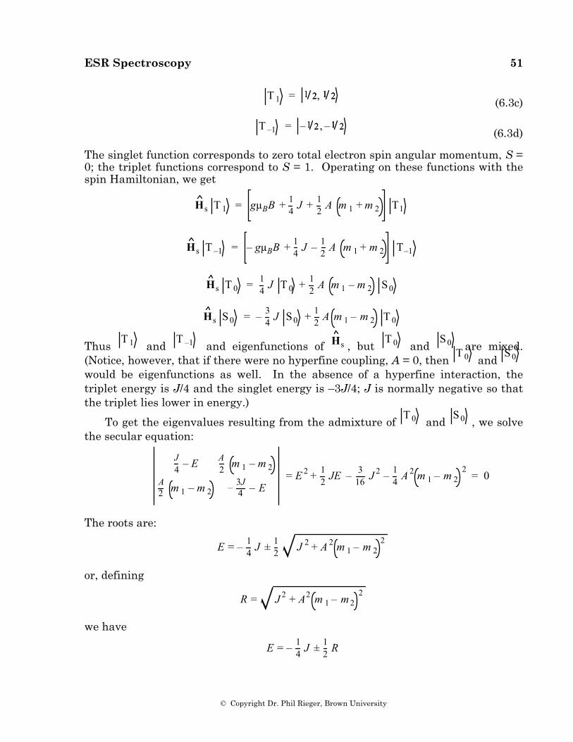
ESR Spectroscopy 51


T 1 = 1 21 2, 1 21 2

(6.3c)

T –1 = –1 21 2 , –1 21 2

(6.3d)

The singlet function corresponds to zero total electron spin angular momentum, S = 0; the triplet functions correspond to S = 1. Operating on these functions with the spin Hamiltonian, we get

Hs T 1 = gµBB + 1

4 J + 12 A m 1 + m 2 T1

Hs T –1 = – gµBB + 1

4 J – 12 A m 1 + m 2 T–1

Hs T 0 = 1

4 J T 0 + 12 A m 1 – m 2 S0

Hs S 0 = – 3

4 J S0 + 12 A m 1 – m 2 T 0

Thus T 1 and

T –1 and eigenfunctions of Hs , but

T 0 and S 0 are mixed.

(Notice, however, that if there were no hyperfine coupling, A = 0, then T 0 and

S 0 would be eigenfunctions as well. In the absence of a hyperfine interaction, the triplet energy is J/4 and the singlet energy is –3J/4; J is normally negative so that the triplet lies lower in energy.)

To get the eigenvalues resulting from the admixture of T 0 and

S 0 , we solve the secular equation:

J4 – E A

2 m 1 – m 2

A2 m 1 – m 2 – 3J

4 – E= E 2 + 1

2 JE – 316 J 2 – 1

4 A 2 m 1 – m 22

= 0

The roots are:

E = – 14 J ± 1

2 J 2 + A 2 m 1 – m 22

or, defining

R = J 2 + A2 m 1 – m 22

we have

E = – 1

4 J ± 12 R

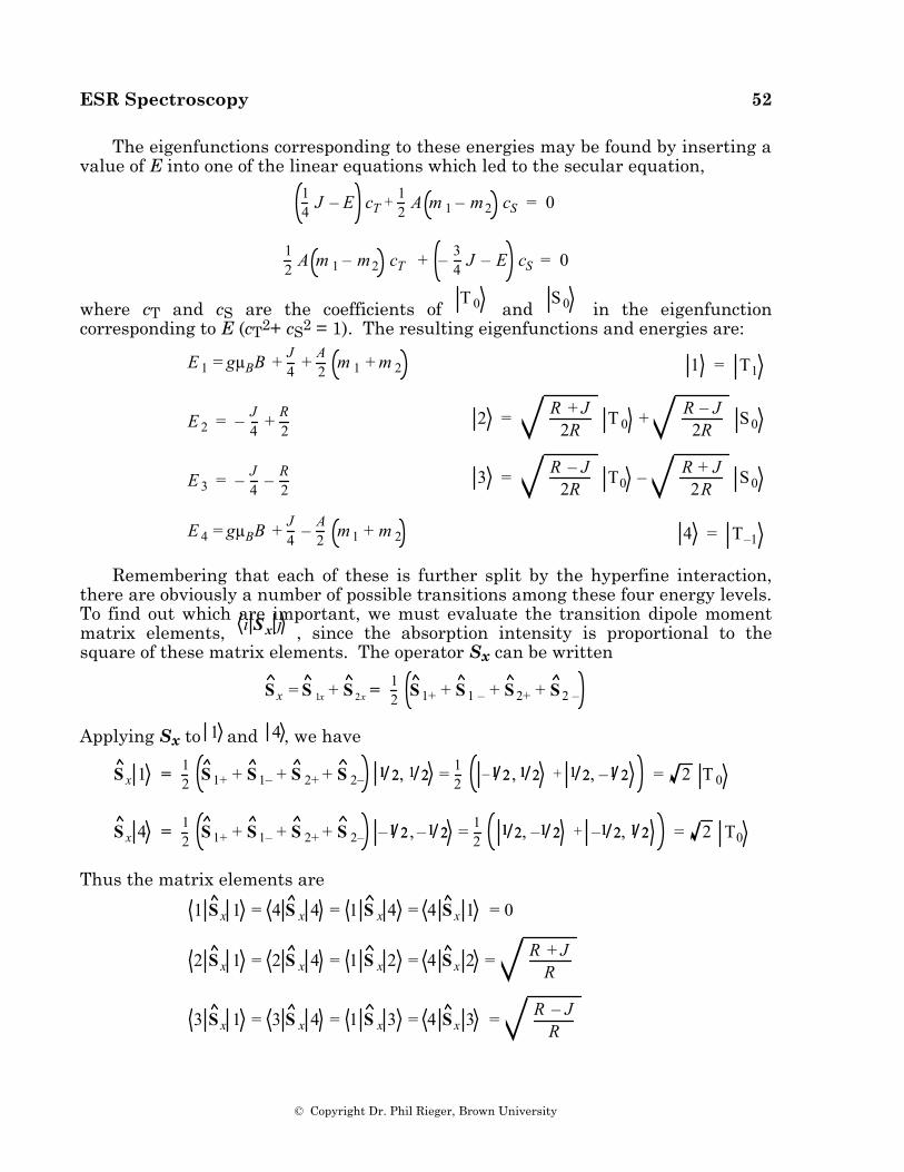
ESR Spectroscopy 52


The eigenfunctions corresponding to these energies may be found by inserting a value of E into one of the linear equations which led to the secular equation,

14 J – E cT + 1

2 A m 1 – m2 cS = 0

12 A m 1 – m2 cT + – 3

4 J – E cS = 0

where cT and cS are the coefficients of T 0 and

S 0 in the eigenfunction corresponding to E (cT2+ cS2 = 1). The resulting eigenfunctions and energies are:

E 1 = gµBB + J

4 + A2 m 1 + m 2

1 = T1

E 2 = – J

4 + R2

2 = R + J

2RT 0 + R – J

2RS0

E 3 = – J

4 – R2

3 = R – J

2RT0 – R + J

2RS0

E 4 = gµBB + J

4 – A2 m 1 + m 2

4 = T–1

Remembering that each of these is further split by the hyperfine interaction, there are obviously a number of possible transitions among these four energy levels. To find out which are important, we must evaluate the transition dipole moment matrix elements,

i S x j , since the absorption intensity is proportional to the square of these matrix elements. The operator Sx can be written

S x = S 1x + S 2x = 1

2 S 1+ + S 1 – + S 2+ + S 2 –

Applying Sx to 1 and 4 , we have

S x 1 = 1

2 S 1+ + S 1– + S 2+ + S 2– 1 21 2, 1 21 2 = 12

–1 21 2 , 1 21 2 + 1 21 2, –1 21 2 = 2 T 0

S x 4 = 1

2 S 1+ + S 1– + S 2+ + S 2– –1 21 2 , –1 21 2 = 12

1 21 2, –1 21 2 + –1 21 2, 1 21 2 = 2 T0

Thus the matrix elements are

1 S x 1 = 4 S x 4 = 1 S x 4 = 4 S x 1 = 0

2 S x 1 = 2 S x 4 = 1 S x 2 = 4 S x 2 = R + J

R

3 S x 1 = 3 S x 4 = 1 S x 3 = 4 S x 3 = R – J

R

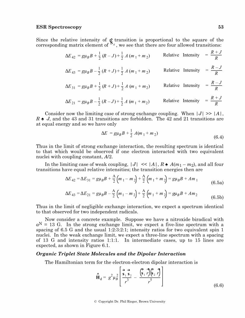
ESR Spectroscopy 53


Since the relative intensity of a transition is proportional to the square of the corresponding matrix element of

S x , we see that there are four allowed transitions:

∆E 42 = gµB B + 1

2 (R – J ) + 12 A (m 1 + m 2)

Relative Intensity = R + JR

∆E 43 = gµB B – 1

2 (R + J ) + 12 A (m 1 + m 2)

Relative Intensity = R – JR

∆E 31 = gµB B + 1

2 (R + J ) + 12 A (m 1 + m2)

Relative Intensity = R – JR

∆E 21 = gµB B – 1

2 (R – J ) + 12 A (m 1 + m2)

Relative Intensity = R + JR

Consider now the limiting case of strong exchange coupling. When |J| >> |A|, R ♠ J, and the 43 and 31 transitions are forbidden. The 42 and 21 transitions are at equal energy and so we have only

∆E = gµB B + 1

2 A(m 1 + m 2) (6.4)

Thus in the limit of strong exchange interaction, the resulting spectrum is identical to that which would be observed if one electron interacted with two equivalent nuclei with coupling constant, A/2.

In the limiting case of weak coupling, |J| << |A|, R ♠ A(m1 – m2), and all four transitions have equal relative intensities; the transition energies then are

∆E 42 = ∆E31 = gµBB + A

2 m 1 – m 2 + A2 m 1 + m 2 = gµBB + Am 1 (6.5a)

∆E 43 = ∆E21 = gµBB – A

2 m 1 – m 2 + A2 m 1 + m 2 = gµB B + Am2 (6.5b)

Thus in the limit of negligible exchange interaction, we expect a spectrum identical to that observed for two independent radicals.

Now consider a concrete example. Suppose we have a nitroxide biradical with aN = 13 G. In the strong exchange limit, we expect a five-line spectrum with a spacing of 6.5 G and the usual 1:2:3:2:1; intensity ratios for two equivalent spin 1 nuclei. In the weak exchange limit, we expect a three-line spectrum with a spacing of 13 G and intensity ratios 1:1:1. In intermediate cases, up to 15 lines are expected, as shown in Figure 6.1.

Organic Triplet State Molecules and the Dipolar Interaction The Hamiltonian term for the electron-electron dipolar interaction is

Hd = g2µB2 s 1⋅s 2

r3 –s 1⋅r s 2⋅r

r5

(6.6)

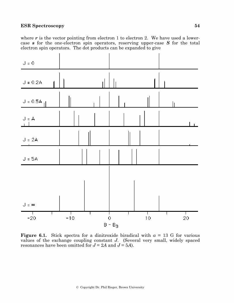
ESR Spectroscopy 54


where r is the vector pointing from electron 1 to electron 2. We have used a lower-case s for the one-electron spin operators, reserving upper-case S for the total electron spin operators. The dot products can be expanded to give

Figure 6.1. Stick spectra for a dinitroxide biradical with a = 13 G for various values of the exchange coupling constant J. (Several very small, widely spaced resonances have been omitted for J = 2A and J = 5A).

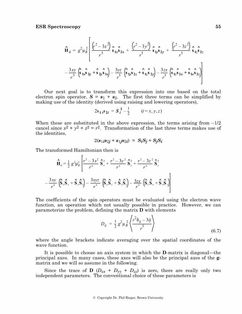
ESR Spectroscopy 55


H d = g2µB2 r 2 – 3x 2

r 5s 1xs 2x +

r2 – 3y2

r5s 1ys 2y +

r2 – 3z 2

r5s 1zs 2z

– 3xy

r 5s 1xs 2y + s 2ys 1x – 3yz

r5s 1ys 2z + s 1zs 2y – 3zx

r5s 1zs 2x + s 1xs 2z

Our next goal is to transform this expression into one based on the total electron spin operator, S = s1 + s2. The first three terms can be simplified by making use of the identity (derived using raising and lowering operators),

2s 1 is 2i = S i

2 – 12 (i = x, y, z )

When these are substituted in the above expression, the terms arising from –1/2 cancel since x2 + y2 + z2 = r2. Transformation of the last three terms makes use of the identities, 2(s1is2j + s1js2i) = SiSj + SjSi

The transformed Hamiltonian then is

Hd = 1

2 g2µB2 r 2 – 3x2

r 5S x

2+ r 2 – 3y 2

r 5S z

2+ r 2 – 3z 2

r 5S z

2

–3xyr 5 S xS y + S yS x –

3xyzr 5 S yS z + S z S y – 3zx

r 5 S z S x + S xS z

The coefficients of the spin operators must be evaluated using the electron wave function, an operation which not usually possible in practice. However, we can parameterize the problem, defining the matrix D with elements

Dij = 1

2 g2µB2 r2δij – 3ij

r5 (6.7)

where the angle brackets indicate averaging over the spatial coordinates of the wave function.

It is possible to choose an axis system in which the D-matrix is diagonal—the principal axes. In many cases, these axes will also be the principal axes of the g-matrix and we will so assume in the following.

Since the trace of D (Dxx + Dyy + Dzz) is zero, there are really only two independent parameters. The conventional choice of these parameters is

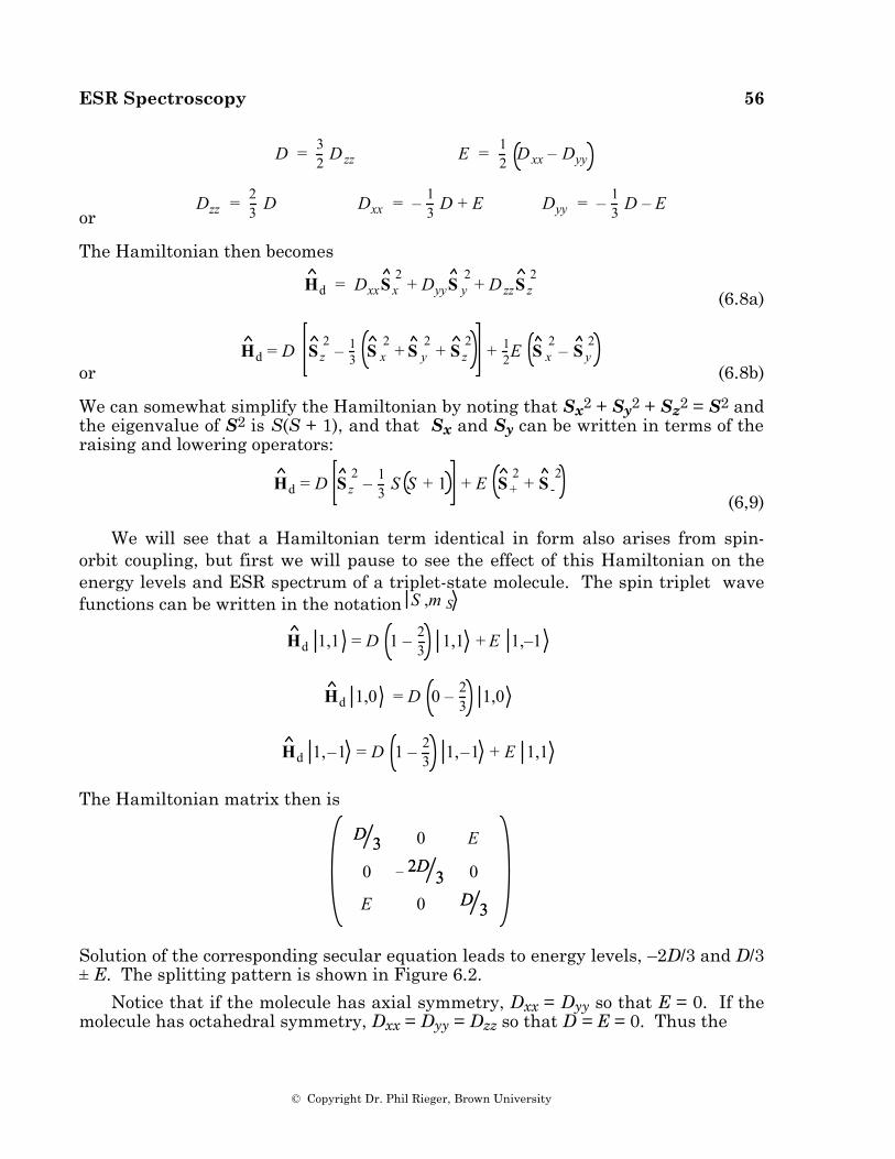
ESR Spectroscopy 56


D = 3

2 D zz E = 1

2 D xx – Dyy

or Dzz = 2

3 D

Dxx = – 13 D + E

Dyy = – 1

3 D – E

The Hamiltonian then becomes

Hd = DxxS x

2+ DyyS y

2+ D zzS z

2

(6.8a)

or

Hd = D S z

2– 1

3 S x2

+ S y2

+ S z2

+ 12E S x

2– S y

2

(6.8b)

We can somewhat simplify the Hamiltonian by noting that Sx2 + Sy2 + Sz2 = S2 and the eigenvalue of S2 is S(S + 1), and that Sx and Sy can be written in terms of the raising and lowering operators:

Hd = D S z

2– 1

3 S S + 1 + E S +2

+ S -2

(6,9)

We will see that a Hamiltonian term identical in form also arises from spin-orbit coupling, but first we will pause to see the effect of this Hamiltonian on the energy levels and ESR spectrum of a triplet-state molecule. The spin triplet wave functions can be written in the notation S ,m S

Hd 1,1 = D 1 – 23 1,1 + E 1,–1

Hd 1,0 = D 0 – 23 1,0

Hd 1,–1 = D 1 – 23 1,–1 + E 1,1

The Hamiltonian matrix then is

D 3D 3 0 E

0 – 2D3

2D3 0

E 0 D 3D 3

Solution of the corresponding secular equation leads to energy levels, –2D/3 and D/3 ± E. The splitting pattern is shown in Figure 6.2.

Notice that if the molecule has axial symmetry, Dxx = Dyy so that E = 0. If the molecule has octahedral symmetry, Dxx = Dyy = Dzz so that D = E = 0. Thus the

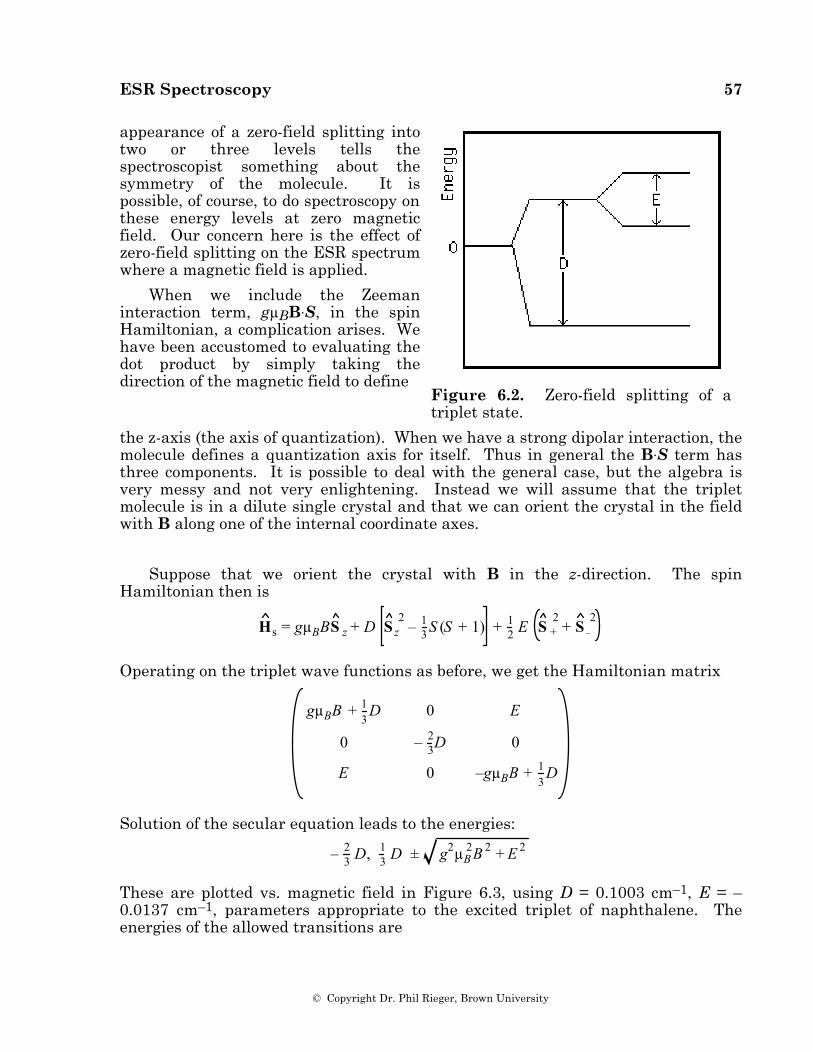
ESR Spectroscopy 57


appearance of a zero-field splitting into two or three levels tells the spectroscopist something about the symmetry of the molecule. It is possible, of course, to do spectroscopy on these energy levels at zero magnetic field. Our concern here is the effect of zero-field splitting on the ESR spectrum where a magnetic field is applied.

When we include the Zeeman interaction term, gµBB.S, in the spin Hamiltonian, a complication arises. We have been accustomed to evaluating the dot product by simply taking the direction of the magnetic field to define

Figure 6.2. Zero-field splitting of a triplet state.

the z-axis (the axis of quantization). When we have a strong dipolar interaction, the molecule defines a quantization axis for itself. Thus in general the B.S term has three components. It is possible to deal with the general case, but the algebra is very messy and not very enlightening. Instead we will assume that the triplet molecule is in a dilute single crystal and that we can orient the crystal in the field with B along one of the internal coordinate axes.

Suppose that we orient the crystal with B in the z-direction. The spin Hamiltonian then is

Hs = gµBBS z + D S z

2– 1

3 S (S + 1) + 12 E S +

2+ S –

2

Operating on the triplet wave functions as before, we get the Hamiltonian matrix

gµBB + 1

3D 0 E

0 – 23D 0

E 0 –gµBB + 13

D

Solution of the secular equation leads to the energies:

– 23 D, 1

3 D ± g2µB2B 2 + E 2

These are plotted vs. magnetic field in Figure 6.3, using D = 0.1003 cm–1, E = –0.0137 cm–1, parameters appropriate to the excited triplet of naphthalene. The energies of the allowed transitions are

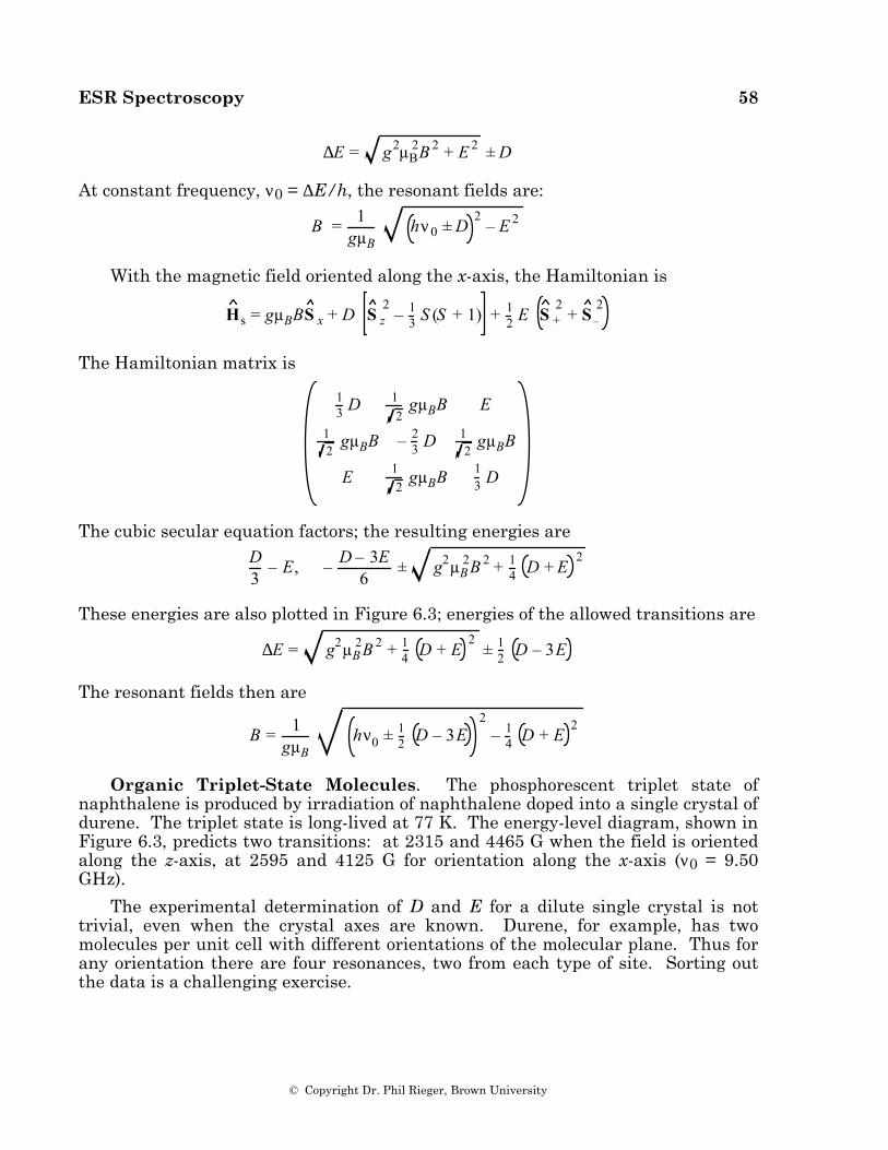
ESR Spectroscopy 58


∆E = g2µB

2B 2 + E 2 ± D

At constant frequency, ν0 = ∆E/h, the resonant fields are:

B = 1gµB

hν0 ± D2

– E 2

With the magnetic field oriented along the x-axis, the Hamiltonian is

Hs = gµBBS x + D S z

2– 1

3 S (S + 1) + 12 E S +

2+ S –

2

The Hamiltonian matrix is

13 D 1

2gµBB E

12

gµBB – 23 D 1

2gµBB

E 12

gµBB 13 D

The cubic secular equation factors; the resulting energies are

D3

– E, – D – 3E6

± g2µB2B 2 + 1

4 D + E2

These energies are also plotted in Figure 6.3; energies of the allowed transitions are

∆E = g2µB

2B 2 + 14 D + E

2± 1

2 D – 3E

The resonant fields then are

B = 1

gµBhν0 ± 1

2 D – 3E2

– 14 D + E

2

Organic Triplet-State Molecules. The phosphorescent triplet state of naphthalene is produced by irradiation of naphthalene doped into a single crystal of durene. The triplet state is long-lived at 77 K. The energy-level diagram, shown in Figure 6.3, predicts two transitions: at 2315 and 4465 G when the field is oriented along the z-axis, at 2595 and 4125 G for orientation along the x-axis (ν0 = 9.50 GHz).

The experimental determination of D and E for a dilute single crystal is not trivial, even when the crystal axes are known. Durene, for example, has two molecules per unit cell with different orientations of the molecular plane. Thus for any orientation there are four resonances, two from each type of site. Sorting out the data is a challenging exercise.

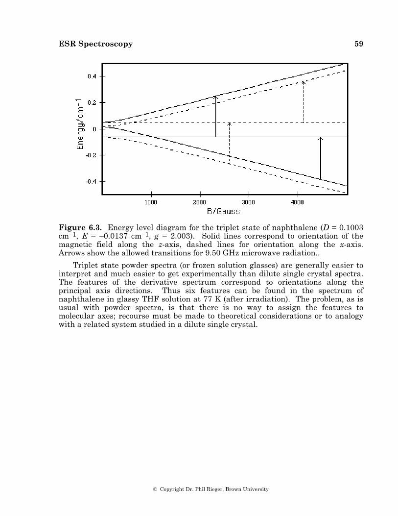
ESR Spectroscopy 59


Figure 6.3. Energy level diagram for the triplet state of naphthalene (D = 0.1003 cm–1, E = –0.0137 cm–1, g = 2.003). Solid lines correspond to orientation of the magnetic field along the z-axis, dashed lines for orientation along the x-axis. Arrows show the allowed transitions for 9.50 GHz microwave radiation..

Triplet state powder spectra (or frozen solution glasses) are generally easier to interpret and much easier to get experimentally than dilute single crystal spectra. The features of the derivative spectrum correspond to orientations along the principal axis directions. Thus six features can be found in the spectrum of naphthalene in glassy THF solution at 77 K (after irradiation). The problem, as is usual with powder spectra, is that there is no way to assign the features to molecular axes; recourse must be made to theoretical considerations or to analogy with a related system studied in a dilute single crystal.

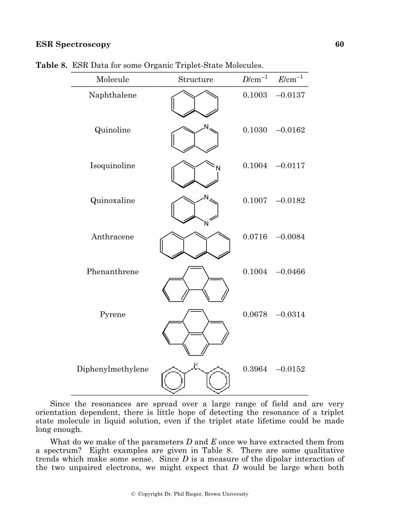
ESR Spectroscopy 60


Table 8. ESR Data for some Organic Triplet-State Molecules.

Molecule Structure D/cm–1 E/cm–1

Naphthalene

0.1003 –0.0137

Quinoline N

0.1030 –0.0162

Isoquinoline N

0.1004 –0.0117

Quinoxaline

N

N

0.1007 –0.0182

Anthracene

0.0716 –0.0084

Phenanthrene

0.1004 –0.0466

Pyrene

0.0678 –0.0314

Diphenylmethylene

0.3964 –0.0152

Since the resonances are spread over a large range of field and are very orientation dependent, there is little hope of detecting the resonance of a triplet state molecule in liquid solution, even if the triplet state lifetime could be made long enough.

What do we make of the parameters D and E once we have extracted them from a spectrum? Eight examples are given in Table 8. There are some qualitative trends which make some sense. Since D is a measure of the dipolar interaction of the two unpaired electrons, we might expect that D would be large when both

ESR Spectroscopy 61


electrons are forced to be close together and diphenylmethylene does indeed give the largest value of D. When the p-system remains about the same size but heteroatoms are substituted, we might expect that D would not change by much and we see that naphthalene and related nitrogen heterocyclics do indeed have nearly the same values of D. When the p-system gets bigger, we might expect D to decrease and anthracene and pyrene fulfill this expectation, but phenanthrene seems anomalous. To go beyond a qualitative explanation of D or to explain E at all requires rather sophisticated valence theory calculations. Indeed electron dipolar interaction parameters provide one of the more challenging test of a valence theory method.

Spin-Orbit Coupling and Transition Metal Complexes

We now will show that spin-orbit coupling can give a spin Hamiltonian term identical to that which we obtained from the electron dipolar interaction. Consider the spin Hamiltonian including orbital angular momentum and the usual spin-orbit coupling term:

Hs = µBB⋅ L + geS + λL ⋅S

(6.10)

where λ is the spin-orbit coupling constant. The zero-order ground state wave function will be characterized by the quantum numbers, L, mL, S, mS, and we assume that the wave function is orbitally nondegenerate, i.e., mL = 0. Thus we write the ground state wave function as m L ,m S = 0,m S . With B defining the z-axis, the energy is easily found to first order in perturbation theory

E (1) = gµBB m S (6.11)

since Lz 0,m S = 0. The second-order energy is not so simple since the excited states in general have nonzero mL. Thus we get second-order contributions from matrix elements connecting 0,m S with excited state functions:

E (2) = –

0,mS ,0 µBB + λS ⋅L + geµBB⋅S m L ,i,m S ,i

2

E i(1) – E 0

(1)•i (6.12)

The matrix element can be expanded and written as

m S ,0 µBB + λS m S,i 0 L mL ,i + geµBB ⋅ m S,0 S m S ,i 0 m L ,i

Since the orbital functions , 0 and m L ,i , are orthogonal, the second term vanishes. The absolute value square of the matrix element of a Hermitean operator can be written as

i Op j

2= i Op j j Op i

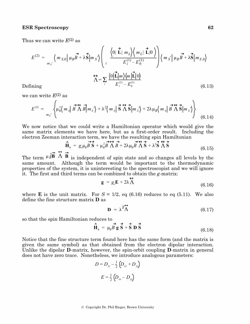
ESR Spectroscopy 62


Thus we can write E(2) as

E (2) = m S,0 µBB + λS m S ′ ⋅0| L | mL mL | L |0

E i(1) – E 0

(1)•i

⋅ m S′ µB B + λS mS ,0•m S ′

Defining

Λ =

0 L m m L 0

E i(1) – E0

(1)Σi (6.13)

we can write E(2) as

E (2) = µB

2 m S B ⋅Λ⋅B m S ′ + λ2 m S S ⋅Λ⋅S m S′ + 2λµB m S B ⋅Λ⋅S m S ′•mS ′ (6.14)

We now notice that we could write a Hamiltonian operator which would give the same matrix elements we have here, but as a first-order result. Including the electron Zeeman interaction term, we have the resulting spin Hamiltonian

Hs = geµBB⋅S + µB

2B⋅Λ⋅B + 2λµBB ⋅Λ⋅S + λ2S ⋅Λ⋅S (6.15)

The term µB 2B ⋅ Λ⋅ B is independent of spin state and so changes all levels by the

same amount. Although the term would be important to the thermodynamic properties of the system, it is uninteresting to the spectroscopist and we will ignore it. The first and third terms can be combined to obtain the g-matrix:

g = geE + 2λΛ (6.16)

where E is the unit matrix. For S = 1/2, eq (6.16) reduces to eq (5.11). We also define the fine structure matrix D as

D = λ2Λ (6.17)

so that the spin Hamiltonian reduces to

Hs = µBB ⋅g ⋅S + S ⋅D⋅S (6.18)

Notice that the fine structure term found here has the same form (and the matrix is given the same symbol) as that obtained from the electron dipolar interaction. Unlike the dipolar D-matrix, however, the spin-orbit coupling D-matrix in general does not have zero trace. Nonetheless, we introduce analogous parameters:

D = Dzz – 1

2 Dxx + D yy

E = 1

2 Dxx – Dyy

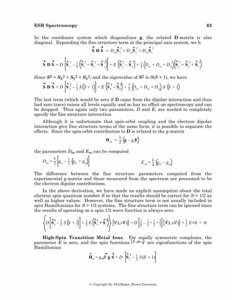
ESR Spectroscopy 63


In the coordinate system which diagonalizes g, the related D-matrix is also diagonal. Expanding the fine structure term in the principal axis system, we h

S ⋅D⋅S = D xxS x

2+ D yyS y

2+ D zzS z

2

S ⋅D⋅S = D S z

2– 1

3 S x

2+ S y

2+ S z

2+ E S x

2– S y

2+ 1

3 Dxx + Dyy + Dzz S x

2+ S y

2+ S z

2

Since S2 = Sx2 + Sy2 + Sz2, and the eigenvalue of S2 is S(S + 1), we have

S ⋅D⋅S = D S z

2– 1

3 S S + 1 + E S x

2– S y

2+ 1

3 Dxx + Dyy + D zz S S + 1

The last term (which would be zero if D came from the dipolar interaction and thus had zero trace) raises all levels equally and so has no effect on spectroscopy and can be dropped. Thus again only two parameters, D and E, are needed to completely specify the fine structure interaction.

Although it is unfortunate that spin-orbit coupling and the electron dipolar interaction give fine structure terms of the same form, it is possible to separate the effects. Since the spin-orbit contribution to D is related to the g-matrix

D so = λ

2 g – geE

the parameters Dso and Eso can be computed

Dso =

λ2 gzz – 1

2 gxx + gyy

E so = λ4 gxx – gyy

The difference between the fine structure parameters computed from the experimental g-matrix and those measured from the spectrum are presumed to be the electron dipolar contributions.

In the above derivation, we have made no explicit assumption about the total electron spin quantum number S so that the results should be correct for S = 1/2 as well as higher values. However, the fine structure term is not usually included in spin Hamiltonians for S = 1/2 systems. The fine structure term can be ignored since the results of operating on a spin 1/2 wave function is always zero:

D S z

2– 1

3 S S + 1 + 12 E S +

2+ S –

2 1 21 2,±1 21 2 = D 14 – 1

3× 1

2× 3

21 21 2 ,±1 21 2 + 1

2 E×0 = 0

High-Spin Transition Metal Ions. For axially symmetric complexes, the parameter E is zero, and the spin functions S ,m S are eigenfunctions of the spin Hamiltonian

Hs = µBB ⋅g ⋅S + D S z

2– 1

3 S (S + 1)

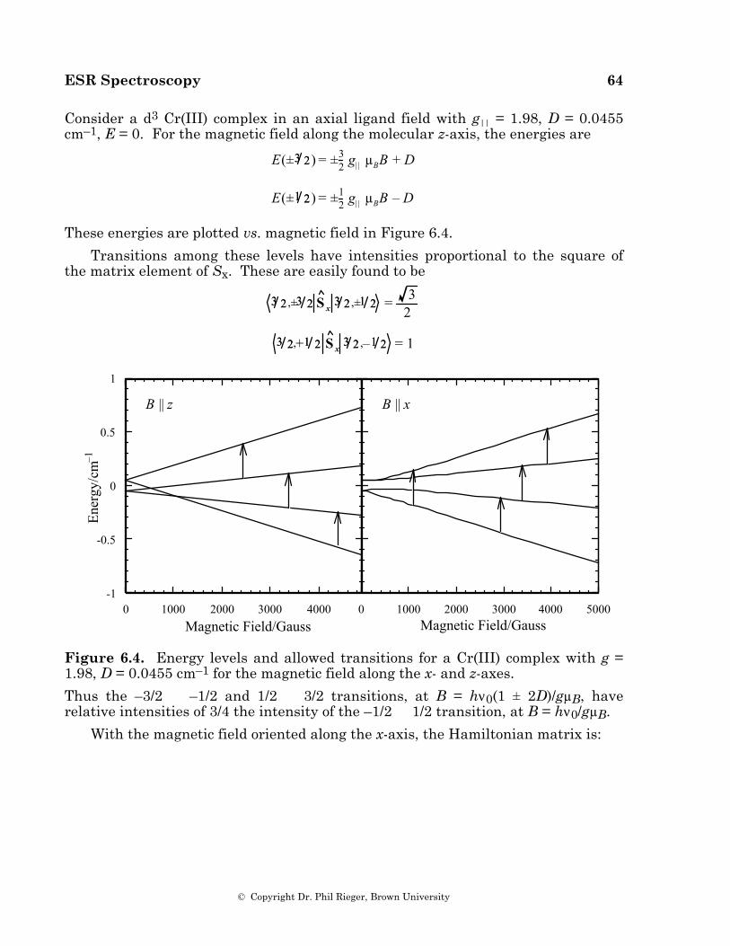
ESR Spectroscopy 64


Consider a d3 Cr(III) complex in an axial ligand field with g|| = 1.98, D = 0.0455 cm–1, E = 0. For the magnetic field along the molecular z-axis, the energies are

E(±3 23 2) = ±3

2 g| | µBB + D

E(±1 21 2) = ±1

2 g| | µBB – D

These energies are plotted vs. magnetic field in Figure 6.4.

Transitions among these levels have intensities proportional to the square of the matrix element of Sx. These are easily found to be

3 23 2,±3 23 2 S x

3 23 2,±1 21 2 = 32

3 23 2,+1 21 2 S x

3 23 2,–1 21 2 = 1

-1

-0.5

0

0.5

1

Ene

rgy/

cm–1


B || z


B || x

Figure 6.4. Energy levels and allowed transitions for a Cr(III) complex with g = 1.98, D = 0.0455 cm–1 for the magnetic field along the x- and z-axes.

Thus the –3/2 ∅ –1/2 and 1/2 ∅ 3/2 transitions, at B = hν0(1 ± 2D)/gµB, have relative intensities of 3/4 the intensity of the –1/2 ∅ 1/2 transition, at B = hν0/gµB.

With the magnetic field oriented along the x-axis, the Hamiltonian matrix is:

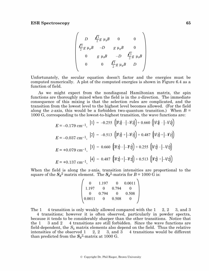
ESR Spectroscopy 65


D 3

2 g⊥µBB 0 0

32 g⊥µBB –D g⊥µBB 0

0 g⊥µBB –D 32 g⊥µBB

0 0 32

g⊥µBB D

Unfortunately, the secular equation doesn't factor and the energies must be computed numerically. A plot of the computed energies is shown in Figure 6.4 as a function of field.

As we might expect from the nondiagonal Hamiltonian matrix, the spin functions are thoroughly mixed when the field is in the x-direction. The immediate consequence of this mixing is that the selection rules are complicated, and the transition from the lowest level to the highest level becomes allowed. (For the field along the z-axis, this would be a forbidden two-quantum transition.) When B = 1000 G, corresponding to the lowest-to-highest transition, the wave functions are:

E = –0.179 cm–1, 1 = –0.255 3 23 2 – –3 23 2 + 0.660 1 21 2 – –1 21 2

E = –0.037 cm–1, 2 = –0.513 3 23 2 + –3 23 2 + 0.487 1 21 2 + –1 21 2

E = +0.079 cm–1, 3 = 0.660 3 23 2 – –3 23 2 + 0.255 1 21 2 – –1 21 2

E = +0.137 cm–1, 4 = 0.487 3 23 2 + –3 23 2 + 0.513 1 21 2 + –1 21 2

When the field is along the x-axis, transition intensities are proportional to the square of the Sz2 matrix element. The Sz2-matrix for B = 1000 G is:

0 1.197 0 0.0011

1.197 0 0.794 00 0.794 0 0.508

0.0011 0 0.508 0

The 1 ∅ 4 transition is only weakly allowed compared with the 1 ∅ 2, 2 ∅ 3, and 3 ∅ 4 transitions; however it is often observed, particularly in powder spectra, because it tends to be considerably sharper than the other transitions. Notice that the 1 ∅ 3 and 2 ∅ 4 transitions are still forbidden. Since the wave functions are field-dependent, the Sz matrix elements also depend on the field. Thus the relative intensities of the observed 1 ∅ 2, 2 ∅ 3, and 3 ∅ 4 transitions would be different than predicted from the Sz2-matrix at 1000 G.

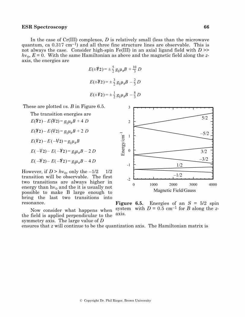
ESR Spectroscopy 66


In the case of Cr(III) complexes, D is relatively small (less than the microwave quantum, ca 0.317 cm–1) and all three fine structure lines are observable. This is not always the case. Consider high-spin Fe(III) in an axial ligand field with D >> hνo, E = 0. With the same Hamiltonian as above and the magnetic field along the z-axis, the energies are

E(±5 25 2) = ± 5

2 g||µBB + 103 D

E(±3 23 2) = ± 3

2 g||µBB – 23 D

E(±1 21 2) = ± 1

2 g||µBB – 83 D

These are plotted vs. B in Figure 6.5.

The transition energies are

E(5 25 2) – E (3 23 2) = g||µBB + 4 D

E(3 23 2) – E (1 21 2) = g||µBB + 2 D

E(1 21 2) – E ( –1 21 2) = g||µBB

E( –1 21 2) – E( –3 23 2) = g||µBB – 2 D

E( –3 23 2) – E( –5 25 2) = g||µBB – 4 D

However, if D > hνo, only the –1/2 ∅ 1/2 transition will be observable. The first two transitions are always higher in energy than hνo and the it is usually not possible to make B large enough to bring the last two transitions into resonance.

Now consider what happens when the field is applied perpendicular to the symmetry axis. The large value of D

-2

-1

0

1

2

3

Ene

rgy/

cm–1


5/2

–5/2

3/2

–3/21/2

–1/2

Figure 6.5. Energies of an S = 5/2 spin system with D = 0.5 cm–1 for B along the z-axis.

ensures that z will continue to be the quantization axis. The Hamiltonian matrix is

ESR Spectroscopy 67


103 D 5 g⊥µBB 0 0 0 0

5 g⊥µBB – 23 D 2 g⊥µBB 0 0 0

0 2 g⊥µBB – 83 D 3

2 g⊥µBB 0 0

0 0 32 g⊥µBB – 8

3 D 2 g⊥µBB 0

0 0 0 2 g⊥µBB – 23 D 5 g⊥µBB

0 0 0 0 5 g⊥µBB 103 D

We ought to solve a 6∞6 secular equation, but we can get a reasonable approximation more easily. Since D is big, the ±5/2 and ±3/2 levels are well separated from the ±1/2 levels before application of the magnetic field. Thus mixing of 3 2 with 1 2 will be much less important than mixing of 1 2 with -1 2 . Thus we can solve just the middle 2∞2 block for the energies of the mS = ±1/2 levels. The expanded block gives:

– 8

3 D – E2

– 32 g⊥µBB

2= 0

so that the energies are

E = – 8

3 D ± 32 g⊥µBB

and the energy difference is

E(1 21 2) – E ( –1 21 2) = 3 g⊥µBB

The apparent g-value for the transition is 3g⊥, geff = 6 if g⊥ = 2.

Thus high-spin d5 Fe(III) in an axial ligand field should show a resonance around g = 2 when B is along the symmetry axis and a resonance near g = 6 when B is perpendicular to the symmetry axis. In solution, where the complex tumbles rapidly and averages the g-values, the resonance is expected to be so broad as to be undetectable.

ESR Spectroscopy 68


References

1. A. Hudson, Electron Spin Resonance, 1988,11A , 55-76.

2. P. B. Ayscough, Electron Spin Resonance in Chemistry, Methuen, London, 1967.

3. P. W. Atkins and M. C. R. Symons, The Structure of Inorganic Radicals, Elsevier, Amsterdam, 1967.

4. A. Abragam and B. Bleaney, Electron Paramagnetic Resonance of Transition Ions, Clarendon Press, Oxford, 1970.

5. J. E. Wertz and J. E. Bolton, Electron Spin Resonance, McGraw-Hill, New York, 1972.

6. N. M. Atherton, Electron Spin Resonance, Ellis Horwood, Chicester, 1973.

7. W. Gordy, Theory and Applications of Electron Spin Resonance, Wiley, New York, 1980.

8. J. R. Pilbrow, Transition Ion Electron Paramagnetic Resonance, Clarendon Press, Oxfor, 1990.

9. F. E. Mabbs and D. Collison, Electron Paramagnetic Resonance of d Transition Metal Compounds, Elsevier, Amsterdam, 1992.

10. G. Breit and I. I. Rabi, Phys. Rev. 1931, 38, 2082-2083.

11. S. I. Weissman, J. Townsend, G. E. Paul, and G. E. Pake, J. Chem. Phys. 1953, 21, 2227.

12. L. V. Casagrande, T. Chen, P. H. Rieger, B. H. Robinson, J. Simpson, and S. J. Visco, Inorg. Chem. 1985, 23, 2019-2025.

13. B. M. Peake, P. H. Rieger, B. H. Robinson, and J. Simpson, Inorg. Chem. 1979,18, 1000-1005.

14. A. R. Boate, J. R. Morton, and K. F. Preston, J. Mag. Reson. 1976, 24, 259-268.

15. R. W. Fessenden and R. H. Schuler, J. Chem. Phys. 1963, 39, 2147.

16. M. Karplus and G. K. Fraenkel, J. Chem. Phys. 1961, 35, 1312.

17. R. Wilson and D. Kivelson, J. Chem. Phys. 1966, 44, 154; P. W. Atkins and D. Kivelson, J. Chem. Phys. 1966, 44, 169.

18. G. K. Fraenkel, J. Phys. Chem. 1967, 71, 139-171.

19. W. B. Lewis and L. O. Morgan, in R. L. Carlin (Ed.), Transition Met. Chem., Vol. 4, Marcel Dekker, New York, 1968, pp. 33-112.

20. B. H. Robinson and A. H. Beth, Electron Spin Resonance 1983,8, 346-377.

21. M. M. Iannuzzi and P. H. Rieger, Inorg. Chem. 1975,14, 2895-2899.

22. M. M. Iannuzzi, C. P. Kubiak, and P. H. Rieger, J. Phys. Chem. 1976,80, 541-545.

ESR Spectroscopy 69


23. R. L. Ward and S. I. Weissman, J. Am. Chem. Soc. 1957,79, 2086-2090.

24. B. J. Corden and P. H. Rieger, Inorg. Chem. 1971,10, 263-272.

25. H. S. Gutowsky, D. W. McCall, and C. P. Slichter, J. Chem. Phys. 1953, 21, 279-292. See also reference 6, pp 309-313.

26. J. I. Kaplan, J. Chem. Phys. 1958, 28, 278-282; 1958, 29, 462; S. Alexander, ibid. 1962, 37, 967-974, 974-980. See also reference 6, pp 313-323.

27. See also reference 6, pp 323-327.

28. N. W. Duffy, R. R. Nelson, M. G. Richmond, A. L. Rieger, P. H. Rieger, B. H. Robinson, D. R. Tyler, J. C. Wang and K. Yang, Inorg. Chem. 1998, 37, 4849.

29. J. A. DeGray, Q. Meng, and P. H. Rieger, J. Chem. Soc. Faraday I 1987, 83, 3565-3573.

30. N. V. Vugman, A. O. Caride, and J. Danon, J. Chem. Phys. 1973, 59, 4418-4422.

31. N. V. Vugman and N. M. Pinhal, Mol. Phys. 1983,49, 1315-1319.

32. J. A. DeGray, P. H. Rieger, N. G. Connelly and G. Garcia, J. Magn. Reson., 1990, 88, 376.

33. P. H. Rieger, J. Magn. Reson. 1982, 50, 485-489.

34. M. C. R. Symons, J. R. Morton, and K. F. Preston, in K. S. Suslick (Ed.), High-Energy Processes in Organometallic Chemistry, American Chemical Society, Washington, DC, 1987, pp. 169-190.

35. P. C. Taylor, J. F. Baugher, and H. M. Kriz, Chem. Rev. 1975, 75, 203-240.

36. I. V. Ovchinnikov and V. N. Konstantinov, J. Magn. Reson. 1978, 32, 179-190.

37. P. C. Taylor and P. J. Bray, J. Magn. Reson. 1970, 2, 305-331.

38. J. A. DeGray and P. H. Rieger, Bull. Magn. Reson. 1987, 8, 95-101.

39. B. A. Goodman and J. B. Raynor, Adv. Inorg. Chem. Radiochem. 1971, 13, 136-362.

40. J. R. Morton and K .F. Preston, J. Mag. Reson. 1978, 30, 577-582.

41. A. K. Koh and D. J. Miller, Atom. Data Nucl. Data Tab. 1985, 33, 235-253.

42. P. H. Rieger, J. Mag. Reson. 1997, 124, 140.

43. B. M. Peake, P. H. Rieger, B. H. Robinson, and J. Simpson, J. Am. Chem. Soc. 1980, 102, 156-163.

44. N. G. Connelly, W. E. Geiger, G. A. Lane, S. J. Raven, and P. H. Rieger, J. Am. Chem. Soc. 1986,108, 6219-6224.

45. B. R. McGarvey, in T. F. Yen (Ed.), Electron Spin Resonance of Metal Complexes, Plenum Press, New York, 1969, pp. 1-11.

ESR Spectroscopy 70


46. A. F. Stone, Proc. Roy. Soc. (London) 1963, A271, 424-434.

47. T. Kawamura, K. Fukamachi, T. Sowa, S. Hayashide, and T. Yonezawa, J. Am. Chem. Soc. 1981, 103, 364-369.

48. G. A. Carriedo, V. Riera, N. G. Connelly, and S. J. Raven, J. Chem. Soc., Dalton Trans.1987, 1769-1773.

49. G. A. Carriedo, N. G. Connelly, E. Perez-Carreno, A. G. Orpen, A. L. Rieger, P. H. Rieger, V. Riera, and G. M. Rosair, J. Chem. Soc., Dalton Trans., 1993, 3103.

50. T. A. Albright, W. E. Geiger, J. Moraczweski, and B. Tulyathan, J. Am. Chem. Soc. 1981, 103, 4787-4794.

51. T. A. Albright and R. Hoffmann, Chem. Ber. 1978, 111, 1578-1590.

52. J. R. Pilbrow and M. R. Lowrey, Rep. Prog. Phys. 1980, 43, 433-495.

53. F. K. Kneubühl, Phys. Kondens. Mat. 1963, 1, 410-447; 1965, 4, 50-62.

54. For a summary of Kneubühl's methods, see reference 52.

55. W. E. Geiger, P. H. Rieger, B. Tulyathan, and M. C. Rausch, J. Am. Chem. Soc. 1984, 106, 7000-7006.

56. T. Lionel, J. R. Morton, and K. F. Preston, J. Chem. Phys. 1982, 76, 234-239.

57. S. A. Fairhurst, J. R. Morton, and K. F. Preston, J. Chem. Phys. 1982, 77, 5872-5875.

58. D. J. Hammack, M. M. Dillard, M. P. Castellani, A. L. Rheingold, A. L. Rieger and P. H. Rieger,Organometallics, 1996, 15, 4791.

59. B. M. Peake, P. H. Rieger, B. H. Robinson, and J. Simpson, J. Am. Chem. Soc. 1980, 102, 156.

60. B. M. Peake, P. H. Rieger, B. H. Robinson, and J. Simpson, Inorg. Chem. 1981, 20, 2540.

61. F. A. Cotton, J. D. Jamerson, and B. R. Stults, J. Am. Chem. Soc. 1976, 98, 1774-1779.

62. C. G. Howard, G. S. Girolami, G. Wilkinson, M. Thornton-Pett, and M. B. Hursthouse, J. Chem. Soc., Dalton Trans. 1983, 2631-2637.

ESR Spectroscopy 71


Problems

1. The tetramethylammonium salt of the 1,1,2,3,3-pentacyanopropenyl anion, [(NC)2C-C(CN)=C(CN)2]–, was reduced electrochemically at room temperature in N,N-dimethylformamide solution containing tetramethylammonium perchlorate as a supporting electrolyte. When the reduction was at the potential of the first polarographic wave, ESR spectrum (a), shown below, was observed. When the potential was changed to that of the second reduction wave, however, spectrum (b) was observed.

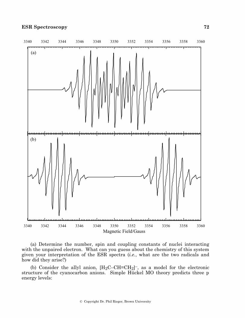
ESR Spectroscopy 72


3340 3342 3344 3346 3348 3350 3352 3354 3356 3358 3360

3340 3342 3344 3346 3348 3350 3352 3354 3356 3358 3360Magnetic Field/Gauss

(a)

(b)

(a) Determine the number, spin and coupling constants of nuclei interacting with the unpaired electron. What can you guess about the chemistry of this system given your interpretation of the ESR spectra (i.e., what are the two radicals and how did they arise?)

(b) Consider the allyl anion, [H2C–CH=CH2]–, as a model for the electronic structure of the cyanocarbon anions. Simple Hückel MO theory predicts three p energy levels:

ESR Spectroscopy 73


E 1 = α + 2 β ψ1 = 1

2ϕ1 + ϕ3 + 2 ϕ2

E 2 = α ψ2 = 1

2ϕ1 – ϕ3

E 3 = α – 2 β ψ3 = 1

2ϕ1 + ϕ3 – 2 ϕ2

Is this simple theoretical prediction consistent with the ESR results? Explain.

2. The PO32– radical, produced by γ-irradiation of Na2HPO3.5H2O crystals, gives an axially symmetric ESR spectrum with g|| = 1.999, g⊥ = 2.001 and a 31P coupling matrix with a|| = 699 G, a⊥ = 540 G. For an electron in a phosphorus 3s orbital, one expects a coupling constant of 3664 G; for an electron in a phosphorus 3p orbital, the dipolar coupling parameter is P = 251.8 G.

(a) The signs of the experimental couplings are indeterminate. What combination of signs makes physical sense?

(b) Compute the phosphorus 3p contribution and the minimum and maximum 3s contribution to the MO containing the odd electron. What is the minimum and maximum spin density on each oxygen?

3. The radical anion [PhCCo3(CO)9]–, obtained by reduction of the neutral cluster in THF solution, gives a 22-line isotropic spectrum (see Figure 4.3) with g = 2.013, A Co = 33.6 ∞ 10-4 cm–1. From analysis of the line shapes, it is clear that the three cobalt nuclei are magnetically equivalent (cobalt is 100% 59Co, I = 7/2). The frozen solution gives a spectrum which shows well-resolved parallel features, g|| = 1.996, A|| = 73.6 ∞ 10–4 cm–1. The perpendicular features of the spectrum are not resolved; the linewidths could hide a perpendicular coupling of as much as 20 ∞ 10–4 cm–1.

(a) The signs of A and A|| are experimentally indeterminate. However, the small magnitude of A⊥ and the relationship, A = (A|| + 2A⊥)/3, imposes some limitations. What signed values for A , A||, and A⊥ are consistent with the experimental data?

(b) Assuming that the molecular symmetry is C3v, use the symmetry restrictions summarized in Table 5 and the accompanying discussion to determine the orientation of the principal axes of the g-matrix. What restrictions are imposed by symmetry on the orientations of the hyperfine matrix principal axes? (Strictly speaking, the phenyl group reduces the symmetry to Cs or less; however, virtually identical spectra are obtained when -Ph is replaced by -CH3 so it seems safe to ignore the substituent.)

(c) The parallel features of the frozen solution spectrum are equally spaced within experimental error. This suggests that the three cobalt nuclear hyperfine matrixs have the corresponding axis in common. What must be the orientation of this common axis?

(d) Consider the following local axes for the three cobalt atoms: let the x-axes be normal to the reflection planes, the z-axes be directed toward the center of the tricobalt plane, and the y-axes be parallel to the three-fold molecular axis. Now

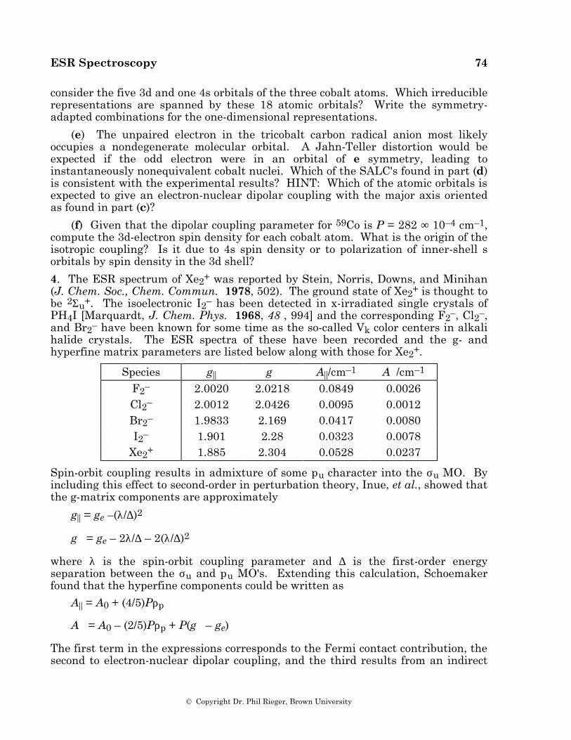
ESR Spectroscopy 74


consider the five 3d and one 4s orbitals of the three cobalt atoms. Which irreducible representations are spanned by these 18 atomic orbitals? Write the symmetry-adapted combinations for the one-dimensional representations.

(e) The unpaired electron in the tricobalt carbon radical anion most likely occupies a nondegenerate molecular orbital. A Jahn-Teller distortion would be expected if the odd electron were in an orbital of e symmetry, leading to instantaneously nonequivalent cobalt nuclei. Which of the SALC's found in part (d) is consistent with the experimental results? HINT: Which of the atomic orbitals is expected to give an electron-nuclear dipolar coupling with the major axis oriented as found in part (c)?

(f) Given that the dipolar coupling parameter for 59Co is P = 282 ∞ 10–4 cm–1, compute the 3d-electron spin density for each cobalt atom. What is the origin of the isotropic coupling? Is it due to 4s spin density or to polarization of inner-shell s orbitals by spin density in the 3d shell?

4. The ESR spectrum of Xe2+ was reported by Stein, Norris, Downs, and Minihan (J. Chem. Soc., Chem. Commun. 1978, 502). The ground state of Xe2+ is thought to be 2Σu+. The isoelectronic I2– has been detected in x-irradiated single crystals of PH4I [Marquardt, J. Chem. Phys. 1968, 48 , 994] and the corresponding F2–, Cl2–, and Br2– have been known for some time as the so-called Vk color centers in alkali halide crystals. The ESR spectra of these have been recorded and the g- and hyperfine matrix parameters are listed below along with those for Xe2+.

Species g|| g⊥ A||/cm–1 A⊥/cm–1 F2– 2.0020 2.0218 0.0849 0.0026 Cl2– 2.0012 2.0426 0.0095 0.0012 Br2– 1.9833 2.169 0.0417 0.0080 I2– 1.901 2.28 0.0323 0.0078

Xe2+ 1.885 2.304 0.0528 0.0237

Spin-orbit coupling results in admixture of some pu character into the σu MO. By including this effect to second-order in perturbation theory, Inue, et al., showed that the g-matrix components are approximately

g|| = ge –(λ/∆)2

g⊥ = ge – 2λ/∆ – 2(λ/∆)2

where λ is the spin-orbit coupling parameter and ∆ is the first-order energy separation between the σu and pu MO's. Extending this calculation, Schoemaker found that the hyperfine components could be written as

A|| = A0 + (4/5)Pρp

A⊥ = A0 – (2/5)Pρp + P(g⊥ – ge)

The first term in the expressions corresponds to the Fermi contact contribution, the second to electron-nuclear dipolar coupling, and the third results from an indirect

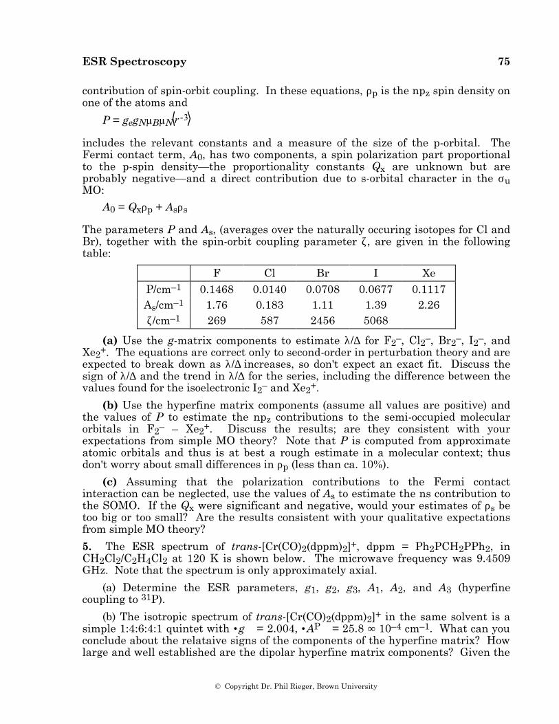
ESR Spectroscopy 75


contribution of spin-orbit coupling. In these equations, ρp is the npz spin density on one of the atoms and

P = gegNµBµN r -3

includes the relevant constants and a measure of the size of the p-orbital. The Fermi contact term, A0, has two components, a spin polarization part proportional to the p-spin density—the proportionality constants Qx are unknown but are probably negative—and a direct contribution due to s-orbital character in the σu MO:

A0 = Qxρp + Asρs

The parameters P and As, (averages over the naturally occuring isotopes for Cl and Br), together with the spin-orbit coupling parameter ζ, are given in the following table:

F Cl Br I Xe P/cm–1 0.1468 0.0140 0.0708 0.0677 0.1117 As/cm–1 1.76 0.183 1.11 1.39 2.26 ζ/cm–1 269 587 2456 5068

(a) Use the g-matrix components to estimate λ/∆ for F2–, Cl2–, Br2–, I2–, and Xe2+. The equations are correct only to second-order in perturbation theory and are expected to break down as λ/∆ increases, so don't expect an exact fit. Discuss the sign of λ/∆ and the trend in λ/∆ for the series, including the difference between the values found for the isoelectronic I2– and Xe2+.

(b) Use the hyperfine matrix components (assume all values are positive) and the values of P to estimate the npz contributions to the semi-occupied molecular orbitals in F2– – Xe2+. Discuss the results; are they consistent with your expectations from simple MO theory? Note that P is computed from approximate atomic orbitals and thus is at best a rough estimate in a molecular context; thus don't worry about small differences in ρp (less than ca. 10%).

(c) Assuming that the polarization contributions to the Fermi contact interaction can be neglected, use the values of As to estimate the ns contribution to the SOMO. If the Qx were significant and negative, would your estimates of ρs be too big or too small? Are the results consistent with your qualitative expectations from simple MO theory?

5. The ESR spectrum of trans-[Cr(CO)2(dppm)2]+, dppm = Ph2PCH2PPh2, in CH2Cl2/C2H4Cl2 at 120 K is shown below. The microwave frequency was 9.4509 GHz. Note that the spectrum is only approximately axial.

(a) Determine the ESR parameters, g1, g2, g3, A1, A2, and A3 (hyperfine coupling to 31P).

(b) The isotropic spectrum of trans-[Cr(CO)2(dppm)2]+ in the same solvent is a simple 1:4:6:4:1 quintet with •g = 2.004, •AP = 25.8 ∞ 10–4 cm–1. What can you conclude about the relataive signs of the components of the hyperfine matrix? How large and well established are the dipolar hyperfine matrix components? Given the

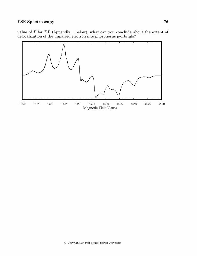
ESR Spectroscopy 76


value of P for 31P (Appendix 1 below), what can you conclude about the extent of delocalization of the unpaired electron into phosphorus p-orbitals?

3250 3275 3300 3325 3350 3375 3400 3425 3450 3475 3500Magnetic Field/Gauss

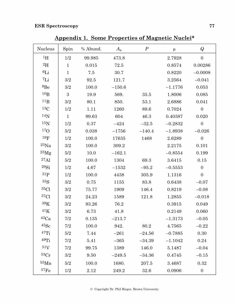
ESR Spectroscopy 77


Appendix 1. Some Properties of Magnetic Nuclei*

Nucleus Spin % Abund. As P µ Q

1H 1/2 99.985 473.8 2.7928 0 2H 1 0.015 72.5 0.8574 0.00286 6Li 1 7.5 30.7 0.8220 –0.0008 7Li 3/2 92.5 121.7 3.2564 –0.041 9Be 3/2 100.0 –150.6 –1.1776 0.053 10B 3 19.9 569. 35.5 1.8006 0.085 11B 3/2 80.1 850. 53.1 2.6886 0.041 13C 1/2 1.11 1260 89.6 0.7024 0 14N 1 99.63 604 46.3 0.40387 0.020 15N 1/2 0.37 –424 –32.5 –0.2832 0 17O 5/2 0.038 –1756 –140.4 –1.8938 –0.026 19F 1/2 100.0 17635 1468 2.6289 0

23Na 3/2 100.0 309.2 2.2175 0.101 25Mg 5/2 10.0 –162.1 –0.8554 0.199 27Al 5/2 100.0 1304 69.3 3.6415 0.15 29Si 1/2 4.67 –1532 –95.2 –0.5553 0 31P 1/2 100.0 4438 305.9 1.1316 0 33S 3/2 0.75 1155 83.8 0.6438 –0.07 35Cl 3/2 75.77 1909 146.4 0.8219 –0.08 37Cl 3/2 24.23 1589 121.8 1.2855 –0.018 39K 3/2 93.26 76.2 0.3915 0.049 41K 3/2 6.73 41.8 0.2149 0.060

43Ca 7/2 0.135 –213.7 –1.3173 –0.05 45Sc 7/2 100.0 942. 80.2 4.7565 –0.22 47Ti 5/2 7.44 –261 –24.56 –0.7885 0.30 49Ti 7/2 5.41 –365 –34.39 –1.1042 0.24 51V 7/2 99.75 1389 146.0 5.1487 –0.04 53Cr 3/2 9.50 –249.5 –34.36 0.4745 –0.15 55Mn 5/2 100.0 1680. 207.5 3.4687 0.32 57Fe 1/2 2.12 249.2 32.6 0.0906 0

ESR Spectroscopy 78


* As and P in units of 10–4 cm–1; µ in units of nm, Q in units of 10–28 m2

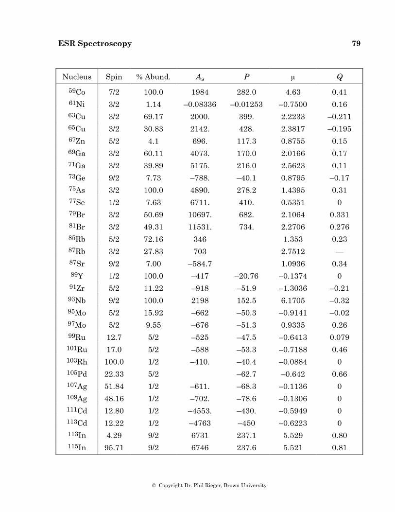
ESR Spectroscopy 79



59Co 7/2 100.0 1984 282.0 4.63 0.41 61Ni 3/2 1.14 –0.08336 –0.01253 –0.7500 0.16 63Cu 3/2 69.17 2000. 399. 2.2233 –0.211 65Cu 3/2 30.83 2142. 428. 2.3817 –0.195 67Zn 5/2 4.1 696. 117.3 0.8755 0.15 69Ga 3/2 60.11 4073. 170.0 2.0166 0.17 71Ga 3/2 39.89 5175. 216.0 2.5623 0.11 73Ge 9/2 7.73 –788. –40.1 0.8795 –0.17 75As 3/2 100.0 4890. 278.2 1.4395 0.31 77Se 1/2 7.63 6711. 410. 0.5351 0 79Br 3/2 50.69 10697. 682. 2.1064 0.331 81Br 3/2 49.31 11531. 734. 2.2706 0.276 85Rb 5/2 72.16 346 1.353 0.23 87Rb 3/2 27.83 703 2.7512 — 87Sr 9/2 7.00 –584.7 1.0936 0.34 89Y 1/2 100.0 –417 –20.76 –0.1374 0 91Zr 5/2 11.22 –918 –51.9 –1.3036 –0.21 93Nb 9/2 100.0 2198 152.5 6.1705 –0.32 95Mo 5/2 15.92 –662 –50.3 –0.9141 –0.02 97Mo 5/2 9.55 –676 –51.3 0.9335 0.26 99Ru 12.7 5/2 –525 –47.5 –0.6413 0.079 101Ru 17.0 5/2 –588 –53.3 –0.7188 0.46 103Rh 100.0 1/2 –410. –40.4 –0.0884 0 105Pd 22.33 5/2 –62.7 –0.642 0.66 107Ag 51.84 1/2 –611. –68.3 –0.1136 0 109Ag 48.16 1/2 –702. –78.6 –0.1306 0 111Cd 12.80 1/2 –4553. –430. –0.5949 0 113Cd 12.22 1/2 –4763 –450 –0.6223 0 113In 4.29 9/2 6731 237.1 5.529 0.80 115In 95.71 9/2 6746 237.6 5.521 0.81

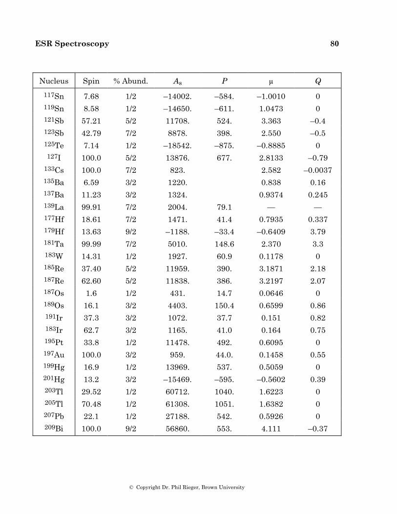
ESR Spectroscopy 80



117Sn 7.68 1/2 –14002. –584. –1.0010 0 119Sn 8.58 1/2 –14650. –611. 1.0473 0 121Sb 57.21 5/2 11708. 524. 3.363 –0.4 123Sb 42.79 7/2 8878. 398. 2.550 –0.5 125Te 7.14 1/2 –18542. –875. –0.8885 0 127I 100.0 5/2 13876. 677. 2.8133 –0.79

133Cs 100.0 7/2 823. 2.582 –0.0037 135Ba 6.59 3/2 1220. 0.838 0.16 137Ba 11.23 3/2 1324. 0.9374 0.245 139La 99.91 7/2 2004. 79.1 — — 177Hf 18.61 7/2 1471. 41.4 0.7935 0.337 179Hf 13.63 9/2 –1188. –33.4 –0.6409 3.79 181Ta 99.99 7/2 5010. 148.6 2.370 3.3 183W 14.31 1/2 1927. 60.9 0.1178 0 185Re 37.40 5/2 11959. 390. 3.1871 2.18 187Re 62.60 5/2 11838. 386. 3.2197 2.07 187Os 1.6 1/2 431. 14.7 0.0646 0 189Os 16.1 3/2 4403. 150.4 0.6599 0.86 191Ir 37.3 3/2 1072. 37.7 0.151 0.82 183Ir 62.7 3/2 1165. 41.0 0.164 0.75 195Pt 33.8 1/2 11478. 492. 0.6095 0 197Au 100.0 3/2 959. 44.0. 0.1458 0.55 199Hg 16.9 1/2 13969. 537. 0.5059 0 201Hg 13.2 3/2 –15469. –595. –0.5602 0.39 203Tl 29.52 1/2 60712. 1040. 1.6223 0 205Tl 70.48 1/2 61308. 1051. 1.6382 0 207Pb 22.1 1/2 27188. 542. 0.5926 0 209Bi 100.0 9/2 56860. 553. 4.111 –0.37

ESR Spectroscopy 81


Appendix 2. The Bloch Equations

The phenomenological equations proposed by Felix Bloch in 1946 have had a profound effect on the development of magnetic resonance, both ESR and NMR, on the ways in which the experiments are described (particularly in NMR), and on the analysis of linewidths and saturation behavior. In this appendix, we will describe the phenomenological model, derive the Bloch equations and solve them for steady-state conditions. We will also show how the Bloch equations can be extended to treat inter- and intramolecular exchange phenomena.

The Phenomenological Model

When a magnetic field is applied to an electron or nuclear spin, the spin quantization axis is defined by the field direction. Spins aligned with the field are only slightly lower in energy than those aligned opposed to the field. If we consider an ensemble of spins, the vector sum of all the spin magnetic moments will be a non-zero net magnetic moment or macroscopic magnetization:

M = µi•i (A2.1)

At equilibrium, M is in the direction of the field B. If somehow M is tilted away from B, there will be a torque which causes M to precess about B with the equation of motion

dMdt

= γB×M (A2.2)

where γ = 2πgµB/h (or 2πgNµN/h). In addition to the precessional motion, there are two relaxation effects.

If M0 is the equilibrium magnetization along B and Mz is the z-component under nonequilibrium conditions, then we assume that Mz approaches M0 with first-order kinetics:

dMz

dt=

M0 – M z

T 1 (A2.3)

where T1 is the characteristic time for approach to equilibrium (the reciprocal of the rate constant). Since this process involves transfer of energy from the spin system to the surroundings (conventionally called the "lattice"), T1 is called the spin-lattice relaxation time. Since electrons are much more closely coupled to molecular interactions than are nuclei (which are buried in a sea of inner-shell electrons), it is not surprising that T1 for electrons is usually much shorter (on the order of microseconds) than are nuclear T1's (on the order of seconds).

There is a second kind of relaxation process which is at least as important for magnetic resonance as the T1 process. Suppose that M is somehow tilted down

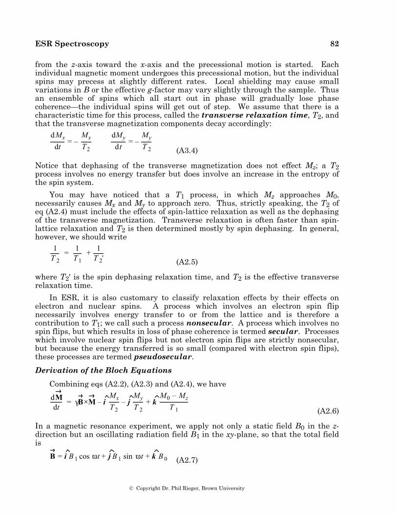
ESR Spectroscopy 82


from the z-axis toward the x-axis and the precessional motion is started. Each individual magnetic moment undergoes this precessional motion, but the individual spins may precess at slightly different rates. Local shielding may cause small variations in B or the effective g-factor may vary slightly through the sample. Thus an ensemble of spins which all start out in phase will gradually lose phase coherence—the individual spins will get out of step. We assume that there is a characteristic time for this process, called the transverse relaxation time, T2, and that the transverse magnetization components decay accordingly:

dMx

dt= –

Mx

T2

dMy

dt= –

My

T 2 (A3.4)

Notice that dephasing of the transverse magnetization does not effect Mz; a T2 process involves no energy transfer but does involve an increase in the entropy of the spin system.

You may have noticed that a T1 process, in which Mz approaches M0, necessarily causes Mx and My to approach zero. Thus, strictly speaking, the T2 of eq (A2.4) must include the effects of spin-lattice relaxation as well as the dephasing of the transverse magnetization. Transverse relaxation is often faster than spin-lattice relaxation and T2 is then determined mostly by spin dephasing. In general, however, we should write

1T 2

= 1T 1

+ 1T 2′ (A2.5)

where T2' is the spin dephasing relaxation time, and T2 is the effective transverse relaxation time.

In ESR, it is also customary to classify relaxation effects by their effects on electron and nuclear spins. A process which involves an electron spin flip necessarily involves energy transfer to or from the lattice and is therefore a contribution to T1; we call such a process nonsecular. A process which involves no spin flips, but which results in loss of phase coherence is termed secular. Processes which involve nuclear spin flips but not electron spin flips are strictly nonsecular, but because the energy transferred is so small (compared with electron spin flips), these processes are termed pseudosecular.

Derivation of the Bloch Equations

Combining eqs (A2.2), (A2.3) and (A2.4), we have

dMdt

= γB×M – iMx

T 2– j

My

T 2+ k

M0 – Mz

T 1 (A2.6)

In a magnetic resonance experiment, we apply not only a static field B0 in the z-direction but an oscillating radiation field B1 in the xy-plane, so that the total field is

B = i B 1 cos ωt + j B 1 sin ωt + k B 0 (A2.7)

ESR Spectroscopy 83


The vector product of eq (A2.6) then becomes:

B×M = –i B 0My – B 1Mz sin ωt + j B 0Mx – B 1Mz cos ωt

+ k B1 M y cos ωt – M x sin ωt

Inserting this expression in eq (A2.6) and separating it into components, we get

dMx

dt= –γB 0My + γB 1Mz sin ωt –

M x

T 2 (A2.8a)

dMy

dt= γB 0Mx – γB 1Mz cos ωt –

My

T 2 (A2.8b)

dMz

dt= γB 1 My cos ωt – Mx sin ωt +

M0 – Mz

T 1 (A2.8c)

It is convenient to write Mx and My as

Mx = u cos ωt + v sin ωt (A2.9a)

My = u sin ωt – v cos ωt (A2.9b)

or u = Mx cos ωt + My sin ωt (A2.10a)

v = Mx sin ωt – My cos ωt (A2.10b)

This is equivalent to transformation to a coordinate system which rotates with the oscillating field; u is that part of Mx which is in-phase with B1 and v is the part which is 90° out of phase. Differentiating eq (A2.10a) and substituting eqs (A2.8a) and (A2.8b), we get

dudt

=dM x

dtcos ωt – M xω sin ωt +

dMy

dtsin ωt + Myω cos ωt

dudt

= γB 0 – ω Mx sin ωt – M y cos ωt –Mx cos ωt + My sin ωt

T 2

dudt

= – ω – γB 0 v – uT 2 (A2.11a)

Similarly, we obtain

dvdt

= ω – γB 0 u – vT 2

+ γB 1Mz (A2.11b)

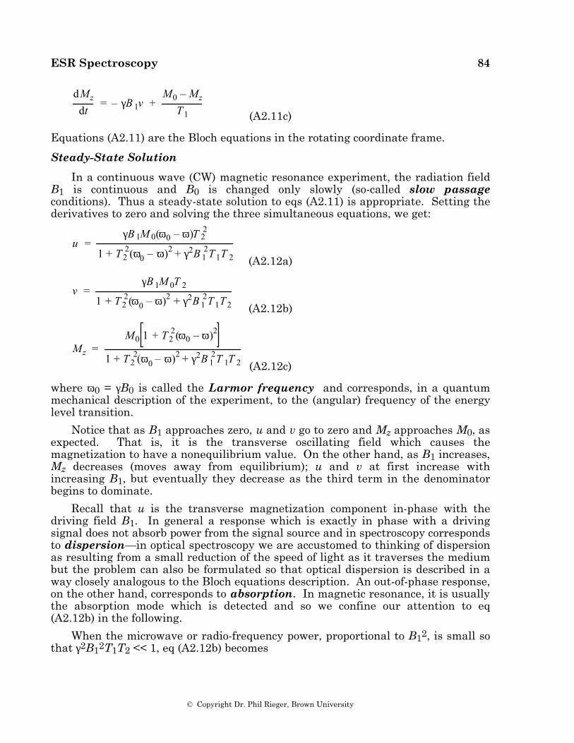
ESR Spectroscopy 84


dMz

dt= – γB 1v +

M0 – Mz

T 1 (A2.11c)

Equations (A2.11) are the Bloch equations in the rotating coordinate frame.

Steady-State Solution

In a continuous wave (CW) magnetic resonance experiment, the radiation field B1 is continuous and B0 is changed only slowly (so-called slow passage conditions). Thus a steady-state solution to eqs (A2.11) is appropriate. Setting the derivatives to zero and solving the three simultaneous equations, we get:

u =

γB 1M 0(ω0 – ω)T 22

1 + T22(ω0 – ω)2 + γ2B 1

2T 1T 2 (A2.12a)

v =

γB 1M 0T 2

1 + T 22(ω0 – ω)2 + γ2B 1

2T 1T 2 (A2.12b)

Mz =M0 1 + T2

2(ω0 – ω)2

1 + T 22(ω0 – ω)2 + γ2B 1

2T 1T 2 (A2.12c)

where ω0 = γB0 is called the Larmor frequency and corresponds, in a quantum mechanical description of the experiment, to the (angular) frequency of the energy level transition.

Notice that as B1 approaches zero, u and v go to zero and Mz approaches M0, as expected. That is, it is the transverse oscillating field which causes the magnetization to have a nonequilibrium value. On the other hand, as B1 increases, Mz decreases (moves away from equilibrium); u and v at first increase with increasing B1, but eventually they decrease as the third term in the denominator begins to dominate.

Recall that u is the transverse magnetization component in-phase with the driving field B1. In general a response which is exactly in phase with a driving signal does not absorb power from the signal source and in spectroscopy corresponds to dispersion—in optical spectroscopy we are accustomed to thinking of dispersion as resulting from a small reduction of the speed of light as it traverses the medium but the problem can also be formulated so that optical dispersion is described in a way closely analogous to the Bloch equations description. An out-of-phase response, on the other hand, corresponds to absorption. In magnetic resonance, it is usually the absorption mode which is detected and so we confine our attention to eq (A2.12b) in the following.

When the microwave or radio-frequency power, proportional to B12, is small so that γ2B12T1T2 << 1, eq (A2.12b) becomes

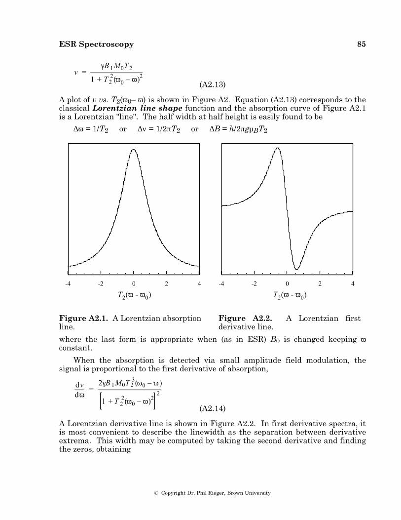
ESR Spectroscopy 85


v =

γB 1M0T 2

1 + T 22(ω0 – ω)2

(A2.13)

A plot of v vs. T2(ω0– ω) is shown in Figure A2. Equation (A2.13) corresponds to the classical Lorentzian line shape function and the absorption curve of Figure A2.1 is a Lorentzian "line". The half width at half height is easily found to be

∆ω = 1/T2 or ∆ν = 1/2πT2 or ∆B = h/2πgµBT2

-4 -2 0 2 4

T2(ω - ω0)

Figure A2.1. A Lorentzian absorption line.

-4 -2 0 2 4

T2(ω - ω0)

Figure A2.2. A Lorentzian first derivative line.

where the last form is appropriate when (as in ESR) B0 is changed keeping ω constant.

When the absorption is detected via small amplitude field modulation, the signal is proportional to the first derivative of absorption,

dvdω

=2γB 1M0T 2

3(ω0 – ω)

1 + T 22(ω0 – ω)2

2

(A2.14)

A Lorentzian derivative line is shown in Figure A2.2. In first derivative spectra, it is most convenient to describe the linewidth as the separation between derivative extrema. This width may be computed by taking the second derivative and finding the zeros, obtaining

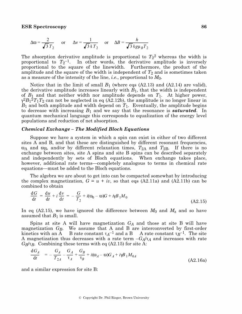
ESR Spectroscopy 86


∆ω = 23 T 2

or ∆ν = 13 š T 2

or ∆B = h3 šgµBT 2

The absorption derivative amplitude is proportional to T22 whereas the width is proportional to T2–1. In other words, the derivative amplitude is inversely proportional to the square of the linewidth. Furthermore, the product of the amplitude and the square of the width is independent of T2 and is sometimes taken as a measure of the intensity of the line, i.e., proportional to M0.

Notice that in the limit of small B1 (where eqs (A2.13) and (A2.14) are valid), the derivative amplitude increases linearly with B1, that the width is independent of B1 and that neither width nor amplitude depends on T1. At higher power, γ2B12T1T2 can not be neglected in eq (A2.12b), the amplitude is no longer linear in B1 and both amplitude and width depend on T1. Eventually, the amplitude begins to decrease with increasing B1 and we say that the resonance is saturated. In quantum mechanical language this corresponds to equalization of the energy level populations and reduction of net absorption.

Chemical Exchange – The Modified Bloch Equations

Suppose we have a system in which a spin can exist in either of two different sites A and B, and that these are distinguished by different resonant frequencies, ωA and ωB, and/or by different relaxation times, T2A and T2B. If there is no exchange between sites, site A spins and site B spins can be described separately and independently by sets of Bloch equations. When exchange takes place, however, additional rate terms—completely analogous to terms in chemical rate equations—must be added to the Bloch equations.

The algebra we are about to get into can be compacted somewhat by introducing the complex magnetization, G = u + iv, so that eqs (A2.11a) and (A2.11b) can be combined to obtain

dGdt

= dudt

+ i dvdt

= – GT 2

+ i(ω0 – ω)G + iγB 1M 0 (A2.15)

In eq (A2.15), we have ignored the difference between M0 and Mz and so have assumed that B1 is small.

Spins at site A will have magnetization GA and those at site B will have magnetization GB. We assume that A and B are interconverted by first-order kinetics with an A ∅ B rate constant τA–1 and a B ∅ A rate constant τB–1. The site A magnetization thus decreases with a rate term –GA/τA and increases with rate GB/τB. Combining these terms with eq (A2.15) for site A:

dGA

dt= –

GA

T 2A–

GA

τA+

GB

τB+ i(ωA – ω)G A + iγB 1M0A

(A2.16a)

and a similar expression for site B:

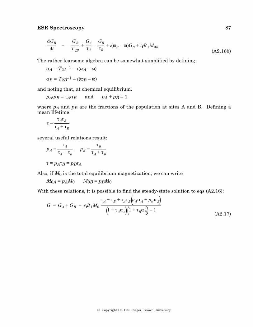
ESR Spectroscopy 87


dGB

dt= –

GB

T 2B+

GA

τA–

GB

τB+ i(ωB – ω)GB + iγB 1M0B

(A2.16b)

The rather fearsome algebra can be somewhat simplified by defining

αA = T2A–1 – i(ωA – ω)

αB = T2B–1 – i(ωB – ω)

and noting that, at chemical equilibrium,

pA/pB = τA/τB and pA + pB = 1

where pA and pB are the fractions of the population at sites A and B. Defining a mean lifetime

τ =

τAτB

τA + τB

several useful relations result:

pA =

τA

τA + τBpB =

τB

τA + τB

τ = pAτB = pBτA

Also, if M0 is the total equilibrium magnetization, we can write M0A = pAM0 M0B = pBM0

With these relations, it is possible to find the steady-state solution to eqs (A2.16):

G = G A + GB = iγB 1M0

τA + τB + τAτB pAαA + pB αB

1 + τAαA 1 + τBαB – 1 (A2.17)

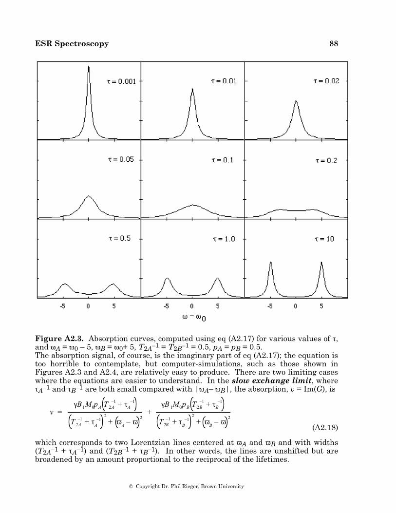
ESR Spectroscopy 88


Figure A2.3. Absorption curves, computed using eq (A2.17) for various values of τ, and ωA = ω0 – 5, ωB = ω0+ 5, T2A–1 = T2B–1 = 0.5, pA = pB = 0.5. The absorption signal, of course, is the imaginary part of eq (A2.17); the equation is too horrible to contemplate, but computer-simulations, such as those shown in Figures A2.3 and A2.4, are relatively easy to produce. There are two limiting cases where the equations are easier to understand. In the slow exchange limit, where τA–1 and τB–1 are both small compared with |ωA– ωB|, the absorption, v = Im(G), is

v =

γB1M0pA T 2A–1 + τA

–1

T 2A–1 + τA

–12

+ ωA – ω2

+γB 1M0pB T 2B

–1 + τB–1

T 2B–1 + τB

–12

+ ωB – ω2

(A2.18)

which corresponds to two Lorentzian lines centered at ωA and ωB and with widths (T2A–1 + τA–1) and (T2B–1 + τB–1). In other words, the lines are unshifted but are broadened by an amount proportional to the reciprocal of the lifetimes.

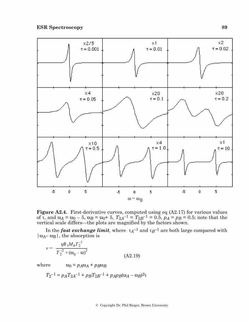
ESR Spectroscopy 89


Figure A2.4. First-derivative curves, computed using eq (A2.17) for various values of τ, and ωA = ω0 – 5, ωB = ω0+ 5, T2A–1 = T2B–1 = 0.5, pA = pB = 0.5; note that the vertical scale differs—the plots are magnified by the factors shown.

In the fast exchange limit, where τA–1 and τB–1 are both large compared with |ωA– ωB|, the absorption is

v =

γB 1M 0T 2-1

T 2-2 + (ω0 – ω)2

(A2.19)

where ω0 = pAωA + pBωB

T2–1 = pAT2A–1 + pBT2B–1 + pApB(ωA – ωB)2τ

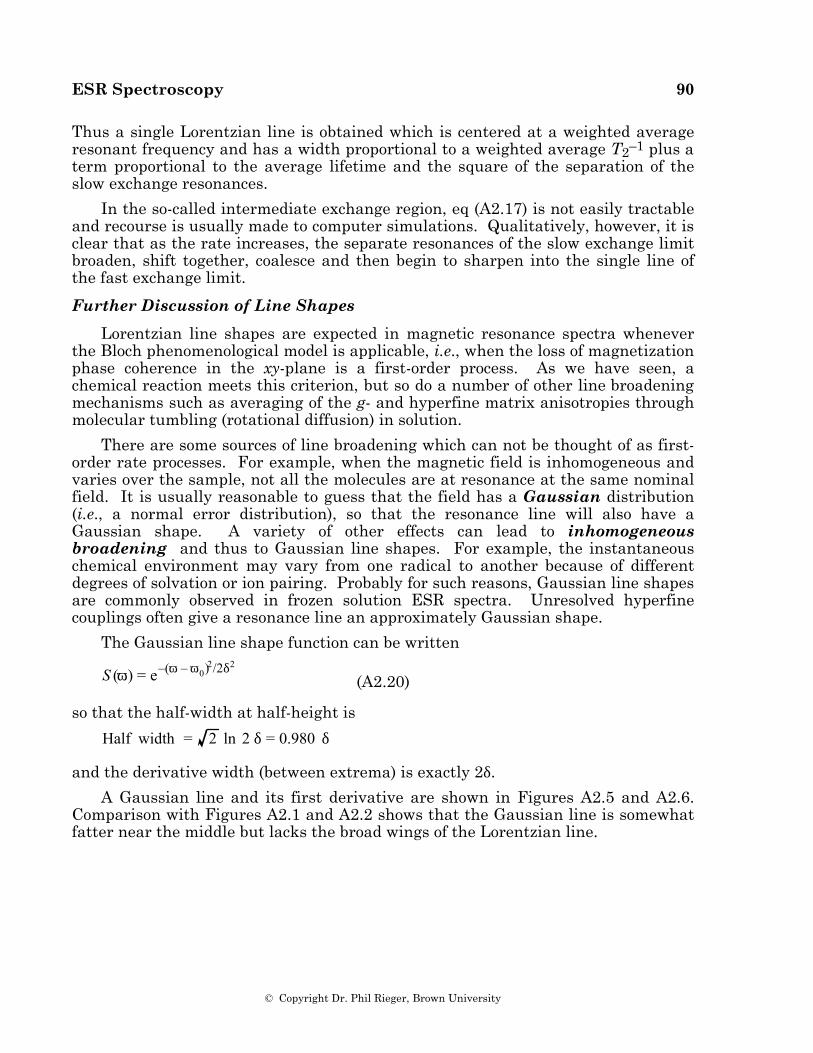
ESR Spectroscopy 90


Thus a single Lorentzian line is obtained which is centered at a weighted average resonant frequency and has a width proportional to a weighted average T2–1 plus a term proportional to the average lifetime and the square of the separation of the slow exchange resonances.

In the so-called intermediate exchange region, eq (A2.17) is not easily tractable and recourse is usually made to computer simulations. Qualitatively, however, it is clear that as the rate increases, the separate resonances of the slow exchange limit broaden, shift together, coalesce and then begin to sharpen into the single line of the fast exchange limit.

Further Discussion of Line Shapes

Lorentzian line shapes are expected in magnetic resonance spectra whenever the Bloch phenomenological model is applicable, i.e., when the loss of magnetization phase coherence in the xy-plane is a first-order process. As we have seen, a chemical reaction meets this criterion, but so do a number of other line broadening mechanisms such as averaging of the g- and hyperfine matrix anisotropies through molecular tumbling (rotational diffusion) in solution.

There are some sources of line broadening which can not be thought of as first-order rate processes. For example, when the magnetic field is inhomogeneous and varies over the sample, not all the molecules are at resonance at the same nominal field. It is usually reasonable to guess that the field has a Gaussian distribution (i.e., a normal error distribution), so that the resonance line will also have a Gaussian shape. A variety of other effects can lead to inhomogeneous broadening and thus to Gaussian line shapes. For example, the instantaneous chemical environment may vary from one radical to another because of different degrees of solvation or ion pairing. Probably for such reasons, Gaussian line shapes are commonly observed in frozen solution ESR spectra. Unresolved hyperfine couplings often give a resonance line an approximately Gaussian shape.

The Gaussian line shape function can be written

S (ω) = e–(ω – ω0)2/2δ2

(A2.20)

so that the half-width at half-height is

Half width = 2 ln 2 δ = 0.980 δ

and the derivative width (between extrema) is exactly 2δ.

A Gaussian line and its first derivative are shown in Figures A2.5 and A2.6. Comparison with Figures A2.1 and A2.2 shows that the Gaussian line is somewhat fatter near the middle but lacks the broad wings of the Lorentzian line.

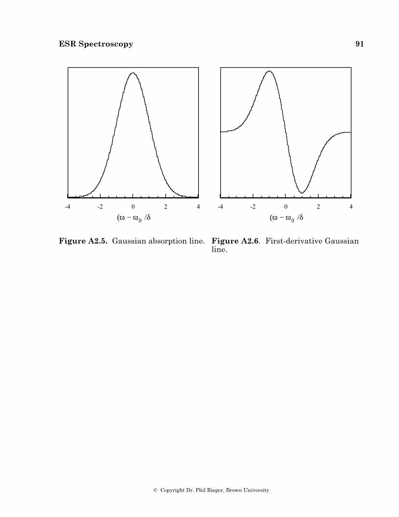
ESR Spectroscopy 91


-4 -2 0 2 4

(ω − ω0)/δ

Figure A2.5. Gaussian absorption line.

-4 -2 0 2 4

(ω − ω0)/δ

Figure A2.6. First-derivative Gaussian line.

ESR Spectroscopy 92


Appendix 4

Interpretation of Isotropic ESR Spectra

The interpretation of an isotropic ESR spectrum is relatively straightforward if a systematic approach is used, but it can be a frustrating experience for a beginner. In these notes, an attempt has been made to give a series of steps which, if followed with care, will result in a succesful interpretation for most reasonably well resolved spectra.

Preliminary Examination of the Spectrum

A. Check to see if the spectrum is symmetric in line positions and relative intensities. If it isn't, then most likely there are two or more radical species. Variation of linewidths with mi may cause the spectrum to appear unsymmetric, but in such a case line positions would still be at least approximately symmetrically distributed about the center.

B. Is there a central line? If there is no central line, then there must be an even number of lines which suggests an odd number of half integral nuclei (i.e., I = 1/2, 3/2, etc.).

C. Are the outermost lines visible above the noise? Observation of the wing lines is often crucial to successful interpretation of ESR spectra. In noisy spectra, it is sometimes difficult to tell if all the lines are actually observed in the wings.

D. How many lines are there? Count them carefully, watching for evidence of unresolved features (shoulders or bumps).

E. What is the ratio of the amplitudes of the biggest to smallest lines in the spectrum?

What do you Expect to See?

A. If the radical was produced by a chemically straightforward procedure, you usually have some idea of the identity of the radical. How many and what kinds of paramagentic nuclei are present?

ESR Spectroscopy 93


B. How many lines are expected from this model? The total number of nuclear spin states is (2I1+1)∞(2I2+1)∞(2I3+1)... Thus if the model structure has six protons (I = 1/2), there should be (2∞1/2 + 1)6 = 26 = 64 nuclear spin states. If some of the nuclei are expected to be equivalent, then the number of lines will be less than the number of spin states, i.e., some of the spin states will be degenerate (to first-order in perturbation theory). Thus if the six protons are in three groups of two, it is as if you had three spin 1 nuclei and you expect (2∞1 + 1)3 = 33 = 27 lines. If there is one group of four equivalent protons and another group of two, then it is as if you had one spin 2 nucleus and one spin 1 nucleus and you expect (2∞2 + 1)(2∞1 + 1) = 15 lines.

C. What is the expected ratio of intensities of the biggest to smallest line? If all the nuclei are inequivalent, then all lines should have the same intensity (barring accidental superpositions). If there are equivalent sets of nuclei, then the expected ratio is the product of the biggest-to-smallest ratios of the various multiplets. Thus for the above examples, three groups of two spin 1/2 nuclei gives a 1:2:1 triplet of 1:2:1 triplets of 1:2:1 triplets; thus the maximum intensity ratio of 2∞2∞2 = 8. If we have a 1:4:6:4:1 quintet of 1:2:1 triplets, then the maximum intensity ratio will be 6∞2 = 12.

Are the Gross Features Consistent with the Model?

A. Compare the number of observed lines with the number expected. If there are more lines than expected, either the model is wrong or there is more than one radical. If the expected and observed numbers are equal, you are in luck—the analysis should be easy. If you see fewer lines than expected (the most common case!), there may be accidental superpositions, small amplitude lines buried under big ones, or just poor resolution. The bigger the discrepancy between expected and observed numbers of lines, the harder the analysis will be.

B. Compare the expected and observed biggest-to-smallest intensity ratios. Accidental degeneracies (or a mI2 linewidth dependence) may cause the observed ratio to be bigger than expected. It is rarer (but not unknown) to find a smaller ratio than expected.

C. Is the presence or absence of a central line consistent with the odd or even number of expected lines?

D. If the model still seems plausible after these tests, go on to a detailed analysis. If there are gross inconsistences, the model is probably wrong.

ESR Spectroscopy 94


Detailed Analysis

A. Measure the positions and amplitudes of all the lines in the spectrum and list them in order in a table. If convenient, measure the line positions in gauss; if this is inconvenient, use arbitrary units such as inches, centimeters, or recorder chart boxes measured from an arbitrary zero. In your table, provide headings for each of the quantum numbers (m1, m2, etc.), for each of the coupling constants (a1, a2, etc.), and for the theoretical intensity (degeneracy).

B. The highest and lowest field lines will always have theoretical intensities of 1 and will have minimum or maximum values for all the quantum numbers. It doesn't really matter whether you start with maximum quantum numbers at the high-field or low-field end of the spectrum—the signs of the coupling constants are indeterminant—but for consistency, let's agree to assign maximum quantum numbers to the lowest field line (i.e., pretend that the coupling constants are positive). Enter these assignments in the table. From this point on, you can work from either end of the spectrum or even from both at once. In the following, we assume that we're working from the low-field end.

C. The spacing between the first and second lines will be the smallest coupling constant, a1. The intensity ratio of these two lines will usually indicate the multiplet to which the coupling constant corresponds. Assign quantum numbers to the second line, compute a1 and enter these numbers in the table. If you have started into a muliplet, you can then predict the positions and intensities of the remaining lines of the muliplet. Find them and enter the quantum numbers and new estimates of a1 in the table.

D. After finding all the lines of the first a1 multiplet, find the first unassigned line. This must correspond to the next larger coupling constant a2. From the ratio of its amplitude to that of the end line, you can usually figure out which multiplet this coupling constant corresponds to. Assign the quantum numbers and compute the coupling constant a2. Enter in the table. This line will also correspond to the first line in a second a1 multiplet, and, knowing a1, you can predict the positions and intensities of the remaining lines of this multiplet. Find them and enter the quantum number assignments and new estimates of a1 and a2 in the table.

E. If a2 corresponds to a multiplet, the positions of the remaining lines can predicted and located. Continue in this way through the spectrum. Small discrepances may arise through measurement errors or because of overlapped lines. A position discrepancy larger than your estimated measurement accuracy, however, may signal a misassignment or inconsistency with the model. Notice that the spacing between the lowest and highest field lines is equal to the sum of the

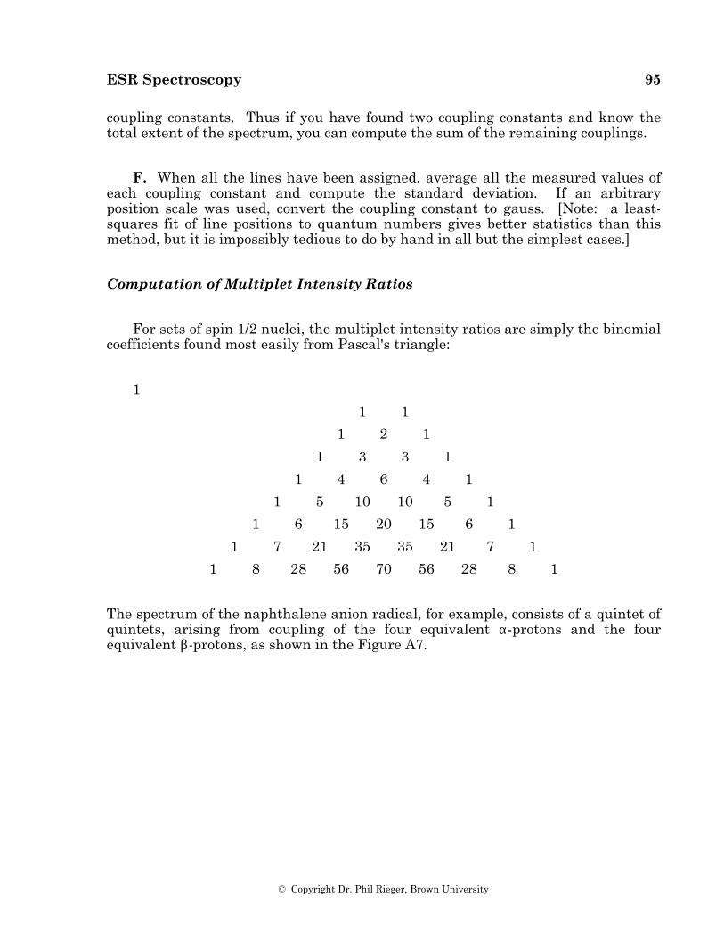
ESR Spectroscopy 95


coupling constants. Thus if you have found two coupling constants and know the total extent of the spectrum, you can compute the sum of the remaining couplings.

F. When all the lines have been assigned, average all the measured values of each coupling constant and compute the standard deviation. If an arbitrary position scale was used, convert the coupling constant to gauss. [Note: a least-squares fit of line positions to quantum numbers gives better statistics than this method, but it is impossibly tedious to do by hand in all but the simplest cases.]

Computation of Multiplet Intensity Ratios

For sets of spin 1/2 nuclei, the multiplet intensity ratios are simply the binomial coefficients found most easily from Pascal's triangle:

1

1 1

1 2 1

1 3 3 1

1 4 6 4 1

1 5 10 10 5 1

1 6 15 20 15 6 1

1 7 21 35 35 21 7 1

1 8 28 56 70 56 28 8 1

The spectrum of the naphthalene anion radical, for example, consists of a quintet of quintets, arising from coupling of the four equivalent α-protons and the four equivalent β-protons, as shown in the Figure A7.

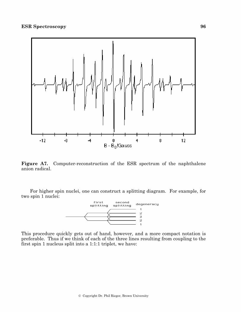
ESR Spectroscopy 96


Figure A7. Computer-reconstruction of the ESR spectrum of the naphthalene anion radical.

For higher spin nuclei, one can construct a splitting diagram. For example, for two spin 1 nuclei:

This procedure quickly gets out of hand, however, and a more compact notation is preferable. Thus if we think of each of the three lines resulting from coupling to the first spin 1 nucleus split into a 1:1:1 triplet, we have:

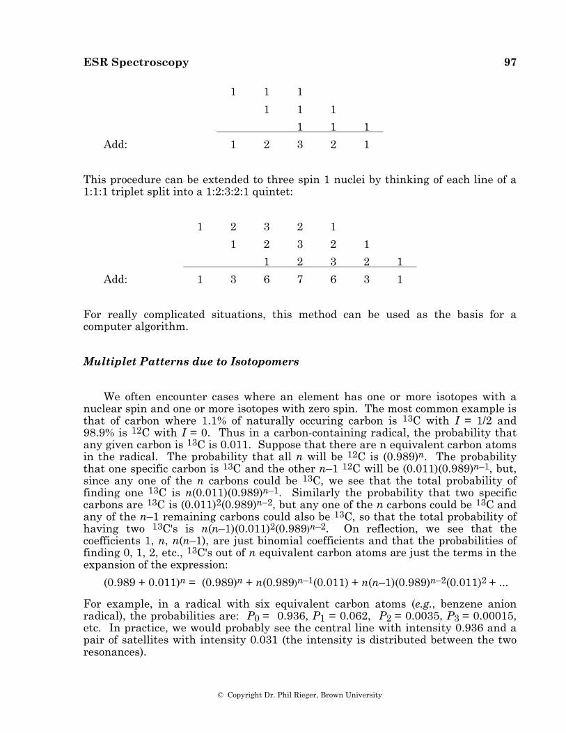
ESR Spectroscopy 97


1 1 1

1 1 1

1 1 1

Add: 1 2 3 2 1

This procedure can be extended to three spin 1 nuclei by thinking of each line of a 1:1:1 triplet split into a 1:2:3:2:1 quintet:

1 2 3 2 1

1 2 3 2 1

1 2 3 2 1

Add: 1 3 6 7 6 3 1

For really complicated situations, this method can be used as the basis for a computer algorithm.

Multiplet Patterns due to Isotopomers

We often encounter cases where an element has one or more isotopes with a nuclear spin and one or more isotopes with zero spin. The most common example is that of carbon where 1.1% of naturally occuring carbon is 13C with I = 1/2 and 98.9% is 12C with I = 0. Thus in a carbon-containing radical, the probability that any given carbon is 13C is 0.011. Suppose that there are n equivalent carbon atoms in the radical. The probability that all n will be 12C is (0.989)n. The probability that one specific carbon is 13C and the other n–1 12C will be (0.011)(0.989)n–1, but, since any one of the n carbons could be 13C, we see that the total probability of finding one 13C is n(0.011)(0.989)n–1. Similarly the probability that two specific carbons are 13C is (0.011)2(0.989)n–2, but any one of the n carbons could be 13C and any of the n–1 remaining carbons could also be 13C, so that the total probability of having two 13C's is n(n–1)(0.011)2(0.989)n–2. On reflection, we see that the coefficients 1, n, n(n–1), are just binomial coefficients and that the probabilities of finding 0, 1, 2, etc., 13C's out of n equivalent carbon atoms are just the terms in the expansion of the expression:

(0.989 + 0.011)n = (0.989)n + n(0.989)n–1(0.011) + n(n–1)(0.989)n–2(0.011)2 + ...

For example, in a radical with six equivalent carbon atoms (e.g., benzene anion radical), the probabilities are: P0 = 0.936, P1 = 0.062, P2 = 0.0035, P3 = 0.00015, etc. In practice, we would probably see the central line with intensity 0.936 and a pair of satellites with intensity 0.031 (the intensity is distributed between the two resonances).

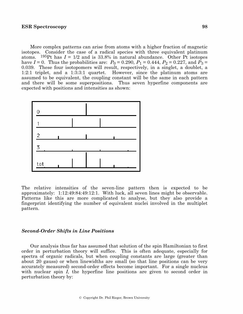
ESR Spectroscopy 98


More complex patterns can arise from atoms with a higher fraction of magnetic isotopes. Consider the case of a radical species with three equivalent platinum atoms. 195Pt has I = 1/2 and is 33.8% in natural abundance. Other Pt isotopes have I = 0. Thus the probabilities are: P0 = 0.290, P1 = 0.444, P2 = 0.227, and P3 = 0.039. These four isotopomers will result, respectively, in a singlet, a doublet, a 1:2:1 triplet, and a 1:3:3:1 quartet. However, since the platinum atoms are assumed to be equivalent, the coupling constant will be the same in each pattern and there will be some superpositions. Thus seven hyperfine components are expected with positions and intensities as shown:

The relative intensities of the seven-line pattern then is expected to be approximately: 1:12:49:84:49:12:1. With luck, all seven lines might be observable. Patterns like this are more complicated to analyse, but they also provide a fingerprint identifying the number of equivalent nuclei involved in the multiplet pattern.

Second-Order Shifts in Line Positions

Our analysis thus far has assumed that solution of the spin Hamiltonian to first order in perturbation theory will suffice. This is often adequate, especially for spectra of organic radicals, but when coupling constants are large (greater than about 20 gauss) or when linewidths are small (so that line positions can be very accurately measured) second-order effects become important. For a single nucleus with nuclear spin I, the hyperfine line positions are given to second order in perturbation theory by:

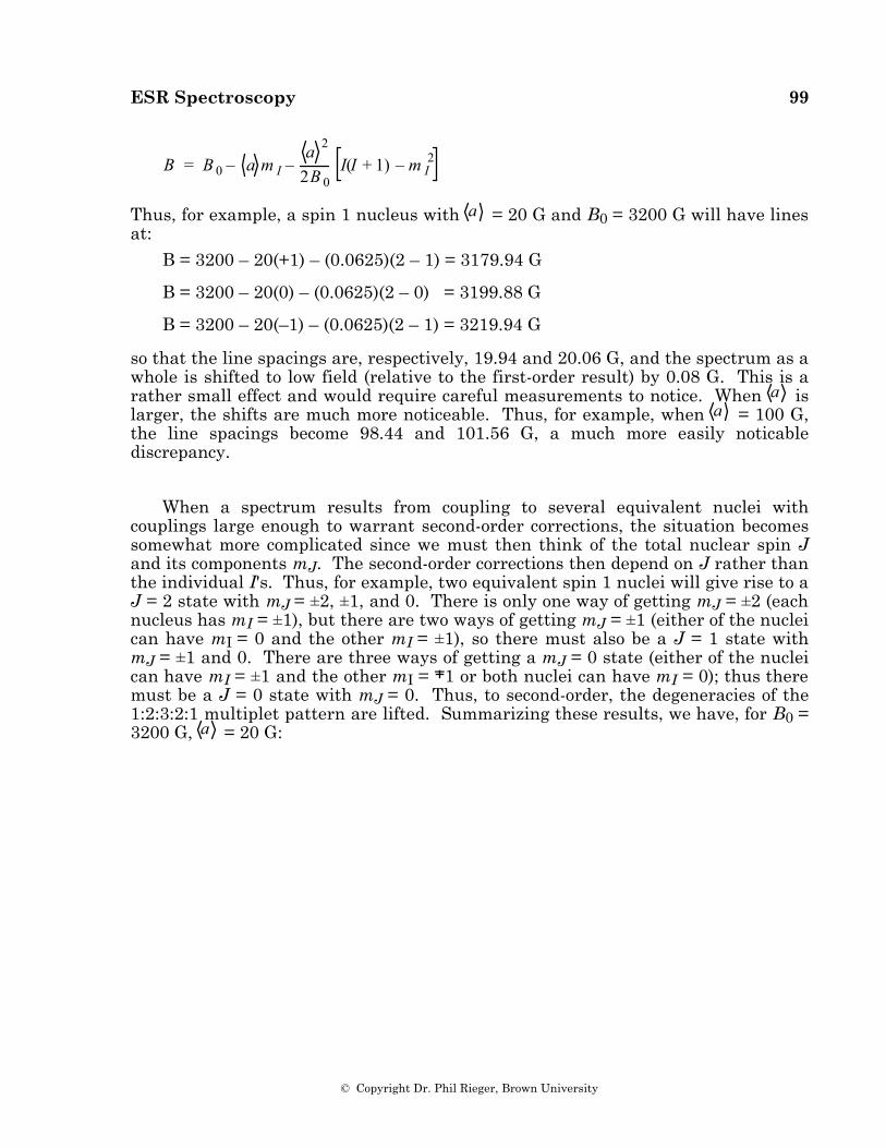
ESR Spectroscopy 99


B = B 0 – a m I –

a 2

2B 0I(I + 1) – m I

2

Thus, for example, a spin 1 nucleus with a = 20 G and B0 = 3200 G will have lines at: B = 3200 – 20(+1) – (0.0625)(2 – 1) = 3179.94 G

B = 3200 – 20(0) – (0.0625)(2 – 0) = 3199.88 G

B = 3200 – 20(–1) – (0.0625)(2 – 1) = 3219.94 G

so that the line spacings are, respectively, 19.94 and 20.06 G, and the spectrum as a whole is shifted to low field (relative to the first-order result) by 0.08 G. This is a rather small effect and would require careful measurements to notice. When a is larger, the shifts are much more noticeable. Thus, for example, when a = 100 G, the line spacings become 98.44 and 101.56 G, a much more easily noticable discrepancy.

When a spectrum results from coupling to several equivalent nuclei with couplings large enough to warrant second-order corrections, the situation becomes somewhat more complicated since we must then think of the total nuclear spin J and its components mJ. The second-order corrections then depend on J rather than the individual I's. Thus, for example, two equivalent spin 1 nuclei will give rise to a J = 2 state with mJ = ±2, ±1, and 0. There is only one way of getting mJ = ±2 (each nucleus has mI = ±1), but there are two ways of getting mJ = ±1 (either of the nuclei can have mI = 0 and the other mI = ±1), so there must also be a J = 1 state with mJ = ±1 and 0. There are three ways of getting a mJ = 0 state (either of the nuclei can have mI = ±1 and the other mI = +–1 or both nuclei can have mI = 0); thus there must be a J = 0 state with mJ = 0. Thus, to second-order, the degeneracies of the 1:2:3:2:1 multiplet pattern are lifted. Summarizing these results, we have, for B0 = 3200 G, a = 20 G:

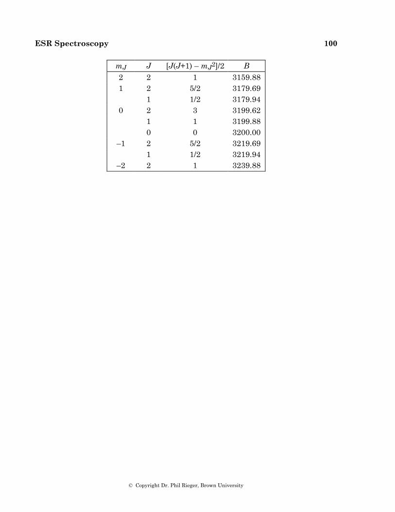
ESR Spectroscopy 100


mJ J [J(J+1) – mJ2]/2 B 2 2 1 3159.88 1 2 5/2 3179.69 1 1/2 3179.94

0 2 3 3199.62 1 1 3199.88 0 0 3200.00

–1 2 5/2 3219.69 1 1/2 3219.94

–2 2 1 3239.88

Date post:	10-Apr-2018
Category:	Documents
Upload:	dothien
View:	225 times
Download:	3 times

Electron Spin Resonance - Факультет Естественных...

Documents