Electron Spin Resonance Tutorialphys.ubbcluj.ro/~vchis/lab/esr1.pdf · Electron Spin Resonance 1....

Electron Spin Resonance

1. IntroductionElectron spin resonance (ESR) spectroscopy has been used for over 50 years to study a variety ofparamagnetic species. Here, we will focus on the spectra of organic and organotransition metal radicalsand coordination complexes. Although ESR spectroscopy is supposed to be a mature field with a fullydeveloped theory [1], there have been some surprises as organometallic problems have explored newdomains in ESR parameter space. We will start with a synopsis of the fundamentals of ESR spectroscopy.For further details on the theory and practice of ESR spectroscopy, refer to one of the excellent texts onESR spectroscopy [2-9].

The electron spin resonancespectrum of a free radical orcoordination complex with oneunpaired electron is the simplestof all forms of spectroscopy.The degeneracy of the electronspin states characterized by thequantum number, mS = ±1/2, islifted by the application of amagnetic field and transitionsbetween the spin levels areinduced by radiation of theappropriate frequency, as shownin Figure 1.1. If unpairedelectrons in radicals wereindistinguishable from freeelectrons, the only informationcontent of an ESR spectrumwould be the integratedintensity, proportional to theradical concentration.Fortunately, an un-pairedelectron interacts with itsenvironment, and the details ofESR spectra depend on thenature of those interactions.

Figure 1.1. Energy levels of an electron placed in a magnetic field. Thearrow shows the transitions induced by 0.315 cm-1 radiation.

There are two kinds of environmental interactions which are commonly important in the ESR spectrum ofa free radical:

To the extent that the unpaired electron has unquenched orbital angular momentum, the totalmagnetic moment is different from the spin-only moment (either larger or smaller, depending onhow the angular momentum vectors couple). It is customary to lump the orbital and spin angular

1.

Electron Spin Resonance Tutorial

http://www.chm.bris.ac.uk/emr/Phil/Phil_1/p_1.html (1 of 10) [10/2/2002 2:54:20 PM]

momenta together in an effective spin and to treat the effect as a shift in the energy of the spintransition.

The electron spin energy levels are split by interaction with nuclear magnetic moments – the nuclearhyperfine interaction. Each nucleus of spin I splits the electron spin levels into (2I + 1) sublevels.Since transitions are observed between sublevels with the same values of mI, nuclear spin splittingof energy levels is mirrored by splitting of the resonance line.

2.

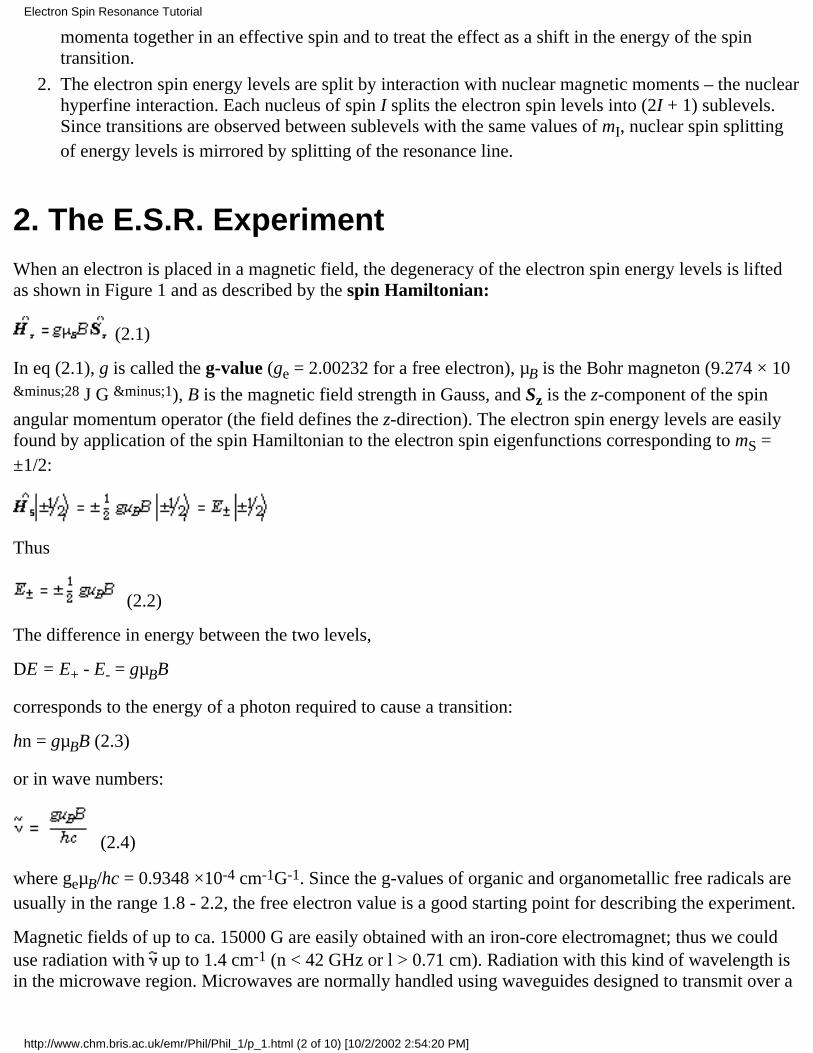
2. The E.S.R. ExperimentWhen an electron is placed in a magnetic field, the degeneracy of the electron spin energy levels is liftedas shown in Figure 1 and as described by the spin Hamiltonian:

(2.1)

In eq (2.1), g is called the g-value (ge = 2.00232 for a free electron), µB is the Bohr magneton (9.274 × 10−28 J G −1), B is the magnetic field strength in Gauss, and Sz is the z-component of the spinangular momentum operator (the field defines the z-direction). The electron spin energy levels are easilyfound by application of the spin Hamiltonian to the electron spin eigenfunctions corresponding to mS =±1/2:

Thus

(2.2)

The difference in energy between the two levels,

DE = E+ - E- = gµBB

corresponds to the energy of a photon required to cause a transition:

hn = gµBB (2.3)

or in wave numbers:

(2.4)

where geµB/hc = 0.9348 ×10-4 cm-1G-1. Since the g-values of organic and organometallic free radicals areusually in the range 1.8 - 2.2, the free electron value is a good starting point for describing the experiment.

Magnetic fields of up to ca. 15000 G are easily obtained with an iron-core electromagnet; thus we coulduse radiation with up to 1.4 cm-1 (n < 42 GHz or l > 0.71 cm). Radiation with this kind of wavelength isin the microwave region. Microwaves are normally handled using waveguides designed to transmit over a



relatively narrow frequency range. Waveguides look like rectangular cross-section pipes with dimensionson the order of the wavelength to be transmitted. As a practical matter, waveguides can't be too big or toosmall – 1 cm is a bit small and 10 cm a bit large; the most common choice, called X-band microwaves, hasl in the range 3.0 - 3.3 cm (n ˜ 9 - 10 GHz); in the middle of X-band, the free electron resonance is foundat 3390 G.

Although X-band is by far the most common, ESR spectrometers are available commercially in severalfrequency ranges:

Designation n/GHz l/cm B(electron)/Tesla

S 3.0 10.0 0.107

X 9.5 3.15 0.339

K 23 1.30 0.82

Q 35 0.86 1.25

W 95 0.315 3.3

Sensitivity

As for any quantum mechanical system interacting with electromagnetic radiation, a photon can induceeither absorption or emission. The experiment detects net absorption, i.e., the difference between thenumber of photons absorbed and the number emitted. Since absorption is proportional to the number ofspins in the lower level and emission is proportional to the number of spins in the upper level, netabsorption is proportional to the difference:

Net Absorptionµ N– – N+

The ratio of populations at equilibrium is given by the Boltzmann distribution:

(2.5)

For ordinary temperatures and ordinary magnetic fields, the exponent is very small and the exponentialcan be accurately approximated by the expansion, e–x ˜ 1 – x. Thus:

Since N– ˜N+ ˜ N/2, the population difference can be written



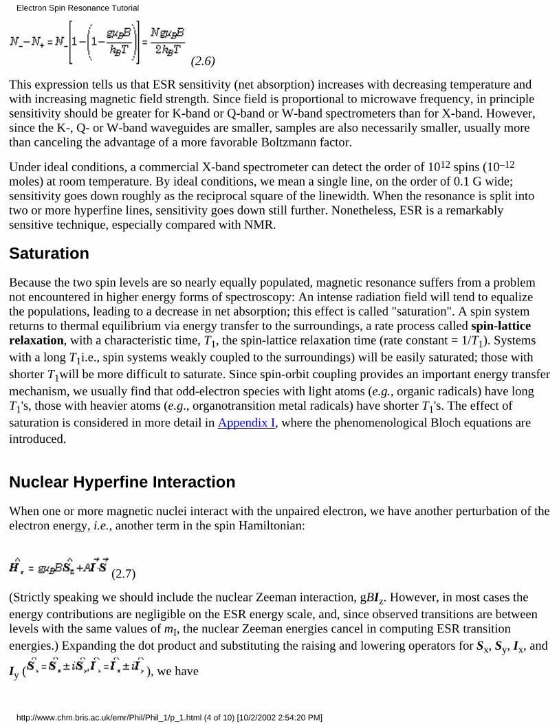
(2.6)

This expression tells us that ESR sensitivity (net absorption) increases with decreasing temperature andwith increasing magnetic field strength. Since field is proportional to microwave frequency, in principlesensitivity should be greater for K-band or Q-band or W-band spectrometers than for X-band. However,since the K-, Q- or W-band waveguides are smaller, samples are also necessarily smaller, usually morethan canceling the advantage of a more favorable Boltzmann factor.

Under ideal conditions, a commercial X-band spectrometer can detect the order of 1012 spins (10–12

moles) at room temperature. By ideal conditions, we mean a single line, on the order of 0.1 G wide;sensitivity goes down roughly as the reciprocal square of the linewidth. When the resonance is split intotwo or more hyperfine lines, sensitivity goes down still further. Nonetheless, ESR is a remarkablysensitive technique, especially compared with NMR.

Saturation

Because the two spin levels are so nearly equally populated, magnetic resonance suffers from a problemnot encountered in higher energy forms of spectroscopy: An intense radiation field will tend to equalizethe populations, leading to a decrease in net absorption; this effect is called "saturation". A spin systemreturns to thermal equilibrium via energy transfer to the surroundings, a rate process called spin-latticerelaxation, with a characteristic time, T1, the spin-lattice relaxation time (rate constant = 1/T1). Systemswith a long T1i.e., spin systems weakly coupled to the surroundings) will be easily saturated; those withshorter T1will be more difficult to saturate. Since spin-orbit coupling provides an important energy transfermechanism, we usually find that odd-electron species with light atoms (e.g., organic radicals) have longT1's, those with heavier atoms (e.g., organotransition metal radicals) have shorter T1's. The effect ofsaturation is considered in more detail in Appendix I, where the phenomenological Bloch equations areintroduced.

Nuclear Hyperfine Interaction

When one or more magnetic nuclei interact with the unpaired electron, we have another perturbation of theelectron energy, i.e., another term in the spin Hamiltonian:

(2.7)

(Strictly speaking we should include the nuclear Zeeman interaction, gBIz. However, in most cases theenergy contributions are negligible on the ESR energy scale, and, since observed transitions are betweenlevels with the same values of mI, the nuclear Zeeman energies cancel in computing ESR transitionenergies.) Expanding the dot product and substituting the raising and lowering operators for Sx, Sy, Ix, and

Iy ( ), we have



http://www.chm.bris.ac.uk/emr/Phil/Appendix_1.html

(2.8)

Suppose that the nuclear spin is 1/2; operating on the spin functions, we get:

The Hamiltonian matrix thus is

(2.9)

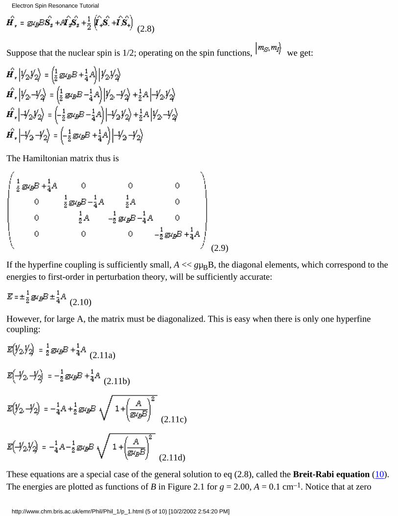
If the hyperfine coupling is sufficiently small, A << gµBB, the diagonal elements, which correspond to theenergies to first-order in perturbation theory, will be sufficiently accurate:

(2.10)

However, for large A, the matrix must be diagonalized. This is easy when there is only one hyperfinecoupling:

(2.11a)

(2.11b)

(2.11c)

(2.11d)

These equations are a special case of the general solution to eq (2.8), called the Breit-Rabi equation (10).The energies are plotted as functions of B in Figure 2.1 for g = 2.00, A = 0.1 cm–1. Notice that at zero



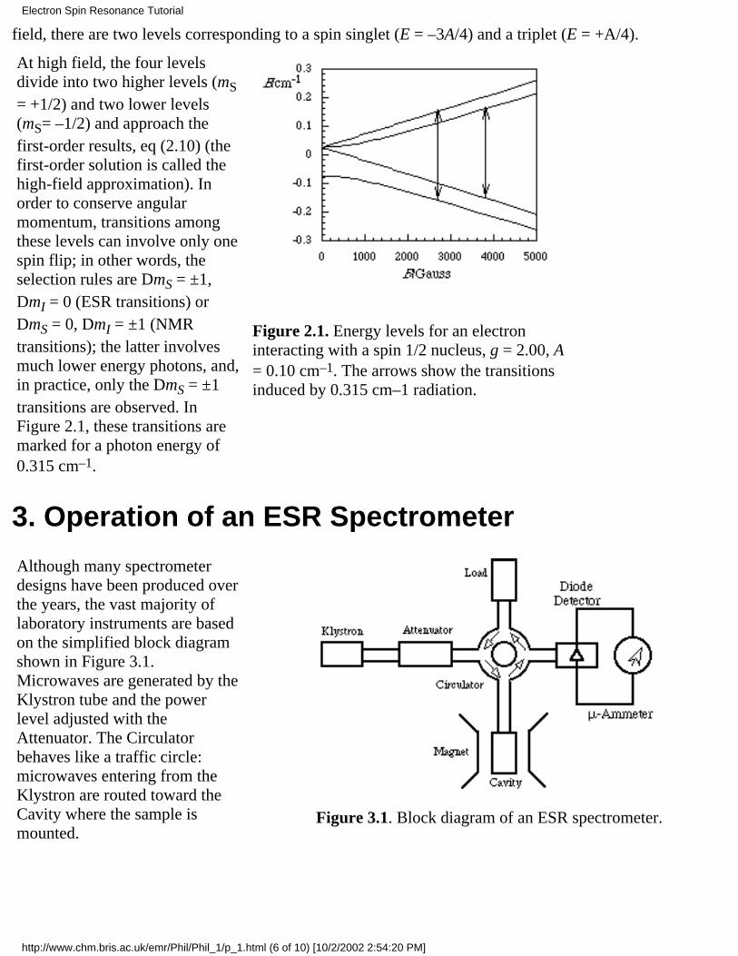
field, there are two levels corresponding to a spin singlet (E = –3A/4) and a triplet (E = +A/4).

At high field, the four levelsdivide into two higher levels (mS= +1/2) and two lower levels(mS= –1/2) and approach thefirst-order results, eq (2.10) (thefirst-order solution is called thehigh-field approximation). Inorder to conserve angularmomentum, transitions amongthese levels can involve only onespin flip; in other words, theselection rules are DmS = ±1,DmI = 0 (ESR transitions) orDmS = 0, DmI = ±1 (NMRtransitions); the latter involvesmuch lower energy photons, and,in practice, only the DmS = ±1transitions are observed. InFigure 2.1, these transitions aremarked for a photon energy of0.315 cm–1.

Figure 2.1. Energy levels for an electroninteracting with a spin 1/2 nucleus, g = 2.00, A= 0.10 cm–1. The arrows show the transitionsinduced by 0.315 cm–1 radiation.

3. Operation of an ESR Spectrometer

Although many spectrometerdesigns have been produced overthe years, the vast majority oflaboratory instruments are basedon the simplified block diagramshown in Figure 3.1.Microwaves are generated by theKlystron tube and the powerlevel adjusted with theAttenuator. The Circulatorbehaves like a traffic circle:microwaves entering from theKlystron are routed toward theCavity where the sample ismounted.

Figure 3.1. Block diagram of an ESR spectrometer.



Microwaves reflected back from the cavity (less when power is being absorbed) are routed tothe diode detector, and any power reflected from the diode is absorbed completely by the Load.The diode is mounted along the E-vector of the plane-polarized microwaves and thus produces acurrent proportional to the microwave power reflected from the cavity. Thus, in principle, theabsorption of microwaves by the sample could be detected by noting a decrease in current in themicroammeter. In practice, of course, such a d.c. measurement would be far too noisy to beuseful.

The solution to the signal-to-noise ratioproblem is to introduce small amplitude fieldmodulation. An oscillating magnetic field issuper-imposed on the d.c. field by means ofsmall coils, usually built into the cavity walls.When the field is in the vicinity of a resonanceline, it is swept back and forth through part ofthe line, leading to an a.c. component in thediode current. This a.c. component is amplifiedusing a frequency selective amplifier, thuseliminating a great deal of noise. Themodulation amplitude is normally less than theline width. Thus the detected a.c. signal isproportional to the change in sampleabsorption. As shown in Figure 3.2, thisamounts to detection of the first derivative ofthe absorption curve Figure 3.2.Small-amplitude field modulation

converts absorption curve to first-derivative.

Figure 3.3. First-derivative curves show betterapparent resolution than do absorption curves.

It takes a little practice to get used to looking atfirst-derivative spectra, but there is a distinctadvantage: first-derivative spectra have muchbetter apparent resolution than do absorptionspectra. Indeed, second-derivative spectra areeven better resolved (though thesignal-to-noise ratio decreases on furtherdifferentiation).



The microwave-generating klystron tuberequires a bit of explanation. A schematicdrawing of the klystron is shown in Figure 3.3.There are three electrodes: a heated cathodefrom which electrons are emitted, an anode tocollect the electrons, and a highly negativereflector electrode which sends those electronswhich pass through a hole in the anode back tothe anode.

Figure 3.3. Schematic drawing of amicrowave-generating klystron tube.

The motion of the charged electrons from the hole in the anode to the reflector and back to theanode generates a oscillating electric field and thus electromagnetic radiation. The transit timefrom the hole to the reflector and back again corresponds to the period of oscillation (1/n). Thusthe microwave frequency can be tuned (over a small range) by adjusting the physical distancebetween the anode and the reflector or by adjusting the reflector voltage. In practice, bothmethods are used: the metal tube is distorted mechanically to adjust the distance (a coarsefrequency adjustment) and the reflector voltage is adjusted as a fine control.

Figure 3.4. Microwave cavity.

Figure 3.5. Klystron mode and cavity dip.

The sample is mounted in the microwavecavity, shown in Figure 3.4. The cavity is arectangular metal box, exactly onewavelength in length. An X-band cavity hasdimensions of about 1 ×2 ×3 cm. Theelectric and magnetic fields of the standingwave are shown in the figure. Note that thesample is mounted in the electric field nodalplane, but at a maximum in the magneticfield.

Since the cavity length is not adjustable butit must be exactly one wavelength, thespectrometer must be tuned such that theklystron frequency is equal to the cavityresonant frequency. The tune-up procedureusually includes observing the klystronpower mode. That is, the klystron reflectorvoltage is swept, and the diode current isplotted on an oscilloscope or other device.When the klystron frequency is close to the

cavity resonant frequency, much less power is reflected from the cavity to the diode, resulting ina dip in the power mode as shown in Figure 3.5. The "cavity dip" is centered on the power modeusing the coarse mechanical frequency adjustment with the reflector voltage used to fine tunethe frequency.



4. Isotropic ESR SpectraAn isotropic ESR spectrum& #150; the spectrum of a freely tumbling radical in liquid solution& #150;can contain several kinds of chemically useful information:

The hyperfine coupling pattern provides information on the numbers and kinds of magnetic nucleiwith which the unpaired electron interacts.

1.

The spacing of the lines and the center of gravity of the spectrum yield the hyperfine couplingconstants, <AS> and g-value, <g>, which are related to the way in which the unpaired electron spindensity is distributed in the molecule.

2.

The integrated intensity of the spectrum is proportional to the concentration of radicals in thesample.

3.

The spectral linewidths are related to the rate of the rotational motions which average anisotropiesin the g- and hyperfine matrices (see §5) and to the rates of fluxional processes which averagenuclear positions in a radical.

4.

The saturation behavior of a spectrum – the variation of integrated intensity with microwave power– is related to the spin-lattice relaxation time, a measure of the rate of energy transfer between theelectron spin and its surroundings.

5.

The degree to which these kinds of information have been exploited varies widely. Althoughexperimentalists often make qualitative observations relating "strong" or "weak" spectra to chemicalcircumstances, quantitative applications of integrated intensities are rare in ESR studies. This could be auseful analytical approach in some cases. The interested reader is referred to Wertz and Bolton [5], whodiscuss the technique, point out the variables which must be controlled, and suggest intensity standards.

Largely because spin-orbit coupling results in spin state admixture, electronic spin-lattice relaxation timesare normally short for species containing heavy atoms such as transition metals. This has twoconsequences. Short relaxation times mean that saturation problems, which plague ESR spectroscopistsstudying organic radicals and NMR spectroscopists in general, are largely absent in organometallic ESRstudies. Thus spectra ordinarily can be recorded at full microwave power with salutary consequences forsensitivity. On the other hand, relaxation times are most easily determined by measuring spectral intensityas a function of microwave power in the saturation region. If relaxation times are short, very high power isrequired, out of the range of operation of most spectrometers.

Line Positions in Isotropic Spectra

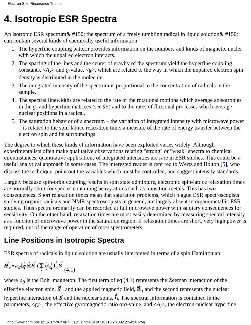
ESR spectra of radicals in liquid solution are usually interpreted in terms of a spin Hamiltonian

(4.1)

where µB is the Bohr magneton. The first term of eq (4.1) represents the Zeeman interaction of the

effective electron spin, , and the applied magnetic field, , and the second represents the nuclear

hyperfine interaction of and the nuclear spins, . The spectral information is contained in theparameters, <g> , the effective gyromagnetic ratio org-value, and <AI>, the electron-nuclear hyperfine



coupling constant for nucleus i. Using spin functions based on the quantum numbers mS and mi, eq (4.1)can be used to compute energy levels. Equating energy differences for the allowed transitions (DmS = ±1,Dmi = 0) with the microwave photon energy,

E(mS = 1/2) − E(mS = −1/2) = hn (4.2)

the resonant magnetic field can be predicted. To first-order in perturbation theory, the resonant field is

(4.3)

where B0 = hn/<g>µB represents the center of the spectrum and <ai> = <AS>/<g> µB is the hyperfinecoupling constant in field units.

The coupling constant in eq(4.1) has energy units, but the energies are very small so that frequency (MHz)or wave number (10-4 cm-1) units are more commonly used. Even more often, however, isotropic couplingconstants are given in units of magnetic field strength, usually gauss, though SI purists sometimes usemillitesla (1 mT = 10 G). Conversions from units of gauss to frequency or wave number units involves theg-value

<A>/MHz = 2.8025 (<g>/ge) <a>/G (4.4a)

<A>/10–4 cm–1 = 0.93480 (<g>/ge) <a>/G (4.4b)

Note that coupling constants in 10–4 cm–1 are comparable in magnitude to those expressed in gauss.Although the units used for isotropic hyperfine coupling constants is largely a matter of taste, thecomponents of an anisotropic hyperfine coupling matrix (see §5) should be given in frequency or wavenumber units unless the g-matrix is virtually isotropic

(continued)



Hyperfine Coupling Patterns

Nuclear hyperfine coupling results in a multi-line ESR spectrum, analogous to the spin-spin couplingmultiplets of NMR spectra. ESR spectra are simpler to understand than NMR spectra in thatsecond-order effects normally do not alter the intensities of components; on the other hand, ESRmultiplets can be much more complex when the electron interacts with several high-spin nuclei, and, aswe will see below, there can be considerable variation in linewidth within a spectrum.

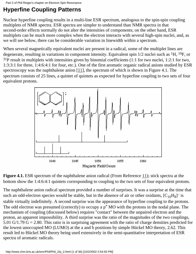
When several magnetically equivalent nuclei are present in a radical, some of the multiplet lines aredegenerate, resulting in variations in component intensity. Equivalent spin 1/2 nuclei such as 1H, 19F, or31P result in multiplets with intensities given by binomial coefficients (1:1 for two nuclei, 1:2:1 for two,1:3:3:1 for three, 1:4:6:4:1 for four, etc.). One of the first aromatic organic radical anions studied by ESRspectroscopy was the naphthalene anion [11], the spectrum of which is shown in Figure 4.1. Thespectrum consists of 25 lines, a quintet of quintets as expected for hyperfine coupling to two sets of fourequivalent protons.

Figure 4.1. ESR spectrum of the naphthalene anion radical (From Reference 11); stick spectra at thebottom show the 1:4:6:4:1 quintets corresponding to coupling to the two sets of four equivalent protons.

The naphthalene anion radical spectrum provided a number of surprises. It was a surprise at the time thatsuch an odd-electron species would be stable, but in the absence of air or other oxidants, [C10H8]– isstable virtually indefinitely. A second surprise was the appearance of hyperfine coupling to the protons.The odd electron was presumed (correctly) to occupy a p* MO with the protons in the nodal plane. Themechanism of coupling (discussed below) requires "contact" between the unpaired electron and theproton, an apparent impossibility. A third surprise was the ratio of the magnitudes of the two couplings,5.01 G/1.79 G = 2.80. This ratio is in surprising agreement with the ratio of charge densities predicted forthe lowest unoccupied MO (LUMO) at the a and b positions by simple Hückel MO theory, 2.62. Thisresult led to Hückel MO theory being used extensively in the semi-quantitative interpretation of ESRspectra of aromatic radicals.

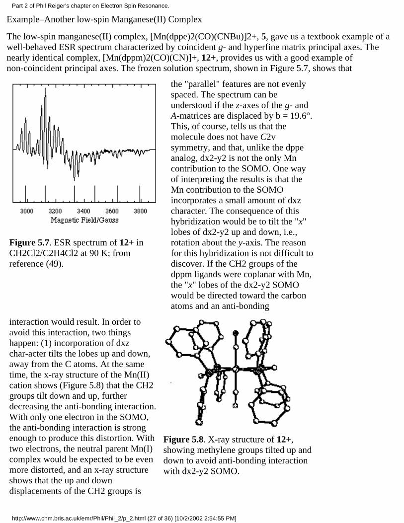
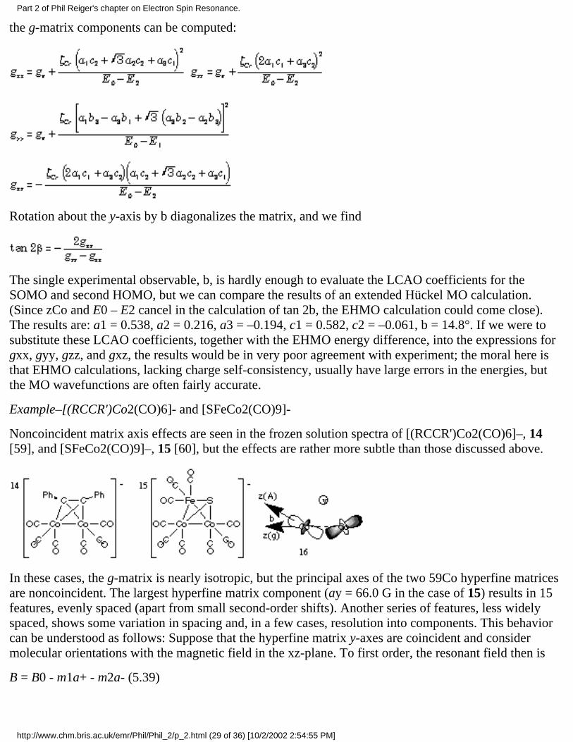
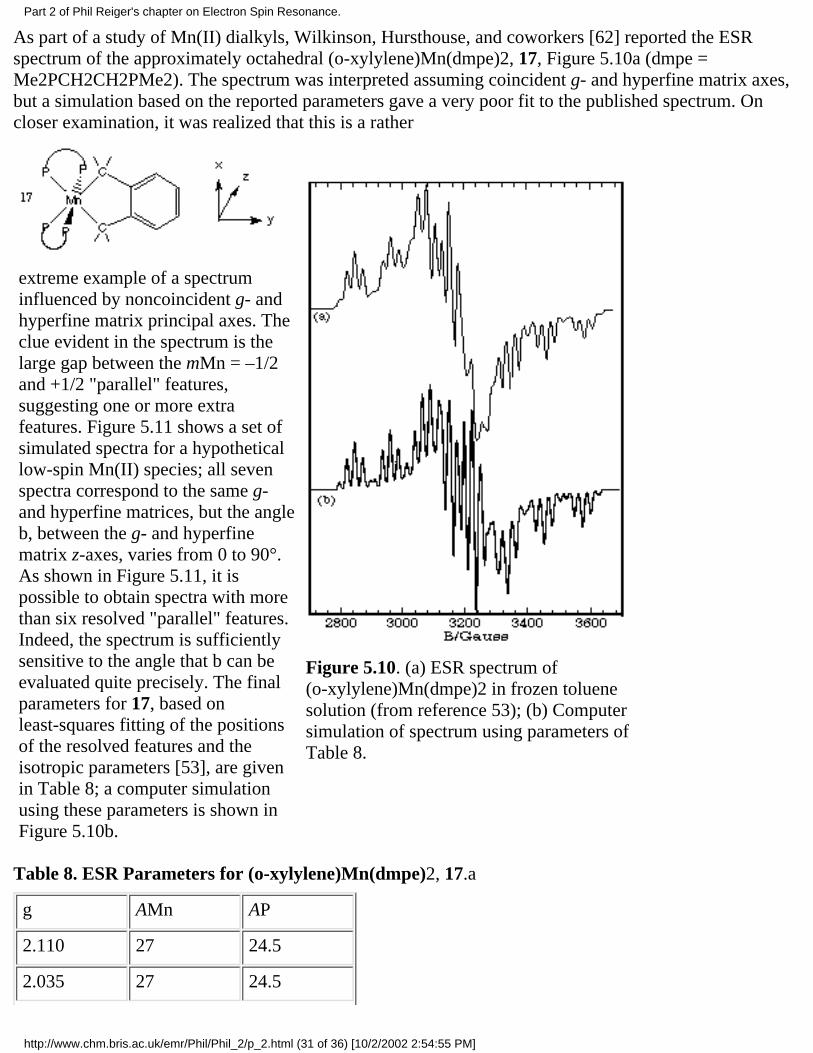
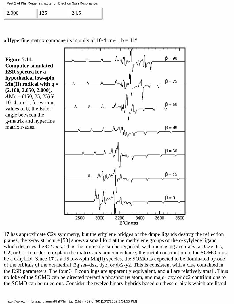
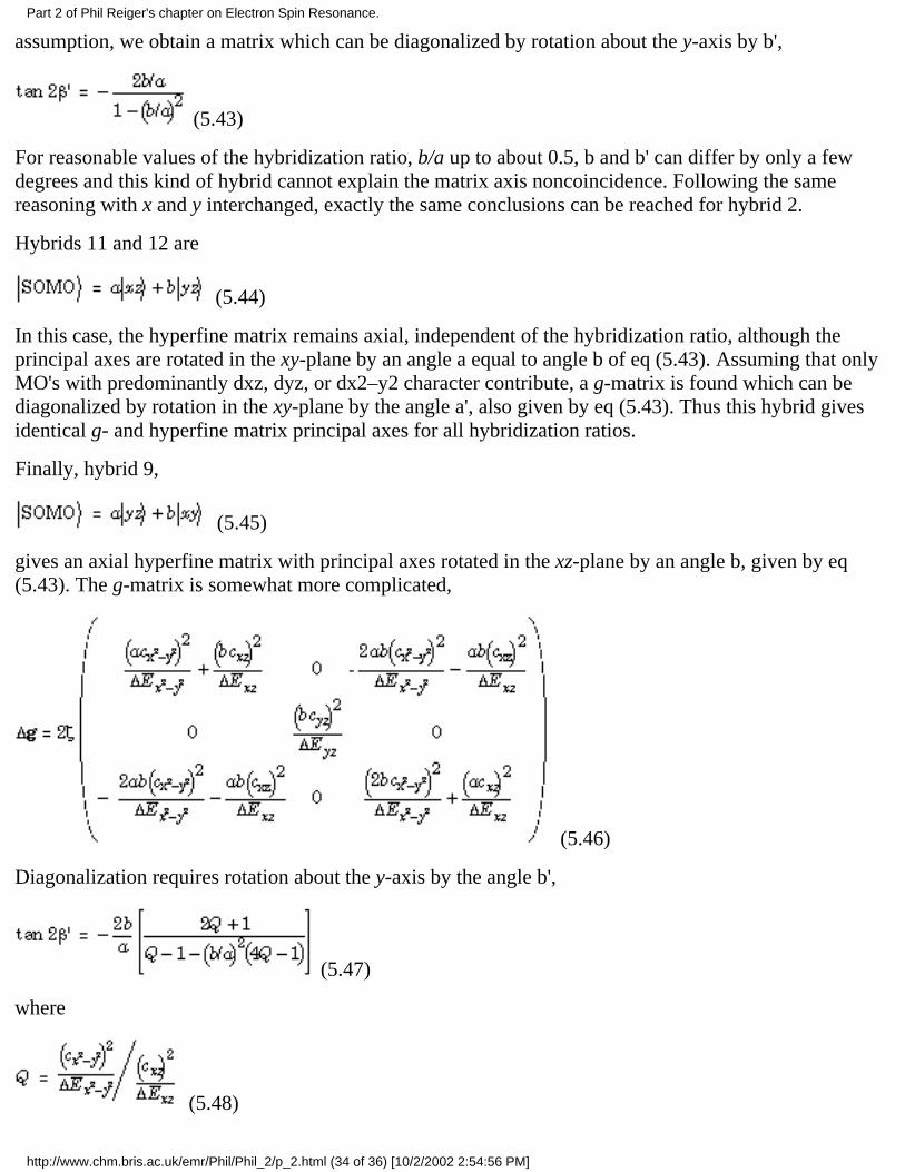
Part 2 of Phil Reiger's chapter on Electron Spin Resonance.


Just as in NMR, a multiplet pattern gives an important clue to the identity of a radical. For example, theseries of radicals derived from the nucleophilic displacement of Co(CO)4

– from [(RCCR')Co2(CO)6– by

CO, phosphines, or phosphites was identified in large part from the resulting hyperfine patterns [12].Depending on the nucleophile, spectra were observed which showed coupling to 0, 1, 2, or 3 31P nuclei,but always to a single 59Co nucleus. The parameters <g> and aCo were found to depend slightly on thesubstituents on the acetylene moiety, suggesting that the acetylene was retained in the radical, butotherwise the parameters were nearly constant over the series, suggesting a single family of radicals. Theappearance of 0 - 3 phosphorus couplings suggested three additional ligands, either CO or a phosphine orphosphite. Taken together, this information identified the radicals as (RCCR')CoL3, where L = CO, PR3,or P(OR)3. Figure 4.2(a) shows the experimental first-derivative spectrum of (Ph2C2)Co(CO)2P(OMe)3,

1, and Figure 4.2(c) shows a first-order "stick spectrum" showing the line positions ( <g> = 2.061, aCo =45.2 G, aP = 176.2 G). Hyperfine coupling to 59Co (I = 7/2) and 31P (I = 1/2) nuclei results in an octet ofdoublets. The spectrum is somewhat complicated by the obvious variation in linewidth, but theassignments are quite straightforward.

Figure 4.2. (a) Isotropic ESR spectrum of (Ph2C2)Co(CO)2P(OMe)3(1) in THF solution at 260 K (fromreference 12); (b) Second-order "stick spectrum"; (c) First-order "stick spectrum".

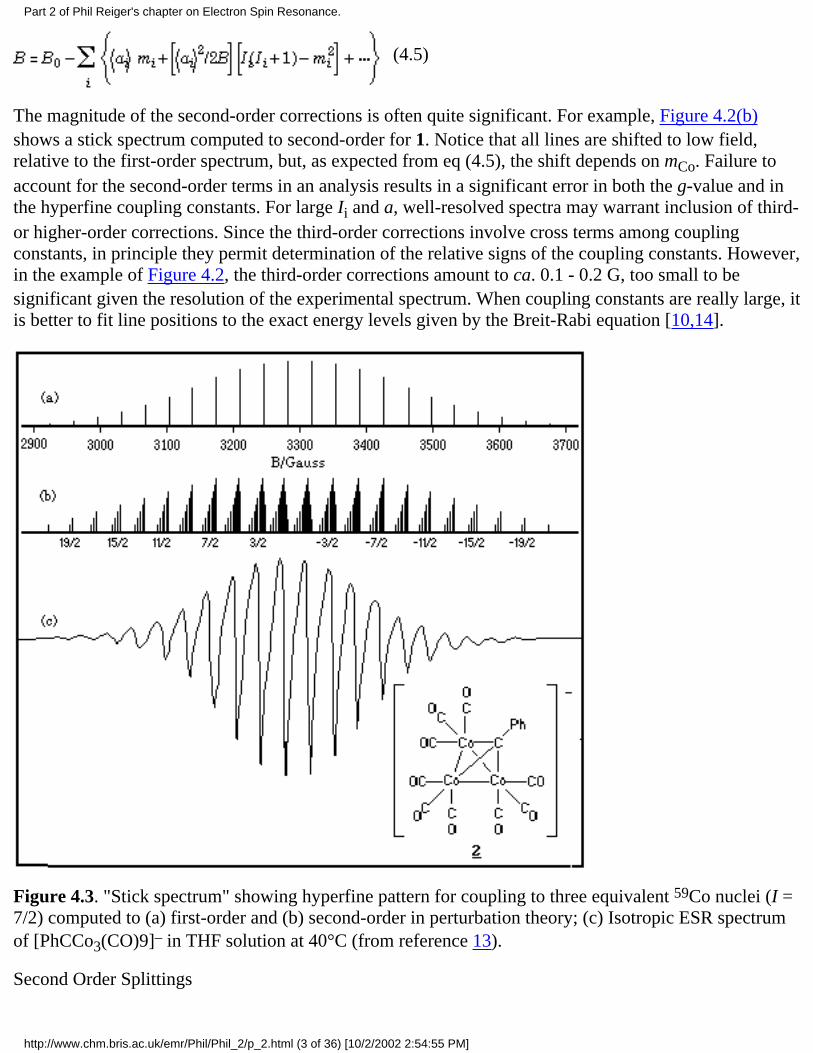
Nuclei with I > 1/2 give less familiar multiplet intensity ratios. Thus, for example, three equivalent 59Conuclei (I = 7/2) give (to first order) 22 lines with intensity ratios 1:3:6:10:15:21:28:36:42:46:48:48:46...,as shown in Figure 4.3(a). The experimental spectrum of [PhCCo3(CO)9]–, 2 [13], which shows thiscoupling pattern, is given in Figure 4.3(c).

Spin Hamiltonian Parameters from Spectra

Once a hyperfine pattern has been recognized, the line position information can be summarized by thespin Hamiltonian parameters, <g> and <a>. These parameters can be extracted from spectra by a linearleast-squares fit of experimental line positions to eq (4.3). However, for high-spin nuclei and/or largecouplings, one soon finds that the lines are not evenly spaced as predicted by eq (4.3) and second-ordercorrections must be made. Solving the spin Hamiltonian, eq (4.1), to second order in perturbation theory,eq (4.3) becomes



(4.5)

The magnitude of the second-order corrections is often quite significant. For example, Figure 4.2(b)shows a stick spectrum computed to second-order for 1. Notice that all lines are shifted to low field,relative to the first-order spectrum, but, as expected from eq (4.5), the shift depends on mCo. Failure toaccount for the second-order terms in an analysis results in a significant error in both the g-value and inthe hyperfine coupling constants. For large Ii and a, well-resolved spectra may warrant inclusion of third-or higher-order corrections. Since the third-order corrections involve cross terms among couplingconstants, in principle they permit determination of the relative signs of the coupling constants. However,in the example of Figure 4.2, the third-order corrections amount to ca. 0.1 - 0.2 G, too small to besignificant given the resolution of the experimental spectrum. When coupling constants are really large, itis better to fit line positions to the exact energy levels given by the Breit-Rabi equation [10,14].

Figure 4.3. "Stick spectrum" showing hyperfine pattern for coupling to three equivalent 59Co nuclei (I =7/2) computed to (a) first-order and (b) second-order in perturbation theory; (c) Isotropic ESR spectrumof [PhCCo3(CO)9]– in THF solution at 40°C (from reference 13).

Second Order Splittings



Equation (4.5) describes line positions correctly for spectra with hyperfine coupling to two or morenuclei provided that the nuclei are not magnetically equivalent. When two or more nuclei are completelyequivalent, i.e., both instantaneously equivalent and equivalent over a time average, then the nuclearspins should be described in terms of the total nuclear spin quantum numbers J and mJ rather than theindividual Ii and mi. In this "coupled representation", the degeneracies of some multiplet lines are liftedwhen second-order shifts are included. This can lead to extra lines and/or asymmetric line shapes. Theeffect was first observed in the spectrum of the methyl radical, CH3. The three equivalent protons lead toa nondegenerate nuclear spin state with J = 3/2 (m = ±3/2, ±1/2) and a two-fold degenerate state with J =1/2 (m = ±1/2). Thus six hyperfine lines are observed under conditions of high resolution, as shown inFigure 4.4

Figure 4.4. ESR spectrum of the methyl radical, CH3(from reference 15; note discontinuities in magneticfield axis).

Another example is the spectrum of a tricobaltcarbon radical anion, where the three equivalent spin 7/259Co nuclei should be described in terms of 11 J-states with J ranging from 21/2 to 1/2. The mJ = 17/2feature, for example, has three components with J = 21/2, 19/2, and 17/2, degeneracies of 1, 2, and 3, andsecond-order shifts of 97 <a>2/4B, 55 <a>2/4B, and 17 <a>2/4B, respectively. The shifts are too small tobe resolved, but they lead to an asymmetric absorption line envelope with apparent broadening on thelow-field side, as shown in Figure 4.3(a) and as is observed in the experimental spectrum of 2, shown inFigure 4.3(c) [13].

Interpretation of Isotropic Parameters

When ESR spectra were obtained for the benzene anion radical, [C6H6]–, and the methyl radical, CH3,the proton hyperfine coupling constants were found to be 3.75 G and 23.0 G, respectively. Since eachcarbon atom of the benzene anion carries an electron spin density of 1/6, the two results suggest that theproton coupling to an electron in a p* orbital is proportional to the spin density on the adjacent carbonatom,

<a> = QCHH rCp (4.6)



where the parameter QCHH = 23.0 G, based on CH3, 22.5 G, based on [C6H6]–, or 23.7 G, based on avalence-bond theoretical calculation [16]. An isotropic hyperfine coupling to H can only arise throughthe so-called Fermi contact interaction of the unpaired electron with the H nucleus, and this is symmetryforbidden for organic p-radicals where the H nuclei lie in the plane of symmetry. The interaction arises ina slightly more complicated way: "spin polarization". As shown in Figure 4.5, the C 2pz orbital has zeroprobability at the H nucleus, but there is significant overlap of the C 2pz and H 1s orbitals, Suppose the H1s orbital is part of a s-bonding MO and the C 2pz part of the singly-occupied p* MO. In the overlapregion of these two MO's, there is a tendency for the unpaired spin in the SOMO to polarize the pair ofelectrons in bonding MO such that the spins in the overlap region are parallel, necessarily leaving anoppositely oriented spin near the H nucleus.

Figure 4.5. Schematic representation of spinpolarization of a C-H s-orbital by electron spinin a p* orbital. Note that the polarization effectis far from complete; only a tiny fraction of theelectron density near the H nucleus is excessspin-down.

It is sometimes assumed that there is a relation analogous to eq (4.6) for metal or ligand hyperfinecouplings in spectra of organometallic radicals. Such an assumption is usually unwarranted. An isotropichyperfine coupling has three contributions:

Fermi contact interaction between the nuclear spin and electron spin density in the valence-shells-orbital

1.

Fermi contact interaction between the nuclear spin and spin density in inner-shell s-orbitals arisingfrom spin polarization by unpaired electron density in valence-shell p- or d-orbitals

2.

a contribution from spin-orbit coupling.3.

The first contribution is positive (for a positive nuclear magnetic moment), the second is normallynegative, and the third may be of either sign. Because direct involvement of hydrogen 1s character in theSOMO of an organic p-radical is symmetry-forbidden and spin-orbit coupling is negligible incarbon-based radicals, proton couplings in such radicals result solely from spin polarization and thus areproportional to the polarizing spin density. All three contributions are usually significant fororganometallic radicals. Although there are a few cases where polarization constants, analogous toQCHH, have been estimated [17], they are of use only in a more complete analysis based on the results ofa solid state ESR study.

As we will see below, g-matrices are often difficult to interpret reliably. The interpretation of isotropicg-values is even more dangerous. Thus isotropic ESR spectra should be used to characterize a radical bymeans of the hyperfine coupling pattern, to study its dynamical properties through linewidth effects, or tomeasure its concentration by integration of the spectrum and comparison with an appropriate standard,but considerable caution should be exercised in interpreting the g-value or nuclear hyperfine couplingconstants.



Linewidths in Isotropic Spectra

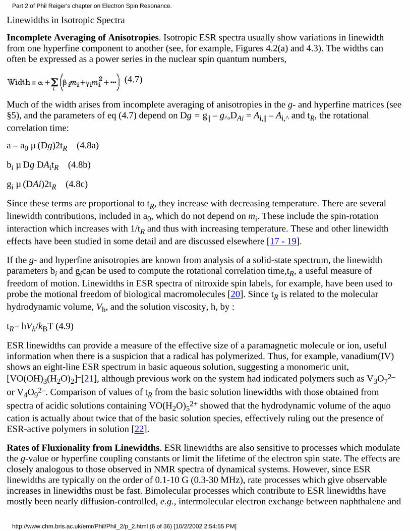
Incomplete Averaging of Anisotropies. Isotropic ESR spectra usually show variations in linewidthfrom one hyperfine component to another (see, for example, Figures 4.2(a) and 4.3). The widths canoften be expressed as a power series in the nuclear spin quantum numbers,

(4.7)

Much of the width arises from incomplete averaging of anisotropies in the g- and hyperfine matrices (see§5), and the parameters of eq (4.7) depend on Dg = g|| – g^,DAi = Ai,|| – Ai,^ and tR, the rotationalcorrelation time:

a – a0 µ (Dg)2tR (4.8a)

bi µ Dg DAitR (4.8b)

gi µ (DAi)2tR (4.8c)

Since these terms are proportional to tR, they increase with decreasing temperature. There are severallinewidth contributions, included in a0, which do not depend on mi. These include the spin-rotationinteraction which increases with 1/tR and thus with increasing temperature. These and other linewidtheffects have been studied in some detail and are discussed elsewhere [17 - 19].

If the g- and hyperfine anisotropies are known from analysis of a solid-state spectrum, the linewidthparameters bi and gican be used to compute the rotational correlation time,tR, a useful measure offreedom of motion. Linewidths in ESR spectra of nitroxide spin labels, for example, have been used toprobe the motional freedom of biological macromolecules [20]. Since tR is related to the molecularhydrodynamic volume, Vh, and the solution viscosity, h, by :

tR= hVh/kBT (4.9)

ESR linewidths can provide a measure of the effective size of a paramagnetic molecule or ion, usefulinformation when there is a suspicion that a radical has polymerized. Thus, for example, vanadium(IV)shows an eight-line ESR spectrum in basic aqueous solution, suggesting a monomeric unit,[VO(OH)3(H2O)2]–[21], although previous work on the system had indicated polymers such as V3O7

2–

or V4O92–. Comparison of values of tR from the basic solution linewidths with those obtained from

spectra of acidic solutions containing VO(H2O)52+ showed that the hydrodynamic volume of the aquo

cation is actually about twice that of the basic solution species, effectively ruling out the presence ofESR-active polymers in solution [22].

Rates of Fluxionality from Linewidths. ESR linewidths are also sensitive to processes which modulatethe g-value or hyperfine coupling constants or limit the lifetime of the electron spin state. The effects areclosely analogous to those observed in NMR spectra of dynamical systems. However, since ESRlinewidths are typically on the order of 0.1-10 G (0.3-30 MHz), rate processes which give observableincreases in linewidths must be fast. Bimolecular processes which contribute to ESR linewidths havemostly been nearly diffusion-controlled, e.g., intermolecular electron exchange between naphthalene and



its anion radical [23] and reversible axial ligation of square planar copper(II) complexes [24].

The effect of rate processes on linewidths can be understood quantitatively in terms of the modifiedBloch equations ([25], see also Appendix 3), or, more accurately, in terms of density matrix [26] orrelaxation matrix [18, 27] formalisms. If a rate process modulates a line position through an amplitudeDB (Dw in angular frequency units) by fluctuating between two states, each with lifetime t, a single lineis observed with an excess width proportional to (Dw)2t when t–1 >> Dw – the fast exchange limit. Asthe lifetime increases, the line broadens to indetectability and then re-emerges as two broad lines. Theseshift apart and sharpen until, in the slow exchange limit (t-1 << Dw), two lines are observed with widthsproportional to t-1.

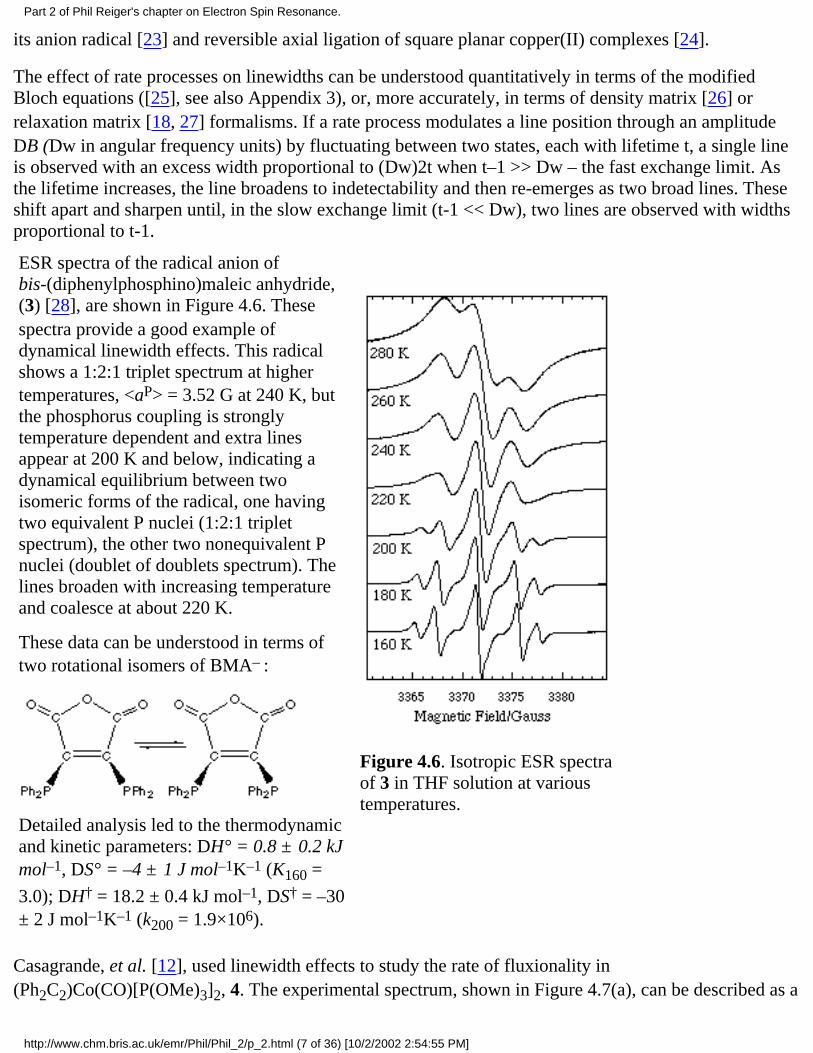
ESR spectra of the radical anion ofbis-(diphenylphosphino)maleic anhydride,(3) [28], are shown in Figure 4.6. Thesespectra provide a good example ofdynamical linewidth effects. This radicalshows a 1:2:1 triplet spectrum at highertemperatures, <aP> = 3.52 G at 240 K, butthe phosphorus coupling is stronglytemperature dependent and extra linesappear at 200 K and below, indicating adynamical equilibrium between twoisomeric forms of the radical, one havingtwo equivalent P nuclei (1:2:1 tripletspectrum), the other two nonequivalent Pnuclei (doublet of doublets spectrum). Thelines broaden with increasing temperatureand coalesce at about 220 K.

These data can be understood in terms oftwo rotational isomers of BMA– :

Detailed analysis led to the thermodynamicand kinetic parameters: DH° = 0.8 ± 0.2 kJmol–1, DS° = –4 ± 1 J mol–1K–1 (K160 =

3.0); DH† = 18.2 ± 0.4 kJ mol–1, DS† = –30± 2 J mol–1K–1 (k200 = 1.9×106).

Figure 4.6. Isotropic ESR spectraof 3 in THF solution at varioustemperatures.

Casagrande, et al. [12], used linewidth effects to study the rate of fluxionality in(Ph2C2)Co(CO)[P(OMe)3]2, 4. The experimental spectrum, shown in Figure 4.7(a), can be described as a



1:2:1 triplet of octets; the spectrum is complicated by a large linewidth dependence on mCo, but asdemonstrated in Figures 4.7(b) and 4.7(c), the central lines of the triplets are much broader than the outerlines. This radical has a distorted tetrahedral structure with the semi-occupied molecular orbital (SOMO)largely cobalt 3dz

2 in character [29]. Thus the ligand sites can be described as axial or equatorial relative

to the unique z-axis. Several isomers are possible, but the 31P couplings distinguish between the isomerwith an axial phosphite (ax,eq) and those with either CO or the acetylene axial and both phosphitesequatorial (eq,eq). The rate of interconversion between eq,eq and ax,eq isomers was estimated from therelative widths of the mP= ±1 and 0 lines, given the isotropic coupling constants for the various 31Pnuclei (which were determined from the frozen solution spectrum [29]). The average rate was found tobe approximately 2 ×1010 s–1 (Ea = 17 kJ mol–1) at 298 K.

Figure 3.7. ESR spectrum of (Ph2C2)Co(CO)[P(OMe)3]2 (a) Experimental spectrum of THF solution at290 K; (b and c) Computer-simulated spectra including (b) the mCoand mP linewidth dependence, and (c)the mCo linewidth dependence only.

5. Anisotropic ESR Spectra



The anisotropies which lead to line broadening in isotropic ESR spectra influence solid-state spectramore directly. Accordingly a more complex spin Hamiltonian is required to interpret such spectra

(5.1)

In eq (5.1), g and Ai are 3 × 3 matrices representing the anisotropic Zeeman and nuclear hyperfineinteractions. In general, a coordinate system can be found (the g-matrix principal axes) in which g isdiagonal. If g and Ai are diagonal in the same coordinate system, we say that their principal axes arecoincident.

In species with two or more unpaired electrons, a fine structure term must be added to the spinHamiltonian to represent electron spin-spin interactions. We will confine our attention here to radicalswith one unpaired electron (S = 1/2) but will address the S > 1/2 problem in Section 6.

Nuclear quadrupole interactions introduce line shifts and forbidden transitions in spectra of radicals withnuclei having I > 1/2. In practice, quadrupolar effects are observable only in very well-resolved spectraor in spectra of radicals with nuclei having small magnetic moments and large quadrupole moments. Themost extreme case of a small magnetic moment to quadrupole moment ratio is that of 191Ir/193Ir, andspectra of [Ir(CN)6]3– [30], [Ir(CN)5Cl]4– and [Ir(CN)4Cl2]4– [31], and

[Ir2(CO)2(PPh3)2(m-RNNNR)2]+, R = p-tolyl [32], show easily recognizable quadrupolar effects. Other

nuclei for which quadrupolar effects might be expected include 151Eu/153Eu, 155Gd/157Gd, 175Lu, 181Ta,189Os, and 197Au. When quadrupolar effects are important, it is usually necessary to take account of thenuclear Zeeman interaction as well. The nuclear quadrupole and nuclear Zeeman interactions add twomore terms to the spin Hamiltonian. Since these terms considerably complicate an already complexsituation, we will confine our attention here to nuclei for which quadrupolar effects can be neglected.

When a radical is oriented such that the magnetic field direction is located by the polar and azimuthalangles,q and f, relative to the g-matrix principal axes, the resonant field is given, to first order inperturbation theory, by [33]

(5.2) where (5.3)

g2 = gx2sin2qcos2f + gy

2sin2qsin2f+ gz2cos2q (5.4)

Ai2 = Aiz

2 Six2 + Aiy

2 Siy2 + Aiz2 Siz

2 (5.5)

Sik = [gxsin q cos f lixk + gysin q cos f liyk + gzcos q lizk]/g (5.6)

and the lijkare direction cosines indicating the orientation of the kth principal axis of the ith hyperfinematrix relative to the jth g-matrix principal axis. When the matrix principal axes are coincident, only oneof the lijk of eq (4.6) will be nonzero. When the hyperfine matrix components are large, second-order

terms [33] must be added to eq (5.2); these result in down-field shifts, proportional to mi2.

Solid-State ESR Spectra



So long as they are dilute (to avoid line broadening from intermolecular spin exchange), radicals can bestudied in the solid state as solutes in single crystals, powders, glasses or frozen solutions. Radicals canbe produced in situ by UV- or g-irradiation of a suitable precursor in a crystalline or glassy matrix. Whilemany organometallic radicals have been studied in this way [34], it is often easier to obtain solid stateESR spectra by freezing the liquid solution in which the radical is formed. A variety of techniques thencan be used to generate radicals, e.g., chemical reactions, electrochemical reduction or oxidation, orphotochemical methods. Furthermore, the radical is studied under conditions more closely approximatingthose in which its reaction chemistry is known.

Spectra of Dilute Single Crystals. Spectra of radicals in a dilute single crystal are obtained for a varietyof orientations, usually with the field perpendicular to one of the crystal axes. Spectra usually can beanalyzed as if they were isotropic to obtain an effective g-value and hyperfine coupling constants. Sincethe g- and hyperfine matrix principal axes are not necessarily the same as the crystal axes, the matrices,written in the crystal axis system usually will have off-diagonal elements. Thus, for example, if spectraare obtained for a variety of orientations in the crystal xy-plane, the effective g-value is

gf2 = (gxx cos f + gyx sin f)2 + (gxy cos f + gyy sin f)2 + (gxz cos f + gyz sin f)2 (5.7)

or gf2 = K1+ K2 cos 2f + K3 sin 2f (5.8)

where K1 = (gxx2 + gyy2 + gxz2 + gyz2 + 2 gxy2)/2 (5.9a)

K2 = (gxx2 - gyy2 + gxz2 - gyz2)/2 (5.9b)

K3 = gxy(gxx + gyy) + gxzgyz (5.9c)

A sinusoidal plot of gf2 vs f can be analyzed to determine K1, K2, and K3. Exploration of another crystalplane gives another set of K's which depend on other combinations of the gij; eventually enough data areobtained to determine the six independent gij (g is a symmetric matrix so that gij = gji). The g2-matrixthen is diagonalized to obtain the principal values and the transformation matrix, elements of which arethe direction cosines of the g-matrix principal axes relative to the crystal axes. An analogous treatment ofthe effective hyperfine coupling constants leads to the principal values of the A2-matrix and theorientation of its principal axes in the crystal coordinate system.

Analysis of Powder Spectra. Since ESR spectra are normally recorded as the first derivative ofabsorption vs. field, observable features in the spectrum of a powder correspond to molecular orientationsfor which the derivative is large in magnitude or changes in sign. For any spin Hamiltonian, there will beminimum and maximum resonant fields at which the absorption changes rapidly from zero, leading to alarge value of the derivative and features which resemble positive-going and negative-going absorptionlines. Peaks in the absorption envelope correspond to derivative sign changes and lead to featuresresembling isotropic derivative lines. The interpretation of a powder spectrum thus depends on theconnection of the positions of these features to the g- and hyperfine matrix components.

Early treatments of powder patterns attempted to deal with the spatial distribution of resonant fields byanalytical mathematics [35]. This approach led to some valuable insights but the algebra is much toocomplex when nonaxial hyperfine matrices are involved. Consider the simplest case: a single resonanceline without hyperfine structure. The resonant field is given by eq (5.3). Features in the first derivativespectrum correspond to discontinuities or turning points in the absorption spectrum which arise when¶B/¶q or ¶B/¶f are zero,



(5.10a)

or (5.10b)

These equations have three solutions: (i) q = 0; (ii) q= 90°, f = 0; and (iii) q = f = 90°. Since q and f are inthe g-matrix axis system, observable features are expected for those fields corresponding to orientationsalong the principal axes of the g-matrix. This being the case, the principal values of the g-matrix areobtained from a straightforward application of eq (5.3).

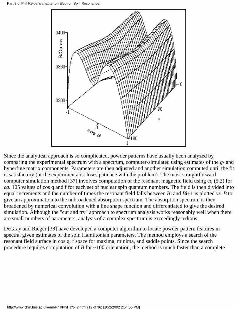
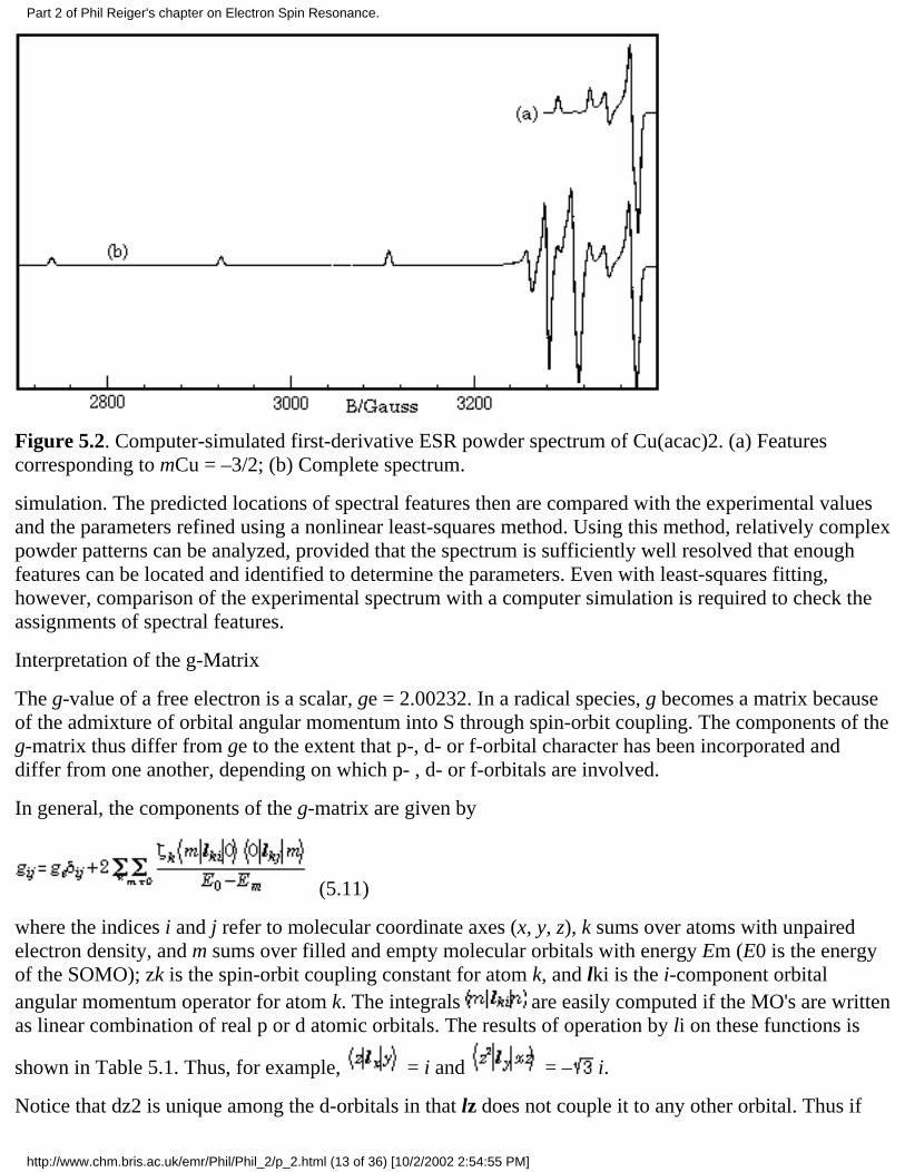
Powder spectra with hyperfine structure often can be interpreted similarly with spectral featuresidentified with orientation of the magnetic field along one of the g- and hyperfine matrix principal axes.However, this simple situation often breaks down. Using a first-order theory and one hyperfine coupling,Ovchinnikov and Konstantinov [36] have shown that eqs (5.10) may have up to six solutionscorresponding to observable spectral features. Three of these correspond to orientation of B alongprincipal axes, but the "extra lines" correspond to less obvious orientations. Even more extra lines maycreep in when the spin Hamiltonian is treated to second order or when there is more than one hyperfinecoupling. The problem is illustrated by the resonant field vs. cos q and f surface shown in Figure 5.1,corresponding to the mCu = –3/2 "line" in the spectrum of Cu(acac)2 (g = 2.0527, 2.0570, 2.2514; ACu =27.0, 19.5, 193.4 ¥ 10–4 cm–1) [36]. The minimum resonant field, B = 3290.7 G, corresponds to B alongthe z-axis (cos q = ±1). With B along the x-axis (cos q = 0, f = 0°), the surface shows a saddle point at3344.3 G, and with B along the y-axis (cos q = 0, f = 90°), there is a local minimum at 3325.5 G. Inaddition, another saddle point occurs in the yz-plane at B = 3371.2 G (cos q = ±0.482, f = 90°); the onlymaximum is in the xz-plane at B = 3379.0 G (cos q = ± 0.459, , f = 0°). Thus five features are expectedand indeed are shown in the computer-simulated spectrum of Cu(acac)2 shown in Figure 5.2. The twohigh-field features correspond to off-axis field orientations and thus are "extra lines". The situation ismore complex when the g- and hyperfine matrix principal axes are noncoincident (see below); in thiscase, none of the features need correspond to orientation of B along a principal axis direction.

Figure 5.1.Res-onant field asa function of cosq and f for themCu = -3/2 "line"of the frozensolution spectrumof Cu(acac)2; ESRparameters fromreference 36.



Since the analytical approach is so complicated, powder patterns have usually been analyzed bycomparing the experimental spectrum with a spectrum, computer-simulated using estimates of the g- andhyperfine matrix components. Parameters are then adjusted and another simulation computed until the fitis satisfactory (or the experimentalist loses patience with the problem). The most straightforwardcomputer simulation method [37] involves computation of the resonant magnetic field using eq (5.2) forca. 105 values of cos q and f for each set of nuclear spin quantum numbers. The field is then divided intoequal increments and the number of times the resonant field falls between Bi and Bi+1 is plotted vs. B togive an approximation to the unbroadened absorption spectrum. The absorption spectrum is thenbroadened by numerical convolution with a line shape function and differentiated to give the desiredsimulation. Although the "cut and try" approach to spectrum analysis works reasonably well when thereare small numbers of parameters, analysis of a complex spectrum is exceedingly tedious.

DeGray and Rieger [38] have developed a computer algorithm to locate powder pattern features inspectra, given estimates of the spin Hamiltonian parameters. The method employs a search of theresonant field surface in cos q, f space for maxima, minima, and saddle points. Since the searchprocedure requires computation of B for ~100 orientation, the method is much faster than a complete



Figure 5.2. Computer-simulated first-derivative ESR powder spectrum of Cu(acac)2. (a) Featurescorresponding to mCu = –3/2; (b) Complete spectrum.

simulation. The predicted locations of spectral features then are compared with the experimental valuesand the parameters refined using a nonlinear least-squares method. Using this method, relatively complexpowder patterns can be analyzed, provided that the spectrum is sufficiently well resolved that enoughfeatures can be located and identified to determine the parameters. Even with least-squares fitting,however, comparison of the experimental spectrum with a computer simulation is required to check theassignments of spectral features.

Interpretation of the g-Matrix

The g-value of a free electron is a scalar, ge = 2.00232. In a radical species, g becomes a matrix becauseof the admixture of orbital angular momentum into S through spin-orbit coupling. The components of theg-matrix thus differ from ge to the extent that p-, d- or f-orbital character has been incorporated anddiffer from one another, depending on which p- , d- or f-orbitals are involved.

In general, the components of the g-matrix are given by

(5.11)

where the indices i and j refer to molecular coordinate axes (x, y, z), k sums over atoms with unpairedelectron density, and m sums over filled and empty molecular orbitals with energy Em (E0 is the energyof the SOMO); zk is the spin-orbit coupling constant for atom k, and lki is the i-component orbitalangular momentum operator for atom k. The integrals are easily computed if the MO's are writtenas linear combination of real p or d atomic orbitals. The results of operation by li on these functions is

shown in Table 5.1. Thus, for example, = i and = – i.

Notice that dz2 is unique among the d-orbitals in that lz does not couple it to any other orbital. Thus if



the major metal contribution to the SOMO is dz2, gz will be close to the free electron value.Accordingly, when one g-matrix component is found close to the free electron value, it is often taken asevidence for a dz2-based SOMO; such reasoning should be applied with caution, however, sincecancellation of negative and positive terms in eq (5.11) could have the same effect.

Spin-orbit coupling to empty MO's (E0 – Em < 0) gives a negative contribution to gij whereas couplingto filled MO's has the opposite effect. Thus ESR spectra of d1 vanadium(IV) complexes generally haveg-values less than ge (admixture of empty MO's) whereas d9 copper(II) complexes have g-values greaterthan ge (admixture of filled MO's).

Since the g-matrix has only three principal values and there are almost always many potentiallyinteracting molecular orbitals, there is rarely sufficient information to interpret a g-matrix with completeconfidence. When a well resolved and reliably assigned optical spectrum is available, the energydifferences, E0 – Em, are known and can be used in eq (5.11). Extended Hückel MO calculations can beuseful (but don't trust EHMO energies!), but one is most commonly reduced to arguments designed toshow that the observed g-matrix is consistent with the interpretation placed on the hyperfine matrix.

Table 5.1. Angular momentum operations on the real p and d orbitals.

lx ly lz

0 –i i

i 0 –i

–i i 0

–i –i 2i

i –i –2i

i + i i –i

–i i – i i

– i i 0

Interpretation of the Hyperfine Matrix

Electron-nuclear hyperfine coupling arises mainly through two mechanisms:

The Fermi contact interaction between the nuclear spin and s-electron spin density; thiscontribution is isotropic and has been discussed above.

1.

The electron spin-nuclear spin magnetic dipolar interaction; this contribution is almost entirelyanisotropic, i.e., neglecting spin-orbit coupling, the average dipolar contribution to the hyperfinecoupling is zero.

2.



The general form of the dipolar contribution to the hyperfine term of the Hamiltonian is

(5.12)

where ge and gN are the electron and nuclear g-values, mB and mN are the Bohr and nuclear magnetons,and the matrix element is evaluated by integration over the spatial coordinates, leaving the spins asoperators. Equation (5.12) can then be written

(5.13)

where Ad is the dipolar contribution to the hyperfine matrix,

A = ·AÒ E + Ad (5.14)

(E is the unit matrix). In evaluating the matrix element of eq (5.12), the integration over the angularvariables is quite straightforward. The integral over r, however, requires a good atomic orbitalwavefunction. Ordinarily, the integral is combined with the constants as a parameter

(5.15)

P has been computed using Hartree-Fock atomic orbital wavefunctions and can be found in severalpublished tabulations [39-42]. Because of the dependence of P, dipolar coupling of a nuclear spinwith electron spin density on another atom is usually negligible.

If an atom contributes px, py, and pz atomic orbitals to the SOMO

(5.16)

the total p-orbital spin density is (in the Hückel approximation, i.e., neglecting overlap):

rp = cx2 + cy2 + cz2 (5.17)

and the dipolar contribution to the hyperfine matrix can be written

(Ad)ij = (2/5)Plij (5.18)

where the lij are lxx = 2cx2 – cy2 – cz2 (5.19a)

lyy = –cx2 + 2cy2 – cz2 (5.19b)

lzz = –cx2 – cy2 + 2cz2 (5.19c)

lij = –3cicj (i j) (5.19d)

The dipolar hyperfine matrix for p-orbitals can always be written



(5.20)

The p-orbital axis corresponds to the positive principal value of the matrix. When the p-orbitals arewritten as hybrids, the orbital shape is unchanged, but the principal axes of the hyperfine matrix, whichreflect the spatial orientation of the hybrid p-orbital, differ from those in which the SOMO wasformulated. Thus, for example, a p-hybrid with cx = cz (cy = 0) corresponds to a p-orbital with the majoraxis in the xz-plane and halfway between the x- and z-axes (Euler angle b = 45°).

Similarly, if an atom contributes d atomic orbitals to the SOMO,

(5.21)

the total d-orbital spin density is (in the Hückel approximation):

(5.22)

and the dipolar contribution to the hyperfine matrix is [43]

(Ad)ij = (2/7)Plij (5.23)

where P is given by eq (5.15) and the lij are:

(5.24a)

(5.24b)

(5.24c)

(5.24d)

(5.24e)

(5.24f)

The dipolar contribution to the hyperfine matrix for a pure d-orbital is

(5.25)

where the positive sign applies for dz2 and the lower sign to the other four orbitals. Hybrid combinationsof dyz, dxz, and dxy or dx2–y2 and dxy give a d-orbital of the same shape and the same dipolar matrix,



though the principal axes in general are different from the axes in which the SOMO was formulated.Other hybrid orbitals are generally of different shape, reflected by different principal values of thedipolar matrix, usually with different principal axes.

Spin-orbit coupling perturbs these results, adding terms to the diagonal matrix components on the orderof P(gi – ge). These can be neglected only when the g-matrix anisotropy is small. Calculation of thespin-orbit coupling corrections is fairly straightforward for mononuclear complexes where the SOMO iscomposed mainly of d-orbitals from a single metal [6,44,45]. In radicals with two or more transitionmetals, the spin-orbit coupling calculation is seriously nontrivial. A major part of the problem is that thesolution must be gauge-invariant, that is, it must not depend on the choice of coordinate system. Thisproblem was addressed in the context of spin-orbit coupling corrections to the g-matrix [46], with eq(5.11) as the result, but it has received only cursory examination with regard to spin-orbit contributions tohyperfine matrices [47]. Fortunately, polynuclear radicals containing first-row transition metals generallyhave g-matrix components sufficiently close to ge that the problem can be ignored. For organometallicradicals with second- and third-row transition metals, the problem is urgent; it is to be hoped that sometheoretician will deem the problem worthy of attention.

The AO composition of the SOMO can often be deduced from the dipolar hyperfine matrix, particularlywhen the radical has enough symmetry to restrict possible hybridization. Thus an axial hyperfine matrixcan usually be interpreted in terms of coupling to a single p- or d-orbital. A departure from axialsymmetry may be due to spin-orbit coupling effects, if (for example) A||= Az and Ax - Ay ª P(gx – gy). Ifthe departure from axial symmetry is larger, it is usually caused by d-orbital hybridization. Theprocedure is best illustrated by example.

Example–A low-spin Manganese(II) Complex

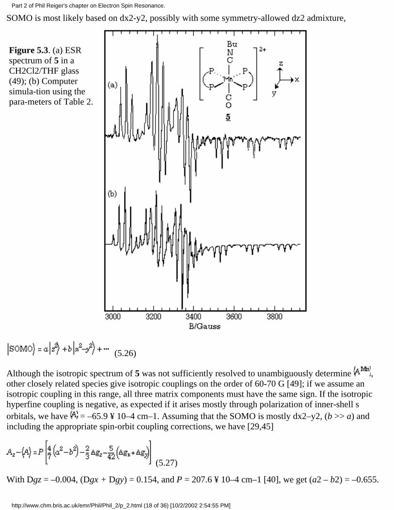
The spectrum of the low-spin manganese(II) complex, [Mn(dppe)2(CO)(CNBu)]2+, 5 (dppe =Ph2PCH2CH2PPh2) [48], in a CH2Cl2/THF glass is shown in Figure 5.3a. The spin Hamiltonianparameters, obtained from a least-squares fit of the field positions of the spectral features [49], are givenin Table 2, and a computer simulation based on those parameters is shown in Figure 5.3b.

Table 2. ESR Parameters for [Mn(dppe)2(CO)(CNBu)]2+.

g AMn/10-4 cm-1 AP/10-4 cm-1

2.107 30.2 27.2

2.051 20.6 25.3

1.998 146.9 26.4

5 has approximate C2v symmetry, although the actual symmetry is reduced to C2 or Cs, depending onthe conformation of the ethylene bridges of the dppe ligands. Since 5 has a nominal d5 configuration, theSOMO is expected to be one of the "t2g" orbitals of an idealized octahedral complex–dxz (b1), dyz (b2),or dx2-y2 (a1), where the representations refer to C2v. The energies of the dxz and dyz orbitals areexpected to be lowered by back-donation into the ¹* orbitals of the CO and CNBu ligands so that the



SOMO is most likely based on dx2-y2, possibly with some symmetry-allowed dz2 admixture,

Figure 5.3. (a) ESRspectrum of 5 in aCH2Cl2/THF glass(49); (b) Computersimula-tion using thepara-meters of Table 2.

(5.26)

Although the isotropic spectrum of 5 was not sufficiently resolved to unambiguously determine ,other closely related species give isotropic couplings on the order of 60-70 G [49]; if we assume anisotropic coupling in this range, all three matrix components must have the same sign. If the isotropichyperfine coupling is negative, as expected if it arises mostly through polarization of inner-shell sorbitals, we have = –65.9 ¥ 10–4 cm–1. Assuming that the SOMO is mostly dx2–y2, (b >> a) andincluding the appropriate spin-orbit coupling corrections, we have [29,45]

(5.27)

With Dgz = –0.004, (Dgx + Dgy) = 0.154, and P = 207.6 ¥ 10–4 cm–1 [40], we get (a2 – b2) = –0.655.



The departure from axial symmetry is due to spin-orbit coupling and/or dx2-y2/dz2 hybridization,

(5.28)

Substituting the parameters, we have ab = ±0.058. (The upper sign applies if the components are listed inthe order x, y, z in Table 2, the lower sign if the order is y, x, z) Finally, we get b2 = 0.660, a2 = 0.005.The dz2 component is not really significant, given the accuracy of the data and the theory, i.e., most ofthe departure from axial symmetry can be explained by the spin-orbit coupling correction.

Using eq (5.11), the g-matrix components are found to be

(5.29a)

(5.29b)

(5.29c)

If we assume coupling with single pure dyz, dxz, and dxy orbitals, we have DEyz = 16z, DExz = 19z,DExy = –1100z, qualitatively consistent with the expected MO energy level scheme.

Example: Some Cobalt(0) Radical Anions

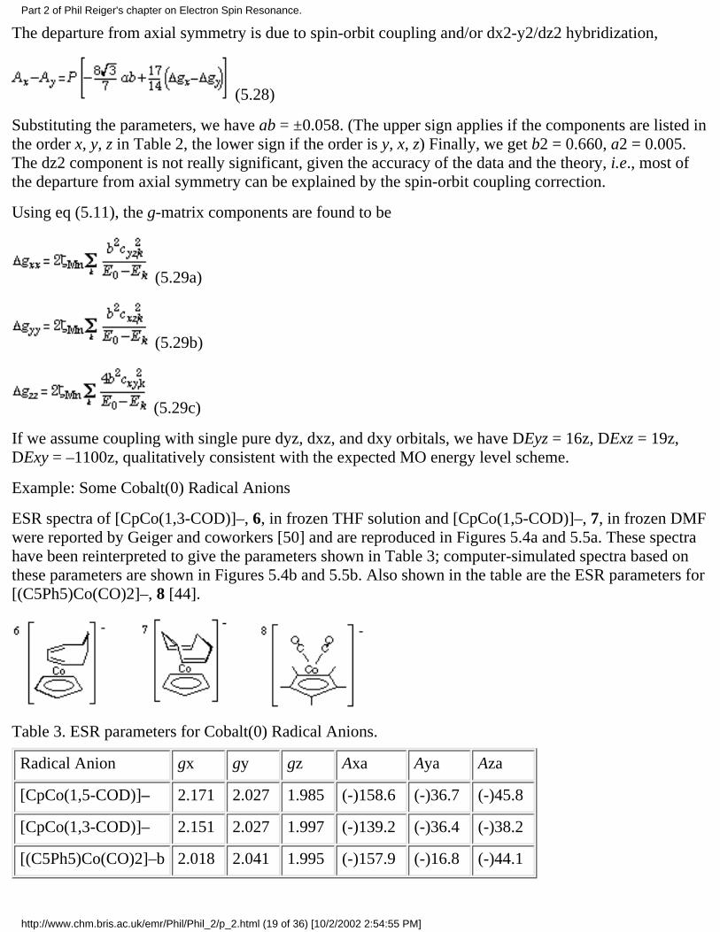
ESR spectra of [CpCo(1,3-COD)]–, 6, in frozen THF solution and [CpCo(1,5-COD)]–, 7, in frozen DMFwere reported by Geiger and coworkers [50] and are reproduced in Figures 5.4a and 5.5a. These spectrahave been reinterpreted to give the parameters shown in Table 3; computer-simulated spectra based onthese parameters are shown in Figures 5.4b and 5.5b. Also shown in the table are the ESR parameters for[(C5Ph5)Co(CO)2]–, 8 [44].

Table 3. ESR parameters for Cobalt(0) Radical Anions.

Radical Anion gx gy gz Axa Aya Aza

[CpCo(1,5-COD)]– 2.171 2.027 1.985 (-)158.6 (-)36.7 (-)45.8

[CpCo(1,3-COD)]– 2.151 2.027 1.997 (-)139.2 (-)36.4 (-)38.2

[(C5Ph5)Co(CO)2]–b 2.018 2.041 1.995 (-)157.9 (-)16.8 (-)44.1



a Units of 10–4 cm–1. b From reference 44.

The hyperfine matrix components musthave identical signs in order that theaverage values match the observedisotropic couplings; we assume thesigns are negative since the isotropiccouplings almost certainly arise frompolarization of inner shell s orbitals (seebelow).

The SOMO in these radicals is expectedfrom extended Hückel MO calculations[50,51] to be primarily cobalt 3dyz incharacter. In the Cs symmetry of theradicals, dyz belongs to the a"representation and d-hybridization ispossible only with dxy. Assuming thatsuch hybridization is negligible, theg-matrix components are given by [44]

(5.30a)

(5.30b)

(5.30c)

The dipolar contribution to thehyperfine matrix is given by eq (5.20),but spin-orbit coupling contributionsare significant. These often can be ex-

Figure 5.4. ESR spectrum of[CpCo(1,3-COD)]–; (a) experimentalspectrum in frozen THF solution (fromreference 50); (b) computer-simulation,based on the parameters of Table 3.

pressed in terms of the g-matrix components (as in the Mn(II) example discussed above), but herespin-orbit coupling with the four other d-orbitals contributes somewhat differently to the g-matrix and tothe hyperfine matrix. The simplest way of expressing the hyperfine matrix is in terms of the isotropiccoupling, the x-component, and the departure from axial symmetry,



(5.31a)

(5.31b)

(5.31c)

With the assumed signs of the hyperfine components of Table 3, eq (5.31b) can be used unambiguouslyto compute a2 = rd with the results shown in Table 4.

Since 3dyz/4s admixture is symmetry-forbidden for these radicals, the Fermi contact contribution to theisotropic coupling must be entirely from spin polarization,

As = Qdrd (5.32)

Thus we can obtain an independent estimate of the d-electron spin density from the values of As, takingQd = –131 ¥ 10–4 cm–1, estimated from the isotropic cobalt coupling in [PhCCo3(CO)9]–. The resultsare shown in the last column of Table 4. The spin densities estimated from the isotropic couplings areconsistently about 10% higher than those from the dipolar coupling matrix, suggesting a systematic errorin one of the parameters, but a reliable ordering of the spin densities.

Table 4. d-Electron spin densities in cobalt(0) radical anions.

Radical Anion rd Asa As/Qd

[CpCo(1,5-COD)]- 0.681 -97.0 0.740

[CpCo(1,3-COD)]- 0.591 -87.2 0.666

[(C5Ph5)Co(CO)2]-b 0.540 -77.4 0.591

a in units of 10–4 cm–1.

The g-matrix presents an interesting problem in these cases. EHMO calculations [50,51] suggest that theSOMO is the highest-energy MO which is primarily cobalt 3d in character. At lower energy is an orbitalwith dxz character and still lower, but grouped at about the same energy, are MO's with dx2–y2, dxy, anddz2 contributions. Equations (5.30) then would suggest that Dgxx/4 Å Dgyy < Dgzz. With theassignments of Table 4, the first relationship is approximately correct for 6 and 7, but very poor for 8.The second relationship is not found for any of the anions. Reversing the y and z assignments makes theagreement worse. In discussing this problem for 8 [44], we postulated admixture of some cobalt 4pycharacter in the SOMO,



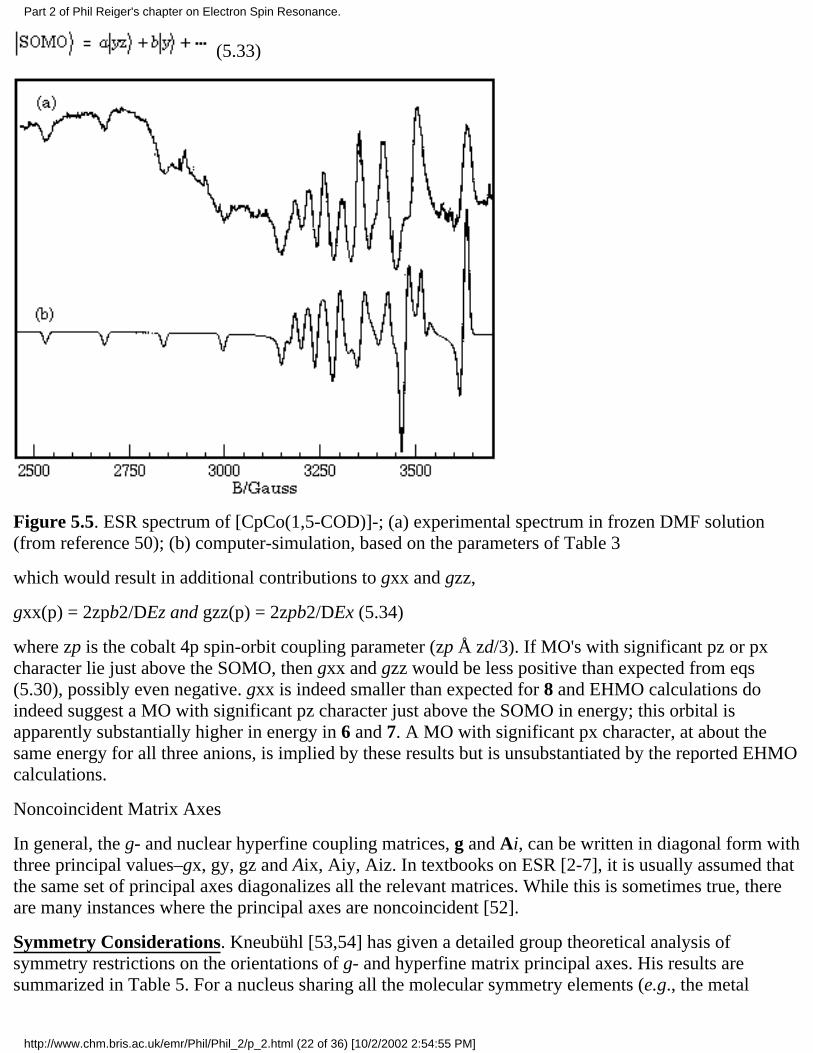
(5.33)

Figure 5.5. ESR spectrum of [CpCo(1,5-COD)]-; (a) experimental spectrum in frozen DMF solution(from reference 50); (b) computer-simulation, based on the parameters of Table 3

which would result in additional contributions to gxx and gzz,

gxx(p) = 2zpb2/DEz and gzz(p) = 2zpb2/DEx (5.34)

where zp is the cobalt 4p spin-orbit coupling parameter (zp Å zd/3). If MO's with significant pz or pxcharacter lie just above the SOMO, then gxx and gzz would be less positive than expected from eqs(5.30), possibly even negative. gxx is indeed smaller than expected for 8 and EHMO calculations doindeed suggest a MO with significant pz character just above the SOMO in energy; this orbital isapparently substantially higher in energy in 6 and 7. A MO with significant px character, at about thesame energy for all three anions, is implied by these results but is unsubstantiated by the reported EHMOcalculations.

Noncoincident Matrix Axes

In general, the g- and nuclear hyperfine coupling matrices, g and Ai, can be written in diagonal form withthree principal values–gx, gy, gz and Aix, Aiy, Aiz. In textbooks on ESR [2-7], it is usually assumed thatthe same set of principal axes diagonalizes all the relevant matrices. While this is sometimes true, thereare many instances where the principal axes are noncoincident [52].

Symmetry Considerations. Kneubühl [53,54] has given a detailed group theoretical analysis ofsymmetry restrictions on the orientations of g- and hyperfine matrix principal axes. His results aresummarized in Table 5. For a nucleus sharing all the molecular symmetry elements (e.g., the metal



nucleus in a mononuclear complex), the hyperfine matrix is subject to the same restrictions as theg-matrix. In orthorhombic or axial symmetry, such nuclear hyperfine matrices necessarily share principalaxes with the g-matrix. In monoclinic symmetry, one hyperfine axis is also a g-matrix axis, but the othertwo may be different. In triclinic symmetry (C1 or Ci), none of the three principal axes need be sharedby the g-matrix and hyperfine matrix. The hyperfine matrix for a ligand atom (or for a metal inpolynuclear complexes) is constrained only by the symmetry elements which the nucleus shares with themolecule.

Table 5. Symmetry restrictions on g-matrix components.

Symmetry

Point Groups

Restrictionson DiagonalElements

Restrictions onOff-DiagonalElements

RequiredMatrixAxes

Triclinic C1,Ci none none none

Monoclinic C2,Cs,C2h none gxz = gyz = 0 z

Orthorhombic C2v,D2,D2h none gxz = gyz = gxy=0

x,y,z

Axial Cn,Cnv,Cnh,Dn,Dnd,Dnh, n >2

gxx = gyy gxz = gyz = gxy=0

x,y,z

Although symmetry considerations often permit g- and hyperfine matrix principal axes to benoncoincident, there are relatively few cases of such noncoincidence reported in the literature. Most ofthe examples discussed by Pilbrow and Lowrey in their 1980 review [52] are cases of transition metalions doped into a host lattice at sites of low symmetry. This is not to say that matrix axis noncoincidenceis rare but that the effects have only rarely been recognized.

Experimental Determination of Matrix Axis Orientations. We have seen that spectra of dilute singlecrystals are analyzed in a way that gives the orientations of the g- and hyperfine matrix principal axesrelative to the crystal axes. Historically, most of the information on noncoincident matrix axes is derivedfrom such studies.

At first glance, it would appear that all orientation dependence should be lost in the spectrum of arandomly oriented sample and that location of the g- and hyperfine matrix principal axes would beimpossible. While it is true that there is no way of obtaining matrix axes relative to molecular axes froma powder pattern, it is frequently possible to find the orientation of a set of matrix axes relative to thoseof another matrix.

The observable effects of matrix axis noncoincidence on powder patterns range from blatantly obvious tonegligible. In general, the effects of axis noncoincidence will be more noticeable if two (or more)matrices have large anisotropies which are comparable in magnitude, e.g., DgmBB Å DA. This followsfrom the fact that minimum and maximum resonant fields are determined by a competition between



extrema in the angle-dependent values of g and A. Consider the case of noncoincident g- and hyperfinematrix axes. For large values of |mI|, the field extrema will be determined largely by the extrema in theeffective hyperfine coupling and will occur at angles close to the hyperfine matrix axes, but for small|mI|, the extrema will be determined by extrema in the effective g-value and will correspond to anglesclose to the g-matrix axes. The result of such a competition is that a series of features which would beequally spaced (to first order) acquires markedly uneven spacings.

There are two corollaries stemming from this generalization. Since spin 1/2 nuclei give only twohyperfine lines, there can be no variation in spacings. Thus powder spectra cannot be analyzed to extractthe orientations of hyperfine matrix axes for such important nuclei as 1H, 13C, 19F, 31P, 57Fe, and103Rh. Secondly, since the observable effects in powder spectra depend on the magnitude of the matrixanisotropies, the principal axes of the hyperfine matrix for a nucleus with small hyperfine couplinggenerally cannot be located from a powder spectrum, even though the relative anisotropy may be large.

Example–Chromium Nitrosyl Complex

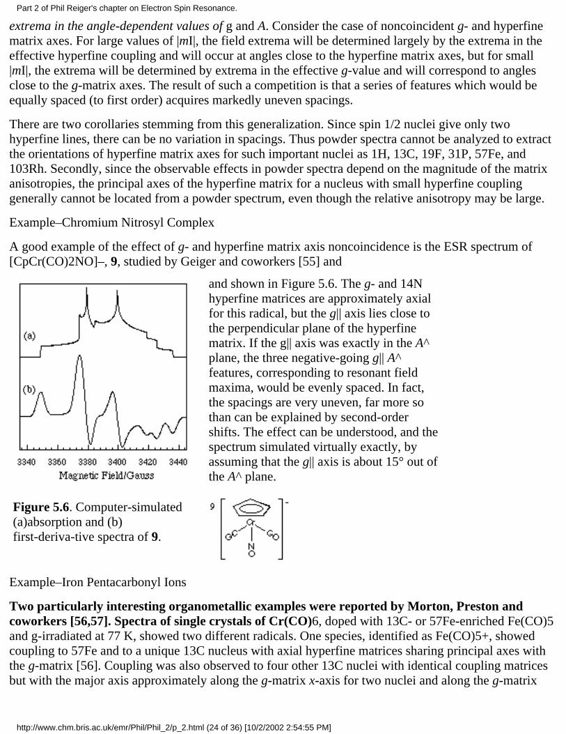
A good example of the effect of g- and hyperfine matrix axis noncoincidence is the ESR spectrum of[CpCr(CO)2NO]–, 9, studied by Geiger and coworkers [55] and

Figure 5.6. Computer-simulated(a)absorption and (b)first-deriva-tive spectra of 9.

and shown in Figure 5.6. The g- and 14Nhyperfine matrices are approximately axialfor this radical, but the g|| axis lies close tothe perpendicular plane of the hyperfinematrix. If the g|| axis was exactly in the A^plane, the three negative-going g|| A^features, corresponding to resonant fieldmaxima, would be evenly spaced. In fact,the spacings are very uneven, far more sothan can be explained by second-ordershifts. The effect can be understood, and thespectrum simulated virtually exactly, byassuming that the g|| axis is about 15° out ofthe A^ plane.

Example–Iron Pentacarbonyl Ions

Two particularly interesting organometallic examples were reported by Morton, Preston andcoworkers [56,57]. Spectra of single crystals of Cr(CO)6, doped with 13C- or 57Fe-enriched Fe(CO)5and g-irradiated at 77 K, showed two different radicals. One species, identified as Fe(CO)5+, showedcoupling to 57Fe and to a unique 13C nucleus with axial hyperfine matrices sharing principal axes withthe g-matrix [56]. Coupling was also observed to four other 13C nuclei with identical coupling matricesbut with the major axis approximately along the g-matrix x-axis for two nuclei and along the g-matrix



y-axis for the other two. The parameters are listed in Table 6. If the radical is square pyramidal (C4v)Fe(CO)5+, 10, the principal axes of the g-matrix must be the molecular axes (the C4 axis and normals tothe reflection planes). The iron atom and the carbon of the axial CO group have the full symmetry of thegroup and so these hyperfine matrices must share principal axes with the g-matrix. The four equatorialcarbonyl carbons, on the other hand, lie in reflection planes, but not on the C4-axis and so aresymmetry-required to share only one principal axis with the g-matrix. In fact, the major matrix axes forthe equatorial carbons are tilted slightly in the -z direction from the ideal locations along the ±x and ±yaxes. The g-matrix suggests that the metal contribution is dz2 and the iron hyperfine matrix then can beused to estimate about 55% iron 3d and 34% axial carbon 2pz spin density. The spin density on theequatorial carbons then is mostly negative and due to spin polarization.

Table 6. ESR Parameters for Fe(CO)5+ and Fe(CO)5–.a

Fe(CO)5+: g|| = 2.001 A||Fe = (+)9.4 A||C1 =(+)19.6

A||C2-C5 =(+)6.4

g^ = 2.081 A^Fe = (-)6.2 A^C1 = (-)17.6 A^C2-C5 =(+)8.6

Fe(CO)5–: g1 = 1.989 A1Fe = (+)6.7 A1C1 =(+)87.4

g2 = 2.003 A2Fe = (-)4.5 A2C1 =(+)70.7

g3 = 2.010 A3Fe = (-)3.2 A3C1 =(+)65.7

a Coupling constants in units of 10–4 cm–1. Data from references 56 and 57.

The other species observed in irradiated Fe(CO)5-doped crystals of Cr(CO)6 also showed coupling to57Fe, to a unique 13C, and to four other carbons. However, in this case g, AFe, and AC1 have only onematrix axis in common (that corresponding to the third component of each matrix listed in Table 6). Theother 57Fe hyperfine axes are rotated by about 27° and those of the 13C hyperfine matrix by about 48°relative to the g-matrix axes. Insufficient data were accumulated to determine the complete hyperfinematrices for the other four carbons, but the components are considerably smaller (4 - 15 ¥ 10–4 cm–1).The hyperfine matrices suggest about 38% iron 3dz2, 18% carbon 2p, and 6% carbon 2s spin densities.Using detailed arguments regarding the orientation of the g-matrix axes relative to the crystal axes, the



authors conclude that the carbon 2p axis is oriented at about 106° relative to the Fe-C bond axis and thatthe Fe-C-O bond angle is about 119°.

The most striking feature of these results is the orientation of the unique 13C hyperfine matrix axes,relative to those of the 57Fe hyperfine axes. This orientation led Fairhurst, et al.[57], to assign thespectrum to Fe(CO)5–, 11, and to describe the species as a substituted acyl radical. However, theseauthors did not discuss the orientation of the g-matrix axes. The y-axis, normal to the reflection plane, iscommon to all three matrices. The x- and z- axes of the g-matrix, on the other hand are oriented about 27°away from the corresponding 57Fe hyperfine matrix axes. Since the iron d-orbital contribution to theSOMO appears to be nearly pure dz2, the 57Fe hyperfine matrix major axis must correspond to the localz-axis, assumed to be essentially the Fe-C bond. Thus we must ask: Why are the g-matrix axes different?The SOMO can be written

(5.35)

where a = 0.62, bx = -0.41, and bz = 0.12. Spin-orbit coupling will mix the SOMO with MO's havingiron dyz or dxz character, but dyz is involved in the p orbitals of the C=O group,

(5.36)

Assuming that there is only one p orbital close enough in energy to couple significantly, eq (5.11) givesthe g-matrix components:

(5.37a)

(5.37b)

Dgzz = 0 (5.37c)

(5.37d)

The g-matrix can be diagonalized by rotation about the y-axis by the angle b,

(5.38)

With b = 27°, this expression gives cyz/cy Å 0.5, a reasonable result.

This may be a rather general effect; if the unpaired electron in a radical is delocalized asymmetrically,and other MO's are similarly delocalized, the g-matrix will have off-diagonal elements which may belarge enough to shift the principal axes away from the molecular coordinate system.



Example–Another low-spin Manganese(II) Complex

The low-spin manganese(II) complex, [Mn(dppe)2(CO)(CNBu)]2+, 5, gave us a textbook example of awell-behaved ESR spectrum characterized by coincident g- and hyperfine matrix principal axes. Thenearly identical complex, [Mn(dppm)2(CO)(CN)]+, 12+, provides us with a good example ofnon-coincident principal axes. The frozen solution spectrum, shown in Figure 5.7, shows that

Figure 5.7. ESR spectrum of 12+ inCH2Cl2/C2H4Cl2 at 90 K; fromreference (49).

the "parallel" features are not evenlyspaced. The spectrum can beunderstood if the z-axes of the g- andA-matrices are displaced by b = 19.6°.This, of course, tells us that themolecule does not have C2vsymmetry, and that, unlike the dppeanalog, dx2-y2 is not the only Mncontribution to the SOMO. One wayof interpreting the results is that theMn contribution to the SOMOincorporates a small amount of dxzcharacter. The consequence of thishybridization would be to tilt the "x"lobes of dx2-y2 up and down, i.e.,rotation about the y-axis. The reasonfor this hybridization is not difficult todiscover. If the CH2 groups of thedppm ligands were coplanar with Mn,the "x" lobes of the dx2-y2 SOMOwould be directed toward the carbonatoms and an anti-bonding

interaction would result. In order toavoid this interaction, two thingshappen: (1) incorporation of dxzchar-acter tilts the lobes up and down,away from the C atoms. At the sametime, the x-ray structure of the Mn(II)cation shows (Figure 5.8) that the CH2groups tilt down and up, furtherdecreasing the anti-bonding interaction.With only one electron in the SOMO,the anti-bonding interaction is strongenough to produce this distortion. Withtwo electrons, the neutral parent Mn(I)complex would be expected to be evenmore distorted, and an x-ray structureshows that the up and downdisplacements of the CH2 groups is

Figure 5.8. X-ray structure of 12+,showing methylene groups tilted up anddown to avoid anti-bonding interactionwith dx2-y2 SOMO.



approximately doubled.

Example–Chromium(I) Piano-Stool Complex

Ordinarily, there is no way of extracting the orientation of the principal axes of the g-matrix from apowder or frozen solution ESR spectrum. However, there are exceptional circumstances in which natureis kind to the experimentalist!

Spectra of the low-spin d5 Cr(I)complex, [(C5Ph5)Cr(CO)2PMe3] 13(58), are shown at 125 and 200 K inFigure 5.9 The low-temperaturespectrum shows three sets of doublets,corresponding to the threeg-components (2.104, 2.013, 1.994),each a doublet due to hyperfinecoupling to 31P. At 200 K, above thefreezing point of toluene, the spectrumstill appears as a "powder pattern", butthe "perpendicular" features are nearlyaveraged and the "parallel" featureshave shifted upfield (g|| = 2.090, g^ =2.012). The exceptionally bulky C5Ph5ligand apparently moves very slowly at200 K but on the ESR time scale theCr(CO)2PMe3 moiety rotates quickly,producing a spectrum averaged aboutthe Cr-C5 axis. With this interpretation,we can assign this axis as the principalaxis for g|| measured at 200 K and,assuming that the g|| axis differs fromthe gz axis by

Figure 5.9. Spectra of 13 in toluene at125 and 200 K; from reference (58).

the angle b and that gz and gx are averaged according to

2g||2 = gz2 + gx2 + (gz2 + gx2) cos22b

Substitution of the g-components gives b = 15°

The symmetry of the complex is at most Cs, requiring one of the g-matrix principal axes to be normal tothe plane of symmetry, assumed to be xz. ¹-back-bonding to the CO ligands is expected to lead to ahybrid SOMO. If, as suggested by extended Hückel MO calculations, the SOMO and first HOMO are ofa' symmetry, and the second HOMO of a" symmetry:



the g-matrix components can be computed:

Rotation about the y-axis by b diagonalizes the matrix, and we find

The single experimental observable, b, is hardly enough to evaluate the LCAO coefficients for theSOMO and second HOMO, but we can compare the results of an extended Hückel MO calculation.(Since zCo and E0 – E2 cancel in the calculation of tan 2b, the EHMO calculation could come close).The results are: a1 = 0.538, a2 = 0.216, a3 = –0.194, c1 = 0.582, c2 = –0.061, b = 14.8°. If we were tosubstitute these LCAO coefficients, together with the EHMO energy difference, into the expressions forgxx, gyy, gzz, and gxz, the results would be in very poor agreement with experiment; the moral here isthat EHMO calculations, lacking charge self-consistency, usually have large errors in the energies, butthe MO wavefunctions are often fairly accurate.

Example–[(RCCR')Co2(CO)6]- and [SFeCo2(CO)9]-

Noncoincident matrix axis effects are seen in the frozen solution spectra of [(RCCR')Co2(CO)6]–, 14[59], and [SFeCo2(CO)9]–, 15 [60], but the effects are rather more subtle than those discussed above.

In these cases, the g-matrix is nearly isotropic, but the principal axes of the two 59Co hyperfine matricesare noncoincident. The largest hyperfine matrix component (ay = 66.0 G in the case of 15) results in 15features, evenly spaced (apart from small second-order shifts). Another series of features, less widelyspaced, shows some variation in spacing and, in a few cases, resolution into components. This behaviorcan be understood as follows: Suppose that the hyperfine matrix y-axes are coincident and considermolecular orientations with the magnetic field in the xz-plane. To first order, the resonant field then is

B = B0 - m1a+ - m2a- (5.39)



where B0 = hn/gmB and

a±2 = az2cos2(q ± b) + ax2sin2(q ± b) (5.40)

where b describes the orientation of the hyperfine matrix z-axes relative to the g-matrix z-axis. Since g isnearly isotropic, the extrema in B are determined mostly by the hyperfine term. When m1 = m2, a+ anda- are equally weighted and the extrema occur at q = 0 or 90°, but when m1 m2, the extrema correspondto other angles. Consider, for example, the five components of the m1+ m2 = +3 feature. With |az| = 53.6G, |ax| = 15.5 G, b = 18°, the hyperfine contributions to the field extrema and the corresponding values ofq are given in Table 7. In the experimental spectrum of 15, two resolved field maximum features wereseen, corresponding to the first two and the last three of the above components. Since the resolution issensitive to the noncoincidence, it was possible to fit the experimental spectrum to obtain b quiteaccurately.

Table 7. Splitting of M = 3 features in [SFeCo2(CO)9]– Spectrum.

(m1, m2) qmin (B-B0)min/G qmax (B-B0)max/G

+7/2,-1/2 -20° 37.0 +67° 166.1

-1/2,+7/2 +20° 37.0 -67° 166.1

+5/2,+1/2 -15° 55.3 +78° 156.9

+1/2,+5/2 +15° 55.3 -78° 156.9

+3/2,+3/2 0° 66.5 90° 153.6

It is relatively easy to understand the significance of the noncoincident matrix axes in these cases. For 14,the C2v molecular symmetry permits a specific prediction of the possible matrix axis orientations. Theg-matrix principal axes must be coincident with the molecular symmetry axes. The two cobalt nuclei arelocated in a reflection plane (which we label xz) so that symmetry requires the y-axis to be a principalaxis for all three matrices. The other two axes may be rotated, relative to the molecular x- and z-axes, by±b. (Since the two nuclei are symmetrically equivalent, the rotations must be equal and opposite.)

Since the magnitudes and probable signs of the cobalt hyperfine matrices suggest a SOMOpredominantly dz2 in character, the major axes of the hyperfine matrices approximate the local z-axes atthe cobalt atoms and the angular displacement indicates a bent Co-Co anti-bonding interaction, asshown in structure 16, where the C-C or Fe-S bond axis (the molecular y-axis) is perpendicular to theplane of the page. Comparison with the crystal structure of neutral (Ph2C2)Co2(CO)6 [61] shows thatthese local axes are roughly in the direction of the axial carbonyl ligands (the Co-CO bond is tilted 28°away from the Co-Co vector). Thus it seems reasonable to say that the local axes on a metal aredetermined primarily by the more strongly interacting ligands and that bonds to other atoms can bedescribed as bent.

Example–(o-xylylene)-Mn(dmpe)2



As part of a study of Mn(II) dialkyls, Wilkinson, Hursthouse, and coworkers [62] reported the ESRspectrum of the approximately octahedral (o-xylylene)Mn(dmpe)2, 17, Figure 5.10a (dmpe =Me2PCH2CH2PMe2). The spectrum was interpreted assuming coincident g- and hyperfine matrix axes,but a simulation based on the reported parameters gave a very poor fit to the published spectrum. Oncloser examination, it was realized that this is a rather

extreme example of a spectruminfluenced by noncoincident g- andhyperfine matrix principal axes. Theclue evident in the spectrum is thelarge gap between the mMn = –1/2and +1/2 "parallel" features,suggesting one or more extrafeatures. Figure 5.11 shows a set ofsimulated spectra for a hypotheticallow-spin Mn(II) species; all sevenspectra correspond to the same g-and hyperfine matrices, but the angleb, between the g- and hyperfinematrix z-axes, varies from 0 to 90°.As shown in Figure 5.11, it ispossible to obtain spectra with morethan six resolved "parallel" features.Indeed, the spectrum is sufficientlysensitive to the angle that b can beevaluated quite precisely. The finalparameters for 17, based onleast-squares fitting of the positionsof the resolved features and theisotropic parameters [53], are givenin Table 8; a computer simulationusing these parameters is shown inFigure 5.10b.

Figure 5.10. (a) ESR spectrum of(o-xylylene)Mn(dmpe)2 in frozen toluenesolution (from reference 53); (b) Computersimulation of spectrum using parameters ofTable 8.

Table 8. ESR Parameters for (o-xylylene)Mn(dmpe)2, 17.a

g AMn AP

2.110 27 24.5

2.035 27 24.5



2.000 125 24.5

a Hyperfine matrix components in units of 10-4 cm-1; b = 41°.

Figure 5.11.Computer-simulatedESR spectra for ahypothetical low-spinMn(II) radical with g =(2.100, 2.050, 2.000),AMn = (150, 25, 25) ¥10–4 cm–1, for variousvalues of b, the Eulerangle between theg-matrix and hyperfinematrix z-axes.

17 has approximate C2v symmetry, but the ethylene bridges of the dmpe ligands destroy the reflectionplanes; the x-ray structure [53] shows a small fold at the methylene groups of the o-xylylene ligandwhich destroys the C2 axis. Thus the molecule can be regarded, with increasing accuracy, as C2v, Cs,C2, or C1. In order to explain the matrix axis noncoincidence, the metal contribution to the SOMO mustbe a d-hybrid. Since 17 is a d5 low-spin Mn(II) species, the SOMO is expected to be dominated by oneof the orbitals of the octahedral t2g set–dxz, dyz, or dx2-y2. This is consistent with a clue contained inthe ESR parameters. The four 31P couplings are apparently equivalent, and all are relatively small. Thusno lobe of the SOMO can be directed toward a phosphorus atom, and major dxy or dz2 contributions tothe SOMO can be ruled out. Consider the twelve binary hybrids based on these orbitals which are listed



in Table 9. Since we know that the

Table 9. SOMO Candidates: Binary d-Hybrids.

NumberRepresentation

Major MinorApprox.Major Common

Cs C2 d-AO d-AO HF Axis Axis

1 a' a dx2-y2 dz2 z x,y,z

2 a' - dx2-y2 dyz z x

3 a' - dyz dx2-y2 x x

4 a' - dyz dz2 x x

5 a" - dxz dxy y x

6 - a dx2-y2 dxz z y

7 - a dxz dx2-y2 y y

8 - a dxz dz2 y y

9 - b dyz dxy x y

10 - - dx2-y2 dxy z z

11 - - dxz dyz y z

12 - - dyz dxz x z

hyperfine matrix major axis is not a g-matrix principal axis, we can immediately reject hybrids 1, 3, 4, 7,8, and 10 for which the major axis is a common axis. Hybrids 2 and 6, 5 and 9, and 11 and 12 differ onlyin the x- and y-labels and are essentially indistinguishable, so that there are only three cases to consider indetail.

Hybrid 6 can be written

(5.41)

Straightforward application of eqs (5.24) yields a hyperfine matrix which can be diagonalized by rotationabout the y-axis by the angle b,

tan 2b = –2b/a (5.42)

The g-matrix can be written in relatively simple form if we assume that the only MO's close enough inenergy to contribute significantly are the filled MO's, primarily dxz and dyz in character. With this



assumption, we obtain a matrix which can be diagonalized by rotation about the y-axis by b',

(5.43)

For reasonable values of the hybridization ratio, b/a up to about 0.5, b and b' can differ by only a fewdegrees and this kind of hybrid cannot explain the matrix axis noncoincidence. Following the samereasoning with x and y interchanged, exactly the same conclusions can be reached for hybrid 2.

Hybrids 11 and 12 are

(5.44)

In this case, the hyperfine matrix remains axial, independent of the hybridization ratio, although theprincipal axes are rotated in the xy-plane by an angle a equal to angle b of eq (5.43). Assuming that onlyMO's with predominantly dxz, dyz, or dx2–y2 character contribute, a g-matrix is found which can bediagonalized by rotation in the xy-plane by the angle a', also given by eq (5.43). Thus this hybrid givesidentical g- and hyperfine matrix principal axes for all hybridization ratios.

Finally, hybrid 9,

(5.45)

gives an axial hyperfine matrix with principal axes rotated in the xz-plane by an angle b, given by eq(5.43). The g-matrix is somewhat more complicated,

(5.46)

Diagonalization requires rotation about the y-axis by the angle b',

(5.47)

where

(5.48)



Since the energy differences, DEx2–y2 and DExz are expected to be comparable, the parameter Q isprobably not far from unity. For Q = 1, eq (5.47) has a particularly simple form, tan 2b' = +2a/b so that,for small b/a, we expect b Å 0 and b' Å 45°, entirely consistent with experiment. The axial hyperfinematrix is in agreement with experiment, and the principal values of the g-matrix can also be rationalizedwith reasonable values of Q and b/a. A small rotation of dyz about the y-axis might reflect the smalldisplacements of the phosphorus atoms from the idealized octahedral positions.

An extended Hückel MO calculation on 15 supports the assumptions made in the above analysis in thatthe three "t2g" orbitals are indeed close together in energy and remain nearly nonbonding metal-basedd-orbitals. The detailed agreement is less satisfactory: the SOMO is predicted to be primarily dx2–y2with a small dxz admixture (hybrid 6 of Table 9), a result which can be ruled out from our analysis of theESR results. The EHMO overlap matrix based on the x-ray structure suggests that the molecule is muchcloser to C2 symmetry than to Cs. If we accept that conclusion, then dxz/dxy hybridization is less likelythan dyz/dxy, as we tacitly assumed above.

We considered several alternative explanations for the matrix axis noncoincidence in 15. In particular, itseemed possible that delocalization of spin density into the o-xylylene ligand, either through the s-bondsor into the p-system, might lead to significant contributions to the off-diagonal terms of the g-matrix.While the EHMO calculations suggest that the MO's containing dx2–y2 and dyz do have contributionsfrom the carbon atoms of the o-xylylene group, the amount is far too small to rationalize rotation of theg-matrix axes by 41°; indeed, to explain the effect in this way would require each of several carbonatoms to contribute 5% or more to the MO's with dx2–y2 or dyz character, unreasonably largeconsidering the poor overlap of these metal d-orbitals with the relevant carbon orbitals.

6. Molecules with More than One Unpaired Electron

Molecules with two or more unpaired electrons may be divided into two classes: By far the mostcommon examples are molecules where the unpaired electrons are contained in a set of degenerateatomic or molecular orbitals with qualitatively similar spatial distributions, e.g., an octahedral Cr(III)(4A2g) or Ni(II) (3A2g) complex, or a triplet state molecule like O2, or the excited triplet states ofnaphthalene or benzophenone.

A second class of molecules withtwo unpaired electrons has the twoelectrons localized, to a firstapproximation, in different parts ofthe molecule. We refer to suchmolecules as biradicals. Examplesare the dinitroxides, and certainbinuclear vanadium(IV) andcopper(II) complexes.

From the point of view of ESR spectroscopy, the distinction between molecules with one unpairedelectron and those with more than one lies in the fact that electrons interact with one another; theseinteractions lead to additional terms in the spin Hamiltonian and additional features in the ESR spectrum.The most important electron-electron interaction is coulombic repulsion; with two unpaired electrons,repulsion leads to the singlet-triplet splitting. As we will see, this effect can be modelled by adding a



term, , to the spin Hamiltonian, where J is called the exchange coupling constant and turns out tobe equal to the singlet-triplet splitting.



References1 A. Hudson, Electron Spin Resonance, 1988,11A , 55-76.

2 P. B. Ayscough, Electron Spin Resonance in Chemistry, Methuen, London, 1967.

3 P. W. Atkins and M. C. R. Symons, The Structure of Inorganic Radicals, Elsevier, Amsterdam, 1967.

4 A. Abragam and B. Bleaney, Electron Paramagnetic Resonance of Transition Ions, Clarendon Press,Oxford, 1970.

5 J. E. Wertz and J. E. Bolton, Electron Spin Resonance, McGraw-Hill, New York, 1972.

6 N. M. Atherton, Electron Spin Resonance, Ellis Horwood, Chicester, 1973.

7 W. Gordy, Theory and Applications of Electron Spin Resonance, Wiley, New York, 1980.

8 J. R. Pilbrow, Transition Ion Electron Paramagnetic Resonance, Clarendon Press, Oxfor, 1990.

9 F. E. Mabbs and D. Collison, Electron Paramagnetic Resonance of d Transition Metal Compounds,Elsevier, Amsterdam, 1992.

10 G. Breit and I. I. Rabi, Phys. Rev. 1931, 38, 2082-2083.

11 S. I. Weissman, J. Townsend, G. E. Paul, and G. E. Pake, J. Chem. Phys. 1953, 21, 2227.

12 L. V. Casagrande, T. Chen, P. H. Rieger, B. H. Robinson, J. Simpson, and S. J. Visco, Inorg. Chem.1985, 23, 2019-2025.

13 B. M. Peake, P. H. Rieger, B. H. Robinson, and J. Simpson, Inorg. Chem. 1979,18, 1000-1005.

14 A. R. Boate, J. R. Morton, and K. F. Preston, J. Mag. Reson. 1976, 24, 259-268.

15 R. W. Fessenden and R. H. Schuler, J. Chem. Phys. 1963, 39, 2147.

16 M. Karplus and G. K. Fraenkel, J. Chem. Phys. 1961, 35, 1312.

17 R. Wilson and D. Kivelson, J. Chem. Phys. 1966, 44, 154; P. W. Atkins and D. Kivelson, J. Chem.Phys. 1966, 44, 169.

18 G. K. Fraenkel, J. Phys. Chem. 1967, 71, 139-171.

19 W. B. Lewis and L. O. Morgan, in R. L. Carlin (Ed.), Transition Met. Chem., Vol. 4, MarcelDekker, New York, 1968, pp. 33-112.

20 B. H. Robinson and A. H. Beth, Electron Spin Resonance 1983, 8, 346-377.

21 M. M. Iannuzzi and P. H. Rieger, Inorg. Chem. 1975,14, 2895-2899.

22 M. M. Iannuzzi, C. P. Kubiak, and P. H. Rieger, J. Phys. Chem. 1976,80, 541-545.

23 R. L. Ward and S. I. Weissman, J. Am. Chem. Soc. 1957,79, 2086-2090.

24 B. J. Corden and P. H. Rieger, Inorg. Chem. 1971,10, 263-272.

EMR Reference pages

http://www.chm.bris.ac.uk/emr/Phil/References.html (1 of 3) [10/2/2002 2:55:11 PM]

25 H. S. Gutowsky, D. W. McCall, and C. P. Slichter, J. Chem. Phys. 1953, 21, 279-292. See alsoreference 6, pp 309-313.

26 J. I. Kaplan, J. Chem. Phys. 1958, 28, 278-282; 1958, 29, 462; S. Alexander, ibid. 1962, 37,967-974, 974-980. See also reference 6, pp 313-323.

27 See also reference 6, pp 323-327.

28 N. W. Duffy, R. R. Nelson, M. G. Richmond, A. L. Rieger, P. H. Rieger, B. H. Robinson, D. R.Tyler, J. C. Wang and K. Yang, Inorg. Chem. 1998, 37, 4849.

29 J. A. DeGray, Q. Meng, and P. H. Rieger, J. Chem. Soc. Faraday I 1987, 83, 3565-3573.

30 N. V. Vugman, A. O. Caride, and J. Danon, J. Chem. Phys. 1973, 59, 4418-4422.

31 N. V. Vugman and N. M. Pinhal, Mol. Phys. 1983,49, 1315-1319.

<32/b> J. A. DeGray, P. H. Rieger, N. G. Connelly and G. Garcia, J. Magn. Reson., 1990, , 376.

33 P. H. Rieger, J. Magn. Reson. 1982, 50, 485-489.

34 M. C. R. Symons, J. R. Morton, and K. F. Preston, in K. S. Suslick (Ed.), High-Energy Processes inOrganometallic Chemistry, American Chemical Society, Washington, DC, 1987, pp. 169-190.

35 P. C. Taylor, J. F. Baugher, and H. M. Kriz, Chem. Rev. 1975, 75, 203-240.

36 I. V. Ovchinnikov and V. N. Konstantinov, J. Magn. Reson. 1978, 32, 179-190.

37 P. C. Taylor and P. J. Bray, J. Magn. Reson. 1970, 2, 305-331.

38 J. A. DeGray and P. H. Rieger, Bull. Magn. Reson. 1987, 8, 95-101.

39 B. A. Goodman and J. B. Raynor, Adv. Inorg. Chem. Radiochem. 1971, 13, 136-362.

40 J. R. Morton and K .F. Preston, J. Mag. Reson. 1978, 30, 577-582.

41 A. K. Koh and D. J. Miller, Atom. Data Nucl. Data Tab. 1985, 33, 235-253.

42 P. H. Rieger, J. Mag. Reson. 1997, 124, 140.

43 B. M. Peake, P. H. Rieger, B. H. Robinson, and J. Simpson, J. Am. Chem. Soc. 1980, 102, 156-163.

44 N. G. Connelly, W. E. Geiger, G. A. Lane, S. J. Raven, and P. H. Rieger, J. Am. Chem. Soc.1986,108, 6219-6224.

45 B. R. McGarvey, in T. F. Yen (Ed.), Electron Spin Resonance of Metal Complexes, Plenum Press,New York, 1969, pp. 1-11.

46 A. F. Stone, Proc. Roy. Soc. (London) 1963, A271, 424-434.

47 T. Kawamura, K. Fukamachi, T. Sowa, S. Hayashide, and T. Yonezawa, J. Am. Chem. Soc. 1981,103, 364-369.

48 G. A. Carriedo, V. Riera, N. G. Connelly, and S. J. Raven, J. Chem. Soc., Dalton Trans.1987,

EMR Reference pages


1769-1773.

49 G. A. Carriedo, N. G. Connelly, E. Perez-Carreno, A. G. Orpen, A. L. Rieger, P. H. Rieger, V.Riera, and G. M. Rosair, J. Chem. Soc., Dalton Trans., 1993, 3103.

50 T. A. Albright, W. E. Geiger, J. Moraczweski, and B. Tulyathan, J. Am. Chem. Soc. 1981, 103,4787-4794.

51 T. A. Albright and R. Hoffmann, Chem. Ber. 1978, 111, 1578-1590.

52 J. R. Pilbrow and M. R. Lowrey, Rep. Prog. Phys. 1980, 43, 433-495.

53 F. K. Kneubühl, Phys. Kondens. Mat. 1963, 1, 410-447; 1965, 4, 50-62.

54 For a summary of Kneubühl's methods, see reference 52.

55 W. E. Geiger, P. H. Rieger, B. Tulyathan, and M. C. Rausch, J. Am. Chem. Soc. 1984, 106,7000-7006.

56 T. Lionel, J. R. Morton, and K. F. Preston, J. Chem. Phys. 1982, 76, 234-239.

57 S. A. Fairhurst, J. R. Morton, and K. F. Preston, J. Chem. Phys. 1982, 77, 5872-5875.

58 D. J. Hammack, M. M. Dillard, M. P. Castellani, A. L. Rheingold, A. L. Rieger and P. H.Rieger,Organometallics, 1996, 15, 4791.

59 B. M. Peake, P. H. Rieger, B. H. Robinson, and J. Simpson, J. Am. Chem. Soc. 1980, 102, 156.

60 B. M. Peake, P. H. Rieger, B. H. Robinson, and J. Simpson, Inorg. Chem. 1981, 20, 2540.

61 F. A. Cotton, J. D. Jamerson, and B. R. Stults, J. Am. Chem. Soc. 1976, 98, 1774-1779.

62 C. G. Howard, G. S. Girolami, G. Wilkinson, M. Thornton-Pett, and M. B. Hursthouse, J. Chem.Soc., Dalton Trans. 1983, 2631-2637.

EMR Reference pages


Date post:	06-Mar-2018
Category:	Documents
Upload:	trinhdiep
View:	234 times
Download:	1 times

Electron Spin Resonance Tutorialphys.ubbcluj.ro/~vchis/lab/esr1.pdf · Electron Spin Resonance 1....

Documents