ELECTRONIC INSTRUMENTATION & CONTROL SYSTEMS (WLE … › emp › studym › 3231.pdf ·...

ELECTRONIC INSTRUMENTATION &

CONTROL SYSTEMS

(WLE-304)

Unit-2

ANALOG & DIGITAL INSTRUMENTS

• A basic d‟Arsonval movement (PMMC) can be converted into a dc

voltmeter by adding a series resistor known as multiplier

• The function of multiplier is to limit the current through the movement

so that the current doesn‟t exceed the full scale deflection value

• A dc voltmeter measures the potential difference between two points

in a dc circuit

• A dc voltmeter can be modified by adding a rectifier circuit at the

input of the d‟Arsonval movement, which function as an ac voltmeter

• The merits of electronic voltmeters are as follow:

(i) Detection of Low Level Signals

(ii) Low Power Consumption

(iii) High Frequency Range

Electronic Voltmeters (EVMs) & Their Advantages

(i) Detection of Low Level Signals:

• Analog instruments use PMMC (d‟Arsonval) movement for indication

• This movement can‟t be constructed with full scale sensitivity of less

than 50 µA and if conventional voltmeters are used, a PMMC

movement must draw a current of 50 µA from the measured quantity

for its operation for full scale deflection

• This would produce great loading effects especially in electronic &

common circuits

• Electronic voltmeters avoid the loading errors by supplying power

required for measurement by using external circuits like amplifiers

• The amplifiers not only supply power for the operation but make it

possible for low level signals (which produce current less than 50 µA

for full scale deflection) to be detected which otherwise can‟t be

detected in the absence of amplifiers

• For the case of ac measurements, the use of an amplifier for detection

of low power signals is even more necessary for sensitive

measurements

Advantages of Electronic Voltmeters

(ii) Low Power Consumption:

• The conventional PMMC voltmeter lacks both high sensitivity & high input

resistance

• The EVM, on the other hand, can have input resistance ranging from 10-

100 MΩ with the input resistance remaining constant over all ranges

instead of being different at different ranges, the EVM also gives far less

loading effects

• The EVMs utilize amplifier, and therefore, the power required for operating

the PMMC can be supplied from an auxiliary source

• Thus, while the circuit whose voltage is being measured, controls the

sensing element of the voltmeter, the power drawn from the circuit under

measurement is very small or even negligible

• This can be interpreted as that the voltmeter has a very high input

impedance

(iii) High Frequency Range:

• The most important feature of EVMs is that their response can be made

practically independent of frequency within extremely wide limits

• Some EVMs permit the measurement of voltage from dc to frequencies of

the order of hundreds of MHz

Advantages of Electronic Voltmeters (-contd.)

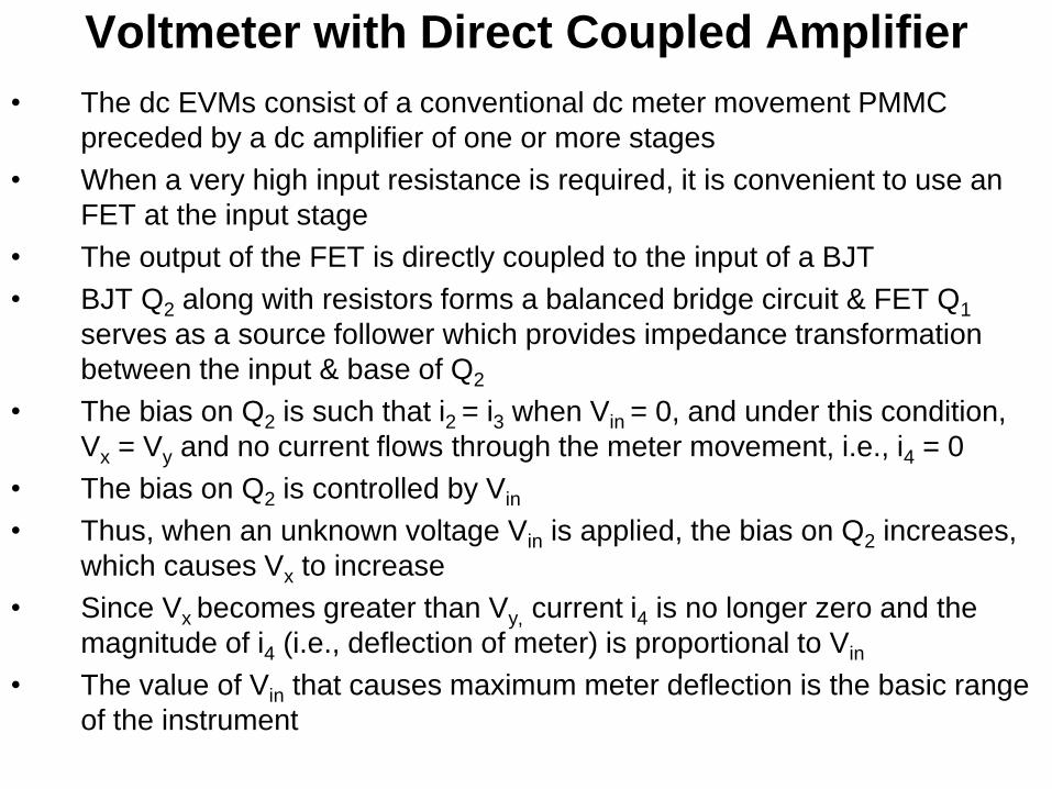
• The dc EVMs consist of a conventional dc meter movement PMMC

preceded by a dc amplifier of one or more stages

• When a very high input resistance is required, it is convenient to use an

FET at the input stage

• The output of the FET is directly coupled to the input of a BJT

• BJT Q2 along with resistors forms a balanced bridge circuit & FET Q1

serves as a source follower which provides impedance transformation

between the input & base of Q2

• The bias on Q2 is such that i2 = i3 when Vin = 0, and under this condition,

Vx = Vy and no current flows through the meter movement, i.e., i4 = 0

• The bias on Q2 is controlled by Vin

• Thus, when an unknown voltage Vin is applied, the bias on Q2 increases,

which causes Vx to increase

• Since Vx becomes greater than Vy, current i4 is no longer zero and the

magnitude of i4 (i.e., deflection of meter) is proportional to Vin

• The value of Vin that causes maximum meter deflection is the basic range

of the instrument

Voltmeter with Direct Coupled Amplifier

Voltmeter with Direct Coupled Amplifier (-contd.)

• This is, generally, the lowest range on the range switch in non-amplified

models

• Higher ranges can be obtained by using an input attenuator & lower ranges

can be obtained by preamplifier

• Bridge balance is obtained by adjusting the zero set potentiometer when

Vin = 0

• Full scale calibration is obtained by adjusting the potentiometer marked

calibration in series with ammeter

Advantages:

(i) It decreases the amount of power drawn from the circuit under test by

increasing the input impedance using an amplifier with unity gain

(ii) The source follower drives an emitter follower, and this combination is

capable of thousand fold or more increase in impedance while

maintaining a voltage gain of nearly unity

(iii) The input impedance of this meter is 10 MΩ, which requires a power of

0.025 µW for a 0.5 V deflection as compared to 25 µW for an unamplified

meter, thereby giving an increased sensitivity of 1000 times

Voltmeter with Direct Coupled Amplifier (-contd.)

• A block diagram of a meter used for measurement of small voltages &

currents is shown in fig. (20.18)

• The input voltage is amplified & applied to a meter (PMMC)

• If the amplifier has a gain of 10, the sensitivity of the measurement is also

increased by the same amount

• An amplifier capable of a fixed dc gain of 20 is not difficult to construct and

to keep stable

• A simple op-amp with required feedback components is suitable for this job

• But dc gains of much higher values (of the order of 106) are required to use

a standard PMMC movement to measure very small currents & voltages

such as nano-ampere & microvolt

• In theory, when large gains are desired, all the defects of the op-amp

become significant

• Offset current, offset voltage, and bias currents become so troublesome

that it is practically impossible to achieve acceptable performance with

standard op-amp

Amplified Voltage & Current Meter

Amplified Voltage & Current Meter (-contd.)

• The dc EVMs may be used to measure ac voltages by first

detecting the alternating voltage

• In some situations, rectification takes place before amplification

(as shown in fig. (20.23a))

• Here, the amplifier, ideally requires zero-drift characteristics and

unity voltage gain & a dc meter movement with sufficient

sensitivity

• In another method, rectification takes place after amplification (as

shown in fig.(20.23b))

• This method generally uses a high open-loop gain & large

negative feedback overcomes the non-linearity of the rectifier

diode

• AC voltmeters that uses half-wave or full-wave rectification are

usually of the average responding type, with the meter scale

calibrated in terms of the rms value of a waveform instead of the

average value

Electronic AC Voltmeter using Rectifiers

• Thus, most meters are calibrated in terms of both rms & peak

values

• Since most of the waveforms encountered in electronics are

sinusoidal; these methods are satisfactory & much less expensive

than a true rms-reading voltmeter

• However, non-sinusoidal waveforms will cause this type of meter

to read high or low, depending on the form factor (kf = Vrms /Vav ) of

the waveform

• The main advantage of the ac voltmeter is that using negative

feedback greatly reduces the response time

• In some cases, there may be requirement to measure the peak

value of a waveform instead of average value and the circuit of fig.

(20.24c) may be used for “peak” reading

• In most cases, the meter scale is calibrated in terms of both rms &

peak values of sinusoidal input waveform

Electronic AC Voltmeter using Rectifiers (-contd.)




• Selecting most appropriate instrument for a particular voltage instrument

depends on the performance required in a given situation

• Some important considerations in selecting a voltmeter are given below:

(i) Input Impedance, (ii) Voltage Ranges, (iii) Decibel Unit, (iv) Sensitivity

versus Bandwidth, (v) Battery Operation, & (vi) AC Current

Measurement

(i) Input Impedance:

• In order to avoid loading effects, the input resistance or impedance of the

voltmeter should be at least an order of magnitude higher than the

impedance of the circuit under measurement, e.g., when a voltmeter with

a 10 MΩ input resistance is used to measure the voltage across a 100 kΩ

resistor, the circuit is hardly disturbed & loading effect of the meter on the

circuit is negligible

• The same meter placed across a 10 MΩ resistor, however, seriously loads

the circuit and causes an error in measurement of approximately 30%

• The input impedance of the voltmeter is a function of the inevitable shunt

capacitance across the input terminals

Considerations in Selecting an Analog Voltmeter

• The loading effect of the meter is partly noticeable at the higher

frequencies, when the input shunt capacitance greatly reduces the

input impedance

(ii) Voltage Ranges:

• The voltage ranges on the meter scale may be in the 1-3-10

sequence with 10 dB of separation, or in the 1-5-15 sequence, or in

a single scale calibrated in dB

• In any case, the scale divisions should be compatible with accuracy

of the instrument, e.g., a linear meter with 1% full scale should have

100 divisions on the 1.0 V scale so that 1% can be easily resolved

• An instrument with an accuracy of 1% or less should also have

mirror backed scale to reduce parallax and to improve accuracy

(iii) Decibel Unit:

• Use of the decibel scale can be very effective in measurements that

cover a wide range of voltages


• For example, a measurement of this kind is found in the frequency

response curve of an amplifier or filter, where the output voltage is

measured as a function of the frequency of the applied input voltage

• Almost all voltmeters with dB scale are calibrated in dBm, referred

to some particular impedance

(iv) Sensitivity versus Bandwidth:

• As noise is a function of bandwidth, a voltmeter with a wide

bandwidth will pick up & generate more noise than one operating

over a narrow range of frequencies

• In general, an instrument with a bandwidth of 10 Hz to 10 MHz has

a sensitivity of 1 mV

• A voltmeter whose bandwidth extends only to 5 MHz could have

sensitivity of 100 µV


(v) Battery Operation:

• For field work, a voltmeter powered by an internal battery is

essential

• If an area contains troublesome ground-loops, a battery powered

instrument is preferred over a mains powered voltmeter to remove

the ground paths

(vi) AC Current Measurements:

• Current measurements can be made by a sensitive ac voltmeter

and a series resistance

• In the usual case, however, an ac current probe is used which

enables the operator to measure an ac current without disturbing

the circuit under test


Digital Voltmeter (DVM)

• A DVM displays the value of ac or dc voltage being measured

directly as discrete numerals in the decimal number system

• Numerical readout of DVM is advantageous since it eliminates

observational errors (e.g., parallax & approximation errors)

committed by operators

• The use of DVMs increases the speed with which readings can be

taken

• Also the output of DVMs can be fed to memory devices for storage

& future computations

• On account of developments in IC technology, the size, the power

requirements, & the cost of DVM have been reduced

• Because of small size, the portability of DVM has been increased

• In fact, for the same accuracy, a DVM is now less costly than its

analog counterpart

Types of DVMs

• Some of the most usually used DVMs are:

(i) Ramp Type DVM, (ii) Integrating Type DVM, & (iii) Successive

Approximation Type DVM

(i) Ramp Type DVM:

• The operating principle of a ramp type DVM is to measure the time that

a linear ramp voltage takes to change from level of input voltage to 0

voltage (or vice versa)

• The time interval is measured with an electronic time interval counter &

the count is displayed as a number

• At the start of measurement, a negative going ramp voltage (as shown

in fig. 28.41) is initiated but a positive going ramp may also be used

• The ramp value is continuously compared with the voltage being

measured (unknown voltage)

• At the instant, the value of ramp voltage is equal to that of unknown

voltage, a coincidence circuit (input comparator), generates a pulse

which opens a gate

• The ramp voltage continues to decrease till it reaches ground level

(zero volt), at which instant another comparator (called ground

comparator) generates a pulse & closes the gate

• The time elapsed between opening & closing the gate is „t‟ as

indicated in fig. (28.41)

• During this time interval, pulses from a clock pulse generator pass

through the gate and are counted & displayed

• The decimal number displayed by the readout is a measure of the

value of the input voltage

• The sample gate multivibrator determines the rate at which the

measurement cycles are initiated

• The sample gate circuit provides an initiating pulse for the ramp

generator to start its next ramp voltage

• At the same time, it sends a pulse to the counters which sets all of

them to 0, which momentarily removes the digital display of the

readout

Ramp Type DVM (-contd.)

Ramp Type DVM (-contd.)

Integrating Type DVM • Integrating type DVM measures the true average value of the input

voltage over a fixed measuring period

• This voltmeter employs an integration technique which uses a voltage

to frequency conversion

• The voltage to frequency (V/F) converter functions as a feedback

control system which governs the rate of pulse generation in

proportion to the magnitude of input voltage

• Actually when we use the voltage to frequency conversion technique,

a train of pulses (whose frequency depends upon the voltage being

measured), is generated

• Then the number of pulses appearing in definite interval of time is

counted

• Since the frequency of these pulses is a function of unknown voltage,

the number of pulses counted in that period of time is an indication of

the input (unknown) voltage

• The heart of this technique is the operational amplifier acting as an

integrator

Integrating Type DVM (-contd.)

• Output voltage of integrator is given by

• Thus if a constant input voltage Ei is applied , an output voltage Eo is

produced which rises at a uniform rate and has a polarity opposite to

that input voltage

• In other words, it is clear from the above relationship, that for a

constant input voltage the integrator produces a ramp output voltage

of opposite polarity

• Let us examine fig. (28.43), here the graphs showing relationships

between input voltages of three different values and their respective

output voltages are shown

• It is clear that polarity of the output voltage is opposite to that of input

voltage, not only that , the greater the input voltage the sharper is the

rate of rise (or slope) of output voltage

• The basic block diagram of a typical integrating type of DVM is shown

in fig. (28.44)

t.RC

E-dtE

RC

1- E i

io


• The unknown voltage (Ei) is applied to the input of the integrator, and

the output voltage (Eo) starts to rise

• The slope of Eo is determined by the value of Ei

• This voltage is fed to a level detector and when Eo reaches certain

reference level, the detector sends a pulse to the pulse generator

gate

• The level detector is a device similar to a voltage comparator, in

which the output voltage from integrator Eo is compared with the fixed

voltage of an internal reference source , and when Eo reaches that

level , the detector produces an output pulse

• It is evident that greater the value of input voltage Ei, the sharper will

be the slope of output voltage Eo, and quicker Eo will reach its

reference level

• The output pulse of the level detector opens the pulse generator

gate, permitting pulses from a fixed frequency clock oscillator to pass

through pulse generator


• The pulse generator is a device such as a Schmitt trigger, that

produce an output pulse of fixed amplitude and width for every pulse

it receives

• This output pulse (whose polarity is opposite to that of Ei and has a

greater amplitude) is fed back to the input of the integrator, & the net

input to the integrator is now of the reversed polarity as in fig. (28.45)

• As a result of this reversed input, the output Eo drops back to its

original level

• Since, Eo is now below the reference level detector, there is no output

from the detector to the pulse generator gate & gate gets closed

• Thus, no more pulses from the clock oscillator pass through to trigger

the pulse generator

• When, the output voltage pulse from the pulse generator has passed,

Ei is restored to its original value



Successive Approximation Type DVM

• The block diagram of the successive approximation DVM is shown in

fig. (5.10)

• When the start pulse activates the control circuit, the SAR is cleared

(i.e., the output of SAR is 00000000) and Vout of D/A converter is 0

• Now, if Vin > Vout , the comparator output is +ve

• During the first clock pulse, the control circuit sets the D7 to 1; Vout

jumps to Vref /2 and SAR output is 10000000

• If Vout > Vin , the comparator output is –ve and the control circuit

resets D7

• However, if Vin > Vout , the comparator output is +ve and the control

circuit keeps D7 set

• Similarly, the rest of the bits beginning from D7 to D0 are set & tested

• Hence, the measurement is completed in 8-clock pulses

• At the beginning of the measurement cycle, a start pulse is applied to

the start/stop multivibrator, which sets 1 in the MSB and 0 in all other

bits of the SAR (i.e., the reading would be 10000000)

Successive Approximation Type DVM

• The ring counter then advances one count, shifting a 1 in the second

MSB of the SAR and its reading becomes 11000000

• This causes the DAC to increase its output by Vref /4

(i.e.,Vout=Vref/2+Vref /4), and again it is compared with Vin

• In this case, Vout > Vin , the comparator produces an output that

causes the control circuit to reset second MSB of SAR to 0

• The DAC output (Vout) then returns to its previous value of Vref/2 and

awaits another input from SAR

• When the ring counter advances by 1, the third MSB is set to 1 and

the Vout rises by Vref /8 (i.e.,Vout=Vref/2+Vref /8)

• The measurement cycle, thus proceeds through a series of

successive approximations

• Finally, when the ring counter reaches its final count, the

measurement cycle stops & the digital output of the SAR represents

the final approximation of the unknown input voltage (Vin)

Successive Approximation Type DVM (-contd.)

Successive Approximation Type DVM (-contd.)

Digital Frequency Meter • The signal whose frequency is to be measured is converted into the

train of pulses, one pulse for each cycle of signal

• Then the number of pulses appearing in a definite interval of time is

counted by means of an electronic counter

• Since the pulses represent the cycles of unknown signal, the number

appearing on the counter is a direct indication of frequency of the

unknown signal

BASIC CIRCUIT:

• The block diagram of the basic circuit of a digital frequency meter is

shown in fig. (28.33)

• The unknown frequency signal is fed to Schmitt trigger through an

amplifier

• In the Schmitt trigger, the signal is converted into a square wave with

very fast rise and fall times, then differentiated and clipped

• As a result, the output from a Schmitt trigger is a train of pulses, one

pulse for each cycle of the signal

• The output pulses from the Schmitt trigger are fed to start stop gate

• When this gate opens (start), the input pulses pass through this gate

and are fed to an electronic counter which starts registering the input

pulses

• When the gate is closed (stop), the input of pulses to counter ceases

and it stops counting

• The counter displays the number of pulses that have passed through

it in the time interval between start and stop

• If the interval is known, the pulse rate and hence the frequency of the

input signal can be known

• Suppose f is the frequency of unknown signal, N the number of

counts displayed by counter, and t is the time interval between start

and stop gate

• Therefore, frequency of unknown signal is given by

Digital Frequency Meter (-contd.)

t

Nf

TIME BASE SELECTOR:

• It is abundantly clear that in order to know the value of frequency of

input signal, the time interval between start and stop of gate must be

accurately known

• This time interval known as time base can be determined by circuit

given in fig. (28.34)

• The time base consists of a fixed frequency crystal oscillator (known

as clock oscillator) and must be very accurate

• In order to ensure its accuracy, the crystal is enclosed in a constant

temperature oven

• The output of this constant frequency oscillator is fed to the Schmitt

trigger which converts the input to an output consisting of a train of

pulses at a rate equal to the frequency of the clock oscillator

• The train of pulses then passes through a series of frequency decade

divider assemblies connected in cascade


• Each decade divider consists of decade counter and divides the

frequency by 10

• Connections are taken from the output of each decade in series

chain, and, by means of selector switch, any output may be selected

• In the block diagram of fig. (28.34), the clock oscillator frequency is

1 MHz

• Thus the output of Schmitt trigger is 106 pulses per second and thus

the time interval between two consecutive pulses is 1 µs

• At x10-1 tap, the pulses (having gone through decade divider-1) are

reduced by a factor 10, and now there are 105 pulses per second

• Therefore the time interval between them is 10 µs

• Similarly, there are other time intervals at the output of respective

taps

• This time interval between the pulses is the time base and it can be

selected by means of the selector switch


Circuit for Measurement of Frequency:

• As shown in fig. (28.35), the +ve pulses from the unknown

frequency source (called counted signal) are arriving at input-A of

the main gate & the +ve pulses from time base selector switch are

arriving at the input-B of the start/stop gate

• Initially, FF-1 is in its 1 state

• The resulting voltage from output Y, applied to input-A of the stop

gate opens this gate and 0 V from output Ỹ of FF-1,applied to

input-A of start gate closes that gate

• As the stop gate is opened, the +ve pulses from the time base,

can get through to set input S of FF-2 & keep it in state 1

• The resulting 0 output voltage from Y is applied to input-B of main

gate, and no pulses from the unknown frequency source can pass

through the main gate


• In order to start the operation, a +ve pulse (called read pulse) is

applied to reset R of FF-1; which causes FF-1 to reverse its state

from 1 to 0

• Now, output Y of FF-1 is 0 and output Ỹ is +ve voltage; as a result,

the stop gate is closed & start gate is opened

• The same pulse is applied to the decades of the counters bringing

them to 0 and thus count can start now

• When the next pulse from the time base arrives, it is able to pass

through the start gate to reset R of FF-2 flipping it from state 1 to 0

• The resulting +ve voltage from its output Ỹ (called gating signal) is

applied to input-B of main gate, opening that gate

• Now, the pulses from unknown frequency source are able to pass

through and are registered on the counter

• The same pulse that passes through the start gate is applied to the

input S of FF-1 changing it state from 0 to 1


• This results in closing of start gate & stop gate is opened

• However, since main gate is still open, pulses from the unknown

frequency source continue to get through to the counter

• The next pulse from the time base selector passes through the

stop gate to the input S of FF-2 changing it back to its 1 state

• Its output from Ỹ becomes 0 and so the main gate is closed and

the counting stops

• Thus, the counter registers the number of pulses passing through

the main gate in the time interval between two successive pulses

from the time base selector, e.g., if time base selected is 1 s then

the number indicated on the counters will be the frequency of the

unknown frequency source in Hz

• The assembly consisting of the two AND gate & the two FFs is

known as Gate Control Flip Flop



From Time Base


Simplified Composite Circuit of Digital

Frequency Meter

• As shown in fig. (28.36), the principle of operation is same as that

described for “Circuit for Measurement of Frequency” in the

previous section

• There are two signals to be traced:

(i) Input Signal (or counted signal): the frequency of which to be

measured

(ii) Gating Signal (or counting signal): this determines the length of

time during which the counters are allowed to totalize the pulses

• The input signal is amplified and is applied to a Schmitt trigger

where it is converted to train of pulses

• A selector switch allows the time interval to be selected from 1µs

to 1s

Simplified Composite Circuit of Digital

Frequency Meter (-contd.)

• The first output from the time base selector switch passes through

the Schmitt trigger to the gate control flip flop

• The gate control flip flop assumes a state such that an enable signal

is applied to the main gate

• The main gate being an AND gate, the input signal pulses are

allowed to enter the DCAs (Decade Counter Assemblies) where they

are totalized and displayed

• This process continues till a second pulse arrives at the control gate

FF from DDAs (Decade Divider Assemblies)

• The control gate reverses its status, which removes the enabling

signal from the main gate & no more pulses are allowed to go to

counting assemblies since the main gate closes

• Thus, the number of pulses which have passed during a specific time

are counted & displayed on the DCAs


Time Period Measurement

• Sometimes, it is desirable & necessary to measure the period of an

input signal rather than its frequency

• This is specially true when measuring the low frequencies because

low frequency range using frequency mode of operation gives low

accuracy

• To get good accuracy, we should measure the time period (T = 1/f) to

know the unknown frequency (f) rather than make direct frequency

measurement

• Thus the period (T) measurement can be done directly by

interchanging the two input signals to the main gate

• The circuit for measurement of frequency in fig. (28.36) can be used

for measurement of time period but the counted & the gating signals

are interchanged

• Fig. (28.37) shows the circuit for measurement of time period

• The gating signal is derived from unknown input signal which now

controls the opening and closing of the main gate

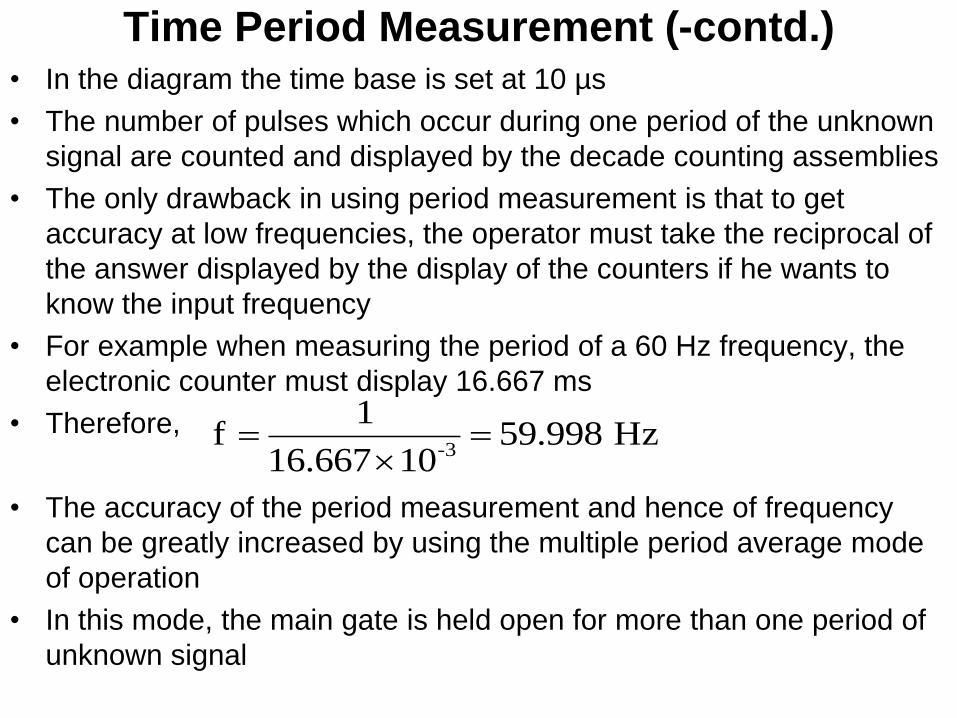
• In the diagram the time base is set at 10 µs

• The number of pulses which occur during one period of the unknown

signal are counted and displayed by the decade counting assemblies

• The only drawback in using period measurement is that to get

accuracy at low frequencies, the operator must take the reciprocal of

the answer displayed by the display of the counters if he wants to

know the input frequency

• For example when measuring the period of a 60 Hz frequency, the

electronic counter must display 16.667 ms

• Therefore,

• The accuracy of the period measurement and hence of frequency

can be greatly increased by using the multiple period average mode

of operation

• In this mode, the main gate is held open for more than one period of

unknown signal

Hz998.5910 16.667

1f

3-

Time Period Measurement (-contd.)

• This is done by passing the unknown signal through one or more

decade divider assemblies (DDAs), so that the period is extended

by a factor of 10, 100, or more

• Hence the digital display on the counters will show more digits of

information thus increasing the accuracy

• However, the decimal point location and measurement units are

usually changed each time an additional decade divider is added so

that the display is always in terms of the period of 1 cycle of the

input signal, even though the measurement may have lasted for 10

or 100 or more cycles

• Fig. (28.37) also shows the multiple period average mode of

operation by the dashed portion of the block diagram

• In this diagram, 5 more DDAs have been added so that the gate

now remains open for an interval of 105 times than it did with that

only one DDA



Time Interval Measurement

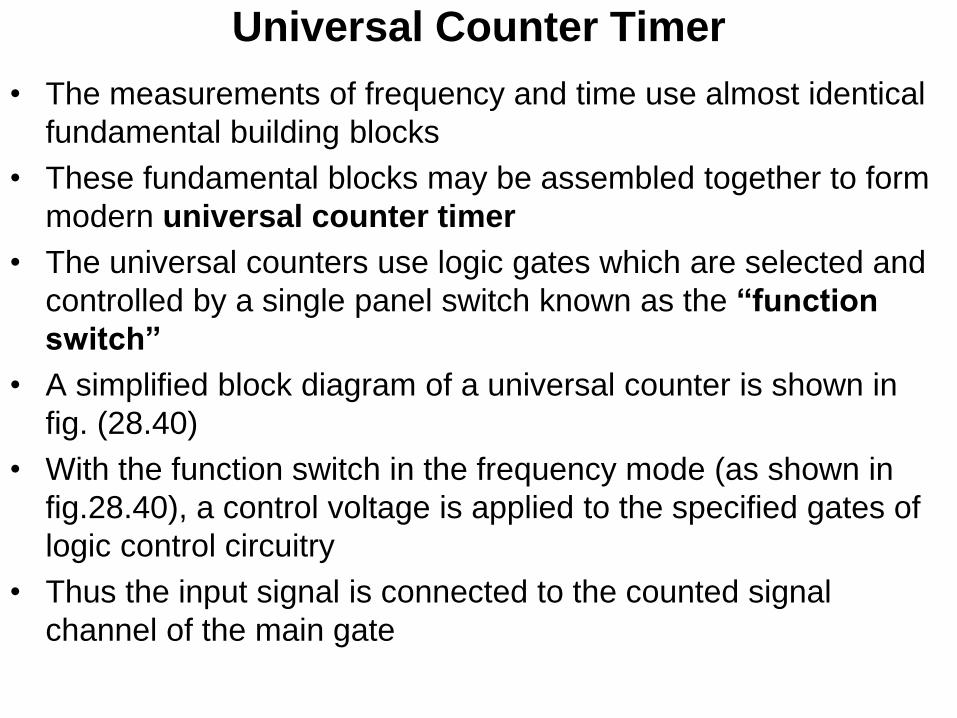
• The measurements of frequency and time use almost identical

fundamental building blocks

• These fundamental blocks may be assembled together to form

modern universal counter timer

• The universal counters use logic gates which are selected and

controlled by a single panel switch known as the “function

switch”

• A simplified block diagram of a universal counter is shown in

fig. (28.40)

• With the function switch in the frequency mode (as shown in

fig.28.40), a control voltage is applied to the specified gates of

logic control circuitry

• Thus the input signal is connected to the counted signal

channel of the main gate

Universal Counter Timer

• The selected output from the time base dividers is

simultaneously gated to the control flip flop , which enables or

disables the main gate

• Both control paths are latched internally to allow them to

operate only in the proper sequence

• When function switch is in Period mode, the control voltage is

connected to proper gates of logic circuitry ,which connect the

time base signal to the counted signal channel of the main gate

• At the same time the logic circuitry connects the input to the

gate control for enabling or disabling the main gate

• The other function switches (like time interval, ratio, external

standard) perform similar functions

• The exact details of switching and control procedures vary from

instrument to instrument

Universal Counter Timer (-contd.)

Universal Counter Timer (-contd.)

Date post:	04-Jul-2020
Category:	Documents
Upload:	others
View:	2 times
Download:	0 times

ELECTRONIC INSTRUMENTATION & CONTROL SYSTEMS (WLE … › emp › studym › 3231.pdf ·...

Documents