ELECTRONIC JOURNAL OF INTERNATIONAL GROUP ON RELIABILITY JOURNAL IS REGISTERED IN THE LIBRARY OF THE U.S. CONGRESS ● ISSN 1932-2321 ● VOL.2 NO.3 (14) SEPTEMBER, 2009 San Diego Gnedenko Forum Publications
Chakravarthy Srinivas (USA) e-mail schakravketteringedu Dimitrov Boyan (USA) e-mail BDIMITROKETTERINGEDU Genis Yakov (USA) e-mail yashag5yahoocom Kołowrocki Krzysztof (Poland) e-mail katmatkkamgdyniapl Krishnamoorthy Achyutha (India) e-mail krishnaakgmailcom Levitin Gregory (Israel) e-mail levitinieccoil Limnios Nikolaos (France) e-mail NikolaosLimniosutcfr Nelson Wayne (USA) e-mail WNconsultaolcom Popentiu Florin (UK) e-mail FlPopentiucityacuk Rykov Vladimir (Russia) e-mail rykovrykov1insru Wilson Alyson (USA) e-mail agwlanlgov Wilson Simon (Ireland) e-mail swilsontcdie Yastrebenetsky Mikhail (Ukraine) e-mail ma_yastrebmailru Zio Enrico (Italy) e-mail zioipmce7cesnefpolimiit
Technical assistant
Ushakov Kristina e-mail kudesignsyahoocom
e-Journal Reliability Theory amp Applications publishes papers reviews memoirs and bibliographical materials on Reliability Quality Control Safety Survivability and Maintenance
Theoretical papers have to contain new problems
finger practical applications and should not be overloaded with clumsy formal solutions
Priority is given to descriptions of case studies General requirements for presented papers 1 Papers have to be presented in English in
MSWord format (Times New Roman 12 pt 15 intervals)
2 The total volume of the paper (with illustrations) can be up to 15 pages
3 А presented paper has to be spell-checked 4 For those whose language is not English we
kindly recommend to use professional linguistic proofs before sending a paper to the journal
The Editor has the right to change the paper title and make editorial corrections
The authors keep all rights and after the publication can use their materials (re-publish it or present at conferences)
Publication in this e-Journal is equal to publication in other International scientific journals
Papers directed by Members of the Editorial Boards are accepted without referring
The Editor has the right to change the paper title and make editorial corrections
The authors keep all rights and after the publication
can use their materials (re-publish it or present at conferences)
Send your papers to
the Editor-in-Chief Igor Ushakov
igorushakovgmailcom
or
the Deputy Editor Alexander Bochkov
abochkovgmailcom
Table of Contents
RampRATA 3 (Vol2) 2009 September
- 5 -
Table of Contents
V Raizer NATURAL DISASTERS AND STRUCTURAL SURVIVABILITY 7 The term ldquodisasterrdquo is known to denote any environmental changes putting human lives under treat or materially deteriorating living conditions A considerable part of disasters comprises natural calamities These disasters can originate inside Earth (earthquakes volcanic processes) near or on its surface (disturbance of slope stability karsts considerable changes in soil conditions and groundrsquos settlements) The causes of disasters can as well be associated with a water either at a liquid (flood tsunami) or at a frozen state (complex or glacier avalanches) and finally with atmospheric conditions In many cases successions of interdependent disasters are possible including these occurring in different media (earthquake-tsunami earthquake-landslide and lands-flood etc) Gasanenko V A Chelobitchenko O O DYNAMIC MODEL OF AIR APPARATUS PARK 17 The article is devoted to construction and research of dynamic stochastic model of park of aircrafts A stochastic is enclosed in all of natural characteristic exploitations of this set of apparatuses times of flight and landing possibility of receipt of damage on flight including the past recovery air apparatus times of repair The estimations of total possible flights are got for the any fixed interval of time
Tsitsiashvili GSh Losev AS AN ASYMPTOTIC ANALYSIS OF A RELIABILITY OF INTERNET TYPE NETWORKS 25 In this paper a problem of a construction of accuracy and asymptotic formulas for a reliability of internet type networks is solved Analogously to [1] such network is defined as a tree where each node is connected directly with a circle scheme on a lower level with ngt0 nodes A construction of accuracy and asymptotic formulas for probabilities of an existence of working ways between each pair of nodes of the internet type network is based on a recursive definition of these networks and on asymptotic formulas for a reliability of a random port This asymptotic formula represents the port reliability as a sum of probabilities of a work for all ways between initial and final nodes of this port An estimate of a relative error and a complexity of these asymptotic calculations for a radial-circle scheme are shown Salem Bahri Fethi Ghribi Habib Ben Bacha A STUDY OF ASYMPTOTIC AVAILABILITY MODELING FOR A FAILURE AND A REPAIR RATES FOLLOWING A WEIBULL DISTRIBUTION 30
The overall objective of the maintenance process is to increase the profitability of the operation and optimize the availability However the availability of a system is described according to lifetime and downtime It is often assumed that these durations follow the exponential distribution The work presented in this paper deals with the problem of availability modeling when the failure and repair rates are variable The lifetime and downtime were both governed by models of Weibull (the exponential model is a particular case) The differential equation of the availability was formulated and solved to determine the availability function An analytical model of the asymptotic availability was established as a theorem and proved As results deduced from this study a new approach of modeling of the asymptotic availability was presented The developed model allowed an easy evaluation of the asymptotic availability The existence of three states of availability for a system has been confirmed by this evaluation Finally these states can be estimated by comparing the shape parameters of the Weibull model for the failure and repair rates Igor Ushakov Sumantra Chakravarty OBJECT ORIENTED COMMONALITIES IN UNIVERSAL GENERATING FUNCTION FOR RELIABILITY AND IN C++ 43 The main idea of Universal Generating Function is exposed in reliability applications Some commonalities in this approach and the C++ language are discussed
Table of Contents
RampRATA 3 (Vol2) 2009 September
- 6 -
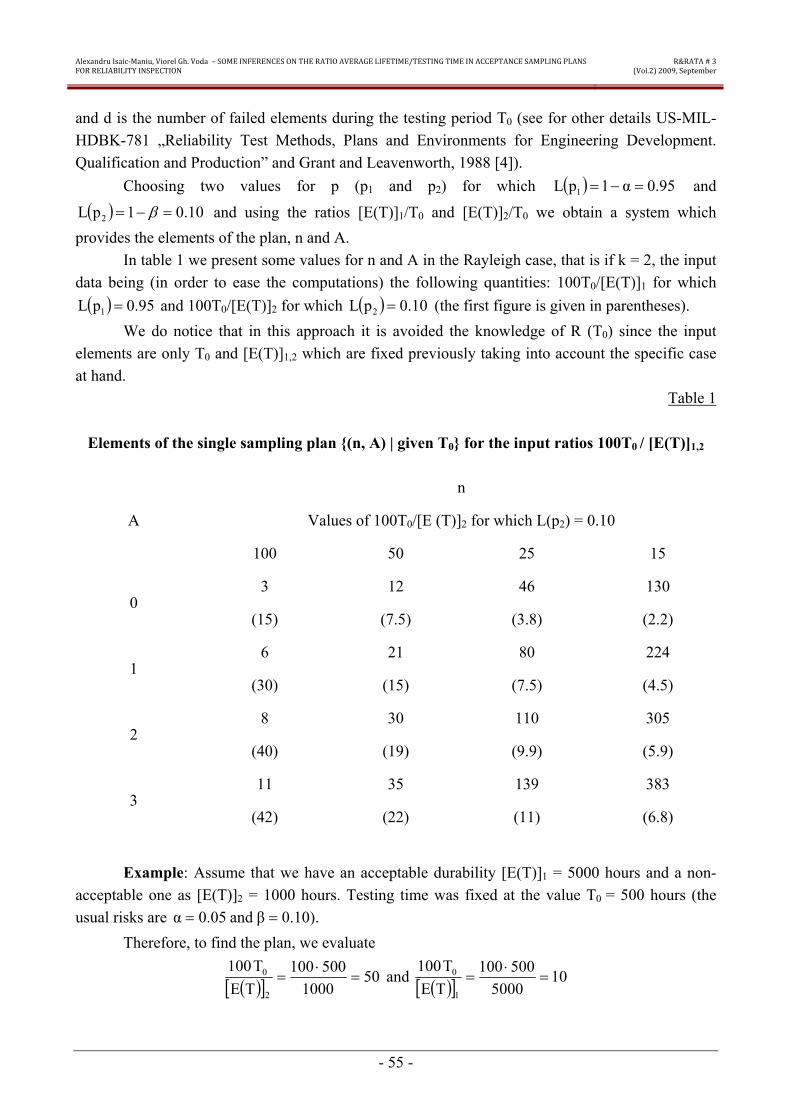
Alexandru ISAIC-MANIU Viorel Gh VODĂ SOME INFERENCES ON THE RATIO AVERAGE LIFETIMETESTING TIME IN ACCEPTANCE SAMPLING PLANS FOR RELIABILITY INSPECTION 51 In this paper we construct effective single sampling plans for reliability inspection when the distribution of failure times of underlying objects obey a Weibull law To this purpose we use the index average lifetime (E (T)testing time (T) for two values of E(T) - acceptable and non acceptable ones - and known shape parameter (K) of the Weibull cdf We derive also a relationship between this index and reliability function R(t) of the assumed statistical law A numerical illustrations is provided in the case of Rayleigh cdf - that is for a Weibull shape k = 2 Tsitsiashvili GSh Losev AS AN ACCURACY OF ASYMPTOTIC FORMULAS IN CALCULATIONS OF A RANDOM NETWORK RELIABILATY 58 In this paper a problem of asymptotic and numerical estimates of relative errors for different asymptotic formulas in the reliability theory are considered These asymptotic formulas for random networks are similar to calculations of Feynman integrals A special interest has analytic and numerical comparison of asymptotic formulas for the most spread Weibull and Gompertz distributions in life time models In the last case it is shown that an accuracy of asymptotic formulas is much higher
V Raizer ndash NATURAL DISASTERS AND STRUCTURAL SURVIVABILITY
RampRATA 3
(Vol2) 2009 September
- 7 -
NATURAL DISASTERS AND STRUCTURAL SURVIVABILITY
V Raizer
San Diego CA
1 PROBLEM OF DISASTERrsquoS PREDICTION
The term ldquodisasterrdquo is known to denote any environmental changes putting human lives under treat or materially deteriorating living conditions A considerable part of disasters comprises natural calamities These disasters can originate inside Earth (earthquakes volcanic processes) near or on its surface (disturbance of slope stability karsts considerable changes in soil conditions and groundrsquos settlements) The causes of disasters can as well be associated with a water either at a liquid (flood tsunami) or at a frozen state (complex or glacier avalanches) and finally with atmospheric conditions In many cases successions of interdependent disasters are possible including these occurring in different media (earthquake-tsunami earthquake-landslide and lands-flood etc) The analysis of conditions associated with the onset and the development of the dangerous natural processes becomes at present the subject of both the natural research and the engineering analysis New cities industrial power and other facilities are mostly erected in areas where natural calamities emerge Environmental changes of natural or man-caused origin lead to disastrous effects in areas developed earlier too It is always that the mechanisms of the dangerous natural phenomena can be represented by the direct cause-and ndashthe effect relations A prediction of the type the time and the size of the expected disaster even if practicable can only be probabilistic Therefore for the analysis of the structures for the areas where natural calamities can take place the probabilistic approach and the use of the reliability theory can prove to be more efficient and necessary than in regular cases The level of the development of many problems concerning the comprehension of natural calamityrsquos origination and hence the level of the efficiency in predicting their time conditions and the character of manifestation as well as the development of measures for their prevention and mitigation of losses leg behind with the practical needs of the national economy To a certain extent it can be accounted for by absence of common approaches to the constructing models of some natural disasters and the methods of their prediction To predict future events using statistical methods we should dispose of information for rather a long time period Practically however the prediction is based on limited information due to which it is often imprecise and sometimes merely incorrect Prediction accuracy however fluctuates within a certain range if the prediction is based on statistics alone It implies that different methods should also be employed in prediction For sufficiently substantiated prediction the following methods are generally used [2-6] malty-dimensional regression analysis theory of quantitative analysis graph theory for error analysis Delphi method (method of expert evaluation) and statistical analysis The latest research in the field of forecasting disastrous events and preventing the maximum risk and losses due to abnormal actions have shown that ever more widespread together with the foregoing five methods is becoming the approach based on the theory of fuzzy sets [7] This can be accounted for by the fact that any classification any algorithm any rule of decision making any model (theoretical or calculated) can be correlated with its fuzzy analogue For example classification implies the breakdown of a totality of elements into classes or groups of similar elements Rigorous classification refers each element to a single definite class whereas
V Raizer ndash NATURAL DISASTERS AND STRUCTURAL SURVIVABILITY
RampRATA 3
(Vol2) 2009 September
- 8 -
according to fuzzy classification it can belong to different classes depending to on certain conditions The fuzzy classification is generally more realistic than the rigorous one The use of the theory of fuzzy sets permits to elaborate basing on fuzzy input data a certain optimum solution setting applicability borders
2 METHODOLOGICAL ASPECTS OF THE ANALYSIS
An engineering analysis proper is not aimed at evaluating of the probabilistic parameters that represent natural processes and in theory the engineer should obtain from experts in natural sciences properly represented statistical information The task of the engineer is to assess using this information a risk associated with a particular structure and to device measures of disaster protection of human life and property efficient terms of the data available In practice however similarly to the case of estimating disastrous windrsquos speed or waterrsquos pressure parameters for example when designing safe structures or estimating a stressed state of undisturbed soilrsquos mass engineers dealing with the theory of a structural analysis cannot count on obtaining the foregoing information ldquofrom the outsiderdquo Hence an independent statistical analysis of available information is required so that the data based on it should correspond to peculiarities involved in the engineering analysis Moreover sometimes it becomes necessary to describe in terms of these peculiarities mechanisms of natural phenomena and to reveal their quantitative characteristics determining the extent of a structural damage Another moment that should be born in mind is the comprehension that for not all natural disastrous effects structures can and must be designed and it is not always that engineering measures aimed to mitigating of the destructive effect of disasters can be designed and implemented Design procedures envisaged in disregarding disastrous effects of an artificial origin Similarly when for example developing the code of design with due regard for the natural disasters one should not tackle an unsolvable problem of an analysis for all types or levels of the foregoing effects In fact there is nothing new about it the same idea is employed in specifying the ldquoassumedrdquo seismicity for which the structures in the area are to be designed whereas a higher-level earthquake motion is considered a ldquobeyond-designrdquo occurrence Here the expected events can be classified as ldquodesignrdquo or ldquobeyond-designrdquo according to the level of motion Meanwhile referred to ldquobeyond-designrdquo cases are sometimes entire types of events hard to predict or even quite unpredictable occurrences as mentioned above It needs to be said that the formal division of seismic effects upon structures and occurrences associated with them into ldquodesignrdquo and ldquobeyond-designrdquo cannot be accepted unless their consequences will be taken into account We know that in structural design for regular loads the term ldquofailurerdquo is generally used to denote a random event of realization of one of its damage states The aim of a competent design consists in specifying of the structural parameters in a way that would exclude such failures due to design loads In the design for natural disasters however the requirement of the inadmissibility of the failure in the foregoing sense can hardly be fulfilled and it should therefore be replaced by the requirement of the structural non-destructibility Non-destructibility would imply the preservation of the main structurersquos member that would permit to retrofit the whole structure (building for example) There are some types of structures or buildings however for which the foregoing consideration doesnrsquot seem to be important As far as structures whose failure presents a global threat to the environment are concerned non-destructibility means in this case the prevention from the failure of structural members that contain or emit substances containing environment This however applies to a design situation As regards ldquobeyond-designrdquo situation special engineering solutions are seemingly required for the above structures The solutions should ensure even in the case of the most improvable and unpredictable effects spontaneous deviation from hazardous production processes and self-isolation of units containing detrimental or hazardous components
V Raizer ndash NATURAL DISASTERS AND STRUCTURAL SURVIVABILITY
RampRATA 3
(Vol2) 2009 September
- 9 -
3 STATITICAL EVALUATION OF NATURAL DISASTERS
The probabilistic approach proper employed in evaluating a possible level of any disastrous phenomenon in a particular area can also prove to be efficient and useful when the structure or soil are not supposed to be analyzed for the mentioned phenomenon Therefore when elaborating a probabilistic concept for natural disasters one should primarily consider in a general form the feasibility of using the statistical approach for representing the disastrous effects In principle the aim of the statistical analysis in terms of the problem being considered is the probabilistic prediction of the time and the place of a natural disaster or on the contrary for the given place and the service life of the structure ndash the probability of occurrence for the given period of a certain disasterrsquos type Generally speaking besides probabilistic prediction direct forecasting based on warning signs can be used Reliable warning signs however are often detected just before the disaster and cannot be taken into account in long-term prediction influencing engineering solution To have a prior notion of the frequency and the extent of disasters possible in a particular region is the reason for which statistical methods are to be used The analysis of observations for previous years can give the information of the frequency and parameters of disasters in the past Assuming the probability of such events to be invariable in time the same frequency that was in the past should be predicted for the future This extrapolation however can prove to be rather conventional since data obtained generally refer to a limited time range alone For this reason the processing of the available data should be based on specially developed statistical models whose physical correspondence to the phenomena under consideration make the extrapolation trustworthy Since natural disasters are this way or other extreme occurrences (earthquake orand tsunami of high intensity landslide of a great amount of soil karsts crater of a large diameter) their statistics has the character of ldquostatistics of rare phenomenardquo The Poissonrsquos distribution can be proposed in this case and the time character of the disasters manifestations can be represented by the Poissonrsquos process The specificity of the probabilistic approach to extreme values of the parameter referred to disastrous manifestations of the natural processes the Poissonrsquos or other distributions that represent the statistics of the extremes take place [8] The necessity in the accounting and description of the parameters of three-dimensional variability as well as in the study of this variability at different scale levels is essential in terms of the determining on the basis of observations regions where this danger should be allowed in the practical engineering analysis ie solving the task of micro-zoning For this purpose as well as for a more detailed prediction of threatening occurrences methods for optimum prediction of random fields should be employed Areas where dangerous phenomena can occur at intensity levels not yet realized (earthquake exceeding the design level karsts crater over allowed dimensions) can be determined and assessed be the testrsquos observations of the similar occurrences however of lower pre-ultimate intensity Meanwhile to say nothing of the abovementioned incomplete trustworthiness of extrapolation the notion of a somewhat mass scale of occurrences though less intensive but in any case similar to ldquodisastersrdquo is far for being always correct There are certainly other types of dangerous phenomena too whose uniform realizations in the given area are of rather a mass scale such are natural landslides or stonewalls on different slopes in mountainous areas or rock bursts in mining working statistical data of these can also be obtained Natural disasters of geotechnical origin however can be ldquouniquerdquo hence we must not rely upon full-scale data selection and processing ie upon the so-called ldquoobjective analysisrdquo
V Raizer ndash NATURAL DISASTERS AND STRUCTURAL SURVIVABILITY
RampRATA 3
(Vol2) 2009 September
- 10 -
A specific feature of natural disasters (and man-caused disasters too) is that they are practically in avoidable Natural disasters are characterized by power and uncontrollability Typical of man-cased events is that they result from the speedy development of super-modern technologies and a production whose management contains a weak link that is a man able to make with tragic consequences (Chernobyl for example) The main task here is to predict possible disasters localizing them and mitigating possible losses The design of any structure should be preceded by the analysis of all possible types of natural or man-caused disasters in terms of the probability of occurrence of the practicability of initiation of some secondary disasters of the practicability of the localization of the preventive measures not connected with design methods and at last of the damage in the case of occurrence
4 SAFETY CRITERIA OF UNIQUE STRUCTURES
Before dealing with safety criteria we should clarify the notion of a unique structure and natural or other effects that determining its vulnerability are detrimental for human health The notion of the structural uniqueness and that of the treat of the natural or other phenomena are interconnected Considering the structural safety in terms of the treat to human life and health we should not connect the uniqueness of the structure with its cost or with the expected material losses alone The uniqueness should as well be linked with the level of the treat for people irrespective of its probability and of factors causing it such as the function and the size of the considered building the character of productions the presence of the radioactive products etc Hence unique structures are those whose damage or collapse no matter how long their probability could be threaten the life and the health of people either inside or which is more often outside the building The foregoing definition of the structural uniqueness permits to refer to refer to such buildings projects of national economy (industry energy transport and others) and those of a social sphere whose damage and collapse would entail threat to human life and health Vulnerability of unique buildings exposed to disastrous natural effects and possibility of their damage or collapse depend on
bull The extent to which loads due to disastrous natural phenomena exceed standard loads bull The influence of secondary factors (explosions fires) due to disastrous natural phenomena bull The errors involved in the design analysis and the choice of location of a building and those
made at the stage of maintenance bull Poor workmanship the discrepancy between the strength characteristics of building
materials and the standards strength degradation in the course of the maintenance Analyzing structural vulnerability or safety it is expedient to single out the so-called ldquocriticalrdquo elements on which structural safety mostly depends For many structures such are the bearing members of the buildings that determine their strength and stability (foundation columns floors joints supports ets) For other buildings ldquocriticalrdquo elements will be those able to resist explosion or fire caused by natural cataclysms ensuring a reliable operation of safety systems For a number of unique buildings ldquocriticalrdquo elements are associated with the radioactivity or with the insurance of radiation safety Differences in the character of the critical elements require performing when choosing safety criteria of unique units a systematic analysis in order to find these elements and to assess the consequences of their failure The systematic analysis of structural safety should include the elaboration of the scenario of a natural effect taking into account the specificity of the latter the structure of the unique building the presence and the character of the ldquocriticalrdquo elements the consequences of their failure the nature of unitrsquos damage or collapse and their influence on the safety of people inside or outside the building and on the environment
V Raizer ndash NATURAL DISASTERS AND STRUCTURAL SURVIVABILITY
RampRATA 3
(Vol2) 2009 September
- 11 -
Generally speaking every natural phenomenon and every unique building require a scenario permitting to take their specificity into account and to obtain statistical data for generalizing the consequences The elaboration and the analysis of the scenarios require a great professional effort of people acquainted with the specificity of the branch and the particular unique building To specify qualitative and quantitative safety criteria of unique buildings exposed to any types of natural effects an integrated approach should be recommended as based on
bull Systematic deterministic analysis of scenarios of the influence of natural disastrous factors on concrete unique buildings revealing particular quality criteria
bull Probabilistic risk analysis determining particular and general probabilistic safety criteria that include those for limit states representing the extent of the failure and criteria for the personnel and other people in terms of the threat for human life and health (individual risk collective risk etc)
bull ldquoCost-benefitrdquo analysis to define more exactly safety basing on optimization of investments for protection against unfavorable effects with due regard for socio-economic factors
5 COMMENTS TO CODIFIED PROCEDURES
Among the codes on design of unique structures there are no codes of environment protection and the boundaries of homeostasis1of a living system as predominant in the process of determining the basis and analyzing structural strength stability durability This kind of code should specify a limit state in terms of environment protection in the result of investigation construction and maintenance of structures the interface in the space of environmental parameters separating their domain wherein a living system can exist from the rest part of the space should not surpass the boundary of the living systemrsquos homeostasis The transition from homeostatic domain through its boundary means the termination of the existence of given organism ie the given living system To ensure homeostasis it is required to determine its boundaries to be able to assess the position of the whole living system with respect to the specified homeostasis boundary eg to develop a specific informational system sensors gauges monitoring decision making procedures With codifying boundary protection and homeostatic boundaries of a unique structures living system particular attention should be paid to geo-pathogenic2 areas within the limits of design construction and maintenance Geo-pathogenous zones result from the heterogeneous3 structure of Earthrsquos Crust that anomalous information fields detrimental for the energy of bio-systems or objects of inanimate nature It is not advisable to assembly in the geo-pathogenous zones structures important in terms of economy and ecology Codes specifying the contents of designs of unique systems should contain the section of analysis and evaluation of damage or failure probability of the structure being designed This section should also contain appropriate scenarios for the operation of expert teams trained to eliminate damage localize ecological losses and to rescue people animals and the whole animate system in the region of disaster As concerns the abovementioned section national data bank should be complied and constantly replenished the data bank should contain information on the causes and the physical meaning of failures systematic analysis material and other losses and on methods of damage elimination and rescue of the animate system
1 Relatively stable state of equilibrium 2 This term was coming from the world of Dowsing 3 Derved from the Greek used to describe that has a large amount of variants
V Raizer ndash NATURAL DISASTERS AND STRUCTURAL SURVIVABILITY
RampRATA 3
(Vol2) 2009 September
- 12 -
Reliability is determined by the extent of structurersquos non-exposure to danger (in case under consideration to elemental natural and elemental man-cause disasters) it being impracticable and inexpedient here to guarantee structural survivability as regards all including almost improbable dangerous effects 6 STRUCTURAL SYSTEMrsquoS SURVIVABILITY4
Different situations in beyond-design states of structures can appear as a result of applying of natural or man-caused abnormal actions on building which have not been foreseen in design These states can be classified according to failure form degree of damage and final state The following forms of failure can be considered for ultimate limit state
bull Loss of strength in time of plastic brittle ductility or fatigue failure of elements bull Elastic or inelastic buckling of structures bull Loss of the stable equilibrium of the whole building
According to the degree of the intensity it can be bull Full progressive failure of the whole building Such form of a failure is typical for brittle
structures when a damage of separate elements can arouse dynamic effects in other elements of a structure
bull Little by little growing failure of accidental character as a result of plastic deformations accumulation This situation will stop exploitation and demands restoration This form of failure is typical for structures from elastic-plastic materials when failure of separate elements accompanies by growing of large displacements and redistributions of inner forces
It is useful to denote that failure analysis shows that practically always the process of structural failure is avalanche-like representing a sequence of failures of the members the is composed of in which case ldquofailurerdquo means both partial damage and complete failure In the overwhelming majority of cases however in individual failures do not bad to a total breakdown in a structure provided it is redundant stress redistribution takes place and the structure keeps performing its functions though perhaps not to the full capacity
This is favorable from the practice point of view the situation can be accounted for by bearing capacity reserves that the structures posses At present these margins are envisaged in the design as based on experience and intuition For achievement of an expedient reliability level the structure should be designed to bridge over a loss of a supporting member so that the area of damage is limited and localized [9]
It is but natural to use the word ldquosurvivabilityrdquo applicably of the structural system to preserve an ability to carry out the main functions in the period of accidental perturbation and do not permit the progressive collapse or the cascade development of failures Survivability is quite an important and applicably to unique and important structure indispensable property since reliable performance of structures is only possible if an appropriate level of survivability is ensured
There arises at once the question of this propertyrsquos quantitative aspect At present conventional is a probabilistic approach to structural reliability evaluation hence it is natural to employ it when obtaining numerical characteristics of survivability too Then in compliance with the general methods survivability level will be determined by a probability of some events characterizing the process of failure It is logical to consider how some critical state is attained in the process of successive failures of members This can be the failure of some numbers of members assigned in advance and the formation of an instantaneous mechanism or the failure of some isolated members etc Complying with this approach a structure can be considered to possess 4 The term integrity can be used too
V Raizer ndash NATURAL DISASTERS AND STRUCTURAL SURVIVABILITY
RampRATA 3
(Vol2) 2009 September
- 13 -
survivability if the probability of the above event for damaged structure is not so high as compared to its undamaged counterpart (other criteria can as well be used)
The index of survivability can be expressed in the following way
f
f
PP
=η (1)
Where fP -probability of failure of the designed system fP ndashprobability of failure of the
same system when some members failed Survivability factors η are in [01] interval The more is its value the larger is the reserve of survivability in structural system The steel frame is considered in Fig1
Fig1 Two-story frame
In the longitudinal direction framersquos span is 6m h = 4m All members of considered frame have I-sections with aria moments W = 615middot10-5m3 (1st floor column) W = 828middot10-5m3 (2nd floor column) W = 1270middot10-4m3 (1st floor girder) W = 1098middot10-4m3 (2nd floor girder)
Probabilistic analysis was performed taking into account random nature of applied loads and yield stress of framersquos material with given probability distributions Table 1 contains parameters of these distributions Calculations were made on the base of linear programming method (simplex method) with the application of the direct integration of distribution function [1011] Probability of failure is Pf =55110-5
Table 1
Random value Distribution Mean value Standard deviation s
Parameters of distribution
Design values
Wind load P1 P2
Gumbel 0144 2 кН м 0 037 2 кН м u кН м= 0127 2 z кН м= 0 029 2
0 2576 2 кН м
Snow load q3
Gumbel 11418 2 кН м 0 4681 2 кН м u кН м= 0 931 2 z кН м= 0 365 2
16 2 кН м
Load due to use q4
Gauss 0 88 2 кН м 0 21 2 кН м ndash 168 2 кН м
β = 14 3
V Raizer ndash NATURAL DISASTERS AND STRUCTURAL SURVIVABILITY
RampRATA 3
(Vol2) 2009 September
- 14 -
Random value Distribution Mean value Standard deviation s
Parameters of distribution
Design values
Yield point σy
Weibul 305 25 МПа 25МПа α = 316 42 МПа x0 0=
245МПа
More probable is the partial mechanism of failure when plastic hinges appear in cross-
sections 4 7 and 9 (Fig1) The values of the failure probabilities of considered frame are listed in Table 2 for different cases of cross-sections weakening
Table 2
section
s
Probability of failure Pf Lowering of aria moments W in different sections
From Table 2 follows that in the case of a failure of any cross-section probability of failure
for frame will not exceed the value 025580 =fP (the failure of cross-section 7) The failure of cross-section 7 will not lead to the collapse of all structure but essentially decreases its survivability Even the full failure of cross-sections 2 or 11 has no influence on probability of this frame The failure of the cross-section 1 2 17 or 18 has also no essential influence at this probability Survivability index of the considered frame with regard to the failure of cross-section 7 constitutes
002150025580
10515 5
=sdot
=minus
η
If in the process of structure exploiting some actions will be ensuring then the probability of the failure of the whole frame in case when one cross-section failed can be decreased to the value
0047710 =fP Survivability index will be
V Raizer ndash NATURAL DISASTERS AND STRUCTURAL SURVIVABILITY
RampRATA 3
(Vol2) 2009 September
- 15 -
011500047710
10515 5
=sdot
=minus
η
At Fig 2 graphs due to dependences between probability of failure and weakening of cross-sections 7 8 and 3 are presented
Fig 2 Dependence between fP and W
The process of developing and utilizing structures and structural members comprises numerous measures considered herein however are only those ensuring a required reliability level Different reliability levels are ensured through different cost of construction For structures in hazardous areas an expedient reliability level should be specified It should be determined the necessary safety guarantee of the structure and people The failure criterion assumed in the design of buildings for ordinary performance conditions is mainly that of serviceability
A reliability level for construction in hazardous areas should be that of failure ndashfree performance This should be an objective criterion determining the totality of codes control services and other measures that would ensure an expedient reliability level
REFERENCES
1 Freund R Wilson WSa P (2006) Regression Analysis Elsevier Science 480pp 2 Cramer D (2003) Advanced Quantities Data Analysis Open Univ Press 376pp 3 Gross JL (2005) Graph Theory and its Applications Wesley amp Sons 800pp 4 Aitkin CGG Taroni F(2004) Statistics and the Evaluation of Evidence for Forensic
Scientists (Statistic in Practice) JWeley amp Sons 540pp 5 Bedford T Cooke R (2001) Probabilistic Risk Analysis Foundations and Methods
Cambridge Univ Press 414pp 6 Calafiore G Dabbene F-Editors (2006) Probabilistic and Randomized Methods for Design
under Uncertainty Springer 457pp 7 Klir GJ Bo Yuan (1995) Fuzzy Sets and Fuzzy Logic Theory and Applications Prentice Hall
592pp 8 Gumbel EJ (1967) Statistics of Extremes Columbia University Press New York 9 Lew HS (2005) Best Practice Guidelines for Mitigation of Building Progressive Collapse
Building and Fire Research Laboratory National Institute of Standards and Technology Gaithersburg Maryland USA 20899-8611
V Raizer ndash NATURAL DISASTERS AND STRUCTURAL SURVIVABILITY
RampRATA 3
(Vol2) 2009 September
- 16 -
10 Raizer VD Mkrtychev OV ldquoNonlinear Probabilistic Analysis for Multiple-unit Systemsrdquo Proc 8th ASCE Specialty Conference on Probabilistic Mechanics July 2000Univ Notre-Dam IN
11 Mkptychev O V (2000) Reliability of Multiple-unit Barrsquos Systems of Engineering Structures Manuscript of doctorial thesis Moscow (in Russian) 493p
Gasanenko VA Chelobitenko OO ndash DYNAMIC MODEL OF AIR APPARATUS PARK
RampRATA 3
(Vol2) 2009 September
- 17 -
DYNAMIC MODEL OF AIR APPARATUS PARK
Gasanenko V A bull
Institute of Mathematics of National Academy of Science of Ukraine Tereshchenkivska 3 Kyev-4 Ukraine
e-mail gsimathkievua
Chelobitchenko O O bull
Center of Military-Strategic Investigations of National Academy of Defense of Ukraine Povitroflotsky prospect 28 Kyiv -49 Ukraine
e-mail chelobmailru
Abstract
The article is devoted to construction and research of dynamic stochastic model of park of
aircrafts A stochastic is enclosed in all of natural characteristic exploitations of this set of apparatuses times of flight and landing possibility of receipt of damage on flight including the past recovery air apparatus times of repair The estimations of total possible flights are got for the any fixed interval of time Key Words Flight time time on the ground recoverable damage loss of air apparatus repair time generating function renewal equation 1 INTRODUCTION
The important problem of management of the park of air apparatuses (PAA in short) maintenance as stage of their life cycle is an estimation of ability to provide the necessary amount of flights in given time interval of exploitation The dynamics of exploitation of every apparatus consists of alternation of times of flight times of repair and times of stand-down These times are determined both external requests on flights and different damages during flight or loss of air apparatus (AA in short) on flight Forecasting of the state of PAA is one of way of control of quality of management This approach may be realized by modeling [1] Analysis of literature in this direction shows that mainly authors develop of the models in a few lines The authors of line [2-4] simulate of control of technical state of PAA with aim the optimization of preventive maintenance with respect to restoration of PAA parameters The authors of next line [5-7] develop either methodological approach of operation adaptive control of technical state of PAA on basis of using of potential of corporative resources of unit information space (network-center environment) with purpose improving or support on the given level of reliable and durability indexes [5 6] or task of definition of optimal type of PAA taking into account economical indexes The authors of another line [8-10] build their own investigations on expert estimations In this case experience shows that decisions may be false Therefore it is urgency to develop models which first consider of change of state of PAA by different manner
Gasanenko VA Chelobitenko OO ndash DYNAMIC MODEL OF AIR APPARATUS PARK
RampRATA 3
(Vol2) 2009 September
- 18 -
Namely which are grounded on the following probability indexes probability of return of AA from flight without damages probability of to receive certain damages of AA in flight probability of to lose of AA in flight Analysis of interaction of these indexes of random events is not simple process
And so it is actually secondly a development of such models that are based on analytical dependence with more complex mathematical filling In the article approaches are offered to the solution of the following task We will designate through
in the amount of AA able to fly up in some i -th moment of time It is required to estimate of possibility to do given amount of flights Q in times of k successive time starts j - th 1+j -th L j -th starts In other words we must estimate possibility of implementation of relation
kjjj nnnQ ++ +++le L1 at any fixed integer j and k
2 It is assumed that N units of AA which are exploited from some initial moment of time For definiteness we suppose that all (able to fly) AA fly up and land at the simultaneously
Let us adopt the following notation We will denote by kτ the flight time after k -th takeoff and by kξ the time on the ground
after k -th landing Thus moments of takeoffs ls are defined recurrently
01 =s )(112 sum=
+=+=l
ok
kklss ξτξτ K
The moments of landing lt are defined analogy
11 τ=t )(1
2112 summinus
=
++=++=l
ok
kklltt ξτττξτ K
Further we will consider the following probabilities as result of flight of every AA Let us denote by 21 =ipi the probabilities to obtain (in flight) eliminated damages by 3p the probability of loss of AA in flight by 4p the probability to be safe and sound It is assume that 14321 =+++ pppp We will use symbols lβ and lα to denote the amount of AA at the minusl th takeoff ( minusl
th flight) and at the minusl th landing respectively The time of repair at the minusi th eliminated damage of the thk minus AA in the thl minus flight is
equal to a random variables )( lkid 1121 gelele= lki lβ with the distribution functions
( ) ( ))()( )(
22)(
11 xdPxFxdPxF lklk lt=lt=
We will introduce sequences of independent events )( lkiA 114321 lkli βlelege=
These events are connected with aircraft events in flight so that the following equalities take place ( ) ( ) i
lki
lki pAEIAP == )()( here )(sdotI denotes the indicator of events
In what follows we shall be assuming that random variables form ensemble
Gasanenko VA Chelobitenko OO ndash DYNAMIC MODEL OF AIR APPARATUS PARK
RampRATA 3
(Vol2) 2009 September
- 19 -
( ) 1 )()(2
)(1 ge=Π lkiAIdd lk
ilklk
ii ξτ
are independent in common Put
sum=
+=l
k
kkls
22 )( ξτ ( ) ( )sum
=
isin=2
1
1)1()1(
1 )0[i
ki
ki dIAIEr ξ
( ) ( )sum=
minus ++isin=2
121
121
)()( )[i
lllki
lkil ssdIAIEr ξξ 2gel
here and in the sequel we assume that 02 =ls if 2ltl
By hypothesis on independence
( )1)11(
2
1
1 ξlt=sum=
ii
i dPpr sum=
=2
1i
liil rpr 2gel
where ( )1
)11(1 ξlt= ii dPr ( ))[ 21
121
)11( llili ssdPr ++isin= minus ξξ 2gel
We introduce the generating functions
suminfin
=
=
1
)(m
mm bssB where mm Eb β= sum
infin
=
=
1
)(m
mm rssR ]10[isins
Theorem 1 The following formulas take place
)(1)(
4 sRspsNssBminusminus
= (1)
Proof We shall establish the stochastic relations for sequences mβ mα 1gem The designation
ζωw= means that random variables ω and ζ have the same distribution function
We will denote by A the complement of a set A
1 N=β sum=
⎟⎠⎞⎜
⎝⎛=
N
k
kwAI
1
)1(31α
Gasanenko VA Chelobitenko OO ndash DYNAMIC MODEL OF AIR APPARATUS PARK
RampRATA 3
(Vol2) 2009 September
- 20 -
( ) ( ) ( )1)1(
1
2
1
)1(
1
)1(42
11ξβ
ββ
lt+= sumsumsum= ==
ki
k i
ki
k
kwdIAIAI sum
=
⎟⎠⎞⎜
⎝⎛=
2
1
)2(32
β
αk
kwAI
M
( ) m
k
mkwm
mAI γβ
β
+= summinus
=
minus1
1
)1(4 sum
=
⎟⎠⎞⎜
⎝⎛=
m
k
mkwm AI
β
α
1
)(3
where ( ) ( )sumsumsumminus
=
minus
= =
minusorminusisin=1
1
1)(
1
2
1
)( )0[m
l
lmlmlk
ik i
lki
wm tstsdIAI
lβγ
The random value mγ is equal to amount of AA which finished the repairs in the interval of
time between thm minusminus1 and thm minus takeoffs By the construction of mβ we have the following relations
1 Nb = summinus
=
minusminus +=1
1
14
m
l
lmlmm rbbpb 2gem (2)
We introduce the functions
suminfin
=
=
1
)(m
mm bssB sum
infin
=
=
1
)(m
mm rssR ]10[isins
From the (1) we obtain
summinus
=
minusminus +=1
1
14
m
l
lmlm
mm
mm rbsbpsbs 2gem (3)
Summarizing left and right parts of (3) yields
)()()()( 4 sRsBssBpssNsB +=minus
From the latter one we get
)(1)(
4 sRspsNssBminusminus
=
Proof is completed Corollary Assume that the sequences from Π satisfy the conditions
Gasanenko VA Chelobitenko OO ndash DYNAMIC MODEL OF AIR APPARATUS PARK
RampRATA 3
(Vol2) 2009 September
- 21 -
1)(lim2
1)11( =
⎟⎟⎟
⎠
⎞
⎜⎜⎜
⎝
⎛++lt sum
=infinrarr
n
k
kkindP ξτξ 21=i Then the following equality is valid
31
pNb
mm =sum
ge
(4)
Proof Since random variables from Π are independent we have that
( )ni
i
i
n
l
ln sdPprR 21)11(
2
11
+lt== sumsum==
ξ (5)
Combining (1) (5) and condition from the Сorollary we get
nn
RRinfinrarr
= lim)1( = sum=
2
1iip
32141)1(
pN
pppNB =
minusminusminus=
The proof is completed 2
We shall formulate the problems of estimations of mb in terms of theory of renewal processes
Let us denote by 121 geisin ii Kκ the sequence of independent discrete random values with common distribution law ( ) 1411 1 rpP +=== κδ ( ) ll rlP === 1κδ 2gel
It is well known that if sum=
=k
i
ikS1
κ and min)( mSkm k ge=η then )(mEη 1gem is
unique solution of the renewal equation summinus
=
minus=1
1
)()(m
l
l lmEmE ηδη
Comparing latter one and (2) we conclude that )(mEbm η=
Let )()( 1 mPmG le= κ and sum+
=
=Mm
miibMmh )(
Now we obtain the following upper estimation
( ) ( ) ( )sumsumsumsumsumsum=
+
==
+
=
infin
= =
+le+le=+le=M
i
im
n
nM
i
im
n
n
n
M
i
n imGimSPimSPMmh0 10 11 0
)( (6)
Gasanenko VA Chelobitenko OO ndash DYNAMIC MODEL OF AIR APPARATUS PARK
RampRATA 3
(Vol2) 2009 September
- 22 -
Since ( )mi
ii sdPppmG 21
)11(2
14)( +lt+= sum
=
ξ 1gem the estimation (6) is well calculated
3
Now we will consider the construction of )(sB more detail for special case We make the following additional assumptions
minus kτ 1gek have the same distribution function with Laplace transformation exp)( 1τψ sEs minus= 0gts
minus kξ 1gek have the same distribution function with Laplace transformation exp)( 1ξϕ sEs minus= 0gts
minus )exp(1)( xxF ii λminusminus= 21=i
For convenience we put )()()( sssf ϕψ= Now we shall obtain more exact expression for )(sR By induction we shall calculate the lir for K21=l
Gasanenko VA Chelobitenko OO ndash DYNAMIC MODEL OF AIR APPARATUS PARK
RampRATA 3
(Vol2) 2009 September
- 23 -
sumsumsum=
infin
==⎪⎭
⎪⎬⎫
⎪⎩
⎪⎨⎧
minusminus
+minus==2
1
2
1
2
1)(1
))(1)(())(1()(
ii
iiii
mmi
m
ii fs
fssprspsR
λλλϕ
λϕ
Thus we have the following expression for this case
33
221
321
221
1
)()(
sasasa
sffsffsNsB
minus+minus
++minus= (7)
where for convenience we introduced notation )( ii ff λ= )( ii λϕϕ =
sum=
minus minusminusminusminus++=2
1
3214212 ))1(()(i
iiiii ffpffpffa ϕϕ
sum=
minusminusminus=2
1
32143 )(i
iiii ffpffpa ϕ
Thus in this case the term mb poses no problem because expression (7) can be expanded into the convergent power series about s
Further it is easy to check that under such special assumptions the function )(mG from Section 2 has the following form
)()()( 12
1
214 im
ii
mippppmG λψλϕ minus
=summinus++=
Remark It is clear that restriction on number of different types of eliminated damages (only
two) is not essentially The proved formulas are transformed for more number of types easy
REFERENCES
1 Borodin ОD (2006) Methodic approach to definition of output mount-quality composition of airplanes of fighting aircraft on data of estimations of changes of relation of forces of parties in operation Collect science works DNDIA ndash Кyiv DNDIA 2(9)pp12-17(in Ukrainian)
2 Vorobrsquoev VG Gluhov VV Kоzlov Yu V and etl (1984) Diagnostic and forecasting of technical state of aviation equipment Мoskow Transport (in Russian) 191pp
3 Manrsquoshin GG (1976) Control of regimes of precautions of complex systems Minsk Nauka i Techika (in Russian) 256pp
)1()1(2
1
2141 sum=
minus+++=
i
iipffpa ϕ
Gasanenko VA Chelobitenko OO ndash DYNAMIC MODEL OF AIR APPARATUS PARK
RampRATA 3
(Vol2) 2009 September
- 24 -
4 Smirnov NN Ickovich AA (1987) Service and Repair of aviation equipment with respect to state Мoskow Transport (in Russian) 272pp
5 Harchenko OV Chepizhenko VI (2006) The science problem of adaptive control of technical state of war aviation equipment of Ukraine in modern conditions Collect of Science Works of DNDIA ndash Кyiv DNDIA 2(9)pp6-11 (in Ukrainian)
6 Harchenko OV Pavlov VV Chepizhenko VI (2006) Conception of adaptive virtual control of technical state of war aviation equipment into network-center environment Collectof Science Works of DNDIA ndash Кyiv DNDIA 3(10)pp6-15 (in Ukrainian)
7 Harchenko OV Mavrenkov OE (2006) To question of ground of ration type of air apparatus park of war appropriation Collect Science Works of DNDIA ndash Кyiv DNDIA 4(11)pp6-9 (in Ukrainian)
8 Vasilrsquoev VN Zhitomirsky GI (1967) Probability foundations of military aviation complexes MoskowVVIA named prof NE Zhukovsky (in Russian) 164pp
9 Milrsquogram YuG Popov IS 1970 Military effectiveness of aviation equipment and operations researches MoskowVVIA named prof NE Zhukovsky (in Russian) 500pp
10 Tarakanov KV (1974) Mathematics and armed struggle Moskow Voenizdat (in Russian) 240pp
11 Cox DR Smith W L (1967) Renewall Theory Moskow ldquoSovetskoe Radiordquo (in Russian) 299pp
Tsisiashvili G Losev A ndash AN ASYMPTOTIC ANALYSIS OF A RELIABILITY OF INTERNET TYPE NETWORKS
RampRATA 3
(Vol2) 2009 September
- 25 -
AN ASYMPTOTIC ANALYSIS OF A RELIABILITY OF INTERNET TYPE NETWORKS
Tsitsiashvili GSh Losev AS
Institute for Applied Mathematics Far Eastern Branch of RAS 690041 Vladivostok Radio str 7 guramiamdvoru alexaxbkru
Introduction In this paper a problem of a construction of accuracy and asymptotic formulas for a reliability
of internet type networks is solved Analogously to [1] such network is defined as a tree where each node is connected directly with a circle scheme on a lower level with ngt0 nodes A construction of accuracy and asymptotic formulas for probabilities of an existence of working ways between each pair of nodes of the internet type network is based on a recursive definition of these networks and on asymptotic formulas for a reliability of a random port This asymptotic formula represents the port reliability as a sum of probabilities of a work for all ways between initial and final nodes of this port An estimate of a relative error and a complexity of these asymptotic calculations for a radial-circle scheme are shown
1 An asymptotic formula for a reliability calculation of a port and its accuracy
An asymptotic formula for a reliability of the general type port with low reliable arcs
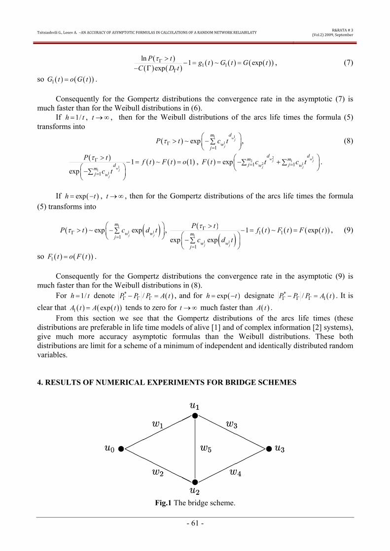
Consider the no oriented graph Γwith the final nodes set U the arcs set W the fixed initial and final nodes u v and the set of the acyclic ways 1 nRR between u v Suppose that the probability
wp of the arc Wwisin work depends on the parameter h gt 0 )(hpp ww = and 0)( rarrhpw 0rarrh Denote )( pUP - the probability of the event pU that all arcs p
mp
pww 1 of the way pR work Then
the reliability of the port Γ is 1
⎟⎟⎠
⎞⎜⎜⎝
⎛=
=Γ U
n
ppUPP denote
1( )
n
pp
P P UΓ=
=sum
Remark that for qp ne the arcs sets pRwisin qRwisin can not satisfy the inclusion qp RwRw isinsubeisin In an opposite case there is the node u in which the ways pR qR diverge by
the arcs )( puu )( quu But as the arc )( qp Rwuu isinisin so there is a circle in the way qR This statement contradicts with a suggestion that the way qR is acyclic As the inclusion
qp RwRw isinsubeisin is not true for qp ne so the way pR contains the arc qRwnotin and consequently ))(()( pqp UPoUUP = 0rarrh qp ne An induction by n gives the inequality
)(
1
ΓΓ
leltleΓ leleminus sum PPUUPP
nqpqp (1)
But
1
)(max)( Γisin
leltle
lesum PhpnUUP wWwnqpqp
Tsisiashvili G Losev A ndash AN ASYMPTOTIC ANALYSIS OF A RELIABILITY OF INTERNET TYPE NETWORKS
RampRATA 3
(Vol2) 2009 September
- 26 -
and consequently from the formula (1) we obtain
~ ΓΓ PP (2)
Denote by A = |1| minusΓΓ PP the relative error of the asymptotic formula (2) It is obvious that
00)()(max)( rarrrarr=le
isinhhФhpnhA wWw
(3)
Assume that 0)( rarrhϕ 0rarrh then for the replacement of h by )(hϕ the upper bound )(hФ of
the relative error is to be replaced by ))(())(( hФohФ =ϕ Radial-circle scheme Consider the radial-circle scheme represented on the fig 1 This
scheme has the center 0 connected with the nodes 1hellipn arranged on the circle
Fig1 Radial-circle scheme
Each acyclic way from the node i 1 ni lele on the circle (the circle node) to the center 0 of
this scheme consists of a peace along the circle and a transition to the center 0 A way from the circle node i to the circle node j 1 nji lenele has a peace from the node i along the circle a transition to the center 0 a transition to the circle and a peace along the circle to the node j
Define the connection matrix P njiijP 0|||| == of the radial-circle scheme in which ijP is the
probability that there is a working way between the nodes i j of this scheme Represent the results of the matrix P calculation with n=6 and
Remark Analogously it is possible to obtain asymptotic formulas for a general type network
or a radial circle scheme with high reliable arcs But in this case it is necessary to replace a work probability by a failure probability and a way by a cross section
2 Recursively defined networks A calculation of the connection matrix in recursively defined networks Suppose that D
is the set of networks Γ with no intersected sets of arcs Define recursively the networks class DDD sub by the condition
Ш 21222111 =capisin=Γisin=Γ WWDWUDWU (4) node) single a is (z 2121 DzUU isinΓcupΓrarr=cap
Analogously to [2] in this paper we calculate vuUvuP neisinΓ not its single element
These calculations are based on the recursive formulas if zUUDD =primeprimecapprimeisinΓ primeprimeisinΓprime then
⎪⎩
⎪⎨
⎧
primeprimeisinprimeisin
primeprimeisin
primeisin=
Γ primeprimeΓprime
Γ primeprime
Γprime
Γ primeprimecupΓprime
UvUuPPUvuPUvuP
P (5)
Tsisiashvili G Losev A ndash AN ASYMPTOTIC ANALYSIS OF A RELIABILITY OF INTERNET TYPE NETWORKS
RampRATA 3
(Vol2) 2009 September
- 28 -
In the last equality the quantity ΓprimeP characterizes the connection between the nodes u z and
the quantity Γ primeprimeP ndash the connection between the nodes z v The number of arithmetical operations )( ΓPn necessary to calculate vuUvuP neisinΓ by the recursive formulas (5) is characterized by
the following statement
Theorem Suppose that lΓΓ 1 is the sequence of networks with the no intersected sets of arcs If D consists of sequences of independent probability copies of 1 lΓΓ then for each DisinΓ the
inequalities
1
( )( ( ) 1) ( )( ( ) 1)( ) ( )2 2 i
i
l
u v U u v i u v U u v
l l l ln P n PΓ Γisin ne = isin ne
Γ Γ minus Γ Γ minusle le +sum sum sum (6)
are true with l )(Γ the number of nodes in the graph Γ
From the inequalities (6) obtain that
1)1)()((
)(2lim
)(=
minusΓΓ
sumneisin
Γ
infinrarrΓ ll
PnvuUvu
l
So asymptotically when infinrarrΓ)(l to calculate a connection probability for a single pair of
nodes it is necessary a single arithmetical operation Proof Suppose that the inequality (6) is true for Γprime then from the recursive formulas (5) and
the equality 1)()()( minusΓprimeprime+Γprime=Γ primeprimecupΓprime lll we have
+minusΓΓ
+minusΓΓ
+lesum sumsum= neisin
Γneprimeprimecupprimeisin
Γ primeprimecupΓprime 2)1)()((
2)1)()(()()( 2211
1
llllPnPnl
i vuUvuvuUUvu i
i
2
)1)()(()()1)()(1)(( 2121
1 21
minusΓcupΓΓcupΓ+=minusΓminusΓ+ sum sum
= neisinΓ
llPnlll
i vuUvu i
i
A calculation of the transition matrices in the internet type networks Analogously to [1]
define the class of the internet type networks as the recursively defined class of networks D with the set of originating schemes D which consists of radial-circle schemes and in the formula (4) the node z is the center of the radial-circle scheme 2Γ
Tsisiashvili G Losev A ndash AN ASYMPTOTIC ANALYSIS OF A RELIABILITY OF INTERNET TYPE NETWORKS
RampRATA 3
(Vol2) 2009 September
- 29 -
Fig2 The internet type network
So if we have the transition matrix for the radial-circle schemes it is possible to calculate the transition matrix of the internet type network by the formula (5) This algorithm is significantly faster than general type algorithm from [1] It contains fast algorithm to calculate the transition matrix in the radial-circle scheme and practically optimal algorithm to calculate the transition matrix for the internet type networks
REFERENCES
1 Ball M O Colbourn C J and Provan J S Network Reliability In Network Models Handbook of Operations Research and Management Science 1995 Elsevier Amsterdam Vol 7 P 673-762
2 Floid RW Steinberg L An adaptive algorithm for spatial greyscale SID 75 Digest 1975 Pp 36-37
Salem Bahri Fethi Ghribi Habib Ben Bacha ndash A STUDY OF ASYMPTOTIC AVAILABILITY MODELING FOR A FAILURE AND A REPAIR RATES FOLLOWING A WEIBULL DISTRIBUTION
RampRATA 3
(Vol2) 2009 September
- 30 -
A STUDY OF ASYMPTOTIC AVAILABILITY MODELING FOR A FAILURE AND A REPAIR RATES FOLLOWING A WEIBULL
DISTRIBUTION
Salem Bahri a Fethi Ghribi b Habib Ben Bacha ac
a Electro Mechanical systems laboratory (LASEM) Department of Mechanical Engineering-ENIS
e-mail SalemBenBahrienisrnutn b Department of Mathematical and Computer Science National Engineering School
of Sfax (ENIS) University of Sfax BP W Sfax 3038 Tunisia e-mail fethighribienisrnutn
c King Saud University- College of Engineering in Alkharj-PO Box 655 Elkharj11942 Kingdom of Saudi Arabia
e-mail hbachaksuedusa Abstract
The overall objective of the maintenance process is to increase the profitability of the
operation and optimize the availability However the availability of a system is described according to lifetime and downtime It is often assumed that these durations follow the exponential distribution The work presented in this paper deals with the problem of availability modeling when the failure and repair rates are variable The lifetime and downtime were both governed by models of Weibull (the exponential model is a particular case) The differential equation of the availability was formulated and solved to determine the availability function An analytical model of the asymptotic availability was established as a theorem and proved As results deduced from this study a new approach of modeling of the asymptotic availability was presented The developed model allowed an easy evaluation of the asymptotic availability The existence of three states of availability for a system has been confirmed by this evaluation Finally these states can be estimated by comparing the shape parameters of the Weibull model for the failure and repair rates Keywords Availability function asymptotic availability failure rate repair rate Weibull distribution 1 Introduction
The last two decades witnessed major progress in the development of new maintenance strategies [1] The primary objectives of these strategies are to reduce equipment downtime also increase reliability and availability of the equipment which at the same time optimizes the life-cycle costs [2] The need for high reliability and availability is not just restricted to safety-critical systems [3] In general current technology has ensured that the equipments for industrial application for example telephone switches airline reservation systems process and production control stock trading system computerized banking etc all require very high availability [2] Reliability is generally described in terms of the failure rate or mean time between failures (MTBF) while availability is normally associated with total downtime [2] There is some research on increasing system availability [4] Goel and Soenjoto proposed a generalized model [4] Markov models are also implemented to analyze the system availability which combines both software and hardware failures and maintenance processes [4] Khan and Haddara [1] proposed a methodology for risk-based maintenance to increase availability of a heating ventilation and air-conditioning (HVAC) system Garg S et al [3] developed a model for a transactions based software system which
Salem Bahri Fethi Ghribi Habib Ben Bacha ndash A STUDY OF ASYMPTOTIC AVAILABILITY MODELING FOR A FAILURE AND A REPAIR RATES FOLLOWING A WEIBULL DISTRIBUTION
RampRATA 3
(Vol2) 2009 September
- 31 -
employs preventive maintenance to maximize availability minimize probability of loss minimize response time or optimize a combined measure The steady state availability can be modelled using standard formulae from Markov regenerative process (MRGP) theory The Service rate and failure rate are assumed to be functions of real time (Weibull distribution) [3] The failure and repair rates are supposed constant (λ and μ respectively) so that system availability can be modeled using a Markov chain in Refs [57] But Khan and Haddara [1] considered that the Weibull model is more robust than the other models Dai et al [4] studied the availability of the centralized heterogeneous distributed system (CHDS) and developed a general model for the analysis The repair time was exponentially distributed For the failure intensity function (failure rate) the GO model presented by Goel and Okumoto was used [4] Some other research considered that the availability depends on both reliability and maintainability and is defined as the ratio of requested service time to practical service time [6 7]
Nomenclature A(t) Availability function Ainfin Asymptotic availability λ(t) Failure rate μ(t) Repair rate β Shape parameter of Weibull distribution for Failure rate η Scale parameter of Weibull distribution for Failure rate α Shape parameter of Weibull distribution for repair rate θ Scale parameter of Weibull distribution for repair rate
Review of the literature indicates that there is a new trend to use availability and reliability
modeling as a criterion to plan maintenance tasks However most of the previous studies assumed the failure andor repair rates are constant It seems that there is a need for a more generalized methodology that can be applied for variable rates The present study adopts a new fundamental approach for the asymptotic availability modeling where the failure and repair rates were governed by the Weibull distribution This paper is organized as follows In Section 2 the differential equation of the availability is established Section 3 is dedicated to the resolution of the differential equation to determine the instantaneous availability The model of the asymptotic availability is developed in Section 4 Finally in Section 5 the conclusions along with future research directions are presented 2 The mathematical formulation of the availability differential equation
According to the standard ldquoAssociation Franccedilaise de Normalisation - AFNOR X 06-503rdquo [8
9] in order to have a system available at time t+dt there are two possibilities bull the first is that the system is available at time t and does not have breakdown between t
and t+dt bull the second is the system is unavailable at time t but it is repaired between t and t+d These expressions are transformed by the following probabilities
A(t+dt) The probability that the system is available at time (t+dt) A(t) the probability that the system is available at time t 1-(t)dt The probability that the system does not have breakdown between t and t+dt
knowing that it had already functioned until the time t 1-A(t) The probability that the system is unavailable at time t
Salem Bahri Fethi Ghribi Habib Ben Bacha ndash A STUDY OF ASYMPTOTIC AVAILABILITY MODELING FOR A FAILURE AND A REPAIR RATES FOLLOWING A WEIBULL DISTRIBUTION
RampRATA 3
(Vol2) 2009 September
- 32 -
(t)dt The probability that the system is repaired between t and (t+dt) knowing that it was already failing until the time t
A(t+dt)= probabilities (that the system is up at t and is no break down between t and
(t+dt))+ probabilities (the system to be down at time t and it is repaired between t and (t+dt)) [8 9]
(1) (2)
(3) Then
(4)
This expression represents the differential equation of first order of the availability [48 9]
3 The availability function
For t gt 0 the failure and repair rates which are modeled using a Weibull distribution are given by
- (5)
- (6) - Eq (4) can be solved by ldquoMathematica softwarerdquo by taking account of the initial
conditions A(0)=0 if the system is in the failure state and A(0)=1 if the system is in the functioning state and can be obtained the following solutions
bull If A(0) = 0 then
(7)
bull If A(0) = 1 then
Salem Bahri Fethi Ghribi Habib Ben Bacha ndash A STUDY OF ASYMPTOTIC AVAILABILITY MODELING FOR A FAILURE AND A REPAIR RATES FOLLOWING A WEIBULL DISTRIBUTION
RampRATA 3
(Vol2) 2009 September
- 33 -
(8)
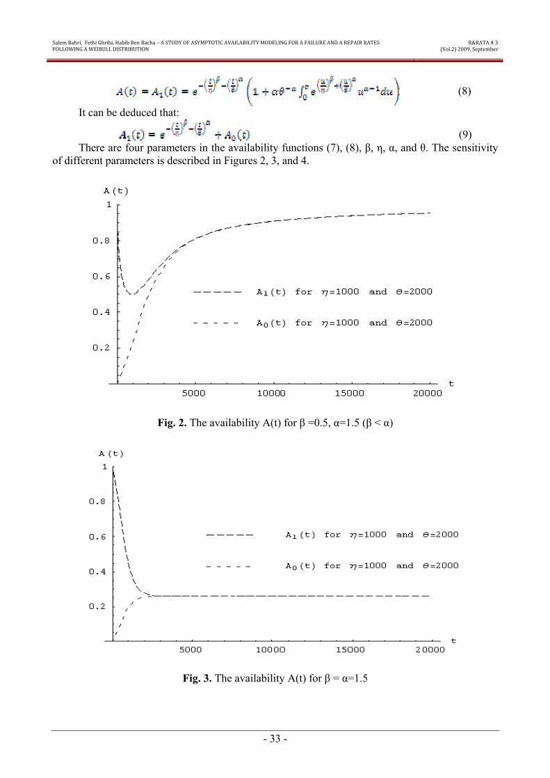
It can be deduced that
(9) There are four parameters in the availability functions (7) (8) β η α and θ The sensitivity
of different parameters is described in Figures 2 3 and 4
Fig 2 The availability A(t) for β =05 α=15 (β lt α)
Fig 3 The availability A(t) for β = α=15
Salem Bahri Fethi Ghribi Habib Ben Bacha ndash A STUDY OF ASYMPTOTIC AVAILABILITY MODELING FOR A FAILURE AND A REPAIR RATES FOLLOWING A WEIBULL DISTRIBUTION
RampRATA 3
(Vol2) 2009 September
- 34 -
Fig 4 The availability A(t) for β =15 α= 05 (β gt α)
4 The Asymptotic availability 41 Theorem
(10)
Demonstration It can be assumed that
(11)
Where if A(t)=A0(t) (12)
And if A(t)=A1(t) (13)
It may be necessary to prove that (14)
There are four intermediate results can be used to explain this 1st result
(15) Proof From Eq (12) this can be obtained by substituting A1(t) by Eq(9)
(16)
An analogy with Eq (9) can be deduced
(17)
Therefore from Eq (17) it is necessary to verify the 1st result to prove
(18)
(19)
Salem Bahri Fethi Ghribi Habib Ben Bacha ndash A STUDY OF ASYMPTOTIC AVAILABILITY MODELING FOR A FAILURE AND A REPAIR RATES FOLLOWING A WEIBULL DISTRIBUTION
RampRATA 3
(Vol2) 2009 September
- 35 -
Referring to Eqs (5) and (6)
(20)
Then Eq (19) will become
(21)
The limit study of Eq 18 gives
Figure 1 (22) And
(23)
So and the 1st result is verified 2nd result
(24)
Proof From Eqs 16 and 17 the function is written as
(25)
According to Eqs (7) and (20) The Eq (25) will become as follow
(26)
A change of variables is applied in Eq (26)
(27)
(28)
Therefore and the 2nd Result is
verified 3rd result
According to the shape parameters β and α the r0(t) function should satisfy the two following inequalities a) If βle α then
(29)
Or b) If βge α then
(30)
Proof a) For βle α
(31)
Salem Bahri Fethi Ghribi Habib Ben Bacha ndash A STUDY OF ASYMPTOTIC AVAILABILITY MODELING FOR A FAILURE AND A REPAIR RATES FOLLOWING A WEIBULL DISTRIBUTION
RampRATA 3
(Vol2) 2009 September
- 36 -
And (32)
By referring to the second result (24) and the two above mentioned inequalities (31) and (32) so the function can be put under the form of the following inequality
(33) The calculations of exponential integral allow to express the inequality (33) as follow
(34)
(35)
So the first inequality (29) is
satisfied b) For βge α
A similar development and demonstration is used for this case also
(36)
And
(37)
According to the second result (24) and the two above mentioned inequalities (36) and (37) so the r0(t) function can be put under the form of the following inequality
(38) The calculations of exponential integral allow to express the inequality (38) as follow
(39)
(40)
(41)
Salem Bahri Fethi Ghribi Habib Ben Bacha ndash A STUDY OF ASYMPTOTIC AVAILABILITY MODELING FOR A FAILURE AND A REPAIR RATES FOLLOWING A WEIBULL DISTRIBUTION
RampRATA 3
(Vol2) 2009 September
- 37 -
So the second inequality (30) is
satisfied 4th result
(42) Proof a) βle α By referring to the third result inequality (29) to prove the fourth result it can be sufficient to show that the limits
(43)
And
(44)
Then
(45)
(46) And
(47)
So if βle α b) β ge α In the same way as explained in the previous case according to inequality (30) to prove the fourth result it can be sufficient to show that the limits
(48)
And
(49)
Then
(50)
And
(51)
(52)
Salem Bahri Fethi Ghribi Habib Ben Bacha ndash A STUDY OF ASYMPTOTIC AVAILABILITY MODELING FOR A FAILURE AND A REPAIR RATES FOLLOWING A WEIBULL DISTRIBUTION
RampRATA 3
(Vol2) 2009 September
- 38 -
So and the 4th result (42) is proven also for αle β Finally the theorem (10) ensues therefore of results 1 and 4 The availability A(t) is plotted together with The function in figure 5 for βltα figure 6 for
β=α and figure 7 for βgtα The three figures show that the availability A(t) with its two solution A0(t) and A1(t) and the
function have tendency to converge towards the same limit when the time t is more
important
Fig5 The availability A(t) and ( )
( ) ( )μ t
μ t +λ t for β =05 α=15 (β lt α)
Fig6 The availability A(t) and ( )
( ) ( )μ t
μ t +λ t for A(t) for β = α=15
Salem Bahri Fethi Ghribi Habib Ben Bacha ndash A STUDY OF ASYMPTOTIC AVAILABILITY MODELING FOR A FAILURE AND A REPAIR RATES FOLLOWING A WEIBULL DISTRIBUTION
RampRATA 3
(Vol2) 2009 September
- 39 -
Fig7 The availability A(t) and ( )
( ) ( )μ t
μ t +λ t for A(t) for β =15 α=05 (β gt α)
42 Asymptotic availability evaluation According to (10) the asymptotic availability is defined by
(53)
(54)
The study of the limit of the function will be done according to three following cases 1st case βltα
(55)
Then (56)
The converge of the function when the time t is more important to the Ainfin= 1 with the
sensitivity of the scale parameters (ηltθ η=θ or ηgtθ) is shown in Fig8
Fig8 The ( )
( ) ( )μ t
μ t +λ t function limit studies for β=05 α=15 (β lt α)
2nd case β=α
Salem Bahri Fethi Ghribi Habib Ben Bacha ndash A STUDY OF ASYMPTOTIC AVAILABILITY MODELING FOR A FAILURE AND A REPAIR RATES FOLLOWING A WEIBULL DISTRIBUTION
RampRATA 3
(Vol2) 2009 September
- 40 -
(57)
In this case the asymptotic availability is defined to be equal to (58)
Particular cases β=α=1 the exponential models
(59)
With and
if η=θ then (60)
Fig 9 shows the asymptotic availability plotted with = with the sensitivity of the scale parameters (ηltθ η=θ or ηgtθ)
Fig9 The function ( )
( ) ( )μ t
μ t +λ t if β= α=1
3rd case βgtα
(61)
(62)
The converge of the function when the time t is more important to the Ainfin= 0 with the
sensitivity of the scale parameters (ηltθ η=θ or ηgtθ) is shown in Fig10
Salem Bahri Fethi Ghribi Habib Ben Bacha ndash A STUDY OF ASYMPTOTIC AVAILABILITY MODELING FOR A FAILURE AND A REPAIR RATES FOLLOWING A WEIBULL DISTRIBUTION
RampRATA 3
(Vol2) 2009 September
- 41 -
Fig10 The ( )
( ) ( )μ t
μ t +λ t function limit studies for β=15 α=05 (βgtα)
5 Conclusion
In this paper the presented work extended the classic availability model to a new asymptotic availability model when the failure and repair rates are distributed according to the Weibull model The analysis of asymptotic behavior of the system according to the developed model allowed to extract the following result
The asymptotic availability depends only on the shape parameters of the Weibull models β
and α The scale parameters η and θ do not have an influence in the limit of the availability
- If b alt then the system is fully available - If b agt the system resides in the down state then it is unavailable - If b a= in this case the asymptotic behavior of the system is analogous to a system governed by the exponential model
Thus the future plan includes the research on a novel approach which will be the
combination of two different models (Weibull Gamma) or (Weibull lognormal)
REFERENCES 1 Khan FI Haddara M M Risk-based maintenance (RBM) a quantitative approach for
maintenanceinspection scheduling and planning Journal of Loss Prevention in the Process Industries 200316 561ndash573
2 Ogaji SOT Singh R Advanced engine diagnostics using artificial neural networks Applied Soft Computing 20033 259ndash271
3 Garg S Puliafito A Telek M Trivedi K S Analysis of Preventive Maintenance in Transactions Based Software Systems IEEE Trans Comput 1998 471 96ndash107 (special issue on dependability of computing systems)
Salem Bahri Fethi Ghribi Habib Ben Bacha ndash A STUDY OF ASYMPTOTIC AVAILABILITY MODELING FOR A FAILURE AND A REPAIR RATES FOLLOWING A WEIBULL DISTRIBUTION
RampRATA 3
(Vol2) 2009 September
- 42 -
4 Dai YS Xie M Poh KL Liu GQ A study of service reliability and availability for distributed systems Reliab Engng Syst Safety 2003 79 103ndash112
5 Volovoi V Modeling of system reliability Petri nets with aging tokens Reliab Engng Syst Safety 200484149ndash161
6 Tsai YT Wang KS Tsai L C A study of availability-centred preventive maintenance for multi-component systems Reliab Engng Syst Safety 2004 84 261ndash270
7 Ji1 M Yu1 SH Availability Modeling for Reliable Routing Software Proceedings of the 2005 Ninth IEEE International Symposium on Distributed Simulation and Real-Time Applications (DS-RTrsquo05) IEEE Computer Society 2005
8 AFNOR Recueil des normes franccedilaise maintenance industrielle AFNOR Paris 1988 p 436-573
9 Monchy F Maintenance meacutethodes et organisations Paris eacutedition Dunod 2000 p 137-233
Igor Ushakov Sumantra Chakravarty ndash OBJECT ORIENTED COMMONALITIES IN UNIVERSAL GENERATING FUNCTION FOR RELIABILITY AND IN C++
RampRATA 3
(Vol2) 2009 September
- 43 -
OBJECT ORIENTED COMMONALITIES IN UNIVERSAL GENERATING FUNCTION FOR RELIABILITY AND IN C++
Igor Ushakov5
Sumantra Chakravarty6
Abstract
The main idea of Universal Generating Function is exposed in reliability applications Some commonalities in this approach and the C++ language are discussed Keywords Universal Generating function (UGF) C++ reliability INTRODUCTION
Usually binary systems are considered in the reliability theory However this approach does not describe systems with several levels of performance sufficiently Analysis of multi-state systems forms now a special branch of the reliability theory
For analysis of such systems consisting of multi-state subsystemselements one can use the method of Universal Generating Functions (UGF) which is described below 1 GENERATING FUNCTION
One frequently uses an effective tool in probabilistic combinatorial analysis the method of generating functions For a distribution function of a discrete random variable ξ such that kpk ==ξPr for any natural k the generating function has the form
sum=k
kk xpx)(ϕ
Advantages of using a generating function are well established in this field and we list a few of those
(1) For many discrete distributions (eg binomial geometrical Poisson) there are compact forms of generating functions which allows one to get analytical solutions quickly and easily
(2) Moments of statistical distributions can be written in convenient forms For example the mathematical expectation of random variable ξ can be found as
1
)(=part
part=
x
xx
E ϕξ
(3) If there are n independent random variables 1ξ 2ξ nξ with the respective generating functions )(1 xϕ )(2 xϕ )(xnϕ then the following generation function can be written for the convolution of these distributions
5 igorushakovgmailcom 6 sumontrohotmailcom
Igor Ushakov Sumantra Chakravarty ndash OBJECT ORIENTED COMMONALITIES IN UNIVERSAL GENERATING FUNCTION FOR RELIABILITY AND IN C++
RampRATA 3
(Vol2) 2009 September
- 44 -
prod=
=n
jj xx
1
)()( ϕϕ
where sum=k
kjkj xpx)(ϕ and pjk is the probability that j-th random variable takes value k
2 COMPUTER ALORITHM FOR CALCULATION PRODUCT OF GFrsquoS
Let us present a generating function as a set of objects Each object corresponds to a term in the generating function polynomial It means that object is a pair of two values the first is the coefficient ie probability p and the second is the power of the argument a ie the corresponding random variable
Consider a computational algorithm for calculation of the convolution of two distributions One makes the following formal operations
diams Take two sets of objects set )( 1111 ap )( 1212 ap )( 11 kk ap for generating function )(1 xϕ and set
)( 2121 ap )( 2222 ap )( 22 mm ap for generating function )(2 xϕ
diams Find all cross ldquointeractionsrdquo of objects of the first set with all objects of the second set using the following rule
[Interacting objects )( 11 kk ap and )( 22 mm ap ] [Resulting object )( 2121 mkmk aapp + ] diams For all resulting objects with different
11ka for object-1 and 22ma for object-2 but such
that 11ka +
22ma =a one forms a new final resulting object )(21 21 app mksum The total set of
such final resulting objects gives us the needed solution from here we can get probabilities for any a
3 UNIVERSAL GENERATING FUNCTION
We have described a formalized procedure on sets of objects interaction coresponding to product of polynomials But in practice we meet a number of situations when this operation is not enough Consider the following simple examples
Example 1 Assume that there is a series connection of two (statistically independent)
capacitors (Fig 1)
Fig 1 Series connection of two capacitors
Igor Ushakov Sumantra Chakravarty ndash OBJECT ORIENTED COMMONALITIES IN UNIVERSAL GENERATING FUNCTION FOR RELIABILITY AND IN C++
RampRATA 3
(Vol2) 2009 September
- 45 -
Assume that c1 and c2 are random with discrete distributions p1k=Prc1=k and p2j=Prc2=j One is interested in distribution of total capacity It is impossible to find the solution with the help of a common generating function However there is a possibility to use formal algorithm described above with the use of corresponding operations over the elements of the objects The following procedure can be suggested
diamsTake two sets of objects S1 and S2 S1 = )( 1111 cp )( 1212 cp )( 11 kk cp
and S2 = )( 1121 cp )( 2222 cp )( 22 mm cp
where k is the number of discrete values of the first capacitor and m is the same for the second one Here the first element of the object is the probability and the second element is the respective capacity
diamsFind all cross ldquointeractionsrdquo Ω of objects of set S1 with all objects of set S2 using the following rule
Ω )( 11 ii cp )( 22 jj cp = )( ijij cp
Here ijp is the resulting probability calculated in accordance with the multiplication rule
(under assumption of independence) as jijipij ppppp 2121)(
=Ω= where )( pΩ is the rule of interaction of parameters p which in this particular case is multiplication Value of
ijc is the resulting capacity calculated in accordance with the harmonic sum rule for capacities
( ) 112
1121)(
minusminusminus +=Ω= jijicij ccccc where )(cΩ is the rule of interaction of parameters c
diams Assume that in result we obtain all R=km possible resulting objects of kind )( cp Let
us order all these resulting pairs in increase of value of c )( 1
1 cp )(
RR cp For some resulting pairs with numbers say i i+1hellip i+j values of c can be the same and equal some C We converge such objects into a single aggregated object with parameters )( Cp
jisissum
+lele
The total set of such final resulting objects gives us the needed solution
The procedure can be easily expanded on a series connection of several independent capacitors
nrjinrjiSER
p pppppp sdotsdotsdot=Ω 2121)( аnd
[ ] 1112
1121)(
minusminusminusminus +++=Ω nrjinrjiSERc cccccc
Example 2 Pipeline consists of n series sections (pipes) Section j is characterized by random capacity for which each value v is realized with some probability p In this case
nrjinrjiPARp pppppp sdotsdotsdot=Ω 2121)(
аnd
Igor Ushakov Sumantra Chakravarty ndash OBJECT ORIENTED COMMONALITIES IN UNIVERSAL GENERATING FUNCTION FOR RELIABILITY AND IN C++
RampRATA 3
(Vol2) 2009 September
- 46 -
nrjinrji
SERc vvvvvv min 2121)( =Ω
Example 3 One measures a sum of values each summand of which is random With
probability jsp value j is measured with standard deviation (STD) equal to jsσ In this case using notation similar to above one has
nrjinrji
PARp pppppp sdotsdotsdot=Ω 2121)(
аnd 22
22121)( nrjinkjic n
σσσσσσ +++=Ω
Examples can be continued and not necessarily with probabilistic parameters 4 FORMAL DESCRIPTION OF THE METHOD OF UNIVERSAL GENERATING
FUNCTIONS
After these simple examples let us begin with formal description of the Method of Universal Generating Function (UGF7) For a more vivid presentation let us use special terminology to distinguish the UGF from the common generation function This will relieve us from using traditional terms in a new sense which may lead to some confusion Moreover we hope that this new terminology can help us in a mnemonic sense to remember and perhaps even to explain some operations
In the ancient Roman army a cohort (C) was the main combat unit Each cohort consisted of maniples (M) which were independent and sometimes specialized combat units with several soldiers of different profiles Several cohorts composed a legion (L) The use of this essentially military terminology appears to be convenient in this essentially peaceful mathematical application A legion is close by its sense to a generating function a cohort is close to a term of the generating function written in the form of expanded polynomial and a maniple is close to a parameter of each term
Starting with polynomial multiplication in our approach we will consider less restrictive operations (not only multiplication of terms) and more general parameters For instance multiplication of polynomials assumes getting products of coefficients and summation of powers In our case we will expand on such restrictive limits on operations
Letrsquos denote legion j by Lj This legion includes vj different cohorts Cjk
( )jjvjjj CCCL 21=
The number of cohorts within different legions might be different However in our approach
maniples which consist of a cohort must be similar by its structure Each cohort jkC is composed of some maniples M each of which represents different
parameters special characteristics and auxiliary attributes Each cohort consists of the same set of maniples
( ))()2()1( sjkjkjkjk MMMC =
7 UGF might be also read as Ushakovrsquos Generating Function
Igor Ushakov Sumantra Chakravarty ndash OBJECT ORIENTED COMMONALITIES IN UNIVERSAL GENERATING FUNCTION FOR RELIABILITY AND IN C++
RampRATA 3
(Vol2) 2009 September
- 47 -
To make description of the method more transparent let us start with the examples of two
legions L1 and L2 each of which consists of the following cohorts L1=(C12C12C13) and L2=(C21C22) and each cohort Cjk includes two maniples )1(
jkM and )2(jkM ie Cjk=( )1(
jkM )2(jkM )
Denote the operation of legion interaction by LΩ This operator is used to obtain the resulting legion LRES In this simple case one can write
21 LLL LRES Ω= (1)
This interaction of legions produces six pairs of interactions between different cohorts which generate the following resulting cohorts
21111 CCC CRES Ω=minus 22112 CCC CRES Ω=minus
21123 CCC CRES Ω=minus 22124 CCC CRES Ω=minus
21135 CCC CRES Ω=minus 22136 CCC CRES Ω=minus
Here bullΩC denotes the interaction of cohorts
Interaction of cohorts consists of interaction between its costituent maniples All cohorts contain maniples of the same types though with individual values of parameters Let us take for instance resulting cohort CRES-5 which is obtained as interaction of cohorts C13 and C21 In turn interaction of these particular cohorts consists in interaction of their corresponding maniples
)1(
21)1(
13)1(
5 )1( MMMMRES Ω=minus
)2(21
)2(13
)2(5 )2( MMM
MRES Ω=minus
The rules of interaction between maniples of different types ie )1(2
)1(1 )1(
ji MMMΩ and
)2(2
)2(1 )2(
ji MMMΩ are (or might be) different
Interaction of n legions can be written as
) 21( nLLLLL Ω=
Operator LΩ denotes a kind of ldquon-dimensional Cartesian productrdquo of legions and special final ldquoreformattingrdquo of the resulting cohorts (like converging polynomial terms with the equal power for a common generating function) Since each legion j consists of vj cohort the total number of resulting cohorts in the final legion (after all legion interaction) is equal to
prodlele
=nj
jvv1
Number v corresponds to the total number of cohortsrsquo interactions
Igor Ushakov Sumantra Chakravarty ndash OBJECT ORIENTED COMMONALITIES IN UNIVERSAL GENERATING FUNCTION FOR RELIABILITY AND IN C++
RampRATA 3
(Vol2) 2009 September
- 48 -
5 IMPLEMENTING UGF PHILOSOPHY IN COMPUTER LANGUAGE C++
We would like use the UGF (Universal Generating Function) philosophy in an analysis tool and perform reliability calculations for real-world systems Because we are talking about an (reliability) engineering discipline all philosophies present the need to be converted into numerical results and predictions Thus the UGF philosophy begs an implementation The implementation task is to identify objects (maniple cohort legion) and program all interactions between them Unfortunately we run into a combinatoric explosion of possible interactions for a sysem consisting of a large number of (atomic) units Even moderm computers are not able to enumerate astronomically large (21000) number of interaction states in system consisting of 1000 binary atomic units Fortunately for a class of frequently occuring practical systems the situation is not as hopeless as it may first appear For a system to be useful in engineering it may only fail very infrequently In a highly reliable system the failure probability of all atomic units much smaller that the system failure probability This fact makes most of the interactions exceedingly rare and they can be systematically ignored in an approximation scheme that retains only the dominant contributions
Let us proceed to find an approximate implementation of the UGF philosophy for highly relaible systems in a system simulator It should be reasonably easy to identify an atomic unit in reliability theory as a maniple Independence of the maniples corresponds to statistical independence of the atomic units A cohort is defined to be a collection of maniples The same definition holds in the context of reliability theory where the collection is defined by a failure criterion In a series system each atomic unit is assumed to provide distinct and critical functionality This maps on to the notion of specialized combat units In a parallel system all atomic units are statistically identical This improves survival probability during operation either in the military or in system reliability Thus we may identify a subsystem in reliability engineering as a cohort in UGF formalism
Interactions between the objects are identified in the simulator by their natural reliability names k-out-of-n combinations are of primary interest But this class includes the two most frequently appearing reliability structures series (n-out-of-n) and parallel (1-out-of-n) In fact probability of failure of a parallel system is negligible (higher order in numerical smallness) with an additional assumption of high availability of the atomic units Obviously a series system can be made up of distinct units providing separate functionality to the system
As an illustration let us consider a system S of two subsystems A and B in series Let A be atomic and B be composed of two atomic units X and Y in parallel One possible C++ coding for this (simple) system is
B=Parallel(XY) S = Series(AB)
Properties (MTBF MTTR etc) of all atomic units are specified at the start of analysis Operations like Series and Parallel are C++ member functions for the instances of class ldquounitrdquo We will not specify unit composition rules in this work Most of these rules can be found in standard textbooks on reliability engineering Interested readers may find the remaining ones (involving switching time and PEI) in Chakravarty and Ushakov (2000 2002)
It remains to identify the ldquolegionrdquo The preceding paragraphs almost suggest that a legion be identified with the entire system in reliability theory where the system is further assumed to be represented by its generating function We would like to note that that this analogy cannot be taken literally sometimes It is common for a real world reliability system to have deeper hierarchies (eg system equipment shelves equipment racks electornic cards) like modern day militaries In such an elaborate system we still identify the atomic units as maniples At the other end we identify the
Igor Ushakov Sumantra Chakravarty ndash OBJECT ORIENTED COMMONALITIES IN UNIVERSAL GENERATING FUNCTION FOR RELIABILITY AND IN C++
RampRATA 3
(Vol2) 2009 September
- 49 -
entire system as a ldquolegionrdquo All intermediate stages in the hierarchy are considered generalized ldquocohortsrdquo
In Chakravarty and Ushakov (2000) implementation any subsystem can be composed from other subsystems at the next lower level of hierarchy (or atomic units which are always at the lowest level) A newly formed subsystem provides an effective reliability description of all units that compose this subsystem This composition can be continued indefinitely to obtain an effectiveness measure for the entire system They have shown that this can be recast as an approximation from a system generating function when all atomic units satisfy binary failure criteria (onoff) they are statistically independent the system itself is highly reliable and reliability design of the system consists of hierarchical blocks 6 RELIABILITY ANALYSIS OF GLOBALSTARTM GATEWAYS
Globalstar is a low-earth-orbit (LEO) based telephony system with global coverage The gateways make its ground segment that connect to the orbiting satellites The gateways are cpmlex systems with more than a thousand components (eg electronic cards) Ushakov (1998) Chakravarty and Ushakov (2002) used the UGF approach for the reliability (performance) analysis of GlobalstarTM gateways (fixed ground segment of a low earth orbit satellite communications system) Given the prominence of object oriented abstractions and operations in Globalstar design it should not be surprising that the reliability analysis naturally fits into the UGF philosophy Further these ideas can be naturally implemented in the computer using an object oriented language
Because of the object oriented nature of system reliability design in Globalstar (interaction between objects like system racks shelves cards are triggered by failure switching of failed units and changing user demand) Ushakov (1998) proposed that a system reliability simulator should be coded in an object oriented computer language like C++ Later Chakravarty and Ushakov (2002) implemented a simulator for the GlobalstarTM Gateway in C++
In Chakravarty and Ushakov implementation for Globalstar C++ objects are in one-to-one correspondence with reliability objects An object is specified by mean time between failures (MTBF) mean time to repairreplace (MTTR) and an effectiveness weight (partial effectiveness index PEI) By definition PEI=1 for binary atomic units All failure distributions are implicitly assumed to be Exponential If failed units were to be automatically swapped a switching time was also assigned by Chakravarty and Ushakov (2000) Even small switching time is important because it changes a parallel system ldquoon paperrdquo to a series system with small MTTR This may have dramatic effect overall on system reliability
REFERENCES
1 Chakravarty S and Ushakov I Reliability measure based on average loss of capacity International Transactions in Operational Research Vol 9 No 2 2002
2 Chakravarty S and Ushakov I Effectiveness Analysis of GlobalstarTM Gateways Proceedings of Second International Conference on Mathematical Methods in Reliability (MMRrsquo2000) Vol 1 Bordeaux France 2000
3 Ushakov IA The Method of Generating Sequences European Journal of Operational Research Vol 1252 2000
4 Ushakov IA An object oriented approach to generalized generating function Proc of the ECCO-XI Conference (European Chapter on Combinatorial Optimization) Copenhagen May 1998
Igor Ushakov Sumantra Chakravarty ndash OBJECT ORIENTED COMMONALITIES IN UNIVERSAL GENERATING FUNCTION FOR RELIABILITY AND IN C++
RampRATA 3
(Vol2) 2009 September
- 50 -
5 Ushakov IA Reliability Analysis of Multi-State Systems by Means of a Modified Generating Function Journal of Information Processes and Cybernetics (Germany) Vol24 No3 1988
6 Gnedenko BV and IA Ushakov Probabilistic Reliability Engineering John Wiley amp Sons New York1995
7 Ushakov IA Solving of Optimal Redundancy Problem by Means of a Generalized Generating Function Journal of Information Processes and Cybernetics (Germany) Vol24 No4-51988
8 Ushakov IA Solution of Multi-Criteria Discrete Optimization Problems Using a Universal Generating Function Soviet Journal of Computer and System Sciences (USA) Vol 25 No 5 1987
9 Ushakov IA Optimal Standby Problem and a Universal Generating Function Soviet Journal of Computer and System Sciences (USA) Vol 25 No 4 1987
10 Ushakov IA A Universal Generating Function Soviet Journal of Computer and System Sciences (USA) Vol 24 No 5 1986
Alexandru Isaic‐Maniu Viorel Gh Voda ndash SOME INFERENCES ON THE RATIO AVERAGE LIFETIMETESTING TIME IN ACCEPTANCE SAMPLING PLANS FOR RELIABILITY INSPECTION
RampRATA 3
(Vol2) 2009 September
- 51 -
SOME INFERENCES ON THE RATIO AVERAGE LIFETIMETESTING TIME IN ACCEPTANCE SAMPLING PLANS FOR RELIABILITY
INSPECTION
Alexandru ISAIC-MANIU
Academy of Economic Sciences Bucharest Romania Faculty of Cybernetics Statistics and Economic Informatics
e-mail alisaic-maniucsieasero
Viorel Gh VODĂ
ldquoGh MIHOC - C IACOBrdquo Institute of Mathematical Statistics and Applied Mathematics of the Romanian Academy Bucharest
e-mail von_vodayahoocom
Abstract In this paper we construct effective single sampling plans for reliability inspection when the
distribution of failure times of underlying objects obey a Weibull law To this purpose we use the index average lifetime (E (T)testing time (T) for two values of E(T) - acceptable and non acceptable ones - and known shape parameter (K) of the Weibull cdf We derive also a relationship between this index and reliability function R(t) of the assumed statistical law A numerical illustrations is provided in the case of Rayleigh cdf - that is for a Weibull shape k = 2
Key words cdf - cumulative distribution function two-parameter Weibull law sampling plan average lifetime testing time Rayleigh case 1 Introduction From the SQC (Statistical Quality Control) perspective reliability is considered a dynamical quality characteristic since the performances of a given technical entity are put into light if the underlying element component or system is in a functional operational state performing a prescribed mission for a specified period of time Static quality characteristics (such as hardness length pressure volume aso) are observed and measured directly in units independent of time Metaphorically speaking reliability is viewed as one of the special features of the general concept of quality Vasiliu (1980 [7 page 26]) defines reliability as bdquothe dimension in time of qualityrdquo Two decades later Yang and Kapur (1997 [9 page 340]) state that bdquoreliability is quality over timerdquo Anyway no matter how good is a design how performing is the production process how careful is handled and exploited a technical system there is no way to stop its final decay After a certain period of time - which may be short or quite long - every human made object sooner or later will fail This event (failure) is due to natural causes (wear-out phenomenon) or to some bdquoartificialrdquo
Alexandru Isaic‐Maniu Viorel Gh Voda ndash SOME INFERENCES ON THE RATIO AVERAGE LIFETIMETESTING TIME IN ACCEPTANCE SAMPLING PLANS FOR RELIABILITY INSPECTION
RampRATA 3
(Vol2) 2009 September
- 52 -
ones as for instance the use of the item in inappropriate conditions (aggressive environment intensive operational tasks lack of adequate maintenance actions mishandling etc) A failure occurs in a random manner and usually after a certain period of time when the system was operating supposedly satisfactorily Since we do not know the exact moment when a specified object will fail we are forced to judge in terms of probabilities and averages involving the time elements as one of the main parameters The failure behavior of that specific object has to be modeled and hence we are facing to the problem of choosing the most suitable class of life distributions describing this time-to-failure phenomenon Nevertheless we may speak about the so-called bdquostatic reliabilityrdquo where the time element is not instantly (or explicitly) involved (see Blischke and Murthy 2000 [2 page 173 - 177]) We refer here to the so-called bdquostress-strength modelsrdquo where reliability is regarded as the capacity of itemrsquos strength (x) to resist to the action of stress (y) Actually a measure of reliability in this model is R = Prob x gt y where usually both x and y are random variables If this probability is greater than 50 we could expect a desirable reliability of the underlying entity In batch inspection procedures if the characteristic of interest is reliability (or durability) of underlying items we must take into account their failure behavior (where time element is the main parameter) in order to construct suitable sampling acceptance plans from economical point of view In this paper we shall present some new results on the index average lifetime (durability)testing time in the construction of acceptance sampling plans for reliability inspection when time-to-failure distribution is a two parameter Weibull one 2 Various approaches of reliability inspection It is well-known that a very general approach for batch inspection - no matter the nature of quality characteristic investigated - is that called attributive one All practical procedures have been already standardized - see the document MILSTD105 E bdquoSampling procedures and tables for inspection by attributesrdquo (see Kirkpatrick 1970 [5 page 354 - 415] where the variant D is entirely reproduced) The simplicity of attributive method lies in the fact that products are classified into categories conforming and defective (nonconforming) ones regarding some specified criteria In the case of reliabilitydurability inspection this attributive approach ignores the very nature of failure behavior of inspected objects and this could lead to a larger sample (or samples) to be tested if the items are quite expensive and since the specific test in this case is destructive the procedure appears to be non-economic It is important to notice that the attributive approach ignores in the case of reliabilitydurability inspection the following elements a) what kind of samples we use for inspection complete ones or censored ones b) distributional assumption for time-to-failure c) sampling is with replacement or non replacement d) testing conditions are normal or accelerated ones e) items are reparable or non-reparable (if they are non restoring then E(T) is just the mean durability and T (sample mean) is computed with ( ) ni1it lele values where ti is the time to first - and
Alexandru Isaic‐Maniu Viorel Gh Voda ndash SOME INFERENCES ON THE RATIO AVERAGE LIFETIMETESTING TIME IN ACCEPTANCE SAMPLING PLANS FOR RELIABILITY INSPECTION
RampRATA 3
(Vol2) 2009 September
- 53 -
last - failure of the ith item submitted to the test it is senseless to speak in this case about MTBF - Mean Time Between Failures) f) what is the relationship between testing time (T0) and the actual operating life of those items More useful are in such special case methods based on average operating time or on hazard rate associated to the failure time model specific for each peculiar instance The document MILSTD 781 Reliability test exponential distribution (US Dept of Defense Washington D C 1984) use the ratio E (T) T0 where E (T) is the average lifetime (durability) of underlying objects and T0 is the testing time In the exponential case ( ) ( ) 0θ0ttθexp1θtF gtgeminusminus= F being the cdf (cumulative distribution function) of the
representative variable (T) the mean-value of T is ( ) θTE = and therefore the inference is done straight forwardly on the distributional parameter (details are given in Cătuneanu-Mihalache 1989 [3] Vodă-Isaic Maniu [8]) We shall examine now this ratio E (T) T0 in the case of a Weibull distribution 3 The ratio E (T) T0 in the case of a Weibull distribution Let Tw be a two-parameter Weibull distribution with the following cdf
( ) ( ) 0kθ0tθtexp1kθtFT kw gtgeminusminus= (1)
The corresponding reliability function is ( )θtexpR kt minus= and the theoretical mean-value is
( ) ( )1k1ΓθTE 1k +sdot= where ( ) duu0
u1intinfin
minusminus=Γ ex x (2)
is the well-known Gamma function (see Isaic-Maniu 1983 [6 page 21]) We have hence
Therefore the ratio E(T)t depends on the shape parameter (k) of Weibullrsquos cdf and on its reliability function If we fix t = T0 and considering k to be known we have either to estimate R (T0) or to fix lower acceptable bound for it From (5) we can deduce
Alexandru Isaic‐Maniu Viorel Gh Voda ndash SOME INFERENCES ON THE RATIO AVERAGE LIFETIMETESTING TIME IN ACCEPTANCE SAMPLING PLANS FOR RELIABILITY INSPECTION
and taking into account a formula given in Abramowitz-Stegun (1979 [1 page 82]) namely
( ) ( )k
C11k1ln1k1Γln minus++minusasymp+ (8)
where C is the Euler-Mascheronirsquos constant ( )577210asymp If we approximate now ln (1+1k) as 1k (let us recall the inequalities ( ) ( ) )101ln1 1 ltlele+le+ minus xxxxx then if k gt 1 the relationship (7) becomes a very simple
estimation equation for the shape parameter if it is not known 4 Construction of acceptance sampling plans We shall start with the following assumptions (1) the items subjected to inspection are non-reparable (2) the failure time distribution is a two-parameter Weibull one with known shape parameter (3) we use only one sample with no replacement its size has to be determined (4) there is fixed an acceptable average lifetime [E(T)]1 corresponding to a given risk α (usually 050=α or 5) that is we wish to accept a lot with such average value with
9501 =minusα probability (5) there is fixed a non-acceptable average lifetime [E(T)]2 corresponding to a given risk β (usually 100=β or 10) that is we with to reject a lot with such average value with
9001 =minus β probability (6) there is fixed a testing time T0 smaller than the actual operating life of the underling items Therefore the sampling plan will be the system of objects (n A) | T0 where n and A are respectively the sample size and acceptance number which has to be determined and T0 is the previously fixed testing time The decision on the lot is taken as follows submit to the specific reliabilitydurability test a sample of size n drawn randomly from a lot of size N (n lt N) during a period of units of T0 (usually T0 is given in hours) record then the number (d) of failed elements in the interval [0 T0] if Ad le then the lot is accepted - otherwise that is if 1ARd +=ge the lot is rejected (here R = A + 1 is the so-called bdquorejection numberrdquo) The elements n and A are determined via the OC - function (Operative Characteristic) of the plan which has the expression
( ) ( )sum=
minus=A
0d
npd enpd1pL (9)
where A21d sdotsdotsdot= K and p is the defective fraction of the lot given by
( ) 0kθ0tθtexp1p k gtgeminusminus= (10)
Alexandru Isaic‐Maniu Viorel Gh Voda ndash SOME INFERENCES ON THE RATIO AVERAGE LIFETIMETESTING TIME IN ACCEPTANCE SAMPLING PLANS FOR RELIABILITY INSPECTION
RampRATA 3
(Vol2) 2009 September
- 55 -
and d is the number of failed elements during the testing period T0 (see for other details US-MIL-HDBK-781 bdquoReliability Test Methods Plans and Environments for Engineering Development Qualification and Productionrdquo and Grant and Leavenworth 1988 [4]) Choosing two values for p (p1 and p2) for which ( ) 095α1pL 1 =minus= and ( ) 0101pL 2 =minus= β and using the ratios [E(T)]1T0 and [E(T)]2T0 we obtain a system which
provides the elements of the plan n and A In table 1 we present some values for n and A in the Rayleigh case that is if k = 2 the input data being (in order to ease the computations) the following quantities 100T0[E(T)]1 for which ( ) 095pL 1 = and 100T0[E(T)]2 for which ( ) 010pL 2 = (the first figure is given in parentheses)
We do notice that in this approach it is avoided the knowledge of R (T0) since the input elements are only T0 and [E(T)]12 which are fixed previously taking into account the specific case at hand
Table 1
Elements of the single sampling plan (n A) | given T0 for the input ratios 100T0 [E(T)]12
n
Values of 100T0[E (T)]2 for which L(p2) = 010 A
100 50 25 15
0 3
(15)
12
(75)
46
(38)
130
(22)
1 6
(30)
21
(15)
80
(75)
224
(45)
2 8
(40)
30
(19)
110
(99)
305
(59)
3 11
(42)
35
(22)
139
(11)
383
(68)
Example Assume that we have an acceptable durability [E(T)]1 = 5000 hours and a non-acceptable one as [E(T)]2 = 1000 hours Testing time was fixed at the value T0 = 500 hours (the usual risks are 010)βand005α == Therefore to find the plan we evaluate
( )[ ] 501000
500100TE
T100
2
0 =sdot
= and ( )[ ] 105000
500100TET100
1
0 =sdot
=
Alexandru Isaic‐Maniu Viorel Gh Voda ndash SOME INFERENCES ON THE RATIO AVERAGE LIFETIMETESTING TIME IN ACCEPTANCE SAMPLING PLANS FOR RELIABILITY INSPECTION
RampRATA 3
(Vol2) 2009 September
- 56 -
In table 1 the nearest value of 100T0 [E(T)]1 for 100T0 [E(T)]2 = 50 is 15 and hence for the couple 50 (15) we read n = 21 (sample units) and A = 1 (the acceptance number) The plan is hence (21 1) | 500 and as a consequence we shall test n = 21 items on a period of 500 hours and record d - the number of failed elements If d = 0 or 1 we shall accept the lot - otherwise (that is 2d ge ) we shall reject it The flow of operations is presented below
REFERENCES 1 Abramowitz M and Stegun Irene (1964) Hand book Mathematical Functions NBS
Applied Math Series No55 Washington DC (Russian Edition 1979 Izdatelstvo NAUKA Moskva)
2 Blischke W R and Murthy D N P (2000) Reliability Modeling Prediction and Optimization John Wiley and Sons Inc New York
3 Cătuneanu V M and Mihalache A N (1989) Reliability Fundamentals Elseviev Amsterdam (Fundamental Studies in Engineering No10 - translated from Romanian by A N Mihalache)
4 Grant E L and Leavenworth R S (1988) Statistical Quality Control 6th Edition Mc Graw Hill Book Co New York
5 Kirkpatrik E G (1970) Quality Control for Managers Engineers John Wiley and Sons Inc New York
6 Isaic-Maniu Al (1983) Metoda Weibull Aplicaţii Editura Academiei Republicii Socialiste Romacircnia Bucureşti (Weibull Method Applications - in Romanian) Editura CERES Bucureşti
[E (T)]1
[E (T)]2
T0
100 T0 [E (T)]12 (n A)
T0
+
+
T0
ACCEPTANCE Ad le
REJECTION 1ARd +=ge
Table 1
Alexandru Isaic‐Maniu Viorel Gh Voda ndash SOME INFERENCES ON THE RATIO AVERAGE LIFETIMETESTING TIME IN ACCEPTANCE SAMPLING PLANS FOR RELIABILITY INSPECTION
RampRATA 3
(Vol2) 2009 September
- 57 -
7 Vasiliu Fl (1980) Metode de Analiză a Calităţii Produselor (Methods for Product Quality Analysis - in Romanian)
8 Vodă V Gh Isaic-Maniu Al (1994) The power distribution as a time-to-failure model Economic Computation and Economic Cybernetics Studies and Research 28 No1 - 4 page 41 - 51
9 Yang K and Kapur K C (1997) Consumer driven reliability integration of QFI and robust design Proceedings of the Annual Reliability and Maintainability Symposium 330 - 345
Tsitsiashvili G Losev A ndashAN ACCURACY OF ASYMPTOTIC FORMULAS IN CALCULATIONS OF A RANDOM NETWORK RELIABILATY
RampRATA 3
(Vol2) 2009 September
- 58 -
AN ACCURACY OF ASYMPTOTIC FORMULAS IN CALCULATIONS OF A RANDOM NETWORK RELIABILATY
Tsitsiashvili GSh Losev AS
Institute for Applied Mathematics Far Eastern Branch of RAS
690041 Vladivostok Radio str 7 guramiamdvoru alexaxbkru
INTRODUCTION
In this paper a problem of asymptotic and numerical estimates of relative errors for different
asymptotic formulas in the reliability theory are considered These asymptotic formulas for random networks are similar to calculations of Feynman integrals
A special interest has analytic and numerical comparison of asymptotic formulas for the most spread Weibull and Gompertz distributions in life time models In the last case it is shown that an accuracy of asymptotic formulas is much higher
1 AN ASYMPTOTIC ESTIMATE OF A RELATIVE ERROR IN A DEFINITION OF A RELIABILITY LOGARITHM
Consider the nonoriented graph Γ with fixed initial and final nodes and with the arcs set W Define 1 nR RR = as the set of all acyclic ways between the initial and final nodes of the graph Γ Designate RP the probability of the way R work Then in the condition
( )~ exp wdw wp c hminusminus 0h rarr w Wisin
we have ( ) ( ) ( )( )( )~ exp 1 1R RD D
RP C R h C R h oprimeminus minusprimeminus minus + where ( )
( ) ww
w d D RC R c
== sum and R RD Dprime lt is a next by a quantity after maxR ww R
D disin
= element in the set
wd w Risin ( )( ) w
ww d D R
C R cprime=
prime = sum If in the way R this element is absent we put then RDprime = minusinfin
( ) 0C Rprime = Denote min RR
D DΓisin
=R
and designate 1 RR D DΓ= =R 2 1=R R R then the probability PΓ of
the graph Γ work satisfies the formulas 1 2~P P PΓ Γ Γ+ ( ) ( ) ( )( )( )~ exp 1 1R R
i i
D DiR
R RP P C R h C R h oprimeminus minusΓ
isin isinprime= minus minus +sum sum
R R 12i =
By the definition ( ) ( ) ( )( )( )
1
1 ~ exp 1 1 ~RD D
RP C R h C R h oΓ primeminus minusΓ
isinprimeminus minus +sum
R
( ) ( ) ( )( )( )1
~ exp exp 1 1RD D
RC h C R h oΓ primeminus minusΓ
isinprimeminus minus +sum
R
where min RRC CΓ
isin=
1R and RD DΓprime lt 1RisinR so
( ) ( )( )( )1 ~ exp exp 1 1D DP C h C h oΓ Γprimeminus minusΓ Γ Γprimeminus minus +
where ( )
min RR C R CD D D
ΓΓ Γ
isin =prime prime= lt
1R
( )( )
min
RR C R C D DC C R
Γ ΓΓ prime primeisin = =prime prime=
1R
Tsitsiashvili G Losev A ndashAN ACCURACY OF ASYMPTOTIC FORMULAS IN CALCULATIONS OF A RANDOM NETWORK RELIABILATY
RampRATA 3
(Vol2) 2009 September
- 59 -
And consequently RD DΓlt Risin 2R ( )2 1 P o PΓ Γ=
( ) ( ) ( )( )( ) ( ) ( )( )( )
2 2
2 ~ exp 1 1 ~ exp 1 1R R RD D D
R RP C R h C R h o C R h oprimeminus minus minusΓ
isin isinprimeminus minus + minus + =sum sum
R R
( ) ( ) ( )( )( )2
exp exp 1 1 ~RD D D
RC h C h C R h oΓ Γminus minus minusΓ Γ
isin= minus minus minus +sum
R
( ) ( ) ( )( )( )2
~ exp exp 1 1 ~RD D
RC h C R h oΓminus minusΓ
isinminus minus +sum
R
( ) ( )( )( )~ exp exp 1 1D DC h C h oΓ Γprimeprimeminus minusΓ Γprimeprimeminus minus +
where
2
min RRD D DΓ Γ
isinprimeprime = gt
R ( )
2
minR
C C RΓisin
primeprime =R
So we have
( ) ( )( )( ) ( )( )( )( )~ exp exp 1 1 exp 1 1 ~D D DP C h C h o C h oΓ Γ Γprime primeprimeminus minus minusΓ Γ Γ Γprime primeprimeminus minus + + minus +
( ) ( )( )( )~ exp exp 1 1D DC h C h oΓ Γprimeminus minusΓ Γprimeminus minus +
As a result obtain that
( )( )( )ln ~ 1 1 1DP C h Ah oΓ Γminus ΔΓ Γminus + + 0D DΓ Γ ΓprimeΔ = minus gt A C CΓ Γprime=
And consequently
( )ln 1 ~D
P AhC h
Γ
Γ
ΔΓminus minus
minus Γ (1)
2 AN ASYMPTOTIC ESTIMATE OF A RELATIVE ERROR IN A DEFINITION OF A RELIABILITY
Assume that ( )pP U is the probability of the event pU that all arcs 1 p
p pmw w of the way pR
work Then we have
1
n
pp
P P UΓ=
⎛ ⎞= ⎜ ⎟⎝ ⎠U (2)
Suppose that the probability of the arc w Wisin work equals ( )exp wd
wc hminusminus 0h gt where w wc d are some positive numbers and for arcs w wprime primeprimene the constants w wd dprime primeprimene So we have
( )1
expp pw j
pj
m d
p wjP U c h
minus
=
⎛ ⎞= minus sum⎜ ⎟
⎝ ⎠
Assume that the enumeration of the arcs in the way pR satisfies the inequalities
1 2p p p
mpw w wd d dgt gt gt
Tsitsiashvili G Losev A ndashAN ACCURACY OF ASYMPTOTIC FORMULAS IN CALCULATIONS OF A RANDOM NETWORK RELIABILATY
RampRATA 3
(Vol2) 2009 September
- 60 -
Denote 1
p pmp
pw wD d d⎛ ⎞= ⎜ ⎟
⎝ ⎠ and introduce on the vectors set 1pD p nle le the following
order relation Say that p qD Df if for some ( )min p qk m mle the first 1k minus components of these
vectors coincide and the k component in the vector pD is larger than in the vector qD If there is not such k and in the vectors pD qD all first ( )min p qm m components coincide then p qD Df for
p qm mlt Remark that for some p qne the arcs sets pw Risin qw Risin can not satisfy the inclusion
p qw R w Risin sube isin In the opposite case there is the node u in which the ways pR qR diverge by the arcs ( ) pu u ( ) qu u But as the arc ( ) p qu u w Risin isin then the way qR has a cycle This conclusion contradicts with the assumption that the way qR is acyclic
So as the quantities wd are different then p qD Dne p qne As a result we obtain the order relation on the vectors set 1 nD D and if p qD Df 0h rarr so ( ) ( )( )q pP U o P U= It is not difficult to check that this relation is transitive Consequently the order relation on the set 1 nD D is linear Assume that the enumeration of the vectors pD satisfies the formula
1 nD Df f From the formula (2) we have
( )
1p q
p q mP P U U P PΓ Γ Γ
le lt leminus le lesum ( )
1
mp
pP P UΓ
== sum (3)
As the inclusion p qw R w Risin sube isin is not true for p qne so in the way pR there is an arc
which does not belong to the way qR Consequently we have
( ) ( )( )q pP U o P U= 1 p q mle lt le ( ) ( )( )21
p qi j m
P U U o P Ule lt le
=sum (4)
The formulas (3) (4) give us the following asymptotic expansion for PΓ with the first and the
second members of the smallness ( )
1~ ~P P P UΓ Γ ( ) ( )1 2~P P U P UΓ minus ( ) ( )( )2 1P U o P U= 0h rarr (5) 3 AN APPLICATION TO LIFE TIME MODELS
Suppose tha wτ are independent random variables and characterize life times of the arcs w Wisin Denote Denote ( ) ( )w wp h P tτ= gt and designate the life time of the graph Γ by
min max wR w R
τ τΓisin isin
=R
If 1h t= then we have with t rarrinfin the Weibull distributions of the arcs life times and the
formula ( )( )
( ) ( )ln 1 ~DP t g t At G tC t
τΓ
Γ
minusΔΓ gt minus = =minus Γ
(6)
If ( )exph t= minus t rarrinfin then we have the Gompertz distributions of the arcs life times and the formula (1) transforms into
Tsitsiashvili G Losev A ndashAN ACCURACY OF ASYMPTOTIC FORMULAS IN CALCULATIONS OF A RANDOM NETWORK RELIABILATY
RampRATA 3
(Vol2) 2009 September
- 61 -
( )( ) ( )
( ) ( ) ( )( )1 1ln 1 ~ exp
expP t g t G t G t
C D tτΓ
Γ
gt minus = =minus Γ
(7)
so ( ) ( )( )1G t o G t=
Consequently for the Gompertz distributions the convergence rate in the asymptotic (7) is much faster than for the Weibull distributions in (6)
If 1h t= t rarrinfin then for the Weibull distributions of the arcs life times the formula (5) transforms into
( )11
11
~ exp w j
j
dm
wj
P t c tτΓ=
⎛ ⎞gt minussum⎜ ⎟⎝ ⎠
(8)
( ) ( ) ( ) ( )1
111
1 ~ 1exp w j
j
dmj w
P t f t F t oc t
τΓ
=
gt minus = =⎛ ⎞minussum⎜ ⎟⎝ ⎠
( )2 1
2 12 11 1exp w wj j
j j
d dm mj jw wF t c t c t= =
⎛ ⎞= minus +sum sum⎜ ⎟⎝ ⎠
If ( )exph t= minus t rarrinfin then for the Gompertz distributions of the arcs life times the formula
(5) transforms into
( ) ( )1
1 11
~ exp expj j
m
w wj
P t c d tτΓ=
⎛ ⎞gt minus sum⎜ ⎟⎝ ⎠
( )
( )( ) ( ) ( )( )
1
1 1
1 1
1
1 ~ expexp exp
j j
m
w wj
P t f t F t F tc d t
τΓ
=
gt minus = =⎛ ⎞minus sum⎜ ⎟⎝ ⎠
(9)
so ( ) ( )( )1F t o F t=
Consequently for the Gompertz distributions the convergence rate in the asymptotic (9) is much faster than for the Weibull distributions in (8)
For 1h t= denote ( ) P P P A tΓ Γ Γminus = and for ( )exph t= minus designate ( )1P P P A tΓ Γ Γminus = It is
clear that ( ) ( )( )1 expA t A t= tends to zero for t rarrinfin much faster than ( )A t From this section we see that the Gompertz distributions of the arcs life times (these
distributions are preferable in life time models of alive [1] and of complex information [2] systems) give much more accuracy asymptotic formulas than the Weibull distributions These both distributions are limit for a scheme of a minimum of independent and identically distributed random variables 4 RESULTS OF NUMERICAL EXPERIMENTS FOR BRIDGE SCHEMES
Fig1 The bridge scheme
Tsitsiashvili G Losev A ndashAN ACCURACY OF ASYMPTOTIC FORMULAS IN CALCULATIONS OF A RANDOM NETWORK RELIABILATY
RampRATA 3
(Vol2) 2009 September
- 62 -
Consider the bridge scheme Γ represented on the Fig 1 with the parameters 1 002d = 2 009d = 3 05d = 4 072d = 5 02d = Calculate the functions ( ) ( ) ( ) ( ) ( ) ( )1 1 1 f t f t A t A t g t g t
Fig2 The relative errors ( )f t and ( )1f t in the reliability PΓ calculations
Fig3 The relative errors ( )A t and ( )1A t in the reliability PΓ calculations
Fig4 The relative errors ( )g t and ( )1g t in ln PΓ calculations
The results of the numerical experiments represented above show that a transition from the Weibull to the Gompertz distribution decreases significantly relative errors in calculations of the
Tsitsiashvili G Losev A ndashAN ACCURACY OF ASYMPTOTIC FORMULAS IN CALCULATIONS OF A RANDOM NETWORK RELIABILATY
RampRATA 3
(Vol2) 2009 September
- 63 -
reliability and its logarithm The asymptotic estimate PΓ of the reliability PΓ is better than ( )1P U The relative error of the ln PΓ calculation is larger than the relative error of the PΓ calculation But a complexity of the ln PΓ calculation is smaller
REFERENCES
1 Gavrilov NA Gavrilova NS Biology of life duration M Science 1991 280 p (In Russian) 2 Dvoeglazov DV Matchin VT Mordvinov VA Svechnikov SVTrifonov NI Filinov
AM Shlenov AYu Information systmes in information media control Part III Moscow state institute of radiotechnique electronic and automatic (technical university) 2002 181 p (In Russian)
Tsitsiashvili G Losev A ndashAN ACCURACY OF ASYMPTOTIC FORMULAS IN CALCULATIONS OF A RANDOM NETWORK RELIABILATY
Chakravarthy Srinivas (USA) e-mail schakravketteringedu Dimitrov Boyan (USA) e-mail BDIMITROKETTERINGEDU Genis Yakov (USA) e-mail yashag5yahoocom Kołowrocki Krzysztof (Poland) e-mail katmatkkamgdyniapl Krishnamoorthy Achyutha (India) e-mail krishnaakgmailcom Levitin Gregory (Israel) e-mail levitinieccoil Limnios Nikolaos (France) e-mail NikolaosLimniosutcfr Nelson Wayne (USA) e-mail WNconsultaolcom Popentiu Florin (UK) e-mail FlPopentiucityacuk Rykov Vladimir (Russia) e-mail rykovrykov1insru Wilson Alyson (USA) e-mail agwlanlgov Wilson Simon (Ireland) e-mail swilsontcdie Yastrebenetsky Mikhail (Ukraine) e-mail ma_yastrebmailru Zio Enrico (Italy) e-mail zioipmce7cesnefpolimiit
Technical assistant
Ushakov Kristina e-mail kudesignsyahoocom
e-Journal Reliability Theory amp Applications publishes papers reviews memoirs and bibliographical materials on Reliability Quality Control Safety Survivability and Maintenance
Theoretical papers have to contain new problems
finger practical applications and should not be overloaded with clumsy formal solutions
Priority is given to descriptions of case studies General requirements for presented papers 1 Papers have to be presented in English in
MSWord format (Times New Roman 12 pt 15 intervals)
2 The total volume of the paper (with illustrations) can be up to 15 pages
3 А presented paper has to be spell-checked 4 For those whose language is not English we
kindly recommend to use professional linguistic proofs before sending a paper to the journal
The Editor has the right to change the paper title and make editorial corrections
The authors keep all rights and after the publication can use their materials (re-publish it or present at conferences)
Publication in this e-Journal is equal to publication in other International scientific journals
Papers directed by Members of the Editorial Boards are accepted without referring
The Editor has the right to change the paper title and make editorial corrections
The authors keep all rights and after the publication
can use their materials (re-publish it or present at conferences)
Send your papers to
the Editor-in-Chief Igor Ushakov
igorushakovgmailcom
or
the Deputy Editor Alexander Bochkov
abochkovgmailcom
Table of Contents
RampRATA 3 (Vol2) 2009 September
- 5 -
Table of Contents
V Raizer NATURAL DISASTERS AND STRUCTURAL SURVIVABILITY 7 The term ldquodisasterrdquo is known to denote any environmental changes putting human lives under treat or materially deteriorating living conditions A considerable part of disasters comprises natural calamities These disasters can originate inside Earth (earthquakes volcanic processes) near or on its surface (disturbance of slope stability karsts considerable changes in soil conditions and groundrsquos settlements) The causes of disasters can as well be associated with a water either at a liquid (flood tsunami) or at a frozen state (complex or glacier avalanches) and finally with atmospheric conditions In many cases successions of interdependent disasters are possible including these occurring in different media (earthquake-tsunami earthquake-landslide and lands-flood etc) Gasanenko V A Chelobitchenko O O DYNAMIC MODEL OF AIR APPARATUS PARK 17 The article is devoted to construction and research of dynamic stochastic model of park of aircrafts A stochastic is enclosed in all of natural characteristic exploitations of this set of apparatuses times of flight and landing possibility of receipt of damage on flight including the past recovery air apparatus times of repair The estimations of total possible flights are got for the any fixed interval of time
Tsitsiashvili GSh Losev AS AN ASYMPTOTIC ANALYSIS OF A RELIABILITY OF INTERNET TYPE NETWORKS 25 In this paper a problem of a construction of accuracy and asymptotic formulas for a reliability of internet type networks is solved Analogously to [1] such network is defined as a tree where each node is connected directly with a circle scheme on a lower level with ngt0 nodes A construction of accuracy and asymptotic formulas for probabilities of an existence of working ways between each pair of nodes of the internet type network is based on a recursive definition of these networks and on asymptotic formulas for a reliability of a random port This asymptotic formula represents the port reliability as a sum of probabilities of a work for all ways between initial and final nodes of this port An estimate of a relative error and a complexity of these asymptotic calculations for a radial-circle scheme are shown Salem Bahri Fethi Ghribi Habib Ben Bacha A STUDY OF ASYMPTOTIC AVAILABILITY MODELING FOR A FAILURE AND A REPAIR RATES FOLLOWING A WEIBULL DISTRIBUTION 30
The overall objective of the maintenance process is to increase the profitability of the operation and optimize the availability However the availability of a system is described according to lifetime and downtime It is often assumed that these durations follow the exponential distribution The work presented in this paper deals with the problem of availability modeling when the failure and repair rates are variable The lifetime and downtime were both governed by models of Weibull (the exponential model is a particular case) The differential equation of the availability was formulated and solved to determine the availability function An analytical model of the asymptotic availability was established as a theorem and proved As results deduced from this study a new approach of modeling of the asymptotic availability was presented The developed model allowed an easy evaluation of the asymptotic availability The existence of three states of availability for a system has been confirmed by this evaluation Finally these states can be estimated by comparing the shape parameters of the Weibull model for the failure and repair rates Igor Ushakov Sumantra Chakravarty OBJECT ORIENTED COMMONALITIES IN UNIVERSAL GENERATING FUNCTION FOR RELIABILITY AND IN C++ 43 The main idea of Universal Generating Function is exposed in reliability applications Some commonalities in this approach and the C++ language are discussed
Table of Contents
RampRATA 3 (Vol2) 2009 September
- 6 -
Alexandru ISAIC-MANIU Viorel Gh VODĂ SOME INFERENCES ON THE RATIO AVERAGE LIFETIMETESTING TIME IN ACCEPTANCE SAMPLING PLANS FOR RELIABILITY INSPECTION 51 In this paper we construct effective single sampling plans for reliability inspection when the distribution of failure times of underlying objects obey a Weibull law To this purpose we use the index average lifetime (E (T)testing time (T) for two values of E(T) - acceptable and non acceptable ones - and known shape parameter (K) of the Weibull cdf We derive also a relationship between this index and reliability function R(t) of the assumed statistical law A numerical illustrations is provided in the case of Rayleigh cdf - that is for a Weibull shape k = 2 Tsitsiashvili GSh Losev AS AN ACCURACY OF ASYMPTOTIC FORMULAS IN CALCULATIONS OF A RANDOM NETWORK RELIABILATY 58 In this paper a problem of asymptotic and numerical estimates of relative errors for different asymptotic formulas in the reliability theory are considered These asymptotic formulas for random networks are similar to calculations of Feynman integrals A special interest has analytic and numerical comparison of asymptotic formulas for the most spread Weibull and Gompertz distributions in life time models In the last case it is shown that an accuracy of asymptotic formulas is much higher
V Raizer ndash NATURAL DISASTERS AND STRUCTURAL SURVIVABILITY
RampRATA 3
(Vol2) 2009 September
- 7 -
NATURAL DISASTERS AND STRUCTURAL SURVIVABILITY
V Raizer
San Diego CA
1 PROBLEM OF DISASTERrsquoS PREDICTION
The term ldquodisasterrdquo is known to denote any environmental changes putting human lives under treat or materially deteriorating living conditions A considerable part of disasters comprises natural calamities These disasters can originate inside Earth (earthquakes volcanic processes) near or on its surface (disturbance of slope stability karsts considerable changes in soil conditions and groundrsquos settlements) The causes of disasters can as well be associated with a water either at a liquid (flood tsunami) or at a frozen state (complex or glacier avalanches) and finally with atmospheric conditions In many cases successions of interdependent disasters are possible including these occurring in different media (earthquake-tsunami earthquake-landslide and lands-flood etc) The analysis of conditions associated with the onset and the development of the dangerous natural processes becomes at present the subject of both the natural research and the engineering analysis New cities industrial power and other facilities are mostly erected in areas where natural calamities emerge Environmental changes of natural or man-caused origin lead to disastrous effects in areas developed earlier too It is always that the mechanisms of the dangerous natural phenomena can be represented by the direct cause-and ndashthe effect relations A prediction of the type the time and the size of the expected disaster even if practicable can only be probabilistic Therefore for the analysis of the structures for the areas where natural calamities can take place the probabilistic approach and the use of the reliability theory can prove to be more efficient and necessary than in regular cases The level of the development of many problems concerning the comprehension of natural calamityrsquos origination and hence the level of the efficiency in predicting their time conditions and the character of manifestation as well as the development of measures for their prevention and mitigation of losses leg behind with the practical needs of the national economy To a certain extent it can be accounted for by absence of common approaches to the constructing models of some natural disasters and the methods of their prediction To predict future events using statistical methods we should dispose of information for rather a long time period Practically however the prediction is based on limited information due to which it is often imprecise and sometimes merely incorrect Prediction accuracy however fluctuates within a certain range if the prediction is based on statistics alone It implies that different methods should also be employed in prediction For sufficiently substantiated prediction the following methods are generally used [2-6] malty-dimensional regression analysis theory of quantitative analysis graph theory for error analysis Delphi method (method of expert evaluation) and statistical analysis The latest research in the field of forecasting disastrous events and preventing the maximum risk and losses due to abnormal actions have shown that ever more widespread together with the foregoing five methods is becoming the approach based on the theory of fuzzy sets [7] This can be accounted for by the fact that any classification any algorithm any rule of decision making any model (theoretical or calculated) can be correlated with its fuzzy analogue For example classification implies the breakdown of a totality of elements into classes or groups of similar elements Rigorous classification refers each element to a single definite class whereas
V Raizer ndash NATURAL DISASTERS AND STRUCTURAL SURVIVABILITY
RampRATA 3
(Vol2) 2009 September
- 8 -
according to fuzzy classification it can belong to different classes depending to on certain conditions The fuzzy classification is generally more realistic than the rigorous one The use of the theory of fuzzy sets permits to elaborate basing on fuzzy input data a certain optimum solution setting applicability borders
2 METHODOLOGICAL ASPECTS OF THE ANALYSIS
An engineering analysis proper is not aimed at evaluating of the probabilistic parameters that represent natural processes and in theory the engineer should obtain from experts in natural sciences properly represented statistical information The task of the engineer is to assess using this information a risk associated with a particular structure and to device measures of disaster protection of human life and property efficient terms of the data available In practice however similarly to the case of estimating disastrous windrsquos speed or waterrsquos pressure parameters for example when designing safe structures or estimating a stressed state of undisturbed soilrsquos mass engineers dealing with the theory of a structural analysis cannot count on obtaining the foregoing information ldquofrom the outsiderdquo Hence an independent statistical analysis of available information is required so that the data based on it should correspond to peculiarities involved in the engineering analysis Moreover sometimes it becomes necessary to describe in terms of these peculiarities mechanisms of natural phenomena and to reveal their quantitative characteristics determining the extent of a structural damage Another moment that should be born in mind is the comprehension that for not all natural disastrous effects structures can and must be designed and it is not always that engineering measures aimed to mitigating of the destructive effect of disasters can be designed and implemented Design procedures envisaged in disregarding disastrous effects of an artificial origin Similarly when for example developing the code of design with due regard for the natural disasters one should not tackle an unsolvable problem of an analysis for all types or levels of the foregoing effects In fact there is nothing new about it the same idea is employed in specifying the ldquoassumedrdquo seismicity for which the structures in the area are to be designed whereas a higher-level earthquake motion is considered a ldquobeyond-designrdquo occurrence Here the expected events can be classified as ldquodesignrdquo or ldquobeyond-designrdquo according to the level of motion Meanwhile referred to ldquobeyond-designrdquo cases are sometimes entire types of events hard to predict or even quite unpredictable occurrences as mentioned above It needs to be said that the formal division of seismic effects upon structures and occurrences associated with them into ldquodesignrdquo and ldquobeyond-designrdquo cannot be accepted unless their consequences will be taken into account We know that in structural design for regular loads the term ldquofailurerdquo is generally used to denote a random event of realization of one of its damage states The aim of a competent design consists in specifying of the structural parameters in a way that would exclude such failures due to design loads In the design for natural disasters however the requirement of the inadmissibility of the failure in the foregoing sense can hardly be fulfilled and it should therefore be replaced by the requirement of the structural non-destructibility Non-destructibility would imply the preservation of the main structurersquos member that would permit to retrofit the whole structure (building for example) There are some types of structures or buildings however for which the foregoing consideration doesnrsquot seem to be important As far as structures whose failure presents a global threat to the environment are concerned non-destructibility means in this case the prevention from the failure of structural members that contain or emit substances containing environment This however applies to a design situation As regards ldquobeyond-designrdquo situation special engineering solutions are seemingly required for the above structures The solutions should ensure even in the case of the most improvable and unpredictable effects spontaneous deviation from hazardous production processes and self-isolation of units containing detrimental or hazardous components
V Raizer ndash NATURAL DISASTERS AND STRUCTURAL SURVIVABILITY
RampRATA 3
(Vol2) 2009 September
- 9 -
3 STATITICAL EVALUATION OF NATURAL DISASTERS
The probabilistic approach proper employed in evaluating a possible level of any disastrous phenomenon in a particular area can also prove to be efficient and useful when the structure or soil are not supposed to be analyzed for the mentioned phenomenon Therefore when elaborating a probabilistic concept for natural disasters one should primarily consider in a general form the feasibility of using the statistical approach for representing the disastrous effects In principle the aim of the statistical analysis in terms of the problem being considered is the probabilistic prediction of the time and the place of a natural disaster or on the contrary for the given place and the service life of the structure ndash the probability of occurrence for the given period of a certain disasterrsquos type Generally speaking besides probabilistic prediction direct forecasting based on warning signs can be used Reliable warning signs however are often detected just before the disaster and cannot be taken into account in long-term prediction influencing engineering solution To have a prior notion of the frequency and the extent of disasters possible in a particular region is the reason for which statistical methods are to be used The analysis of observations for previous years can give the information of the frequency and parameters of disasters in the past Assuming the probability of such events to be invariable in time the same frequency that was in the past should be predicted for the future This extrapolation however can prove to be rather conventional since data obtained generally refer to a limited time range alone For this reason the processing of the available data should be based on specially developed statistical models whose physical correspondence to the phenomena under consideration make the extrapolation trustworthy Since natural disasters are this way or other extreme occurrences (earthquake orand tsunami of high intensity landslide of a great amount of soil karsts crater of a large diameter) their statistics has the character of ldquostatistics of rare phenomenardquo The Poissonrsquos distribution can be proposed in this case and the time character of the disasters manifestations can be represented by the Poissonrsquos process The specificity of the probabilistic approach to extreme values of the parameter referred to disastrous manifestations of the natural processes the Poissonrsquos or other distributions that represent the statistics of the extremes take place [8] The necessity in the accounting and description of the parameters of three-dimensional variability as well as in the study of this variability at different scale levels is essential in terms of the determining on the basis of observations regions where this danger should be allowed in the practical engineering analysis ie solving the task of micro-zoning For this purpose as well as for a more detailed prediction of threatening occurrences methods for optimum prediction of random fields should be employed Areas where dangerous phenomena can occur at intensity levels not yet realized (earthquake exceeding the design level karsts crater over allowed dimensions) can be determined and assessed be the testrsquos observations of the similar occurrences however of lower pre-ultimate intensity Meanwhile to say nothing of the abovementioned incomplete trustworthiness of extrapolation the notion of a somewhat mass scale of occurrences though less intensive but in any case similar to ldquodisastersrdquo is far for being always correct There are certainly other types of dangerous phenomena too whose uniform realizations in the given area are of rather a mass scale such are natural landslides or stonewalls on different slopes in mountainous areas or rock bursts in mining working statistical data of these can also be obtained Natural disasters of geotechnical origin however can be ldquouniquerdquo hence we must not rely upon full-scale data selection and processing ie upon the so-called ldquoobjective analysisrdquo
V Raizer ndash NATURAL DISASTERS AND STRUCTURAL SURVIVABILITY
RampRATA 3
(Vol2) 2009 September
- 10 -
A specific feature of natural disasters (and man-caused disasters too) is that they are practically in avoidable Natural disasters are characterized by power and uncontrollability Typical of man-cased events is that they result from the speedy development of super-modern technologies and a production whose management contains a weak link that is a man able to make with tragic consequences (Chernobyl for example) The main task here is to predict possible disasters localizing them and mitigating possible losses The design of any structure should be preceded by the analysis of all possible types of natural or man-caused disasters in terms of the probability of occurrence of the practicability of initiation of some secondary disasters of the practicability of the localization of the preventive measures not connected with design methods and at last of the damage in the case of occurrence
4 SAFETY CRITERIA OF UNIQUE STRUCTURES
Before dealing with safety criteria we should clarify the notion of a unique structure and natural or other effects that determining its vulnerability are detrimental for human health The notion of the structural uniqueness and that of the treat of the natural or other phenomena are interconnected Considering the structural safety in terms of the treat to human life and health we should not connect the uniqueness of the structure with its cost or with the expected material losses alone The uniqueness should as well be linked with the level of the treat for people irrespective of its probability and of factors causing it such as the function and the size of the considered building the character of productions the presence of the radioactive products etc Hence unique structures are those whose damage or collapse no matter how long their probability could be threaten the life and the health of people either inside or which is more often outside the building The foregoing definition of the structural uniqueness permits to refer to refer to such buildings projects of national economy (industry energy transport and others) and those of a social sphere whose damage and collapse would entail threat to human life and health Vulnerability of unique buildings exposed to disastrous natural effects and possibility of their damage or collapse depend on
bull The extent to which loads due to disastrous natural phenomena exceed standard loads bull The influence of secondary factors (explosions fires) due to disastrous natural phenomena bull The errors involved in the design analysis and the choice of location of a building and those
made at the stage of maintenance bull Poor workmanship the discrepancy between the strength characteristics of building
materials and the standards strength degradation in the course of the maintenance Analyzing structural vulnerability or safety it is expedient to single out the so-called ldquocriticalrdquo elements on which structural safety mostly depends For many structures such are the bearing members of the buildings that determine their strength and stability (foundation columns floors joints supports ets) For other buildings ldquocriticalrdquo elements will be those able to resist explosion or fire caused by natural cataclysms ensuring a reliable operation of safety systems For a number of unique buildings ldquocriticalrdquo elements are associated with the radioactivity or with the insurance of radiation safety Differences in the character of the critical elements require performing when choosing safety criteria of unique units a systematic analysis in order to find these elements and to assess the consequences of their failure The systematic analysis of structural safety should include the elaboration of the scenario of a natural effect taking into account the specificity of the latter the structure of the unique building the presence and the character of the ldquocriticalrdquo elements the consequences of their failure the nature of unitrsquos damage or collapse and their influence on the safety of people inside or outside the building and on the environment
V Raizer ndash NATURAL DISASTERS AND STRUCTURAL SURVIVABILITY
RampRATA 3
(Vol2) 2009 September
- 11 -
Generally speaking every natural phenomenon and every unique building require a scenario permitting to take their specificity into account and to obtain statistical data for generalizing the consequences The elaboration and the analysis of the scenarios require a great professional effort of people acquainted with the specificity of the branch and the particular unique building To specify qualitative and quantitative safety criteria of unique buildings exposed to any types of natural effects an integrated approach should be recommended as based on
bull Systematic deterministic analysis of scenarios of the influence of natural disastrous factors on concrete unique buildings revealing particular quality criteria
bull Probabilistic risk analysis determining particular and general probabilistic safety criteria that include those for limit states representing the extent of the failure and criteria for the personnel and other people in terms of the threat for human life and health (individual risk collective risk etc)
bull ldquoCost-benefitrdquo analysis to define more exactly safety basing on optimization of investments for protection against unfavorable effects with due regard for socio-economic factors
5 COMMENTS TO CODIFIED PROCEDURES
Among the codes on design of unique structures there are no codes of environment protection and the boundaries of homeostasis1of a living system as predominant in the process of determining the basis and analyzing structural strength stability durability This kind of code should specify a limit state in terms of environment protection in the result of investigation construction and maintenance of structures the interface in the space of environmental parameters separating their domain wherein a living system can exist from the rest part of the space should not surpass the boundary of the living systemrsquos homeostasis The transition from homeostatic domain through its boundary means the termination of the existence of given organism ie the given living system To ensure homeostasis it is required to determine its boundaries to be able to assess the position of the whole living system with respect to the specified homeostasis boundary eg to develop a specific informational system sensors gauges monitoring decision making procedures With codifying boundary protection and homeostatic boundaries of a unique structures living system particular attention should be paid to geo-pathogenic2 areas within the limits of design construction and maintenance Geo-pathogenous zones result from the heterogeneous3 structure of Earthrsquos Crust that anomalous information fields detrimental for the energy of bio-systems or objects of inanimate nature It is not advisable to assembly in the geo-pathogenous zones structures important in terms of economy and ecology Codes specifying the contents of designs of unique systems should contain the section of analysis and evaluation of damage or failure probability of the structure being designed This section should also contain appropriate scenarios for the operation of expert teams trained to eliminate damage localize ecological losses and to rescue people animals and the whole animate system in the region of disaster As concerns the abovementioned section national data bank should be complied and constantly replenished the data bank should contain information on the causes and the physical meaning of failures systematic analysis material and other losses and on methods of damage elimination and rescue of the animate system
1 Relatively stable state of equilibrium 2 This term was coming from the world of Dowsing 3 Derved from the Greek used to describe that has a large amount of variants
V Raizer ndash NATURAL DISASTERS AND STRUCTURAL SURVIVABILITY
RampRATA 3
(Vol2) 2009 September
- 12 -
Reliability is determined by the extent of structurersquos non-exposure to danger (in case under consideration to elemental natural and elemental man-cause disasters) it being impracticable and inexpedient here to guarantee structural survivability as regards all including almost improbable dangerous effects 6 STRUCTURAL SYSTEMrsquoS SURVIVABILITY4
Different situations in beyond-design states of structures can appear as a result of applying of natural or man-caused abnormal actions on building which have not been foreseen in design These states can be classified according to failure form degree of damage and final state The following forms of failure can be considered for ultimate limit state
bull Loss of strength in time of plastic brittle ductility or fatigue failure of elements bull Elastic or inelastic buckling of structures bull Loss of the stable equilibrium of the whole building
According to the degree of the intensity it can be bull Full progressive failure of the whole building Such form of a failure is typical for brittle
structures when a damage of separate elements can arouse dynamic effects in other elements of a structure
bull Little by little growing failure of accidental character as a result of plastic deformations accumulation This situation will stop exploitation and demands restoration This form of failure is typical for structures from elastic-plastic materials when failure of separate elements accompanies by growing of large displacements and redistributions of inner forces
It is useful to denote that failure analysis shows that practically always the process of structural failure is avalanche-like representing a sequence of failures of the members the is composed of in which case ldquofailurerdquo means both partial damage and complete failure In the overwhelming majority of cases however in individual failures do not bad to a total breakdown in a structure provided it is redundant stress redistribution takes place and the structure keeps performing its functions though perhaps not to the full capacity
This is favorable from the practice point of view the situation can be accounted for by bearing capacity reserves that the structures posses At present these margins are envisaged in the design as based on experience and intuition For achievement of an expedient reliability level the structure should be designed to bridge over a loss of a supporting member so that the area of damage is limited and localized [9]
It is but natural to use the word ldquosurvivabilityrdquo applicably of the structural system to preserve an ability to carry out the main functions in the period of accidental perturbation and do not permit the progressive collapse or the cascade development of failures Survivability is quite an important and applicably to unique and important structure indispensable property since reliable performance of structures is only possible if an appropriate level of survivability is ensured
There arises at once the question of this propertyrsquos quantitative aspect At present conventional is a probabilistic approach to structural reliability evaluation hence it is natural to employ it when obtaining numerical characteristics of survivability too Then in compliance with the general methods survivability level will be determined by a probability of some events characterizing the process of failure It is logical to consider how some critical state is attained in the process of successive failures of members This can be the failure of some numbers of members assigned in advance and the formation of an instantaneous mechanism or the failure of some isolated members etc Complying with this approach a structure can be considered to possess 4 The term integrity can be used too
V Raizer ndash NATURAL DISASTERS AND STRUCTURAL SURVIVABILITY
RampRATA 3
(Vol2) 2009 September
- 13 -
survivability if the probability of the above event for damaged structure is not so high as compared to its undamaged counterpart (other criteria can as well be used)
The index of survivability can be expressed in the following way
f
f
PP
=η (1)
Where fP -probability of failure of the designed system fP ndashprobability of failure of the
same system when some members failed Survivability factors η are in [01] interval The more is its value the larger is the reserve of survivability in structural system The steel frame is considered in Fig1
Fig1 Two-story frame
In the longitudinal direction framersquos span is 6m h = 4m All members of considered frame have I-sections with aria moments W = 615middot10-5m3 (1st floor column) W = 828middot10-5m3 (2nd floor column) W = 1270middot10-4m3 (1st floor girder) W = 1098middot10-4m3 (2nd floor girder)
Probabilistic analysis was performed taking into account random nature of applied loads and yield stress of framersquos material with given probability distributions Table 1 contains parameters of these distributions Calculations were made on the base of linear programming method (simplex method) with the application of the direct integration of distribution function [1011] Probability of failure is Pf =55110-5
Table 1
Random value Distribution Mean value Standard deviation s
Parameters of distribution
Design values
Wind load P1 P2
Gumbel 0144 2 кН м 0 037 2 кН м u кН м= 0127 2 z кН м= 0 029 2
0 2576 2 кН м
Snow load q3
Gumbel 11418 2 кН м 0 4681 2 кН м u кН м= 0 931 2 z кН м= 0 365 2
16 2 кН м
Load due to use q4
Gauss 0 88 2 кН м 0 21 2 кН м ndash 168 2 кН м
β = 14 3
V Raizer ndash NATURAL DISASTERS AND STRUCTURAL SURVIVABILITY
RampRATA 3
(Vol2) 2009 September
- 14 -
Random value Distribution Mean value Standard deviation s
Parameters of distribution
Design values
Yield point σy
Weibul 305 25 МПа 25МПа α = 316 42 МПа x0 0=
245МПа
More probable is the partial mechanism of failure when plastic hinges appear in cross-
sections 4 7 and 9 (Fig1) The values of the failure probabilities of considered frame are listed in Table 2 for different cases of cross-sections weakening
Table 2
section
s
Probability of failure Pf Lowering of aria moments W in different sections
From Table 2 follows that in the case of a failure of any cross-section probability of failure
for frame will not exceed the value 025580 =fP (the failure of cross-section 7) The failure of cross-section 7 will not lead to the collapse of all structure but essentially decreases its survivability Even the full failure of cross-sections 2 or 11 has no influence on probability of this frame The failure of the cross-section 1 2 17 or 18 has also no essential influence at this probability Survivability index of the considered frame with regard to the failure of cross-section 7 constitutes
002150025580
10515 5
=sdot
=minus
η
If in the process of structure exploiting some actions will be ensuring then the probability of the failure of the whole frame in case when one cross-section failed can be decreased to the value
0047710 =fP Survivability index will be
V Raizer ndash NATURAL DISASTERS AND STRUCTURAL SURVIVABILITY
RampRATA 3
(Vol2) 2009 September
- 15 -
011500047710
10515 5
=sdot
=minus
η
At Fig 2 graphs due to dependences between probability of failure and weakening of cross-sections 7 8 and 3 are presented
Fig 2 Dependence between fP and W
The process of developing and utilizing structures and structural members comprises numerous measures considered herein however are only those ensuring a required reliability level Different reliability levels are ensured through different cost of construction For structures in hazardous areas an expedient reliability level should be specified It should be determined the necessary safety guarantee of the structure and people The failure criterion assumed in the design of buildings for ordinary performance conditions is mainly that of serviceability
A reliability level for construction in hazardous areas should be that of failure ndashfree performance This should be an objective criterion determining the totality of codes control services and other measures that would ensure an expedient reliability level
REFERENCES
1 Freund R Wilson WSa P (2006) Regression Analysis Elsevier Science 480pp 2 Cramer D (2003) Advanced Quantities Data Analysis Open Univ Press 376pp 3 Gross JL (2005) Graph Theory and its Applications Wesley amp Sons 800pp 4 Aitkin CGG Taroni F(2004) Statistics and the Evaluation of Evidence for Forensic
Scientists (Statistic in Practice) JWeley amp Sons 540pp 5 Bedford T Cooke R (2001) Probabilistic Risk Analysis Foundations and Methods
Cambridge Univ Press 414pp 6 Calafiore G Dabbene F-Editors (2006) Probabilistic and Randomized Methods for Design
under Uncertainty Springer 457pp 7 Klir GJ Bo Yuan (1995) Fuzzy Sets and Fuzzy Logic Theory and Applications Prentice Hall
592pp 8 Gumbel EJ (1967) Statistics of Extremes Columbia University Press New York 9 Lew HS (2005) Best Practice Guidelines for Mitigation of Building Progressive Collapse
Building and Fire Research Laboratory National Institute of Standards and Technology Gaithersburg Maryland USA 20899-8611
V Raizer ndash NATURAL DISASTERS AND STRUCTURAL SURVIVABILITY
RampRATA 3
(Vol2) 2009 September
- 16 -
10 Raizer VD Mkrtychev OV ldquoNonlinear Probabilistic Analysis for Multiple-unit Systemsrdquo Proc 8th ASCE Specialty Conference on Probabilistic Mechanics July 2000Univ Notre-Dam IN
11 Mkptychev O V (2000) Reliability of Multiple-unit Barrsquos Systems of Engineering Structures Manuscript of doctorial thesis Moscow (in Russian) 493p
Gasanenko VA Chelobitenko OO ndash DYNAMIC MODEL OF AIR APPARATUS PARK
RampRATA 3
(Vol2) 2009 September
- 17 -
DYNAMIC MODEL OF AIR APPARATUS PARK
Gasanenko V A bull
Institute of Mathematics of National Academy of Science of Ukraine Tereshchenkivska 3 Kyev-4 Ukraine
e-mail gsimathkievua
Chelobitchenko O O bull
Center of Military-Strategic Investigations of National Academy of Defense of Ukraine Povitroflotsky prospect 28 Kyiv -49 Ukraine
e-mail chelobmailru
Abstract
The article is devoted to construction and research of dynamic stochastic model of park of
aircrafts A stochastic is enclosed in all of natural characteristic exploitations of this set of apparatuses times of flight and landing possibility of receipt of damage on flight including the past recovery air apparatus times of repair The estimations of total possible flights are got for the any fixed interval of time Key Words Flight time time on the ground recoverable damage loss of air apparatus repair time generating function renewal equation 1 INTRODUCTION
The important problem of management of the park of air apparatuses (PAA in short) maintenance as stage of their life cycle is an estimation of ability to provide the necessary amount of flights in given time interval of exploitation The dynamics of exploitation of every apparatus consists of alternation of times of flight times of repair and times of stand-down These times are determined both external requests on flights and different damages during flight or loss of air apparatus (AA in short) on flight Forecasting of the state of PAA is one of way of control of quality of management This approach may be realized by modeling [1] Analysis of literature in this direction shows that mainly authors develop of the models in a few lines The authors of line [2-4] simulate of control of technical state of PAA with aim the optimization of preventive maintenance with respect to restoration of PAA parameters The authors of next line [5-7] develop either methodological approach of operation adaptive control of technical state of PAA on basis of using of potential of corporative resources of unit information space (network-center environment) with purpose improving or support on the given level of reliable and durability indexes [5 6] or task of definition of optimal type of PAA taking into account economical indexes The authors of another line [8-10] build their own investigations on expert estimations In this case experience shows that decisions may be false Therefore it is urgency to develop models which first consider of change of state of PAA by different manner
Gasanenko VA Chelobitenko OO ndash DYNAMIC MODEL OF AIR APPARATUS PARK
RampRATA 3
(Vol2) 2009 September
- 18 -
Namely which are grounded on the following probability indexes probability of return of AA from flight without damages probability of to receive certain damages of AA in flight probability of to lose of AA in flight Analysis of interaction of these indexes of random events is not simple process
And so it is actually secondly a development of such models that are based on analytical dependence with more complex mathematical filling In the article approaches are offered to the solution of the following task We will designate through
in the amount of AA able to fly up in some i -th moment of time It is required to estimate of possibility to do given amount of flights Q in times of k successive time starts j - th 1+j -th L j -th starts In other words we must estimate possibility of implementation of relation
kjjj nnnQ ++ +++le L1 at any fixed integer j and k
2 It is assumed that N units of AA which are exploited from some initial moment of time For definiteness we suppose that all (able to fly) AA fly up and land at the simultaneously
Let us adopt the following notation We will denote by kτ the flight time after k -th takeoff and by kξ the time on the ground
after k -th landing Thus moments of takeoffs ls are defined recurrently
01 =s )(112 sum=
+=+=l
ok
kklss ξτξτ K
The moments of landing lt are defined analogy
11 τ=t )(1
2112 summinus
=
++=++=l
ok
kklltt ξτττξτ K
Further we will consider the following probabilities as result of flight of every AA Let us denote by 21 =ipi the probabilities to obtain (in flight) eliminated damages by 3p the probability of loss of AA in flight by 4p the probability to be safe and sound It is assume that 14321 =+++ pppp We will use symbols lβ and lα to denote the amount of AA at the minusl th takeoff ( minusl
th flight) and at the minusl th landing respectively The time of repair at the minusi th eliminated damage of the thk minus AA in the thl minus flight is
equal to a random variables )( lkid 1121 gelele= lki lβ with the distribution functions
( ) ( ))()( )(
22)(
11 xdPxFxdPxF lklk lt=lt=
We will introduce sequences of independent events )( lkiA 114321 lkli βlelege=
These events are connected with aircraft events in flight so that the following equalities take place ( ) ( ) i
lki
lki pAEIAP == )()( here )(sdotI denotes the indicator of events
In what follows we shall be assuming that random variables form ensemble
Gasanenko VA Chelobitenko OO ndash DYNAMIC MODEL OF AIR APPARATUS PARK
RampRATA 3
(Vol2) 2009 September
- 19 -
( ) 1 )()(2
)(1 ge=Π lkiAIdd lk
ilklk
ii ξτ
are independent in common Put
sum=
+=l
k
kkls
22 )( ξτ ( ) ( )sum
=
isin=2
1
1)1()1(
1 )0[i
ki
ki dIAIEr ξ
( ) ( )sum=
minus ++isin=2
121
121
)()( )[i
lllki
lkil ssdIAIEr ξξ 2gel
here and in the sequel we assume that 02 =ls if 2ltl
By hypothesis on independence
( )1)11(
2
1
1 ξlt=sum=
ii
i dPpr sum=
=2
1i
liil rpr 2gel
where ( )1
)11(1 ξlt= ii dPr ( ))[ 21
121
)11( llili ssdPr ++isin= minus ξξ 2gel
We introduce the generating functions
suminfin
=
=
1
)(m
mm bssB where mm Eb β= sum
infin
=
=
1
)(m
mm rssR ]10[isins
Theorem 1 The following formulas take place
)(1)(
4 sRspsNssBminusminus
= (1)
Proof We shall establish the stochastic relations for sequences mβ mα 1gem The designation
ζωw= means that random variables ω and ζ have the same distribution function
We will denote by A the complement of a set A
1 N=β sum=
⎟⎠⎞⎜
⎝⎛=
N
k
kwAI
1
)1(31α
Gasanenko VA Chelobitenko OO ndash DYNAMIC MODEL OF AIR APPARATUS PARK
RampRATA 3
(Vol2) 2009 September
- 20 -
( ) ( ) ( )1)1(
1
2
1
)1(
1
)1(42
11ξβ
ββ
lt+= sumsumsum= ==
ki
k i
ki
k
kwdIAIAI sum
=
⎟⎠⎞⎜
⎝⎛=
2
1
)2(32
β
αk
kwAI
M
( ) m
k
mkwm
mAI γβ
β
+= summinus
=
minus1
1
)1(4 sum
=
⎟⎠⎞⎜
⎝⎛=
m
k
mkwm AI
β
α
1
)(3
where ( ) ( )sumsumsumminus
=
minus
= =
minusorminusisin=1
1
1)(
1
2
1
)( )0[m
l
lmlmlk
ik i
lki
wm tstsdIAI
lβγ
The random value mγ is equal to amount of AA which finished the repairs in the interval of
time between thm minusminus1 and thm minus takeoffs By the construction of mβ we have the following relations
1 Nb = summinus
=
minusminus +=1
1
14
m
l
lmlmm rbbpb 2gem (2)
We introduce the functions
suminfin
=
=
1
)(m
mm bssB sum
infin
=
=
1
)(m
mm rssR ]10[isins
From the (1) we obtain
summinus
=
minusminus +=1
1
14
m
l
lmlm
mm
mm rbsbpsbs 2gem (3)
Summarizing left and right parts of (3) yields
)()()()( 4 sRsBssBpssNsB +=minus
From the latter one we get
)(1)(
4 sRspsNssBminusminus
=
Proof is completed Corollary Assume that the sequences from Π satisfy the conditions
Gasanenko VA Chelobitenko OO ndash DYNAMIC MODEL OF AIR APPARATUS PARK
RampRATA 3
(Vol2) 2009 September
- 21 -
1)(lim2
1)11( =
⎟⎟⎟
⎠
⎞
⎜⎜⎜
⎝
⎛++lt sum
=infinrarr
n
k
kkindP ξτξ 21=i Then the following equality is valid
31
pNb
mm =sum
ge
(4)
Proof Since random variables from Π are independent we have that
( )ni
i
i
n
l
ln sdPprR 21)11(
2
11
+lt== sumsum==
ξ (5)
Combining (1) (5) and condition from the Сorollary we get
nn
RRinfinrarr
= lim)1( = sum=
2
1iip
32141)1(
pN
pppNB =
minusminusminus=
The proof is completed 2
We shall formulate the problems of estimations of mb in terms of theory of renewal processes
Let us denote by 121 geisin ii Kκ the sequence of independent discrete random values with common distribution law ( ) 1411 1 rpP +=== κδ ( ) ll rlP === 1κδ 2gel
It is well known that if sum=
=k
i
ikS1
κ and min)( mSkm k ge=η then )(mEη 1gem is
unique solution of the renewal equation summinus
=
minus=1
1
)()(m
l
l lmEmE ηδη
Comparing latter one and (2) we conclude that )(mEbm η=
Let )()( 1 mPmG le= κ and sum+
=
=Mm
miibMmh )(
Now we obtain the following upper estimation
( ) ( ) ( )sumsumsumsumsumsum=
+
==
+
=
infin
= =
+le+le=+le=M
i
im
n
nM
i
im
n
n
n
M
i
n imGimSPimSPMmh0 10 11 0
)( (6)
Gasanenko VA Chelobitenko OO ndash DYNAMIC MODEL OF AIR APPARATUS PARK
RampRATA 3
(Vol2) 2009 September
- 22 -
Since ( )mi
ii sdPppmG 21
)11(2
14)( +lt+= sum
=
ξ 1gem the estimation (6) is well calculated
3
Now we will consider the construction of )(sB more detail for special case We make the following additional assumptions
minus kτ 1gek have the same distribution function with Laplace transformation exp)( 1τψ sEs minus= 0gts
minus kξ 1gek have the same distribution function with Laplace transformation exp)( 1ξϕ sEs minus= 0gts
minus )exp(1)( xxF ii λminusminus= 21=i
For convenience we put )()()( sssf ϕψ= Now we shall obtain more exact expression for )(sR By induction we shall calculate the lir for K21=l
Gasanenko VA Chelobitenko OO ndash DYNAMIC MODEL OF AIR APPARATUS PARK
RampRATA 3
(Vol2) 2009 September
- 23 -
sumsumsum=
infin
==⎪⎭
⎪⎬⎫
⎪⎩
⎪⎨⎧
minusminus
+minus==2
1
2
1
2
1)(1
))(1)(())(1()(
ii
iiii
mmi
m
ii fs
fssprspsR
λλλϕ
λϕ
Thus we have the following expression for this case
33
221
321
221
1
)()(
sasasa
sffsffsNsB
minus+minus
++minus= (7)
where for convenience we introduced notation )( ii ff λ= )( ii λϕϕ =
sum=
minus minusminusminusminus++=2
1
3214212 ))1(()(i
iiiii ffpffpffa ϕϕ
sum=
minusminusminus=2
1
32143 )(i
iiii ffpffpa ϕ
Thus in this case the term mb poses no problem because expression (7) can be expanded into the convergent power series about s
Further it is easy to check that under such special assumptions the function )(mG from Section 2 has the following form
)()()( 12
1
214 im
ii
mippppmG λψλϕ minus
=summinus++=
Remark It is clear that restriction on number of different types of eliminated damages (only
two) is not essentially The proved formulas are transformed for more number of types easy
REFERENCES
1 Borodin ОD (2006) Methodic approach to definition of output mount-quality composition of airplanes of fighting aircraft on data of estimations of changes of relation of forces of parties in operation Collect science works DNDIA ndash Кyiv DNDIA 2(9)pp12-17(in Ukrainian)
2 Vorobrsquoev VG Gluhov VV Kоzlov Yu V and etl (1984) Diagnostic and forecasting of technical state of aviation equipment Мoskow Transport (in Russian) 191pp
3 Manrsquoshin GG (1976) Control of regimes of precautions of complex systems Minsk Nauka i Techika (in Russian) 256pp
)1()1(2
1
2141 sum=
minus+++=
i
iipffpa ϕ
Gasanenko VA Chelobitenko OO ndash DYNAMIC MODEL OF AIR APPARATUS PARK
RampRATA 3
(Vol2) 2009 September
- 24 -
4 Smirnov NN Ickovich AA (1987) Service and Repair of aviation equipment with respect to state Мoskow Transport (in Russian) 272pp
5 Harchenko OV Chepizhenko VI (2006) The science problem of adaptive control of technical state of war aviation equipment of Ukraine in modern conditions Collect of Science Works of DNDIA ndash Кyiv DNDIA 2(9)pp6-11 (in Ukrainian)
6 Harchenko OV Pavlov VV Chepizhenko VI (2006) Conception of adaptive virtual control of technical state of war aviation equipment into network-center environment Collectof Science Works of DNDIA ndash Кyiv DNDIA 3(10)pp6-15 (in Ukrainian)
7 Harchenko OV Mavrenkov OE (2006) To question of ground of ration type of air apparatus park of war appropriation Collect Science Works of DNDIA ndash Кyiv DNDIA 4(11)pp6-9 (in Ukrainian)
8 Vasilrsquoev VN Zhitomirsky GI (1967) Probability foundations of military aviation complexes MoskowVVIA named prof NE Zhukovsky (in Russian) 164pp
9 Milrsquogram YuG Popov IS 1970 Military effectiveness of aviation equipment and operations researches MoskowVVIA named prof NE Zhukovsky (in Russian) 500pp
10 Tarakanov KV (1974) Mathematics and armed struggle Moskow Voenizdat (in Russian) 240pp
11 Cox DR Smith W L (1967) Renewall Theory Moskow ldquoSovetskoe Radiordquo (in Russian) 299pp
Tsisiashvili G Losev A ndash AN ASYMPTOTIC ANALYSIS OF A RELIABILITY OF INTERNET TYPE NETWORKS
RampRATA 3
(Vol2) 2009 September
- 25 -
AN ASYMPTOTIC ANALYSIS OF A RELIABILITY OF INTERNET TYPE NETWORKS
Tsitsiashvili GSh Losev AS
Institute for Applied Mathematics Far Eastern Branch of RAS 690041 Vladivostok Radio str 7 guramiamdvoru alexaxbkru
Introduction In this paper a problem of a construction of accuracy and asymptotic formulas for a reliability
of internet type networks is solved Analogously to [1] such network is defined as a tree where each node is connected directly with a circle scheme on a lower level with ngt0 nodes A construction of accuracy and asymptotic formulas for probabilities of an existence of working ways between each pair of nodes of the internet type network is based on a recursive definition of these networks and on asymptotic formulas for a reliability of a random port This asymptotic formula represents the port reliability as a sum of probabilities of a work for all ways between initial and final nodes of this port An estimate of a relative error and a complexity of these asymptotic calculations for a radial-circle scheme are shown
1 An asymptotic formula for a reliability calculation of a port and its accuracy
An asymptotic formula for a reliability of the general type port with low reliable arcs
Consider the no oriented graph Γwith the final nodes set U the arcs set W the fixed initial and final nodes u v and the set of the acyclic ways 1 nRR between u v Suppose that the probability
wp of the arc Wwisin work depends on the parameter h gt 0 )(hpp ww = and 0)( rarrhpw 0rarrh Denote )( pUP - the probability of the event pU that all arcs p
mp
pww 1 of the way pR work Then
the reliability of the port Γ is 1
⎟⎟⎠
⎞⎜⎜⎝
⎛=
=Γ U
n
ppUPP denote
1( )
n
pp
P P UΓ=
=sum
Remark that for qp ne the arcs sets pRwisin qRwisin can not satisfy the inclusion qp RwRw isinsubeisin In an opposite case there is the node u in which the ways pR qR diverge by
the arcs )( puu )( quu But as the arc )( qp Rwuu isinisin so there is a circle in the way qR This statement contradicts with a suggestion that the way qR is acyclic As the inclusion
qp RwRw isinsubeisin is not true for qp ne so the way pR contains the arc qRwnotin and consequently ))(()( pqp UPoUUP = 0rarrh qp ne An induction by n gives the inequality
)(
1
ΓΓ
leltleΓ leleminus sum PPUUPP
nqpqp (1)
But
1
)(max)( Γisin
leltle
lesum PhpnUUP wWwnqpqp
Tsisiashvili G Losev A ndash AN ASYMPTOTIC ANALYSIS OF A RELIABILITY OF INTERNET TYPE NETWORKS
RampRATA 3
(Vol2) 2009 September
- 26 -
and consequently from the formula (1) we obtain
~ ΓΓ PP (2)
Denote by A = |1| minusΓΓ PP the relative error of the asymptotic formula (2) It is obvious that
00)()(max)( rarrrarr=le
isinhhФhpnhA wWw
(3)
Assume that 0)( rarrhϕ 0rarrh then for the replacement of h by )(hϕ the upper bound )(hФ of
the relative error is to be replaced by ))(())(( hФohФ =ϕ Radial-circle scheme Consider the radial-circle scheme represented on the fig 1 This
scheme has the center 0 connected with the nodes 1hellipn arranged on the circle
Fig1 Radial-circle scheme
Each acyclic way from the node i 1 ni lele on the circle (the circle node) to the center 0 of
this scheme consists of a peace along the circle and a transition to the center 0 A way from the circle node i to the circle node j 1 nji lenele has a peace from the node i along the circle a transition to the center 0 a transition to the circle and a peace along the circle to the node j
Define the connection matrix P njiijP 0|||| == of the radial-circle scheme in which ijP is the
probability that there is a working way between the nodes i j of this scheme Represent the results of the matrix P calculation with n=6 and
Remark Analogously it is possible to obtain asymptotic formulas for a general type network
or a radial circle scheme with high reliable arcs But in this case it is necessary to replace a work probability by a failure probability and a way by a cross section
2 Recursively defined networks A calculation of the connection matrix in recursively defined networks Suppose that D
is the set of networks Γ with no intersected sets of arcs Define recursively the networks class DDD sub by the condition
Ш 21222111 =capisin=Γisin=Γ WWDWUDWU (4) node) single a is (z 2121 DzUU isinΓcupΓrarr=cap
Analogously to [2] in this paper we calculate vuUvuP neisinΓ not its single element
These calculations are based on the recursive formulas if zUUDD =primeprimecapprimeisinΓ primeprimeisinΓprime then
⎪⎩
⎪⎨
⎧
primeprimeisinprimeisin
primeprimeisin
primeisin=
Γ primeprimeΓprime
Γ primeprime
Γprime
Γ primeprimecupΓprime
UvUuPPUvuPUvuP
P (5)
Tsisiashvili G Losev A ndash AN ASYMPTOTIC ANALYSIS OF A RELIABILITY OF INTERNET TYPE NETWORKS
RampRATA 3
(Vol2) 2009 September
- 28 -
In the last equality the quantity ΓprimeP characterizes the connection between the nodes u z and
the quantity Γ primeprimeP ndash the connection between the nodes z v The number of arithmetical operations )( ΓPn necessary to calculate vuUvuP neisinΓ by the recursive formulas (5) is characterized by
the following statement
Theorem Suppose that lΓΓ 1 is the sequence of networks with the no intersected sets of arcs If D consists of sequences of independent probability copies of 1 lΓΓ then for each DisinΓ the
inequalities
1
( )( ( ) 1) ( )( ( ) 1)( ) ( )2 2 i
i
l
u v U u v i u v U u v
l l l ln P n PΓ Γisin ne = isin ne
Γ Γ minus Γ Γ minusle le +sum sum sum (6)
are true with l )(Γ the number of nodes in the graph Γ
From the inequalities (6) obtain that
1)1)()((
)(2lim
)(=
minusΓΓ
sumneisin
Γ
infinrarrΓ ll
PnvuUvu
l
So asymptotically when infinrarrΓ)(l to calculate a connection probability for a single pair of
nodes it is necessary a single arithmetical operation Proof Suppose that the inequality (6) is true for Γprime then from the recursive formulas (5) and
the equality 1)()()( minusΓprimeprime+Γprime=Γ primeprimecupΓprime lll we have
+minusΓΓ
+minusΓΓ
+lesum sumsum= neisin
Γneprimeprimecupprimeisin
Γ primeprimecupΓprime 2)1)()((
2)1)()(()()( 2211
1
llllPnPnl
i vuUvuvuUUvu i
i
2
)1)()(()()1)()(1)(( 2121
1 21
minusΓcupΓΓcupΓ+=minusΓminusΓ+ sum sum
= neisinΓ
llPnlll
i vuUvu i
i
A calculation of the transition matrices in the internet type networks Analogously to [1]
define the class of the internet type networks as the recursively defined class of networks D with the set of originating schemes D which consists of radial-circle schemes and in the formula (4) the node z is the center of the radial-circle scheme 2Γ
Tsisiashvili G Losev A ndash AN ASYMPTOTIC ANALYSIS OF A RELIABILITY OF INTERNET TYPE NETWORKS
RampRATA 3
(Vol2) 2009 September
- 29 -
Fig2 The internet type network
So if we have the transition matrix for the radial-circle schemes it is possible to calculate the transition matrix of the internet type network by the formula (5) This algorithm is significantly faster than general type algorithm from [1] It contains fast algorithm to calculate the transition matrix in the radial-circle scheme and practically optimal algorithm to calculate the transition matrix for the internet type networks
REFERENCES
1 Ball M O Colbourn C J and Provan J S Network Reliability In Network Models Handbook of Operations Research and Management Science 1995 Elsevier Amsterdam Vol 7 P 673-762
2 Floid RW Steinberg L An adaptive algorithm for spatial greyscale SID 75 Digest 1975 Pp 36-37
Salem Bahri Fethi Ghribi Habib Ben Bacha ndash A STUDY OF ASYMPTOTIC AVAILABILITY MODELING FOR A FAILURE AND A REPAIR RATES FOLLOWING A WEIBULL DISTRIBUTION
RampRATA 3
(Vol2) 2009 September
- 30 -
A STUDY OF ASYMPTOTIC AVAILABILITY MODELING FOR A FAILURE AND A REPAIR RATES FOLLOWING A WEIBULL
DISTRIBUTION
Salem Bahri a Fethi Ghribi b Habib Ben Bacha ac
a Electro Mechanical systems laboratory (LASEM) Department of Mechanical Engineering-ENIS
e-mail SalemBenBahrienisrnutn b Department of Mathematical and Computer Science National Engineering School
of Sfax (ENIS) University of Sfax BP W Sfax 3038 Tunisia e-mail fethighribienisrnutn
c King Saud University- College of Engineering in Alkharj-PO Box 655 Elkharj11942 Kingdom of Saudi Arabia
e-mail hbachaksuedusa Abstract
The overall objective of the maintenance process is to increase the profitability of the
operation and optimize the availability However the availability of a system is described according to lifetime and downtime It is often assumed that these durations follow the exponential distribution The work presented in this paper deals with the problem of availability modeling when the failure and repair rates are variable The lifetime and downtime were both governed by models of Weibull (the exponential model is a particular case) The differential equation of the availability was formulated and solved to determine the availability function An analytical model of the asymptotic availability was established as a theorem and proved As results deduced from this study a new approach of modeling of the asymptotic availability was presented The developed model allowed an easy evaluation of the asymptotic availability The existence of three states of availability for a system has been confirmed by this evaluation Finally these states can be estimated by comparing the shape parameters of the Weibull model for the failure and repair rates Keywords Availability function asymptotic availability failure rate repair rate Weibull distribution 1 Introduction
The last two decades witnessed major progress in the development of new maintenance strategies [1] The primary objectives of these strategies are to reduce equipment downtime also increase reliability and availability of the equipment which at the same time optimizes the life-cycle costs [2] The need for high reliability and availability is not just restricted to safety-critical systems [3] In general current technology has ensured that the equipments for industrial application for example telephone switches airline reservation systems process and production control stock trading system computerized banking etc all require very high availability [2] Reliability is generally described in terms of the failure rate or mean time between failures (MTBF) while availability is normally associated with total downtime [2] There is some research on increasing system availability [4] Goel and Soenjoto proposed a generalized model [4] Markov models are also implemented to analyze the system availability which combines both software and hardware failures and maintenance processes [4] Khan and Haddara [1] proposed a methodology for risk-based maintenance to increase availability of a heating ventilation and air-conditioning (HVAC) system Garg S et al [3] developed a model for a transactions based software system which
Salem Bahri Fethi Ghribi Habib Ben Bacha ndash A STUDY OF ASYMPTOTIC AVAILABILITY MODELING FOR A FAILURE AND A REPAIR RATES FOLLOWING A WEIBULL DISTRIBUTION
RampRATA 3
(Vol2) 2009 September
- 31 -
employs preventive maintenance to maximize availability minimize probability of loss minimize response time or optimize a combined measure The steady state availability can be modelled using standard formulae from Markov regenerative process (MRGP) theory The Service rate and failure rate are assumed to be functions of real time (Weibull distribution) [3] The failure and repair rates are supposed constant (λ and μ respectively) so that system availability can be modeled using a Markov chain in Refs [57] But Khan and Haddara [1] considered that the Weibull model is more robust than the other models Dai et al [4] studied the availability of the centralized heterogeneous distributed system (CHDS) and developed a general model for the analysis The repair time was exponentially distributed For the failure intensity function (failure rate) the GO model presented by Goel and Okumoto was used [4] Some other research considered that the availability depends on both reliability and maintainability and is defined as the ratio of requested service time to practical service time [6 7]
Nomenclature A(t) Availability function Ainfin Asymptotic availability λ(t) Failure rate μ(t) Repair rate β Shape parameter of Weibull distribution for Failure rate η Scale parameter of Weibull distribution for Failure rate α Shape parameter of Weibull distribution for repair rate θ Scale parameter of Weibull distribution for repair rate
Review of the literature indicates that there is a new trend to use availability and reliability
modeling as a criterion to plan maintenance tasks However most of the previous studies assumed the failure andor repair rates are constant It seems that there is a need for a more generalized methodology that can be applied for variable rates The present study adopts a new fundamental approach for the asymptotic availability modeling where the failure and repair rates were governed by the Weibull distribution This paper is organized as follows In Section 2 the differential equation of the availability is established Section 3 is dedicated to the resolution of the differential equation to determine the instantaneous availability The model of the asymptotic availability is developed in Section 4 Finally in Section 5 the conclusions along with future research directions are presented 2 The mathematical formulation of the availability differential equation
According to the standard ldquoAssociation Franccedilaise de Normalisation - AFNOR X 06-503rdquo [8
9] in order to have a system available at time t+dt there are two possibilities bull the first is that the system is available at time t and does not have breakdown between t
and t+dt bull the second is the system is unavailable at time t but it is repaired between t and t+d These expressions are transformed by the following probabilities
A(t+dt) The probability that the system is available at time (t+dt) A(t) the probability that the system is available at time t 1-(t)dt The probability that the system does not have breakdown between t and t+dt
knowing that it had already functioned until the time t 1-A(t) The probability that the system is unavailable at time t
Salem Bahri Fethi Ghribi Habib Ben Bacha ndash A STUDY OF ASYMPTOTIC AVAILABILITY MODELING FOR A FAILURE AND A REPAIR RATES FOLLOWING A WEIBULL DISTRIBUTION
RampRATA 3
(Vol2) 2009 September
- 32 -
(t)dt The probability that the system is repaired between t and (t+dt) knowing that it was already failing until the time t
A(t+dt)= probabilities (that the system is up at t and is no break down between t and
(t+dt))+ probabilities (the system to be down at time t and it is repaired between t and (t+dt)) [8 9]
(1) (2)
(3) Then
(4)
This expression represents the differential equation of first order of the availability [48 9]
3 The availability function
For t gt 0 the failure and repair rates which are modeled using a Weibull distribution are given by
- (5)
- (6) - Eq (4) can be solved by ldquoMathematica softwarerdquo by taking account of the initial
conditions A(0)=0 if the system is in the failure state and A(0)=1 if the system is in the functioning state and can be obtained the following solutions
bull If A(0) = 0 then
(7)
bull If A(0) = 1 then
Salem Bahri Fethi Ghribi Habib Ben Bacha ndash A STUDY OF ASYMPTOTIC AVAILABILITY MODELING FOR A FAILURE AND A REPAIR RATES FOLLOWING A WEIBULL DISTRIBUTION
RampRATA 3
(Vol2) 2009 September
- 33 -
(8)
It can be deduced that
(9) There are four parameters in the availability functions (7) (8) β η α and θ The sensitivity
of different parameters is described in Figures 2 3 and 4
Fig 2 The availability A(t) for β =05 α=15 (β lt α)
Fig 3 The availability A(t) for β = α=15
Salem Bahri Fethi Ghribi Habib Ben Bacha ndash A STUDY OF ASYMPTOTIC AVAILABILITY MODELING FOR A FAILURE AND A REPAIR RATES FOLLOWING A WEIBULL DISTRIBUTION
RampRATA 3
(Vol2) 2009 September
- 34 -
Fig 4 The availability A(t) for β =15 α= 05 (β gt α)
4 The Asymptotic availability 41 Theorem
(10)
Demonstration It can be assumed that
(11)
Where if A(t)=A0(t) (12)
And if A(t)=A1(t) (13)
It may be necessary to prove that (14)
There are four intermediate results can be used to explain this 1st result
(15) Proof From Eq (12) this can be obtained by substituting A1(t) by Eq(9)
(16)
An analogy with Eq (9) can be deduced
(17)
Therefore from Eq (17) it is necessary to verify the 1st result to prove
(18)
(19)
Salem Bahri Fethi Ghribi Habib Ben Bacha ndash A STUDY OF ASYMPTOTIC AVAILABILITY MODELING FOR A FAILURE AND A REPAIR RATES FOLLOWING A WEIBULL DISTRIBUTION
RampRATA 3
(Vol2) 2009 September
- 35 -
Referring to Eqs (5) and (6)
(20)
Then Eq (19) will become
(21)
The limit study of Eq 18 gives
Figure 1 (22) And
(23)
So and the 1st result is verified 2nd result
(24)
Proof From Eqs 16 and 17 the function is written as
(25)
According to Eqs (7) and (20) The Eq (25) will become as follow
(26)
A change of variables is applied in Eq (26)
(27)
(28)
Therefore and the 2nd Result is
verified 3rd result
According to the shape parameters β and α the r0(t) function should satisfy the two following inequalities a) If βle α then
(29)
Or b) If βge α then
(30)
Proof a) For βle α
(31)
Salem Bahri Fethi Ghribi Habib Ben Bacha ndash A STUDY OF ASYMPTOTIC AVAILABILITY MODELING FOR A FAILURE AND A REPAIR RATES FOLLOWING A WEIBULL DISTRIBUTION
RampRATA 3
(Vol2) 2009 September
- 36 -
And (32)
By referring to the second result (24) and the two above mentioned inequalities (31) and (32) so the function can be put under the form of the following inequality
(33) The calculations of exponential integral allow to express the inequality (33) as follow
(34)
(35)
So the first inequality (29) is
satisfied b) For βge α
A similar development and demonstration is used for this case also
(36)
And
(37)
According to the second result (24) and the two above mentioned inequalities (36) and (37) so the r0(t) function can be put under the form of the following inequality
(38) The calculations of exponential integral allow to express the inequality (38) as follow
(39)
(40)
(41)
Salem Bahri Fethi Ghribi Habib Ben Bacha ndash A STUDY OF ASYMPTOTIC AVAILABILITY MODELING FOR A FAILURE AND A REPAIR RATES FOLLOWING A WEIBULL DISTRIBUTION
RampRATA 3
(Vol2) 2009 September
- 37 -
So the second inequality (30) is
satisfied 4th result
(42) Proof a) βle α By referring to the third result inequality (29) to prove the fourth result it can be sufficient to show that the limits
(43)
And
(44)
Then
(45)
(46) And
(47)
So if βle α b) β ge α In the same way as explained in the previous case according to inequality (30) to prove the fourth result it can be sufficient to show that the limits
(48)
And
(49)
Then
(50)
And
(51)
(52)
Salem Bahri Fethi Ghribi Habib Ben Bacha ndash A STUDY OF ASYMPTOTIC AVAILABILITY MODELING FOR A FAILURE AND A REPAIR RATES FOLLOWING A WEIBULL DISTRIBUTION
RampRATA 3
(Vol2) 2009 September
- 38 -
So and the 4th result (42) is proven also for αle β Finally the theorem (10) ensues therefore of results 1 and 4 The availability A(t) is plotted together with The function in figure 5 for βltα figure 6 for
β=α and figure 7 for βgtα The three figures show that the availability A(t) with its two solution A0(t) and A1(t) and the
function have tendency to converge towards the same limit when the time t is more
important
Fig5 The availability A(t) and ( )
( ) ( )μ t
μ t +λ t for β =05 α=15 (β lt α)
Fig6 The availability A(t) and ( )
( ) ( )μ t
μ t +λ t for A(t) for β = α=15
Salem Bahri Fethi Ghribi Habib Ben Bacha ndash A STUDY OF ASYMPTOTIC AVAILABILITY MODELING FOR A FAILURE AND A REPAIR RATES FOLLOWING A WEIBULL DISTRIBUTION
RampRATA 3
(Vol2) 2009 September
- 39 -
Fig7 The availability A(t) and ( )
( ) ( )μ t
μ t +λ t for A(t) for β =15 α=05 (β gt α)
42 Asymptotic availability evaluation According to (10) the asymptotic availability is defined by
(53)
(54)
The study of the limit of the function will be done according to three following cases 1st case βltα
(55)
Then (56)
The converge of the function when the time t is more important to the Ainfin= 1 with the
sensitivity of the scale parameters (ηltθ η=θ or ηgtθ) is shown in Fig8
Fig8 The ( )
( ) ( )μ t
μ t +λ t function limit studies for β=05 α=15 (β lt α)
2nd case β=α
Salem Bahri Fethi Ghribi Habib Ben Bacha ndash A STUDY OF ASYMPTOTIC AVAILABILITY MODELING FOR A FAILURE AND A REPAIR RATES FOLLOWING A WEIBULL DISTRIBUTION
RampRATA 3
(Vol2) 2009 September
- 40 -
(57)
In this case the asymptotic availability is defined to be equal to (58)
Particular cases β=α=1 the exponential models
(59)
With and
if η=θ then (60)
Fig 9 shows the asymptotic availability plotted with = with the sensitivity of the scale parameters (ηltθ η=θ or ηgtθ)
Fig9 The function ( )
( ) ( )μ t
μ t +λ t if β= α=1
3rd case βgtα
(61)
(62)
The converge of the function when the time t is more important to the Ainfin= 0 with the
sensitivity of the scale parameters (ηltθ η=θ or ηgtθ) is shown in Fig10
Salem Bahri Fethi Ghribi Habib Ben Bacha ndash A STUDY OF ASYMPTOTIC AVAILABILITY MODELING FOR A FAILURE AND A REPAIR RATES FOLLOWING A WEIBULL DISTRIBUTION
RampRATA 3
(Vol2) 2009 September
- 41 -
Fig10 The ( )
( ) ( )μ t
μ t +λ t function limit studies for β=15 α=05 (βgtα)
5 Conclusion
In this paper the presented work extended the classic availability model to a new asymptotic availability model when the failure and repair rates are distributed according to the Weibull model The analysis of asymptotic behavior of the system according to the developed model allowed to extract the following result
The asymptotic availability depends only on the shape parameters of the Weibull models β
and α The scale parameters η and θ do not have an influence in the limit of the availability
- If b alt then the system is fully available - If b agt the system resides in the down state then it is unavailable - If b a= in this case the asymptotic behavior of the system is analogous to a system governed by the exponential model
Thus the future plan includes the research on a novel approach which will be the
combination of two different models (Weibull Gamma) or (Weibull lognormal)
REFERENCES 1 Khan FI Haddara M M Risk-based maintenance (RBM) a quantitative approach for
maintenanceinspection scheduling and planning Journal of Loss Prevention in the Process Industries 200316 561ndash573
2 Ogaji SOT Singh R Advanced engine diagnostics using artificial neural networks Applied Soft Computing 20033 259ndash271
3 Garg S Puliafito A Telek M Trivedi K S Analysis of Preventive Maintenance in Transactions Based Software Systems IEEE Trans Comput 1998 471 96ndash107 (special issue on dependability of computing systems)
Salem Bahri Fethi Ghribi Habib Ben Bacha ndash A STUDY OF ASYMPTOTIC AVAILABILITY MODELING FOR A FAILURE AND A REPAIR RATES FOLLOWING A WEIBULL DISTRIBUTION
RampRATA 3
(Vol2) 2009 September
- 42 -
4 Dai YS Xie M Poh KL Liu GQ A study of service reliability and availability for distributed systems Reliab Engng Syst Safety 2003 79 103ndash112
5 Volovoi V Modeling of system reliability Petri nets with aging tokens Reliab Engng Syst Safety 200484149ndash161
6 Tsai YT Wang KS Tsai L C A study of availability-centred preventive maintenance for multi-component systems Reliab Engng Syst Safety 2004 84 261ndash270
7 Ji1 M Yu1 SH Availability Modeling for Reliable Routing Software Proceedings of the 2005 Ninth IEEE International Symposium on Distributed Simulation and Real-Time Applications (DS-RTrsquo05) IEEE Computer Society 2005
8 AFNOR Recueil des normes franccedilaise maintenance industrielle AFNOR Paris 1988 p 436-573
9 Monchy F Maintenance meacutethodes et organisations Paris eacutedition Dunod 2000 p 137-233
Igor Ushakov Sumantra Chakravarty ndash OBJECT ORIENTED COMMONALITIES IN UNIVERSAL GENERATING FUNCTION FOR RELIABILITY AND IN C++
RampRATA 3
(Vol2) 2009 September
- 43 -
OBJECT ORIENTED COMMONALITIES IN UNIVERSAL GENERATING FUNCTION FOR RELIABILITY AND IN C++
Igor Ushakov5
Sumantra Chakravarty6
Abstract
The main idea of Universal Generating Function is exposed in reliability applications Some commonalities in this approach and the C++ language are discussed Keywords Universal Generating function (UGF) C++ reliability INTRODUCTION
Usually binary systems are considered in the reliability theory However this approach does not describe systems with several levels of performance sufficiently Analysis of multi-state systems forms now a special branch of the reliability theory
For analysis of such systems consisting of multi-state subsystemselements one can use the method of Universal Generating Functions (UGF) which is described below 1 GENERATING FUNCTION
One frequently uses an effective tool in probabilistic combinatorial analysis the method of generating functions For a distribution function of a discrete random variable ξ such that kpk ==ξPr for any natural k the generating function has the form
sum=k
kk xpx)(ϕ
Advantages of using a generating function are well established in this field and we list a few of those
(1) For many discrete distributions (eg binomial geometrical Poisson) there are compact forms of generating functions which allows one to get analytical solutions quickly and easily
(2) Moments of statistical distributions can be written in convenient forms For example the mathematical expectation of random variable ξ can be found as
1
)(=part
part=
x
xx
E ϕξ
(3) If there are n independent random variables 1ξ 2ξ nξ with the respective generating functions )(1 xϕ )(2 xϕ )(xnϕ then the following generation function can be written for the convolution of these distributions
5 igorushakovgmailcom 6 sumontrohotmailcom
Igor Ushakov Sumantra Chakravarty ndash OBJECT ORIENTED COMMONALITIES IN UNIVERSAL GENERATING FUNCTION FOR RELIABILITY AND IN C++
RampRATA 3
(Vol2) 2009 September
- 44 -
prod=
=n
jj xx
1
)()( ϕϕ
where sum=k
kjkj xpx)(ϕ and pjk is the probability that j-th random variable takes value k
2 COMPUTER ALORITHM FOR CALCULATION PRODUCT OF GFrsquoS
Let us present a generating function as a set of objects Each object corresponds to a term in the generating function polynomial It means that object is a pair of two values the first is the coefficient ie probability p and the second is the power of the argument a ie the corresponding random variable
Consider a computational algorithm for calculation of the convolution of two distributions One makes the following formal operations
diams Take two sets of objects set )( 1111 ap )( 1212 ap )( 11 kk ap for generating function )(1 xϕ and set
)( 2121 ap )( 2222 ap )( 22 mm ap for generating function )(2 xϕ
diams Find all cross ldquointeractionsrdquo of objects of the first set with all objects of the second set using the following rule
[Interacting objects )( 11 kk ap and )( 22 mm ap ] [Resulting object )( 2121 mkmk aapp + ] diams For all resulting objects with different
11ka for object-1 and 22ma for object-2 but such
that 11ka +
22ma =a one forms a new final resulting object )(21 21 app mksum The total set of
such final resulting objects gives us the needed solution from here we can get probabilities for any a
3 UNIVERSAL GENERATING FUNCTION
We have described a formalized procedure on sets of objects interaction coresponding to product of polynomials But in practice we meet a number of situations when this operation is not enough Consider the following simple examples
Example 1 Assume that there is a series connection of two (statistically independent)
capacitors (Fig 1)
Fig 1 Series connection of two capacitors
Igor Ushakov Sumantra Chakravarty ndash OBJECT ORIENTED COMMONALITIES IN UNIVERSAL GENERATING FUNCTION FOR RELIABILITY AND IN C++
RampRATA 3
(Vol2) 2009 September
- 45 -
Assume that c1 and c2 are random with discrete distributions p1k=Prc1=k and p2j=Prc2=j One is interested in distribution of total capacity It is impossible to find the solution with the help of a common generating function However there is a possibility to use formal algorithm described above with the use of corresponding operations over the elements of the objects The following procedure can be suggested
diamsTake two sets of objects S1 and S2 S1 = )( 1111 cp )( 1212 cp )( 11 kk cp
and S2 = )( 1121 cp )( 2222 cp )( 22 mm cp
where k is the number of discrete values of the first capacitor and m is the same for the second one Here the first element of the object is the probability and the second element is the respective capacity
diamsFind all cross ldquointeractionsrdquo Ω of objects of set S1 with all objects of set S2 using the following rule
Ω )( 11 ii cp )( 22 jj cp = )( ijij cp
Here ijp is the resulting probability calculated in accordance with the multiplication rule
(under assumption of independence) as jijipij ppppp 2121)(
=Ω= where )( pΩ is the rule of interaction of parameters p which in this particular case is multiplication Value of
ijc is the resulting capacity calculated in accordance with the harmonic sum rule for capacities
( ) 112
1121)(
minusminusminus +=Ω= jijicij ccccc where )(cΩ is the rule of interaction of parameters c
diams Assume that in result we obtain all R=km possible resulting objects of kind )( cp Let
us order all these resulting pairs in increase of value of c )( 1
1 cp )(
RR cp For some resulting pairs with numbers say i i+1hellip i+j values of c can be the same and equal some C We converge such objects into a single aggregated object with parameters )( Cp
jisissum
+lele
The total set of such final resulting objects gives us the needed solution
The procedure can be easily expanded on a series connection of several independent capacitors
nrjinrjiSER
p pppppp sdotsdotsdot=Ω 2121)( аnd
[ ] 1112
1121)(
minusminusminusminus +++=Ω nrjinrjiSERc cccccc
Example 2 Pipeline consists of n series sections (pipes) Section j is characterized by random capacity for which each value v is realized with some probability p In this case
nrjinrjiPARp pppppp sdotsdotsdot=Ω 2121)(
аnd
Igor Ushakov Sumantra Chakravarty ndash OBJECT ORIENTED COMMONALITIES IN UNIVERSAL GENERATING FUNCTION FOR RELIABILITY AND IN C++
RampRATA 3
(Vol2) 2009 September
- 46 -
nrjinrji
SERc vvvvvv min 2121)( =Ω
Example 3 One measures a sum of values each summand of which is random With
probability jsp value j is measured with standard deviation (STD) equal to jsσ In this case using notation similar to above one has
nrjinrji
PARp pppppp sdotsdotsdot=Ω 2121)(
аnd 22
22121)( nrjinkjic n
σσσσσσ +++=Ω
Examples can be continued and not necessarily with probabilistic parameters 4 FORMAL DESCRIPTION OF THE METHOD OF UNIVERSAL GENERATING
FUNCTIONS
After these simple examples let us begin with formal description of the Method of Universal Generating Function (UGF7) For a more vivid presentation let us use special terminology to distinguish the UGF from the common generation function This will relieve us from using traditional terms in a new sense which may lead to some confusion Moreover we hope that this new terminology can help us in a mnemonic sense to remember and perhaps even to explain some operations
In the ancient Roman army a cohort (C) was the main combat unit Each cohort consisted of maniples (M) which were independent and sometimes specialized combat units with several soldiers of different profiles Several cohorts composed a legion (L) The use of this essentially military terminology appears to be convenient in this essentially peaceful mathematical application A legion is close by its sense to a generating function a cohort is close to a term of the generating function written in the form of expanded polynomial and a maniple is close to a parameter of each term
Starting with polynomial multiplication in our approach we will consider less restrictive operations (not only multiplication of terms) and more general parameters For instance multiplication of polynomials assumes getting products of coefficients and summation of powers In our case we will expand on such restrictive limits on operations
Letrsquos denote legion j by Lj This legion includes vj different cohorts Cjk
( )jjvjjj CCCL 21=
The number of cohorts within different legions might be different However in our approach
maniples which consist of a cohort must be similar by its structure Each cohort jkC is composed of some maniples M each of which represents different
parameters special characteristics and auxiliary attributes Each cohort consists of the same set of maniples
( ))()2()1( sjkjkjkjk MMMC =
7 UGF might be also read as Ushakovrsquos Generating Function
Igor Ushakov Sumantra Chakravarty ndash OBJECT ORIENTED COMMONALITIES IN UNIVERSAL GENERATING FUNCTION FOR RELIABILITY AND IN C++
RampRATA 3
(Vol2) 2009 September
- 47 -
To make description of the method more transparent let us start with the examples of two
legions L1 and L2 each of which consists of the following cohorts L1=(C12C12C13) and L2=(C21C22) and each cohort Cjk includes two maniples )1(
jkM and )2(jkM ie Cjk=( )1(
jkM )2(jkM )
Denote the operation of legion interaction by LΩ This operator is used to obtain the resulting legion LRES In this simple case one can write
21 LLL LRES Ω= (1)
This interaction of legions produces six pairs of interactions between different cohorts which generate the following resulting cohorts
21111 CCC CRES Ω=minus 22112 CCC CRES Ω=minus
21123 CCC CRES Ω=minus 22124 CCC CRES Ω=minus
21135 CCC CRES Ω=minus 22136 CCC CRES Ω=minus
Here bullΩC denotes the interaction of cohorts
Interaction of cohorts consists of interaction between its costituent maniples All cohorts contain maniples of the same types though with individual values of parameters Let us take for instance resulting cohort CRES-5 which is obtained as interaction of cohorts C13 and C21 In turn interaction of these particular cohorts consists in interaction of their corresponding maniples
)1(
21)1(
13)1(
5 )1( MMMMRES Ω=minus
)2(21
)2(13
)2(5 )2( MMM
MRES Ω=minus
The rules of interaction between maniples of different types ie )1(2
)1(1 )1(
ji MMMΩ and
)2(2
)2(1 )2(
ji MMMΩ are (or might be) different
Interaction of n legions can be written as
) 21( nLLLLL Ω=
Operator LΩ denotes a kind of ldquon-dimensional Cartesian productrdquo of legions and special final ldquoreformattingrdquo of the resulting cohorts (like converging polynomial terms with the equal power for a common generating function) Since each legion j consists of vj cohort the total number of resulting cohorts in the final legion (after all legion interaction) is equal to
prodlele
=nj
jvv1
Number v corresponds to the total number of cohortsrsquo interactions
Igor Ushakov Sumantra Chakravarty ndash OBJECT ORIENTED COMMONALITIES IN UNIVERSAL GENERATING FUNCTION FOR RELIABILITY AND IN C++
RampRATA 3
(Vol2) 2009 September
- 48 -
5 IMPLEMENTING UGF PHILOSOPHY IN COMPUTER LANGUAGE C++
We would like use the UGF (Universal Generating Function) philosophy in an analysis tool and perform reliability calculations for real-world systems Because we are talking about an (reliability) engineering discipline all philosophies present the need to be converted into numerical results and predictions Thus the UGF philosophy begs an implementation The implementation task is to identify objects (maniple cohort legion) and program all interactions between them Unfortunately we run into a combinatoric explosion of possible interactions for a sysem consisting of a large number of (atomic) units Even moderm computers are not able to enumerate astronomically large (21000) number of interaction states in system consisting of 1000 binary atomic units Fortunately for a class of frequently occuring practical systems the situation is not as hopeless as it may first appear For a system to be useful in engineering it may only fail very infrequently In a highly reliable system the failure probability of all atomic units much smaller that the system failure probability This fact makes most of the interactions exceedingly rare and they can be systematically ignored in an approximation scheme that retains only the dominant contributions
Let us proceed to find an approximate implementation of the UGF philosophy for highly relaible systems in a system simulator It should be reasonably easy to identify an atomic unit in reliability theory as a maniple Independence of the maniples corresponds to statistical independence of the atomic units A cohort is defined to be a collection of maniples The same definition holds in the context of reliability theory where the collection is defined by a failure criterion In a series system each atomic unit is assumed to provide distinct and critical functionality This maps on to the notion of specialized combat units In a parallel system all atomic units are statistically identical This improves survival probability during operation either in the military or in system reliability Thus we may identify a subsystem in reliability engineering as a cohort in UGF formalism
Interactions between the objects are identified in the simulator by their natural reliability names k-out-of-n combinations are of primary interest But this class includes the two most frequently appearing reliability structures series (n-out-of-n) and parallel (1-out-of-n) In fact probability of failure of a parallel system is negligible (higher order in numerical smallness) with an additional assumption of high availability of the atomic units Obviously a series system can be made up of distinct units providing separate functionality to the system
As an illustration let us consider a system S of two subsystems A and B in series Let A be atomic and B be composed of two atomic units X and Y in parallel One possible C++ coding for this (simple) system is
B=Parallel(XY) S = Series(AB)
Properties (MTBF MTTR etc) of all atomic units are specified at the start of analysis Operations like Series and Parallel are C++ member functions for the instances of class ldquounitrdquo We will not specify unit composition rules in this work Most of these rules can be found in standard textbooks on reliability engineering Interested readers may find the remaining ones (involving switching time and PEI) in Chakravarty and Ushakov (2000 2002)
It remains to identify the ldquolegionrdquo The preceding paragraphs almost suggest that a legion be identified with the entire system in reliability theory where the system is further assumed to be represented by its generating function We would like to note that that this analogy cannot be taken literally sometimes It is common for a real world reliability system to have deeper hierarchies (eg system equipment shelves equipment racks electornic cards) like modern day militaries In such an elaborate system we still identify the atomic units as maniples At the other end we identify the
Igor Ushakov Sumantra Chakravarty ndash OBJECT ORIENTED COMMONALITIES IN UNIVERSAL GENERATING FUNCTION FOR RELIABILITY AND IN C++
RampRATA 3
(Vol2) 2009 September
- 49 -
entire system as a ldquolegionrdquo All intermediate stages in the hierarchy are considered generalized ldquocohortsrdquo
In Chakravarty and Ushakov (2000) implementation any subsystem can be composed from other subsystems at the next lower level of hierarchy (or atomic units which are always at the lowest level) A newly formed subsystem provides an effective reliability description of all units that compose this subsystem This composition can be continued indefinitely to obtain an effectiveness measure for the entire system They have shown that this can be recast as an approximation from a system generating function when all atomic units satisfy binary failure criteria (onoff) they are statistically independent the system itself is highly reliable and reliability design of the system consists of hierarchical blocks 6 RELIABILITY ANALYSIS OF GLOBALSTARTM GATEWAYS
Globalstar is a low-earth-orbit (LEO) based telephony system with global coverage The gateways make its ground segment that connect to the orbiting satellites The gateways are cpmlex systems with more than a thousand components (eg electronic cards) Ushakov (1998) Chakravarty and Ushakov (2002) used the UGF approach for the reliability (performance) analysis of GlobalstarTM gateways (fixed ground segment of a low earth orbit satellite communications system) Given the prominence of object oriented abstractions and operations in Globalstar design it should not be surprising that the reliability analysis naturally fits into the UGF philosophy Further these ideas can be naturally implemented in the computer using an object oriented language
Because of the object oriented nature of system reliability design in Globalstar (interaction between objects like system racks shelves cards are triggered by failure switching of failed units and changing user demand) Ushakov (1998) proposed that a system reliability simulator should be coded in an object oriented computer language like C++ Later Chakravarty and Ushakov (2002) implemented a simulator for the GlobalstarTM Gateway in C++
In Chakravarty and Ushakov implementation for Globalstar C++ objects are in one-to-one correspondence with reliability objects An object is specified by mean time between failures (MTBF) mean time to repairreplace (MTTR) and an effectiveness weight (partial effectiveness index PEI) By definition PEI=1 for binary atomic units All failure distributions are implicitly assumed to be Exponential If failed units were to be automatically swapped a switching time was also assigned by Chakravarty and Ushakov (2000) Even small switching time is important because it changes a parallel system ldquoon paperrdquo to a series system with small MTTR This may have dramatic effect overall on system reliability
REFERENCES
1 Chakravarty S and Ushakov I Reliability measure based on average loss of capacity International Transactions in Operational Research Vol 9 No 2 2002
2 Chakravarty S and Ushakov I Effectiveness Analysis of GlobalstarTM Gateways Proceedings of Second International Conference on Mathematical Methods in Reliability (MMRrsquo2000) Vol 1 Bordeaux France 2000
3 Ushakov IA The Method of Generating Sequences European Journal of Operational Research Vol 1252 2000
4 Ushakov IA An object oriented approach to generalized generating function Proc of the ECCO-XI Conference (European Chapter on Combinatorial Optimization) Copenhagen May 1998
Igor Ushakov Sumantra Chakravarty ndash OBJECT ORIENTED COMMONALITIES IN UNIVERSAL GENERATING FUNCTION FOR RELIABILITY AND IN C++
RampRATA 3
(Vol2) 2009 September
- 50 -
5 Ushakov IA Reliability Analysis of Multi-State Systems by Means of a Modified Generating Function Journal of Information Processes and Cybernetics (Germany) Vol24 No3 1988
6 Gnedenko BV and IA Ushakov Probabilistic Reliability Engineering John Wiley amp Sons New York1995
7 Ushakov IA Solving of Optimal Redundancy Problem by Means of a Generalized Generating Function Journal of Information Processes and Cybernetics (Germany) Vol24 No4-51988
8 Ushakov IA Solution of Multi-Criteria Discrete Optimization Problems Using a Universal Generating Function Soviet Journal of Computer and System Sciences (USA) Vol 25 No 5 1987
9 Ushakov IA Optimal Standby Problem and a Universal Generating Function Soviet Journal of Computer and System Sciences (USA) Vol 25 No 4 1987
10 Ushakov IA A Universal Generating Function Soviet Journal of Computer and System Sciences (USA) Vol 24 No 5 1986
Alexandru Isaic‐Maniu Viorel Gh Voda ndash SOME INFERENCES ON THE RATIO AVERAGE LIFETIMETESTING TIME IN ACCEPTANCE SAMPLING PLANS FOR RELIABILITY INSPECTION
RampRATA 3
(Vol2) 2009 September
- 51 -
SOME INFERENCES ON THE RATIO AVERAGE LIFETIMETESTING TIME IN ACCEPTANCE SAMPLING PLANS FOR RELIABILITY
INSPECTION
Alexandru ISAIC-MANIU
Academy of Economic Sciences Bucharest Romania Faculty of Cybernetics Statistics and Economic Informatics
e-mail alisaic-maniucsieasero
Viorel Gh VODĂ
ldquoGh MIHOC - C IACOBrdquo Institute of Mathematical Statistics and Applied Mathematics of the Romanian Academy Bucharest
e-mail von_vodayahoocom
Abstract In this paper we construct effective single sampling plans for reliability inspection when the
distribution of failure times of underlying objects obey a Weibull law To this purpose we use the index average lifetime (E (T)testing time (T) for two values of E(T) - acceptable and non acceptable ones - and known shape parameter (K) of the Weibull cdf We derive also a relationship between this index and reliability function R(t) of the assumed statistical law A numerical illustrations is provided in the case of Rayleigh cdf - that is for a Weibull shape k = 2
Key words cdf - cumulative distribution function two-parameter Weibull law sampling plan average lifetime testing time Rayleigh case 1 Introduction From the SQC (Statistical Quality Control) perspective reliability is considered a dynamical quality characteristic since the performances of a given technical entity are put into light if the underlying element component or system is in a functional operational state performing a prescribed mission for a specified period of time Static quality characteristics (such as hardness length pressure volume aso) are observed and measured directly in units independent of time Metaphorically speaking reliability is viewed as one of the special features of the general concept of quality Vasiliu (1980 [7 page 26]) defines reliability as bdquothe dimension in time of qualityrdquo Two decades later Yang and Kapur (1997 [9 page 340]) state that bdquoreliability is quality over timerdquo Anyway no matter how good is a design how performing is the production process how careful is handled and exploited a technical system there is no way to stop its final decay After a certain period of time - which may be short or quite long - every human made object sooner or later will fail This event (failure) is due to natural causes (wear-out phenomenon) or to some bdquoartificialrdquo
Alexandru Isaic‐Maniu Viorel Gh Voda ndash SOME INFERENCES ON THE RATIO AVERAGE LIFETIMETESTING TIME IN ACCEPTANCE SAMPLING PLANS FOR RELIABILITY INSPECTION
RampRATA 3
(Vol2) 2009 September
- 52 -
ones as for instance the use of the item in inappropriate conditions (aggressive environment intensive operational tasks lack of adequate maintenance actions mishandling etc) A failure occurs in a random manner and usually after a certain period of time when the system was operating supposedly satisfactorily Since we do not know the exact moment when a specified object will fail we are forced to judge in terms of probabilities and averages involving the time elements as one of the main parameters The failure behavior of that specific object has to be modeled and hence we are facing to the problem of choosing the most suitable class of life distributions describing this time-to-failure phenomenon Nevertheless we may speak about the so-called bdquostatic reliabilityrdquo where the time element is not instantly (or explicitly) involved (see Blischke and Murthy 2000 [2 page 173 - 177]) We refer here to the so-called bdquostress-strength modelsrdquo where reliability is regarded as the capacity of itemrsquos strength (x) to resist to the action of stress (y) Actually a measure of reliability in this model is R = Prob x gt y where usually both x and y are random variables If this probability is greater than 50 we could expect a desirable reliability of the underlying entity In batch inspection procedures if the characteristic of interest is reliability (or durability) of underlying items we must take into account their failure behavior (where time element is the main parameter) in order to construct suitable sampling acceptance plans from economical point of view In this paper we shall present some new results on the index average lifetime (durability)testing time in the construction of acceptance sampling plans for reliability inspection when time-to-failure distribution is a two parameter Weibull one 2 Various approaches of reliability inspection It is well-known that a very general approach for batch inspection - no matter the nature of quality characteristic investigated - is that called attributive one All practical procedures have been already standardized - see the document MILSTD105 E bdquoSampling procedures and tables for inspection by attributesrdquo (see Kirkpatrick 1970 [5 page 354 - 415] where the variant D is entirely reproduced) The simplicity of attributive method lies in the fact that products are classified into categories conforming and defective (nonconforming) ones regarding some specified criteria In the case of reliabilitydurability inspection this attributive approach ignores the very nature of failure behavior of inspected objects and this could lead to a larger sample (or samples) to be tested if the items are quite expensive and since the specific test in this case is destructive the procedure appears to be non-economic It is important to notice that the attributive approach ignores in the case of reliabilitydurability inspection the following elements a) what kind of samples we use for inspection complete ones or censored ones b) distributional assumption for time-to-failure c) sampling is with replacement or non replacement d) testing conditions are normal or accelerated ones e) items are reparable or non-reparable (if they are non restoring then E(T) is just the mean durability and T (sample mean) is computed with ( ) ni1it lele values where ti is the time to first - and
Alexandru Isaic‐Maniu Viorel Gh Voda ndash SOME INFERENCES ON THE RATIO AVERAGE LIFETIMETESTING TIME IN ACCEPTANCE SAMPLING PLANS FOR RELIABILITY INSPECTION
RampRATA 3
(Vol2) 2009 September
- 53 -
last - failure of the ith item submitted to the test it is senseless to speak in this case about MTBF - Mean Time Between Failures) f) what is the relationship between testing time (T0) and the actual operating life of those items More useful are in such special case methods based on average operating time or on hazard rate associated to the failure time model specific for each peculiar instance The document MILSTD 781 Reliability test exponential distribution (US Dept of Defense Washington D C 1984) use the ratio E (T) T0 where E (T) is the average lifetime (durability) of underlying objects and T0 is the testing time In the exponential case ( ) ( ) 0θ0ttθexp1θtF gtgeminusminus= F being the cdf (cumulative distribution function) of the
representative variable (T) the mean-value of T is ( ) θTE = and therefore the inference is done straight forwardly on the distributional parameter (details are given in Cătuneanu-Mihalache 1989 [3] Vodă-Isaic Maniu [8]) We shall examine now this ratio E (T) T0 in the case of a Weibull distribution 3 The ratio E (T) T0 in the case of a Weibull distribution Let Tw be a two-parameter Weibull distribution with the following cdf
( ) ( ) 0kθ0tθtexp1kθtFT kw gtgeminusminus= (1)
The corresponding reliability function is ( )θtexpR kt minus= and the theoretical mean-value is
( ) ( )1k1ΓθTE 1k +sdot= where ( ) duu0
u1intinfin
minusminus=Γ ex x (2)
is the well-known Gamma function (see Isaic-Maniu 1983 [6 page 21]) We have hence
Therefore the ratio E(T)t depends on the shape parameter (k) of Weibullrsquos cdf and on its reliability function If we fix t = T0 and considering k to be known we have either to estimate R (T0) or to fix lower acceptable bound for it From (5) we can deduce
Alexandru Isaic‐Maniu Viorel Gh Voda ndash SOME INFERENCES ON THE RATIO AVERAGE LIFETIMETESTING TIME IN ACCEPTANCE SAMPLING PLANS FOR RELIABILITY INSPECTION
and taking into account a formula given in Abramowitz-Stegun (1979 [1 page 82]) namely
( ) ( )k
C11k1ln1k1Γln minus++minusasymp+ (8)
where C is the Euler-Mascheronirsquos constant ( )577210asymp If we approximate now ln (1+1k) as 1k (let us recall the inequalities ( ) ( ) )101ln1 1 ltlele+le+ minus xxxxx then if k gt 1 the relationship (7) becomes a very simple
estimation equation for the shape parameter if it is not known 4 Construction of acceptance sampling plans We shall start with the following assumptions (1) the items subjected to inspection are non-reparable (2) the failure time distribution is a two-parameter Weibull one with known shape parameter (3) we use only one sample with no replacement its size has to be determined (4) there is fixed an acceptable average lifetime [E(T)]1 corresponding to a given risk α (usually 050=α or 5) that is we wish to accept a lot with such average value with
9501 =minusα probability (5) there is fixed a non-acceptable average lifetime [E(T)]2 corresponding to a given risk β (usually 100=β or 10) that is we with to reject a lot with such average value with
9001 =minus β probability (6) there is fixed a testing time T0 smaller than the actual operating life of the underling items Therefore the sampling plan will be the system of objects (n A) | T0 where n and A are respectively the sample size and acceptance number which has to be determined and T0 is the previously fixed testing time The decision on the lot is taken as follows submit to the specific reliabilitydurability test a sample of size n drawn randomly from a lot of size N (n lt N) during a period of units of T0 (usually T0 is given in hours) record then the number (d) of failed elements in the interval [0 T0] if Ad le then the lot is accepted - otherwise that is if 1ARd +=ge the lot is rejected (here R = A + 1 is the so-called bdquorejection numberrdquo) The elements n and A are determined via the OC - function (Operative Characteristic) of the plan which has the expression
( ) ( )sum=
minus=A
0d
npd enpd1pL (9)
where A21d sdotsdotsdot= K and p is the defective fraction of the lot given by
( ) 0kθ0tθtexp1p k gtgeminusminus= (10)
Alexandru Isaic‐Maniu Viorel Gh Voda ndash SOME INFERENCES ON THE RATIO AVERAGE LIFETIMETESTING TIME IN ACCEPTANCE SAMPLING PLANS FOR RELIABILITY INSPECTION
RampRATA 3
(Vol2) 2009 September
- 55 -
and d is the number of failed elements during the testing period T0 (see for other details US-MIL-HDBK-781 bdquoReliability Test Methods Plans and Environments for Engineering Development Qualification and Productionrdquo and Grant and Leavenworth 1988 [4]) Choosing two values for p (p1 and p2) for which ( ) 095α1pL 1 =minus= and ( ) 0101pL 2 =minus= β and using the ratios [E(T)]1T0 and [E(T)]2T0 we obtain a system which
provides the elements of the plan n and A In table 1 we present some values for n and A in the Rayleigh case that is if k = 2 the input data being (in order to ease the computations) the following quantities 100T0[E(T)]1 for which ( ) 095pL 1 = and 100T0[E(T)]2 for which ( ) 010pL 2 = (the first figure is given in parentheses)
We do notice that in this approach it is avoided the knowledge of R (T0) since the input elements are only T0 and [E(T)]12 which are fixed previously taking into account the specific case at hand
Table 1
Elements of the single sampling plan (n A) | given T0 for the input ratios 100T0 [E(T)]12
n
Values of 100T0[E (T)]2 for which L(p2) = 010 A
100 50 25 15
0 3
(15)
12
(75)
46
(38)
130
(22)
1 6
(30)
21
(15)
80
(75)
224
(45)
2 8
(40)
30
(19)
110
(99)
305
(59)
3 11
(42)
35
(22)
139
(11)
383
(68)
Example Assume that we have an acceptable durability [E(T)]1 = 5000 hours and a non-acceptable one as [E(T)]2 = 1000 hours Testing time was fixed at the value T0 = 500 hours (the usual risks are 010)βand005α == Therefore to find the plan we evaluate
( )[ ] 501000
500100TE
T100
2
0 =sdot
= and ( )[ ] 105000
500100TET100
1
0 =sdot
=
Alexandru Isaic‐Maniu Viorel Gh Voda ndash SOME INFERENCES ON THE RATIO AVERAGE LIFETIMETESTING TIME IN ACCEPTANCE SAMPLING PLANS FOR RELIABILITY INSPECTION
RampRATA 3
(Vol2) 2009 September
- 56 -
In table 1 the nearest value of 100T0 [E(T)]1 for 100T0 [E(T)]2 = 50 is 15 and hence for the couple 50 (15) we read n = 21 (sample units) and A = 1 (the acceptance number) The plan is hence (21 1) | 500 and as a consequence we shall test n = 21 items on a period of 500 hours and record d - the number of failed elements If d = 0 or 1 we shall accept the lot - otherwise (that is 2d ge ) we shall reject it The flow of operations is presented below
REFERENCES 1 Abramowitz M and Stegun Irene (1964) Hand book Mathematical Functions NBS
Applied Math Series No55 Washington DC (Russian Edition 1979 Izdatelstvo NAUKA Moskva)
2 Blischke W R and Murthy D N P (2000) Reliability Modeling Prediction and Optimization John Wiley and Sons Inc New York
3 Cătuneanu V M and Mihalache A N (1989) Reliability Fundamentals Elseviev Amsterdam (Fundamental Studies in Engineering No10 - translated from Romanian by A N Mihalache)
4 Grant E L and Leavenworth R S (1988) Statistical Quality Control 6th Edition Mc Graw Hill Book Co New York
5 Kirkpatrik E G (1970) Quality Control for Managers Engineers John Wiley and Sons Inc New York
6 Isaic-Maniu Al (1983) Metoda Weibull Aplicaţii Editura Academiei Republicii Socialiste Romacircnia Bucureşti (Weibull Method Applications - in Romanian) Editura CERES Bucureşti
[E (T)]1
[E (T)]2
T0
100 T0 [E (T)]12 (n A)
T0
+
+
T0
ACCEPTANCE Ad le
REJECTION 1ARd +=ge
Table 1
Alexandru Isaic‐Maniu Viorel Gh Voda ndash SOME INFERENCES ON THE RATIO AVERAGE LIFETIMETESTING TIME IN ACCEPTANCE SAMPLING PLANS FOR RELIABILITY INSPECTION
RampRATA 3
(Vol2) 2009 September
- 57 -
7 Vasiliu Fl (1980) Metode de Analiză a Calităţii Produselor (Methods for Product Quality Analysis - in Romanian)
8 Vodă V Gh Isaic-Maniu Al (1994) The power distribution as a time-to-failure model Economic Computation and Economic Cybernetics Studies and Research 28 No1 - 4 page 41 - 51
9 Yang K and Kapur K C (1997) Consumer driven reliability integration of QFI and robust design Proceedings of the Annual Reliability and Maintainability Symposium 330 - 345
Tsitsiashvili G Losev A ndashAN ACCURACY OF ASYMPTOTIC FORMULAS IN CALCULATIONS OF A RANDOM NETWORK RELIABILATY
RampRATA 3
(Vol2) 2009 September
- 58 -
AN ACCURACY OF ASYMPTOTIC FORMULAS IN CALCULATIONS OF A RANDOM NETWORK RELIABILATY
Tsitsiashvili GSh Losev AS
Institute for Applied Mathematics Far Eastern Branch of RAS
690041 Vladivostok Radio str 7 guramiamdvoru alexaxbkru
INTRODUCTION
In this paper a problem of asymptotic and numerical estimates of relative errors for different
asymptotic formulas in the reliability theory are considered These asymptotic formulas for random networks are similar to calculations of Feynman integrals
A special interest has analytic and numerical comparison of asymptotic formulas for the most spread Weibull and Gompertz distributions in life time models In the last case it is shown that an accuracy of asymptotic formulas is much higher
1 AN ASYMPTOTIC ESTIMATE OF A RELATIVE ERROR IN A DEFINITION OF A RELIABILITY LOGARITHM
Consider the nonoriented graph Γ with fixed initial and final nodes and with the arcs set W Define 1 nR RR = as the set of all acyclic ways between the initial and final nodes of the graph Γ Designate RP the probability of the way R work Then in the condition
( )~ exp wdw wp c hminusminus 0h rarr w Wisin
we have ( ) ( ) ( )( )( )~ exp 1 1R RD D
RP C R h C R h oprimeminus minusprimeminus minus + where ( )
( ) ww
w d D RC R c
== sum and R RD Dprime lt is a next by a quantity after maxR ww R
D disin
= element in the set
wd w Risin ( )( ) w
ww d D R
C R cprime=
prime = sum If in the way R this element is absent we put then RDprime = minusinfin
( ) 0C Rprime = Denote min RR
D DΓisin
=R
and designate 1 RR D DΓ= =R 2 1=R R R then the probability PΓ of
the graph Γ work satisfies the formulas 1 2~P P PΓ Γ Γ+ ( ) ( ) ( )( )( )~ exp 1 1R R
i i
D DiR
R RP P C R h C R h oprimeminus minusΓ
isin isinprime= minus minus +sum sum
R R 12i =
By the definition ( ) ( ) ( )( )( )
1
1 ~ exp 1 1 ~RD D
RP C R h C R h oΓ primeminus minusΓ
isinprimeminus minus +sum
R
( ) ( ) ( )( )( )1
~ exp exp 1 1RD D
RC h C R h oΓ primeminus minusΓ
isinprimeminus minus +sum
R
where min RRC CΓ
isin=
1R and RD DΓprime lt 1RisinR so
( ) ( )( )( )1 ~ exp exp 1 1D DP C h C h oΓ Γprimeminus minusΓ Γ Γprimeminus minus +
where ( )
min RR C R CD D D
ΓΓ Γ
isin =prime prime= lt
1R
( )( )
min
RR C R C D DC C R
Γ ΓΓ prime primeisin = =prime prime=
1R
Tsitsiashvili G Losev A ndashAN ACCURACY OF ASYMPTOTIC FORMULAS IN CALCULATIONS OF A RANDOM NETWORK RELIABILATY
RampRATA 3
(Vol2) 2009 September
- 59 -
And consequently RD DΓlt Risin 2R ( )2 1 P o PΓ Γ=
( ) ( ) ( )( )( ) ( ) ( )( )( )
2 2
2 ~ exp 1 1 ~ exp 1 1R R RD D D
R RP C R h C R h o C R h oprimeminus minus minusΓ
isin isinprimeminus minus + minus + =sum sum
R R
( ) ( ) ( )( )( )2
exp exp 1 1 ~RD D D
RC h C h C R h oΓ Γminus minus minusΓ Γ
isin= minus minus minus +sum
R
( ) ( ) ( )( )( )2
~ exp exp 1 1 ~RD D
RC h C R h oΓminus minusΓ
isinminus minus +sum
R
( ) ( )( )( )~ exp exp 1 1D DC h C h oΓ Γprimeprimeminus minusΓ Γprimeprimeminus minus +
where
2
min RRD D DΓ Γ
isinprimeprime = gt
R ( )
2
minR
C C RΓisin
primeprime =R
So we have
( ) ( )( )( ) ( )( )( )( )~ exp exp 1 1 exp 1 1 ~D D DP C h C h o C h oΓ Γ Γprime primeprimeminus minus minusΓ Γ Γ Γprime primeprimeminus minus + + minus +
( ) ( )( )( )~ exp exp 1 1D DC h C h oΓ Γprimeminus minusΓ Γprimeminus minus +
As a result obtain that
( )( )( )ln ~ 1 1 1DP C h Ah oΓ Γminus ΔΓ Γminus + + 0D DΓ Γ ΓprimeΔ = minus gt A C CΓ Γprime=
And consequently
( )ln 1 ~D
P AhC h
Γ
Γ
ΔΓminus minus
minus Γ (1)
2 AN ASYMPTOTIC ESTIMATE OF A RELATIVE ERROR IN A DEFINITION OF A RELIABILITY
Assume that ( )pP U is the probability of the event pU that all arcs 1 p
p pmw w of the way pR
work Then we have
1
n
pp
P P UΓ=
⎛ ⎞= ⎜ ⎟⎝ ⎠U (2)
Suppose that the probability of the arc w Wisin work equals ( )exp wd
wc hminusminus 0h gt where w wc d are some positive numbers and for arcs w wprime primeprimene the constants w wd dprime primeprimene So we have
( )1
expp pw j
pj
m d
p wjP U c h
minus
=
⎛ ⎞= minus sum⎜ ⎟
⎝ ⎠
Assume that the enumeration of the arcs in the way pR satisfies the inequalities
1 2p p p
mpw w wd d dgt gt gt
Tsitsiashvili G Losev A ndashAN ACCURACY OF ASYMPTOTIC FORMULAS IN CALCULATIONS OF A RANDOM NETWORK RELIABILATY
RampRATA 3
(Vol2) 2009 September
- 60 -
Denote 1
p pmp
pw wD d d⎛ ⎞= ⎜ ⎟
⎝ ⎠ and introduce on the vectors set 1pD p nle le the following
order relation Say that p qD Df if for some ( )min p qk m mle the first 1k minus components of these
vectors coincide and the k component in the vector pD is larger than in the vector qD If there is not such k and in the vectors pD qD all first ( )min p qm m components coincide then p qD Df for
p qm mlt Remark that for some p qne the arcs sets pw Risin qw Risin can not satisfy the inclusion
p qw R w Risin sube isin In the opposite case there is the node u in which the ways pR qR diverge by the arcs ( ) pu u ( ) qu u But as the arc ( ) p qu u w Risin isin then the way qR has a cycle This conclusion contradicts with the assumption that the way qR is acyclic
So as the quantities wd are different then p qD Dne p qne As a result we obtain the order relation on the vectors set 1 nD D and if p qD Df 0h rarr so ( ) ( )( )q pP U o P U= It is not difficult to check that this relation is transitive Consequently the order relation on the set 1 nD D is linear Assume that the enumeration of the vectors pD satisfies the formula
1 nD Df f From the formula (2) we have
( )
1p q
p q mP P U U P PΓ Γ Γ
le lt leminus le lesum ( )
1
mp
pP P UΓ
== sum (3)
As the inclusion p qw R w Risin sube isin is not true for p qne so in the way pR there is an arc
which does not belong to the way qR Consequently we have
( ) ( )( )q pP U o P U= 1 p q mle lt le ( ) ( )( )21
p qi j m
P U U o P Ule lt le
=sum (4)
The formulas (3) (4) give us the following asymptotic expansion for PΓ with the first and the
second members of the smallness ( )
1~ ~P P P UΓ Γ ( ) ( )1 2~P P U P UΓ minus ( ) ( )( )2 1P U o P U= 0h rarr (5) 3 AN APPLICATION TO LIFE TIME MODELS
Suppose tha wτ are independent random variables and characterize life times of the arcs w Wisin Denote Denote ( ) ( )w wp h P tτ= gt and designate the life time of the graph Γ by
min max wR w R
τ τΓisin isin
=R
If 1h t= then we have with t rarrinfin the Weibull distributions of the arcs life times and the
formula ( )( )
( ) ( )ln 1 ~DP t g t At G tC t
τΓ
Γ
minusΔΓ gt minus = =minus Γ
(6)
If ( )exph t= minus t rarrinfin then we have the Gompertz distributions of the arcs life times and the formula (1) transforms into
Tsitsiashvili G Losev A ndashAN ACCURACY OF ASYMPTOTIC FORMULAS IN CALCULATIONS OF A RANDOM NETWORK RELIABILATY
RampRATA 3
(Vol2) 2009 September
- 61 -
( )( ) ( )
( ) ( ) ( )( )1 1ln 1 ~ exp
expP t g t G t G t
C D tτΓ
Γ
gt minus = =minus Γ
(7)
so ( ) ( )( )1G t o G t=
Consequently for the Gompertz distributions the convergence rate in the asymptotic (7) is much faster than for the Weibull distributions in (6)
If 1h t= t rarrinfin then for the Weibull distributions of the arcs life times the formula (5) transforms into
( )11
11
~ exp w j
j
dm
wj
P t c tτΓ=
⎛ ⎞gt minussum⎜ ⎟⎝ ⎠
(8)
( ) ( ) ( ) ( )1
111
1 ~ 1exp w j
j
dmj w
P t f t F t oc t
τΓ
=
gt minus = =⎛ ⎞minussum⎜ ⎟⎝ ⎠
( )2 1
2 12 11 1exp w wj j
j j
d dm mj jw wF t c t c t= =
⎛ ⎞= minus +sum sum⎜ ⎟⎝ ⎠
If ( )exph t= minus t rarrinfin then for the Gompertz distributions of the arcs life times the formula
(5) transforms into
( ) ( )1
1 11
~ exp expj j
m
w wj
P t c d tτΓ=
⎛ ⎞gt minus sum⎜ ⎟⎝ ⎠
( )
( )( ) ( ) ( )( )
1
1 1
1 1
1
1 ~ expexp exp
j j
m
w wj
P t f t F t F tc d t
τΓ
=
gt minus = =⎛ ⎞minus sum⎜ ⎟⎝ ⎠
(9)
so ( ) ( )( )1F t o F t=
Consequently for the Gompertz distributions the convergence rate in the asymptotic (9) is much faster than for the Weibull distributions in (8)
For 1h t= denote ( ) P P P A tΓ Γ Γminus = and for ( )exph t= minus designate ( )1P P P A tΓ Γ Γminus = It is
clear that ( ) ( )( )1 expA t A t= tends to zero for t rarrinfin much faster than ( )A t From this section we see that the Gompertz distributions of the arcs life times (these
distributions are preferable in life time models of alive [1] and of complex information [2] systems) give much more accuracy asymptotic formulas than the Weibull distributions These both distributions are limit for a scheme of a minimum of independent and identically distributed random variables 4 RESULTS OF NUMERICAL EXPERIMENTS FOR BRIDGE SCHEMES
Fig1 The bridge scheme
Tsitsiashvili G Losev A ndashAN ACCURACY OF ASYMPTOTIC FORMULAS IN CALCULATIONS OF A RANDOM NETWORK RELIABILATY
RampRATA 3
(Vol2) 2009 September
- 62 -
Consider the bridge scheme Γ represented on the Fig 1 with the parameters 1 002d = 2 009d = 3 05d = 4 072d = 5 02d = Calculate the functions ( ) ( ) ( ) ( ) ( ) ( )1 1 1 f t f t A t A t g t g t
Fig2 The relative errors ( )f t and ( )1f t in the reliability PΓ calculations
Fig3 The relative errors ( )A t and ( )1A t in the reliability PΓ calculations
Fig4 The relative errors ( )g t and ( )1g t in ln PΓ calculations
The results of the numerical experiments represented above show that a transition from the Weibull to the Gompertz distribution decreases significantly relative errors in calculations of the
Tsitsiashvili G Losev A ndashAN ACCURACY OF ASYMPTOTIC FORMULAS IN CALCULATIONS OF A RANDOM NETWORK RELIABILATY
RampRATA 3
(Vol2) 2009 September
- 63 -
reliability and its logarithm The asymptotic estimate PΓ of the reliability PΓ is better than ( )1P U The relative error of the ln PΓ calculation is larger than the relative error of the PΓ calculation But a complexity of the ln PΓ calculation is smaller
REFERENCES
1 Gavrilov NA Gavrilova NS Biology of life duration M Science 1991 280 p (In Russian) 2 Dvoeglazov DV Matchin VT Mordvinov VA Svechnikov SVTrifonov NI Filinov
AM Shlenov AYu Information systmes in information media control Part III Moscow state institute of radiotechnique electronic and automatic (technical university) 2002 181 p (In Russian)
Tsitsiashvili G Losev A ndashAN ACCURACY OF ASYMPTOTIC FORMULAS IN CALCULATIONS OF A RANDOM NETWORK RELIABILATY
RampRATA 3
(Vol2) 2009 September
- 64 -
ISSN
193
2-23
21
RampRATA 3
(Vol1) 2008 September
- 4 -
Journal Council Send your paper
Editor-in-Chief
Ushakov Igor (USA) e-mail igorushakovgmailcom
Deputy Editor
Bochkov Alexander (Russia) e-mail abochkovgmailcom
Chakravarthy Srinivas (USA) e-mail schakravketteringedu Dimitrov Boyan (USA) e-mail BDIMITROKETTERINGEDU Genis Yakov (USA) e-mail yashag5yahoocom Kołowrocki Krzysztof (Poland) e-mail katmatkkamgdyniapl Krishnamoorthy Achyutha (India) e-mail krishnaakgmailcom Levitin Gregory (Israel) e-mail levitinieccoil Limnios Nikolaos (France) e-mail NikolaosLimniosutcfr Nelson Wayne (USA) e-mail WNconsultaolcom Popentiu Florin (UK) e-mail FlPopentiucityacuk Rykov Vladimir (Russia) e-mail rykovrykov1insru Wilson Alyson (USA) e-mail agwlanlgov Wilson Simon (Ireland) e-mail swilsontcdie Yastrebenetsky Mikhail (Ukraine) e-mail ma_yastrebmailru Zio Enrico (Italy) e-mail zioipmce7cesnefpolimiit
Technical assistant
Ushakov Kristina e-mail kudesignsyahoocom
e-Journal Reliability Theory amp Applications publishes papers reviews memoirs and bibliographical materials on Reliability Quality Control Safety Survivability and Maintenance
Theoretical papers have to contain new problems
finger practical applications and should not be overloaded with clumsy formal solutions
Priority is given to descriptions of case studies General requirements for presented papers 1 Papers have to be presented in English in
MSWord format (Times New Roman 12 pt 15 intervals)
2 The total volume of the paper (with illustrations) can be up to 15 pages
3 А presented paper has to be spell-checked 4 For those whose language is not English we
kindly recommend to use professional linguistic proofs before sending a paper to the journal
The Editor has the right to change the paper title and make editorial corrections
The authors keep all rights and after the publication can use their materials (re-publish it or present at conferences)
Publication in this e-Journal is equal to publication in other International scientific journals
Papers directed by Members of the Editorial Boards are accepted without referring
The Editor has the right to change the paper title and make editorial corrections
The authors keep all rights and after the publication
can use their materials (re-publish it or present at conferences)
Send your papers to
the Editor-in-Chief Igor Ushakov
igorushakovgmailcom
or
the Deputy Editor Alexander Bochkov
abochkovgmailcom
Table of Contents
RampRATA 3 (Vol2) 2009 September
- 5 -
Table of Contents
V Raizer NATURAL DISASTERS AND STRUCTURAL SURVIVABILITY 7 The term ldquodisasterrdquo is known to denote any environmental changes putting human lives under treat or materially deteriorating living conditions A considerable part of disasters comprises natural calamities These disasters can originate inside Earth (earthquakes volcanic processes) near or on its surface (disturbance of slope stability karsts considerable changes in soil conditions and groundrsquos settlements) The causes of disasters can as well be associated with a water either at a liquid (flood tsunami) or at a frozen state (complex or glacier avalanches) and finally with atmospheric conditions In many cases successions of interdependent disasters are possible including these occurring in different media (earthquake-tsunami earthquake-landslide and lands-flood etc) Gasanenko V A Chelobitchenko O O DYNAMIC MODEL OF AIR APPARATUS PARK 17 The article is devoted to construction and research of dynamic stochastic model of park of aircrafts A stochastic is enclosed in all of natural characteristic exploitations of this set of apparatuses times of flight and landing possibility of receipt of damage on flight including the past recovery air apparatus times of repair The estimations of total possible flights are got for the any fixed interval of time
Tsitsiashvili GSh Losev AS AN ASYMPTOTIC ANALYSIS OF A RELIABILITY OF INTERNET TYPE NETWORKS 25 In this paper a problem of a construction of accuracy and asymptotic formulas for a reliability of internet type networks is solved Analogously to [1] such network is defined as a tree where each node is connected directly with a circle scheme on a lower level with ngt0 nodes A construction of accuracy and asymptotic formulas for probabilities of an existence of working ways between each pair of nodes of the internet type network is based on a recursive definition of these networks and on asymptotic formulas for a reliability of a random port This asymptotic formula represents the port reliability as a sum of probabilities of a work for all ways between initial and final nodes of this port An estimate of a relative error and a complexity of these asymptotic calculations for a radial-circle scheme are shown Salem Bahri Fethi Ghribi Habib Ben Bacha A STUDY OF ASYMPTOTIC AVAILABILITY MODELING FOR A FAILURE AND A REPAIR RATES FOLLOWING A WEIBULL DISTRIBUTION 30
The overall objective of the maintenance process is to increase the profitability of the operation and optimize the availability However the availability of a system is described according to lifetime and downtime It is often assumed that these durations follow the exponential distribution The work presented in this paper deals with the problem of availability modeling when the failure and repair rates are variable The lifetime and downtime were both governed by models of Weibull (the exponential model is a particular case) The differential equation of the availability was formulated and solved to determine the availability function An analytical model of the asymptotic availability was established as a theorem and proved As results deduced from this study a new approach of modeling of the asymptotic availability was presented The developed model allowed an easy evaluation of the asymptotic availability The existence of three states of availability for a system has been confirmed by this evaluation Finally these states can be estimated by comparing the shape parameters of the Weibull model for the failure and repair rates Igor Ushakov Sumantra Chakravarty OBJECT ORIENTED COMMONALITIES IN UNIVERSAL GENERATING FUNCTION FOR RELIABILITY AND IN C++ 43 The main idea of Universal Generating Function is exposed in reliability applications Some commonalities in this approach and the C++ language are discussed
Table of Contents
RampRATA 3 (Vol2) 2009 September
- 6 -
Alexandru ISAIC-MANIU Viorel Gh VODĂ SOME INFERENCES ON THE RATIO AVERAGE LIFETIMETESTING TIME IN ACCEPTANCE SAMPLING PLANS FOR RELIABILITY INSPECTION 51 In this paper we construct effective single sampling plans for reliability inspection when the distribution of failure times of underlying objects obey a Weibull law To this purpose we use the index average lifetime (E (T)testing time (T) for two values of E(T) - acceptable and non acceptable ones - and known shape parameter (K) of the Weibull cdf We derive also a relationship between this index and reliability function R(t) of the assumed statistical law A numerical illustrations is provided in the case of Rayleigh cdf - that is for a Weibull shape k = 2 Tsitsiashvili GSh Losev AS AN ACCURACY OF ASYMPTOTIC FORMULAS IN CALCULATIONS OF A RANDOM NETWORK RELIABILATY 58 In this paper a problem of asymptotic and numerical estimates of relative errors for different asymptotic formulas in the reliability theory are considered These asymptotic formulas for random networks are similar to calculations of Feynman integrals A special interest has analytic and numerical comparison of asymptotic formulas for the most spread Weibull and Gompertz distributions in life time models In the last case it is shown that an accuracy of asymptotic formulas is much higher
V Raizer ndash NATURAL DISASTERS AND STRUCTURAL SURVIVABILITY
RampRATA 3
(Vol2) 2009 September
- 7 -
NATURAL DISASTERS AND STRUCTURAL SURVIVABILITY
V Raizer
San Diego CA
1 PROBLEM OF DISASTERrsquoS PREDICTION
The term ldquodisasterrdquo is known to denote any environmental changes putting human lives under treat or materially deteriorating living conditions A considerable part of disasters comprises natural calamities These disasters can originate inside Earth (earthquakes volcanic processes) near or on its surface (disturbance of slope stability karsts considerable changes in soil conditions and groundrsquos settlements) The causes of disasters can as well be associated with a water either at a liquid (flood tsunami) or at a frozen state (complex or glacier avalanches) and finally with atmospheric conditions In many cases successions of interdependent disasters are possible including these occurring in different media (earthquake-tsunami earthquake-landslide and lands-flood etc) The analysis of conditions associated with the onset and the development of the dangerous natural processes becomes at present the subject of both the natural research and the engineering analysis New cities industrial power and other facilities are mostly erected in areas where natural calamities emerge Environmental changes of natural or man-caused origin lead to disastrous effects in areas developed earlier too It is always that the mechanisms of the dangerous natural phenomena can be represented by the direct cause-and ndashthe effect relations A prediction of the type the time and the size of the expected disaster even if practicable can only be probabilistic Therefore for the analysis of the structures for the areas where natural calamities can take place the probabilistic approach and the use of the reliability theory can prove to be more efficient and necessary than in regular cases The level of the development of many problems concerning the comprehension of natural calamityrsquos origination and hence the level of the efficiency in predicting their time conditions and the character of manifestation as well as the development of measures for their prevention and mitigation of losses leg behind with the practical needs of the national economy To a certain extent it can be accounted for by absence of common approaches to the constructing models of some natural disasters and the methods of their prediction To predict future events using statistical methods we should dispose of information for rather a long time period Practically however the prediction is based on limited information due to which it is often imprecise and sometimes merely incorrect Prediction accuracy however fluctuates within a certain range if the prediction is based on statistics alone It implies that different methods should also be employed in prediction For sufficiently substantiated prediction the following methods are generally used [2-6] malty-dimensional regression analysis theory of quantitative analysis graph theory for error analysis Delphi method (method of expert evaluation) and statistical analysis The latest research in the field of forecasting disastrous events and preventing the maximum risk and losses due to abnormal actions have shown that ever more widespread together with the foregoing five methods is becoming the approach based on the theory of fuzzy sets [7] This can be accounted for by the fact that any classification any algorithm any rule of decision making any model (theoretical or calculated) can be correlated with its fuzzy analogue For example classification implies the breakdown of a totality of elements into classes or groups of similar elements Rigorous classification refers each element to a single definite class whereas
V Raizer ndash NATURAL DISASTERS AND STRUCTURAL SURVIVABILITY
RampRATA 3
(Vol2) 2009 September
- 8 -
according to fuzzy classification it can belong to different classes depending to on certain conditions The fuzzy classification is generally more realistic than the rigorous one The use of the theory of fuzzy sets permits to elaborate basing on fuzzy input data a certain optimum solution setting applicability borders
2 METHODOLOGICAL ASPECTS OF THE ANALYSIS
An engineering analysis proper is not aimed at evaluating of the probabilistic parameters that represent natural processes and in theory the engineer should obtain from experts in natural sciences properly represented statistical information The task of the engineer is to assess using this information a risk associated with a particular structure and to device measures of disaster protection of human life and property efficient terms of the data available In practice however similarly to the case of estimating disastrous windrsquos speed or waterrsquos pressure parameters for example when designing safe structures or estimating a stressed state of undisturbed soilrsquos mass engineers dealing with the theory of a structural analysis cannot count on obtaining the foregoing information ldquofrom the outsiderdquo Hence an independent statistical analysis of available information is required so that the data based on it should correspond to peculiarities involved in the engineering analysis Moreover sometimes it becomes necessary to describe in terms of these peculiarities mechanisms of natural phenomena and to reveal their quantitative characteristics determining the extent of a structural damage Another moment that should be born in mind is the comprehension that for not all natural disastrous effects structures can and must be designed and it is not always that engineering measures aimed to mitigating of the destructive effect of disasters can be designed and implemented Design procedures envisaged in disregarding disastrous effects of an artificial origin Similarly when for example developing the code of design with due regard for the natural disasters one should not tackle an unsolvable problem of an analysis for all types or levels of the foregoing effects In fact there is nothing new about it the same idea is employed in specifying the ldquoassumedrdquo seismicity for which the structures in the area are to be designed whereas a higher-level earthquake motion is considered a ldquobeyond-designrdquo occurrence Here the expected events can be classified as ldquodesignrdquo or ldquobeyond-designrdquo according to the level of motion Meanwhile referred to ldquobeyond-designrdquo cases are sometimes entire types of events hard to predict or even quite unpredictable occurrences as mentioned above It needs to be said that the formal division of seismic effects upon structures and occurrences associated with them into ldquodesignrdquo and ldquobeyond-designrdquo cannot be accepted unless their consequences will be taken into account We know that in structural design for regular loads the term ldquofailurerdquo is generally used to denote a random event of realization of one of its damage states The aim of a competent design consists in specifying of the structural parameters in a way that would exclude such failures due to design loads In the design for natural disasters however the requirement of the inadmissibility of the failure in the foregoing sense can hardly be fulfilled and it should therefore be replaced by the requirement of the structural non-destructibility Non-destructibility would imply the preservation of the main structurersquos member that would permit to retrofit the whole structure (building for example) There are some types of structures or buildings however for which the foregoing consideration doesnrsquot seem to be important As far as structures whose failure presents a global threat to the environment are concerned non-destructibility means in this case the prevention from the failure of structural members that contain or emit substances containing environment This however applies to a design situation As regards ldquobeyond-designrdquo situation special engineering solutions are seemingly required for the above structures The solutions should ensure even in the case of the most improvable and unpredictable effects spontaneous deviation from hazardous production processes and self-isolation of units containing detrimental or hazardous components
V Raizer ndash NATURAL DISASTERS AND STRUCTURAL SURVIVABILITY
RampRATA 3
(Vol2) 2009 September
- 9 -
3 STATITICAL EVALUATION OF NATURAL DISASTERS
The probabilistic approach proper employed in evaluating a possible level of any disastrous phenomenon in a particular area can also prove to be efficient and useful when the structure or soil are not supposed to be analyzed for the mentioned phenomenon Therefore when elaborating a probabilistic concept for natural disasters one should primarily consider in a general form the feasibility of using the statistical approach for representing the disastrous effects In principle the aim of the statistical analysis in terms of the problem being considered is the probabilistic prediction of the time and the place of a natural disaster or on the contrary for the given place and the service life of the structure ndash the probability of occurrence for the given period of a certain disasterrsquos type Generally speaking besides probabilistic prediction direct forecasting based on warning signs can be used Reliable warning signs however are often detected just before the disaster and cannot be taken into account in long-term prediction influencing engineering solution To have a prior notion of the frequency and the extent of disasters possible in a particular region is the reason for which statistical methods are to be used The analysis of observations for previous years can give the information of the frequency and parameters of disasters in the past Assuming the probability of such events to be invariable in time the same frequency that was in the past should be predicted for the future This extrapolation however can prove to be rather conventional since data obtained generally refer to a limited time range alone For this reason the processing of the available data should be based on specially developed statistical models whose physical correspondence to the phenomena under consideration make the extrapolation trustworthy Since natural disasters are this way or other extreme occurrences (earthquake orand tsunami of high intensity landslide of a great amount of soil karsts crater of a large diameter) their statistics has the character of ldquostatistics of rare phenomenardquo The Poissonrsquos distribution can be proposed in this case and the time character of the disasters manifestations can be represented by the Poissonrsquos process The specificity of the probabilistic approach to extreme values of the parameter referred to disastrous manifestations of the natural processes the Poissonrsquos or other distributions that represent the statistics of the extremes take place [8] The necessity in the accounting and description of the parameters of three-dimensional variability as well as in the study of this variability at different scale levels is essential in terms of the determining on the basis of observations regions where this danger should be allowed in the practical engineering analysis ie solving the task of micro-zoning For this purpose as well as for a more detailed prediction of threatening occurrences methods for optimum prediction of random fields should be employed Areas where dangerous phenomena can occur at intensity levels not yet realized (earthquake exceeding the design level karsts crater over allowed dimensions) can be determined and assessed be the testrsquos observations of the similar occurrences however of lower pre-ultimate intensity Meanwhile to say nothing of the abovementioned incomplete trustworthiness of extrapolation the notion of a somewhat mass scale of occurrences though less intensive but in any case similar to ldquodisastersrdquo is far for being always correct There are certainly other types of dangerous phenomena too whose uniform realizations in the given area are of rather a mass scale such are natural landslides or stonewalls on different slopes in mountainous areas or rock bursts in mining working statistical data of these can also be obtained Natural disasters of geotechnical origin however can be ldquouniquerdquo hence we must not rely upon full-scale data selection and processing ie upon the so-called ldquoobjective analysisrdquo
V Raizer ndash NATURAL DISASTERS AND STRUCTURAL SURVIVABILITY
RampRATA 3
(Vol2) 2009 September
- 10 -
A specific feature of natural disasters (and man-caused disasters too) is that they are practically in avoidable Natural disasters are characterized by power and uncontrollability Typical of man-cased events is that they result from the speedy development of super-modern technologies and a production whose management contains a weak link that is a man able to make with tragic consequences (Chernobyl for example) The main task here is to predict possible disasters localizing them and mitigating possible losses The design of any structure should be preceded by the analysis of all possible types of natural or man-caused disasters in terms of the probability of occurrence of the practicability of initiation of some secondary disasters of the practicability of the localization of the preventive measures not connected with design methods and at last of the damage in the case of occurrence
4 SAFETY CRITERIA OF UNIQUE STRUCTURES
Before dealing with safety criteria we should clarify the notion of a unique structure and natural or other effects that determining its vulnerability are detrimental for human health The notion of the structural uniqueness and that of the treat of the natural or other phenomena are interconnected Considering the structural safety in terms of the treat to human life and health we should not connect the uniqueness of the structure with its cost or with the expected material losses alone The uniqueness should as well be linked with the level of the treat for people irrespective of its probability and of factors causing it such as the function and the size of the considered building the character of productions the presence of the radioactive products etc Hence unique structures are those whose damage or collapse no matter how long their probability could be threaten the life and the health of people either inside or which is more often outside the building The foregoing definition of the structural uniqueness permits to refer to refer to such buildings projects of national economy (industry energy transport and others) and those of a social sphere whose damage and collapse would entail threat to human life and health Vulnerability of unique buildings exposed to disastrous natural effects and possibility of their damage or collapse depend on
bull The extent to which loads due to disastrous natural phenomena exceed standard loads bull The influence of secondary factors (explosions fires) due to disastrous natural phenomena bull The errors involved in the design analysis and the choice of location of a building and those
made at the stage of maintenance bull Poor workmanship the discrepancy between the strength characteristics of building
materials and the standards strength degradation in the course of the maintenance Analyzing structural vulnerability or safety it is expedient to single out the so-called ldquocriticalrdquo elements on which structural safety mostly depends For many structures such are the bearing members of the buildings that determine their strength and stability (foundation columns floors joints supports ets) For other buildings ldquocriticalrdquo elements will be those able to resist explosion or fire caused by natural cataclysms ensuring a reliable operation of safety systems For a number of unique buildings ldquocriticalrdquo elements are associated with the radioactivity or with the insurance of radiation safety Differences in the character of the critical elements require performing when choosing safety criteria of unique units a systematic analysis in order to find these elements and to assess the consequences of their failure The systematic analysis of structural safety should include the elaboration of the scenario of a natural effect taking into account the specificity of the latter the structure of the unique building the presence and the character of the ldquocriticalrdquo elements the consequences of their failure the nature of unitrsquos damage or collapse and their influence on the safety of people inside or outside the building and on the environment
V Raizer ndash NATURAL DISASTERS AND STRUCTURAL SURVIVABILITY
RampRATA 3
(Vol2) 2009 September
- 11 -
Generally speaking every natural phenomenon and every unique building require a scenario permitting to take their specificity into account and to obtain statistical data for generalizing the consequences The elaboration and the analysis of the scenarios require a great professional effort of people acquainted with the specificity of the branch and the particular unique building To specify qualitative and quantitative safety criteria of unique buildings exposed to any types of natural effects an integrated approach should be recommended as based on
bull Systematic deterministic analysis of scenarios of the influence of natural disastrous factors on concrete unique buildings revealing particular quality criteria
bull Probabilistic risk analysis determining particular and general probabilistic safety criteria that include those for limit states representing the extent of the failure and criteria for the personnel and other people in terms of the threat for human life and health (individual risk collective risk etc)
bull ldquoCost-benefitrdquo analysis to define more exactly safety basing on optimization of investments for protection against unfavorable effects with due regard for socio-economic factors
5 COMMENTS TO CODIFIED PROCEDURES
Among the codes on design of unique structures there are no codes of environment protection and the boundaries of homeostasis1of a living system as predominant in the process of determining the basis and analyzing structural strength stability durability This kind of code should specify a limit state in terms of environment protection in the result of investigation construction and maintenance of structures the interface in the space of environmental parameters separating their domain wherein a living system can exist from the rest part of the space should not surpass the boundary of the living systemrsquos homeostasis The transition from homeostatic domain through its boundary means the termination of the existence of given organism ie the given living system To ensure homeostasis it is required to determine its boundaries to be able to assess the position of the whole living system with respect to the specified homeostasis boundary eg to develop a specific informational system sensors gauges monitoring decision making procedures With codifying boundary protection and homeostatic boundaries of a unique structures living system particular attention should be paid to geo-pathogenic2 areas within the limits of design construction and maintenance Geo-pathogenous zones result from the heterogeneous3 structure of Earthrsquos Crust that anomalous information fields detrimental for the energy of bio-systems or objects of inanimate nature It is not advisable to assembly in the geo-pathogenous zones structures important in terms of economy and ecology Codes specifying the contents of designs of unique systems should contain the section of analysis and evaluation of damage or failure probability of the structure being designed This section should also contain appropriate scenarios for the operation of expert teams trained to eliminate damage localize ecological losses and to rescue people animals and the whole animate system in the region of disaster As concerns the abovementioned section national data bank should be complied and constantly replenished the data bank should contain information on the causes and the physical meaning of failures systematic analysis material and other losses and on methods of damage elimination and rescue of the animate system
1 Relatively stable state of equilibrium 2 This term was coming from the world of Dowsing 3 Derved from the Greek used to describe that has a large amount of variants
V Raizer ndash NATURAL DISASTERS AND STRUCTURAL SURVIVABILITY
RampRATA 3
(Vol2) 2009 September
- 12 -
Reliability is determined by the extent of structurersquos non-exposure to danger (in case under consideration to elemental natural and elemental man-cause disasters) it being impracticable and inexpedient here to guarantee structural survivability as regards all including almost improbable dangerous effects 6 STRUCTURAL SYSTEMrsquoS SURVIVABILITY4
Different situations in beyond-design states of structures can appear as a result of applying of natural or man-caused abnormal actions on building which have not been foreseen in design These states can be classified according to failure form degree of damage and final state The following forms of failure can be considered for ultimate limit state
bull Loss of strength in time of plastic brittle ductility or fatigue failure of elements bull Elastic or inelastic buckling of structures bull Loss of the stable equilibrium of the whole building
According to the degree of the intensity it can be bull Full progressive failure of the whole building Such form of a failure is typical for brittle
structures when a damage of separate elements can arouse dynamic effects in other elements of a structure
bull Little by little growing failure of accidental character as a result of plastic deformations accumulation This situation will stop exploitation and demands restoration This form of failure is typical for structures from elastic-plastic materials when failure of separate elements accompanies by growing of large displacements and redistributions of inner forces
It is useful to denote that failure analysis shows that practically always the process of structural failure is avalanche-like representing a sequence of failures of the members the is composed of in which case ldquofailurerdquo means both partial damage and complete failure In the overwhelming majority of cases however in individual failures do not bad to a total breakdown in a structure provided it is redundant stress redistribution takes place and the structure keeps performing its functions though perhaps not to the full capacity
This is favorable from the practice point of view the situation can be accounted for by bearing capacity reserves that the structures posses At present these margins are envisaged in the design as based on experience and intuition For achievement of an expedient reliability level the structure should be designed to bridge over a loss of a supporting member so that the area of damage is limited and localized [9]
It is but natural to use the word ldquosurvivabilityrdquo applicably of the structural system to preserve an ability to carry out the main functions in the period of accidental perturbation and do not permit the progressive collapse or the cascade development of failures Survivability is quite an important and applicably to unique and important structure indispensable property since reliable performance of structures is only possible if an appropriate level of survivability is ensured
There arises at once the question of this propertyrsquos quantitative aspect At present conventional is a probabilistic approach to structural reliability evaluation hence it is natural to employ it when obtaining numerical characteristics of survivability too Then in compliance with the general methods survivability level will be determined by a probability of some events characterizing the process of failure It is logical to consider how some critical state is attained in the process of successive failures of members This can be the failure of some numbers of members assigned in advance and the formation of an instantaneous mechanism or the failure of some isolated members etc Complying with this approach a structure can be considered to possess 4 The term integrity can be used too
V Raizer ndash NATURAL DISASTERS AND STRUCTURAL SURVIVABILITY
RampRATA 3
(Vol2) 2009 September
- 13 -
survivability if the probability of the above event for damaged structure is not so high as compared to its undamaged counterpart (other criteria can as well be used)
The index of survivability can be expressed in the following way
f
f
PP
=η (1)
Where fP -probability of failure of the designed system fP ndashprobability of failure of the
same system when some members failed Survivability factors η are in [01] interval The more is its value the larger is the reserve of survivability in structural system The steel frame is considered in Fig1
Fig1 Two-story frame
In the longitudinal direction framersquos span is 6m h = 4m All members of considered frame have I-sections with aria moments W = 615middot10-5m3 (1st floor column) W = 828middot10-5m3 (2nd floor column) W = 1270middot10-4m3 (1st floor girder) W = 1098middot10-4m3 (2nd floor girder)
Probabilistic analysis was performed taking into account random nature of applied loads and yield stress of framersquos material with given probability distributions Table 1 contains parameters of these distributions Calculations were made on the base of linear programming method (simplex method) with the application of the direct integration of distribution function [1011] Probability of failure is Pf =55110-5
Table 1
Random value Distribution Mean value Standard deviation s
Parameters of distribution
Design values
Wind load P1 P2
Gumbel 0144 2 кН м 0 037 2 кН м u кН м= 0127 2 z кН м= 0 029 2
0 2576 2 кН м
Snow load q3
Gumbel 11418 2 кН м 0 4681 2 кН м u кН м= 0 931 2 z кН м= 0 365 2
16 2 кН м
Load due to use q4
Gauss 0 88 2 кН м 0 21 2 кН м ndash 168 2 кН м
β = 14 3
V Raizer ndash NATURAL DISASTERS AND STRUCTURAL SURVIVABILITY
RampRATA 3
(Vol2) 2009 September
- 14 -
Random value Distribution Mean value Standard deviation s
Parameters of distribution
Design values
Yield point σy
Weibul 305 25 МПа 25МПа α = 316 42 МПа x0 0=
245МПа
More probable is the partial mechanism of failure when plastic hinges appear in cross-
sections 4 7 and 9 (Fig1) The values of the failure probabilities of considered frame are listed in Table 2 for different cases of cross-sections weakening
Table 2
section
s
Probability of failure Pf Lowering of aria moments W in different sections
From Table 2 follows that in the case of a failure of any cross-section probability of failure
for frame will not exceed the value 025580 =fP (the failure of cross-section 7) The failure of cross-section 7 will not lead to the collapse of all structure but essentially decreases its survivability Even the full failure of cross-sections 2 or 11 has no influence on probability of this frame The failure of the cross-section 1 2 17 or 18 has also no essential influence at this probability Survivability index of the considered frame with regard to the failure of cross-section 7 constitutes
002150025580
10515 5
=sdot
=minus
η
If in the process of structure exploiting some actions will be ensuring then the probability of the failure of the whole frame in case when one cross-section failed can be decreased to the value
0047710 =fP Survivability index will be
V Raizer ndash NATURAL DISASTERS AND STRUCTURAL SURVIVABILITY
RampRATA 3
(Vol2) 2009 September
- 15 -
011500047710
10515 5
=sdot
=minus
η
At Fig 2 graphs due to dependences between probability of failure and weakening of cross-sections 7 8 and 3 are presented
Fig 2 Dependence between fP and W
The process of developing and utilizing structures and structural members comprises numerous measures considered herein however are only those ensuring a required reliability level Different reliability levels are ensured through different cost of construction For structures in hazardous areas an expedient reliability level should be specified It should be determined the necessary safety guarantee of the structure and people The failure criterion assumed in the design of buildings for ordinary performance conditions is mainly that of serviceability
A reliability level for construction in hazardous areas should be that of failure ndashfree performance This should be an objective criterion determining the totality of codes control services and other measures that would ensure an expedient reliability level
REFERENCES
1 Freund R Wilson WSa P (2006) Regression Analysis Elsevier Science 480pp 2 Cramer D (2003) Advanced Quantities Data Analysis Open Univ Press 376pp 3 Gross JL (2005) Graph Theory and its Applications Wesley amp Sons 800pp 4 Aitkin CGG Taroni F(2004) Statistics and the Evaluation of Evidence for Forensic
Scientists (Statistic in Practice) JWeley amp Sons 540pp 5 Bedford T Cooke R (2001) Probabilistic Risk Analysis Foundations and Methods
Cambridge Univ Press 414pp 6 Calafiore G Dabbene F-Editors (2006) Probabilistic and Randomized Methods for Design
under Uncertainty Springer 457pp 7 Klir GJ Bo Yuan (1995) Fuzzy Sets and Fuzzy Logic Theory and Applications Prentice Hall
592pp 8 Gumbel EJ (1967) Statistics of Extremes Columbia University Press New York 9 Lew HS (2005) Best Practice Guidelines for Mitigation of Building Progressive Collapse
Building and Fire Research Laboratory National Institute of Standards and Technology Gaithersburg Maryland USA 20899-8611
V Raizer ndash NATURAL DISASTERS AND STRUCTURAL SURVIVABILITY
RampRATA 3
(Vol2) 2009 September
- 16 -
10 Raizer VD Mkrtychev OV ldquoNonlinear Probabilistic Analysis for Multiple-unit Systemsrdquo Proc 8th ASCE Specialty Conference on Probabilistic Mechanics July 2000Univ Notre-Dam IN
11 Mkptychev O V (2000) Reliability of Multiple-unit Barrsquos Systems of Engineering Structures Manuscript of doctorial thesis Moscow (in Russian) 493p
Gasanenko VA Chelobitenko OO ndash DYNAMIC MODEL OF AIR APPARATUS PARK
RampRATA 3
(Vol2) 2009 September
- 17 -
DYNAMIC MODEL OF AIR APPARATUS PARK
Gasanenko V A bull
Institute of Mathematics of National Academy of Science of Ukraine Tereshchenkivska 3 Kyev-4 Ukraine
e-mail gsimathkievua
Chelobitchenko O O bull
Center of Military-Strategic Investigations of National Academy of Defense of Ukraine Povitroflotsky prospect 28 Kyiv -49 Ukraine
e-mail chelobmailru
Abstract
The article is devoted to construction and research of dynamic stochastic model of park of
aircrafts A stochastic is enclosed in all of natural characteristic exploitations of this set of apparatuses times of flight and landing possibility of receipt of damage on flight including the past recovery air apparatus times of repair The estimations of total possible flights are got for the any fixed interval of time Key Words Flight time time on the ground recoverable damage loss of air apparatus repair time generating function renewal equation 1 INTRODUCTION
The important problem of management of the park of air apparatuses (PAA in short) maintenance as stage of their life cycle is an estimation of ability to provide the necessary amount of flights in given time interval of exploitation The dynamics of exploitation of every apparatus consists of alternation of times of flight times of repair and times of stand-down These times are determined both external requests on flights and different damages during flight or loss of air apparatus (AA in short) on flight Forecasting of the state of PAA is one of way of control of quality of management This approach may be realized by modeling [1] Analysis of literature in this direction shows that mainly authors develop of the models in a few lines The authors of line [2-4] simulate of control of technical state of PAA with aim the optimization of preventive maintenance with respect to restoration of PAA parameters The authors of next line [5-7] develop either methodological approach of operation adaptive control of technical state of PAA on basis of using of potential of corporative resources of unit information space (network-center environment) with purpose improving or support on the given level of reliable and durability indexes [5 6] or task of definition of optimal type of PAA taking into account economical indexes The authors of another line [8-10] build their own investigations on expert estimations In this case experience shows that decisions may be false Therefore it is urgency to develop models which first consider of change of state of PAA by different manner
Gasanenko VA Chelobitenko OO ndash DYNAMIC MODEL OF AIR APPARATUS PARK
RampRATA 3
(Vol2) 2009 September
- 18 -
Namely which are grounded on the following probability indexes probability of return of AA from flight without damages probability of to receive certain damages of AA in flight probability of to lose of AA in flight Analysis of interaction of these indexes of random events is not simple process
And so it is actually secondly a development of such models that are based on analytical dependence with more complex mathematical filling In the article approaches are offered to the solution of the following task We will designate through
in the amount of AA able to fly up in some i -th moment of time It is required to estimate of possibility to do given amount of flights Q in times of k successive time starts j - th 1+j -th L j -th starts In other words we must estimate possibility of implementation of relation
kjjj nnnQ ++ +++le L1 at any fixed integer j and k
2 It is assumed that N units of AA which are exploited from some initial moment of time For definiteness we suppose that all (able to fly) AA fly up and land at the simultaneously
Let us adopt the following notation We will denote by kτ the flight time after k -th takeoff and by kξ the time on the ground
after k -th landing Thus moments of takeoffs ls are defined recurrently
01 =s )(112 sum=
+=+=l
ok
kklss ξτξτ K
The moments of landing lt are defined analogy
11 τ=t )(1
2112 summinus
=
++=++=l
ok
kklltt ξτττξτ K
Further we will consider the following probabilities as result of flight of every AA Let us denote by 21 =ipi the probabilities to obtain (in flight) eliminated damages by 3p the probability of loss of AA in flight by 4p the probability to be safe and sound It is assume that 14321 =+++ pppp We will use symbols lβ and lα to denote the amount of AA at the minusl th takeoff ( minusl
th flight) and at the minusl th landing respectively The time of repair at the minusi th eliminated damage of the thk minus AA in the thl minus flight is
equal to a random variables )( lkid 1121 gelele= lki lβ with the distribution functions
( ) ( ))()( )(
22)(
11 xdPxFxdPxF lklk lt=lt=
We will introduce sequences of independent events )( lkiA 114321 lkli βlelege=
These events are connected with aircraft events in flight so that the following equalities take place ( ) ( ) i
lki
lki pAEIAP == )()( here )(sdotI denotes the indicator of events
In what follows we shall be assuming that random variables form ensemble
Gasanenko VA Chelobitenko OO ndash DYNAMIC MODEL OF AIR APPARATUS PARK
RampRATA 3
(Vol2) 2009 September
- 19 -
( ) 1 )()(2
)(1 ge=Π lkiAIdd lk
ilklk
ii ξτ
are independent in common Put
sum=
+=l
k
kkls
22 )( ξτ ( ) ( )sum
=
isin=2
1
1)1()1(
1 )0[i
ki
ki dIAIEr ξ
( ) ( )sum=
minus ++isin=2
121
121
)()( )[i
lllki
lkil ssdIAIEr ξξ 2gel
here and in the sequel we assume that 02 =ls if 2ltl
By hypothesis on independence
( )1)11(
2
1
1 ξlt=sum=
ii
i dPpr sum=
=2
1i
liil rpr 2gel
where ( )1
)11(1 ξlt= ii dPr ( ))[ 21
121
)11( llili ssdPr ++isin= minus ξξ 2gel
We introduce the generating functions
suminfin
=
=
1
)(m
mm bssB where mm Eb β= sum
infin
=
=
1
)(m
mm rssR ]10[isins
Theorem 1 The following formulas take place
)(1)(
4 sRspsNssBminusminus
= (1)
Proof We shall establish the stochastic relations for sequences mβ mα 1gem The designation
ζωw= means that random variables ω and ζ have the same distribution function
We will denote by A the complement of a set A
1 N=β sum=
⎟⎠⎞⎜
⎝⎛=
N
k
kwAI
1
)1(31α
Gasanenko VA Chelobitenko OO ndash DYNAMIC MODEL OF AIR APPARATUS PARK
RampRATA 3
(Vol2) 2009 September
- 20 -
( ) ( ) ( )1)1(
1
2
1
)1(
1
)1(42
11ξβ
ββ
lt+= sumsumsum= ==
ki
k i
ki
k
kwdIAIAI sum
=
⎟⎠⎞⎜
⎝⎛=
2
1
)2(32
β
αk
kwAI
M
( ) m
k
mkwm
mAI γβ
β
+= summinus
=
minus1
1
)1(4 sum
=
⎟⎠⎞⎜
⎝⎛=
m
k
mkwm AI
β
α
1
)(3
where ( ) ( )sumsumsumminus
=
minus
= =
minusorminusisin=1
1
1)(
1
2
1
)( )0[m
l
lmlmlk
ik i
lki
wm tstsdIAI
lβγ
The random value mγ is equal to amount of AA which finished the repairs in the interval of
time between thm minusminus1 and thm minus takeoffs By the construction of mβ we have the following relations
1 Nb = summinus
=
minusminus +=1
1
14
m
l
lmlmm rbbpb 2gem (2)
We introduce the functions
suminfin
=
=
1
)(m
mm bssB sum
infin
=
=
1
)(m
mm rssR ]10[isins
From the (1) we obtain
summinus
=
minusminus +=1
1
14
m
l
lmlm
mm
mm rbsbpsbs 2gem (3)
Summarizing left and right parts of (3) yields
)()()()( 4 sRsBssBpssNsB +=minus
From the latter one we get
)(1)(
4 sRspsNssBminusminus
=
Proof is completed Corollary Assume that the sequences from Π satisfy the conditions
Gasanenko VA Chelobitenko OO ndash DYNAMIC MODEL OF AIR APPARATUS PARK
RampRATA 3
(Vol2) 2009 September
- 21 -
1)(lim2
1)11( =
⎟⎟⎟
⎠
⎞
⎜⎜⎜
⎝
⎛++lt sum
=infinrarr
n
k
kkindP ξτξ 21=i Then the following equality is valid
31
pNb
mm =sum
ge
(4)
Proof Since random variables from Π are independent we have that
( )ni
i
i
n
l
ln sdPprR 21)11(
2
11
+lt== sumsum==
ξ (5)
Combining (1) (5) and condition from the Сorollary we get
nn
RRinfinrarr
= lim)1( = sum=
2
1iip
32141)1(
pN
pppNB =
minusminusminus=
The proof is completed 2
We shall formulate the problems of estimations of mb in terms of theory of renewal processes
Let us denote by 121 geisin ii Kκ the sequence of independent discrete random values with common distribution law ( ) 1411 1 rpP +=== κδ ( ) ll rlP === 1κδ 2gel
It is well known that if sum=
=k
i
ikS1
κ and min)( mSkm k ge=η then )(mEη 1gem is
unique solution of the renewal equation summinus
=
minus=1
1
)()(m
l
l lmEmE ηδη
Comparing latter one and (2) we conclude that )(mEbm η=
Let )()( 1 mPmG le= κ and sum+
=
=Mm
miibMmh )(
Now we obtain the following upper estimation
( ) ( ) ( )sumsumsumsumsumsum=
+
==
+
=
infin
= =
+le+le=+le=M
i
im
n
nM
i
im
n
n
n
M
i
n imGimSPimSPMmh0 10 11 0
)( (6)
Gasanenko VA Chelobitenko OO ndash DYNAMIC MODEL OF AIR APPARATUS PARK
RampRATA 3
(Vol2) 2009 September
- 22 -
Since ( )mi
ii sdPppmG 21
)11(2
14)( +lt+= sum
=
ξ 1gem the estimation (6) is well calculated
3
Now we will consider the construction of )(sB more detail for special case We make the following additional assumptions
minus kτ 1gek have the same distribution function with Laplace transformation exp)( 1τψ sEs minus= 0gts
minus kξ 1gek have the same distribution function with Laplace transformation exp)( 1ξϕ sEs minus= 0gts
minus )exp(1)( xxF ii λminusminus= 21=i
For convenience we put )()()( sssf ϕψ= Now we shall obtain more exact expression for )(sR By induction we shall calculate the lir for K21=l
Gasanenko VA Chelobitenko OO ndash DYNAMIC MODEL OF AIR APPARATUS PARK
RampRATA 3
(Vol2) 2009 September
- 23 -
sumsumsum=
infin
==⎪⎭
⎪⎬⎫
⎪⎩
⎪⎨⎧
minusminus
+minus==2
1
2
1
2
1)(1
))(1)(())(1()(
ii
iiii
mmi
m
ii fs
fssprspsR
λλλϕ
λϕ
Thus we have the following expression for this case
33
221
321
221
1
)()(
sasasa
sffsffsNsB
minus+minus
++minus= (7)
where for convenience we introduced notation )( ii ff λ= )( ii λϕϕ =
sum=
minus minusminusminusminus++=2
1
3214212 ))1(()(i
iiiii ffpffpffa ϕϕ
sum=
minusminusminus=2
1
32143 )(i
iiii ffpffpa ϕ
Thus in this case the term mb poses no problem because expression (7) can be expanded into the convergent power series about s
Further it is easy to check that under such special assumptions the function )(mG from Section 2 has the following form
)()()( 12
1
214 im
ii
mippppmG λψλϕ minus
=summinus++=
Remark It is clear that restriction on number of different types of eliminated damages (only
two) is not essentially The proved formulas are transformed for more number of types easy
REFERENCES
1 Borodin ОD (2006) Methodic approach to definition of output mount-quality composition of airplanes of fighting aircraft on data of estimations of changes of relation of forces of parties in operation Collect science works DNDIA ndash Кyiv DNDIA 2(9)pp12-17(in Ukrainian)
2 Vorobrsquoev VG Gluhov VV Kоzlov Yu V and etl (1984) Diagnostic and forecasting of technical state of aviation equipment Мoskow Transport (in Russian) 191pp
3 Manrsquoshin GG (1976) Control of regimes of precautions of complex systems Minsk Nauka i Techika (in Russian) 256pp
)1()1(2
1
2141 sum=
minus+++=
i
iipffpa ϕ
Gasanenko VA Chelobitenko OO ndash DYNAMIC MODEL OF AIR APPARATUS PARK
RampRATA 3
(Vol2) 2009 September
- 24 -
4 Smirnov NN Ickovich AA (1987) Service and Repair of aviation equipment with respect to state Мoskow Transport (in Russian) 272pp
5 Harchenko OV Chepizhenko VI (2006) The science problem of adaptive control of technical state of war aviation equipment of Ukraine in modern conditions Collect of Science Works of DNDIA ndash Кyiv DNDIA 2(9)pp6-11 (in Ukrainian)
6 Harchenko OV Pavlov VV Chepizhenko VI (2006) Conception of adaptive virtual control of technical state of war aviation equipment into network-center environment Collectof Science Works of DNDIA ndash Кyiv DNDIA 3(10)pp6-15 (in Ukrainian)
7 Harchenko OV Mavrenkov OE (2006) To question of ground of ration type of air apparatus park of war appropriation Collect Science Works of DNDIA ndash Кyiv DNDIA 4(11)pp6-9 (in Ukrainian)
8 Vasilrsquoev VN Zhitomirsky GI (1967) Probability foundations of military aviation complexes MoskowVVIA named prof NE Zhukovsky (in Russian) 164pp
9 Milrsquogram YuG Popov IS 1970 Military effectiveness of aviation equipment and operations researches MoskowVVIA named prof NE Zhukovsky (in Russian) 500pp
10 Tarakanov KV (1974) Mathematics and armed struggle Moskow Voenizdat (in Russian) 240pp
11 Cox DR Smith W L (1967) Renewall Theory Moskow ldquoSovetskoe Radiordquo (in Russian) 299pp
Tsisiashvili G Losev A ndash AN ASYMPTOTIC ANALYSIS OF A RELIABILITY OF INTERNET TYPE NETWORKS
RampRATA 3
(Vol2) 2009 September
- 25 -
AN ASYMPTOTIC ANALYSIS OF A RELIABILITY OF INTERNET TYPE NETWORKS
Tsitsiashvili GSh Losev AS
Institute for Applied Mathematics Far Eastern Branch of RAS 690041 Vladivostok Radio str 7 guramiamdvoru alexaxbkru
Introduction In this paper a problem of a construction of accuracy and asymptotic formulas for a reliability
of internet type networks is solved Analogously to [1] such network is defined as a tree where each node is connected directly with a circle scheme on a lower level with ngt0 nodes A construction of accuracy and asymptotic formulas for probabilities of an existence of working ways between each pair of nodes of the internet type network is based on a recursive definition of these networks and on asymptotic formulas for a reliability of a random port This asymptotic formula represents the port reliability as a sum of probabilities of a work for all ways between initial and final nodes of this port An estimate of a relative error and a complexity of these asymptotic calculations for a radial-circle scheme are shown
1 An asymptotic formula for a reliability calculation of a port and its accuracy
An asymptotic formula for a reliability of the general type port with low reliable arcs
Consider the no oriented graph Γwith the final nodes set U the arcs set W the fixed initial and final nodes u v and the set of the acyclic ways 1 nRR between u v Suppose that the probability
wp of the arc Wwisin work depends on the parameter h gt 0 )(hpp ww = and 0)( rarrhpw 0rarrh Denote )( pUP - the probability of the event pU that all arcs p
mp
pww 1 of the way pR work Then
the reliability of the port Γ is 1
⎟⎟⎠
⎞⎜⎜⎝
⎛=
=Γ U
n
ppUPP denote
1( )
n
pp
P P UΓ=
=sum
Remark that for qp ne the arcs sets pRwisin qRwisin can not satisfy the inclusion qp RwRw isinsubeisin In an opposite case there is the node u in which the ways pR qR diverge by
the arcs )( puu )( quu But as the arc )( qp Rwuu isinisin so there is a circle in the way qR This statement contradicts with a suggestion that the way qR is acyclic As the inclusion
qp RwRw isinsubeisin is not true for qp ne so the way pR contains the arc qRwnotin and consequently ))(()( pqp UPoUUP = 0rarrh qp ne An induction by n gives the inequality
)(
1
ΓΓ
leltleΓ leleminus sum PPUUPP
nqpqp (1)
But
1
)(max)( Γisin
leltle
lesum PhpnUUP wWwnqpqp
Tsisiashvili G Losev A ndash AN ASYMPTOTIC ANALYSIS OF A RELIABILITY OF INTERNET TYPE NETWORKS
RampRATA 3
(Vol2) 2009 September
- 26 -
and consequently from the formula (1) we obtain
~ ΓΓ PP (2)
Denote by A = |1| minusΓΓ PP the relative error of the asymptotic formula (2) It is obvious that
00)()(max)( rarrrarr=le
isinhhФhpnhA wWw
(3)
Assume that 0)( rarrhϕ 0rarrh then for the replacement of h by )(hϕ the upper bound )(hФ of
the relative error is to be replaced by ))(())(( hФohФ =ϕ Radial-circle scheme Consider the radial-circle scheme represented on the fig 1 This
scheme has the center 0 connected with the nodes 1hellipn arranged on the circle
Fig1 Radial-circle scheme
Each acyclic way from the node i 1 ni lele on the circle (the circle node) to the center 0 of
this scheme consists of a peace along the circle and a transition to the center 0 A way from the circle node i to the circle node j 1 nji lenele has a peace from the node i along the circle a transition to the center 0 a transition to the circle and a peace along the circle to the node j
Define the connection matrix P njiijP 0|||| == of the radial-circle scheme in which ijP is the
probability that there is a working way between the nodes i j of this scheme Represent the results of the matrix P calculation with n=6 and
Remark Analogously it is possible to obtain asymptotic formulas for a general type network
or a radial circle scheme with high reliable arcs But in this case it is necessary to replace a work probability by a failure probability and a way by a cross section
2 Recursively defined networks A calculation of the connection matrix in recursively defined networks Suppose that D
is the set of networks Γ with no intersected sets of arcs Define recursively the networks class DDD sub by the condition
Ш 21222111 =capisin=Γisin=Γ WWDWUDWU (4) node) single a is (z 2121 DzUU isinΓcupΓrarr=cap
Analogously to [2] in this paper we calculate vuUvuP neisinΓ not its single element
These calculations are based on the recursive formulas if zUUDD =primeprimecapprimeisinΓ primeprimeisinΓprime then
⎪⎩
⎪⎨
⎧
primeprimeisinprimeisin
primeprimeisin
primeisin=
Γ primeprimeΓprime
Γ primeprime
Γprime
Γ primeprimecupΓprime
UvUuPPUvuPUvuP
P (5)
Tsisiashvili G Losev A ndash AN ASYMPTOTIC ANALYSIS OF A RELIABILITY OF INTERNET TYPE NETWORKS
RampRATA 3
(Vol2) 2009 September
- 28 -
In the last equality the quantity ΓprimeP characterizes the connection between the nodes u z and
the quantity Γ primeprimeP ndash the connection between the nodes z v The number of arithmetical operations )( ΓPn necessary to calculate vuUvuP neisinΓ by the recursive formulas (5) is characterized by
the following statement
Theorem Suppose that lΓΓ 1 is the sequence of networks with the no intersected sets of arcs If D consists of sequences of independent probability copies of 1 lΓΓ then for each DisinΓ the
inequalities
1
( )( ( ) 1) ( )( ( ) 1)( ) ( )2 2 i
i
l
u v U u v i u v U u v
l l l ln P n PΓ Γisin ne = isin ne
Γ Γ minus Γ Γ minusle le +sum sum sum (6)
are true with l )(Γ the number of nodes in the graph Γ
From the inequalities (6) obtain that
1)1)()((
)(2lim
)(=
minusΓΓ
sumneisin
Γ
infinrarrΓ ll
PnvuUvu
l
So asymptotically when infinrarrΓ)(l to calculate a connection probability for a single pair of
nodes it is necessary a single arithmetical operation Proof Suppose that the inequality (6) is true for Γprime then from the recursive formulas (5) and
the equality 1)()()( minusΓprimeprime+Γprime=Γ primeprimecupΓprime lll we have
+minusΓΓ
+minusΓΓ
+lesum sumsum= neisin
Γneprimeprimecupprimeisin
Γ primeprimecupΓprime 2)1)()((
2)1)()(()()( 2211
1
llllPnPnl
i vuUvuvuUUvu i
i
2
)1)()(()()1)()(1)(( 2121
1 21
minusΓcupΓΓcupΓ+=minusΓminusΓ+ sum sum
= neisinΓ
llPnlll
i vuUvu i
i
A calculation of the transition matrices in the internet type networks Analogously to [1]
define the class of the internet type networks as the recursively defined class of networks D with the set of originating schemes D which consists of radial-circle schemes and in the formula (4) the node z is the center of the radial-circle scheme 2Γ
Tsisiashvili G Losev A ndash AN ASYMPTOTIC ANALYSIS OF A RELIABILITY OF INTERNET TYPE NETWORKS
RampRATA 3
(Vol2) 2009 September
- 29 -
Fig2 The internet type network
So if we have the transition matrix for the radial-circle schemes it is possible to calculate the transition matrix of the internet type network by the formula (5) This algorithm is significantly faster than general type algorithm from [1] It contains fast algorithm to calculate the transition matrix in the radial-circle scheme and practically optimal algorithm to calculate the transition matrix for the internet type networks
REFERENCES
1 Ball M O Colbourn C J and Provan J S Network Reliability In Network Models Handbook of Operations Research and Management Science 1995 Elsevier Amsterdam Vol 7 P 673-762
2 Floid RW Steinberg L An adaptive algorithm for spatial greyscale SID 75 Digest 1975 Pp 36-37
Salem Bahri Fethi Ghribi Habib Ben Bacha ndash A STUDY OF ASYMPTOTIC AVAILABILITY MODELING FOR A FAILURE AND A REPAIR RATES FOLLOWING A WEIBULL DISTRIBUTION
RampRATA 3
(Vol2) 2009 September
- 30 -
A STUDY OF ASYMPTOTIC AVAILABILITY MODELING FOR A FAILURE AND A REPAIR RATES FOLLOWING A WEIBULL
DISTRIBUTION
Salem Bahri a Fethi Ghribi b Habib Ben Bacha ac
a Electro Mechanical systems laboratory (LASEM) Department of Mechanical Engineering-ENIS
e-mail SalemBenBahrienisrnutn b Department of Mathematical and Computer Science National Engineering School
of Sfax (ENIS) University of Sfax BP W Sfax 3038 Tunisia e-mail fethighribienisrnutn
c King Saud University- College of Engineering in Alkharj-PO Box 655 Elkharj11942 Kingdom of Saudi Arabia
e-mail hbachaksuedusa Abstract
The overall objective of the maintenance process is to increase the profitability of the
operation and optimize the availability However the availability of a system is described according to lifetime and downtime It is often assumed that these durations follow the exponential distribution The work presented in this paper deals with the problem of availability modeling when the failure and repair rates are variable The lifetime and downtime were both governed by models of Weibull (the exponential model is a particular case) The differential equation of the availability was formulated and solved to determine the availability function An analytical model of the asymptotic availability was established as a theorem and proved As results deduced from this study a new approach of modeling of the asymptotic availability was presented The developed model allowed an easy evaluation of the asymptotic availability The existence of three states of availability for a system has been confirmed by this evaluation Finally these states can be estimated by comparing the shape parameters of the Weibull model for the failure and repair rates Keywords Availability function asymptotic availability failure rate repair rate Weibull distribution 1 Introduction
The last two decades witnessed major progress in the development of new maintenance strategies [1] The primary objectives of these strategies are to reduce equipment downtime also increase reliability and availability of the equipment which at the same time optimizes the life-cycle costs [2] The need for high reliability and availability is not just restricted to safety-critical systems [3] In general current technology has ensured that the equipments for industrial application for example telephone switches airline reservation systems process and production control stock trading system computerized banking etc all require very high availability [2] Reliability is generally described in terms of the failure rate or mean time between failures (MTBF) while availability is normally associated with total downtime [2] There is some research on increasing system availability [4] Goel and Soenjoto proposed a generalized model [4] Markov models are also implemented to analyze the system availability which combines both software and hardware failures and maintenance processes [4] Khan and Haddara [1] proposed a methodology for risk-based maintenance to increase availability of a heating ventilation and air-conditioning (HVAC) system Garg S et al [3] developed a model for a transactions based software system which
Salem Bahri Fethi Ghribi Habib Ben Bacha ndash A STUDY OF ASYMPTOTIC AVAILABILITY MODELING FOR A FAILURE AND A REPAIR RATES FOLLOWING A WEIBULL DISTRIBUTION
RampRATA 3
(Vol2) 2009 September
- 31 -
employs preventive maintenance to maximize availability minimize probability of loss minimize response time or optimize a combined measure The steady state availability can be modelled using standard formulae from Markov regenerative process (MRGP) theory The Service rate and failure rate are assumed to be functions of real time (Weibull distribution) [3] The failure and repair rates are supposed constant (λ and μ respectively) so that system availability can be modeled using a Markov chain in Refs [57] But Khan and Haddara [1] considered that the Weibull model is more robust than the other models Dai et al [4] studied the availability of the centralized heterogeneous distributed system (CHDS) and developed a general model for the analysis The repair time was exponentially distributed For the failure intensity function (failure rate) the GO model presented by Goel and Okumoto was used [4] Some other research considered that the availability depends on both reliability and maintainability and is defined as the ratio of requested service time to practical service time [6 7]
Nomenclature A(t) Availability function Ainfin Asymptotic availability λ(t) Failure rate μ(t) Repair rate β Shape parameter of Weibull distribution for Failure rate η Scale parameter of Weibull distribution for Failure rate α Shape parameter of Weibull distribution for repair rate θ Scale parameter of Weibull distribution for repair rate
Review of the literature indicates that there is a new trend to use availability and reliability
modeling as a criterion to plan maintenance tasks However most of the previous studies assumed the failure andor repair rates are constant It seems that there is a need for a more generalized methodology that can be applied for variable rates The present study adopts a new fundamental approach for the asymptotic availability modeling where the failure and repair rates were governed by the Weibull distribution This paper is organized as follows In Section 2 the differential equation of the availability is established Section 3 is dedicated to the resolution of the differential equation to determine the instantaneous availability The model of the asymptotic availability is developed in Section 4 Finally in Section 5 the conclusions along with future research directions are presented 2 The mathematical formulation of the availability differential equation
According to the standard ldquoAssociation Franccedilaise de Normalisation - AFNOR X 06-503rdquo [8
9] in order to have a system available at time t+dt there are two possibilities bull the first is that the system is available at time t and does not have breakdown between t
and t+dt bull the second is the system is unavailable at time t but it is repaired between t and t+d These expressions are transformed by the following probabilities
A(t+dt) The probability that the system is available at time (t+dt) A(t) the probability that the system is available at time t 1-(t)dt The probability that the system does not have breakdown between t and t+dt
knowing that it had already functioned until the time t 1-A(t) The probability that the system is unavailable at time t
Salem Bahri Fethi Ghribi Habib Ben Bacha ndash A STUDY OF ASYMPTOTIC AVAILABILITY MODELING FOR A FAILURE AND A REPAIR RATES FOLLOWING A WEIBULL DISTRIBUTION
RampRATA 3
(Vol2) 2009 September
- 32 -
(t)dt The probability that the system is repaired between t and (t+dt) knowing that it was already failing until the time t
A(t+dt)= probabilities (that the system is up at t and is no break down between t and
(t+dt))+ probabilities (the system to be down at time t and it is repaired between t and (t+dt)) [8 9]
(1) (2)
(3) Then
(4)
This expression represents the differential equation of first order of the availability [48 9]
3 The availability function
For t gt 0 the failure and repair rates which are modeled using a Weibull distribution are given by
- (5)
- (6) - Eq (4) can be solved by ldquoMathematica softwarerdquo by taking account of the initial
conditions A(0)=0 if the system is in the failure state and A(0)=1 if the system is in the functioning state and can be obtained the following solutions
bull If A(0) = 0 then
(7)
bull If A(0) = 1 then
Salem Bahri Fethi Ghribi Habib Ben Bacha ndash A STUDY OF ASYMPTOTIC AVAILABILITY MODELING FOR A FAILURE AND A REPAIR RATES FOLLOWING A WEIBULL DISTRIBUTION
RampRATA 3
(Vol2) 2009 September
- 33 -
(8)
It can be deduced that
(9) There are four parameters in the availability functions (7) (8) β η α and θ The sensitivity
of different parameters is described in Figures 2 3 and 4
Fig 2 The availability A(t) for β =05 α=15 (β lt α)
Fig 3 The availability A(t) for β = α=15
Salem Bahri Fethi Ghribi Habib Ben Bacha ndash A STUDY OF ASYMPTOTIC AVAILABILITY MODELING FOR A FAILURE AND A REPAIR RATES FOLLOWING A WEIBULL DISTRIBUTION
RampRATA 3
(Vol2) 2009 September
- 34 -
Fig 4 The availability A(t) for β =15 α= 05 (β gt α)
4 The Asymptotic availability 41 Theorem
(10)
Demonstration It can be assumed that
(11)
Where if A(t)=A0(t) (12)
And if A(t)=A1(t) (13)
It may be necessary to prove that (14)
There are four intermediate results can be used to explain this 1st result
(15) Proof From Eq (12) this can be obtained by substituting A1(t) by Eq(9)
(16)
An analogy with Eq (9) can be deduced
(17)
Therefore from Eq (17) it is necessary to verify the 1st result to prove
(18)
(19)
Salem Bahri Fethi Ghribi Habib Ben Bacha ndash A STUDY OF ASYMPTOTIC AVAILABILITY MODELING FOR A FAILURE AND A REPAIR RATES FOLLOWING A WEIBULL DISTRIBUTION
RampRATA 3
(Vol2) 2009 September
- 35 -
Referring to Eqs (5) and (6)
(20)
Then Eq (19) will become
(21)
The limit study of Eq 18 gives
Figure 1 (22) And
(23)
So and the 1st result is verified 2nd result
(24)
Proof From Eqs 16 and 17 the function is written as
(25)
According to Eqs (7) and (20) The Eq (25) will become as follow
(26)
A change of variables is applied in Eq (26)
(27)
(28)
Therefore and the 2nd Result is
verified 3rd result
According to the shape parameters β and α the r0(t) function should satisfy the two following inequalities a) If βle α then
(29)
Or b) If βge α then
(30)
Proof a) For βle α
(31)
Salem Bahri Fethi Ghribi Habib Ben Bacha ndash A STUDY OF ASYMPTOTIC AVAILABILITY MODELING FOR A FAILURE AND A REPAIR RATES FOLLOWING A WEIBULL DISTRIBUTION
RampRATA 3
(Vol2) 2009 September
- 36 -
And (32)
By referring to the second result (24) and the two above mentioned inequalities (31) and (32) so the function can be put under the form of the following inequality
(33) The calculations of exponential integral allow to express the inequality (33) as follow
(34)
(35)
So the first inequality (29) is
satisfied b) For βge α
A similar development and demonstration is used for this case also
(36)
And
(37)
According to the second result (24) and the two above mentioned inequalities (36) and (37) so the r0(t) function can be put under the form of the following inequality
(38) The calculations of exponential integral allow to express the inequality (38) as follow
(39)
(40)
(41)
Salem Bahri Fethi Ghribi Habib Ben Bacha ndash A STUDY OF ASYMPTOTIC AVAILABILITY MODELING FOR A FAILURE AND A REPAIR RATES FOLLOWING A WEIBULL DISTRIBUTION
RampRATA 3
(Vol2) 2009 September
- 37 -
So the second inequality (30) is
satisfied 4th result
(42) Proof a) βle α By referring to the third result inequality (29) to prove the fourth result it can be sufficient to show that the limits
(43)
And
(44)
Then
(45)
(46) And
(47)
So if βle α b) β ge α In the same way as explained in the previous case according to inequality (30) to prove the fourth result it can be sufficient to show that the limits
(48)
And
(49)
Then
(50)
And
(51)
(52)
Salem Bahri Fethi Ghribi Habib Ben Bacha ndash A STUDY OF ASYMPTOTIC AVAILABILITY MODELING FOR A FAILURE AND A REPAIR RATES FOLLOWING A WEIBULL DISTRIBUTION
RampRATA 3
(Vol2) 2009 September
- 38 -
So and the 4th result (42) is proven also for αle β Finally the theorem (10) ensues therefore of results 1 and 4 The availability A(t) is plotted together with The function in figure 5 for βltα figure 6 for
β=α and figure 7 for βgtα The three figures show that the availability A(t) with its two solution A0(t) and A1(t) and the
function have tendency to converge towards the same limit when the time t is more
important
Fig5 The availability A(t) and ( )
( ) ( )μ t
μ t +λ t for β =05 α=15 (β lt α)
Fig6 The availability A(t) and ( )
( ) ( )μ t
μ t +λ t for A(t) for β = α=15
Salem Bahri Fethi Ghribi Habib Ben Bacha ndash A STUDY OF ASYMPTOTIC AVAILABILITY MODELING FOR A FAILURE AND A REPAIR RATES FOLLOWING A WEIBULL DISTRIBUTION
RampRATA 3
(Vol2) 2009 September
- 39 -
Fig7 The availability A(t) and ( )
( ) ( )μ t
μ t +λ t for A(t) for β =15 α=05 (β gt α)
42 Asymptotic availability evaluation According to (10) the asymptotic availability is defined by
(53)
(54)
The study of the limit of the function will be done according to three following cases 1st case βltα
(55)
Then (56)
The converge of the function when the time t is more important to the Ainfin= 1 with the
sensitivity of the scale parameters (ηltθ η=θ or ηgtθ) is shown in Fig8
Fig8 The ( )
( ) ( )μ t
μ t +λ t function limit studies for β=05 α=15 (β lt α)
2nd case β=α
Salem Bahri Fethi Ghribi Habib Ben Bacha ndash A STUDY OF ASYMPTOTIC AVAILABILITY MODELING FOR A FAILURE AND A REPAIR RATES FOLLOWING A WEIBULL DISTRIBUTION
RampRATA 3
(Vol2) 2009 September
- 40 -
(57)
In this case the asymptotic availability is defined to be equal to (58)
Particular cases β=α=1 the exponential models
(59)
With and
if η=θ then (60)
Fig 9 shows the asymptotic availability plotted with = with the sensitivity of the scale parameters (ηltθ η=θ or ηgtθ)
Fig9 The function ( )
( ) ( )μ t
μ t +λ t if β= α=1
3rd case βgtα
(61)
(62)
The converge of the function when the time t is more important to the Ainfin= 0 with the
sensitivity of the scale parameters (ηltθ η=θ or ηgtθ) is shown in Fig10
Salem Bahri Fethi Ghribi Habib Ben Bacha ndash A STUDY OF ASYMPTOTIC AVAILABILITY MODELING FOR A FAILURE AND A REPAIR RATES FOLLOWING A WEIBULL DISTRIBUTION
RampRATA 3
(Vol2) 2009 September
- 41 -
Fig10 The ( )
( ) ( )μ t
μ t +λ t function limit studies for β=15 α=05 (βgtα)
5 Conclusion
In this paper the presented work extended the classic availability model to a new asymptotic availability model when the failure and repair rates are distributed according to the Weibull model The analysis of asymptotic behavior of the system according to the developed model allowed to extract the following result
The asymptotic availability depends only on the shape parameters of the Weibull models β
and α The scale parameters η and θ do not have an influence in the limit of the availability
- If b alt then the system is fully available - If b agt the system resides in the down state then it is unavailable - If b a= in this case the asymptotic behavior of the system is analogous to a system governed by the exponential model
Thus the future plan includes the research on a novel approach which will be the
combination of two different models (Weibull Gamma) or (Weibull lognormal)
REFERENCES 1 Khan FI Haddara M M Risk-based maintenance (RBM) a quantitative approach for
maintenanceinspection scheduling and planning Journal of Loss Prevention in the Process Industries 200316 561ndash573
2 Ogaji SOT Singh R Advanced engine diagnostics using artificial neural networks Applied Soft Computing 20033 259ndash271
3 Garg S Puliafito A Telek M Trivedi K S Analysis of Preventive Maintenance in Transactions Based Software Systems IEEE Trans Comput 1998 471 96ndash107 (special issue on dependability of computing systems)
Salem Bahri Fethi Ghribi Habib Ben Bacha ndash A STUDY OF ASYMPTOTIC AVAILABILITY MODELING FOR A FAILURE AND A REPAIR RATES FOLLOWING A WEIBULL DISTRIBUTION
RampRATA 3
(Vol2) 2009 September
- 42 -
4 Dai YS Xie M Poh KL Liu GQ A study of service reliability and availability for distributed systems Reliab Engng Syst Safety 2003 79 103ndash112
5 Volovoi V Modeling of system reliability Petri nets with aging tokens Reliab Engng Syst Safety 200484149ndash161
6 Tsai YT Wang KS Tsai L C A study of availability-centred preventive maintenance for multi-component systems Reliab Engng Syst Safety 2004 84 261ndash270
7 Ji1 M Yu1 SH Availability Modeling for Reliable Routing Software Proceedings of the 2005 Ninth IEEE International Symposium on Distributed Simulation and Real-Time Applications (DS-RTrsquo05) IEEE Computer Society 2005
8 AFNOR Recueil des normes franccedilaise maintenance industrielle AFNOR Paris 1988 p 436-573
9 Monchy F Maintenance meacutethodes et organisations Paris eacutedition Dunod 2000 p 137-233
Igor Ushakov Sumantra Chakravarty ndash OBJECT ORIENTED COMMONALITIES IN UNIVERSAL GENERATING FUNCTION FOR RELIABILITY AND IN C++
RampRATA 3
(Vol2) 2009 September
- 43 -
OBJECT ORIENTED COMMONALITIES IN UNIVERSAL GENERATING FUNCTION FOR RELIABILITY AND IN C++
Igor Ushakov5
Sumantra Chakravarty6
Abstract
The main idea of Universal Generating Function is exposed in reliability applications Some commonalities in this approach and the C++ language are discussed Keywords Universal Generating function (UGF) C++ reliability INTRODUCTION
Usually binary systems are considered in the reliability theory However this approach does not describe systems with several levels of performance sufficiently Analysis of multi-state systems forms now a special branch of the reliability theory
For analysis of such systems consisting of multi-state subsystemselements one can use the method of Universal Generating Functions (UGF) which is described below 1 GENERATING FUNCTION
One frequently uses an effective tool in probabilistic combinatorial analysis the method of generating functions For a distribution function of a discrete random variable ξ such that kpk ==ξPr for any natural k the generating function has the form
sum=k
kk xpx)(ϕ
Advantages of using a generating function are well established in this field and we list a few of those
(1) For many discrete distributions (eg binomial geometrical Poisson) there are compact forms of generating functions which allows one to get analytical solutions quickly and easily
(2) Moments of statistical distributions can be written in convenient forms For example the mathematical expectation of random variable ξ can be found as
1
)(=part
part=
x
xx
E ϕξ
(3) If there are n independent random variables 1ξ 2ξ nξ with the respective generating functions )(1 xϕ )(2 xϕ )(xnϕ then the following generation function can be written for the convolution of these distributions
5 igorushakovgmailcom 6 sumontrohotmailcom
Igor Ushakov Sumantra Chakravarty ndash OBJECT ORIENTED COMMONALITIES IN UNIVERSAL GENERATING FUNCTION FOR RELIABILITY AND IN C++
RampRATA 3
(Vol2) 2009 September
- 44 -
prod=
=n
jj xx
1
)()( ϕϕ
where sum=k
kjkj xpx)(ϕ and pjk is the probability that j-th random variable takes value k
2 COMPUTER ALORITHM FOR CALCULATION PRODUCT OF GFrsquoS
Let us present a generating function as a set of objects Each object corresponds to a term in the generating function polynomial It means that object is a pair of two values the first is the coefficient ie probability p and the second is the power of the argument a ie the corresponding random variable
Consider a computational algorithm for calculation of the convolution of two distributions One makes the following formal operations
diams Take two sets of objects set )( 1111 ap )( 1212 ap )( 11 kk ap for generating function )(1 xϕ and set
)( 2121 ap )( 2222 ap )( 22 mm ap for generating function )(2 xϕ
diams Find all cross ldquointeractionsrdquo of objects of the first set with all objects of the second set using the following rule
[Interacting objects )( 11 kk ap and )( 22 mm ap ] [Resulting object )( 2121 mkmk aapp + ] diams For all resulting objects with different
11ka for object-1 and 22ma for object-2 but such
that 11ka +
22ma =a one forms a new final resulting object )(21 21 app mksum The total set of
such final resulting objects gives us the needed solution from here we can get probabilities for any a
3 UNIVERSAL GENERATING FUNCTION
We have described a formalized procedure on sets of objects interaction coresponding to product of polynomials But in practice we meet a number of situations when this operation is not enough Consider the following simple examples
Example 1 Assume that there is a series connection of two (statistically independent)
capacitors (Fig 1)
Fig 1 Series connection of two capacitors
Igor Ushakov Sumantra Chakravarty ndash OBJECT ORIENTED COMMONALITIES IN UNIVERSAL GENERATING FUNCTION FOR RELIABILITY AND IN C++
RampRATA 3
(Vol2) 2009 September
- 45 -
Assume that c1 and c2 are random with discrete distributions p1k=Prc1=k and p2j=Prc2=j One is interested in distribution of total capacity It is impossible to find the solution with the help of a common generating function However there is a possibility to use formal algorithm described above with the use of corresponding operations over the elements of the objects The following procedure can be suggested
diamsTake two sets of objects S1 and S2 S1 = )( 1111 cp )( 1212 cp )( 11 kk cp
and S2 = )( 1121 cp )( 2222 cp )( 22 mm cp
where k is the number of discrete values of the first capacitor and m is the same for the second one Here the first element of the object is the probability and the second element is the respective capacity
diamsFind all cross ldquointeractionsrdquo Ω of objects of set S1 with all objects of set S2 using the following rule
Ω )( 11 ii cp )( 22 jj cp = )( ijij cp
Here ijp is the resulting probability calculated in accordance with the multiplication rule
(under assumption of independence) as jijipij ppppp 2121)(
=Ω= where )( pΩ is the rule of interaction of parameters p which in this particular case is multiplication Value of
ijc is the resulting capacity calculated in accordance with the harmonic sum rule for capacities
( ) 112
1121)(
minusminusminus +=Ω= jijicij ccccc where )(cΩ is the rule of interaction of parameters c
diams Assume that in result we obtain all R=km possible resulting objects of kind )( cp Let
us order all these resulting pairs in increase of value of c )( 1
1 cp )(
RR cp For some resulting pairs with numbers say i i+1hellip i+j values of c can be the same and equal some C We converge such objects into a single aggregated object with parameters )( Cp
jisissum
+lele
The total set of such final resulting objects gives us the needed solution
The procedure can be easily expanded on a series connection of several independent capacitors
nrjinrjiSER
p pppppp sdotsdotsdot=Ω 2121)( аnd
[ ] 1112
1121)(
minusminusminusminus +++=Ω nrjinrjiSERc cccccc
Example 2 Pipeline consists of n series sections (pipes) Section j is characterized by random capacity for which each value v is realized with some probability p In this case
nrjinrjiPARp pppppp sdotsdotsdot=Ω 2121)(
аnd
Igor Ushakov Sumantra Chakravarty ndash OBJECT ORIENTED COMMONALITIES IN UNIVERSAL GENERATING FUNCTION FOR RELIABILITY AND IN C++
RampRATA 3
(Vol2) 2009 September
- 46 -
nrjinrji
SERc vvvvvv min 2121)( =Ω
Example 3 One measures a sum of values each summand of which is random With
probability jsp value j is measured with standard deviation (STD) equal to jsσ In this case using notation similar to above one has
nrjinrji
PARp pppppp sdotsdotsdot=Ω 2121)(
аnd 22
22121)( nrjinkjic n
σσσσσσ +++=Ω
Examples can be continued and not necessarily with probabilistic parameters 4 FORMAL DESCRIPTION OF THE METHOD OF UNIVERSAL GENERATING
FUNCTIONS
After these simple examples let us begin with formal description of the Method of Universal Generating Function (UGF7) For a more vivid presentation let us use special terminology to distinguish the UGF from the common generation function This will relieve us from using traditional terms in a new sense which may lead to some confusion Moreover we hope that this new terminology can help us in a mnemonic sense to remember and perhaps even to explain some operations
In the ancient Roman army a cohort (C) was the main combat unit Each cohort consisted of maniples (M) which were independent and sometimes specialized combat units with several soldiers of different profiles Several cohorts composed a legion (L) The use of this essentially military terminology appears to be convenient in this essentially peaceful mathematical application A legion is close by its sense to a generating function a cohort is close to a term of the generating function written in the form of expanded polynomial and a maniple is close to a parameter of each term
Starting with polynomial multiplication in our approach we will consider less restrictive operations (not only multiplication of terms) and more general parameters For instance multiplication of polynomials assumes getting products of coefficients and summation of powers In our case we will expand on such restrictive limits on operations
Letrsquos denote legion j by Lj This legion includes vj different cohorts Cjk
( )jjvjjj CCCL 21=
The number of cohorts within different legions might be different However in our approach
maniples which consist of a cohort must be similar by its structure Each cohort jkC is composed of some maniples M each of which represents different
parameters special characteristics and auxiliary attributes Each cohort consists of the same set of maniples
( ))()2()1( sjkjkjkjk MMMC =
7 UGF might be also read as Ushakovrsquos Generating Function
Igor Ushakov Sumantra Chakravarty ndash OBJECT ORIENTED COMMONALITIES IN UNIVERSAL GENERATING FUNCTION FOR RELIABILITY AND IN C++
RampRATA 3
(Vol2) 2009 September
- 47 -
To make description of the method more transparent let us start with the examples of two
legions L1 and L2 each of which consists of the following cohorts L1=(C12C12C13) and L2=(C21C22) and each cohort Cjk includes two maniples )1(
jkM and )2(jkM ie Cjk=( )1(
jkM )2(jkM )
Denote the operation of legion interaction by LΩ This operator is used to obtain the resulting legion LRES In this simple case one can write
21 LLL LRES Ω= (1)
This interaction of legions produces six pairs of interactions between different cohorts which generate the following resulting cohorts
21111 CCC CRES Ω=minus 22112 CCC CRES Ω=minus
21123 CCC CRES Ω=minus 22124 CCC CRES Ω=minus
21135 CCC CRES Ω=minus 22136 CCC CRES Ω=minus
Here bullΩC denotes the interaction of cohorts
Interaction of cohorts consists of interaction between its costituent maniples All cohorts contain maniples of the same types though with individual values of parameters Let us take for instance resulting cohort CRES-5 which is obtained as interaction of cohorts C13 and C21 In turn interaction of these particular cohorts consists in interaction of their corresponding maniples
)1(
21)1(
13)1(
5 )1( MMMMRES Ω=minus
)2(21
)2(13
)2(5 )2( MMM
MRES Ω=minus
The rules of interaction between maniples of different types ie )1(2
)1(1 )1(
ji MMMΩ and
)2(2
)2(1 )2(
ji MMMΩ are (or might be) different
Interaction of n legions can be written as
) 21( nLLLLL Ω=
Operator LΩ denotes a kind of ldquon-dimensional Cartesian productrdquo of legions and special final ldquoreformattingrdquo of the resulting cohorts (like converging polynomial terms with the equal power for a common generating function) Since each legion j consists of vj cohort the total number of resulting cohorts in the final legion (after all legion interaction) is equal to
prodlele
=nj
jvv1
Number v corresponds to the total number of cohortsrsquo interactions
Igor Ushakov Sumantra Chakravarty ndash OBJECT ORIENTED COMMONALITIES IN UNIVERSAL GENERATING FUNCTION FOR RELIABILITY AND IN C++
RampRATA 3
(Vol2) 2009 September
- 48 -
5 IMPLEMENTING UGF PHILOSOPHY IN COMPUTER LANGUAGE C++
We would like use the UGF (Universal Generating Function) philosophy in an analysis tool and perform reliability calculations for real-world systems Because we are talking about an (reliability) engineering discipline all philosophies present the need to be converted into numerical results and predictions Thus the UGF philosophy begs an implementation The implementation task is to identify objects (maniple cohort legion) and program all interactions between them Unfortunately we run into a combinatoric explosion of possible interactions for a sysem consisting of a large number of (atomic) units Even moderm computers are not able to enumerate astronomically large (21000) number of interaction states in system consisting of 1000 binary atomic units Fortunately for a class of frequently occuring practical systems the situation is not as hopeless as it may first appear For a system to be useful in engineering it may only fail very infrequently In a highly reliable system the failure probability of all atomic units much smaller that the system failure probability This fact makes most of the interactions exceedingly rare and they can be systematically ignored in an approximation scheme that retains only the dominant contributions
Let us proceed to find an approximate implementation of the UGF philosophy for highly relaible systems in a system simulator It should be reasonably easy to identify an atomic unit in reliability theory as a maniple Independence of the maniples corresponds to statistical independence of the atomic units A cohort is defined to be a collection of maniples The same definition holds in the context of reliability theory where the collection is defined by a failure criterion In a series system each atomic unit is assumed to provide distinct and critical functionality This maps on to the notion of specialized combat units In a parallel system all atomic units are statistically identical This improves survival probability during operation either in the military or in system reliability Thus we may identify a subsystem in reliability engineering as a cohort in UGF formalism
Interactions between the objects are identified in the simulator by their natural reliability names k-out-of-n combinations are of primary interest But this class includes the two most frequently appearing reliability structures series (n-out-of-n) and parallel (1-out-of-n) In fact probability of failure of a parallel system is negligible (higher order in numerical smallness) with an additional assumption of high availability of the atomic units Obviously a series system can be made up of distinct units providing separate functionality to the system
As an illustration let us consider a system S of two subsystems A and B in series Let A be atomic and B be composed of two atomic units X and Y in parallel One possible C++ coding for this (simple) system is
B=Parallel(XY) S = Series(AB)
Properties (MTBF MTTR etc) of all atomic units are specified at the start of analysis Operations like Series and Parallel are C++ member functions for the instances of class ldquounitrdquo We will not specify unit composition rules in this work Most of these rules can be found in standard textbooks on reliability engineering Interested readers may find the remaining ones (involving switching time and PEI) in Chakravarty and Ushakov (2000 2002)
It remains to identify the ldquolegionrdquo The preceding paragraphs almost suggest that a legion be identified with the entire system in reliability theory where the system is further assumed to be represented by its generating function We would like to note that that this analogy cannot be taken literally sometimes It is common for a real world reliability system to have deeper hierarchies (eg system equipment shelves equipment racks electornic cards) like modern day militaries In such an elaborate system we still identify the atomic units as maniples At the other end we identify the
Igor Ushakov Sumantra Chakravarty ndash OBJECT ORIENTED COMMONALITIES IN UNIVERSAL GENERATING FUNCTION FOR RELIABILITY AND IN C++
RampRATA 3
(Vol2) 2009 September
- 49 -
entire system as a ldquolegionrdquo All intermediate stages in the hierarchy are considered generalized ldquocohortsrdquo
In Chakravarty and Ushakov (2000) implementation any subsystem can be composed from other subsystems at the next lower level of hierarchy (or atomic units which are always at the lowest level) A newly formed subsystem provides an effective reliability description of all units that compose this subsystem This composition can be continued indefinitely to obtain an effectiveness measure for the entire system They have shown that this can be recast as an approximation from a system generating function when all atomic units satisfy binary failure criteria (onoff) they are statistically independent the system itself is highly reliable and reliability design of the system consists of hierarchical blocks 6 RELIABILITY ANALYSIS OF GLOBALSTARTM GATEWAYS
Globalstar is a low-earth-orbit (LEO) based telephony system with global coverage The gateways make its ground segment that connect to the orbiting satellites The gateways are cpmlex systems with more than a thousand components (eg electronic cards) Ushakov (1998) Chakravarty and Ushakov (2002) used the UGF approach for the reliability (performance) analysis of GlobalstarTM gateways (fixed ground segment of a low earth orbit satellite communications system) Given the prominence of object oriented abstractions and operations in Globalstar design it should not be surprising that the reliability analysis naturally fits into the UGF philosophy Further these ideas can be naturally implemented in the computer using an object oriented language
Because of the object oriented nature of system reliability design in Globalstar (interaction between objects like system racks shelves cards are triggered by failure switching of failed units and changing user demand) Ushakov (1998) proposed that a system reliability simulator should be coded in an object oriented computer language like C++ Later Chakravarty and Ushakov (2002) implemented a simulator for the GlobalstarTM Gateway in C++
In Chakravarty and Ushakov implementation for Globalstar C++ objects are in one-to-one correspondence with reliability objects An object is specified by mean time between failures (MTBF) mean time to repairreplace (MTTR) and an effectiveness weight (partial effectiveness index PEI) By definition PEI=1 for binary atomic units All failure distributions are implicitly assumed to be Exponential If failed units were to be automatically swapped a switching time was also assigned by Chakravarty and Ushakov (2000) Even small switching time is important because it changes a parallel system ldquoon paperrdquo to a series system with small MTTR This may have dramatic effect overall on system reliability
REFERENCES
1 Chakravarty S and Ushakov I Reliability measure based on average loss of capacity International Transactions in Operational Research Vol 9 No 2 2002
2 Chakravarty S and Ushakov I Effectiveness Analysis of GlobalstarTM Gateways Proceedings of Second International Conference on Mathematical Methods in Reliability (MMRrsquo2000) Vol 1 Bordeaux France 2000
3 Ushakov IA The Method of Generating Sequences European Journal of Operational Research Vol 1252 2000
4 Ushakov IA An object oriented approach to generalized generating function Proc of the ECCO-XI Conference (European Chapter on Combinatorial Optimization) Copenhagen May 1998
Igor Ushakov Sumantra Chakravarty ndash OBJECT ORIENTED COMMONALITIES IN UNIVERSAL GENERATING FUNCTION FOR RELIABILITY AND IN C++
RampRATA 3
(Vol2) 2009 September
- 50 -
5 Ushakov IA Reliability Analysis of Multi-State Systems by Means of a Modified Generating Function Journal of Information Processes and Cybernetics (Germany) Vol24 No3 1988
6 Gnedenko BV and IA Ushakov Probabilistic Reliability Engineering John Wiley amp Sons New York1995
7 Ushakov IA Solving of Optimal Redundancy Problem by Means of a Generalized Generating Function Journal of Information Processes and Cybernetics (Germany) Vol24 No4-51988
8 Ushakov IA Solution of Multi-Criteria Discrete Optimization Problems Using a Universal Generating Function Soviet Journal of Computer and System Sciences (USA) Vol 25 No 5 1987
9 Ushakov IA Optimal Standby Problem and a Universal Generating Function Soviet Journal of Computer and System Sciences (USA) Vol 25 No 4 1987
10 Ushakov IA A Universal Generating Function Soviet Journal of Computer and System Sciences (USA) Vol 24 No 5 1986
Alexandru Isaic‐Maniu Viorel Gh Voda ndash SOME INFERENCES ON THE RATIO AVERAGE LIFETIMETESTING TIME IN ACCEPTANCE SAMPLING PLANS FOR RELIABILITY INSPECTION
RampRATA 3
(Vol2) 2009 September
- 51 -
SOME INFERENCES ON THE RATIO AVERAGE LIFETIMETESTING TIME IN ACCEPTANCE SAMPLING PLANS FOR RELIABILITY
INSPECTION
Alexandru ISAIC-MANIU
Academy of Economic Sciences Bucharest Romania Faculty of Cybernetics Statistics and Economic Informatics
e-mail alisaic-maniucsieasero
Viorel Gh VODĂ
ldquoGh MIHOC - C IACOBrdquo Institute of Mathematical Statistics and Applied Mathematics of the Romanian Academy Bucharest
e-mail von_vodayahoocom
Abstract In this paper we construct effective single sampling plans for reliability inspection when the
distribution of failure times of underlying objects obey a Weibull law To this purpose we use the index average lifetime (E (T)testing time (T) for two values of E(T) - acceptable and non acceptable ones - and known shape parameter (K) of the Weibull cdf We derive also a relationship between this index and reliability function R(t) of the assumed statistical law A numerical illustrations is provided in the case of Rayleigh cdf - that is for a Weibull shape k = 2
Key words cdf - cumulative distribution function two-parameter Weibull law sampling plan average lifetime testing time Rayleigh case 1 Introduction From the SQC (Statistical Quality Control) perspective reliability is considered a dynamical quality characteristic since the performances of a given technical entity are put into light if the underlying element component or system is in a functional operational state performing a prescribed mission for a specified period of time Static quality characteristics (such as hardness length pressure volume aso) are observed and measured directly in units independent of time Metaphorically speaking reliability is viewed as one of the special features of the general concept of quality Vasiliu (1980 [7 page 26]) defines reliability as bdquothe dimension in time of qualityrdquo Two decades later Yang and Kapur (1997 [9 page 340]) state that bdquoreliability is quality over timerdquo Anyway no matter how good is a design how performing is the production process how careful is handled and exploited a technical system there is no way to stop its final decay After a certain period of time - which may be short or quite long - every human made object sooner or later will fail This event (failure) is due to natural causes (wear-out phenomenon) or to some bdquoartificialrdquo
Alexandru Isaic‐Maniu Viorel Gh Voda ndash SOME INFERENCES ON THE RATIO AVERAGE LIFETIMETESTING TIME IN ACCEPTANCE SAMPLING PLANS FOR RELIABILITY INSPECTION
RampRATA 3
(Vol2) 2009 September
- 52 -
ones as for instance the use of the item in inappropriate conditions (aggressive environment intensive operational tasks lack of adequate maintenance actions mishandling etc) A failure occurs in a random manner and usually after a certain period of time when the system was operating supposedly satisfactorily Since we do not know the exact moment when a specified object will fail we are forced to judge in terms of probabilities and averages involving the time elements as one of the main parameters The failure behavior of that specific object has to be modeled and hence we are facing to the problem of choosing the most suitable class of life distributions describing this time-to-failure phenomenon Nevertheless we may speak about the so-called bdquostatic reliabilityrdquo where the time element is not instantly (or explicitly) involved (see Blischke and Murthy 2000 [2 page 173 - 177]) We refer here to the so-called bdquostress-strength modelsrdquo where reliability is regarded as the capacity of itemrsquos strength (x) to resist to the action of stress (y) Actually a measure of reliability in this model is R = Prob x gt y where usually both x and y are random variables If this probability is greater than 50 we could expect a desirable reliability of the underlying entity In batch inspection procedures if the characteristic of interest is reliability (or durability) of underlying items we must take into account their failure behavior (where time element is the main parameter) in order to construct suitable sampling acceptance plans from economical point of view In this paper we shall present some new results on the index average lifetime (durability)testing time in the construction of acceptance sampling plans for reliability inspection when time-to-failure distribution is a two parameter Weibull one 2 Various approaches of reliability inspection It is well-known that a very general approach for batch inspection - no matter the nature of quality characteristic investigated - is that called attributive one All practical procedures have been already standardized - see the document MILSTD105 E bdquoSampling procedures and tables for inspection by attributesrdquo (see Kirkpatrick 1970 [5 page 354 - 415] where the variant D is entirely reproduced) The simplicity of attributive method lies in the fact that products are classified into categories conforming and defective (nonconforming) ones regarding some specified criteria In the case of reliabilitydurability inspection this attributive approach ignores the very nature of failure behavior of inspected objects and this could lead to a larger sample (or samples) to be tested if the items are quite expensive and since the specific test in this case is destructive the procedure appears to be non-economic It is important to notice that the attributive approach ignores in the case of reliabilitydurability inspection the following elements a) what kind of samples we use for inspection complete ones or censored ones b) distributional assumption for time-to-failure c) sampling is with replacement or non replacement d) testing conditions are normal or accelerated ones e) items are reparable or non-reparable (if they are non restoring then E(T) is just the mean durability and T (sample mean) is computed with ( ) ni1it lele values where ti is the time to first - and
Alexandru Isaic‐Maniu Viorel Gh Voda ndash SOME INFERENCES ON THE RATIO AVERAGE LIFETIMETESTING TIME IN ACCEPTANCE SAMPLING PLANS FOR RELIABILITY INSPECTION
RampRATA 3
(Vol2) 2009 September
- 53 -
last - failure of the ith item submitted to the test it is senseless to speak in this case about MTBF - Mean Time Between Failures) f) what is the relationship between testing time (T0) and the actual operating life of those items More useful are in such special case methods based on average operating time or on hazard rate associated to the failure time model specific for each peculiar instance The document MILSTD 781 Reliability test exponential distribution (US Dept of Defense Washington D C 1984) use the ratio E (T) T0 where E (T) is the average lifetime (durability) of underlying objects and T0 is the testing time In the exponential case ( ) ( ) 0θ0ttθexp1θtF gtgeminusminus= F being the cdf (cumulative distribution function) of the
representative variable (T) the mean-value of T is ( ) θTE = and therefore the inference is done straight forwardly on the distributional parameter (details are given in Cătuneanu-Mihalache 1989 [3] Vodă-Isaic Maniu [8]) We shall examine now this ratio E (T) T0 in the case of a Weibull distribution 3 The ratio E (T) T0 in the case of a Weibull distribution Let Tw be a two-parameter Weibull distribution with the following cdf
( ) ( ) 0kθ0tθtexp1kθtFT kw gtgeminusminus= (1)
The corresponding reliability function is ( )θtexpR kt minus= and the theoretical mean-value is
( ) ( )1k1ΓθTE 1k +sdot= where ( ) duu0
u1intinfin
minusminus=Γ ex x (2)
is the well-known Gamma function (see Isaic-Maniu 1983 [6 page 21]) We have hence
Therefore the ratio E(T)t depends on the shape parameter (k) of Weibullrsquos cdf and on its reliability function If we fix t = T0 and considering k to be known we have either to estimate R (T0) or to fix lower acceptable bound for it From (5) we can deduce
Alexandru Isaic‐Maniu Viorel Gh Voda ndash SOME INFERENCES ON THE RATIO AVERAGE LIFETIMETESTING TIME IN ACCEPTANCE SAMPLING PLANS FOR RELIABILITY INSPECTION
and taking into account a formula given in Abramowitz-Stegun (1979 [1 page 82]) namely
( ) ( )k
C11k1ln1k1Γln minus++minusasymp+ (8)
where C is the Euler-Mascheronirsquos constant ( )577210asymp If we approximate now ln (1+1k) as 1k (let us recall the inequalities ( ) ( ) )101ln1 1 ltlele+le+ minus xxxxx then if k gt 1 the relationship (7) becomes a very simple
estimation equation for the shape parameter if it is not known 4 Construction of acceptance sampling plans We shall start with the following assumptions (1) the items subjected to inspection are non-reparable (2) the failure time distribution is a two-parameter Weibull one with known shape parameter (3) we use only one sample with no replacement its size has to be determined (4) there is fixed an acceptable average lifetime [E(T)]1 corresponding to a given risk α (usually 050=α or 5) that is we wish to accept a lot with such average value with
9501 =minusα probability (5) there is fixed a non-acceptable average lifetime [E(T)]2 corresponding to a given risk β (usually 100=β or 10) that is we with to reject a lot with such average value with
9001 =minus β probability (6) there is fixed a testing time T0 smaller than the actual operating life of the underling items Therefore the sampling plan will be the system of objects (n A) | T0 where n and A are respectively the sample size and acceptance number which has to be determined and T0 is the previously fixed testing time The decision on the lot is taken as follows submit to the specific reliabilitydurability test a sample of size n drawn randomly from a lot of size N (n lt N) during a period of units of T0 (usually T0 is given in hours) record then the number (d) of failed elements in the interval [0 T0] if Ad le then the lot is accepted - otherwise that is if 1ARd +=ge the lot is rejected (here R = A + 1 is the so-called bdquorejection numberrdquo) The elements n and A are determined via the OC - function (Operative Characteristic) of the plan which has the expression
( ) ( )sum=
minus=A
0d
npd enpd1pL (9)
where A21d sdotsdotsdot= K and p is the defective fraction of the lot given by
( ) 0kθ0tθtexp1p k gtgeminusminus= (10)
Alexandru Isaic‐Maniu Viorel Gh Voda ndash SOME INFERENCES ON THE RATIO AVERAGE LIFETIMETESTING TIME IN ACCEPTANCE SAMPLING PLANS FOR RELIABILITY INSPECTION
RampRATA 3
(Vol2) 2009 September
- 55 -
and d is the number of failed elements during the testing period T0 (see for other details US-MIL-HDBK-781 bdquoReliability Test Methods Plans and Environments for Engineering Development Qualification and Productionrdquo and Grant and Leavenworth 1988 [4]) Choosing two values for p (p1 and p2) for which ( ) 095α1pL 1 =minus= and ( ) 0101pL 2 =minus= β and using the ratios [E(T)]1T0 and [E(T)]2T0 we obtain a system which
provides the elements of the plan n and A In table 1 we present some values for n and A in the Rayleigh case that is if k = 2 the input data being (in order to ease the computations) the following quantities 100T0[E(T)]1 for which ( ) 095pL 1 = and 100T0[E(T)]2 for which ( ) 010pL 2 = (the first figure is given in parentheses)
We do notice that in this approach it is avoided the knowledge of R (T0) since the input elements are only T0 and [E(T)]12 which are fixed previously taking into account the specific case at hand
Table 1
Elements of the single sampling plan (n A) | given T0 for the input ratios 100T0 [E(T)]12
n
Values of 100T0[E (T)]2 for which L(p2) = 010 A
100 50 25 15
0 3
(15)
12
(75)
46
(38)
130
(22)
1 6
(30)
21
(15)
80
(75)
224
(45)
2 8
(40)
30
(19)
110
(99)
305
(59)
3 11
(42)
35
(22)
139
(11)
383
(68)
Example Assume that we have an acceptable durability [E(T)]1 = 5000 hours and a non-acceptable one as [E(T)]2 = 1000 hours Testing time was fixed at the value T0 = 500 hours (the usual risks are 010)βand005α == Therefore to find the plan we evaluate
( )[ ] 501000
500100TE
T100
2
0 =sdot
= and ( )[ ] 105000
500100TET100
1
0 =sdot
=
Alexandru Isaic‐Maniu Viorel Gh Voda ndash SOME INFERENCES ON THE RATIO AVERAGE LIFETIMETESTING TIME IN ACCEPTANCE SAMPLING PLANS FOR RELIABILITY INSPECTION
RampRATA 3
(Vol2) 2009 September
- 56 -
In table 1 the nearest value of 100T0 [E(T)]1 for 100T0 [E(T)]2 = 50 is 15 and hence for the couple 50 (15) we read n = 21 (sample units) and A = 1 (the acceptance number) The plan is hence (21 1) | 500 and as a consequence we shall test n = 21 items on a period of 500 hours and record d - the number of failed elements If d = 0 or 1 we shall accept the lot - otherwise (that is 2d ge ) we shall reject it The flow of operations is presented below
REFERENCES 1 Abramowitz M and Stegun Irene (1964) Hand book Mathematical Functions NBS
Applied Math Series No55 Washington DC (Russian Edition 1979 Izdatelstvo NAUKA Moskva)
2 Blischke W R and Murthy D N P (2000) Reliability Modeling Prediction and Optimization John Wiley and Sons Inc New York
3 Cătuneanu V M and Mihalache A N (1989) Reliability Fundamentals Elseviev Amsterdam (Fundamental Studies in Engineering No10 - translated from Romanian by A N Mihalache)
4 Grant E L and Leavenworth R S (1988) Statistical Quality Control 6th Edition Mc Graw Hill Book Co New York
5 Kirkpatrik E G (1970) Quality Control for Managers Engineers John Wiley and Sons Inc New York
6 Isaic-Maniu Al (1983) Metoda Weibull Aplicaţii Editura Academiei Republicii Socialiste Romacircnia Bucureşti (Weibull Method Applications - in Romanian) Editura CERES Bucureşti
[E (T)]1
[E (T)]2
T0
100 T0 [E (T)]12 (n A)
T0
+
+
T0
ACCEPTANCE Ad le
REJECTION 1ARd +=ge
Table 1
Alexandru Isaic‐Maniu Viorel Gh Voda ndash SOME INFERENCES ON THE RATIO AVERAGE LIFETIMETESTING TIME IN ACCEPTANCE SAMPLING PLANS FOR RELIABILITY INSPECTION
RampRATA 3
(Vol2) 2009 September
- 57 -
7 Vasiliu Fl (1980) Metode de Analiză a Calităţii Produselor (Methods for Product Quality Analysis - in Romanian)
8 Vodă V Gh Isaic-Maniu Al (1994) The power distribution as a time-to-failure model Economic Computation and Economic Cybernetics Studies and Research 28 No1 - 4 page 41 - 51
9 Yang K and Kapur K C (1997) Consumer driven reliability integration of QFI and robust design Proceedings of the Annual Reliability and Maintainability Symposium 330 - 345
Tsitsiashvili G Losev A ndashAN ACCURACY OF ASYMPTOTIC FORMULAS IN CALCULATIONS OF A RANDOM NETWORK RELIABILATY
RampRATA 3
(Vol2) 2009 September
- 58 -
AN ACCURACY OF ASYMPTOTIC FORMULAS IN CALCULATIONS OF A RANDOM NETWORK RELIABILATY
Tsitsiashvili GSh Losev AS
Institute for Applied Mathematics Far Eastern Branch of RAS
690041 Vladivostok Radio str 7 guramiamdvoru alexaxbkru
INTRODUCTION
In this paper a problem of asymptotic and numerical estimates of relative errors for different
asymptotic formulas in the reliability theory are considered These asymptotic formulas for random networks are similar to calculations of Feynman integrals
A special interest has analytic and numerical comparison of asymptotic formulas for the most spread Weibull and Gompertz distributions in life time models In the last case it is shown that an accuracy of asymptotic formulas is much higher
1 AN ASYMPTOTIC ESTIMATE OF A RELATIVE ERROR IN A DEFINITION OF A RELIABILITY LOGARITHM
Consider the nonoriented graph Γ with fixed initial and final nodes and with the arcs set W Define 1 nR RR = as the set of all acyclic ways between the initial and final nodes of the graph Γ Designate RP the probability of the way R work Then in the condition
( )~ exp wdw wp c hminusminus 0h rarr w Wisin
we have ( ) ( ) ( )( )( )~ exp 1 1R RD D
RP C R h C R h oprimeminus minusprimeminus minus + where ( )
( ) ww
w d D RC R c
== sum and R RD Dprime lt is a next by a quantity after maxR ww R
D disin
= element in the set
wd w Risin ( )( ) w
ww d D R
C R cprime=
prime = sum If in the way R this element is absent we put then RDprime = minusinfin
( ) 0C Rprime = Denote min RR
D DΓisin
=R
and designate 1 RR D DΓ= =R 2 1=R R R then the probability PΓ of
the graph Γ work satisfies the formulas 1 2~P P PΓ Γ Γ+ ( ) ( ) ( )( )( )~ exp 1 1R R
i i
D DiR
R RP P C R h C R h oprimeminus minusΓ
isin isinprime= minus minus +sum sum
R R 12i =
By the definition ( ) ( ) ( )( )( )
1
1 ~ exp 1 1 ~RD D
RP C R h C R h oΓ primeminus minusΓ
isinprimeminus minus +sum
R
( ) ( ) ( )( )( )1
~ exp exp 1 1RD D
RC h C R h oΓ primeminus minusΓ
isinprimeminus minus +sum
R
where min RRC CΓ
isin=
1R and RD DΓprime lt 1RisinR so
( ) ( )( )( )1 ~ exp exp 1 1D DP C h C h oΓ Γprimeminus minusΓ Γ Γprimeminus minus +
where ( )
min RR C R CD D D
ΓΓ Γ
isin =prime prime= lt
1R
( )( )
min
RR C R C D DC C R
Γ ΓΓ prime primeisin = =prime prime=
1R
Tsitsiashvili G Losev A ndashAN ACCURACY OF ASYMPTOTIC FORMULAS IN CALCULATIONS OF A RANDOM NETWORK RELIABILATY
RampRATA 3
(Vol2) 2009 September
- 59 -
And consequently RD DΓlt Risin 2R ( )2 1 P o PΓ Γ=
( ) ( ) ( )( )( ) ( ) ( )( )( )
2 2
2 ~ exp 1 1 ~ exp 1 1R R RD D D
R RP C R h C R h o C R h oprimeminus minus minusΓ
isin isinprimeminus minus + minus + =sum sum
R R
( ) ( ) ( )( )( )2
exp exp 1 1 ~RD D D
RC h C h C R h oΓ Γminus minus minusΓ Γ
isin= minus minus minus +sum
R
( ) ( ) ( )( )( )2
~ exp exp 1 1 ~RD D
RC h C R h oΓminus minusΓ
isinminus minus +sum
R
( ) ( )( )( )~ exp exp 1 1D DC h C h oΓ Γprimeprimeminus minusΓ Γprimeprimeminus minus +
where
2
min RRD D DΓ Γ
isinprimeprime = gt
R ( )
2
minR
C C RΓisin
primeprime =R
So we have
( ) ( )( )( ) ( )( )( )( )~ exp exp 1 1 exp 1 1 ~D D DP C h C h o C h oΓ Γ Γprime primeprimeminus minus minusΓ Γ Γ Γprime primeprimeminus minus + + minus +
( ) ( )( )( )~ exp exp 1 1D DC h C h oΓ Γprimeminus minusΓ Γprimeminus minus +
As a result obtain that
( )( )( )ln ~ 1 1 1DP C h Ah oΓ Γminus ΔΓ Γminus + + 0D DΓ Γ ΓprimeΔ = minus gt A C CΓ Γprime=
And consequently
( )ln 1 ~D
P AhC h
Γ
Γ
ΔΓminus minus
minus Γ (1)
2 AN ASYMPTOTIC ESTIMATE OF A RELATIVE ERROR IN A DEFINITION OF A RELIABILITY
Assume that ( )pP U is the probability of the event pU that all arcs 1 p
p pmw w of the way pR
work Then we have
1
n
pp
P P UΓ=
⎛ ⎞= ⎜ ⎟⎝ ⎠U (2)
Suppose that the probability of the arc w Wisin work equals ( )exp wd
wc hminusminus 0h gt where w wc d are some positive numbers and for arcs w wprime primeprimene the constants w wd dprime primeprimene So we have
( )1
expp pw j
pj
m d
p wjP U c h
minus
=
⎛ ⎞= minus sum⎜ ⎟
⎝ ⎠
Assume that the enumeration of the arcs in the way pR satisfies the inequalities
1 2p p p
mpw w wd d dgt gt gt
Tsitsiashvili G Losev A ndashAN ACCURACY OF ASYMPTOTIC FORMULAS IN CALCULATIONS OF A RANDOM NETWORK RELIABILATY
RampRATA 3
(Vol2) 2009 September
- 60 -
Denote 1
p pmp
pw wD d d⎛ ⎞= ⎜ ⎟
⎝ ⎠ and introduce on the vectors set 1pD p nle le the following
order relation Say that p qD Df if for some ( )min p qk m mle the first 1k minus components of these
vectors coincide and the k component in the vector pD is larger than in the vector qD If there is not such k and in the vectors pD qD all first ( )min p qm m components coincide then p qD Df for
p qm mlt Remark that for some p qne the arcs sets pw Risin qw Risin can not satisfy the inclusion
p qw R w Risin sube isin In the opposite case there is the node u in which the ways pR qR diverge by the arcs ( ) pu u ( ) qu u But as the arc ( ) p qu u w Risin isin then the way qR has a cycle This conclusion contradicts with the assumption that the way qR is acyclic
So as the quantities wd are different then p qD Dne p qne As a result we obtain the order relation on the vectors set 1 nD D and if p qD Df 0h rarr so ( ) ( )( )q pP U o P U= It is not difficult to check that this relation is transitive Consequently the order relation on the set 1 nD D is linear Assume that the enumeration of the vectors pD satisfies the formula
1 nD Df f From the formula (2) we have
( )
1p q
p q mP P U U P PΓ Γ Γ
le lt leminus le lesum ( )
1
mp
pP P UΓ
== sum (3)
As the inclusion p qw R w Risin sube isin is not true for p qne so in the way pR there is an arc
which does not belong to the way qR Consequently we have
( ) ( )( )q pP U o P U= 1 p q mle lt le ( ) ( )( )21
p qi j m
P U U o P Ule lt le
=sum (4)
The formulas (3) (4) give us the following asymptotic expansion for PΓ with the first and the
second members of the smallness ( )
1~ ~P P P UΓ Γ ( ) ( )1 2~P P U P UΓ minus ( ) ( )( )2 1P U o P U= 0h rarr (5) 3 AN APPLICATION TO LIFE TIME MODELS
Suppose tha wτ are independent random variables and characterize life times of the arcs w Wisin Denote Denote ( ) ( )w wp h P tτ= gt and designate the life time of the graph Γ by
min max wR w R
τ τΓisin isin
=R
If 1h t= then we have with t rarrinfin the Weibull distributions of the arcs life times and the
formula ( )( )
( ) ( )ln 1 ~DP t g t At G tC t
τΓ
Γ
minusΔΓ gt minus = =minus Γ
(6)
If ( )exph t= minus t rarrinfin then we have the Gompertz distributions of the arcs life times and the formula (1) transforms into
Tsitsiashvili G Losev A ndashAN ACCURACY OF ASYMPTOTIC FORMULAS IN CALCULATIONS OF A RANDOM NETWORK RELIABILATY
RampRATA 3
(Vol2) 2009 September
- 61 -
( )( ) ( )
( ) ( ) ( )( )1 1ln 1 ~ exp
expP t g t G t G t
C D tτΓ
Γ
gt minus = =minus Γ
(7)
so ( ) ( )( )1G t o G t=
Consequently for the Gompertz distributions the convergence rate in the asymptotic (7) is much faster than for the Weibull distributions in (6)
If 1h t= t rarrinfin then for the Weibull distributions of the arcs life times the formula (5) transforms into
( )11
11
~ exp w j
j
dm
wj
P t c tτΓ=
⎛ ⎞gt minussum⎜ ⎟⎝ ⎠
(8)
( ) ( ) ( ) ( )1
111
1 ~ 1exp w j
j
dmj w
P t f t F t oc t
τΓ
=
gt minus = =⎛ ⎞minussum⎜ ⎟⎝ ⎠
( )2 1
2 12 11 1exp w wj j
j j
d dm mj jw wF t c t c t= =
⎛ ⎞= minus +sum sum⎜ ⎟⎝ ⎠
If ( )exph t= minus t rarrinfin then for the Gompertz distributions of the arcs life times the formula
(5) transforms into
( ) ( )1
1 11
~ exp expj j
m
w wj
P t c d tτΓ=
⎛ ⎞gt minus sum⎜ ⎟⎝ ⎠
( )
( )( ) ( ) ( )( )
1
1 1
1 1
1
1 ~ expexp exp
j j
m
w wj
P t f t F t F tc d t
τΓ
=
gt minus = =⎛ ⎞minus sum⎜ ⎟⎝ ⎠
(9)
so ( ) ( )( )1F t o F t=
Consequently for the Gompertz distributions the convergence rate in the asymptotic (9) is much faster than for the Weibull distributions in (8)
For 1h t= denote ( ) P P P A tΓ Γ Γminus = and for ( )exph t= minus designate ( )1P P P A tΓ Γ Γminus = It is
clear that ( ) ( )( )1 expA t A t= tends to zero for t rarrinfin much faster than ( )A t From this section we see that the Gompertz distributions of the arcs life times (these
distributions are preferable in life time models of alive [1] and of complex information [2] systems) give much more accuracy asymptotic formulas than the Weibull distributions These both distributions are limit for a scheme of a minimum of independent and identically distributed random variables 4 RESULTS OF NUMERICAL EXPERIMENTS FOR BRIDGE SCHEMES
Fig1 The bridge scheme
Tsitsiashvili G Losev A ndashAN ACCURACY OF ASYMPTOTIC FORMULAS IN CALCULATIONS OF A RANDOM NETWORK RELIABILATY
RampRATA 3
(Vol2) 2009 September
- 62 -
Consider the bridge scheme Γ represented on the Fig 1 with the parameters 1 002d = 2 009d = 3 05d = 4 072d = 5 02d = Calculate the functions ( ) ( ) ( ) ( ) ( ) ( )1 1 1 f t f t A t A t g t g t
Fig2 The relative errors ( )f t and ( )1f t in the reliability PΓ calculations
Fig3 The relative errors ( )A t and ( )1A t in the reliability PΓ calculations
Fig4 The relative errors ( )g t and ( )1g t in ln PΓ calculations
The results of the numerical experiments represented above show that a transition from the Weibull to the Gompertz distribution decreases significantly relative errors in calculations of the
Tsitsiashvili G Losev A ndashAN ACCURACY OF ASYMPTOTIC FORMULAS IN CALCULATIONS OF A RANDOM NETWORK RELIABILATY
RampRATA 3
(Vol2) 2009 September
- 63 -
reliability and its logarithm The asymptotic estimate PΓ of the reliability PΓ is better than ( )1P U The relative error of the ln PΓ calculation is larger than the relative error of the PΓ calculation But a complexity of the ln PΓ calculation is smaller
REFERENCES
1 Gavrilov NA Gavrilova NS Biology of life duration M Science 1991 280 p (In Russian) 2 Dvoeglazov DV Matchin VT Mordvinov VA Svechnikov SVTrifonov NI Filinov
AM Shlenov AYu Information systmes in information media control Part III Moscow state institute of radiotechnique electronic and automatic (technical university) 2002 181 p (In Russian)
Tsitsiashvili G Losev A ndashAN ACCURACY OF ASYMPTOTIC FORMULAS IN CALCULATIONS OF A RANDOM NETWORK RELIABILATY
RampRATA 3
(Vol2) 2009 September
- 64 -
ISSN
193
2-23
21
Table of Contents
RampRATA 3 (Vol2) 2009 September
- 6 -
Alexandru ISAIC-MANIU Viorel Gh VODĂ SOME INFERENCES ON THE RATIO AVERAGE LIFETIMETESTING TIME IN ACCEPTANCE SAMPLING PLANS FOR RELIABILITY INSPECTION 51 In this paper we construct effective single sampling plans for reliability inspection when the distribution of failure times of underlying objects obey a Weibull law To this purpose we use the index average lifetime (E (T)testing time (T) for two values of E(T) - acceptable and non acceptable ones - and known shape parameter (K) of the Weibull cdf We derive also a relationship between this index and reliability function R(t) of the assumed statistical law A numerical illustrations is provided in the case of Rayleigh cdf - that is for a Weibull shape k = 2 Tsitsiashvili GSh Losev AS AN ACCURACY OF ASYMPTOTIC FORMULAS IN CALCULATIONS OF A RANDOM NETWORK RELIABILATY 58 In this paper a problem of asymptotic and numerical estimates of relative errors for different asymptotic formulas in the reliability theory are considered These asymptotic formulas for random networks are similar to calculations of Feynman integrals A special interest has analytic and numerical comparison of asymptotic formulas for the most spread Weibull and Gompertz distributions in life time models In the last case it is shown that an accuracy of asymptotic formulas is much higher
V Raizer ndash NATURAL DISASTERS AND STRUCTURAL SURVIVABILITY
RampRATA 3
(Vol2) 2009 September
- 7 -
NATURAL DISASTERS AND STRUCTURAL SURVIVABILITY
V Raizer
San Diego CA
1 PROBLEM OF DISASTERrsquoS PREDICTION
The term ldquodisasterrdquo is known to denote any environmental changes putting human lives under treat or materially deteriorating living conditions A considerable part of disasters comprises natural calamities These disasters can originate inside Earth (earthquakes volcanic processes) near or on its surface (disturbance of slope stability karsts considerable changes in soil conditions and groundrsquos settlements) The causes of disasters can as well be associated with a water either at a liquid (flood tsunami) or at a frozen state (complex or glacier avalanches) and finally with atmospheric conditions In many cases successions of interdependent disasters are possible including these occurring in different media (earthquake-tsunami earthquake-landslide and lands-flood etc) The analysis of conditions associated with the onset and the development of the dangerous natural processes becomes at present the subject of both the natural research and the engineering analysis New cities industrial power and other facilities are mostly erected in areas where natural calamities emerge Environmental changes of natural or man-caused origin lead to disastrous effects in areas developed earlier too It is always that the mechanisms of the dangerous natural phenomena can be represented by the direct cause-and ndashthe effect relations A prediction of the type the time and the size of the expected disaster even if practicable can only be probabilistic Therefore for the analysis of the structures for the areas where natural calamities can take place the probabilistic approach and the use of the reliability theory can prove to be more efficient and necessary than in regular cases The level of the development of many problems concerning the comprehension of natural calamityrsquos origination and hence the level of the efficiency in predicting their time conditions and the character of manifestation as well as the development of measures for their prevention and mitigation of losses leg behind with the practical needs of the national economy To a certain extent it can be accounted for by absence of common approaches to the constructing models of some natural disasters and the methods of their prediction To predict future events using statistical methods we should dispose of information for rather a long time period Practically however the prediction is based on limited information due to which it is often imprecise and sometimes merely incorrect Prediction accuracy however fluctuates within a certain range if the prediction is based on statistics alone It implies that different methods should also be employed in prediction For sufficiently substantiated prediction the following methods are generally used [2-6] malty-dimensional regression analysis theory of quantitative analysis graph theory for error analysis Delphi method (method of expert evaluation) and statistical analysis The latest research in the field of forecasting disastrous events and preventing the maximum risk and losses due to abnormal actions have shown that ever more widespread together with the foregoing five methods is becoming the approach based on the theory of fuzzy sets [7] This can be accounted for by the fact that any classification any algorithm any rule of decision making any model (theoretical or calculated) can be correlated with its fuzzy analogue For example classification implies the breakdown of a totality of elements into classes or groups of similar elements Rigorous classification refers each element to a single definite class whereas
V Raizer ndash NATURAL DISASTERS AND STRUCTURAL SURVIVABILITY
RampRATA 3
(Vol2) 2009 September
- 8 -
according to fuzzy classification it can belong to different classes depending to on certain conditions The fuzzy classification is generally more realistic than the rigorous one The use of the theory of fuzzy sets permits to elaborate basing on fuzzy input data a certain optimum solution setting applicability borders
2 METHODOLOGICAL ASPECTS OF THE ANALYSIS
An engineering analysis proper is not aimed at evaluating of the probabilistic parameters that represent natural processes and in theory the engineer should obtain from experts in natural sciences properly represented statistical information The task of the engineer is to assess using this information a risk associated with a particular structure and to device measures of disaster protection of human life and property efficient terms of the data available In practice however similarly to the case of estimating disastrous windrsquos speed or waterrsquos pressure parameters for example when designing safe structures or estimating a stressed state of undisturbed soilrsquos mass engineers dealing with the theory of a structural analysis cannot count on obtaining the foregoing information ldquofrom the outsiderdquo Hence an independent statistical analysis of available information is required so that the data based on it should correspond to peculiarities involved in the engineering analysis Moreover sometimes it becomes necessary to describe in terms of these peculiarities mechanisms of natural phenomena and to reveal their quantitative characteristics determining the extent of a structural damage Another moment that should be born in mind is the comprehension that for not all natural disastrous effects structures can and must be designed and it is not always that engineering measures aimed to mitigating of the destructive effect of disasters can be designed and implemented Design procedures envisaged in disregarding disastrous effects of an artificial origin Similarly when for example developing the code of design with due regard for the natural disasters one should not tackle an unsolvable problem of an analysis for all types or levels of the foregoing effects In fact there is nothing new about it the same idea is employed in specifying the ldquoassumedrdquo seismicity for which the structures in the area are to be designed whereas a higher-level earthquake motion is considered a ldquobeyond-designrdquo occurrence Here the expected events can be classified as ldquodesignrdquo or ldquobeyond-designrdquo according to the level of motion Meanwhile referred to ldquobeyond-designrdquo cases are sometimes entire types of events hard to predict or even quite unpredictable occurrences as mentioned above It needs to be said that the formal division of seismic effects upon structures and occurrences associated with them into ldquodesignrdquo and ldquobeyond-designrdquo cannot be accepted unless their consequences will be taken into account We know that in structural design for regular loads the term ldquofailurerdquo is generally used to denote a random event of realization of one of its damage states The aim of a competent design consists in specifying of the structural parameters in a way that would exclude such failures due to design loads In the design for natural disasters however the requirement of the inadmissibility of the failure in the foregoing sense can hardly be fulfilled and it should therefore be replaced by the requirement of the structural non-destructibility Non-destructibility would imply the preservation of the main structurersquos member that would permit to retrofit the whole structure (building for example) There are some types of structures or buildings however for which the foregoing consideration doesnrsquot seem to be important As far as structures whose failure presents a global threat to the environment are concerned non-destructibility means in this case the prevention from the failure of structural members that contain or emit substances containing environment This however applies to a design situation As regards ldquobeyond-designrdquo situation special engineering solutions are seemingly required for the above structures The solutions should ensure even in the case of the most improvable and unpredictable effects spontaneous deviation from hazardous production processes and self-isolation of units containing detrimental or hazardous components
V Raizer ndash NATURAL DISASTERS AND STRUCTURAL SURVIVABILITY
RampRATA 3
(Vol2) 2009 September
- 9 -
3 STATITICAL EVALUATION OF NATURAL DISASTERS
The probabilistic approach proper employed in evaluating a possible level of any disastrous phenomenon in a particular area can also prove to be efficient and useful when the structure or soil are not supposed to be analyzed for the mentioned phenomenon Therefore when elaborating a probabilistic concept for natural disasters one should primarily consider in a general form the feasibility of using the statistical approach for representing the disastrous effects In principle the aim of the statistical analysis in terms of the problem being considered is the probabilistic prediction of the time and the place of a natural disaster or on the contrary for the given place and the service life of the structure ndash the probability of occurrence for the given period of a certain disasterrsquos type Generally speaking besides probabilistic prediction direct forecasting based on warning signs can be used Reliable warning signs however are often detected just before the disaster and cannot be taken into account in long-term prediction influencing engineering solution To have a prior notion of the frequency and the extent of disasters possible in a particular region is the reason for which statistical methods are to be used The analysis of observations for previous years can give the information of the frequency and parameters of disasters in the past Assuming the probability of such events to be invariable in time the same frequency that was in the past should be predicted for the future This extrapolation however can prove to be rather conventional since data obtained generally refer to a limited time range alone For this reason the processing of the available data should be based on specially developed statistical models whose physical correspondence to the phenomena under consideration make the extrapolation trustworthy Since natural disasters are this way or other extreme occurrences (earthquake orand tsunami of high intensity landslide of a great amount of soil karsts crater of a large diameter) their statistics has the character of ldquostatistics of rare phenomenardquo The Poissonrsquos distribution can be proposed in this case and the time character of the disasters manifestations can be represented by the Poissonrsquos process The specificity of the probabilistic approach to extreme values of the parameter referred to disastrous manifestations of the natural processes the Poissonrsquos or other distributions that represent the statistics of the extremes take place [8] The necessity in the accounting and description of the parameters of three-dimensional variability as well as in the study of this variability at different scale levels is essential in terms of the determining on the basis of observations regions where this danger should be allowed in the practical engineering analysis ie solving the task of micro-zoning For this purpose as well as for a more detailed prediction of threatening occurrences methods for optimum prediction of random fields should be employed Areas where dangerous phenomena can occur at intensity levels not yet realized (earthquake exceeding the design level karsts crater over allowed dimensions) can be determined and assessed be the testrsquos observations of the similar occurrences however of lower pre-ultimate intensity Meanwhile to say nothing of the abovementioned incomplete trustworthiness of extrapolation the notion of a somewhat mass scale of occurrences though less intensive but in any case similar to ldquodisastersrdquo is far for being always correct There are certainly other types of dangerous phenomena too whose uniform realizations in the given area are of rather a mass scale such are natural landslides or stonewalls on different slopes in mountainous areas or rock bursts in mining working statistical data of these can also be obtained Natural disasters of geotechnical origin however can be ldquouniquerdquo hence we must not rely upon full-scale data selection and processing ie upon the so-called ldquoobjective analysisrdquo
V Raizer ndash NATURAL DISASTERS AND STRUCTURAL SURVIVABILITY
RampRATA 3
(Vol2) 2009 September
- 10 -
A specific feature of natural disasters (and man-caused disasters too) is that they are practically in avoidable Natural disasters are characterized by power and uncontrollability Typical of man-cased events is that they result from the speedy development of super-modern technologies and a production whose management contains a weak link that is a man able to make with tragic consequences (Chernobyl for example) The main task here is to predict possible disasters localizing them and mitigating possible losses The design of any structure should be preceded by the analysis of all possible types of natural or man-caused disasters in terms of the probability of occurrence of the practicability of initiation of some secondary disasters of the practicability of the localization of the preventive measures not connected with design methods and at last of the damage in the case of occurrence
4 SAFETY CRITERIA OF UNIQUE STRUCTURES
Before dealing with safety criteria we should clarify the notion of a unique structure and natural or other effects that determining its vulnerability are detrimental for human health The notion of the structural uniqueness and that of the treat of the natural or other phenomena are interconnected Considering the structural safety in terms of the treat to human life and health we should not connect the uniqueness of the structure with its cost or with the expected material losses alone The uniqueness should as well be linked with the level of the treat for people irrespective of its probability and of factors causing it such as the function and the size of the considered building the character of productions the presence of the radioactive products etc Hence unique structures are those whose damage or collapse no matter how long their probability could be threaten the life and the health of people either inside or which is more often outside the building The foregoing definition of the structural uniqueness permits to refer to refer to such buildings projects of national economy (industry energy transport and others) and those of a social sphere whose damage and collapse would entail threat to human life and health Vulnerability of unique buildings exposed to disastrous natural effects and possibility of their damage or collapse depend on
bull The extent to which loads due to disastrous natural phenomena exceed standard loads bull The influence of secondary factors (explosions fires) due to disastrous natural phenomena bull The errors involved in the design analysis and the choice of location of a building and those
made at the stage of maintenance bull Poor workmanship the discrepancy between the strength characteristics of building
materials and the standards strength degradation in the course of the maintenance Analyzing structural vulnerability or safety it is expedient to single out the so-called ldquocriticalrdquo elements on which structural safety mostly depends For many structures such are the bearing members of the buildings that determine their strength and stability (foundation columns floors joints supports ets) For other buildings ldquocriticalrdquo elements will be those able to resist explosion or fire caused by natural cataclysms ensuring a reliable operation of safety systems For a number of unique buildings ldquocriticalrdquo elements are associated with the radioactivity or with the insurance of radiation safety Differences in the character of the critical elements require performing when choosing safety criteria of unique units a systematic analysis in order to find these elements and to assess the consequences of their failure The systematic analysis of structural safety should include the elaboration of the scenario of a natural effect taking into account the specificity of the latter the structure of the unique building the presence and the character of the ldquocriticalrdquo elements the consequences of their failure the nature of unitrsquos damage or collapse and their influence on the safety of people inside or outside the building and on the environment
V Raizer ndash NATURAL DISASTERS AND STRUCTURAL SURVIVABILITY
RampRATA 3
(Vol2) 2009 September
- 11 -
Generally speaking every natural phenomenon and every unique building require a scenario permitting to take their specificity into account and to obtain statistical data for generalizing the consequences The elaboration and the analysis of the scenarios require a great professional effort of people acquainted with the specificity of the branch and the particular unique building To specify qualitative and quantitative safety criteria of unique buildings exposed to any types of natural effects an integrated approach should be recommended as based on
bull Systematic deterministic analysis of scenarios of the influence of natural disastrous factors on concrete unique buildings revealing particular quality criteria
bull Probabilistic risk analysis determining particular and general probabilistic safety criteria that include those for limit states representing the extent of the failure and criteria for the personnel and other people in terms of the threat for human life and health (individual risk collective risk etc)
bull ldquoCost-benefitrdquo analysis to define more exactly safety basing on optimization of investments for protection against unfavorable effects with due regard for socio-economic factors
5 COMMENTS TO CODIFIED PROCEDURES
Among the codes on design of unique structures there are no codes of environment protection and the boundaries of homeostasis1of a living system as predominant in the process of determining the basis and analyzing structural strength stability durability This kind of code should specify a limit state in terms of environment protection in the result of investigation construction and maintenance of structures the interface in the space of environmental parameters separating their domain wherein a living system can exist from the rest part of the space should not surpass the boundary of the living systemrsquos homeostasis The transition from homeostatic domain through its boundary means the termination of the existence of given organism ie the given living system To ensure homeostasis it is required to determine its boundaries to be able to assess the position of the whole living system with respect to the specified homeostasis boundary eg to develop a specific informational system sensors gauges monitoring decision making procedures With codifying boundary protection and homeostatic boundaries of a unique structures living system particular attention should be paid to geo-pathogenic2 areas within the limits of design construction and maintenance Geo-pathogenous zones result from the heterogeneous3 structure of Earthrsquos Crust that anomalous information fields detrimental for the energy of bio-systems or objects of inanimate nature It is not advisable to assembly in the geo-pathogenous zones structures important in terms of economy and ecology Codes specifying the contents of designs of unique systems should contain the section of analysis and evaluation of damage or failure probability of the structure being designed This section should also contain appropriate scenarios for the operation of expert teams trained to eliminate damage localize ecological losses and to rescue people animals and the whole animate system in the region of disaster As concerns the abovementioned section national data bank should be complied and constantly replenished the data bank should contain information on the causes and the physical meaning of failures systematic analysis material and other losses and on methods of damage elimination and rescue of the animate system
1 Relatively stable state of equilibrium 2 This term was coming from the world of Dowsing 3 Derved from the Greek used to describe that has a large amount of variants
V Raizer ndash NATURAL DISASTERS AND STRUCTURAL SURVIVABILITY
RampRATA 3
(Vol2) 2009 September
- 12 -
Reliability is determined by the extent of structurersquos non-exposure to danger (in case under consideration to elemental natural and elemental man-cause disasters) it being impracticable and inexpedient here to guarantee structural survivability as regards all including almost improbable dangerous effects 6 STRUCTURAL SYSTEMrsquoS SURVIVABILITY4
Different situations in beyond-design states of structures can appear as a result of applying of natural or man-caused abnormal actions on building which have not been foreseen in design These states can be classified according to failure form degree of damage and final state The following forms of failure can be considered for ultimate limit state
bull Loss of strength in time of plastic brittle ductility or fatigue failure of elements bull Elastic or inelastic buckling of structures bull Loss of the stable equilibrium of the whole building
According to the degree of the intensity it can be bull Full progressive failure of the whole building Such form of a failure is typical for brittle
structures when a damage of separate elements can arouse dynamic effects in other elements of a structure
bull Little by little growing failure of accidental character as a result of plastic deformations accumulation This situation will stop exploitation and demands restoration This form of failure is typical for structures from elastic-plastic materials when failure of separate elements accompanies by growing of large displacements and redistributions of inner forces
It is useful to denote that failure analysis shows that practically always the process of structural failure is avalanche-like representing a sequence of failures of the members the is composed of in which case ldquofailurerdquo means both partial damage and complete failure In the overwhelming majority of cases however in individual failures do not bad to a total breakdown in a structure provided it is redundant stress redistribution takes place and the structure keeps performing its functions though perhaps not to the full capacity
This is favorable from the practice point of view the situation can be accounted for by bearing capacity reserves that the structures posses At present these margins are envisaged in the design as based on experience and intuition For achievement of an expedient reliability level the structure should be designed to bridge over a loss of a supporting member so that the area of damage is limited and localized [9]
It is but natural to use the word ldquosurvivabilityrdquo applicably of the structural system to preserve an ability to carry out the main functions in the period of accidental perturbation and do not permit the progressive collapse or the cascade development of failures Survivability is quite an important and applicably to unique and important structure indispensable property since reliable performance of structures is only possible if an appropriate level of survivability is ensured
There arises at once the question of this propertyrsquos quantitative aspect At present conventional is a probabilistic approach to structural reliability evaluation hence it is natural to employ it when obtaining numerical characteristics of survivability too Then in compliance with the general methods survivability level will be determined by a probability of some events characterizing the process of failure It is logical to consider how some critical state is attained in the process of successive failures of members This can be the failure of some numbers of members assigned in advance and the formation of an instantaneous mechanism or the failure of some isolated members etc Complying with this approach a structure can be considered to possess 4 The term integrity can be used too
V Raizer ndash NATURAL DISASTERS AND STRUCTURAL SURVIVABILITY
RampRATA 3
(Vol2) 2009 September
- 13 -
survivability if the probability of the above event for damaged structure is not so high as compared to its undamaged counterpart (other criteria can as well be used)
The index of survivability can be expressed in the following way
f
f
PP
=η (1)
Where fP -probability of failure of the designed system fP ndashprobability of failure of the
same system when some members failed Survivability factors η are in [01] interval The more is its value the larger is the reserve of survivability in structural system The steel frame is considered in Fig1
Fig1 Two-story frame
In the longitudinal direction framersquos span is 6m h = 4m All members of considered frame have I-sections with aria moments W = 615middot10-5m3 (1st floor column) W = 828middot10-5m3 (2nd floor column) W = 1270middot10-4m3 (1st floor girder) W = 1098middot10-4m3 (2nd floor girder)
Probabilistic analysis was performed taking into account random nature of applied loads and yield stress of framersquos material with given probability distributions Table 1 contains parameters of these distributions Calculations were made on the base of linear programming method (simplex method) with the application of the direct integration of distribution function [1011] Probability of failure is Pf =55110-5
Table 1
Random value Distribution Mean value Standard deviation s
Parameters of distribution
Design values
Wind load P1 P2
Gumbel 0144 2 кН м 0 037 2 кН м u кН м= 0127 2 z кН м= 0 029 2
0 2576 2 кН м
Snow load q3
Gumbel 11418 2 кН м 0 4681 2 кН м u кН м= 0 931 2 z кН м= 0 365 2
16 2 кН м
Load due to use q4
Gauss 0 88 2 кН м 0 21 2 кН м ndash 168 2 кН м
β = 14 3
V Raizer ndash NATURAL DISASTERS AND STRUCTURAL SURVIVABILITY
RampRATA 3
(Vol2) 2009 September
- 14 -
Random value Distribution Mean value Standard deviation s
Parameters of distribution
Design values
Yield point σy
Weibul 305 25 МПа 25МПа α = 316 42 МПа x0 0=
245МПа
More probable is the partial mechanism of failure when plastic hinges appear in cross-
sections 4 7 and 9 (Fig1) The values of the failure probabilities of considered frame are listed in Table 2 for different cases of cross-sections weakening
Table 2
section
s
Probability of failure Pf Lowering of aria moments W in different sections
From Table 2 follows that in the case of a failure of any cross-section probability of failure
for frame will not exceed the value 025580 =fP (the failure of cross-section 7) The failure of cross-section 7 will not lead to the collapse of all structure but essentially decreases its survivability Even the full failure of cross-sections 2 or 11 has no influence on probability of this frame The failure of the cross-section 1 2 17 or 18 has also no essential influence at this probability Survivability index of the considered frame with regard to the failure of cross-section 7 constitutes
002150025580
10515 5
=sdot
=minus
η
If in the process of structure exploiting some actions will be ensuring then the probability of the failure of the whole frame in case when one cross-section failed can be decreased to the value
0047710 =fP Survivability index will be
V Raizer ndash NATURAL DISASTERS AND STRUCTURAL SURVIVABILITY
RampRATA 3
(Vol2) 2009 September
- 15 -
011500047710
10515 5
=sdot
=minus
η
At Fig 2 graphs due to dependences between probability of failure and weakening of cross-sections 7 8 and 3 are presented
Fig 2 Dependence between fP and W
The process of developing and utilizing structures and structural members comprises numerous measures considered herein however are only those ensuring a required reliability level Different reliability levels are ensured through different cost of construction For structures in hazardous areas an expedient reliability level should be specified It should be determined the necessary safety guarantee of the structure and people The failure criterion assumed in the design of buildings for ordinary performance conditions is mainly that of serviceability
A reliability level for construction in hazardous areas should be that of failure ndashfree performance This should be an objective criterion determining the totality of codes control services and other measures that would ensure an expedient reliability level
REFERENCES
1 Freund R Wilson WSa P (2006) Regression Analysis Elsevier Science 480pp 2 Cramer D (2003) Advanced Quantities Data Analysis Open Univ Press 376pp 3 Gross JL (2005) Graph Theory and its Applications Wesley amp Sons 800pp 4 Aitkin CGG Taroni F(2004) Statistics and the Evaluation of Evidence for Forensic
Scientists (Statistic in Practice) JWeley amp Sons 540pp 5 Bedford T Cooke R (2001) Probabilistic Risk Analysis Foundations and Methods
Cambridge Univ Press 414pp 6 Calafiore G Dabbene F-Editors (2006) Probabilistic and Randomized Methods for Design
under Uncertainty Springer 457pp 7 Klir GJ Bo Yuan (1995) Fuzzy Sets and Fuzzy Logic Theory and Applications Prentice Hall
592pp 8 Gumbel EJ (1967) Statistics of Extremes Columbia University Press New York 9 Lew HS (2005) Best Practice Guidelines for Mitigation of Building Progressive Collapse
Building and Fire Research Laboratory National Institute of Standards and Technology Gaithersburg Maryland USA 20899-8611
V Raizer ndash NATURAL DISASTERS AND STRUCTURAL SURVIVABILITY
RampRATA 3
(Vol2) 2009 September
- 16 -
10 Raizer VD Mkrtychev OV ldquoNonlinear Probabilistic Analysis for Multiple-unit Systemsrdquo Proc 8th ASCE Specialty Conference on Probabilistic Mechanics July 2000Univ Notre-Dam IN
11 Mkptychev O V (2000) Reliability of Multiple-unit Barrsquos Systems of Engineering Structures Manuscript of doctorial thesis Moscow (in Russian) 493p
Gasanenko VA Chelobitenko OO ndash DYNAMIC MODEL OF AIR APPARATUS PARK
RampRATA 3
(Vol2) 2009 September
- 17 -
DYNAMIC MODEL OF AIR APPARATUS PARK
Gasanenko V A bull
Institute of Mathematics of National Academy of Science of Ukraine Tereshchenkivska 3 Kyev-4 Ukraine
e-mail gsimathkievua
Chelobitchenko O O bull
Center of Military-Strategic Investigations of National Academy of Defense of Ukraine Povitroflotsky prospect 28 Kyiv -49 Ukraine
e-mail chelobmailru
Abstract
The article is devoted to construction and research of dynamic stochastic model of park of
aircrafts A stochastic is enclosed in all of natural characteristic exploitations of this set of apparatuses times of flight and landing possibility of receipt of damage on flight including the past recovery air apparatus times of repair The estimations of total possible flights are got for the any fixed interval of time Key Words Flight time time on the ground recoverable damage loss of air apparatus repair time generating function renewal equation 1 INTRODUCTION
The important problem of management of the park of air apparatuses (PAA in short) maintenance as stage of their life cycle is an estimation of ability to provide the necessary amount of flights in given time interval of exploitation The dynamics of exploitation of every apparatus consists of alternation of times of flight times of repair and times of stand-down These times are determined both external requests on flights and different damages during flight or loss of air apparatus (AA in short) on flight Forecasting of the state of PAA is one of way of control of quality of management This approach may be realized by modeling [1] Analysis of literature in this direction shows that mainly authors develop of the models in a few lines The authors of line [2-4] simulate of control of technical state of PAA with aim the optimization of preventive maintenance with respect to restoration of PAA parameters The authors of next line [5-7] develop either methodological approach of operation adaptive control of technical state of PAA on basis of using of potential of corporative resources of unit information space (network-center environment) with purpose improving or support on the given level of reliable and durability indexes [5 6] or task of definition of optimal type of PAA taking into account economical indexes The authors of another line [8-10] build their own investigations on expert estimations In this case experience shows that decisions may be false Therefore it is urgency to develop models which first consider of change of state of PAA by different manner
Gasanenko VA Chelobitenko OO ndash DYNAMIC MODEL OF AIR APPARATUS PARK
RampRATA 3
(Vol2) 2009 September
- 18 -
Namely which are grounded on the following probability indexes probability of return of AA from flight without damages probability of to receive certain damages of AA in flight probability of to lose of AA in flight Analysis of interaction of these indexes of random events is not simple process
And so it is actually secondly a development of such models that are based on analytical dependence with more complex mathematical filling In the article approaches are offered to the solution of the following task We will designate through
in the amount of AA able to fly up in some i -th moment of time It is required to estimate of possibility to do given amount of flights Q in times of k successive time starts j - th 1+j -th L j -th starts In other words we must estimate possibility of implementation of relation
kjjj nnnQ ++ +++le L1 at any fixed integer j and k
2 It is assumed that N units of AA which are exploited from some initial moment of time For definiteness we suppose that all (able to fly) AA fly up and land at the simultaneously
Let us adopt the following notation We will denote by kτ the flight time after k -th takeoff and by kξ the time on the ground
after k -th landing Thus moments of takeoffs ls are defined recurrently
01 =s )(112 sum=
+=+=l
ok
kklss ξτξτ K
The moments of landing lt are defined analogy
11 τ=t )(1
2112 summinus
=
++=++=l
ok
kklltt ξτττξτ K
Further we will consider the following probabilities as result of flight of every AA Let us denote by 21 =ipi the probabilities to obtain (in flight) eliminated damages by 3p the probability of loss of AA in flight by 4p the probability to be safe and sound It is assume that 14321 =+++ pppp We will use symbols lβ and lα to denote the amount of AA at the minusl th takeoff ( minusl
th flight) and at the minusl th landing respectively The time of repair at the minusi th eliminated damage of the thk minus AA in the thl minus flight is
equal to a random variables )( lkid 1121 gelele= lki lβ with the distribution functions
( ) ( ))()( )(
22)(
11 xdPxFxdPxF lklk lt=lt=
We will introduce sequences of independent events )( lkiA 114321 lkli βlelege=
These events are connected with aircraft events in flight so that the following equalities take place ( ) ( ) i
lki
lki pAEIAP == )()( here )(sdotI denotes the indicator of events
In what follows we shall be assuming that random variables form ensemble
Gasanenko VA Chelobitenko OO ndash DYNAMIC MODEL OF AIR APPARATUS PARK
RampRATA 3
(Vol2) 2009 September
- 19 -
( ) 1 )()(2
)(1 ge=Π lkiAIdd lk
ilklk
ii ξτ
are independent in common Put
sum=
+=l
k
kkls
22 )( ξτ ( ) ( )sum
=
isin=2
1
1)1()1(
1 )0[i
ki
ki dIAIEr ξ
( ) ( )sum=
minus ++isin=2
121
121
)()( )[i
lllki
lkil ssdIAIEr ξξ 2gel
here and in the sequel we assume that 02 =ls if 2ltl
By hypothesis on independence
( )1)11(
2
1
1 ξlt=sum=
ii
i dPpr sum=
=2
1i
liil rpr 2gel
where ( )1
)11(1 ξlt= ii dPr ( ))[ 21
121
)11( llili ssdPr ++isin= minus ξξ 2gel
We introduce the generating functions
suminfin
=
=
1
)(m
mm bssB where mm Eb β= sum
infin
=
=
1
)(m
mm rssR ]10[isins
Theorem 1 The following formulas take place
)(1)(
4 sRspsNssBminusminus
= (1)
Proof We shall establish the stochastic relations for sequences mβ mα 1gem The designation
ζωw= means that random variables ω and ζ have the same distribution function
We will denote by A the complement of a set A
1 N=β sum=
⎟⎠⎞⎜
⎝⎛=
N
k
kwAI
1
)1(31α
Gasanenko VA Chelobitenko OO ndash DYNAMIC MODEL OF AIR APPARATUS PARK
RampRATA 3
(Vol2) 2009 September
- 20 -
( ) ( ) ( )1)1(
1
2
1
)1(
1
)1(42
11ξβ
ββ
lt+= sumsumsum= ==
ki
k i
ki
k
kwdIAIAI sum
=
⎟⎠⎞⎜
⎝⎛=
2
1
)2(32
β
αk
kwAI
M
( ) m
k
mkwm
mAI γβ
β
+= summinus
=
minus1
1
)1(4 sum
=
⎟⎠⎞⎜
⎝⎛=
m
k
mkwm AI
β
α
1
)(3
where ( ) ( )sumsumsumminus
=
minus
= =
minusorminusisin=1
1
1)(
1
2
1
)( )0[m
l
lmlmlk
ik i
lki
wm tstsdIAI
lβγ
The random value mγ is equal to amount of AA which finished the repairs in the interval of
time between thm minusminus1 and thm minus takeoffs By the construction of mβ we have the following relations
1 Nb = summinus
=
minusminus +=1
1
14
m
l
lmlmm rbbpb 2gem (2)
We introduce the functions
suminfin
=
=
1
)(m
mm bssB sum
infin
=
=
1
)(m
mm rssR ]10[isins
From the (1) we obtain
summinus
=
minusminus +=1
1
14
m
l
lmlm
mm
mm rbsbpsbs 2gem (3)
Summarizing left and right parts of (3) yields
)()()()( 4 sRsBssBpssNsB +=minus
From the latter one we get
)(1)(
4 sRspsNssBminusminus
=
Proof is completed Corollary Assume that the sequences from Π satisfy the conditions
Gasanenko VA Chelobitenko OO ndash DYNAMIC MODEL OF AIR APPARATUS PARK
RampRATA 3
(Vol2) 2009 September
- 21 -
1)(lim2
1)11( =
⎟⎟⎟
⎠
⎞
⎜⎜⎜
⎝
⎛++lt sum
=infinrarr
n
k
kkindP ξτξ 21=i Then the following equality is valid
31
pNb
mm =sum
ge
(4)
Proof Since random variables from Π are independent we have that
( )ni
i
i
n
l
ln sdPprR 21)11(
2
11
+lt== sumsum==
ξ (5)
Combining (1) (5) and condition from the Сorollary we get
nn
RRinfinrarr
= lim)1( = sum=
2
1iip
32141)1(
pN
pppNB =
minusminusminus=
The proof is completed 2
We shall formulate the problems of estimations of mb in terms of theory of renewal processes
Let us denote by 121 geisin ii Kκ the sequence of independent discrete random values with common distribution law ( ) 1411 1 rpP +=== κδ ( ) ll rlP === 1κδ 2gel
It is well known that if sum=
=k
i
ikS1
κ and min)( mSkm k ge=η then )(mEη 1gem is
unique solution of the renewal equation summinus
=
minus=1
1
)()(m
l
l lmEmE ηδη
Comparing latter one and (2) we conclude that )(mEbm η=
Let )()( 1 mPmG le= κ and sum+
=
=Mm
miibMmh )(
Now we obtain the following upper estimation
( ) ( ) ( )sumsumsumsumsumsum=
+
==
+
=
infin
= =
+le+le=+le=M
i
im
n
nM
i
im
n
n
n
M
i
n imGimSPimSPMmh0 10 11 0
)( (6)
Gasanenko VA Chelobitenko OO ndash DYNAMIC MODEL OF AIR APPARATUS PARK
RampRATA 3
(Vol2) 2009 September
- 22 -
Since ( )mi
ii sdPppmG 21
)11(2
14)( +lt+= sum
=
ξ 1gem the estimation (6) is well calculated
3
Now we will consider the construction of )(sB more detail for special case We make the following additional assumptions
minus kτ 1gek have the same distribution function with Laplace transformation exp)( 1τψ sEs minus= 0gts
minus kξ 1gek have the same distribution function with Laplace transformation exp)( 1ξϕ sEs minus= 0gts
minus )exp(1)( xxF ii λminusminus= 21=i
For convenience we put )()()( sssf ϕψ= Now we shall obtain more exact expression for )(sR By induction we shall calculate the lir for K21=l
Gasanenko VA Chelobitenko OO ndash DYNAMIC MODEL OF AIR APPARATUS PARK
RampRATA 3
(Vol2) 2009 September
- 23 -
sumsumsum=
infin
==⎪⎭
⎪⎬⎫
⎪⎩
⎪⎨⎧
minusminus
+minus==2
1
2
1
2
1)(1
))(1)(())(1()(
ii
iiii
mmi
m
ii fs
fssprspsR
λλλϕ
λϕ
Thus we have the following expression for this case
33
221
321
221
1
)()(
sasasa
sffsffsNsB
minus+minus
++minus= (7)
where for convenience we introduced notation )( ii ff λ= )( ii λϕϕ =
sum=
minus minusminusminusminus++=2
1
3214212 ))1(()(i
iiiii ffpffpffa ϕϕ
sum=
minusminusminus=2
1
32143 )(i
iiii ffpffpa ϕ
Thus in this case the term mb poses no problem because expression (7) can be expanded into the convergent power series about s
Further it is easy to check that under such special assumptions the function )(mG from Section 2 has the following form
)()()( 12
1
214 im
ii
mippppmG λψλϕ minus
=summinus++=
Remark It is clear that restriction on number of different types of eliminated damages (only
two) is not essentially The proved formulas are transformed for more number of types easy
REFERENCES
1 Borodin ОD (2006) Methodic approach to definition of output mount-quality composition of airplanes of fighting aircraft on data of estimations of changes of relation of forces of parties in operation Collect science works DNDIA ndash Кyiv DNDIA 2(9)pp12-17(in Ukrainian)
2 Vorobrsquoev VG Gluhov VV Kоzlov Yu V and etl (1984) Diagnostic and forecasting of technical state of aviation equipment Мoskow Transport (in Russian) 191pp
3 Manrsquoshin GG (1976) Control of regimes of precautions of complex systems Minsk Nauka i Techika (in Russian) 256pp
)1()1(2
1
2141 sum=
minus+++=
i
iipffpa ϕ
Gasanenko VA Chelobitenko OO ndash DYNAMIC MODEL OF AIR APPARATUS PARK
RampRATA 3
(Vol2) 2009 September
- 24 -
4 Smirnov NN Ickovich AA (1987) Service and Repair of aviation equipment with respect to state Мoskow Transport (in Russian) 272pp
5 Harchenko OV Chepizhenko VI (2006) The science problem of adaptive control of technical state of war aviation equipment of Ukraine in modern conditions Collect of Science Works of DNDIA ndash Кyiv DNDIA 2(9)pp6-11 (in Ukrainian)
6 Harchenko OV Pavlov VV Chepizhenko VI (2006) Conception of adaptive virtual control of technical state of war aviation equipment into network-center environment Collectof Science Works of DNDIA ndash Кyiv DNDIA 3(10)pp6-15 (in Ukrainian)
7 Harchenko OV Mavrenkov OE (2006) To question of ground of ration type of air apparatus park of war appropriation Collect Science Works of DNDIA ndash Кyiv DNDIA 4(11)pp6-9 (in Ukrainian)
8 Vasilrsquoev VN Zhitomirsky GI (1967) Probability foundations of military aviation complexes MoskowVVIA named prof NE Zhukovsky (in Russian) 164pp
9 Milrsquogram YuG Popov IS 1970 Military effectiveness of aviation equipment and operations researches MoskowVVIA named prof NE Zhukovsky (in Russian) 500pp
10 Tarakanov KV (1974) Mathematics and armed struggle Moskow Voenizdat (in Russian) 240pp
11 Cox DR Smith W L (1967) Renewall Theory Moskow ldquoSovetskoe Radiordquo (in Russian) 299pp
Tsisiashvili G Losev A ndash AN ASYMPTOTIC ANALYSIS OF A RELIABILITY OF INTERNET TYPE NETWORKS
RampRATA 3
(Vol2) 2009 September
- 25 -
AN ASYMPTOTIC ANALYSIS OF A RELIABILITY OF INTERNET TYPE NETWORKS
Tsitsiashvili GSh Losev AS
Institute for Applied Mathematics Far Eastern Branch of RAS 690041 Vladivostok Radio str 7 guramiamdvoru alexaxbkru
Introduction In this paper a problem of a construction of accuracy and asymptotic formulas for a reliability
of internet type networks is solved Analogously to [1] such network is defined as a tree where each node is connected directly with a circle scheme on a lower level with ngt0 nodes A construction of accuracy and asymptotic formulas for probabilities of an existence of working ways between each pair of nodes of the internet type network is based on a recursive definition of these networks and on asymptotic formulas for a reliability of a random port This asymptotic formula represents the port reliability as a sum of probabilities of a work for all ways between initial and final nodes of this port An estimate of a relative error and a complexity of these asymptotic calculations for a radial-circle scheme are shown
1 An asymptotic formula for a reliability calculation of a port and its accuracy
An asymptotic formula for a reliability of the general type port with low reliable arcs
Consider the no oriented graph Γwith the final nodes set U the arcs set W the fixed initial and final nodes u v and the set of the acyclic ways 1 nRR between u v Suppose that the probability
wp of the arc Wwisin work depends on the parameter h gt 0 )(hpp ww = and 0)( rarrhpw 0rarrh Denote )( pUP - the probability of the event pU that all arcs p
mp
pww 1 of the way pR work Then
the reliability of the port Γ is 1
⎟⎟⎠
⎞⎜⎜⎝
⎛=
=Γ U
n
ppUPP denote
1( )
n
pp
P P UΓ=
=sum
Remark that for qp ne the arcs sets pRwisin qRwisin can not satisfy the inclusion qp RwRw isinsubeisin In an opposite case there is the node u in which the ways pR qR diverge by
the arcs )( puu )( quu But as the arc )( qp Rwuu isinisin so there is a circle in the way qR This statement contradicts with a suggestion that the way qR is acyclic As the inclusion
qp RwRw isinsubeisin is not true for qp ne so the way pR contains the arc qRwnotin and consequently ))(()( pqp UPoUUP = 0rarrh qp ne An induction by n gives the inequality
)(
1
ΓΓ
leltleΓ leleminus sum PPUUPP
nqpqp (1)
But
1
)(max)( Γisin
leltle
lesum PhpnUUP wWwnqpqp
Tsisiashvili G Losev A ndash AN ASYMPTOTIC ANALYSIS OF A RELIABILITY OF INTERNET TYPE NETWORKS
RampRATA 3
(Vol2) 2009 September
- 26 -
and consequently from the formula (1) we obtain
~ ΓΓ PP (2)
Denote by A = |1| minusΓΓ PP the relative error of the asymptotic formula (2) It is obvious that
00)()(max)( rarrrarr=le
isinhhФhpnhA wWw
(3)
Assume that 0)( rarrhϕ 0rarrh then for the replacement of h by )(hϕ the upper bound )(hФ of
the relative error is to be replaced by ))(())(( hФohФ =ϕ Radial-circle scheme Consider the radial-circle scheme represented on the fig 1 This
scheme has the center 0 connected with the nodes 1hellipn arranged on the circle
Fig1 Radial-circle scheme
Each acyclic way from the node i 1 ni lele on the circle (the circle node) to the center 0 of
this scheme consists of a peace along the circle and a transition to the center 0 A way from the circle node i to the circle node j 1 nji lenele has a peace from the node i along the circle a transition to the center 0 a transition to the circle and a peace along the circle to the node j
Define the connection matrix P njiijP 0|||| == of the radial-circle scheme in which ijP is the
probability that there is a working way between the nodes i j of this scheme Represent the results of the matrix P calculation with n=6 and
Remark Analogously it is possible to obtain asymptotic formulas for a general type network
or a radial circle scheme with high reliable arcs But in this case it is necessary to replace a work probability by a failure probability and a way by a cross section
2 Recursively defined networks A calculation of the connection matrix in recursively defined networks Suppose that D
is the set of networks Γ with no intersected sets of arcs Define recursively the networks class DDD sub by the condition
Ш 21222111 =capisin=Γisin=Γ WWDWUDWU (4) node) single a is (z 2121 DzUU isinΓcupΓrarr=cap
Analogously to [2] in this paper we calculate vuUvuP neisinΓ not its single element
These calculations are based on the recursive formulas if zUUDD =primeprimecapprimeisinΓ primeprimeisinΓprime then
⎪⎩
⎪⎨
⎧
primeprimeisinprimeisin
primeprimeisin
primeisin=
Γ primeprimeΓprime
Γ primeprime
Γprime
Γ primeprimecupΓprime
UvUuPPUvuPUvuP
P (5)
Tsisiashvili G Losev A ndash AN ASYMPTOTIC ANALYSIS OF A RELIABILITY OF INTERNET TYPE NETWORKS
RampRATA 3
(Vol2) 2009 September
- 28 -
In the last equality the quantity ΓprimeP characterizes the connection between the nodes u z and
the quantity Γ primeprimeP ndash the connection between the nodes z v The number of arithmetical operations )( ΓPn necessary to calculate vuUvuP neisinΓ by the recursive formulas (5) is characterized by
the following statement
Theorem Suppose that lΓΓ 1 is the sequence of networks with the no intersected sets of arcs If D consists of sequences of independent probability copies of 1 lΓΓ then for each DisinΓ the
inequalities
1
( )( ( ) 1) ( )( ( ) 1)( ) ( )2 2 i
i
l
u v U u v i u v U u v
l l l ln P n PΓ Γisin ne = isin ne
Γ Γ minus Γ Γ minusle le +sum sum sum (6)
are true with l )(Γ the number of nodes in the graph Γ
From the inequalities (6) obtain that
1)1)()((
)(2lim
)(=
minusΓΓ
sumneisin
Γ
infinrarrΓ ll
PnvuUvu
l
So asymptotically when infinrarrΓ)(l to calculate a connection probability for a single pair of
nodes it is necessary a single arithmetical operation Proof Suppose that the inequality (6) is true for Γprime then from the recursive formulas (5) and
the equality 1)()()( minusΓprimeprime+Γprime=Γ primeprimecupΓprime lll we have
+minusΓΓ
+minusΓΓ
+lesum sumsum= neisin
Γneprimeprimecupprimeisin
Γ primeprimecupΓprime 2)1)()((
2)1)()(()()( 2211
1
llllPnPnl
i vuUvuvuUUvu i
i
2
)1)()(()()1)()(1)(( 2121
1 21
minusΓcupΓΓcupΓ+=minusΓminusΓ+ sum sum
= neisinΓ
llPnlll
i vuUvu i
i
A calculation of the transition matrices in the internet type networks Analogously to [1]
define the class of the internet type networks as the recursively defined class of networks D with the set of originating schemes D which consists of radial-circle schemes and in the formula (4) the node z is the center of the radial-circle scheme 2Γ
Tsisiashvili G Losev A ndash AN ASYMPTOTIC ANALYSIS OF A RELIABILITY OF INTERNET TYPE NETWORKS
RampRATA 3
(Vol2) 2009 September
- 29 -
Fig2 The internet type network
So if we have the transition matrix for the radial-circle schemes it is possible to calculate the transition matrix of the internet type network by the formula (5) This algorithm is significantly faster than general type algorithm from [1] It contains fast algorithm to calculate the transition matrix in the radial-circle scheme and practically optimal algorithm to calculate the transition matrix for the internet type networks
REFERENCES
1 Ball M O Colbourn C J and Provan J S Network Reliability In Network Models Handbook of Operations Research and Management Science 1995 Elsevier Amsterdam Vol 7 P 673-762
2 Floid RW Steinberg L An adaptive algorithm for spatial greyscale SID 75 Digest 1975 Pp 36-37
Salem Bahri Fethi Ghribi Habib Ben Bacha ndash A STUDY OF ASYMPTOTIC AVAILABILITY MODELING FOR A FAILURE AND A REPAIR RATES FOLLOWING A WEIBULL DISTRIBUTION
RampRATA 3
(Vol2) 2009 September
- 30 -
A STUDY OF ASYMPTOTIC AVAILABILITY MODELING FOR A FAILURE AND A REPAIR RATES FOLLOWING A WEIBULL
DISTRIBUTION
Salem Bahri a Fethi Ghribi b Habib Ben Bacha ac
a Electro Mechanical systems laboratory (LASEM) Department of Mechanical Engineering-ENIS
e-mail SalemBenBahrienisrnutn b Department of Mathematical and Computer Science National Engineering School
of Sfax (ENIS) University of Sfax BP W Sfax 3038 Tunisia e-mail fethighribienisrnutn
c King Saud University- College of Engineering in Alkharj-PO Box 655 Elkharj11942 Kingdom of Saudi Arabia
e-mail hbachaksuedusa Abstract
The overall objective of the maintenance process is to increase the profitability of the
operation and optimize the availability However the availability of a system is described according to lifetime and downtime It is often assumed that these durations follow the exponential distribution The work presented in this paper deals with the problem of availability modeling when the failure and repair rates are variable The lifetime and downtime were both governed by models of Weibull (the exponential model is a particular case) The differential equation of the availability was formulated and solved to determine the availability function An analytical model of the asymptotic availability was established as a theorem and proved As results deduced from this study a new approach of modeling of the asymptotic availability was presented The developed model allowed an easy evaluation of the asymptotic availability The existence of three states of availability for a system has been confirmed by this evaluation Finally these states can be estimated by comparing the shape parameters of the Weibull model for the failure and repair rates Keywords Availability function asymptotic availability failure rate repair rate Weibull distribution 1 Introduction
The last two decades witnessed major progress in the development of new maintenance strategies [1] The primary objectives of these strategies are to reduce equipment downtime also increase reliability and availability of the equipment which at the same time optimizes the life-cycle costs [2] The need for high reliability and availability is not just restricted to safety-critical systems [3] In general current technology has ensured that the equipments for industrial application for example telephone switches airline reservation systems process and production control stock trading system computerized banking etc all require very high availability [2] Reliability is generally described in terms of the failure rate or mean time between failures (MTBF) while availability is normally associated with total downtime [2] There is some research on increasing system availability [4] Goel and Soenjoto proposed a generalized model [4] Markov models are also implemented to analyze the system availability which combines both software and hardware failures and maintenance processes [4] Khan and Haddara [1] proposed a methodology for risk-based maintenance to increase availability of a heating ventilation and air-conditioning (HVAC) system Garg S et al [3] developed a model for a transactions based software system which
Salem Bahri Fethi Ghribi Habib Ben Bacha ndash A STUDY OF ASYMPTOTIC AVAILABILITY MODELING FOR A FAILURE AND A REPAIR RATES FOLLOWING A WEIBULL DISTRIBUTION
RampRATA 3
(Vol2) 2009 September
- 31 -
employs preventive maintenance to maximize availability minimize probability of loss minimize response time or optimize a combined measure The steady state availability can be modelled using standard formulae from Markov regenerative process (MRGP) theory The Service rate and failure rate are assumed to be functions of real time (Weibull distribution) [3] The failure and repair rates are supposed constant (λ and μ respectively) so that system availability can be modeled using a Markov chain in Refs [57] But Khan and Haddara [1] considered that the Weibull model is more robust than the other models Dai et al [4] studied the availability of the centralized heterogeneous distributed system (CHDS) and developed a general model for the analysis The repair time was exponentially distributed For the failure intensity function (failure rate) the GO model presented by Goel and Okumoto was used [4] Some other research considered that the availability depends on both reliability and maintainability and is defined as the ratio of requested service time to practical service time [6 7]
Nomenclature A(t) Availability function Ainfin Asymptotic availability λ(t) Failure rate μ(t) Repair rate β Shape parameter of Weibull distribution for Failure rate η Scale parameter of Weibull distribution for Failure rate α Shape parameter of Weibull distribution for repair rate θ Scale parameter of Weibull distribution for repair rate
Review of the literature indicates that there is a new trend to use availability and reliability
modeling as a criterion to plan maintenance tasks However most of the previous studies assumed the failure andor repair rates are constant It seems that there is a need for a more generalized methodology that can be applied for variable rates The present study adopts a new fundamental approach for the asymptotic availability modeling where the failure and repair rates were governed by the Weibull distribution This paper is organized as follows In Section 2 the differential equation of the availability is established Section 3 is dedicated to the resolution of the differential equation to determine the instantaneous availability The model of the asymptotic availability is developed in Section 4 Finally in Section 5 the conclusions along with future research directions are presented 2 The mathematical formulation of the availability differential equation
According to the standard ldquoAssociation Franccedilaise de Normalisation - AFNOR X 06-503rdquo [8
9] in order to have a system available at time t+dt there are two possibilities bull the first is that the system is available at time t and does not have breakdown between t
and t+dt bull the second is the system is unavailable at time t but it is repaired between t and t+d These expressions are transformed by the following probabilities
A(t+dt) The probability that the system is available at time (t+dt) A(t) the probability that the system is available at time t 1-(t)dt The probability that the system does not have breakdown between t and t+dt
knowing that it had already functioned until the time t 1-A(t) The probability that the system is unavailable at time t
Salem Bahri Fethi Ghribi Habib Ben Bacha ndash A STUDY OF ASYMPTOTIC AVAILABILITY MODELING FOR A FAILURE AND A REPAIR RATES FOLLOWING A WEIBULL DISTRIBUTION
RampRATA 3
(Vol2) 2009 September
- 32 -
(t)dt The probability that the system is repaired between t and (t+dt) knowing that it was already failing until the time t
A(t+dt)= probabilities (that the system is up at t and is no break down between t and
(t+dt))+ probabilities (the system to be down at time t and it is repaired between t and (t+dt)) [8 9]
(1) (2)
(3) Then
(4)
This expression represents the differential equation of first order of the availability [48 9]
3 The availability function
For t gt 0 the failure and repair rates which are modeled using a Weibull distribution are given by
- (5)
- (6) - Eq (4) can be solved by ldquoMathematica softwarerdquo by taking account of the initial
conditions A(0)=0 if the system is in the failure state and A(0)=1 if the system is in the functioning state and can be obtained the following solutions
bull If A(0) = 0 then
(7)
bull If A(0) = 1 then
Salem Bahri Fethi Ghribi Habib Ben Bacha ndash A STUDY OF ASYMPTOTIC AVAILABILITY MODELING FOR A FAILURE AND A REPAIR RATES FOLLOWING A WEIBULL DISTRIBUTION
RampRATA 3
(Vol2) 2009 September
- 33 -
(8)
It can be deduced that
(9) There are four parameters in the availability functions (7) (8) β η α and θ The sensitivity
of different parameters is described in Figures 2 3 and 4
Fig 2 The availability A(t) for β =05 α=15 (β lt α)
Fig 3 The availability A(t) for β = α=15
Salem Bahri Fethi Ghribi Habib Ben Bacha ndash A STUDY OF ASYMPTOTIC AVAILABILITY MODELING FOR A FAILURE AND A REPAIR RATES FOLLOWING A WEIBULL DISTRIBUTION
RampRATA 3
(Vol2) 2009 September
- 34 -
Fig 4 The availability A(t) for β =15 α= 05 (β gt α)
4 The Asymptotic availability 41 Theorem
(10)
Demonstration It can be assumed that
(11)
Where if A(t)=A0(t) (12)
And if A(t)=A1(t) (13)
It may be necessary to prove that (14)
There are four intermediate results can be used to explain this 1st result
(15) Proof From Eq (12) this can be obtained by substituting A1(t) by Eq(9)
(16)
An analogy with Eq (9) can be deduced
(17)
Therefore from Eq (17) it is necessary to verify the 1st result to prove
(18)
(19)
Salem Bahri Fethi Ghribi Habib Ben Bacha ndash A STUDY OF ASYMPTOTIC AVAILABILITY MODELING FOR A FAILURE AND A REPAIR RATES FOLLOWING A WEIBULL DISTRIBUTION
RampRATA 3
(Vol2) 2009 September
- 35 -
Referring to Eqs (5) and (6)
(20)
Then Eq (19) will become
(21)
The limit study of Eq 18 gives
Figure 1 (22) And
(23)
So and the 1st result is verified 2nd result
(24)
Proof From Eqs 16 and 17 the function is written as
(25)
According to Eqs (7) and (20) The Eq (25) will become as follow
(26)
A change of variables is applied in Eq (26)
(27)
(28)
Therefore and the 2nd Result is
verified 3rd result
According to the shape parameters β and α the r0(t) function should satisfy the two following inequalities a) If βle α then
(29)
Or b) If βge α then
(30)
Proof a) For βle α
(31)
Salem Bahri Fethi Ghribi Habib Ben Bacha ndash A STUDY OF ASYMPTOTIC AVAILABILITY MODELING FOR A FAILURE AND A REPAIR RATES FOLLOWING A WEIBULL DISTRIBUTION
RampRATA 3
(Vol2) 2009 September
- 36 -
And (32)
By referring to the second result (24) and the two above mentioned inequalities (31) and (32) so the function can be put under the form of the following inequality
(33) The calculations of exponential integral allow to express the inequality (33) as follow
(34)
(35)
So the first inequality (29) is
satisfied b) For βge α
A similar development and demonstration is used for this case also
(36)
And
(37)
According to the second result (24) and the two above mentioned inequalities (36) and (37) so the r0(t) function can be put under the form of the following inequality
(38) The calculations of exponential integral allow to express the inequality (38) as follow
(39)
(40)
(41)
Salem Bahri Fethi Ghribi Habib Ben Bacha ndash A STUDY OF ASYMPTOTIC AVAILABILITY MODELING FOR A FAILURE AND A REPAIR RATES FOLLOWING A WEIBULL DISTRIBUTION
RampRATA 3
(Vol2) 2009 September
- 37 -
So the second inequality (30) is
satisfied 4th result
(42) Proof a) βle α By referring to the third result inequality (29) to prove the fourth result it can be sufficient to show that the limits
(43)
And
(44)
Then
(45)
(46) And
(47)
So if βle α b) β ge α In the same way as explained in the previous case according to inequality (30) to prove the fourth result it can be sufficient to show that the limits
(48)
And
(49)
Then
(50)
And
(51)
(52)
Salem Bahri Fethi Ghribi Habib Ben Bacha ndash A STUDY OF ASYMPTOTIC AVAILABILITY MODELING FOR A FAILURE AND A REPAIR RATES FOLLOWING A WEIBULL DISTRIBUTION
RampRATA 3
(Vol2) 2009 September
- 38 -
So and the 4th result (42) is proven also for αle β Finally the theorem (10) ensues therefore of results 1 and 4 The availability A(t) is plotted together with The function in figure 5 for βltα figure 6 for
β=α and figure 7 for βgtα The three figures show that the availability A(t) with its two solution A0(t) and A1(t) and the
function have tendency to converge towards the same limit when the time t is more
important
Fig5 The availability A(t) and ( )
( ) ( )μ t
μ t +λ t for β =05 α=15 (β lt α)
Fig6 The availability A(t) and ( )
( ) ( )μ t
μ t +λ t for A(t) for β = α=15
Salem Bahri Fethi Ghribi Habib Ben Bacha ndash A STUDY OF ASYMPTOTIC AVAILABILITY MODELING FOR A FAILURE AND A REPAIR RATES FOLLOWING A WEIBULL DISTRIBUTION
RampRATA 3
(Vol2) 2009 September
- 39 -
Fig7 The availability A(t) and ( )
( ) ( )μ t
μ t +λ t for A(t) for β =15 α=05 (β gt α)
42 Asymptotic availability evaluation According to (10) the asymptotic availability is defined by
(53)
(54)
The study of the limit of the function will be done according to three following cases 1st case βltα
(55)
Then (56)
The converge of the function when the time t is more important to the Ainfin= 1 with the
sensitivity of the scale parameters (ηltθ η=θ or ηgtθ) is shown in Fig8
Fig8 The ( )
( ) ( )μ t
μ t +λ t function limit studies for β=05 α=15 (β lt α)
2nd case β=α
Salem Bahri Fethi Ghribi Habib Ben Bacha ndash A STUDY OF ASYMPTOTIC AVAILABILITY MODELING FOR A FAILURE AND A REPAIR RATES FOLLOWING A WEIBULL DISTRIBUTION
RampRATA 3
(Vol2) 2009 September
- 40 -
(57)
In this case the asymptotic availability is defined to be equal to (58)
Particular cases β=α=1 the exponential models
(59)
With and
if η=θ then (60)
Fig 9 shows the asymptotic availability plotted with = with the sensitivity of the scale parameters (ηltθ η=θ or ηgtθ)
Fig9 The function ( )
( ) ( )μ t
μ t +λ t if β= α=1
3rd case βgtα
(61)
(62)
The converge of the function when the time t is more important to the Ainfin= 0 with the
sensitivity of the scale parameters (ηltθ η=θ or ηgtθ) is shown in Fig10
Salem Bahri Fethi Ghribi Habib Ben Bacha ndash A STUDY OF ASYMPTOTIC AVAILABILITY MODELING FOR A FAILURE AND A REPAIR RATES FOLLOWING A WEIBULL DISTRIBUTION
RampRATA 3
(Vol2) 2009 September
- 41 -
Fig10 The ( )
( ) ( )μ t
μ t +λ t function limit studies for β=15 α=05 (βgtα)
5 Conclusion
In this paper the presented work extended the classic availability model to a new asymptotic availability model when the failure and repair rates are distributed according to the Weibull model The analysis of asymptotic behavior of the system according to the developed model allowed to extract the following result
The asymptotic availability depends only on the shape parameters of the Weibull models β
and α The scale parameters η and θ do not have an influence in the limit of the availability
- If b alt then the system is fully available - If b agt the system resides in the down state then it is unavailable - If b a= in this case the asymptotic behavior of the system is analogous to a system governed by the exponential model
Thus the future plan includes the research on a novel approach which will be the
combination of two different models (Weibull Gamma) or (Weibull lognormal)
REFERENCES 1 Khan FI Haddara M M Risk-based maintenance (RBM) a quantitative approach for
maintenanceinspection scheduling and planning Journal of Loss Prevention in the Process Industries 200316 561ndash573
2 Ogaji SOT Singh R Advanced engine diagnostics using artificial neural networks Applied Soft Computing 20033 259ndash271
3 Garg S Puliafito A Telek M Trivedi K S Analysis of Preventive Maintenance in Transactions Based Software Systems IEEE Trans Comput 1998 471 96ndash107 (special issue on dependability of computing systems)
Salem Bahri Fethi Ghribi Habib Ben Bacha ndash A STUDY OF ASYMPTOTIC AVAILABILITY MODELING FOR A FAILURE AND A REPAIR RATES FOLLOWING A WEIBULL DISTRIBUTION
RampRATA 3
(Vol2) 2009 September
- 42 -
4 Dai YS Xie M Poh KL Liu GQ A study of service reliability and availability for distributed systems Reliab Engng Syst Safety 2003 79 103ndash112
5 Volovoi V Modeling of system reliability Petri nets with aging tokens Reliab Engng Syst Safety 200484149ndash161
6 Tsai YT Wang KS Tsai L C A study of availability-centred preventive maintenance for multi-component systems Reliab Engng Syst Safety 2004 84 261ndash270
7 Ji1 M Yu1 SH Availability Modeling for Reliable Routing Software Proceedings of the 2005 Ninth IEEE International Symposium on Distributed Simulation and Real-Time Applications (DS-RTrsquo05) IEEE Computer Society 2005
8 AFNOR Recueil des normes franccedilaise maintenance industrielle AFNOR Paris 1988 p 436-573
9 Monchy F Maintenance meacutethodes et organisations Paris eacutedition Dunod 2000 p 137-233
Igor Ushakov Sumantra Chakravarty ndash OBJECT ORIENTED COMMONALITIES IN UNIVERSAL GENERATING FUNCTION FOR RELIABILITY AND IN C++
RampRATA 3
(Vol2) 2009 September
- 43 -
OBJECT ORIENTED COMMONALITIES IN UNIVERSAL GENERATING FUNCTION FOR RELIABILITY AND IN C++
Igor Ushakov5
Sumantra Chakravarty6
Abstract
The main idea of Universal Generating Function is exposed in reliability applications Some commonalities in this approach and the C++ language are discussed Keywords Universal Generating function (UGF) C++ reliability INTRODUCTION
Usually binary systems are considered in the reliability theory However this approach does not describe systems with several levels of performance sufficiently Analysis of multi-state systems forms now a special branch of the reliability theory
For analysis of such systems consisting of multi-state subsystemselements one can use the method of Universal Generating Functions (UGF) which is described below 1 GENERATING FUNCTION
One frequently uses an effective tool in probabilistic combinatorial analysis the method of generating functions For a distribution function of a discrete random variable ξ such that kpk ==ξPr for any natural k the generating function has the form
sum=k
kk xpx)(ϕ
Advantages of using a generating function are well established in this field and we list a few of those
(1) For many discrete distributions (eg binomial geometrical Poisson) there are compact forms of generating functions which allows one to get analytical solutions quickly and easily
(2) Moments of statistical distributions can be written in convenient forms For example the mathematical expectation of random variable ξ can be found as
1
)(=part
part=
x
xx
E ϕξ
(3) If there are n independent random variables 1ξ 2ξ nξ with the respective generating functions )(1 xϕ )(2 xϕ )(xnϕ then the following generation function can be written for the convolution of these distributions
5 igorushakovgmailcom 6 sumontrohotmailcom
Igor Ushakov Sumantra Chakravarty ndash OBJECT ORIENTED COMMONALITIES IN UNIVERSAL GENERATING FUNCTION FOR RELIABILITY AND IN C++
RampRATA 3
(Vol2) 2009 September
- 44 -
prod=
=n
jj xx
1
)()( ϕϕ
where sum=k
kjkj xpx)(ϕ and pjk is the probability that j-th random variable takes value k
2 COMPUTER ALORITHM FOR CALCULATION PRODUCT OF GFrsquoS
Let us present a generating function as a set of objects Each object corresponds to a term in the generating function polynomial It means that object is a pair of two values the first is the coefficient ie probability p and the second is the power of the argument a ie the corresponding random variable
Consider a computational algorithm for calculation of the convolution of two distributions One makes the following formal operations
diams Take two sets of objects set )( 1111 ap )( 1212 ap )( 11 kk ap for generating function )(1 xϕ and set
)( 2121 ap )( 2222 ap )( 22 mm ap for generating function )(2 xϕ
diams Find all cross ldquointeractionsrdquo of objects of the first set with all objects of the second set using the following rule
[Interacting objects )( 11 kk ap and )( 22 mm ap ] [Resulting object )( 2121 mkmk aapp + ] diams For all resulting objects with different
11ka for object-1 and 22ma for object-2 but such
that 11ka +
22ma =a one forms a new final resulting object )(21 21 app mksum The total set of
such final resulting objects gives us the needed solution from here we can get probabilities for any a
3 UNIVERSAL GENERATING FUNCTION
We have described a formalized procedure on sets of objects interaction coresponding to product of polynomials But in practice we meet a number of situations when this operation is not enough Consider the following simple examples
Example 1 Assume that there is a series connection of two (statistically independent)
capacitors (Fig 1)
Fig 1 Series connection of two capacitors
Igor Ushakov Sumantra Chakravarty ndash OBJECT ORIENTED COMMONALITIES IN UNIVERSAL GENERATING FUNCTION FOR RELIABILITY AND IN C++
RampRATA 3
(Vol2) 2009 September
- 45 -
Assume that c1 and c2 are random with discrete distributions p1k=Prc1=k and p2j=Prc2=j One is interested in distribution of total capacity It is impossible to find the solution with the help of a common generating function However there is a possibility to use formal algorithm described above with the use of corresponding operations over the elements of the objects The following procedure can be suggested
diamsTake two sets of objects S1 and S2 S1 = )( 1111 cp )( 1212 cp )( 11 kk cp
and S2 = )( 1121 cp )( 2222 cp )( 22 mm cp
where k is the number of discrete values of the first capacitor and m is the same for the second one Here the first element of the object is the probability and the second element is the respective capacity
diamsFind all cross ldquointeractionsrdquo Ω of objects of set S1 with all objects of set S2 using the following rule
Ω )( 11 ii cp )( 22 jj cp = )( ijij cp
Here ijp is the resulting probability calculated in accordance with the multiplication rule
(under assumption of independence) as jijipij ppppp 2121)(
=Ω= where )( pΩ is the rule of interaction of parameters p which in this particular case is multiplication Value of
ijc is the resulting capacity calculated in accordance with the harmonic sum rule for capacities
( ) 112
1121)(
minusminusminus +=Ω= jijicij ccccc where )(cΩ is the rule of interaction of parameters c
diams Assume that in result we obtain all R=km possible resulting objects of kind )( cp Let
us order all these resulting pairs in increase of value of c )( 1
1 cp )(
RR cp For some resulting pairs with numbers say i i+1hellip i+j values of c can be the same and equal some C We converge such objects into a single aggregated object with parameters )( Cp
jisissum
+lele
The total set of such final resulting objects gives us the needed solution
The procedure can be easily expanded on a series connection of several independent capacitors
nrjinrjiSER
p pppppp sdotsdotsdot=Ω 2121)( аnd
[ ] 1112
1121)(
minusminusminusminus +++=Ω nrjinrjiSERc cccccc
Example 2 Pipeline consists of n series sections (pipes) Section j is characterized by random capacity for which each value v is realized with some probability p In this case
nrjinrjiPARp pppppp sdotsdotsdot=Ω 2121)(
аnd
Igor Ushakov Sumantra Chakravarty ndash OBJECT ORIENTED COMMONALITIES IN UNIVERSAL GENERATING FUNCTION FOR RELIABILITY AND IN C++
RampRATA 3
(Vol2) 2009 September
- 46 -
nrjinrji
SERc vvvvvv min 2121)( =Ω
Example 3 One measures a sum of values each summand of which is random With
probability jsp value j is measured with standard deviation (STD) equal to jsσ In this case using notation similar to above one has
nrjinrji
PARp pppppp sdotsdotsdot=Ω 2121)(
аnd 22
22121)( nrjinkjic n
σσσσσσ +++=Ω
Examples can be continued and not necessarily with probabilistic parameters 4 FORMAL DESCRIPTION OF THE METHOD OF UNIVERSAL GENERATING
FUNCTIONS
After these simple examples let us begin with formal description of the Method of Universal Generating Function (UGF7) For a more vivid presentation let us use special terminology to distinguish the UGF from the common generation function This will relieve us from using traditional terms in a new sense which may lead to some confusion Moreover we hope that this new terminology can help us in a mnemonic sense to remember and perhaps even to explain some operations
In the ancient Roman army a cohort (C) was the main combat unit Each cohort consisted of maniples (M) which were independent and sometimes specialized combat units with several soldiers of different profiles Several cohorts composed a legion (L) The use of this essentially military terminology appears to be convenient in this essentially peaceful mathematical application A legion is close by its sense to a generating function a cohort is close to a term of the generating function written in the form of expanded polynomial and a maniple is close to a parameter of each term
Starting with polynomial multiplication in our approach we will consider less restrictive operations (not only multiplication of terms) and more general parameters For instance multiplication of polynomials assumes getting products of coefficients and summation of powers In our case we will expand on such restrictive limits on operations
Letrsquos denote legion j by Lj This legion includes vj different cohorts Cjk
( )jjvjjj CCCL 21=
The number of cohorts within different legions might be different However in our approach
maniples which consist of a cohort must be similar by its structure Each cohort jkC is composed of some maniples M each of which represents different
parameters special characteristics and auxiliary attributes Each cohort consists of the same set of maniples
( ))()2()1( sjkjkjkjk MMMC =
7 UGF might be also read as Ushakovrsquos Generating Function
Igor Ushakov Sumantra Chakravarty ndash OBJECT ORIENTED COMMONALITIES IN UNIVERSAL GENERATING FUNCTION FOR RELIABILITY AND IN C++
RampRATA 3
(Vol2) 2009 September
- 47 -
To make description of the method more transparent let us start with the examples of two
legions L1 and L2 each of which consists of the following cohorts L1=(C12C12C13) and L2=(C21C22) and each cohort Cjk includes two maniples )1(
jkM and )2(jkM ie Cjk=( )1(
jkM )2(jkM )
Denote the operation of legion interaction by LΩ This operator is used to obtain the resulting legion LRES In this simple case one can write
21 LLL LRES Ω= (1)
This interaction of legions produces six pairs of interactions between different cohorts which generate the following resulting cohorts
21111 CCC CRES Ω=minus 22112 CCC CRES Ω=minus
21123 CCC CRES Ω=minus 22124 CCC CRES Ω=minus
21135 CCC CRES Ω=minus 22136 CCC CRES Ω=minus
Here bullΩC denotes the interaction of cohorts
Interaction of cohorts consists of interaction between its costituent maniples All cohorts contain maniples of the same types though with individual values of parameters Let us take for instance resulting cohort CRES-5 which is obtained as interaction of cohorts C13 and C21 In turn interaction of these particular cohorts consists in interaction of their corresponding maniples
)1(
21)1(
13)1(
5 )1( MMMMRES Ω=minus
)2(21
)2(13
)2(5 )2( MMM
MRES Ω=minus
The rules of interaction between maniples of different types ie )1(2
)1(1 )1(
ji MMMΩ and
)2(2
)2(1 )2(
ji MMMΩ are (or might be) different
Interaction of n legions can be written as
) 21( nLLLLL Ω=
Operator LΩ denotes a kind of ldquon-dimensional Cartesian productrdquo of legions and special final ldquoreformattingrdquo of the resulting cohorts (like converging polynomial terms with the equal power for a common generating function) Since each legion j consists of vj cohort the total number of resulting cohorts in the final legion (after all legion interaction) is equal to
prodlele
=nj
jvv1
Number v corresponds to the total number of cohortsrsquo interactions
Igor Ushakov Sumantra Chakravarty ndash OBJECT ORIENTED COMMONALITIES IN UNIVERSAL GENERATING FUNCTION FOR RELIABILITY AND IN C++
RampRATA 3
(Vol2) 2009 September
- 48 -
5 IMPLEMENTING UGF PHILOSOPHY IN COMPUTER LANGUAGE C++
We would like use the UGF (Universal Generating Function) philosophy in an analysis tool and perform reliability calculations for real-world systems Because we are talking about an (reliability) engineering discipline all philosophies present the need to be converted into numerical results and predictions Thus the UGF philosophy begs an implementation The implementation task is to identify objects (maniple cohort legion) and program all interactions between them Unfortunately we run into a combinatoric explosion of possible interactions for a sysem consisting of a large number of (atomic) units Even moderm computers are not able to enumerate astronomically large (21000) number of interaction states in system consisting of 1000 binary atomic units Fortunately for a class of frequently occuring practical systems the situation is not as hopeless as it may first appear For a system to be useful in engineering it may only fail very infrequently In a highly reliable system the failure probability of all atomic units much smaller that the system failure probability This fact makes most of the interactions exceedingly rare and they can be systematically ignored in an approximation scheme that retains only the dominant contributions
Let us proceed to find an approximate implementation of the UGF philosophy for highly relaible systems in a system simulator It should be reasonably easy to identify an atomic unit in reliability theory as a maniple Independence of the maniples corresponds to statistical independence of the atomic units A cohort is defined to be a collection of maniples The same definition holds in the context of reliability theory where the collection is defined by a failure criterion In a series system each atomic unit is assumed to provide distinct and critical functionality This maps on to the notion of specialized combat units In a parallel system all atomic units are statistically identical This improves survival probability during operation either in the military or in system reliability Thus we may identify a subsystem in reliability engineering as a cohort in UGF formalism
Interactions between the objects are identified in the simulator by their natural reliability names k-out-of-n combinations are of primary interest But this class includes the two most frequently appearing reliability structures series (n-out-of-n) and parallel (1-out-of-n) In fact probability of failure of a parallel system is negligible (higher order in numerical smallness) with an additional assumption of high availability of the atomic units Obviously a series system can be made up of distinct units providing separate functionality to the system
As an illustration let us consider a system S of two subsystems A and B in series Let A be atomic and B be composed of two atomic units X and Y in parallel One possible C++ coding for this (simple) system is
B=Parallel(XY) S = Series(AB)
Properties (MTBF MTTR etc) of all atomic units are specified at the start of analysis Operations like Series and Parallel are C++ member functions for the instances of class ldquounitrdquo We will not specify unit composition rules in this work Most of these rules can be found in standard textbooks on reliability engineering Interested readers may find the remaining ones (involving switching time and PEI) in Chakravarty and Ushakov (2000 2002)
It remains to identify the ldquolegionrdquo The preceding paragraphs almost suggest that a legion be identified with the entire system in reliability theory where the system is further assumed to be represented by its generating function We would like to note that that this analogy cannot be taken literally sometimes It is common for a real world reliability system to have deeper hierarchies (eg system equipment shelves equipment racks electornic cards) like modern day militaries In such an elaborate system we still identify the atomic units as maniples At the other end we identify the
Igor Ushakov Sumantra Chakravarty ndash OBJECT ORIENTED COMMONALITIES IN UNIVERSAL GENERATING FUNCTION FOR RELIABILITY AND IN C++
RampRATA 3
(Vol2) 2009 September
- 49 -
entire system as a ldquolegionrdquo All intermediate stages in the hierarchy are considered generalized ldquocohortsrdquo
In Chakravarty and Ushakov (2000) implementation any subsystem can be composed from other subsystems at the next lower level of hierarchy (or atomic units which are always at the lowest level) A newly formed subsystem provides an effective reliability description of all units that compose this subsystem This composition can be continued indefinitely to obtain an effectiveness measure for the entire system They have shown that this can be recast as an approximation from a system generating function when all atomic units satisfy binary failure criteria (onoff) they are statistically independent the system itself is highly reliable and reliability design of the system consists of hierarchical blocks 6 RELIABILITY ANALYSIS OF GLOBALSTARTM GATEWAYS
Globalstar is a low-earth-orbit (LEO) based telephony system with global coverage The gateways make its ground segment that connect to the orbiting satellites The gateways are cpmlex systems with more than a thousand components (eg electronic cards) Ushakov (1998) Chakravarty and Ushakov (2002) used the UGF approach for the reliability (performance) analysis of GlobalstarTM gateways (fixed ground segment of a low earth orbit satellite communications system) Given the prominence of object oriented abstractions and operations in Globalstar design it should not be surprising that the reliability analysis naturally fits into the UGF philosophy Further these ideas can be naturally implemented in the computer using an object oriented language
Because of the object oriented nature of system reliability design in Globalstar (interaction between objects like system racks shelves cards are triggered by failure switching of failed units and changing user demand) Ushakov (1998) proposed that a system reliability simulator should be coded in an object oriented computer language like C++ Later Chakravarty and Ushakov (2002) implemented a simulator for the GlobalstarTM Gateway in C++
In Chakravarty and Ushakov implementation for Globalstar C++ objects are in one-to-one correspondence with reliability objects An object is specified by mean time between failures (MTBF) mean time to repairreplace (MTTR) and an effectiveness weight (partial effectiveness index PEI) By definition PEI=1 for binary atomic units All failure distributions are implicitly assumed to be Exponential If failed units were to be automatically swapped a switching time was also assigned by Chakravarty and Ushakov (2000) Even small switching time is important because it changes a parallel system ldquoon paperrdquo to a series system with small MTTR This may have dramatic effect overall on system reliability
REFERENCES
1 Chakravarty S and Ushakov I Reliability measure based on average loss of capacity International Transactions in Operational Research Vol 9 No 2 2002
2 Chakravarty S and Ushakov I Effectiveness Analysis of GlobalstarTM Gateways Proceedings of Second International Conference on Mathematical Methods in Reliability (MMRrsquo2000) Vol 1 Bordeaux France 2000
3 Ushakov IA The Method of Generating Sequences European Journal of Operational Research Vol 1252 2000
4 Ushakov IA An object oriented approach to generalized generating function Proc of the ECCO-XI Conference (European Chapter on Combinatorial Optimization) Copenhagen May 1998
Igor Ushakov Sumantra Chakravarty ndash OBJECT ORIENTED COMMONALITIES IN UNIVERSAL GENERATING FUNCTION FOR RELIABILITY AND IN C++
RampRATA 3
(Vol2) 2009 September
- 50 -
5 Ushakov IA Reliability Analysis of Multi-State Systems by Means of a Modified Generating Function Journal of Information Processes and Cybernetics (Germany) Vol24 No3 1988
6 Gnedenko BV and IA Ushakov Probabilistic Reliability Engineering John Wiley amp Sons New York1995
7 Ushakov IA Solving of Optimal Redundancy Problem by Means of a Generalized Generating Function Journal of Information Processes and Cybernetics (Germany) Vol24 No4-51988
8 Ushakov IA Solution of Multi-Criteria Discrete Optimization Problems Using a Universal Generating Function Soviet Journal of Computer and System Sciences (USA) Vol 25 No 5 1987
9 Ushakov IA Optimal Standby Problem and a Universal Generating Function Soviet Journal of Computer and System Sciences (USA) Vol 25 No 4 1987
10 Ushakov IA A Universal Generating Function Soviet Journal of Computer and System Sciences (USA) Vol 24 No 5 1986
Alexandru Isaic‐Maniu Viorel Gh Voda ndash SOME INFERENCES ON THE RATIO AVERAGE LIFETIMETESTING TIME IN ACCEPTANCE SAMPLING PLANS FOR RELIABILITY INSPECTION
RampRATA 3
(Vol2) 2009 September
- 51 -
SOME INFERENCES ON THE RATIO AVERAGE LIFETIMETESTING TIME IN ACCEPTANCE SAMPLING PLANS FOR RELIABILITY
INSPECTION
Alexandru ISAIC-MANIU
Academy of Economic Sciences Bucharest Romania Faculty of Cybernetics Statistics and Economic Informatics
e-mail alisaic-maniucsieasero
Viorel Gh VODĂ
ldquoGh MIHOC - C IACOBrdquo Institute of Mathematical Statistics and Applied Mathematics of the Romanian Academy Bucharest
e-mail von_vodayahoocom
Abstract In this paper we construct effective single sampling plans for reliability inspection when the
distribution of failure times of underlying objects obey a Weibull law To this purpose we use the index average lifetime (E (T)testing time (T) for two values of E(T) - acceptable and non acceptable ones - and known shape parameter (K) of the Weibull cdf We derive also a relationship between this index and reliability function R(t) of the assumed statistical law A numerical illustrations is provided in the case of Rayleigh cdf - that is for a Weibull shape k = 2
Key words cdf - cumulative distribution function two-parameter Weibull law sampling plan average lifetime testing time Rayleigh case 1 Introduction From the SQC (Statistical Quality Control) perspective reliability is considered a dynamical quality characteristic since the performances of a given technical entity are put into light if the underlying element component or system is in a functional operational state performing a prescribed mission for a specified period of time Static quality characteristics (such as hardness length pressure volume aso) are observed and measured directly in units independent of time Metaphorically speaking reliability is viewed as one of the special features of the general concept of quality Vasiliu (1980 [7 page 26]) defines reliability as bdquothe dimension in time of qualityrdquo Two decades later Yang and Kapur (1997 [9 page 340]) state that bdquoreliability is quality over timerdquo Anyway no matter how good is a design how performing is the production process how careful is handled and exploited a technical system there is no way to stop its final decay After a certain period of time - which may be short or quite long - every human made object sooner or later will fail This event (failure) is due to natural causes (wear-out phenomenon) or to some bdquoartificialrdquo
Alexandru Isaic‐Maniu Viorel Gh Voda ndash SOME INFERENCES ON THE RATIO AVERAGE LIFETIMETESTING TIME IN ACCEPTANCE SAMPLING PLANS FOR RELIABILITY INSPECTION
RampRATA 3
(Vol2) 2009 September
- 52 -
ones as for instance the use of the item in inappropriate conditions (aggressive environment intensive operational tasks lack of adequate maintenance actions mishandling etc) A failure occurs in a random manner and usually after a certain period of time when the system was operating supposedly satisfactorily Since we do not know the exact moment when a specified object will fail we are forced to judge in terms of probabilities and averages involving the time elements as one of the main parameters The failure behavior of that specific object has to be modeled and hence we are facing to the problem of choosing the most suitable class of life distributions describing this time-to-failure phenomenon Nevertheless we may speak about the so-called bdquostatic reliabilityrdquo where the time element is not instantly (or explicitly) involved (see Blischke and Murthy 2000 [2 page 173 - 177]) We refer here to the so-called bdquostress-strength modelsrdquo where reliability is regarded as the capacity of itemrsquos strength (x) to resist to the action of stress (y) Actually a measure of reliability in this model is R = Prob x gt y where usually both x and y are random variables If this probability is greater than 50 we could expect a desirable reliability of the underlying entity In batch inspection procedures if the characteristic of interest is reliability (or durability) of underlying items we must take into account their failure behavior (where time element is the main parameter) in order to construct suitable sampling acceptance plans from economical point of view In this paper we shall present some new results on the index average lifetime (durability)testing time in the construction of acceptance sampling plans for reliability inspection when time-to-failure distribution is a two parameter Weibull one 2 Various approaches of reliability inspection It is well-known that a very general approach for batch inspection - no matter the nature of quality characteristic investigated - is that called attributive one All practical procedures have been already standardized - see the document MILSTD105 E bdquoSampling procedures and tables for inspection by attributesrdquo (see Kirkpatrick 1970 [5 page 354 - 415] where the variant D is entirely reproduced) The simplicity of attributive method lies in the fact that products are classified into categories conforming and defective (nonconforming) ones regarding some specified criteria In the case of reliabilitydurability inspection this attributive approach ignores the very nature of failure behavior of inspected objects and this could lead to a larger sample (or samples) to be tested if the items are quite expensive and since the specific test in this case is destructive the procedure appears to be non-economic It is important to notice that the attributive approach ignores in the case of reliabilitydurability inspection the following elements a) what kind of samples we use for inspection complete ones or censored ones b) distributional assumption for time-to-failure c) sampling is with replacement or non replacement d) testing conditions are normal or accelerated ones e) items are reparable or non-reparable (if they are non restoring then E(T) is just the mean durability and T (sample mean) is computed with ( ) ni1it lele values where ti is the time to first - and
Alexandru Isaic‐Maniu Viorel Gh Voda ndash SOME INFERENCES ON THE RATIO AVERAGE LIFETIMETESTING TIME IN ACCEPTANCE SAMPLING PLANS FOR RELIABILITY INSPECTION
RampRATA 3
(Vol2) 2009 September
- 53 -
last - failure of the ith item submitted to the test it is senseless to speak in this case about MTBF - Mean Time Between Failures) f) what is the relationship between testing time (T0) and the actual operating life of those items More useful are in such special case methods based on average operating time or on hazard rate associated to the failure time model specific for each peculiar instance The document MILSTD 781 Reliability test exponential distribution (US Dept of Defense Washington D C 1984) use the ratio E (T) T0 where E (T) is the average lifetime (durability) of underlying objects and T0 is the testing time In the exponential case ( ) ( ) 0θ0ttθexp1θtF gtgeminusminus= F being the cdf (cumulative distribution function) of the
representative variable (T) the mean-value of T is ( ) θTE = and therefore the inference is done straight forwardly on the distributional parameter (details are given in Cătuneanu-Mihalache 1989 [3] Vodă-Isaic Maniu [8]) We shall examine now this ratio E (T) T0 in the case of a Weibull distribution 3 The ratio E (T) T0 in the case of a Weibull distribution Let Tw be a two-parameter Weibull distribution with the following cdf
( ) ( ) 0kθ0tθtexp1kθtFT kw gtgeminusminus= (1)
The corresponding reliability function is ( )θtexpR kt minus= and the theoretical mean-value is
( ) ( )1k1ΓθTE 1k +sdot= where ( ) duu0
u1intinfin
minusminus=Γ ex x (2)
is the well-known Gamma function (see Isaic-Maniu 1983 [6 page 21]) We have hence
Therefore the ratio E(T)t depends on the shape parameter (k) of Weibullrsquos cdf and on its reliability function If we fix t = T0 and considering k to be known we have either to estimate R (T0) or to fix lower acceptable bound for it From (5) we can deduce
Alexandru Isaic‐Maniu Viorel Gh Voda ndash SOME INFERENCES ON THE RATIO AVERAGE LIFETIMETESTING TIME IN ACCEPTANCE SAMPLING PLANS FOR RELIABILITY INSPECTION
and taking into account a formula given in Abramowitz-Stegun (1979 [1 page 82]) namely
( ) ( )k
C11k1ln1k1Γln minus++minusasymp+ (8)
where C is the Euler-Mascheronirsquos constant ( )577210asymp If we approximate now ln (1+1k) as 1k (let us recall the inequalities ( ) ( ) )101ln1 1 ltlele+le+ minus xxxxx then if k gt 1 the relationship (7) becomes a very simple
estimation equation for the shape parameter if it is not known 4 Construction of acceptance sampling plans We shall start with the following assumptions (1) the items subjected to inspection are non-reparable (2) the failure time distribution is a two-parameter Weibull one with known shape parameter (3) we use only one sample with no replacement its size has to be determined (4) there is fixed an acceptable average lifetime [E(T)]1 corresponding to a given risk α (usually 050=α or 5) that is we wish to accept a lot with such average value with
9501 =minusα probability (5) there is fixed a non-acceptable average lifetime [E(T)]2 corresponding to a given risk β (usually 100=β or 10) that is we with to reject a lot with such average value with
9001 =minus β probability (6) there is fixed a testing time T0 smaller than the actual operating life of the underling items Therefore the sampling plan will be the system of objects (n A) | T0 where n and A are respectively the sample size and acceptance number which has to be determined and T0 is the previously fixed testing time The decision on the lot is taken as follows submit to the specific reliabilitydurability test a sample of size n drawn randomly from a lot of size N (n lt N) during a period of units of T0 (usually T0 is given in hours) record then the number (d) of failed elements in the interval [0 T0] if Ad le then the lot is accepted - otherwise that is if 1ARd +=ge the lot is rejected (here R = A + 1 is the so-called bdquorejection numberrdquo) The elements n and A are determined via the OC - function (Operative Characteristic) of the plan which has the expression
( ) ( )sum=
minus=A
0d
npd enpd1pL (9)
where A21d sdotsdotsdot= K and p is the defective fraction of the lot given by
( ) 0kθ0tθtexp1p k gtgeminusminus= (10)
Alexandru Isaic‐Maniu Viorel Gh Voda ndash SOME INFERENCES ON THE RATIO AVERAGE LIFETIMETESTING TIME IN ACCEPTANCE SAMPLING PLANS FOR RELIABILITY INSPECTION
RampRATA 3
(Vol2) 2009 September
- 55 -
and d is the number of failed elements during the testing period T0 (see for other details US-MIL-HDBK-781 bdquoReliability Test Methods Plans and Environments for Engineering Development Qualification and Productionrdquo and Grant and Leavenworth 1988 [4]) Choosing two values for p (p1 and p2) for which ( ) 095α1pL 1 =minus= and ( ) 0101pL 2 =minus= β and using the ratios [E(T)]1T0 and [E(T)]2T0 we obtain a system which
provides the elements of the plan n and A In table 1 we present some values for n and A in the Rayleigh case that is if k = 2 the input data being (in order to ease the computations) the following quantities 100T0[E(T)]1 for which ( ) 095pL 1 = and 100T0[E(T)]2 for which ( ) 010pL 2 = (the first figure is given in parentheses)
We do notice that in this approach it is avoided the knowledge of R (T0) since the input elements are only T0 and [E(T)]12 which are fixed previously taking into account the specific case at hand
Table 1
Elements of the single sampling plan (n A) | given T0 for the input ratios 100T0 [E(T)]12
n
Values of 100T0[E (T)]2 for which L(p2) = 010 A
100 50 25 15
0 3
(15)
12
(75)
46
(38)
130
(22)
1 6
(30)
21
(15)
80
(75)
224
(45)
2 8
(40)
30
(19)
110
(99)
305
(59)
3 11
(42)
35
(22)
139
(11)
383
(68)
Example Assume that we have an acceptable durability [E(T)]1 = 5000 hours and a non-acceptable one as [E(T)]2 = 1000 hours Testing time was fixed at the value T0 = 500 hours (the usual risks are 010)βand005α == Therefore to find the plan we evaluate
( )[ ] 501000
500100TE
T100
2
0 =sdot
= and ( )[ ] 105000
500100TET100
1
0 =sdot
=
Alexandru Isaic‐Maniu Viorel Gh Voda ndash SOME INFERENCES ON THE RATIO AVERAGE LIFETIMETESTING TIME IN ACCEPTANCE SAMPLING PLANS FOR RELIABILITY INSPECTION
RampRATA 3
(Vol2) 2009 September
- 56 -
In table 1 the nearest value of 100T0 [E(T)]1 for 100T0 [E(T)]2 = 50 is 15 and hence for the couple 50 (15) we read n = 21 (sample units) and A = 1 (the acceptance number) The plan is hence (21 1) | 500 and as a consequence we shall test n = 21 items on a period of 500 hours and record d - the number of failed elements If d = 0 or 1 we shall accept the lot - otherwise (that is 2d ge ) we shall reject it The flow of operations is presented below
REFERENCES 1 Abramowitz M and Stegun Irene (1964) Hand book Mathematical Functions NBS
Applied Math Series No55 Washington DC (Russian Edition 1979 Izdatelstvo NAUKA Moskva)
2 Blischke W R and Murthy D N P (2000) Reliability Modeling Prediction and Optimization John Wiley and Sons Inc New York
3 Cătuneanu V M and Mihalache A N (1989) Reliability Fundamentals Elseviev Amsterdam (Fundamental Studies in Engineering No10 - translated from Romanian by A N Mihalache)
4 Grant E L and Leavenworth R S (1988) Statistical Quality Control 6th Edition Mc Graw Hill Book Co New York
5 Kirkpatrik E G (1970) Quality Control for Managers Engineers John Wiley and Sons Inc New York
6 Isaic-Maniu Al (1983) Metoda Weibull Aplicaţii Editura Academiei Republicii Socialiste Romacircnia Bucureşti (Weibull Method Applications - in Romanian) Editura CERES Bucureşti
[E (T)]1
[E (T)]2
T0
100 T0 [E (T)]12 (n A)
T0
+
+
T0
ACCEPTANCE Ad le
REJECTION 1ARd +=ge
Table 1
Alexandru Isaic‐Maniu Viorel Gh Voda ndash SOME INFERENCES ON THE RATIO AVERAGE LIFETIMETESTING TIME IN ACCEPTANCE SAMPLING PLANS FOR RELIABILITY INSPECTION
RampRATA 3
(Vol2) 2009 September
- 57 -
7 Vasiliu Fl (1980) Metode de Analiză a Calităţii Produselor (Methods for Product Quality Analysis - in Romanian)
8 Vodă V Gh Isaic-Maniu Al (1994) The power distribution as a time-to-failure model Economic Computation and Economic Cybernetics Studies and Research 28 No1 - 4 page 41 - 51
9 Yang K and Kapur K C (1997) Consumer driven reliability integration of QFI and robust design Proceedings of the Annual Reliability and Maintainability Symposium 330 - 345
Tsitsiashvili G Losev A ndashAN ACCURACY OF ASYMPTOTIC FORMULAS IN CALCULATIONS OF A RANDOM NETWORK RELIABILATY
RampRATA 3
(Vol2) 2009 September
- 58 -
AN ACCURACY OF ASYMPTOTIC FORMULAS IN CALCULATIONS OF A RANDOM NETWORK RELIABILATY
Tsitsiashvili GSh Losev AS
Institute for Applied Mathematics Far Eastern Branch of RAS
690041 Vladivostok Radio str 7 guramiamdvoru alexaxbkru
INTRODUCTION
In this paper a problem of asymptotic and numerical estimates of relative errors for different
asymptotic formulas in the reliability theory are considered These asymptotic formulas for random networks are similar to calculations of Feynman integrals
A special interest has analytic and numerical comparison of asymptotic formulas for the most spread Weibull and Gompertz distributions in life time models In the last case it is shown that an accuracy of asymptotic formulas is much higher
1 AN ASYMPTOTIC ESTIMATE OF A RELATIVE ERROR IN A DEFINITION OF A RELIABILITY LOGARITHM
Consider the nonoriented graph Γ with fixed initial and final nodes and with the arcs set W Define 1 nR RR = as the set of all acyclic ways between the initial and final nodes of the graph Γ Designate RP the probability of the way R work Then in the condition
( )~ exp wdw wp c hminusminus 0h rarr w Wisin
we have ( ) ( ) ( )( )( )~ exp 1 1R RD D
RP C R h C R h oprimeminus minusprimeminus minus + where ( )
( ) ww
w d D RC R c
== sum and R RD Dprime lt is a next by a quantity after maxR ww R
D disin
= element in the set
wd w Risin ( )( ) w
ww d D R
C R cprime=
prime = sum If in the way R this element is absent we put then RDprime = minusinfin
( ) 0C Rprime = Denote min RR
D DΓisin
=R
and designate 1 RR D DΓ= =R 2 1=R R R then the probability PΓ of
the graph Γ work satisfies the formulas 1 2~P P PΓ Γ Γ+ ( ) ( ) ( )( )( )~ exp 1 1R R
i i
D DiR
R RP P C R h C R h oprimeminus minusΓ
isin isinprime= minus minus +sum sum
R R 12i =
By the definition ( ) ( ) ( )( )( )
1
1 ~ exp 1 1 ~RD D
RP C R h C R h oΓ primeminus minusΓ
isinprimeminus minus +sum
R
( ) ( ) ( )( )( )1
~ exp exp 1 1RD D
RC h C R h oΓ primeminus minusΓ
isinprimeminus minus +sum
R
where min RRC CΓ
isin=
1R and RD DΓprime lt 1RisinR so
( ) ( )( )( )1 ~ exp exp 1 1D DP C h C h oΓ Γprimeminus minusΓ Γ Γprimeminus minus +
where ( )
min RR C R CD D D
ΓΓ Γ
isin =prime prime= lt
1R
( )( )
min
RR C R C D DC C R
Γ ΓΓ prime primeisin = =prime prime=
1R
Tsitsiashvili G Losev A ndashAN ACCURACY OF ASYMPTOTIC FORMULAS IN CALCULATIONS OF A RANDOM NETWORK RELIABILATY
RampRATA 3
(Vol2) 2009 September
- 59 -
And consequently RD DΓlt Risin 2R ( )2 1 P o PΓ Γ=
( ) ( ) ( )( )( ) ( ) ( )( )( )
2 2
2 ~ exp 1 1 ~ exp 1 1R R RD D D
R RP C R h C R h o C R h oprimeminus minus minusΓ
isin isinprimeminus minus + minus + =sum sum
R R
( ) ( ) ( )( )( )2
exp exp 1 1 ~RD D D
RC h C h C R h oΓ Γminus minus minusΓ Γ
isin= minus minus minus +sum
R
( ) ( ) ( )( )( )2
~ exp exp 1 1 ~RD D
RC h C R h oΓminus minusΓ
isinminus minus +sum
R
( ) ( )( )( )~ exp exp 1 1D DC h C h oΓ Γprimeprimeminus minusΓ Γprimeprimeminus minus +
where
2
min RRD D DΓ Γ
isinprimeprime = gt
R ( )
2
minR
C C RΓisin
primeprime =R
So we have
( ) ( )( )( ) ( )( )( )( )~ exp exp 1 1 exp 1 1 ~D D DP C h C h o C h oΓ Γ Γprime primeprimeminus minus minusΓ Γ Γ Γprime primeprimeminus minus + + minus +
( ) ( )( )( )~ exp exp 1 1D DC h C h oΓ Γprimeminus minusΓ Γprimeminus minus +
As a result obtain that
( )( )( )ln ~ 1 1 1DP C h Ah oΓ Γminus ΔΓ Γminus + + 0D DΓ Γ ΓprimeΔ = minus gt A C CΓ Γprime=
And consequently
( )ln 1 ~D
P AhC h
Γ
Γ
ΔΓminus minus
minus Γ (1)
2 AN ASYMPTOTIC ESTIMATE OF A RELATIVE ERROR IN A DEFINITION OF A RELIABILITY
Assume that ( )pP U is the probability of the event pU that all arcs 1 p
p pmw w of the way pR
work Then we have
1
n
pp
P P UΓ=
⎛ ⎞= ⎜ ⎟⎝ ⎠U (2)
Suppose that the probability of the arc w Wisin work equals ( )exp wd
wc hminusminus 0h gt where w wc d are some positive numbers and for arcs w wprime primeprimene the constants w wd dprime primeprimene So we have
( )1
expp pw j
pj
m d
p wjP U c h
minus
=
⎛ ⎞= minus sum⎜ ⎟
⎝ ⎠
Assume that the enumeration of the arcs in the way pR satisfies the inequalities
1 2p p p
mpw w wd d dgt gt gt
Tsitsiashvili G Losev A ndashAN ACCURACY OF ASYMPTOTIC FORMULAS IN CALCULATIONS OF A RANDOM NETWORK RELIABILATY
RampRATA 3
(Vol2) 2009 September
- 60 -
Denote 1
p pmp
pw wD d d⎛ ⎞= ⎜ ⎟
⎝ ⎠ and introduce on the vectors set 1pD p nle le the following
order relation Say that p qD Df if for some ( )min p qk m mle the first 1k minus components of these
vectors coincide and the k component in the vector pD is larger than in the vector qD If there is not such k and in the vectors pD qD all first ( )min p qm m components coincide then p qD Df for
p qm mlt Remark that for some p qne the arcs sets pw Risin qw Risin can not satisfy the inclusion
p qw R w Risin sube isin In the opposite case there is the node u in which the ways pR qR diverge by the arcs ( ) pu u ( ) qu u But as the arc ( ) p qu u w Risin isin then the way qR has a cycle This conclusion contradicts with the assumption that the way qR is acyclic
So as the quantities wd are different then p qD Dne p qne As a result we obtain the order relation on the vectors set 1 nD D and if p qD Df 0h rarr so ( ) ( )( )q pP U o P U= It is not difficult to check that this relation is transitive Consequently the order relation on the set 1 nD D is linear Assume that the enumeration of the vectors pD satisfies the formula
1 nD Df f From the formula (2) we have
( )
1p q
p q mP P U U P PΓ Γ Γ
le lt leminus le lesum ( )
1
mp
pP P UΓ
== sum (3)
As the inclusion p qw R w Risin sube isin is not true for p qne so in the way pR there is an arc
which does not belong to the way qR Consequently we have
( ) ( )( )q pP U o P U= 1 p q mle lt le ( ) ( )( )21
p qi j m
P U U o P Ule lt le
=sum (4)
The formulas (3) (4) give us the following asymptotic expansion for PΓ with the first and the
second members of the smallness ( )
1~ ~P P P UΓ Γ ( ) ( )1 2~P P U P UΓ minus ( ) ( )( )2 1P U o P U= 0h rarr (5) 3 AN APPLICATION TO LIFE TIME MODELS
Suppose tha wτ are independent random variables and characterize life times of the arcs w Wisin Denote Denote ( ) ( )w wp h P tτ= gt and designate the life time of the graph Γ by
min max wR w R
τ τΓisin isin
=R
If 1h t= then we have with t rarrinfin the Weibull distributions of the arcs life times and the
formula ( )( )
( ) ( )ln 1 ~DP t g t At G tC t
τΓ
Γ
minusΔΓ gt minus = =minus Γ
(6)
If ( )exph t= minus t rarrinfin then we have the Gompertz distributions of the arcs life times and the formula (1) transforms into
Tsitsiashvili G Losev A ndashAN ACCURACY OF ASYMPTOTIC FORMULAS IN CALCULATIONS OF A RANDOM NETWORK RELIABILATY
RampRATA 3
(Vol2) 2009 September
- 61 -
( )( ) ( )
( ) ( ) ( )( )1 1ln 1 ~ exp
expP t g t G t G t
C D tτΓ
Γ
gt minus = =minus Γ
(7)
so ( ) ( )( )1G t o G t=
Consequently for the Gompertz distributions the convergence rate in the asymptotic (7) is much faster than for the Weibull distributions in (6)
If 1h t= t rarrinfin then for the Weibull distributions of the arcs life times the formula (5) transforms into
( )11
11
~ exp w j
j
dm
wj
P t c tτΓ=
⎛ ⎞gt minussum⎜ ⎟⎝ ⎠
(8)
( ) ( ) ( ) ( )1
111
1 ~ 1exp w j
j
dmj w
P t f t F t oc t
τΓ
=
gt minus = =⎛ ⎞minussum⎜ ⎟⎝ ⎠
( )2 1
2 12 11 1exp w wj j
j j
d dm mj jw wF t c t c t= =
⎛ ⎞= minus +sum sum⎜ ⎟⎝ ⎠
If ( )exph t= minus t rarrinfin then for the Gompertz distributions of the arcs life times the formula
(5) transforms into
( ) ( )1
1 11
~ exp expj j
m
w wj
P t c d tτΓ=
⎛ ⎞gt minus sum⎜ ⎟⎝ ⎠
( )
( )( ) ( ) ( )( )
1
1 1
1 1
1
1 ~ expexp exp
j j
m
w wj
P t f t F t F tc d t
τΓ
=
gt minus = =⎛ ⎞minus sum⎜ ⎟⎝ ⎠
(9)
so ( ) ( )( )1F t o F t=
Consequently for the Gompertz distributions the convergence rate in the asymptotic (9) is much faster than for the Weibull distributions in (8)
For 1h t= denote ( ) P P P A tΓ Γ Γminus = and for ( )exph t= minus designate ( )1P P P A tΓ Γ Γminus = It is
clear that ( ) ( )( )1 expA t A t= tends to zero for t rarrinfin much faster than ( )A t From this section we see that the Gompertz distributions of the arcs life times (these
distributions are preferable in life time models of alive [1] and of complex information [2] systems) give much more accuracy asymptotic formulas than the Weibull distributions These both distributions are limit for a scheme of a minimum of independent and identically distributed random variables 4 RESULTS OF NUMERICAL EXPERIMENTS FOR BRIDGE SCHEMES
Fig1 The bridge scheme
Tsitsiashvili G Losev A ndashAN ACCURACY OF ASYMPTOTIC FORMULAS IN CALCULATIONS OF A RANDOM NETWORK RELIABILATY
RampRATA 3
(Vol2) 2009 September
- 62 -
Consider the bridge scheme Γ represented on the Fig 1 with the parameters 1 002d = 2 009d = 3 05d = 4 072d = 5 02d = Calculate the functions ( ) ( ) ( ) ( ) ( ) ( )1 1 1 f t f t A t A t g t g t
Fig2 The relative errors ( )f t and ( )1f t in the reliability PΓ calculations
Fig3 The relative errors ( )A t and ( )1A t in the reliability PΓ calculations
Fig4 The relative errors ( )g t and ( )1g t in ln PΓ calculations
The results of the numerical experiments represented above show that a transition from the Weibull to the Gompertz distribution decreases significantly relative errors in calculations of the
Tsitsiashvili G Losev A ndashAN ACCURACY OF ASYMPTOTIC FORMULAS IN CALCULATIONS OF A RANDOM NETWORK RELIABILATY
RampRATA 3
(Vol2) 2009 September
- 63 -
reliability and its logarithm The asymptotic estimate PΓ of the reliability PΓ is better than ( )1P U The relative error of the ln PΓ calculation is larger than the relative error of the PΓ calculation But a complexity of the ln PΓ calculation is smaller
REFERENCES
1 Gavrilov NA Gavrilova NS Biology of life duration M Science 1991 280 p (In Russian) 2 Dvoeglazov DV Matchin VT Mordvinov VA Svechnikov SVTrifonov NI Filinov
AM Shlenov AYu Information systmes in information media control Part III Moscow state institute of radiotechnique electronic and automatic (technical university) 2002 181 p (In Russian)
Tsitsiashvili G Losev A ndashAN ACCURACY OF ASYMPTOTIC FORMULAS IN CALCULATIONS OF A RANDOM NETWORK RELIABILATY
RampRATA 3
(Vol2) 2009 September
- 64 -
ISSN
193
2-23
21
V Raizer ndash NATURAL DISASTERS AND STRUCTURAL SURVIVABILITY
RampRATA 3
(Vol2) 2009 September
- 16 -
10 Raizer VD Mkrtychev OV ldquoNonlinear Probabilistic Analysis for Multiple-unit Systemsrdquo Proc 8th ASCE Specialty Conference on Probabilistic Mechanics July 2000Univ Notre-Dam IN
11 Mkptychev O V (2000) Reliability of Multiple-unit Barrsquos Systems of Engineering Structures Manuscript of doctorial thesis Moscow (in Russian) 493p
Gasanenko VA Chelobitenko OO ndash DYNAMIC MODEL OF AIR APPARATUS PARK
RampRATA 3
(Vol2) 2009 September
- 17 -
DYNAMIC MODEL OF AIR APPARATUS PARK
Gasanenko V A bull
Institute of Mathematics of National Academy of Science of Ukraine Tereshchenkivska 3 Kyev-4 Ukraine
e-mail gsimathkievua
Chelobitchenko O O bull
Center of Military-Strategic Investigations of National Academy of Defense of Ukraine Povitroflotsky prospect 28 Kyiv -49 Ukraine
e-mail chelobmailru
Abstract
The article is devoted to construction and research of dynamic stochastic model of park of
aircrafts A stochastic is enclosed in all of natural characteristic exploitations of this set of apparatuses times of flight and landing possibility of receipt of damage on flight including the past recovery air apparatus times of repair The estimations of total possible flights are got for the any fixed interval of time Key Words Flight time time on the ground recoverable damage loss of air apparatus repair time generating function renewal equation 1 INTRODUCTION
The important problem of management of the park of air apparatuses (PAA in short) maintenance as stage of their life cycle is an estimation of ability to provide the necessary amount of flights in given time interval of exploitation The dynamics of exploitation of every apparatus consists of alternation of times of flight times of repair and times of stand-down These times are determined both external requests on flights and different damages during flight or loss of air apparatus (AA in short) on flight Forecasting of the state of PAA is one of way of control of quality of management This approach may be realized by modeling [1] Analysis of literature in this direction shows that mainly authors develop of the models in a few lines The authors of line [2-4] simulate of control of technical state of PAA with aim the optimization of preventive maintenance with respect to restoration of PAA parameters The authors of next line [5-7] develop either methodological approach of operation adaptive control of technical state of PAA on basis of using of potential of corporative resources of unit information space (network-center environment) with purpose improving or support on the given level of reliable and durability indexes [5 6] or task of definition of optimal type of PAA taking into account economical indexes The authors of another line [8-10] build their own investigations on expert estimations In this case experience shows that decisions may be false Therefore it is urgency to develop models which first consider of change of state of PAA by different manner
Gasanenko VA Chelobitenko OO ndash DYNAMIC MODEL OF AIR APPARATUS PARK
RampRATA 3
(Vol2) 2009 September
- 18 -
Namely which are grounded on the following probability indexes probability of return of AA from flight without damages probability of to receive certain damages of AA in flight probability of to lose of AA in flight Analysis of interaction of these indexes of random events is not simple process
And so it is actually secondly a development of such models that are based on analytical dependence with more complex mathematical filling In the article approaches are offered to the solution of the following task We will designate through
in the amount of AA able to fly up in some i -th moment of time It is required to estimate of possibility to do given amount of flights Q in times of k successive time starts j - th 1+j -th L j -th starts In other words we must estimate possibility of implementation of relation
kjjj nnnQ ++ +++le L1 at any fixed integer j and k
2 It is assumed that N units of AA which are exploited from some initial moment of time For definiteness we suppose that all (able to fly) AA fly up and land at the simultaneously
Let us adopt the following notation We will denote by kτ the flight time after k -th takeoff and by kξ the time on the ground
after k -th landing Thus moments of takeoffs ls are defined recurrently
01 =s )(112 sum=
+=+=l
ok
kklss ξτξτ K
The moments of landing lt are defined analogy
11 τ=t )(1
2112 summinus
=
++=++=l
ok
kklltt ξτττξτ K
Further we will consider the following probabilities as result of flight of every AA Let us denote by 21 =ipi the probabilities to obtain (in flight) eliminated damages by 3p the probability of loss of AA in flight by 4p the probability to be safe and sound It is assume that 14321 =+++ pppp We will use symbols lβ and lα to denote the amount of AA at the minusl th takeoff ( minusl
th flight) and at the minusl th landing respectively The time of repair at the minusi th eliminated damage of the thk minus AA in the thl minus flight is
equal to a random variables )( lkid 1121 gelele= lki lβ with the distribution functions
( ) ( ))()( )(
22)(
11 xdPxFxdPxF lklk lt=lt=
We will introduce sequences of independent events )( lkiA 114321 lkli βlelege=
These events are connected with aircraft events in flight so that the following equalities take place ( ) ( ) i
lki
lki pAEIAP == )()( here )(sdotI denotes the indicator of events
In what follows we shall be assuming that random variables form ensemble
Gasanenko VA Chelobitenko OO ndash DYNAMIC MODEL OF AIR APPARATUS PARK
RampRATA 3
(Vol2) 2009 September
- 19 -
( ) 1 )()(2
)(1 ge=Π lkiAIdd lk
ilklk
ii ξτ
are independent in common Put
sum=
+=l
k
kkls
22 )( ξτ ( ) ( )sum
=
isin=2
1
1)1()1(
1 )0[i
ki
ki dIAIEr ξ
( ) ( )sum=
minus ++isin=2
121
121
)()( )[i
lllki
lkil ssdIAIEr ξξ 2gel
here and in the sequel we assume that 02 =ls if 2ltl
By hypothesis on independence
( )1)11(
2
1
1 ξlt=sum=
ii
i dPpr sum=
=2
1i
liil rpr 2gel
where ( )1
)11(1 ξlt= ii dPr ( ))[ 21
121
)11( llili ssdPr ++isin= minus ξξ 2gel
We introduce the generating functions
suminfin
=
=
1
)(m
mm bssB where mm Eb β= sum
infin
=
=
1
)(m
mm rssR ]10[isins
Theorem 1 The following formulas take place
)(1)(
4 sRspsNssBminusminus
= (1)
Proof We shall establish the stochastic relations for sequences mβ mα 1gem The designation
ζωw= means that random variables ω and ζ have the same distribution function
We will denote by A the complement of a set A
1 N=β sum=
⎟⎠⎞⎜
⎝⎛=
N
k
kwAI
1
)1(31α
Gasanenko VA Chelobitenko OO ndash DYNAMIC MODEL OF AIR APPARATUS PARK
RampRATA 3
(Vol2) 2009 September
- 20 -
( ) ( ) ( )1)1(
1
2
1
)1(
1
)1(42
11ξβ
ββ
lt+= sumsumsum= ==
ki
k i
ki
k
kwdIAIAI sum
=
⎟⎠⎞⎜
⎝⎛=
2
1
)2(32
β
αk
kwAI
M
( ) m
k
mkwm
mAI γβ
β
+= summinus
=
minus1
1
)1(4 sum
=
⎟⎠⎞⎜
⎝⎛=
m
k
mkwm AI
β
α
1
)(3
where ( ) ( )sumsumsumminus
=
minus
= =
minusorminusisin=1
1
1)(
1
2
1
)( )0[m
l
lmlmlk
ik i
lki
wm tstsdIAI
lβγ
The random value mγ is equal to amount of AA which finished the repairs in the interval of
time between thm minusminus1 and thm minus takeoffs By the construction of mβ we have the following relations
1 Nb = summinus
=
minusminus +=1
1
14
m
l
lmlmm rbbpb 2gem (2)
We introduce the functions
suminfin
=
=
1
)(m
mm bssB sum
infin
=
=
1
)(m
mm rssR ]10[isins
From the (1) we obtain
summinus
=
minusminus +=1
1
14
m
l
lmlm
mm
mm rbsbpsbs 2gem (3)
Summarizing left and right parts of (3) yields
)()()()( 4 sRsBssBpssNsB +=minus
From the latter one we get
)(1)(
4 sRspsNssBminusminus
=
Proof is completed Corollary Assume that the sequences from Π satisfy the conditions
Gasanenko VA Chelobitenko OO ndash DYNAMIC MODEL OF AIR APPARATUS PARK
RampRATA 3
(Vol2) 2009 September
- 21 -
1)(lim2
1)11( =
⎟⎟⎟
⎠
⎞
⎜⎜⎜
⎝
⎛++lt sum
=infinrarr
n
k
kkindP ξτξ 21=i Then the following equality is valid
31
pNb
mm =sum
ge
(4)
Proof Since random variables from Π are independent we have that
( )ni
i
i
n
l
ln sdPprR 21)11(
2
11
+lt== sumsum==
ξ (5)
Combining (1) (5) and condition from the Сorollary we get
nn
RRinfinrarr
= lim)1( = sum=
2
1iip
32141)1(
pN
pppNB =
minusminusminus=
The proof is completed 2
We shall formulate the problems of estimations of mb in terms of theory of renewal processes
Let us denote by 121 geisin ii Kκ the sequence of independent discrete random values with common distribution law ( ) 1411 1 rpP +=== κδ ( ) ll rlP === 1κδ 2gel
It is well known that if sum=
=k
i
ikS1
κ and min)( mSkm k ge=η then )(mEη 1gem is
unique solution of the renewal equation summinus
=
minus=1
1
)()(m
l
l lmEmE ηδη
Comparing latter one and (2) we conclude that )(mEbm η=
Let )()( 1 mPmG le= κ and sum+
=
=Mm
miibMmh )(
Now we obtain the following upper estimation
( ) ( ) ( )sumsumsumsumsumsum=
+
==
+
=
infin
= =
+le+le=+le=M
i
im
n
nM
i
im
n
n
n
M
i
n imGimSPimSPMmh0 10 11 0
)( (6)
Gasanenko VA Chelobitenko OO ndash DYNAMIC MODEL OF AIR APPARATUS PARK
RampRATA 3
(Vol2) 2009 September
- 22 -
Since ( )mi
ii sdPppmG 21
)11(2
14)( +lt+= sum
=
ξ 1gem the estimation (6) is well calculated
3
Now we will consider the construction of )(sB more detail for special case We make the following additional assumptions
minus kτ 1gek have the same distribution function with Laplace transformation exp)( 1τψ sEs minus= 0gts
minus kξ 1gek have the same distribution function with Laplace transformation exp)( 1ξϕ sEs minus= 0gts
minus )exp(1)( xxF ii λminusminus= 21=i
For convenience we put )()()( sssf ϕψ= Now we shall obtain more exact expression for )(sR By induction we shall calculate the lir for K21=l
Gasanenko VA Chelobitenko OO ndash DYNAMIC MODEL OF AIR APPARATUS PARK
RampRATA 3
(Vol2) 2009 September
- 23 -
sumsumsum=
infin
==⎪⎭
⎪⎬⎫
⎪⎩
⎪⎨⎧
minusminus
+minus==2
1
2
1
2
1)(1
))(1)(())(1()(
ii
iiii
mmi
m
ii fs
fssprspsR
λλλϕ
λϕ
Thus we have the following expression for this case
33
221
321
221
1
)()(
sasasa
sffsffsNsB
minus+minus
++minus= (7)
where for convenience we introduced notation )( ii ff λ= )( ii λϕϕ =
sum=
minus minusminusminusminus++=2
1
3214212 ))1(()(i
iiiii ffpffpffa ϕϕ
sum=
minusminusminus=2
1
32143 )(i
iiii ffpffpa ϕ
Thus in this case the term mb poses no problem because expression (7) can be expanded into the convergent power series about s
Further it is easy to check that under such special assumptions the function )(mG from Section 2 has the following form
)()()( 12
1
214 im
ii
mippppmG λψλϕ minus
=summinus++=
Remark It is clear that restriction on number of different types of eliminated damages (only
two) is not essentially The proved formulas are transformed for more number of types easy
REFERENCES
1 Borodin ОD (2006) Methodic approach to definition of output mount-quality composition of airplanes of fighting aircraft on data of estimations of changes of relation of forces of parties in operation Collect science works DNDIA ndash Кyiv DNDIA 2(9)pp12-17(in Ukrainian)
2 Vorobrsquoev VG Gluhov VV Kоzlov Yu V and etl (1984) Diagnostic and forecasting of technical state of aviation equipment Мoskow Transport (in Russian) 191pp
3 Manrsquoshin GG (1976) Control of regimes of precautions of complex systems Minsk Nauka i Techika (in Russian) 256pp
)1()1(2
1
2141 sum=
minus+++=
i
iipffpa ϕ
Gasanenko VA Chelobitenko OO ndash DYNAMIC MODEL OF AIR APPARATUS PARK
RampRATA 3
(Vol2) 2009 September
- 24 -
4 Smirnov NN Ickovich AA (1987) Service and Repair of aviation equipment with respect to state Мoskow Transport (in Russian) 272pp
5 Harchenko OV Chepizhenko VI (2006) The science problem of adaptive control of technical state of war aviation equipment of Ukraine in modern conditions Collect of Science Works of DNDIA ndash Кyiv DNDIA 2(9)pp6-11 (in Ukrainian)
6 Harchenko OV Pavlov VV Chepizhenko VI (2006) Conception of adaptive virtual control of technical state of war aviation equipment into network-center environment Collectof Science Works of DNDIA ndash Кyiv DNDIA 3(10)pp6-15 (in Ukrainian)
7 Harchenko OV Mavrenkov OE (2006) To question of ground of ration type of air apparatus park of war appropriation Collect Science Works of DNDIA ndash Кyiv DNDIA 4(11)pp6-9 (in Ukrainian)
8 Vasilrsquoev VN Zhitomirsky GI (1967) Probability foundations of military aviation complexes MoskowVVIA named prof NE Zhukovsky (in Russian) 164pp
9 Milrsquogram YuG Popov IS 1970 Military effectiveness of aviation equipment and operations researches MoskowVVIA named prof NE Zhukovsky (in Russian) 500pp
10 Tarakanov KV (1974) Mathematics and armed struggle Moskow Voenizdat (in Russian) 240pp
11 Cox DR Smith W L (1967) Renewall Theory Moskow ldquoSovetskoe Radiordquo (in Russian) 299pp
Tsisiashvili G Losev A ndash AN ASYMPTOTIC ANALYSIS OF A RELIABILITY OF INTERNET TYPE NETWORKS
RampRATA 3
(Vol2) 2009 September
- 25 -
AN ASYMPTOTIC ANALYSIS OF A RELIABILITY OF INTERNET TYPE NETWORKS
Tsitsiashvili GSh Losev AS
Institute for Applied Mathematics Far Eastern Branch of RAS 690041 Vladivostok Radio str 7 guramiamdvoru alexaxbkru
Introduction In this paper a problem of a construction of accuracy and asymptotic formulas for a reliability
of internet type networks is solved Analogously to [1] such network is defined as a tree where each node is connected directly with a circle scheme on a lower level with ngt0 nodes A construction of accuracy and asymptotic formulas for probabilities of an existence of working ways between each pair of nodes of the internet type network is based on a recursive definition of these networks and on asymptotic formulas for a reliability of a random port This asymptotic formula represents the port reliability as a sum of probabilities of a work for all ways between initial and final nodes of this port An estimate of a relative error and a complexity of these asymptotic calculations for a radial-circle scheme are shown
1 An asymptotic formula for a reliability calculation of a port and its accuracy
An asymptotic formula for a reliability of the general type port with low reliable arcs
Consider the no oriented graph Γwith the final nodes set U the arcs set W the fixed initial and final nodes u v and the set of the acyclic ways 1 nRR between u v Suppose that the probability
wp of the arc Wwisin work depends on the parameter h gt 0 )(hpp ww = and 0)( rarrhpw 0rarrh Denote )( pUP - the probability of the event pU that all arcs p
mp
pww 1 of the way pR work Then
the reliability of the port Γ is 1
⎟⎟⎠
⎞⎜⎜⎝
⎛=
=Γ U
n
ppUPP denote
1( )
n
pp
P P UΓ=
=sum
Remark that for qp ne the arcs sets pRwisin qRwisin can not satisfy the inclusion qp RwRw isinsubeisin In an opposite case there is the node u in which the ways pR qR diverge by
the arcs )( puu )( quu But as the arc )( qp Rwuu isinisin so there is a circle in the way qR This statement contradicts with a suggestion that the way qR is acyclic As the inclusion
qp RwRw isinsubeisin is not true for qp ne so the way pR contains the arc qRwnotin and consequently ))(()( pqp UPoUUP = 0rarrh qp ne An induction by n gives the inequality
)(
1
ΓΓ
leltleΓ leleminus sum PPUUPP
nqpqp (1)
But
1
)(max)( Γisin
leltle
lesum PhpnUUP wWwnqpqp
Tsisiashvili G Losev A ndash AN ASYMPTOTIC ANALYSIS OF A RELIABILITY OF INTERNET TYPE NETWORKS
RampRATA 3
(Vol2) 2009 September
- 26 -
and consequently from the formula (1) we obtain
~ ΓΓ PP (2)
Denote by A = |1| minusΓΓ PP the relative error of the asymptotic formula (2) It is obvious that
00)()(max)( rarrrarr=le
isinhhФhpnhA wWw
(3)
Assume that 0)( rarrhϕ 0rarrh then for the replacement of h by )(hϕ the upper bound )(hФ of
the relative error is to be replaced by ))(())(( hФohФ =ϕ Radial-circle scheme Consider the radial-circle scheme represented on the fig 1 This
scheme has the center 0 connected with the nodes 1hellipn arranged on the circle
Fig1 Radial-circle scheme
Each acyclic way from the node i 1 ni lele on the circle (the circle node) to the center 0 of
this scheme consists of a peace along the circle and a transition to the center 0 A way from the circle node i to the circle node j 1 nji lenele has a peace from the node i along the circle a transition to the center 0 a transition to the circle and a peace along the circle to the node j
Define the connection matrix P njiijP 0|||| == of the radial-circle scheme in which ijP is the
probability that there is a working way between the nodes i j of this scheme Represent the results of the matrix P calculation with n=6 and
Remark Analogously it is possible to obtain asymptotic formulas for a general type network
or a radial circle scheme with high reliable arcs But in this case it is necessary to replace a work probability by a failure probability and a way by a cross section
2 Recursively defined networks A calculation of the connection matrix in recursively defined networks Suppose that D
is the set of networks Γ with no intersected sets of arcs Define recursively the networks class DDD sub by the condition
Ш 21222111 =capisin=Γisin=Γ WWDWUDWU (4) node) single a is (z 2121 DzUU isinΓcupΓrarr=cap
Analogously to [2] in this paper we calculate vuUvuP neisinΓ not its single element
These calculations are based on the recursive formulas if zUUDD =primeprimecapprimeisinΓ primeprimeisinΓprime then
⎪⎩
⎪⎨
⎧
primeprimeisinprimeisin
primeprimeisin
primeisin=
Γ primeprimeΓprime
Γ primeprime
Γprime
Γ primeprimecupΓprime
UvUuPPUvuPUvuP
P (5)
Tsisiashvili G Losev A ndash AN ASYMPTOTIC ANALYSIS OF A RELIABILITY OF INTERNET TYPE NETWORKS
RampRATA 3
(Vol2) 2009 September
- 28 -
In the last equality the quantity ΓprimeP characterizes the connection between the nodes u z and
the quantity Γ primeprimeP ndash the connection between the nodes z v The number of arithmetical operations )( ΓPn necessary to calculate vuUvuP neisinΓ by the recursive formulas (5) is characterized by
the following statement
Theorem Suppose that lΓΓ 1 is the sequence of networks with the no intersected sets of arcs If D consists of sequences of independent probability copies of 1 lΓΓ then for each DisinΓ the
inequalities
1
( )( ( ) 1) ( )( ( ) 1)( ) ( )2 2 i
i
l
u v U u v i u v U u v
l l l ln P n PΓ Γisin ne = isin ne
Γ Γ minus Γ Γ minusle le +sum sum sum (6)
are true with l )(Γ the number of nodes in the graph Γ
From the inequalities (6) obtain that
1)1)()((
)(2lim
)(=
minusΓΓ
sumneisin
Γ
infinrarrΓ ll
PnvuUvu
l
So asymptotically when infinrarrΓ)(l to calculate a connection probability for a single pair of
nodes it is necessary a single arithmetical operation Proof Suppose that the inequality (6) is true for Γprime then from the recursive formulas (5) and
the equality 1)()()( minusΓprimeprime+Γprime=Γ primeprimecupΓprime lll we have
+minusΓΓ
+minusΓΓ
+lesum sumsum= neisin
Γneprimeprimecupprimeisin
Γ primeprimecupΓprime 2)1)()((
2)1)()(()()( 2211
1
llllPnPnl
i vuUvuvuUUvu i
i
2
)1)()(()()1)()(1)(( 2121
1 21
minusΓcupΓΓcupΓ+=minusΓminusΓ+ sum sum
= neisinΓ
llPnlll
i vuUvu i
i
A calculation of the transition matrices in the internet type networks Analogously to [1]
define the class of the internet type networks as the recursively defined class of networks D with the set of originating schemes D which consists of radial-circle schemes and in the formula (4) the node z is the center of the radial-circle scheme 2Γ
Tsisiashvili G Losev A ndash AN ASYMPTOTIC ANALYSIS OF A RELIABILITY OF INTERNET TYPE NETWORKS
RampRATA 3
(Vol2) 2009 September
- 29 -
Fig2 The internet type network
So if we have the transition matrix for the radial-circle schemes it is possible to calculate the transition matrix of the internet type network by the formula (5) This algorithm is significantly faster than general type algorithm from [1] It contains fast algorithm to calculate the transition matrix in the radial-circle scheme and practically optimal algorithm to calculate the transition matrix for the internet type networks
REFERENCES
1 Ball M O Colbourn C J and Provan J S Network Reliability In Network Models Handbook of Operations Research and Management Science 1995 Elsevier Amsterdam Vol 7 P 673-762
2 Floid RW Steinberg L An adaptive algorithm for spatial greyscale SID 75 Digest 1975 Pp 36-37
Salem Bahri Fethi Ghribi Habib Ben Bacha ndash A STUDY OF ASYMPTOTIC AVAILABILITY MODELING FOR A FAILURE AND A REPAIR RATES FOLLOWING A WEIBULL DISTRIBUTION
RampRATA 3
(Vol2) 2009 September
- 30 -
A STUDY OF ASYMPTOTIC AVAILABILITY MODELING FOR A FAILURE AND A REPAIR RATES FOLLOWING A WEIBULL
DISTRIBUTION
Salem Bahri a Fethi Ghribi b Habib Ben Bacha ac
a Electro Mechanical systems laboratory (LASEM) Department of Mechanical Engineering-ENIS
e-mail SalemBenBahrienisrnutn b Department of Mathematical and Computer Science National Engineering School
of Sfax (ENIS) University of Sfax BP W Sfax 3038 Tunisia e-mail fethighribienisrnutn
c King Saud University- College of Engineering in Alkharj-PO Box 655 Elkharj11942 Kingdom of Saudi Arabia
e-mail hbachaksuedusa Abstract
The overall objective of the maintenance process is to increase the profitability of the
operation and optimize the availability However the availability of a system is described according to lifetime and downtime It is often assumed that these durations follow the exponential distribution The work presented in this paper deals with the problem of availability modeling when the failure and repair rates are variable The lifetime and downtime were both governed by models of Weibull (the exponential model is a particular case) The differential equation of the availability was formulated and solved to determine the availability function An analytical model of the asymptotic availability was established as a theorem and proved As results deduced from this study a new approach of modeling of the asymptotic availability was presented The developed model allowed an easy evaluation of the asymptotic availability The existence of three states of availability for a system has been confirmed by this evaluation Finally these states can be estimated by comparing the shape parameters of the Weibull model for the failure and repair rates Keywords Availability function asymptotic availability failure rate repair rate Weibull distribution 1 Introduction
The last two decades witnessed major progress in the development of new maintenance strategies [1] The primary objectives of these strategies are to reduce equipment downtime also increase reliability and availability of the equipment which at the same time optimizes the life-cycle costs [2] The need for high reliability and availability is not just restricted to safety-critical systems [3] In general current technology has ensured that the equipments for industrial application for example telephone switches airline reservation systems process and production control stock trading system computerized banking etc all require very high availability [2] Reliability is generally described in terms of the failure rate or mean time between failures (MTBF) while availability is normally associated with total downtime [2] There is some research on increasing system availability [4] Goel and Soenjoto proposed a generalized model [4] Markov models are also implemented to analyze the system availability which combines both software and hardware failures and maintenance processes [4] Khan and Haddara [1] proposed a methodology for risk-based maintenance to increase availability of a heating ventilation and air-conditioning (HVAC) system Garg S et al [3] developed a model for a transactions based software system which
Salem Bahri Fethi Ghribi Habib Ben Bacha ndash A STUDY OF ASYMPTOTIC AVAILABILITY MODELING FOR A FAILURE AND A REPAIR RATES FOLLOWING A WEIBULL DISTRIBUTION
RampRATA 3
(Vol2) 2009 September
- 31 -
employs preventive maintenance to maximize availability minimize probability of loss minimize response time or optimize a combined measure The steady state availability can be modelled using standard formulae from Markov regenerative process (MRGP) theory The Service rate and failure rate are assumed to be functions of real time (Weibull distribution) [3] The failure and repair rates are supposed constant (λ and μ respectively) so that system availability can be modeled using a Markov chain in Refs [57] But Khan and Haddara [1] considered that the Weibull model is more robust than the other models Dai et al [4] studied the availability of the centralized heterogeneous distributed system (CHDS) and developed a general model for the analysis The repair time was exponentially distributed For the failure intensity function (failure rate) the GO model presented by Goel and Okumoto was used [4] Some other research considered that the availability depends on both reliability and maintainability and is defined as the ratio of requested service time to practical service time [6 7]
Nomenclature A(t) Availability function Ainfin Asymptotic availability λ(t) Failure rate μ(t) Repair rate β Shape parameter of Weibull distribution for Failure rate η Scale parameter of Weibull distribution for Failure rate α Shape parameter of Weibull distribution for repair rate θ Scale parameter of Weibull distribution for repair rate
Review of the literature indicates that there is a new trend to use availability and reliability
modeling as a criterion to plan maintenance tasks However most of the previous studies assumed the failure andor repair rates are constant It seems that there is a need for a more generalized methodology that can be applied for variable rates The present study adopts a new fundamental approach for the asymptotic availability modeling where the failure and repair rates were governed by the Weibull distribution This paper is organized as follows In Section 2 the differential equation of the availability is established Section 3 is dedicated to the resolution of the differential equation to determine the instantaneous availability The model of the asymptotic availability is developed in Section 4 Finally in Section 5 the conclusions along with future research directions are presented 2 The mathematical formulation of the availability differential equation
According to the standard ldquoAssociation Franccedilaise de Normalisation - AFNOR X 06-503rdquo [8
9] in order to have a system available at time t+dt there are two possibilities bull the first is that the system is available at time t and does not have breakdown between t
and t+dt bull the second is the system is unavailable at time t but it is repaired between t and t+d These expressions are transformed by the following probabilities
A(t+dt) The probability that the system is available at time (t+dt) A(t) the probability that the system is available at time t 1-(t)dt The probability that the system does not have breakdown between t and t+dt
knowing that it had already functioned until the time t 1-A(t) The probability that the system is unavailable at time t
Salem Bahri Fethi Ghribi Habib Ben Bacha ndash A STUDY OF ASYMPTOTIC AVAILABILITY MODELING FOR A FAILURE AND A REPAIR RATES FOLLOWING A WEIBULL DISTRIBUTION
RampRATA 3
(Vol2) 2009 September
- 32 -
(t)dt The probability that the system is repaired between t and (t+dt) knowing that it was already failing until the time t
A(t+dt)= probabilities (that the system is up at t and is no break down between t and
(t+dt))+ probabilities (the system to be down at time t and it is repaired between t and (t+dt)) [8 9]
(1) (2)
(3) Then
(4)
This expression represents the differential equation of first order of the availability [48 9]
3 The availability function
For t gt 0 the failure and repair rates which are modeled using a Weibull distribution are given by
- (5)
- (6) - Eq (4) can be solved by ldquoMathematica softwarerdquo by taking account of the initial
conditions A(0)=0 if the system is in the failure state and A(0)=1 if the system is in the functioning state and can be obtained the following solutions
bull If A(0) = 0 then
(7)
bull If A(0) = 1 then
Salem Bahri Fethi Ghribi Habib Ben Bacha ndash A STUDY OF ASYMPTOTIC AVAILABILITY MODELING FOR A FAILURE AND A REPAIR RATES FOLLOWING A WEIBULL DISTRIBUTION
RampRATA 3
(Vol2) 2009 September
- 33 -
(8)
It can be deduced that
(9) There are four parameters in the availability functions (7) (8) β η α and θ The sensitivity
of different parameters is described in Figures 2 3 and 4
Fig 2 The availability A(t) for β =05 α=15 (β lt α)
Fig 3 The availability A(t) for β = α=15
Salem Bahri Fethi Ghribi Habib Ben Bacha ndash A STUDY OF ASYMPTOTIC AVAILABILITY MODELING FOR A FAILURE AND A REPAIR RATES FOLLOWING A WEIBULL DISTRIBUTION
RampRATA 3
(Vol2) 2009 September
- 34 -
Fig 4 The availability A(t) for β =15 α= 05 (β gt α)
4 The Asymptotic availability 41 Theorem
(10)
Demonstration It can be assumed that
(11)
Where if A(t)=A0(t) (12)
And if A(t)=A1(t) (13)
It may be necessary to prove that (14)
There are four intermediate results can be used to explain this 1st result
(15) Proof From Eq (12) this can be obtained by substituting A1(t) by Eq(9)
(16)
An analogy with Eq (9) can be deduced
(17)
Therefore from Eq (17) it is necessary to verify the 1st result to prove
(18)
(19)
Salem Bahri Fethi Ghribi Habib Ben Bacha ndash A STUDY OF ASYMPTOTIC AVAILABILITY MODELING FOR A FAILURE AND A REPAIR RATES FOLLOWING A WEIBULL DISTRIBUTION
RampRATA 3
(Vol2) 2009 September
- 35 -
Referring to Eqs (5) and (6)
(20)
Then Eq (19) will become
(21)
The limit study of Eq 18 gives
Figure 1 (22) And
(23)
So and the 1st result is verified 2nd result
(24)
Proof From Eqs 16 and 17 the function is written as
(25)
According to Eqs (7) and (20) The Eq (25) will become as follow
(26)
A change of variables is applied in Eq (26)
(27)
(28)
Therefore and the 2nd Result is
verified 3rd result
According to the shape parameters β and α the r0(t) function should satisfy the two following inequalities a) If βle α then
(29)
Or b) If βge α then
(30)
Proof a) For βle α
(31)
Salem Bahri Fethi Ghribi Habib Ben Bacha ndash A STUDY OF ASYMPTOTIC AVAILABILITY MODELING FOR A FAILURE AND A REPAIR RATES FOLLOWING A WEIBULL DISTRIBUTION
RampRATA 3
(Vol2) 2009 September
- 36 -
And (32)
By referring to the second result (24) and the two above mentioned inequalities (31) and (32) so the function can be put under the form of the following inequality
(33) The calculations of exponential integral allow to express the inequality (33) as follow
(34)
(35)
So the first inequality (29) is
satisfied b) For βge α
A similar development and demonstration is used for this case also
(36)
And
(37)
According to the second result (24) and the two above mentioned inequalities (36) and (37) so the r0(t) function can be put under the form of the following inequality
(38) The calculations of exponential integral allow to express the inequality (38) as follow
(39)
(40)
(41)
Salem Bahri Fethi Ghribi Habib Ben Bacha ndash A STUDY OF ASYMPTOTIC AVAILABILITY MODELING FOR A FAILURE AND A REPAIR RATES FOLLOWING A WEIBULL DISTRIBUTION
RampRATA 3
(Vol2) 2009 September
- 37 -
So the second inequality (30) is
satisfied 4th result
(42) Proof a) βle α By referring to the third result inequality (29) to prove the fourth result it can be sufficient to show that the limits
(43)
And
(44)
Then
(45)
(46) And
(47)
So if βle α b) β ge α In the same way as explained in the previous case according to inequality (30) to prove the fourth result it can be sufficient to show that the limits
(48)
And
(49)
Then
(50)
And
(51)
(52)
Salem Bahri Fethi Ghribi Habib Ben Bacha ndash A STUDY OF ASYMPTOTIC AVAILABILITY MODELING FOR A FAILURE AND A REPAIR RATES FOLLOWING A WEIBULL DISTRIBUTION
RampRATA 3
(Vol2) 2009 September
- 38 -
So and the 4th result (42) is proven also for αle β Finally the theorem (10) ensues therefore of results 1 and 4 The availability A(t) is plotted together with The function in figure 5 for βltα figure 6 for
β=α and figure 7 for βgtα The three figures show that the availability A(t) with its two solution A0(t) and A1(t) and the
function have tendency to converge towards the same limit when the time t is more
important
Fig5 The availability A(t) and ( )
( ) ( )μ t
μ t +λ t for β =05 α=15 (β lt α)
Fig6 The availability A(t) and ( )
( ) ( )μ t
μ t +λ t for A(t) for β = α=15
Salem Bahri Fethi Ghribi Habib Ben Bacha ndash A STUDY OF ASYMPTOTIC AVAILABILITY MODELING FOR A FAILURE AND A REPAIR RATES FOLLOWING A WEIBULL DISTRIBUTION
RampRATA 3
(Vol2) 2009 September
- 39 -
Fig7 The availability A(t) and ( )
( ) ( )μ t
μ t +λ t for A(t) for β =15 α=05 (β gt α)
42 Asymptotic availability evaluation According to (10) the asymptotic availability is defined by
(53)
(54)
The study of the limit of the function will be done according to three following cases 1st case βltα
(55)
Then (56)
The converge of the function when the time t is more important to the Ainfin= 1 with the
sensitivity of the scale parameters (ηltθ η=θ or ηgtθ) is shown in Fig8
Fig8 The ( )
( ) ( )μ t
μ t +λ t function limit studies for β=05 α=15 (β lt α)
2nd case β=α
Salem Bahri Fethi Ghribi Habib Ben Bacha ndash A STUDY OF ASYMPTOTIC AVAILABILITY MODELING FOR A FAILURE AND A REPAIR RATES FOLLOWING A WEIBULL DISTRIBUTION
RampRATA 3
(Vol2) 2009 September
- 40 -
(57)
In this case the asymptotic availability is defined to be equal to (58)
Particular cases β=α=1 the exponential models
(59)
With and
if η=θ then (60)
Fig 9 shows the asymptotic availability plotted with = with the sensitivity of the scale parameters (ηltθ η=θ or ηgtθ)
Fig9 The function ( )
( ) ( )μ t
μ t +λ t if β= α=1
3rd case βgtα
(61)
(62)
The converge of the function when the time t is more important to the Ainfin= 0 with the
sensitivity of the scale parameters (ηltθ η=θ or ηgtθ) is shown in Fig10
Salem Bahri Fethi Ghribi Habib Ben Bacha ndash A STUDY OF ASYMPTOTIC AVAILABILITY MODELING FOR A FAILURE AND A REPAIR RATES FOLLOWING A WEIBULL DISTRIBUTION
RampRATA 3
(Vol2) 2009 September
- 41 -
Fig10 The ( )
( ) ( )μ t
μ t +λ t function limit studies for β=15 α=05 (βgtα)
5 Conclusion
In this paper the presented work extended the classic availability model to a new asymptotic availability model when the failure and repair rates are distributed according to the Weibull model The analysis of asymptotic behavior of the system according to the developed model allowed to extract the following result
The asymptotic availability depends only on the shape parameters of the Weibull models β
and α The scale parameters η and θ do not have an influence in the limit of the availability
- If b alt then the system is fully available - If b agt the system resides in the down state then it is unavailable - If b a= in this case the asymptotic behavior of the system is analogous to a system governed by the exponential model
Thus the future plan includes the research on a novel approach which will be the
combination of two different models (Weibull Gamma) or (Weibull lognormal)
REFERENCES 1 Khan FI Haddara M M Risk-based maintenance (RBM) a quantitative approach for
maintenanceinspection scheduling and planning Journal of Loss Prevention in the Process Industries 200316 561ndash573
2 Ogaji SOT Singh R Advanced engine diagnostics using artificial neural networks Applied Soft Computing 20033 259ndash271
3 Garg S Puliafito A Telek M Trivedi K S Analysis of Preventive Maintenance in Transactions Based Software Systems IEEE Trans Comput 1998 471 96ndash107 (special issue on dependability of computing systems)
Salem Bahri Fethi Ghribi Habib Ben Bacha ndash A STUDY OF ASYMPTOTIC AVAILABILITY MODELING FOR A FAILURE AND A REPAIR RATES FOLLOWING A WEIBULL DISTRIBUTION
RampRATA 3
(Vol2) 2009 September
- 42 -
4 Dai YS Xie M Poh KL Liu GQ A study of service reliability and availability for distributed systems Reliab Engng Syst Safety 2003 79 103ndash112
5 Volovoi V Modeling of system reliability Petri nets with aging tokens Reliab Engng Syst Safety 200484149ndash161
6 Tsai YT Wang KS Tsai L C A study of availability-centred preventive maintenance for multi-component systems Reliab Engng Syst Safety 2004 84 261ndash270
7 Ji1 M Yu1 SH Availability Modeling for Reliable Routing Software Proceedings of the 2005 Ninth IEEE International Symposium on Distributed Simulation and Real-Time Applications (DS-RTrsquo05) IEEE Computer Society 2005
8 AFNOR Recueil des normes franccedilaise maintenance industrielle AFNOR Paris 1988 p 436-573
9 Monchy F Maintenance meacutethodes et organisations Paris eacutedition Dunod 2000 p 137-233
Igor Ushakov Sumantra Chakravarty ndash OBJECT ORIENTED COMMONALITIES IN UNIVERSAL GENERATING FUNCTION FOR RELIABILITY AND IN C++
RampRATA 3
(Vol2) 2009 September
- 43 -
OBJECT ORIENTED COMMONALITIES IN UNIVERSAL GENERATING FUNCTION FOR RELIABILITY AND IN C++
Igor Ushakov5
Sumantra Chakravarty6
Abstract
The main idea of Universal Generating Function is exposed in reliability applications Some commonalities in this approach and the C++ language are discussed Keywords Universal Generating function (UGF) C++ reliability INTRODUCTION
Usually binary systems are considered in the reliability theory However this approach does not describe systems with several levels of performance sufficiently Analysis of multi-state systems forms now a special branch of the reliability theory
For analysis of such systems consisting of multi-state subsystemselements one can use the method of Universal Generating Functions (UGF) which is described below 1 GENERATING FUNCTION
One frequently uses an effective tool in probabilistic combinatorial analysis the method of generating functions For a distribution function of a discrete random variable ξ such that kpk ==ξPr for any natural k the generating function has the form
sum=k
kk xpx)(ϕ
Advantages of using a generating function are well established in this field and we list a few of those
(1) For many discrete distributions (eg binomial geometrical Poisson) there are compact forms of generating functions which allows one to get analytical solutions quickly and easily
(2) Moments of statistical distributions can be written in convenient forms For example the mathematical expectation of random variable ξ can be found as
1
)(=part
part=
x
xx
E ϕξ
(3) If there are n independent random variables 1ξ 2ξ nξ with the respective generating functions )(1 xϕ )(2 xϕ )(xnϕ then the following generation function can be written for the convolution of these distributions
5 igorushakovgmailcom 6 sumontrohotmailcom
Igor Ushakov Sumantra Chakravarty ndash OBJECT ORIENTED COMMONALITIES IN UNIVERSAL GENERATING FUNCTION FOR RELIABILITY AND IN C++
RampRATA 3
(Vol2) 2009 September
- 44 -
prod=
=n
jj xx
1
)()( ϕϕ
where sum=k
kjkj xpx)(ϕ and pjk is the probability that j-th random variable takes value k
2 COMPUTER ALORITHM FOR CALCULATION PRODUCT OF GFrsquoS
Let us present a generating function as a set of objects Each object corresponds to a term in the generating function polynomial It means that object is a pair of two values the first is the coefficient ie probability p and the second is the power of the argument a ie the corresponding random variable
Consider a computational algorithm for calculation of the convolution of two distributions One makes the following formal operations
diams Take two sets of objects set )( 1111 ap )( 1212 ap )( 11 kk ap for generating function )(1 xϕ and set
)( 2121 ap )( 2222 ap )( 22 mm ap for generating function )(2 xϕ
diams Find all cross ldquointeractionsrdquo of objects of the first set with all objects of the second set using the following rule
[Interacting objects )( 11 kk ap and )( 22 mm ap ] [Resulting object )( 2121 mkmk aapp + ] diams For all resulting objects with different
11ka for object-1 and 22ma for object-2 but such
that 11ka +
22ma =a one forms a new final resulting object )(21 21 app mksum The total set of
such final resulting objects gives us the needed solution from here we can get probabilities for any a
3 UNIVERSAL GENERATING FUNCTION
We have described a formalized procedure on sets of objects interaction coresponding to product of polynomials But in practice we meet a number of situations when this operation is not enough Consider the following simple examples
Example 1 Assume that there is a series connection of two (statistically independent)
capacitors (Fig 1)
Fig 1 Series connection of two capacitors
Igor Ushakov Sumantra Chakravarty ndash OBJECT ORIENTED COMMONALITIES IN UNIVERSAL GENERATING FUNCTION FOR RELIABILITY AND IN C++
RampRATA 3
(Vol2) 2009 September
- 45 -
Assume that c1 and c2 are random with discrete distributions p1k=Prc1=k and p2j=Prc2=j One is interested in distribution of total capacity It is impossible to find the solution with the help of a common generating function However there is a possibility to use formal algorithm described above with the use of corresponding operations over the elements of the objects The following procedure can be suggested
diamsTake two sets of objects S1 and S2 S1 = )( 1111 cp )( 1212 cp )( 11 kk cp
and S2 = )( 1121 cp )( 2222 cp )( 22 mm cp
where k is the number of discrete values of the first capacitor and m is the same for the second one Here the first element of the object is the probability and the second element is the respective capacity
diamsFind all cross ldquointeractionsrdquo Ω of objects of set S1 with all objects of set S2 using the following rule
Ω )( 11 ii cp )( 22 jj cp = )( ijij cp
Here ijp is the resulting probability calculated in accordance with the multiplication rule
(under assumption of independence) as jijipij ppppp 2121)(
=Ω= where )( pΩ is the rule of interaction of parameters p which in this particular case is multiplication Value of
ijc is the resulting capacity calculated in accordance with the harmonic sum rule for capacities
( ) 112
1121)(
minusminusminus +=Ω= jijicij ccccc where )(cΩ is the rule of interaction of parameters c
diams Assume that in result we obtain all R=km possible resulting objects of kind )( cp Let
us order all these resulting pairs in increase of value of c )( 1
1 cp )(
RR cp For some resulting pairs with numbers say i i+1hellip i+j values of c can be the same and equal some C We converge such objects into a single aggregated object with parameters )( Cp
jisissum
+lele
The total set of such final resulting objects gives us the needed solution
The procedure can be easily expanded on a series connection of several independent capacitors
nrjinrjiSER
p pppppp sdotsdotsdot=Ω 2121)( аnd
[ ] 1112
1121)(
minusminusminusminus +++=Ω nrjinrjiSERc cccccc
Example 2 Pipeline consists of n series sections (pipes) Section j is characterized by random capacity for which each value v is realized with some probability p In this case
nrjinrjiPARp pppppp sdotsdotsdot=Ω 2121)(
аnd
Igor Ushakov Sumantra Chakravarty ndash OBJECT ORIENTED COMMONALITIES IN UNIVERSAL GENERATING FUNCTION FOR RELIABILITY AND IN C++
RampRATA 3
(Vol2) 2009 September
- 46 -
nrjinrji
SERc vvvvvv min 2121)( =Ω
Example 3 One measures a sum of values each summand of which is random With
probability jsp value j is measured with standard deviation (STD) equal to jsσ In this case using notation similar to above one has
nrjinrji
PARp pppppp sdotsdotsdot=Ω 2121)(
аnd 22
22121)( nrjinkjic n
σσσσσσ +++=Ω
Examples can be continued and not necessarily with probabilistic parameters 4 FORMAL DESCRIPTION OF THE METHOD OF UNIVERSAL GENERATING
FUNCTIONS
After these simple examples let us begin with formal description of the Method of Universal Generating Function (UGF7) For a more vivid presentation let us use special terminology to distinguish the UGF from the common generation function This will relieve us from using traditional terms in a new sense which may lead to some confusion Moreover we hope that this new terminology can help us in a mnemonic sense to remember and perhaps even to explain some operations
In the ancient Roman army a cohort (C) was the main combat unit Each cohort consisted of maniples (M) which were independent and sometimes specialized combat units with several soldiers of different profiles Several cohorts composed a legion (L) The use of this essentially military terminology appears to be convenient in this essentially peaceful mathematical application A legion is close by its sense to a generating function a cohort is close to a term of the generating function written in the form of expanded polynomial and a maniple is close to a parameter of each term
Starting with polynomial multiplication in our approach we will consider less restrictive operations (not only multiplication of terms) and more general parameters For instance multiplication of polynomials assumes getting products of coefficients and summation of powers In our case we will expand on such restrictive limits on operations
Letrsquos denote legion j by Lj This legion includes vj different cohorts Cjk
( )jjvjjj CCCL 21=
The number of cohorts within different legions might be different However in our approach
maniples which consist of a cohort must be similar by its structure Each cohort jkC is composed of some maniples M each of which represents different
parameters special characteristics and auxiliary attributes Each cohort consists of the same set of maniples
( ))()2()1( sjkjkjkjk MMMC =
7 UGF might be also read as Ushakovrsquos Generating Function
Igor Ushakov Sumantra Chakravarty ndash OBJECT ORIENTED COMMONALITIES IN UNIVERSAL GENERATING FUNCTION FOR RELIABILITY AND IN C++
RampRATA 3
(Vol2) 2009 September
- 47 -
To make description of the method more transparent let us start with the examples of two
legions L1 and L2 each of which consists of the following cohorts L1=(C12C12C13) and L2=(C21C22) and each cohort Cjk includes two maniples )1(
jkM and )2(jkM ie Cjk=( )1(
jkM )2(jkM )
Denote the operation of legion interaction by LΩ This operator is used to obtain the resulting legion LRES In this simple case one can write
21 LLL LRES Ω= (1)
This interaction of legions produces six pairs of interactions between different cohorts which generate the following resulting cohorts
21111 CCC CRES Ω=minus 22112 CCC CRES Ω=minus
21123 CCC CRES Ω=minus 22124 CCC CRES Ω=minus
21135 CCC CRES Ω=minus 22136 CCC CRES Ω=minus
Here bullΩC denotes the interaction of cohorts
Interaction of cohorts consists of interaction between its costituent maniples All cohorts contain maniples of the same types though with individual values of parameters Let us take for instance resulting cohort CRES-5 which is obtained as interaction of cohorts C13 and C21 In turn interaction of these particular cohorts consists in interaction of their corresponding maniples
)1(
21)1(
13)1(
5 )1( MMMMRES Ω=minus
)2(21
)2(13
)2(5 )2( MMM
MRES Ω=minus
The rules of interaction between maniples of different types ie )1(2
)1(1 )1(
ji MMMΩ and
)2(2
)2(1 )2(
ji MMMΩ are (or might be) different
Interaction of n legions can be written as
) 21( nLLLLL Ω=
Operator LΩ denotes a kind of ldquon-dimensional Cartesian productrdquo of legions and special final ldquoreformattingrdquo of the resulting cohorts (like converging polynomial terms with the equal power for a common generating function) Since each legion j consists of vj cohort the total number of resulting cohorts in the final legion (after all legion interaction) is equal to
prodlele
=nj
jvv1
Number v corresponds to the total number of cohortsrsquo interactions
Igor Ushakov Sumantra Chakravarty ndash OBJECT ORIENTED COMMONALITIES IN UNIVERSAL GENERATING FUNCTION FOR RELIABILITY AND IN C++
RampRATA 3
(Vol2) 2009 September
- 48 -
5 IMPLEMENTING UGF PHILOSOPHY IN COMPUTER LANGUAGE C++
We would like use the UGF (Universal Generating Function) philosophy in an analysis tool and perform reliability calculations for real-world systems Because we are talking about an (reliability) engineering discipline all philosophies present the need to be converted into numerical results and predictions Thus the UGF philosophy begs an implementation The implementation task is to identify objects (maniple cohort legion) and program all interactions between them Unfortunately we run into a combinatoric explosion of possible interactions for a sysem consisting of a large number of (atomic) units Even moderm computers are not able to enumerate astronomically large (21000) number of interaction states in system consisting of 1000 binary atomic units Fortunately for a class of frequently occuring practical systems the situation is not as hopeless as it may first appear For a system to be useful in engineering it may only fail very infrequently In a highly reliable system the failure probability of all atomic units much smaller that the system failure probability This fact makes most of the interactions exceedingly rare and they can be systematically ignored in an approximation scheme that retains only the dominant contributions
Let us proceed to find an approximate implementation of the UGF philosophy for highly relaible systems in a system simulator It should be reasonably easy to identify an atomic unit in reliability theory as a maniple Independence of the maniples corresponds to statistical independence of the atomic units A cohort is defined to be a collection of maniples The same definition holds in the context of reliability theory where the collection is defined by a failure criterion In a series system each atomic unit is assumed to provide distinct and critical functionality This maps on to the notion of specialized combat units In a parallel system all atomic units are statistically identical This improves survival probability during operation either in the military or in system reliability Thus we may identify a subsystem in reliability engineering as a cohort in UGF formalism
Interactions between the objects are identified in the simulator by their natural reliability names k-out-of-n combinations are of primary interest But this class includes the two most frequently appearing reliability structures series (n-out-of-n) and parallel (1-out-of-n) In fact probability of failure of a parallel system is negligible (higher order in numerical smallness) with an additional assumption of high availability of the atomic units Obviously a series system can be made up of distinct units providing separate functionality to the system
As an illustration let us consider a system S of two subsystems A and B in series Let A be atomic and B be composed of two atomic units X and Y in parallel One possible C++ coding for this (simple) system is
B=Parallel(XY) S = Series(AB)
Properties (MTBF MTTR etc) of all atomic units are specified at the start of analysis Operations like Series and Parallel are C++ member functions for the instances of class ldquounitrdquo We will not specify unit composition rules in this work Most of these rules can be found in standard textbooks on reliability engineering Interested readers may find the remaining ones (involving switching time and PEI) in Chakravarty and Ushakov (2000 2002)
It remains to identify the ldquolegionrdquo The preceding paragraphs almost suggest that a legion be identified with the entire system in reliability theory where the system is further assumed to be represented by its generating function We would like to note that that this analogy cannot be taken literally sometimes It is common for a real world reliability system to have deeper hierarchies (eg system equipment shelves equipment racks electornic cards) like modern day militaries In such an elaborate system we still identify the atomic units as maniples At the other end we identify the
Igor Ushakov Sumantra Chakravarty ndash OBJECT ORIENTED COMMONALITIES IN UNIVERSAL GENERATING FUNCTION FOR RELIABILITY AND IN C++
RampRATA 3
(Vol2) 2009 September
- 49 -
entire system as a ldquolegionrdquo All intermediate stages in the hierarchy are considered generalized ldquocohortsrdquo
In Chakravarty and Ushakov (2000) implementation any subsystem can be composed from other subsystems at the next lower level of hierarchy (or atomic units which are always at the lowest level) A newly formed subsystem provides an effective reliability description of all units that compose this subsystem This composition can be continued indefinitely to obtain an effectiveness measure for the entire system They have shown that this can be recast as an approximation from a system generating function when all atomic units satisfy binary failure criteria (onoff) they are statistically independent the system itself is highly reliable and reliability design of the system consists of hierarchical blocks 6 RELIABILITY ANALYSIS OF GLOBALSTARTM GATEWAYS
Globalstar is a low-earth-orbit (LEO) based telephony system with global coverage The gateways make its ground segment that connect to the orbiting satellites The gateways are cpmlex systems with more than a thousand components (eg electronic cards) Ushakov (1998) Chakravarty and Ushakov (2002) used the UGF approach for the reliability (performance) analysis of GlobalstarTM gateways (fixed ground segment of a low earth orbit satellite communications system) Given the prominence of object oriented abstractions and operations in Globalstar design it should not be surprising that the reliability analysis naturally fits into the UGF philosophy Further these ideas can be naturally implemented in the computer using an object oriented language
Because of the object oriented nature of system reliability design in Globalstar (interaction between objects like system racks shelves cards are triggered by failure switching of failed units and changing user demand) Ushakov (1998) proposed that a system reliability simulator should be coded in an object oriented computer language like C++ Later Chakravarty and Ushakov (2002) implemented a simulator for the GlobalstarTM Gateway in C++
In Chakravarty and Ushakov implementation for Globalstar C++ objects are in one-to-one correspondence with reliability objects An object is specified by mean time between failures (MTBF) mean time to repairreplace (MTTR) and an effectiveness weight (partial effectiveness index PEI) By definition PEI=1 for binary atomic units All failure distributions are implicitly assumed to be Exponential If failed units were to be automatically swapped a switching time was also assigned by Chakravarty and Ushakov (2000) Even small switching time is important because it changes a parallel system ldquoon paperrdquo to a series system with small MTTR This may have dramatic effect overall on system reliability
REFERENCES
1 Chakravarty S and Ushakov I Reliability measure based on average loss of capacity International Transactions in Operational Research Vol 9 No 2 2002
2 Chakravarty S and Ushakov I Effectiveness Analysis of GlobalstarTM Gateways Proceedings of Second International Conference on Mathematical Methods in Reliability (MMRrsquo2000) Vol 1 Bordeaux France 2000
3 Ushakov IA The Method of Generating Sequences European Journal of Operational Research Vol 1252 2000
4 Ushakov IA An object oriented approach to generalized generating function Proc of the ECCO-XI Conference (European Chapter on Combinatorial Optimization) Copenhagen May 1998
Igor Ushakov Sumantra Chakravarty ndash OBJECT ORIENTED COMMONALITIES IN UNIVERSAL GENERATING FUNCTION FOR RELIABILITY AND IN C++
RampRATA 3
(Vol2) 2009 September
- 50 -
5 Ushakov IA Reliability Analysis of Multi-State Systems by Means of a Modified Generating Function Journal of Information Processes and Cybernetics (Germany) Vol24 No3 1988
6 Gnedenko BV and IA Ushakov Probabilistic Reliability Engineering John Wiley amp Sons New York1995
7 Ushakov IA Solving of Optimal Redundancy Problem by Means of a Generalized Generating Function Journal of Information Processes and Cybernetics (Germany) Vol24 No4-51988
8 Ushakov IA Solution of Multi-Criteria Discrete Optimization Problems Using a Universal Generating Function Soviet Journal of Computer and System Sciences (USA) Vol 25 No 5 1987
9 Ushakov IA Optimal Standby Problem and a Universal Generating Function Soviet Journal of Computer and System Sciences (USA) Vol 25 No 4 1987
10 Ushakov IA A Universal Generating Function Soviet Journal of Computer and System Sciences (USA) Vol 24 No 5 1986
Alexandru Isaic‐Maniu Viorel Gh Voda ndash SOME INFERENCES ON THE RATIO AVERAGE LIFETIMETESTING TIME IN ACCEPTANCE SAMPLING PLANS FOR RELIABILITY INSPECTION
RampRATA 3
(Vol2) 2009 September
- 51 -
SOME INFERENCES ON THE RATIO AVERAGE LIFETIMETESTING TIME IN ACCEPTANCE SAMPLING PLANS FOR RELIABILITY
INSPECTION
Alexandru ISAIC-MANIU
Academy of Economic Sciences Bucharest Romania Faculty of Cybernetics Statistics and Economic Informatics
e-mail alisaic-maniucsieasero
Viorel Gh VODĂ
ldquoGh MIHOC - C IACOBrdquo Institute of Mathematical Statistics and Applied Mathematics of the Romanian Academy Bucharest
e-mail von_vodayahoocom
Abstract In this paper we construct effective single sampling plans for reliability inspection when the
distribution of failure times of underlying objects obey a Weibull law To this purpose we use the index average lifetime (E (T)testing time (T) for two values of E(T) - acceptable and non acceptable ones - and known shape parameter (K) of the Weibull cdf We derive also a relationship between this index and reliability function R(t) of the assumed statistical law A numerical illustrations is provided in the case of Rayleigh cdf - that is for a Weibull shape k = 2
Key words cdf - cumulative distribution function two-parameter Weibull law sampling plan average lifetime testing time Rayleigh case 1 Introduction From the SQC (Statistical Quality Control) perspective reliability is considered a dynamical quality characteristic since the performances of a given technical entity are put into light if the underlying element component or system is in a functional operational state performing a prescribed mission for a specified period of time Static quality characteristics (such as hardness length pressure volume aso) are observed and measured directly in units independent of time Metaphorically speaking reliability is viewed as one of the special features of the general concept of quality Vasiliu (1980 [7 page 26]) defines reliability as bdquothe dimension in time of qualityrdquo Two decades later Yang and Kapur (1997 [9 page 340]) state that bdquoreliability is quality over timerdquo Anyway no matter how good is a design how performing is the production process how careful is handled and exploited a technical system there is no way to stop its final decay After a certain period of time - which may be short or quite long - every human made object sooner or later will fail This event (failure) is due to natural causes (wear-out phenomenon) or to some bdquoartificialrdquo
Alexandru Isaic‐Maniu Viorel Gh Voda ndash SOME INFERENCES ON THE RATIO AVERAGE LIFETIMETESTING TIME IN ACCEPTANCE SAMPLING PLANS FOR RELIABILITY INSPECTION
RampRATA 3
(Vol2) 2009 September
- 52 -
ones as for instance the use of the item in inappropriate conditions (aggressive environment intensive operational tasks lack of adequate maintenance actions mishandling etc) A failure occurs in a random manner and usually after a certain period of time when the system was operating supposedly satisfactorily Since we do not know the exact moment when a specified object will fail we are forced to judge in terms of probabilities and averages involving the time elements as one of the main parameters The failure behavior of that specific object has to be modeled and hence we are facing to the problem of choosing the most suitable class of life distributions describing this time-to-failure phenomenon Nevertheless we may speak about the so-called bdquostatic reliabilityrdquo where the time element is not instantly (or explicitly) involved (see Blischke and Murthy 2000 [2 page 173 - 177]) We refer here to the so-called bdquostress-strength modelsrdquo where reliability is regarded as the capacity of itemrsquos strength (x) to resist to the action of stress (y) Actually a measure of reliability in this model is R = Prob x gt y where usually both x and y are random variables If this probability is greater than 50 we could expect a desirable reliability of the underlying entity In batch inspection procedures if the characteristic of interest is reliability (or durability) of underlying items we must take into account their failure behavior (where time element is the main parameter) in order to construct suitable sampling acceptance plans from economical point of view In this paper we shall present some new results on the index average lifetime (durability)testing time in the construction of acceptance sampling plans for reliability inspection when time-to-failure distribution is a two parameter Weibull one 2 Various approaches of reliability inspection It is well-known that a very general approach for batch inspection - no matter the nature of quality characteristic investigated - is that called attributive one All practical procedures have been already standardized - see the document MILSTD105 E bdquoSampling procedures and tables for inspection by attributesrdquo (see Kirkpatrick 1970 [5 page 354 - 415] where the variant D is entirely reproduced) The simplicity of attributive method lies in the fact that products are classified into categories conforming and defective (nonconforming) ones regarding some specified criteria In the case of reliabilitydurability inspection this attributive approach ignores the very nature of failure behavior of inspected objects and this could lead to a larger sample (or samples) to be tested if the items are quite expensive and since the specific test in this case is destructive the procedure appears to be non-economic It is important to notice that the attributive approach ignores in the case of reliabilitydurability inspection the following elements a) what kind of samples we use for inspection complete ones or censored ones b) distributional assumption for time-to-failure c) sampling is with replacement or non replacement d) testing conditions are normal or accelerated ones e) items are reparable or non-reparable (if they are non restoring then E(T) is just the mean durability and T (sample mean) is computed with ( ) ni1it lele values where ti is the time to first - and
Alexandru Isaic‐Maniu Viorel Gh Voda ndash SOME INFERENCES ON THE RATIO AVERAGE LIFETIMETESTING TIME IN ACCEPTANCE SAMPLING PLANS FOR RELIABILITY INSPECTION
RampRATA 3
(Vol2) 2009 September
- 53 -
last - failure of the ith item submitted to the test it is senseless to speak in this case about MTBF - Mean Time Between Failures) f) what is the relationship between testing time (T0) and the actual operating life of those items More useful are in such special case methods based on average operating time or on hazard rate associated to the failure time model specific for each peculiar instance The document MILSTD 781 Reliability test exponential distribution (US Dept of Defense Washington D C 1984) use the ratio E (T) T0 where E (T) is the average lifetime (durability) of underlying objects and T0 is the testing time In the exponential case ( ) ( ) 0θ0ttθexp1θtF gtgeminusminus= F being the cdf (cumulative distribution function) of the
representative variable (T) the mean-value of T is ( ) θTE = and therefore the inference is done straight forwardly on the distributional parameter (details are given in Cătuneanu-Mihalache 1989 [3] Vodă-Isaic Maniu [8]) We shall examine now this ratio E (T) T0 in the case of a Weibull distribution 3 The ratio E (T) T0 in the case of a Weibull distribution Let Tw be a two-parameter Weibull distribution with the following cdf
( ) ( ) 0kθ0tθtexp1kθtFT kw gtgeminusminus= (1)
The corresponding reliability function is ( )θtexpR kt minus= and the theoretical mean-value is
( ) ( )1k1ΓθTE 1k +sdot= where ( ) duu0
u1intinfin
minusminus=Γ ex x (2)
is the well-known Gamma function (see Isaic-Maniu 1983 [6 page 21]) We have hence
Therefore the ratio E(T)t depends on the shape parameter (k) of Weibullrsquos cdf and on its reliability function If we fix t = T0 and considering k to be known we have either to estimate R (T0) or to fix lower acceptable bound for it From (5) we can deduce
Alexandru Isaic‐Maniu Viorel Gh Voda ndash SOME INFERENCES ON THE RATIO AVERAGE LIFETIMETESTING TIME IN ACCEPTANCE SAMPLING PLANS FOR RELIABILITY INSPECTION
and taking into account a formula given in Abramowitz-Stegun (1979 [1 page 82]) namely
( ) ( )k
C11k1ln1k1Γln minus++minusasymp+ (8)
where C is the Euler-Mascheronirsquos constant ( )577210asymp If we approximate now ln (1+1k) as 1k (let us recall the inequalities ( ) ( ) )101ln1 1 ltlele+le+ minus xxxxx then if k gt 1 the relationship (7) becomes a very simple
estimation equation for the shape parameter if it is not known 4 Construction of acceptance sampling plans We shall start with the following assumptions (1) the items subjected to inspection are non-reparable (2) the failure time distribution is a two-parameter Weibull one with known shape parameter (3) we use only one sample with no replacement its size has to be determined (4) there is fixed an acceptable average lifetime [E(T)]1 corresponding to a given risk α (usually 050=α or 5) that is we wish to accept a lot with such average value with
9501 =minusα probability (5) there is fixed a non-acceptable average lifetime [E(T)]2 corresponding to a given risk β (usually 100=β or 10) that is we with to reject a lot with such average value with
9001 =minus β probability (6) there is fixed a testing time T0 smaller than the actual operating life of the underling items Therefore the sampling plan will be the system of objects (n A) | T0 where n and A are respectively the sample size and acceptance number which has to be determined and T0 is the previously fixed testing time The decision on the lot is taken as follows submit to the specific reliabilitydurability test a sample of size n drawn randomly from a lot of size N (n lt N) during a period of units of T0 (usually T0 is given in hours) record then the number (d) of failed elements in the interval [0 T0] if Ad le then the lot is accepted - otherwise that is if 1ARd +=ge the lot is rejected (here R = A + 1 is the so-called bdquorejection numberrdquo) The elements n and A are determined via the OC - function (Operative Characteristic) of the plan which has the expression
( ) ( )sum=
minus=A
0d
npd enpd1pL (9)
where A21d sdotsdotsdot= K and p is the defective fraction of the lot given by
( ) 0kθ0tθtexp1p k gtgeminusminus= (10)
Alexandru Isaic‐Maniu Viorel Gh Voda ndash SOME INFERENCES ON THE RATIO AVERAGE LIFETIMETESTING TIME IN ACCEPTANCE SAMPLING PLANS FOR RELIABILITY INSPECTION
RampRATA 3
(Vol2) 2009 September
- 55 -
and d is the number of failed elements during the testing period T0 (see for other details US-MIL-HDBK-781 bdquoReliability Test Methods Plans and Environments for Engineering Development Qualification and Productionrdquo and Grant and Leavenworth 1988 [4]) Choosing two values for p (p1 and p2) for which ( ) 095α1pL 1 =minus= and ( ) 0101pL 2 =minus= β and using the ratios [E(T)]1T0 and [E(T)]2T0 we obtain a system which
provides the elements of the plan n and A In table 1 we present some values for n and A in the Rayleigh case that is if k = 2 the input data being (in order to ease the computations) the following quantities 100T0[E(T)]1 for which ( ) 095pL 1 = and 100T0[E(T)]2 for which ( ) 010pL 2 = (the first figure is given in parentheses)
We do notice that in this approach it is avoided the knowledge of R (T0) since the input elements are only T0 and [E(T)]12 which are fixed previously taking into account the specific case at hand
Table 1
Elements of the single sampling plan (n A) | given T0 for the input ratios 100T0 [E(T)]12
n
Values of 100T0[E (T)]2 for which L(p2) = 010 A
100 50 25 15
0 3
(15)
12
(75)
46
(38)
130
(22)
1 6
(30)
21
(15)
80
(75)
224
(45)
2 8
(40)
30
(19)
110
(99)
305
(59)
3 11
(42)
35
(22)
139
(11)
383
(68)
Example Assume that we have an acceptable durability [E(T)]1 = 5000 hours and a non-acceptable one as [E(T)]2 = 1000 hours Testing time was fixed at the value T0 = 500 hours (the usual risks are 010)βand005α == Therefore to find the plan we evaluate
( )[ ] 501000
500100TE
T100
2
0 =sdot
= and ( )[ ] 105000
500100TET100
1
0 =sdot
=
Alexandru Isaic‐Maniu Viorel Gh Voda ndash SOME INFERENCES ON THE RATIO AVERAGE LIFETIMETESTING TIME IN ACCEPTANCE SAMPLING PLANS FOR RELIABILITY INSPECTION
RampRATA 3
(Vol2) 2009 September
- 56 -
In table 1 the nearest value of 100T0 [E(T)]1 for 100T0 [E(T)]2 = 50 is 15 and hence for the couple 50 (15) we read n = 21 (sample units) and A = 1 (the acceptance number) The plan is hence (21 1) | 500 and as a consequence we shall test n = 21 items on a period of 500 hours and record d - the number of failed elements If d = 0 or 1 we shall accept the lot - otherwise (that is 2d ge ) we shall reject it The flow of operations is presented below
REFERENCES 1 Abramowitz M and Stegun Irene (1964) Hand book Mathematical Functions NBS
Applied Math Series No55 Washington DC (Russian Edition 1979 Izdatelstvo NAUKA Moskva)
2 Blischke W R and Murthy D N P (2000) Reliability Modeling Prediction and Optimization John Wiley and Sons Inc New York
3 Cătuneanu V M and Mihalache A N (1989) Reliability Fundamentals Elseviev Amsterdam (Fundamental Studies in Engineering No10 - translated from Romanian by A N Mihalache)
4 Grant E L and Leavenworth R S (1988) Statistical Quality Control 6th Edition Mc Graw Hill Book Co New York
5 Kirkpatrik E G (1970) Quality Control for Managers Engineers John Wiley and Sons Inc New York
6 Isaic-Maniu Al (1983) Metoda Weibull Aplicaţii Editura Academiei Republicii Socialiste Romacircnia Bucureşti (Weibull Method Applications - in Romanian) Editura CERES Bucureşti
[E (T)]1
[E (T)]2
T0
100 T0 [E (T)]12 (n A)
T0
+
+
T0
ACCEPTANCE Ad le
REJECTION 1ARd +=ge
Table 1
Alexandru Isaic‐Maniu Viorel Gh Voda ndash SOME INFERENCES ON THE RATIO AVERAGE LIFETIMETESTING TIME IN ACCEPTANCE SAMPLING PLANS FOR RELIABILITY INSPECTION
RampRATA 3
(Vol2) 2009 September
- 57 -
7 Vasiliu Fl (1980) Metode de Analiză a Calităţii Produselor (Methods for Product Quality Analysis - in Romanian)
8 Vodă V Gh Isaic-Maniu Al (1994) The power distribution as a time-to-failure model Economic Computation and Economic Cybernetics Studies and Research 28 No1 - 4 page 41 - 51
9 Yang K and Kapur K C (1997) Consumer driven reliability integration of QFI and robust design Proceedings of the Annual Reliability and Maintainability Symposium 330 - 345
Tsitsiashvili G Losev A ndashAN ACCURACY OF ASYMPTOTIC FORMULAS IN CALCULATIONS OF A RANDOM NETWORK RELIABILATY
RampRATA 3
(Vol2) 2009 September
- 58 -
AN ACCURACY OF ASYMPTOTIC FORMULAS IN CALCULATIONS OF A RANDOM NETWORK RELIABILATY
Tsitsiashvili GSh Losev AS
Institute for Applied Mathematics Far Eastern Branch of RAS
690041 Vladivostok Radio str 7 guramiamdvoru alexaxbkru
INTRODUCTION
In this paper a problem of asymptotic and numerical estimates of relative errors for different
asymptotic formulas in the reliability theory are considered These asymptotic formulas for random networks are similar to calculations of Feynman integrals
A special interest has analytic and numerical comparison of asymptotic formulas for the most spread Weibull and Gompertz distributions in life time models In the last case it is shown that an accuracy of asymptotic formulas is much higher
1 AN ASYMPTOTIC ESTIMATE OF A RELATIVE ERROR IN A DEFINITION OF A RELIABILITY LOGARITHM
Consider the nonoriented graph Γ with fixed initial and final nodes and with the arcs set W Define 1 nR RR = as the set of all acyclic ways between the initial and final nodes of the graph Γ Designate RP the probability of the way R work Then in the condition
( )~ exp wdw wp c hminusminus 0h rarr w Wisin
we have ( ) ( ) ( )( )( )~ exp 1 1R RD D
RP C R h C R h oprimeminus minusprimeminus minus + where ( )
( ) ww
w d D RC R c
== sum and R RD Dprime lt is a next by a quantity after maxR ww R
D disin
= element in the set
wd w Risin ( )( ) w
ww d D R
C R cprime=
prime = sum If in the way R this element is absent we put then RDprime = minusinfin
( ) 0C Rprime = Denote min RR
D DΓisin
=R
and designate 1 RR D DΓ= =R 2 1=R R R then the probability PΓ of
the graph Γ work satisfies the formulas 1 2~P P PΓ Γ Γ+ ( ) ( ) ( )( )( )~ exp 1 1R R
i i
D DiR
R RP P C R h C R h oprimeminus minusΓ
isin isinprime= minus minus +sum sum
R R 12i =
By the definition ( ) ( ) ( )( )( )
1
1 ~ exp 1 1 ~RD D
RP C R h C R h oΓ primeminus minusΓ
isinprimeminus minus +sum
R
( ) ( ) ( )( )( )1
~ exp exp 1 1RD D
RC h C R h oΓ primeminus minusΓ
isinprimeminus minus +sum
R
where min RRC CΓ
isin=
1R and RD DΓprime lt 1RisinR so
( ) ( )( )( )1 ~ exp exp 1 1D DP C h C h oΓ Γprimeminus minusΓ Γ Γprimeminus minus +
where ( )
min RR C R CD D D
ΓΓ Γ
isin =prime prime= lt
1R
( )( )
min
RR C R C D DC C R
Γ ΓΓ prime primeisin = =prime prime=
1R
Tsitsiashvili G Losev A ndashAN ACCURACY OF ASYMPTOTIC FORMULAS IN CALCULATIONS OF A RANDOM NETWORK RELIABILATY
RampRATA 3
(Vol2) 2009 September
- 59 -
And consequently RD DΓlt Risin 2R ( )2 1 P o PΓ Γ=
( ) ( ) ( )( )( ) ( ) ( )( )( )
2 2
2 ~ exp 1 1 ~ exp 1 1R R RD D D
R RP C R h C R h o C R h oprimeminus minus minusΓ
isin isinprimeminus minus + minus + =sum sum
R R
( ) ( ) ( )( )( )2
exp exp 1 1 ~RD D D
RC h C h C R h oΓ Γminus minus minusΓ Γ
isin= minus minus minus +sum
R
( ) ( ) ( )( )( )2
~ exp exp 1 1 ~RD D
RC h C R h oΓminus minusΓ
isinminus minus +sum
R
( ) ( )( )( )~ exp exp 1 1D DC h C h oΓ Γprimeprimeminus minusΓ Γprimeprimeminus minus +
where
2
min RRD D DΓ Γ
isinprimeprime = gt
R ( )
2
minR
C C RΓisin
primeprime =R
So we have
( ) ( )( )( ) ( )( )( )( )~ exp exp 1 1 exp 1 1 ~D D DP C h C h o C h oΓ Γ Γprime primeprimeminus minus minusΓ Γ Γ Γprime primeprimeminus minus + + minus +
( ) ( )( )( )~ exp exp 1 1D DC h C h oΓ Γprimeminus minusΓ Γprimeminus minus +
As a result obtain that
( )( )( )ln ~ 1 1 1DP C h Ah oΓ Γminus ΔΓ Γminus + + 0D DΓ Γ ΓprimeΔ = minus gt A C CΓ Γprime=
And consequently
( )ln 1 ~D
P AhC h
Γ
Γ
ΔΓminus minus
minus Γ (1)
2 AN ASYMPTOTIC ESTIMATE OF A RELATIVE ERROR IN A DEFINITION OF A RELIABILITY
Assume that ( )pP U is the probability of the event pU that all arcs 1 p
p pmw w of the way pR
work Then we have
1
n
pp
P P UΓ=
⎛ ⎞= ⎜ ⎟⎝ ⎠U (2)
Suppose that the probability of the arc w Wisin work equals ( )exp wd
wc hminusminus 0h gt where w wc d are some positive numbers and for arcs w wprime primeprimene the constants w wd dprime primeprimene So we have
( )1
expp pw j
pj
m d
p wjP U c h
minus
=
⎛ ⎞= minus sum⎜ ⎟
⎝ ⎠
Assume that the enumeration of the arcs in the way pR satisfies the inequalities
1 2p p p
mpw w wd d dgt gt gt
Tsitsiashvili G Losev A ndashAN ACCURACY OF ASYMPTOTIC FORMULAS IN CALCULATIONS OF A RANDOM NETWORK RELIABILATY
RampRATA 3
(Vol2) 2009 September
- 60 -
Denote 1
p pmp
pw wD d d⎛ ⎞= ⎜ ⎟
⎝ ⎠ and introduce on the vectors set 1pD p nle le the following
order relation Say that p qD Df if for some ( )min p qk m mle the first 1k minus components of these
vectors coincide and the k component in the vector pD is larger than in the vector qD If there is not such k and in the vectors pD qD all first ( )min p qm m components coincide then p qD Df for
p qm mlt Remark that for some p qne the arcs sets pw Risin qw Risin can not satisfy the inclusion
p qw R w Risin sube isin In the opposite case there is the node u in which the ways pR qR diverge by the arcs ( ) pu u ( ) qu u But as the arc ( ) p qu u w Risin isin then the way qR has a cycle This conclusion contradicts with the assumption that the way qR is acyclic
So as the quantities wd are different then p qD Dne p qne As a result we obtain the order relation on the vectors set 1 nD D and if p qD Df 0h rarr so ( ) ( )( )q pP U o P U= It is not difficult to check that this relation is transitive Consequently the order relation on the set 1 nD D is linear Assume that the enumeration of the vectors pD satisfies the formula
1 nD Df f From the formula (2) we have
( )
1p q
p q mP P U U P PΓ Γ Γ
le lt leminus le lesum ( )
1
mp
pP P UΓ
== sum (3)
As the inclusion p qw R w Risin sube isin is not true for p qne so in the way pR there is an arc
which does not belong to the way qR Consequently we have
( ) ( )( )q pP U o P U= 1 p q mle lt le ( ) ( )( )21
p qi j m
P U U o P Ule lt le
=sum (4)
The formulas (3) (4) give us the following asymptotic expansion for PΓ with the first and the
second members of the smallness ( )
1~ ~P P P UΓ Γ ( ) ( )1 2~P P U P UΓ minus ( ) ( )( )2 1P U o P U= 0h rarr (5) 3 AN APPLICATION TO LIFE TIME MODELS
Suppose tha wτ are independent random variables and characterize life times of the arcs w Wisin Denote Denote ( ) ( )w wp h P tτ= gt and designate the life time of the graph Γ by
min max wR w R
τ τΓisin isin
=R
If 1h t= then we have with t rarrinfin the Weibull distributions of the arcs life times and the
formula ( )( )
( ) ( )ln 1 ~DP t g t At G tC t
τΓ
Γ
minusΔΓ gt minus = =minus Γ
(6)
If ( )exph t= minus t rarrinfin then we have the Gompertz distributions of the arcs life times and the formula (1) transforms into
Tsitsiashvili G Losev A ndashAN ACCURACY OF ASYMPTOTIC FORMULAS IN CALCULATIONS OF A RANDOM NETWORK RELIABILATY
RampRATA 3
(Vol2) 2009 September
- 61 -
( )( ) ( )
( ) ( ) ( )( )1 1ln 1 ~ exp
expP t g t G t G t
C D tτΓ
Γ
gt minus = =minus Γ
(7)
so ( ) ( )( )1G t o G t=
Consequently for the Gompertz distributions the convergence rate in the asymptotic (7) is much faster than for the Weibull distributions in (6)
If 1h t= t rarrinfin then for the Weibull distributions of the arcs life times the formula (5) transforms into
( )11
11
~ exp w j
j
dm
wj
P t c tτΓ=
⎛ ⎞gt minussum⎜ ⎟⎝ ⎠
(8)
( ) ( ) ( ) ( )1
111
1 ~ 1exp w j
j
dmj w
P t f t F t oc t
τΓ
=
gt minus = =⎛ ⎞minussum⎜ ⎟⎝ ⎠
( )2 1
2 12 11 1exp w wj j
j j
d dm mj jw wF t c t c t= =
⎛ ⎞= minus +sum sum⎜ ⎟⎝ ⎠
If ( )exph t= minus t rarrinfin then for the Gompertz distributions of the arcs life times the formula
(5) transforms into
( ) ( )1
1 11
~ exp expj j
m
w wj
P t c d tτΓ=
⎛ ⎞gt minus sum⎜ ⎟⎝ ⎠
( )
( )( ) ( ) ( )( )
1
1 1
1 1
1
1 ~ expexp exp
j j
m
w wj
P t f t F t F tc d t
τΓ
=
gt minus = =⎛ ⎞minus sum⎜ ⎟⎝ ⎠
(9)
so ( ) ( )( )1F t o F t=
Consequently for the Gompertz distributions the convergence rate in the asymptotic (9) is much faster than for the Weibull distributions in (8)
For 1h t= denote ( ) P P P A tΓ Γ Γminus = and for ( )exph t= minus designate ( )1P P P A tΓ Γ Γminus = It is
clear that ( ) ( )( )1 expA t A t= tends to zero for t rarrinfin much faster than ( )A t From this section we see that the Gompertz distributions of the arcs life times (these
distributions are preferable in life time models of alive [1] and of complex information [2] systems) give much more accuracy asymptotic formulas than the Weibull distributions These both distributions are limit for a scheme of a minimum of independent and identically distributed random variables 4 RESULTS OF NUMERICAL EXPERIMENTS FOR BRIDGE SCHEMES
Fig1 The bridge scheme
Tsitsiashvili G Losev A ndashAN ACCURACY OF ASYMPTOTIC FORMULAS IN CALCULATIONS OF A RANDOM NETWORK RELIABILATY
RampRATA 3
(Vol2) 2009 September
- 62 -
Consider the bridge scheme Γ represented on the Fig 1 with the parameters 1 002d = 2 009d = 3 05d = 4 072d = 5 02d = Calculate the functions ( ) ( ) ( ) ( ) ( ) ( )1 1 1 f t f t A t A t g t g t
Fig2 The relative errors ( )f t and ( )1f t in the reliability PΓ calculations
Fig3 The relative errors ( )A t and ( )1A t in the reliability PΓ calculations
Fig4 The relative errors ( )g t and ( )1g t in ln PΓ calculations
The results of the numerical experiments represented above show that a transition from the Weibull to the Gompertz distribution decreases significantly relative errors in calculations of the
Tsitsiashvili G Losev A ndashAN ACCURACY OF ASYMPTOTIC FORMULAS IN CALCULATIONS OF A RANDOM NETWORK RELIABILATY
RampRATA 3
(Vol2) 2009 September
- 63 -
reliability and its logarithm The asymptotic estimate PΓ of the reliability PΓ is better than ( )1P U The relative error of the ln PΓ calculation is larger than the relative error of the PΓ calculation But a complexity of the ln PΓ calculation is smaller
REFERENCES
1 Gavrilov NA Gavrilova NS Biology of life duration M Science 1991 280 p (In Russian) 2 Dvoeglazov DV Matchin VT Mordvinov VA Svechnikov SVTrifonov NI Filinov
AM Shlenov AYu Information systmes in information media control Part III Moscow state institute of radiotechnique electronic and automatic (technical university) 2002 181 p (In Russian)
Tsitsiashvili G Losev A ndashAN ACCURACY OF ASYMPTOTIC FORMULAS IN CALCULATIONS OF A RANDOM NETWORK RELIABILATY
RampRATA 3
(Vol2) 2009 September
- 64 -
ISSN
193
2-23
21
Gasanenko VA Chelobitenko OO ndash DYNAMIC MODEL OF AIR APPARATUS PARK
RampRATA 3
(Vol2) 2009 September
- 18 -
Namely which are grounded on the following probability indexes probability of return of AA from flight without damages probability of to receive certain damages of AA in flight probability of to lose of AA in flight Analysis of interaction of these indexes of random events is not simple process
And so it is actually secondly a development of such models that are based on analytical dependence with more complex mathematical filling In the article approaches are offered to the solution of the following task We will designate through
in the amount of AA able to fly up in some i -th moment of time It is required to estimate of possibility to do given amount of flights Q in times of k successive time starts j - th 1+j -th L j -th starts In other words we must estimate possibility of implementation of relation
kjjj nnnQ ++ +++le L1 at any fixed integer j and k
2 It is assumed that N units of AA which are exploited from some initial moment of time For definiteness we suppose that all (able to fly) AA fly up and land at the simultaneously
Let us adopt the following notation We will denote by kτ the flight time after k -th takeoff and by kξ the time on the ground
after k -th landing Thus moments of takeoffs ls are defined recurrently
01 =s )(112 sum=
+=+=l
ok
kklss ξτξτ K
The moments of landing lt are defined analogy
11 τ=t )(1
2112 summinus
=
++=++=l
ok
kklltt ξτττξτ K
Further we will consider the following probabilities as result of flight of every AA Let us denote by 21 =ipi the probabilities to obtain (in flight) eliminated damages by 3p the probability of loss of AA in flight by 4p the probability to be safe and sound It is assume that 14321 =+++ pppp We will use symbols lβ and lα to denote the amount of AA at the minusl th takeoff ( minusl
th flight) and at the minusl th landing respectively The time of repair at the minusi th eliminated damage of the thk minus AA in the thl minus flight is
equal to a random variables )( lkid 1121 gelele= lki lβ with the distribution functions
( ) ( ))()( )(
22)(
11 xdPxFxdPxF lklk lt=lt=
We will introduce sequences of independent events )( lkiA 114321 lkli βlelege=
These events are connected with aircraft events in flight so that the following equalities take place ( ) ( ) i
lki
lki pAEIAP == )()( here )(sdotI denotes the indicator of events
In what follows we shall be assuming that random variables form ensemble
Gasanenko VA Chelobitenko OO ndash DYNAMIC MODEL OF AIR APPARATUS PARK
RampRATA 3
(Vol2) 2009 September
- 19 -
( ) 1 )()(2
)(1 ge=Π lkiAIdd lk
ilklk
ii ξτ
are independent in common Put
sum=
+=l
k
kkls
22 )( ξτ ( ) ( )sum
=
isin=2
1
1)1()1(
1 )0[i
ki
ki dIAIEr ξ
( ) ( )sum=
minus ++isin=2
121
121
)()( )[i
lllki
lkil ssdIAIEr ξξ 2gel
here and in the sequel we assume that 02 =ls if 2ltl
By hypothesis on independence
( )1)11(
2
1
1 ξlt=sum=
ii
i dPpr sum=
=2
1i
liil rpr 2gel
where ( )1
)11(1 ξlt= ii dPr ( ))[ 21
121
)11( llili ssdPr ++isin= minus ξξ 2gel
We introduce the generating functions
suminfin
=
=
1
)(m
mm bssB where mm Eb β= sum
infin
=
=
1
)(m
mm rssR ]10[isins
Theorem 1 The following formulas take place
)(1)(
4 sRspsNssBminusminus
= (1)
Proof We shall establish the stochastic relations for sequences mβ mα 1gem The designation
ζωw= means that random variables ω and ζ have the same distribution function
We will denote by A the complement of a set A
1 N=β sum=
⎟⎠⎞⎜
⎝⎛=
N
k
kwAI
1
)1(31α
Gasanenko VA Chelobitenko OO ndash DYNAMIC MODEL OF AIR APPARATUS PARK
RampRATA 3
(Vol2) 2009 September
- 20 -
( ) ( ) ( )1)1(
1
2
1
)1(
1
)1(42
11ξβ
ββ
lt+= sumsumsum= ==
ki
k i
ki
k
kwdIAIAI sum
=
⎟⎠⎞⎜
⎝⎛=
2
1
)2(32
β
αk
kwAI
M
( ) m
k
mkwm
mAI γβ
β
+= summinus
=
minus1
1
)1(4 sum
=
⎟⎠⎞⎜
⎝⎛=
m
k
mkwm AI
β
α
1
)(3
where ( ) ( )sumsumsumminus
=
minus
= =
minusorminusisin=1
1
1)(
1
2
1
)( )0[m
l
lmlmlk
ik i
lki
wm tstsdIAI
lβγ
The random value mγ is equal to amount of AA which finished the repairs in the interval of
time between thm minusminus1 and thm minus takeoffs By the construction of mβ we have the following relations
1 Nb = summinus
=
minusminus +=1
1
14
m
l
lmlmm rbbpb 2gem (2)
We introduce the functions
suminfin
=
=
1
)(m
mm bssB sum
infin
=
=
1
)(m
mm rssR ]10[isins
From the (1) we obtain
summinus
=
minusminus +=1
1
14
m
l
lmlm
mm
mm rbsbpsbs 2gem (3)
Summarizing left and right parts of (3) yields
)()()()( 4 sRsBssBpssNsB +=minus
From the latter one we get
)(1)(
4 sRspsNssBminusminus
=
Proof is completed Corollary Assume that the sequences from Π satisfy the conditions
Gasanenko VA Chelobitenko OO ndash DYNAMIC MODEL OF AIR APPARATUS PARK
RampRATA 3
(Vol2) 2009 September
- 21 -
1)(lim2
1)11( =
⎟⎟⎟
⎠
⎞
⎜⎜⎜
⎝
⎛++lt sum
=infinrarr
n
k
kkindP ξτξ 21=i Then the following equality is valid
31
pNb
mm =sum
ge
(4)
Proof Since random variables from Π are independent we have that
( )ni
i
i
n
l
ln sdPprR 21)11(
2
11
+lt== sumsum==
ξ (5)
Combining (1) (5) and condition from the Сorollary we get
nn
RRinfinrarr
= lim)1( = sum=
2
1iip
32141)1(
pN
pppNB =
minusminusminus=
The proof is completed 2
We shall formulate the problems of estimations of mb in terms of theory of renewal processes
Let us denote by 121 geisin ii Kκ the sequence of independent discrete random values with common distribution law ( ) 1411 1 rpP +=== κδ ( ) ll rlP === 1κδ 2gel
It is well known that if sum=
=k
i
ikS1
κ and min)( mSkm k ge=η then )(mEη 1gem is
unique solution of the renewal equation summinus
=
minus=1
1
)()(m
l
l lmEmE ηδη
Comparing latter one and (2) we conclude that )(mEbm η=
Let )()( 1 mPmG le= κ and sum+
=
=Mm
miibMmh )(
Now we obtain the following upper estimation
( ) ( ) ( )sumsumsumsumsumsum=
+
==
+
=
infin
= =
+le+le=+le=M
i
im
n
nM
i
im
n
n
n
M
i
n imGimSPimSPMmh0 10 11 0
)( (6)
Gasanenko VA Chelobitenko OO ndash DYNAMIC MODEL OF AIR APPARATUS PARK
RampRATA 3
(Vol2) 2009 September
- 22 -
Since ( )mi
ii sdPppmG 21
)11(2
14)( +lt+= sum
=
ξ 1gem the estimation (6) is well calculated
3
Now we will consider the construction of )(sB more detail for special case We make the following additional assumptions
minus kτ 1gek have the same distribution function with Laplace transformation exp)( 1τψ sEs minus= 0gts
minus kξ 1gek have the same distribution function with Laplace transformation exp)( 1ξϕ sEs minus= 0gts
minus )exp(1)( xxF ii λminusminus= 21=i
For convenience we put )()()( sssf ϕψ= Now we shall obtain more exact expression for )(sR By induction we shall calculate the lir for K21=l
Gasanenko VA Chelobitenko OO ndash DYNAMIC MODEL OF AIR APPARATUS PARK
RampRATA 3
(Vol2) 2009 September
- 23 -
sumsumsum=
infin
==⎪⎭
⎪⎬⎫
⎪⎩
⎪⎨⎧
minusminus
+minus==2
1
2
1
2
1)(1
))(1)(())(1()(
ii
iiii
mmi
m
ii fs
fssprspsR
λλλϕ
λϕ
Thus we have the following expression for this case
33
221
321
221
1
)()(
sasasa
sffsffsNsB
minus+minus
++minus= (7)
where for convenience we introduced notation )( ii ff λ= )( ii λϕϕ =
sum=
minus minusminusminusminus++=2
1
3214212 ))1(()(i
iiiii ffpffpffa ϕϕ
sum=
minusminusminus=2
1
32143 )(i
iiii ffpffpa ϕ
Thus in this case the term mb poses no problem because expression (7) can be expanded into the convergent power series about s
Further it is easy to check that under such special assumptions the function )(mG from Section 2 has the following form
)()()( 12
1
214 im
ii
mippppmG λψλϕ minus
=summinus++=
Remark It is clear that restriction on number of different types of eliminated damages (only
two) is not essentially The proved formulas are transformed for more number of types easy
REFERENCES
1 Borodin ОD (2006) Methodic approach to definition of output mount-quality composition of airplanes of fighting aircraft on data of estimations of changes of relation of forces of parties in operation Collect science works DNDIA ndash Кyiv DNDIA 2(9)pp12-17(in Ukrainian)
2 Vorobrsquoev VG Gluhov VV Kоzlov Yu V and etl (1984) Diagnostic and forecasting of technical state of aviation equipment Мoskow Transport (in Russian) 191pp
3 Manrsquoshin GG (1976) Control of regimes of precautions of complex systems Minsk Nauka i Techika (in Russian) 256pp
)1()1(2
1
2141 sum=
minus+++=
i
iipffpa ϕ
Gasanenko VA Chelobitenko OO ndash DYNAMIC MODEL OF AIR APPARATUS PARK
RampRATA 3
(Vol2) 2009 September
- 24 -
4 Smirnov NN Ickovich AA (1987) Service and Repair of aviation equipment with respect to state Мoskow Transport (in Russian) 272pp
5 Harchenko OV Chepizhenko VI (2006) The science problem of adaptive control of technical state of war aviation equipment of Ukraine in modern conditions Collect of Science Works of DNDIA ndash Кyiv DNDIA 2(9)pp6-11 (in Ukrainian)
6 Harchenko OV Pavlov VV Chepizhenko VI (2006) Conception of adaptive virtual control of technical state of war aviation equipment into network-center environment Collectof Science Works of DNDIA ndash Кyiv DNDIA 3(10)pp6-15 (in Ukrainian)
7 Harchenko OV Mavrenkov OE (2006) To question of ground of ration type of air apparatus park of war appropriation Collect Science Works of DNDIA ndash Кyiv DNDIA 4(11)pp6-9 (in Ukrainian)
8 Vasilrsquoev VN Zhitomirsky GI (1967) Probability foundations of military aviation complexes MoskowVVIA named prof NE Zhukovsky (in Russian) 164pp
9 Milrsquogram YuG Popov IS 1970 Military effectiveness of aviation equipment and operations researches MoskowVVIA named prof NE Zhukovsky (in Russian) 500pp
10 Tarakanov KV (1974) Mathematics and armed struggle Moskow Voenizdat (in Russian) 240pp
11 Cox DR Smith W L (1967) Renewall Theory Moskow ldquoSovetskoe Radiordquo (in Russian) 299pp
Tsisiashvili G Losev A ndash AN ASYMPTOTIC ANALYSIS OF A RELIABILITY OF INTERNET TYPE NETWORKS
RampRATA 3
(Vol2) 2009 September
- 25 -
AN ASYMPTOTIC ANALYSIS OF A RELIABILITY OF INTERNET TYPE NETWORKS
Tsitsiashvili GSh Losev AS
Institute for Applied Mathematics Far Eastern Branch of RAS 690041 Vladivostok Radio str 7 guramiamdvoru alexaxbkru
Introduction In this paper a problem of a construction of accuracy and asymptotic formulas for a reliability
of internet type networks is solved Analogously to [1] such network is defined as a tree where each node is connected directly with a circle scheme on a lower level with ngt0 nodes A construction of accuracy and asymptotic formulas for probabilities of an existence of working ways between each pair of nodes of the internet type network is based on a recursive definition of these networks and on asymptotic formulas for a reliability of a random port This asymptotic formula represents the port reliability as a sum of probabilities of a work for all ways between initial and final nodes of this port An estimate of a relative error and a complexity of these asymptotic calculations for a radial-circle scheme are shown
1 An asymptotic formula for a reliability calculation of a port and its accuracy
An asymptotic formula for a reliability of the general type port with low reliable arcs
Consider the no oriented graph Γwith the final nodes set U the arcs set W the fixed initial and final nodes u v and the set of the acyclic ways 1 nRR between u v Suppose that the probability
wp of the arc Wwisin work depends on the parameter h gt 0 )(hpp ww = and 0)( rarrhpw 0rarrh Denote )( pUP - the probability of the event pU that all arcs p
mp
pww 1 of the way pR work Then
the reliability of the port Γ is 1
⎟⎟⎠
⎞⎜⎜⎝
⎛=
=Γ U
n
ppUPP denote
1( )
n
pp
P P UΓ=
=sum
Remark that for qp ne the arcs sets pRwisin qRwisin can not satisfy the inclusion qp RwRw isinsubeisin In an opposite case there is the node u in which the ways pR qR diverge by
the arcs )( puu )( quu But as the arc )( qp Rwuu isinisin so there is a circle in the way qR This statement contradicts with a suggestion that the way qR is acyclic As the inclusion
qp RwRw isinsubeisin is not true for qp ne so the way pR contains the arc qRwnotin and consequently ))(()( pqp UPoUUP = 0rarrh qp ne An induction by n gives the inequality
)(
1
ΓΓ
leltleΓ leleminus sum PPUUPP
nqpqp (1)
But
1
)(max)( Γisin
leltle
lesum PhpnUUP wWwnqpqp
Tsisiashvili G Losev A ndash AN ASYMPTOTIC ANALYSIS OF A RELIABILITY OF INTERNET TYPE NETWORKS
RampRATA 3
(Vol2) 2009 September
- 26 -
and consequently from the formula (1) we obtain
~ ΓΓ PP (2)
Denote by A = |1| minusΓΓ PP the relative error of the asymptotic formula (2) It is obvious that
00)()(max)( rarrrarr=le
isinhhФhpnhA wWw
(3)
Assume that 0)( rarrhϕ 0rarrh then for the replacement of h by )(hϕ the upper bound )(hФ of
the relative error is to be replaced by ))(())(( hФohФ =ϕ Radial-circle scheme Consider the radial-circle scheme represented on the fig 1 This
scheme has the center 0 connected with the nodes 1hellipn arranged on the circle
Fig1 Radial-circle scheme
Each acyclic way from the node i 1 ni lele on the circle (the circle node) to the center 0 of
this scheme consists of a peace along the circle and a transition to the center 0 A way from the circle node i to the circle node j 1 nji lenele has a peace from the node i along the circle a transition to the center 0 a transition to the circle and a peace along the circle to the node j
Define the connection matrix P njiijP 0|||| == of the radial-circle scheme in which ijP is the
probability that there is a working way between the nodes i j of this scheme Represent the results of the matrix P calculation with n=6 and
Remark Analogously it is possible to obtain asymptotic formulas for a general type network
or a radial circle scheme with high reliable arcs But in this case it is necessary to replace a work probability by a failure probability and a way by a cross section
2 Recursively defined networks A calculation of the connection matrix in recursively defined networks Suppose that D
is the set of networks Γ with no intersected sets of arcs Define recursively the networks class DDD sub by the condition
Ш 21222111 =capisin=Γisin=Γ WWDWUDWU (4) node) single a is (z 2121 DzUU isinΓcupΓrarr=cap
Analogously to [2] in this paper we calculate vuUvuP neisinΓ not its single element
These calculations are based on the recursive formulas if zUUDD =primeprimecapprimeisinΓ primeprimeisinΓprime then
⎪⎩
⎪⎨
⎧
primeprimeisinprimeisin
primeprimeisin
primeisin=
Γ primeprimeΓprime
Γ primeprime
Γprime
Γ primeprimecupΓprime
UvUuPPUvuPUvuP
P (5)
Tsisiashvili G Losev A ndash AN ASYMPTOTIC ANALYSIS OF A RELIABILITY OF INTERNET TYPE NETWORKS
RampRATA 3
(Vol2) 2009 September
- 28 -
In the last equality the quantity ΓprimeP characterizes the connection between the nodes u z and
the quantity Γ primeprimeP ndash the connection between the nodes z v The number of arithmetical operations )( ΓPn necessary to calculate vuUvuP neisinΓ by the recursive formulas (5) is characterized by
the following statement
Theorem Suppose that lΓΓ 1 is the sequence of networks with the no intersected sets of arcs If D consists of sequences of independent probability copies of 1 lΓΓ then for each DisinΓ the
inequalities
1
( )( ( ) 1) ( )( ( ) 1)( ) ( )2 2 i
i
l
u v U u v i u v U u v
l l l ln P n PΓ Γisin ne = isin ne
Γ Γ minus Γ Γ minusle le +sum sum sum (6)
are true with l )(Γ the number of nodes in the graph Γ
From the inequalities (6) obtain that
1)1)()((
)(2lim
)(=
minusΓΓ
sumneisin
Γ
infinrarrΓ ll
PnvuUvu
l
So asymptotically when infinrarrΓ)(l to calculate a connection probability for a single pair of
nodes it is necessary a single arithmetical operation Proof Suppose that the inequality (6) is true for Γprime then from the recursive formulas (5) and
the equality 1)()()( minusΓprimeprime+Γprime=Γ primeprimecupΓprime lll we have
+minusΓΓ
+minusΓΓ
+lesum sumsum= neisin
Γneprimeprimecupprimeisin
Γ primeprimecupΓprime 2)1)()((
2)1)()(()()( 2211
1
llllPnPnl
i vuUvuvuUUvu i
i
2
)1)()(()()1)()(1)(( 2121
1 21
minusΓcupΓΓcupΓ+=minusΓminusΓ+ sum sum
= neisinΓ
llPnlll
i vuUvu i
i
A calculation of the transition matrices in the internet type networks Analogously to [1]
define the class of the internet type networks as the recursively defined class of networks D with the set of originating schemes D which consists of radial-circle schemes and in the formula (4) the node z is the center of the radial-circle scheme 2Γ
Tsisiashvili G Losev A ndash AN ASYMPTOTIC ANALYSIS OF A RELIABILITY OF INTERNET TYPE NETWORKS
RampRATA 3
(Vol2) 2009 September
- 29 -
Fig2 The internet type network
So if we have the transition matrix for the radial-circle schemes it is possible to calculate the transition matrix of the internet type network by the formula (5) This algorithm is significantly faster than general type algorithm from [1] It contains fast algorithm to calculate the transition matrix in the radial-circle scheme and practically optimal algorithm to calculate the transition matrix for the internet type networks
REFERENCES
1 Ball M O Colbourn C J and Provan J S Network Reliability In Network Models Handbook of Operations Research and Management Science 1995 Elsevier Amsterdam Vol 7 P 673-762
2 Floid RW Steinberg L An adaptive algorithm for spatial greyscale SID 75 Digest 1975 Pp 36-37
Salem Bahri Fethi Ghribi Habib Ben Bacha ndash A STUDY OF ASYMPTOTIC AVAILABILITY MODELING FOR A FAILURE AND A REPAIR RATES FOLLOWING A WEIBULL DISTRIBUTION
RampRATA 3
(Vol2) 2009 September
- 30 -
A STUDY OF ASYMPTOTIC AVAILABILITY MODELING FOR A FAILURE AND A REPAIR RATES FOLLOWING A WEIBULL
DISTRIBUTION
Salem Bahri a Fethi Ghribi b Habib Ben Bacha ac
a Electro Mechanical systems laboratory (LASEM) Department of Mechanical Engineering-ENIS
e-mail SalemBenBahrienisrnutn b Department of Mathematical and Computer Science National Engineering School
of Sfax (ENIS) University of Sfax BP W Sfax 3038 Tunisia e-mail fethighribienisrnutn
c King Saud University- College of Engineering in Alkharj-PO Box 655 Elkharj11942 Kingdom of Saudi Arabia
e-mail hbachaksuedusa Abstract
The overall objective of the maintenance process is to increase the profitability of the
operation and optimize the availability However the availability of a system is described according to lifetime and downtime It is often assumed that these durations follow the exponential distribution The work presented in this paper deals with the problem of availability modeling when the failure and repair rates are variable The lifetime and downtime were both governed by models of Weibull (the exponential model is a particular case) The differential equation of the availability was formulated and solved to determine the availability function An analytical model of the asymptotic availability was established as a theorem and proved As results deduced from this study a new approach of modeling of the asymptotic availability was presented The developed model allowed an easy evaluation of the asymptotic availability The existence of three states of availability for a system has been confirmed by this evaluation Finally these states can be estimated by comparing the shape parameters of the Weibull model for the failure and repair rates Keywords Availability function asymptotic availability failure rate repair rate Weibull distribution 1 Introduction
The last two decades witnessed major progress in the development of new maintenance strategies [1] The primary objectives of these strategies are to reduce equipment downtime also increase reliability and availability of the equipment which at the same time optimizes the life-cycle costs [2] The need for high reliability and availability is not just restricted to safety-critical systems [3] In general current technology has ensured that the equipments for industrial application for example telephone switches airline reservation systems process and production control stock trading system computerized banking etc all require very high availability [2] Reliability is generally described in terms of the failure rate or mean time between failures (MTBF) while availability is normally associated with total downtime [2] There is some research on increasing system availability [4] Goel and Soenjoto proposed a generalized model [4] Markov models are also implemented to analyze the system availability which combines both software and hardware failures and maintenance processes [4] Khan and Haddara [1] proposed a methodology for risk-based maintenance to increase availability of a heating ventilation and air-conditioning (HVAC) system Garg S et al [3] developed a model for a transactions based software system which
Salem Bahri Fethi Ghribi Habib Ben Bacha ndash A STUDY OF ASYMPTOTIC AVAILABILITY MODELING FOR A FAILURE AND A REPAIR RATES FOLLOWING A WEIBULL DISTRIBUTION
RampRATA 3
(Vol2) 2009 September
- 31 -
employs preventive maintenance to maximize availability minimize probability of loss minimize response time or optimize a combined measure The steady state availability can be modelled using standard formulae from Markov regenerative process (MRGP) theory The Service rate and failure rate are assumed to be functions of real time (Weibull distribution) [3] The failure and repair rates are supposed constant (λ and μ respectively) so that system availability can be modeled using a Markov chain in Refs [57] But Khan and Haddara [1] considered that the Weibull model is more robust than the other models Dai et al [4] studied the availability of the centralized heterogeneous distributed system (CHDS) and developed a general model for the analysis The repair time was exponentially distributed For the failure intensity function (failure rate) the GO model presented by Goel and Okumoto was used [4] Some other research considered that the availability depends on both reliability and maintainability and is defined as the ratio of requested service time to practical service time [6 7]
Nomenclature A(t) Availability function Ainfin Asymptotic availability λ(t) Failure rate μ(t) Repair rate β Shape parameter of Weibull distribution for Failure rate η Scale parameter of Weibull distribution for Failure rate α Shape parameter of Weibull distribution for repair rate θ Scale parameter of Weibull distribution for repair rate
Review of the literature indicates that there is a new trend to use availability and reliability
modeling as a criterion to plan maintenance tasks However most of the previous studies assumed the failure andor repair rates are constant It seems that there is a need for a more generalized methodology that can be applied for variable rates The present study adopts a new fundamental approach for the asymptotic availability modeling where the failure and repair rates were governed by the Weibull distribution This paper is organized as follows In Section 2 the differential equation of the availability is established Section 3 is dedicated to the resolution of the differential equation to determine the instantaneous availability The model of the asymptotic availability is developed in Section 4 Finally in Section 5 the conclusions along with future research directions are presented 2 The mathematical formulation of the availability differential equation
According to the standard ldquoAssociation Franccedilaise de Normalisation - AFNOR X 06-503rdquo [8
9] in order to have a system available at time t+dt there are two possibilities bull the first is that the system is available at time t and does not have breakdown between t
and t+dt bull the second is the system is unavailable at time t but it is repaired between t and t+d These expressions are transformed by the following probabilities
A(t+dt) The probability that the system is available at time (t+dt) A(t) the probability that the system is available at time t 1-(t)dt The probability that the system does not have breakdown between t and t+dt
knowing that it had already functioned until the time t 1-A(t) The probability that the system is unavailable at time t
Salem Bahri Fethi Ghribi Habib Ben Bacha ndash A STUDY OF ASYMPTOTIC AVAILABILITY MODELING FOR A FAILURE AND A REPAIR RATES FOLLOWING A WEIBULL DISTRIBUTION
RampRATA 3
(Vol2) 2009 September
- 32 -
(t)dt The probability that the system is repaired between t and (t+dt) knowing that it was already failing until the time t
A(t+dt)= probabilities (that the system is up at t and is no break down between t and
(t+dt))+ probabilities (the system to be down at time t and it is repaired between t and (t+dt)) [8 9]
(1) (2)
(3) Then
(4)
This expression represents the differential equation of first order of the availability [48 9]
3 The availability function
For t gt 0 the failure and repair rates which are modeled using a Weibull distribution are given by
- (5)
- (6) - Eq (4) can be solved by ldquoMathematica softwarerdquo by taking account of the initial
conditions A(0)=0 if the system is in the failure state and A(0)=1 if the system is in the functioning state and can be obtained the following solutions
bull If A(0) = 0 then
(7)
bull If A(0) = 1 then
Salem Bahri Fethi Ghribi Habib Ben Bacha ndash A STUDY OF ASYMPTOTIC AVAILABILITY MODELING FOR A FAILURE AND A REPAIR RATES FOLLOWING A WEIBULL DISTRIBUTION
RampRATA 3
(Vol2) 2009 September
- 33 -
(8)
It can be deduced that
(9) There are four parameters in the availability functions (7) (8) β η α and θ The sensitivity
of different parameters is described in Figures 2 3 and 4
Fig 2 The availability A(t) for β =05 α=15 (β lt α)
Fig 3 The availability A(t) for β = α=15
Salem Bahri Fethi Ghribi Habib Ben Bacha ndash A STUDY OF ASYMPTOTIC AVAILABILITY MODELING FOR A FAILURE AND A REPAIR RATES FOLLOWING A WEIBULL DISTRIBUTION
RampRATA 3
(Vol2) 2009 September
- 34 -
Fig 4 The availability A(t) for β =15 α= 05 (β gt α)
4 The Asymptotic availability 41 Theorem
(10)
Demonstration It can be assumed that
(11)
Where if A(t)=A0(t) (12)
And if A(t)=A1(t) (13)
It may be necessary to prove that (14)
There are four intermediate results can be used to explain this 1st result
(15) Proof From Eq (12) this can be obtained by substituting A1(t) by Eq(9)
(16)
An analogy with Eq (9) can be deduced
(17)
Therefore from Eq (17) it is necessary to verify the 1st result to prove
(18)
(19)
Salem Bahri Fethi Ghribi Habib Ben Bacha ndash A STUDY OF ASYMPTOTIC AVAILABILITY MODELING FOR A FAILURE AND A REPAIR RATES FOLLOWING A WEIBULL DISTRIBUTION
RampRATA 3
(Vol2) 2009 September
- 35 -
Referring to Eqs (5) and (6)
(20)
Then Eq (19) will become
(21)
The limit study of Eq 18 gives
Figure 1 (22) And
(23)
So and the 1st result is verified 2nd result
(24)
Proof From Eqs 16 and 17 the function is written as
(25)
According to Eqs (7) and (20) The Eq (25) will become as follow
(26)
A change of variables is applied in Eq (26)
(27)
(28)
Therefore and the 2nd Result is
verified 3rd result
According to the shape parameters β and α the r0(t) function should satisfy the two following inequalities a) If βle α then
(29)
Or b) If βge α then
(30)
Proof a) For βle α
(31)
Salem Bahri Fethi Ghribi Habib Ben Bacha ndash A STUDY OF ASYMPTOTIC AVAILABILITY MODELING FOR A FAILURE AND A REPAIR RATES FOLLOWING A WEIBULL DISTRIBUTION
RampRATA 3
(Vol2) 2009 September
- 36 -
And (32)
By referring to the second result (24) and the two above mentioned inequalities (31) and (32) so the function can be put under the form of the following inequality
(33) The calculations of exponential integral allow to express the inequality (33) as follow
(34)
(35)
So the first inequality (29) is
satisfied b) For βge α
A similar development and demonstration is used for this case also
(36)
And
(37)
According to the second result (24) and the two above mentioned inequalities (36) and (37) so the r0(t) function can be put under the form of the following inequality
(38) The calculations of exponential integral allow to express the inequality (38) as follow
(39)
(40)
(41)
Salem Bahri Fethi Ghribi Habib Ben Bacha ndash A STUDY OF ASYMPTOTIC AVAILABILITY MODELING FOR A FAILURE AND A REPAIR RATES FOLLOWING A WEIBULL DISTRIBUTION
RampRATA 3
(Vol2) 2009 September
- 37 -
So the second inequality (30) is
satisfied 4th result
(42) Proof a) βle α By referring to the third result inequality (29) to prove the fourth result it can be sufficient to show that the limits
(43)
And
(44)
Then
(45)
(46) And
(47)
So if βle α b) β ge α In the same way as explained in the previous case according to inequality (30) to prove the fourth result it can be sufficient to show that the limits
(48)
And
(49)
Then
(50)
And
(51)
(52)
Salem Bahri Fethi Ghribi Habib Ben Bacha ndash A STUDY OF ASYMPTOTIC AVAILABILITY MODELING FOR A FAILURE AND A REPAIR RATES FOLLOWING A WEIBULL DISTRIBUTION
RampRATA 3
(Vol2) 2009 September
- 38 -
So and the 4th result (42) is proven also for αle β Finally the theorem (10) ensues therefore of results 1 and 4 The availability A(t) is plotted together with The function in figure 5 for βltα figure 6 for
β=α and figure 7 for βgtα The three figures show that the availability A(t) with its two solution A0(t) and A1(t) and the
function have tendency to converge towards the same limit when the time t is more
important
Fig5 The availability A(t) and ( )
( ) ( )μ t
μ t +λ t for β =05 α=15 (β lt α)
Fig6 The availability A(t) and ( )
( ) ( )μ t
μ t +λ t for A(t) for β = α=15
Salem Bahri Fethi Ghribi Habib Ben Bacha ndash A STUDY OF ASYMPTOTIC AVAILABILITY MODELING FOR A FAILURE AND A REPAIR RATES FOLLOWING A WEIBULL DISTRIBUTION
RampRATA 3
(Vol2) 2009 September
- 39 -
Fig7 The availability A(t) and ( )
( ) ( )μ t
μ t +λ t for A(t) for β =15 α=05 (β gt α)
42 Asymptotic availability evaluation According to (10) the asymptotic availability is defined by
(53)
(54)
The study of the limit of the function will be done according to three following cases 1st case βltα
(55)
Then (56)
The converge of the function when the time t is more important to the Ainfin= 1 with the
sensitivity of the scale parameters (ηltθ η=θ or ηgtθ) is shown in Fig8
Fig8 The ( )
( ) ( )μ t
μ t +λ t function limit studies for β=05 α=15 (β lt α)
2nd case β=α
Salem Bahri Fethi Ghribi Habib Ben Bacha ndash A STUDY OF ASYMPTOTIC AVAILABILITY MODELING FOR A FAILURE AND A REPAIR RATES FOLLOWING A WEIBULL DISTRIBUTION
RampRATA 3
(Vol2) 2009 September
- 40 -
(57)
In this case the asymptotic availability is defined to be equal to (58)
Particular cases β=α=1 the exponential models
(59)
With and
if η=θ then (60)
Fig 9 shows the asymptotic availability plotted with = with the sensitivity of the scale parameters (ηltθ η=θ or ηgtθ)
Fig9 The function ( )
( ) ( )μ t
μ t +λ t if β= α=1
3rd case βgtα
(61)
(62)
The converge of the function when the time t is more important to the Ainfin= 0 with the
sensitivity of the scale parameters (ηltθ η=θ or ηgtθ) is shown in Fig10
Salem Bahri Fethi Ghribi Habib Ben Bacha ndash A STUDY OF ASYMPTOTIC AVAILABILITY MODELING FOR A FAILURE AND A REPAIR RATES FOLLOWING A WEIBULL DISTRIBUTION
RampRATA 3
(Vol2) 2009 September
- 41 -
Fig10 The ( )
( ) ( )μ t
μ t +λ t function limit studies for β=15 α=05 (βgtα)
5 Conclusion
In this paper the presented work extended the classic availability model to a new asymptotic availability model when the failure and repair rates are distributed according to the Weibull model The analysis of asymptotic behavior of the system according to the developed model allowed to extract the following result
The asymptotic availability depends only on the shape parameters of the Weibull models β
and α The scale parameters η and θ do not have an influence in the limit of the availability
- If b alt then the system is fully available - If b agt the system resides in the down state then it is unavailable - If b a= in this case the asymptotic behavior of the system is analogous to a system governed by the exponential model
Thus the future plan includes the research on a novel approach which will be the
combination of two different models (Weibull Gamma) or (Weibull lognormal)
REFERENCES 1 Khan FI Haddara M M Risk-based maintenance (RBM) a quantitative approach for
maintenanceinspection scheduling and planning Journal of Loss Prevention in the Process Industries 200316 561ndash573
2 Ogaji SOT Singh R Advanced engine diagnostics using artificial neural networks Applied Soft Computing 20033 259ndash271
3 Garg S Puliafito A Telek M Trivedi K S Analysis of Preventive Maintenance in Transactions Based Software Systems IEEE Trans Comput 1998 471 96ndash107 (special issue on dependability of computing systems)
Salem Bahri Fethi Ghribi Habib Ben Bacha ndash A STUDY OF ASYMPTOTIC AVAILABILITY MODELING FOR A FAILURE AND A REPAIR RATES FOLLOWING A WEIBULL DISTRIBUTION
RampRATA 3
(Vol2) 2009 September
- 42 -
4 Dai YS Xie M Poh KL Liu GQ A study of service reliability and availability for distributed systems Reliab Engng Syst Safety 2003 79 103ndash112
5 Volovoi V Modeling of system reliability Petri nets with aging tokens Reliab Engng Syst Safety 200484149ndash161
6 Tsai YT Wang KS Tsai L C A study of availability-centred preventive maintenance for multi-component systems Reliab Engng Syst Safety 2004 84 261ndash270
7 Ji1 M Yu1 SH Availability Modeling for Reliable Routing Software Proceedings of the 2005 Ninth IEEE International Symposium on Distributed Simulation and Real-Time Applications (DS-RTrsquo05) IEEE Computer Society 2005
8 AFNOR Recueil des normes franccedilaise maintenance industrielle AFNOR Paris 1988 p 436-573
9 Monchy F Maintenance meacutethodes et organisations Paris eacutedition Dunod 2000 p 137-233
Igor Ushakov Sumantra Chakravarty ndash OBJECT ORIENTED COMMONALITIES IN UNIVERSAL GENERATING FUNCTION FOR RELIABILITY AND IN C++
RampRATA 3
(Vol2) 2009 September
- 43 -
OBJECT ORIENTED COMMONALITIES IN UNIVERSAL GENERATING FUNCTION FOR RELIABILITY AND IN C++
Igor Ushakov5
Sumantra Chakravarty6
Abstract
The main idea of Universal Generating Function is exposed in reliability applications Some commonalities in this approach and the C++ language are discussed Keywords Universal Generating function (UGF) C++ reliability INTRODUCTION
Usually binary systems are considered in the reliability theory However this approach does not describe systems with several levels of performance sufficiently Analysis of multi-state systems forms now a special branch of the reliability theory
For analysis of such systems consisting of multi-state subsystemselements one can use the method of Universal Generating Functions (UGF) which is described below 1 GENERATING FUNCTION
One frequently uses an effective tool in probabilistic combinatorial analysis the method of generating functions For a distribution function of a discrete random variable ξ such that kpk ==ξPr for any natural k the generating function has the form
sum=k
kk xpx)(ϕ
Advantages of using a generating function are well established in this field and we list a few of those
(1) For many discrete distributions (eg binomial geometrical Poisson) there are compact forms of generating functions which allows one to get analytical solutions quickly and easily
(2) Moments of statistical distributions can be written in convenient forms For example the mathematical expectation of random variable ξ can be found as
1
)(=part
part=
x
xx
E ϕξ
(3) If there are n independent random variables 1ξ 2ξ nξ with the respective generating functions )(1 xϕ )(2 xϕ )(xnϕ then the following generation function can be written for the convolution of these distributions
5 igorushakovgmailcom 6 sumontrohotmailcom
Igor Ushakov Sumantra Chakravarty ndash OBJECT ORIENTED COMMONALITIES IN UNIVERSAL GENERATING FUNCTION FOR RELIABILITY AND IN C++
RampRATA 3
(Vol2) 2009 September
- 44 -
prod=
=n
jj xx
1
)()( ϕϕ
where sum=k
kjkj xpx)(ϕ and pjk is the probability that j-th random variable takes value k
2 COMPUTER ALORITHM FOR CALCULATION PRODUCT OF GFrsquoS
Let us present a generating function as a set of objects Each object corresponds to a term in the generating function polynomial It means that object is a pair of two values the first is the coefficient ie probability p and the second is the power of the argument a ie the corresponding random variable
Consider a computational algorithm for calculation of the convolution of two distributions One makes the following formal operations
diams Take two sets of objects set )( 1111 ap )( 1212 ap )( 11 kk ap for generating function )(1 xϕ and set
)( 2121 ap )( 2222 ap )( 22 mm ap for generating function )(2 xϕ
diams Find all cross ldquointeractionsrdquo of objects of the first set with all objects of the second set using the following rule
[Interacting objects )( 11 kk ap and )( 22 mm ap ] [Resulting object )( 2121 mkmk aapp + ] diams For all resulting objects with different
11ka for object-1 and 22ma for object-2 but such
that 11ka +
22ma =a one forms a new final resulting object )(21 21 app mksum The total set of
such final resulting objects gives us the needed solution from here we can get probabilities for any a
3 UNIVERSAL GENERATING FUNCTION
We have described a formalized procedure on sets of objects interaction coresponding to product of polynomials But in practice we meet a number of situations when this operation is not enough Consider the following simple examples
Example 1 Assume that there is a series connection of two (statistically independent)
capacitors (Fig 1)
Fig 1 Series connection of two capacitors
Igor Ushakov Sumantra Chakravarty ndash OBJECT ORIENTED COMMONALITIES IN UNIVERSAL GENERATING FUNCTION FOR RELIABILITY AND IN C++
RampRATA 3
(Vol2) 2009 September
- 45 -
Assume that c1 and c2 are random with discrete distributions p1k=Prc1=k and p2j=Prc2=j One is interested in distribution of total capacity It is impossible to find the solution with the help of a common generating function However there is a possibility to use formal algorithm described above with the use of corresponding operations over the elements of the objects The following procedure can be suggested
diamsTake two sets of objects S1 and S2 S1 = )( 1111 cp )( 1212 cp )( 11 kk cp
and S2 = )( 1121 cp )( 2222 cp )( 22 mm cp
where k is the number of discrete values of the first capacitor and m is the same for the second one Here the first element of the object is the probability and the second element is the respective capacity
diamsFind all cross ldquointeractionsrdquo Ω of objects of set S1 with all objects of set S2 using the following rule
Ω )( 11 ii cp )( 22 jj cp = )( ijij cp
Here ijp is the resulting probability calculated in accordance with the multiplication rule
(under assumption of independence) as jijipij ppppp 2121)(
=Ω= where )( pΩ is the rule of interaction of parameters p which in this particular case is multiplication Value of
ijc is the resulting capacity calculated in accordance with the harmonic sum rule for capacities
( ) 112
1121)(
minusminusminus +=Ω= jijicij ccccc where )(cΩ is the rule of interaction of parameters c
diams Assume that in result we obtain all R=km possible resulting objects of kind )( cp Let
us order all these resulting pairs in increase of value of c )( 1
1 cp )(
RR cp For some resulting pairs with numbers say i i+1hellip i+j values of c can be the same and equal some C We converge such objects into a single aggregated object with parameters )( Cp
jisissum
+lele
The total set of such final resulting objects gives us the needed solution
The procedure can be easily expanded on a series connection of several independent capacitors
nrjinrjiSER
p pppppp sdotsdotsdot=Ω 2121)( аnd
[ ] 1112
1121)(
minusminusminusminus +++=Ω nrjinrjiSERc cccccc
Example 2 Pipeline consists of n series sections (pipes) Section j is characterized by random capacity for which each value v is realized with some probability p In this case
nrjinrjiPARp pppppp sdotsdotsdot=Ω 2121)(
аnd
Igor Ushakov Sumantra Chakravarty ndash OBJECT ORIENTED COMMONALITIES IN UNIVERSAL GENERATING FUNCTION FOR RELIABILITY AND IN C++
RampRATA 3
(Vol2) 2009 September
- 46 -
nrjinrji
SERc vvvvvv min 2121)( =Ω
Example 3 One measures a sum of values each summand of which is random With
probability jsp value j is measured with standard deviation (STD) equal to jsσ In this case using notation similar to above one has
nrjinrji
PARp pppppp sdotsdotsdot=Ω 2121)(
аnd 22
22121)( nrjinkjic n
σσσσσσ +++=Ω
Examples can be continued and not necessarily with probabilistic parameters 4 FORMAL DESCRIPTION OF THE METHOD OF UNIVERSAL GENERATING
FUNCTIONS
After these simple examples let us begin with formal description of the Method of Universal Generating Function (UGF7) For a more vivid presentation let us use special terminology to distinguish the UGF from the common generation function This will relieve us from using traditional terms in a new sense which may lead to some confusion Moreover we hope that this new terminology can help us in a mnemonic sense to remember and perhaps even to explain some operations
In the ancient Roman army a cohort (C) was the main combat unit Each cohort consisted of maniples (M) which were independent and sometimes specialized combat units with several soldiers of different profiles Several cohorts composed a legion (L) The use of this essentially military terminology appears to be convenient in this essentially peaceful mathematical application A legion is close by its sense to a generating function a cohort is close to a term of the generating function written in the form of expanded polynomial and a maniple is close to a parameter of each term
Starting with polynomial multiplication in our approach we will consider less restrictive operations (not only multiplication of terms) and more general parameters For instance multiplication of polynomials assumes getting products of coefficients and summation of powers In our case we will expand on such restrictive limits on operations
Letrsquos denote legion j by Lj This legion includes vj different cohorts Cjk
( )jjvjjj CCCL 21=
The number of cohorts within different legions might be different However in our approach
maniples which consist of a cohort must be similar by its structure Each cohort jkC is composed of some maniples M each of which represents different
parameters special characteristics and auxiliary attributes Each cohort consists of the same set of maniples
( ))()2()1( sjkjkjkjk MMMC =
7 UGF might be also read as Ushakovrsquos Generating Function
Igor Ushakov Sumantra Chakravarty ndash OBJECT ORIENTED COMMONALITIES IN UNIVERSAL GENERATING FUNCTION FOR RELIABILITY AND IN C++
RampRATA 3
(Vol2) 2009 September
- 47 -
To make description of the method more transparent let us start with the examples of two
legions L1 and L2 each of which consists of the following cohorts L1=(C12C12C13) and L2=(C21C22) and each cohort Cjk includes two maniples )1(
jkM and )2(jkM ie Cjk=( )1(
jkM )2(jkM )
Denote the operation of legion interaction by LΩ This operator is used to obtain the resulting legion LRES In this simple case one can write
21 LLL LRES Ω= (1)
This interaction of legions produces six pairs of interactions between different cohorts which generate the following resulting cohorts
21111 CCC CRES Ω=minus 22112 CCC CRES Ω=minus
21123 CCC CRES Ω=minus 22124 CCC CRES Ω=minus
21135 CCC CRES Ω=minus 22136 CCC CRES Ω=minus
Here bullΩC denotes the interaction of cohorts
Interaction of cohorts consists of interaction between its costituent maniples All cohorts contain maniples of the same types though with individual values of parameters Let us take for instance resulting cohort CRES-5 which is obtained as interaction of cohorts C13 and C21 In turn interaction of these particular cohorts consists in interaction of their corresponding maniples
)1(
21)1(
13)1(
5 )1( MMMMRES Ω=minus
)2(21
)2(13
)2(5 )2( MMM
MRES Ω=minus
The rules of interaction between maniples of different types ie )1(2
)1(1 )1(
ji MMMΩ and
)2(2
)2(1 )2(
ji MMMΩ are (or might be) different
Interaction of n legions can be written as
) 21( nLLLLL Ω=
Operator LΩ denotes a kind of ldquon-dimensional Cartesian productrdquo of legions and special final ldquoreformattingrdquo of the resulting cohorts (like converging polynomial terms with the equal power for a common generating function) Since each legion j consists of vj cohort the total number of resulting cohorts in the final legion (after all legion interaction) is equal to
prodlele
=nj
jvv1
Number v corresponds to the total number of cohortsrsquo interactions
Igor Ushakov Sumantra Chakravarty ndash OBJECT ORIENTED COMMONALITIES IN UNIVERSAL GENERATING FUNCTION FOR RELIABILITY AND IN C++
RampRATA 3
(Vol2) 2009 September
- 48 -
5 IMPLEMENTING UGF PHILOSOPHY IN COMPUTER LANGUAGE C++
We would like use the UGF (Universal Generating Function) philosophy in an analysis tool and perform reliability calculations for real-world systems Because we are talking about an (reliability) engineering discipline all philosophies present the need to be converted into numerical results and predictions Thus the UGF philosophy begs an implementation The implementation task is to identify objects (maniple cohort legion) and program all interactions between them Unfortunately we run into a combinatoric explosion of possible interactions for a sysem consisting of a large number of (atomic) units Even moderm computers are not able to enumerate astronomically large (21000) number of interaction states in system consisting of 1000 binary atomic units Fortunately for a class of frequently occuring practical systems the situation is not as hopeless as it may first appear For a system to be useful in engineering it may only fail very infrequently In a highly reliable system the failure probability of all atomic units much smaller that the system failure probability This fact makes most of the interactions exceedingly rare and they can be systematically ignored in an approximation scheme that retains only the dominant contributions
Let us proceed to find an approximate implementation of the UGF philosophy for highly relaible systems in a system simulator It should be reasonably easy to identify an atomic unit in reliability theory as a maniple Independence of the maniples corresponds to statistical independence of the atomic units A cohort is defined to be a collection of maniples The same definition holds in the context of reliability theory where the collection is defined by a failure criterion In a series system each atomic unit is assumed to provide distinct and critical functionality This maps on to the notion of specialized combat units In a parallel system all atomic units are statistically identical This improves survival probability during operation either in the military or in system reliability Thus we may identify a subsystem in reliability engineering as a cohort in UGF formalism
Interactions between the objects are identified in the simulator by their natural reliability names k-out-of-n combinations are of primary interest But this class includes the two most frequently appearing reliability structures series (n-out-of-n) and parallel (1-out-of-n) In fact probability of failure of a parallel system is negligible (higher order in numerical smallness) with an additional assumption of high availability of the atomic units Obviously a series system can be made up of distinct units providing separate functionality to the system
As an illustration let us consider a system S of two subsystems A and B in series Let A be atomic and B be composed of two atomic units X and Y in parallel One possible C++ coding for this (simple) system is
B=Parallel(XY) S = Series(AB)
Properties (MTBF MTTR etc) of all atomic units are specified at the start of analysis Operations like Series and Parallel are C++ member functions for the instances of class ldquounitrdquo We will not specify unit composition rules in this work Most of these rules can be found in standard textbooks on reliability engineering Interested readers may find the remaining ones (involving switching time and PEI) in Chakravarty and Ushakov (2000 2002)
It remains to identify the ldquolegionrdquo The preceding paragraphs almost suggest that a legion be identified with the entire system in reliability theory where the system is further assumed to be represented by its generating function We would like to note that that this analogy cannot be taken literally sometimes It is common for a real world reliability system to have deeper hierarchies (eg system equipment shelves equipment racks electornic cards) like modern day militaries In such an elaborate system we still identify the atomic units as maniples At the other end we identify the
Igor Ushakov Sumantra Chakravarty ndash OBJECT ORIENTED COMMONALITIES IN UNIVERSAL GENERATING FUNCTION FOR RELIABILITY AND IN C++
RampRATA 3
(Vol2) 2009 September
- 49 -
entire system as a ldquolegionrdquo All intermediate stages in the hierarchy are considered generalized ldquocohortsrdquo
In Chakravarty and Ushakov (2000) implementation any subsystem can be composed from other subsystems at the next lower level of hierarchy (or atomic units which are always at the lowest level) A newly formed subsystem provides an effective reliability description of all units that compose this subsystem This composition can be continued indefinitely to obtain an effectiveness measure for the entire system They have shown that this can be recast as an approximation from a system generating function when all atomic units satisfy binary failure criteria (onoff) they are statistically independent the system itself is highly reliable and reliability design of the system consists of hierarchical blocks 6 RELIABILITY ANALYSIS OF GLOBALSTARTM GATEWAYS
Globalstar is a low-earth-orbit (LEO) based telephony system with global coverage The gateways make its ground segment that connect to the orbiting satellites The gateways are cpmlex systems with more than a thousand components (eg electronic cards) Ushakov (1998) Chakravarty and Ushakov (2002) used the UGF approach for the reliability (performance) analysis of GlobalstarTM gateways (fixed ground segment of a low earth orbit satellite communications system) Given the prominence of object oriented abstractions and operations in Globalstar design it should not be surprising that the reliability analysis naturally fits into the UGF philosophy Further these ideas can be naturally implemented in the computer using an object oriented language
Because of the object oriented nature of system reliability design in Globalstar (interaction between objects like system racks shelves cards are triggered by failure switching of failed units and changing user demand) Ushakov (1998) proposed that a system reliability simulator should be coded in an object oriented computer language like C++ Later Chakravarty and Ushakov (2002) implemented a simulator for the GlobalstarTM Gateway in C++
In Chakravarty and Ushakov implementation for Globalstar C++ objects are in one-to-one correspondence with reliability objects An object is specified by mean time between failures (MTBF) mean time to repairreplace (MTTR) and an effectiveness weight (partial effectiveness index PEI) By definition PEI=1 for binary atomic units All failure distributions are implicitly assumed to be Exponential If failed units were to be automatically swapped a switching time was also assigned by Chakravarty and Ushakov (2000) Even small switching time is important because it changes a parallel system ldquoon paperrdquo to a series system with small MTTR This may have dramatic effect overall on system reliability
REFERENCES
1 Chakravarty S and Ushakov I Reliability measure based on average loss of capacity International Transactions in Operational Research Vol 9 No 2 2002
2 Chakravarty S and Ushakov I Effectiveness Analysis of GlobalstarTM Gateways Proceedings of Second International Conference on Mathematical Methods in Reliability (MMRrsquo2000) Vol 1 Bordeaux France 2000
3 Ushakov IA The Method of Generating Sequences European Journal of Operational Research Vol 1252 2000
4 Ushakov IA An object oriented approach to generalized generating function Proc of the ECCO-XI Conference (European Chapter on Combinatorial Optimization) Copenhagen May 1998
Igor Ushakov Sumantra Chakravarty ndash OBJECT ORIENTED COMMONALITIES IN UNIVERSAL GENERATING FUNCTION FOR RELIABILITY AND IN C++
RampRATA 3
(Vol2) 2009 September
- 50 -
5 Ushakov IA Reliability Analysis of Multi-State Systems by Means of a Modified Generating Function Journal of Information Processes and Cybernetics (Germany) Vol24 No3 1988
6 Gnedenko BV and IA Ushakov Probabilistic Reliability Engineering John Wiley amp Sons New York1995
7 Ushakov IA Solving of Optimal Redundancy Problem by Means of a Generalized Generating Function Journal of Information Processes and Cybernetics (Germany) Vol24 No4-51988
8 Ushakov IA Solution of Multi-Criteria Discrete Optimization Problems Using a Universal Generating Function Soviet Journal of Computer and System Sciences (USA) Vol 25 No 5 1987
9 Ushakov IA Optimal Standby Problem and a Universal Generating Function Soviet Journal of Computer and System Sciences (USA) Vol 25 No 4 1987
10 Ushakov IA A Universal Generating Function Soviet Journal of Computer and System Sciences (USA) Vol 24 No 5 1986
Alexandru Isaic‐Maniu Viorel Gh Voda ndash SOME INFERENCES ON THE RATIO AVERAGE LIFETIMETESTING TIME IN ACCEPTANCE SAMPLING PLANS FOR RELIABILITY INSPECTION
RampRATA 3
(Vol2) 2009 September
- 51 -
SOME INFERENCES ON THE RATIO AVERAGE LIFETIMETESTING TIME IN ACCEPTANCE SAMPLING PLANS FOR RELIABILITY
INSPECTION
Alexandru ISAIC-MANIU
Academy of Economic Sciences Bucharest Romania Faculty of Cybernetics Statistics and Economic Informatics
e-mail alisaic-maniucsieasero
Viorel Gh VODĂ
ldquoGh MIHOC - C IACOBrdquo Institute of Mathematical Statistics and Applied Mathematics of the Romanian Academy Bucharest
e-mail von_vodayahoocom
Abstract In this paper we construct effective single sampling plans for reliability inspection when the
distribution of failure times of underlying objects obey a Weibull law To this purpose we use the index average lifetime (E (T)testing time (T) for two values of E(T) - acceptable and non acceptable ones - and known shape parameter (K) of the Weibull cdf We derive also a relationship between this index and reliability function R(t) of the assumed statistical law A numerical illustrations is provided in the case of Rayleigh cdf - that is for a Weibull shape k = 2
Key words cdf - cumulative distribution function two-parameter Weibull law sampling plan average lifetime testing time Rayleigh case 1 Introduction From the SQC (Statistical Quality Control) perspective reliability is considered a dynamical quality characteristic since the performances of a given technical entity are put into light if the underlying element component or system is in a functional operational state performing a prescribed mission for a specified period of time Static quality characteristics (such as hardness length pressure volume aso) are observed and measured directly in units independent of time Metaphorically speaking reliability is viewed as one of the special features of the general concept of quality Vasiliu (1980 [7 page 26]) defines reliability as bdquothe dimension in time of qualityrdquo Two decades later Yang and Kapur (1997 [9 page 340]) state that bdquoreliability is quality over timerdquo Anyway no matter how good is a design how performing is the production process how careful is handled and exploited a technical system there is no way to stop its final decay After a certain period of time - which may be short or quite long - every human made object sooner or later will fail This event (failure) is due to natural causes (wear-out phenomenon) or to some bdquoartificialrdquo
Alexandru Isaic‐Maniu Viorel Gh Voda ndash SOME INFERENCES ON THE RATIO AVERAGE LIFETIMETESTING TIME IN ACCEPTANCE SAMPLING PLANS FOR RELIABILITY INSPECTION
RampRATA 3
(Vol2) 2009 September
- 52 -
ones as for instance the use of the item in inappropriate conditions (aggressive environment intensive operational tasks lack of adequate maintenance actions mishandling etc) A failure occurs in a random manner and usually after a certain period of time when the system was operating supposedly satisfactorily Since we do not know the exact moment when a specified object will fail we are forced to judge in terms of probabilities and averages involving the time elements as one of the main parameters The failure behavior of that specific object has to be modeled and hence we are facing to the problem of choosing the most suitable class of life distributions describing this time-to-failure phenomenon Nevertheless we may speak about the so-called bdquostatic reliabilityrdquo where the time element is not instantly (or explicitly) involved (see Blischke and Murthy 2000 [2 page 173 - 177]) We refer here to the so-called bdquostress-strength modelsrdquo where reliability is regarded as the capacity of itemrsquos strength (x) to resist to the action of stress (y) Actually a measure of reliability in this model is R = Prob x gt y where usually both x and y are random variables If this probability is greater than 50 we could expect a desirable reliability of the underlying entity In batch inspection procedures if the characteristic of interest is reliability (or durability) of underlying items we must take into account their failure behavior (where time element is the main parameter) in order to construct suitable sampling acceptance plans from economical point of view In this paper we shall present some new results on the index average lifetime (durability)testing time in the construction of acceptance sampling plans for reliability inspection when time-to-failure distribution is a two parameter Weibull one 2 Various approaches of reliability inspection It is well-known that a very general approach for batch inspection - no matter the nature of quality characteristic investigated - is that called attributive one All practical procedures have been already standardized - see the document MILSTD105 E bdquoSampling procedures and tables for inspection by attributesrdquo (see Kirkpatrick 1970 [5 page 354 - 415] where the variant D is entirely reproduced) The simplicity of attributive method lies in the fact that products are classified into categories conforming and defective (nonconforming) ones regarding some specified criteria In the case of reliabilitydurability inspection this attributive approach ignores the very nature of failure behavior of inspected objects and this could lead to a larger sample (or samples) to be tested if the items are quite expensive and since the specific test in this case is destructive the procedure appears to be non-economic It is important to notice that the attributive approach ignores in the case of reliabilitydurability inspection the following elements a) what kind of samples we use for inspection complete ones or censored ones b) distributional assumption for time-to-failure c) sampling is with replacement or non replacement d) testing conditions are normal or accelerated ones e) items are reparable or non-reparable (if they are non restoring then E(T) is just the mean durability and T (sample mean) is computed with ( ) ni1it lele values where ti is the time to first - and
Alexandru Isaic‐Maniu Viorel Gh Voda ndash SOME INFERENCES ON THE RATIO AVERAGE LIFETIMETESTING TIME IN ACCEPTANCE SAMPLING PLANS FOR RELIABILITY INSPECTION
RampRATA 3
(Vol2) 2009 September
- 53 -
last - failure of the ith item submitted to the test it is senseless to speak in this case about MTBF - Mean Time Between Failures) f) what is the relationship between testing time (T0) and the actual operating life of those items More useful are in such special case methods based on average operating time or on hazard rate associated to the failure time model specific for each peculiar instance The document MILSTD 781 Reliability test exponential distribution (US Dept of Defense Washington D C 1984) use the ratio E (T) T0 where E (T) is the average lifetime (durability) of underlying objects and T0 is the testing time In the exponential case ( ) ( ) 0θ0ttθexp1θtF gtgeminusminus= F being the cdf (cumulative distribution function) of the
representative variable (T) the mean-value of T is ( ) θTE = and therefore the inference is done straight forwardly on the distributional parameter (details are given in Cătuneanu-Mihalache 1989 [3] Vodă-Isaic Maniu [8]) We shall examine now this ratio E (T) T0 in the case of a Weibull distribution 3 The ratio E (T) T0 in the case of a Weibull distribution Let Tw be a two-parameter Weibull distribution with the following cdf
( ) ( ) 0kθ0tθtexp1kθtFT kw gtgeminusminus= (1)
The corresponding reliability function is ( )θtexpR kt minus= and the theoretical mean-value is
( ) ( )1k1ΓθTE 1k +sdot= where ( ) duu0
u1intinfin
minusminus=Γ ex x (2)
is the well-known Gamma function (see Isaic-Maniu 1983 [6 page 21]) We have hence
Therefore the ratio E(T)t depends on the shape parameter (k) of Weibullrsquos cdf and on its reliability function If we fix t = T0 and considering k to be known we have either to estimate R (T0) or to fix lower acceptable bound for it From (5) we can deduce
Alexandru Isaic‐Maniu Viorel Gh Voda ndash SOME INFERENCES ON THE RATIO AVERAGE LIFETIMETESTING TIME IN ACCEPTANCE SAMPLING PLANS FOR RELIABILITY INSPECTION
and taking into account a formula given in Abramowitz-Stegun (1979 [1 page 82]) namely
( ) ( )k
C11k1ln1k1Γln minus++minusasymp+ (8)
where C is the Euler-Mascheronirsquos constant ( )577210asymp If we approximate now ln (1+1k) as 1k (let us recall the inequalities ( ) ( ) )101ln1 1 ltlele+le+ minus xxxxx then if k gt 1 the relationship (7) becomes a very simple
estimation equation for the shape parameter if it is not known 4 Construction of acceptance sampling plans We shall start with the following assumptions (1) the items subjected to inspection are non-reparable (2) the failure time distribution is a two-parameter Weibull one with known shape parameter (3) we use only one sample with no replacement its size has to be determined (4) there is fixed an acceptable average lifetime [E(T)]1 corresponding to a given risk α (usually 050=α or 5) that is we wish to accept a lot with such average value with
9501 =minusα probability (5) there is fixed a non-acceptable average lifetime [E(T)]2 corresponding to a given risk β (usually 100=β or 10) that is we with to reject a lot with such average value with
9001 =minus β probability (6) there is fixed a testing time T0 smaller than the actual operating life of the underling items Therefore the sampling plan will be the system of objects (n A) | T0 where n and A are respectively the sample size and acceptance number which has to be determined and T0 is the previously fixed testing time The decision on the lot is taken as follows submit to the specific reliabilitydurability test a sample of size n drawn randomly from a lot of size N (n lt N) during a period of units of T0 (usually T0 is given in hours) record then the number (d) of failed elements in the interval [0 T0] if Ad le then the lot is accepted - otherwise that is if 1ARd +=ge the lot is rejected (here R = A + 1 is the so-called bdquorejection numberrdquo) The elements n and A are determined via the OC - function (Operative Characteristic) of the plan which has the expression
( ) ( )sum=
minus=A
0d
npd enpd1pL (9)
where A21d sdotsdotsdot= K and p is the defective fraction of the lot given by
( ) 0kθ0tθtexp1p k gtgeminusminus= (10)
Alexandru Isaic‐Maniu Viorel Gh Voda ndash SOME INFERENCES ON THE RATIO AVERAGE LIFETIMETESTING TIME IN ACCEPTANCE SAMPLING PLANS FOR RELIABILITY INSPECTION
RampRATA 3
(Vol2) 2009 September
- 55 -
and d is the number of failed elements during the testing period T0 (see for other details US-MIL-HDBK-781 bdquoReliability Test Methods Plans and Environments for Engineering Development Qualification and Productionrdquo and Grant and Leavenworth 1988 [4]) Choosing two values for p (p1 and p2) for which ( ) 095α1pL 1 =minus= and ( ) 0101pL 2 =minus= β and using the ratios [E(T)]1T0 and [E(T)]2T0 we obtain a system which
provides the elements of the plan n and A In table 1 we present some values for n and A in the Rayleigh case that is if k = 2 the input data being (in order to ease the computations) the following quantities 100T0[E(T)]1 for which ( ) 095pL 1 = and 100T0[E(T)]2 for which ( ) 010pL 2 = (the first figure is given in parentheses)
We do notice that in this approach it is avoided the knowledge of R (T0) since the input elements are only T0 and [E(T)]12 which are fixed previously taking into account the specific case at hand
Table 1
Elements of the single sampling plan (n A) | given T0 for the input ratios 100T0 [E(T)]12
n
Values of 100T0[E (T)]2 for which L(p2) = 010 A
100 50 25 15
0 3
(15)
12
(75)
46
(38)
130
(22)
1 6
(30)
21
(15)
80
(75)
224
(45)
2 8
(40)
30
(19)
110
(99)
305
(59)
3 11
(42)
35
(22)
139
(11)
383
(68)
Example Assume that we have an acceptable durability [E(T)]1 = 5000 hours and a non-acceptable one as [E(T)]2 = 1000 hours Testing time was fixed at the value T0 = 500 hours (the usual risks are 010)βand005α == Therefore to find the plan we evaluate
( )[ ] 501000
500100TE
T100
2
0 =sdot
= and ( )[ ] 105000
500100TET100
1
0 =sdot
=
Alexandru Isaic‐Maniu Viorel Gh Voda ndash SOME INFERENCES ON THE RATIO AVERAGE LIFETIMETESTING TIME IN ACCEPTANCE SAMPLING PLANS FOR RELIABILITY INSPECTION
RampRATA 3
(Vol2) 2009 September
- 56 -
In table 1 the nearest value of 100T0 [E(T)]1 for 100T0 [E(T)]2 = 50 is 15 and hence for the couple 50 (15) we read n = 21 (sample units) and A = 1 (the acceptance number) The plan is hence (21 1) | 500 and as a consequence we shall test n = 21 items on a period of 500 hours and record d - the number of failed elements If d = 0 or 1 we shall accept the lot - otherwise (that is 2d ge ) we shall reject it The flow of operations is presented below
REFERENCES 1 Abramowitz M and Stegun Irene (1964) Hand book Mathematical Functions NBS
Applied Math Series No55 Washington DC (Russian Edition 1979 Izdatelstvo NAUKA Moskva)
2 Blischke W R and Murthy D N P (2000) Reliability Modeling Prediction and Optimization John Wiley and Sons Inc New York
3 Cătuneanu V M and Mihalache A N (1989) Reliability Fundamentals Elseviev Amsterdam (Fundamental Studies in Engineering No10 - translated from Romanian by A N Mihalache)
4 Grant E L and Leavenworth R S (1988) Statistical Quality Control 6th Edition Mc Graw Hill Book Co New York
5 Kirkpatrik E G (1970) Quality Control for Managers Engineers John Wiley and Sons Inc New York
6 Isaic-Maniu Al (1983) Metoda Weibull Aplicaţii Editura Academiei Republicii Socialiste Romacircnia Bucureşti (Weibull Method Applications - in Romanian) Editura CERES Bucureşti
[E (T)]1
[E (T)]2
T0
100 T0 [E (T)]12 (n A)
T0
+
+
T0
ACCEPTANCE Ad le
REJECTION 1ARd +=ge
Table 1
Alexandru Isaic‐Maniu Viorel Gh Voda ndash SOME INFERENCES ON THE RATIO AVERAGE LIFETIMETESTING TIME IN ACCEPTANCE SAMPLING PLANS FOR RELIABILITY INSPECTION
RampRATA 3
(Vol2) 2009 September
- 57 -
7 Vasiliu Fl (1980) Metode de Analiză a Calităţii Produselor (Methods for Product Quality Analysis - in Romanian)
8 Vodă V Gh Isaic-Maniu Al (1994) The power distribution as a time-to-failure model Economic Computation and Economic Cybernetics Studies and Research 28 No1 - 4 page 41 - 51
9 Yang K and Kapur K C (1997) Consumer driven reliability integration of QFI and robust design Proceedings of the Annual Reliability and Maintainability Symposium 330 - 345
Tsitsiashvili G Losev A ndashAN ACCURACY OF ASYMPTOTIC FORMULAS IN CALCULATIONS OF A RANDOM NETWORK RELIABILATY
RampRATA 3
(Vol2) 2009 September
- 58 -
AN ACCURACY OF ASYMPTOTIC FORMULAS IN CALCULATIONS OF A RANDOM NETWORK RELIABILATY
Tsitsiashvili GSh Losev AS
Institute for Applied Mathematics Far Eastern Branch of RAS
690041 Vladivostok Radio str 7 guramiamdvoru alexaxbkru
INTRODUCTION
In this paper a problem of asymptotic and numerical estimates of relative errors for different
asymptotic formulas in the reliability theory are considered These asymptotic formulas for random networks are similar to calculations of Feynman integrals
A special interest has analytic and numerical comparison of asymptotic formulas for the most spread Weibull and Gompertz distributions in life time models In the last case it is shown that an accuracy of asymptotic formulas is much higher
1 AN ASYMPTOTIC ESTIMATE OF A RELATIVE ERROR IN A DEFINITION OF A RELIABILITY LOGARITHM
Consider the nonoriented graph Γ with fixed initial and final nodes and with the arcs set W Define 1 nR RR = as the set of all acyclic ways between the initial and final nodes of the graph Γ Designate RP the probability of the way R work Then in the condition
( )~ exp wdw wp c hminusminus 0h rarr w Wisin
we have ( ) ( ) ( )( )( )~ exp 1 1R RD D
RP C R h C R h oprimeminus minusprimeminus minus + where ( )
( ) ww
w d D RC R c
== sum and R RD Dprime lt is a next by a quantity after maxR ww R
D disin
= element in the set
wd w Risin ( )( ) w
ww d D R
C R cprime=
prime = sum If in the way R this element is absent we put then RDprime = minusinfin
( ) 0C Rprime = Denote min RR
D DΓisin
=R
and designate 1 RR D DΓ= =R 2 1=R R R then the probability PΓ of
the graph Γ work satisfies the formulas 1 2~P P PΓ Γ Γ+ ( ) ( ) ( )( )( )~ exp 1 1R R
i i
D DiR
R RP P C R h C R h oprimeminus minusΓ
isin isinprime= minus minus +sum sum
R R 12i =
By the definition ( ) ( ) ( )( )( )
1
1 ~ exp 1 1 ~RD D
RP C R h C R h oΓ primeminus minusΓ
isinprimeminus minus +sum
R
( ) ( ) ( )( )( )1
~ exp exp 1 1RD D
RC h C R h oΓ primeminus minusΓ
isinprimeminus minus +sum
R
where min RRC CΓ
isin=
1R and RD DΓprime lt 1RisinR so
( ) ( )( )( )1 ~ exp exp 1 1D DP C h C h oΓ Γprimeminus minusΓ Γ Γprimeminus minus +
where ( )
min RR C R CD D D
ΓΓ Γ
isin =prime prime= lt
1R
( )( )
min
RR C R C D DC C R
Γ ΓΓ prime primeisin = =prime prime=
1R
Tsitsiashvili G Losev A ndashAN ACCURACY OF ASYMPTOTIC FORMULAS IN CALCULATIONS OF A RANDOM NETWORK RELIABILATY
RampRATA 3
(Vol2) 2009 September
- 59 -
And consequently RD DΓlt Risin 2R ( )2 1 P o PΓ Γ=
( ) ( ) ( )( )( ) ( ) ( )( )( )
2 2
2 ~ exp 1 1 ~ exp 1 1R R RD D D
R RP C R h C R h o C R h oprimeminus minus minusΓ
isin isinprimeminus minus + minus + =sum sum
R R
( ) ( ) ( )( )( )2
exp exp 1 1 ~RD D D
RC h C h C R h oΓ Γminus minus minusΓ Γ
isin= minus minus minus +sum
R
( ) ( ) ( )( )( )2
~ exp exp 1 1 ~RD D
RC h C R h oΓminus minusΓ
isinminus minus +sum
R
( ) ( )( )( )~ exp exp 1 1D DC h C h oΓ Γprimeprimeminus minusΓ Γprimeprimeminus minus +
where
2
min RRD D DΓ Γ
isinprimeprime = gt
R ( )
2
minR
C C RΓisin
primeprime =R
So we have
( ) ( )( )( ) ( )( )( )( )~ exp exp 1 1 exp 1 1 ~D D DP C h C h o C h oΓ Γ Γprime primeprimeminus minus minusΓ Γ Γ Γprime primeprimeminus minus + + minus +
( ) ( )( )( )~ exp exp 1 1D DC h C h oΓ Γprimeminus minusΓ Γprimeminus minus +
As a result obtain that
( )( )( )ln ~ 1 1 1DP C h Ah oΓ Γminus ΔΓ Γminus + + 0D DΓ Γ ΓprimeΔ = minus gt A C CΓ Γprime=
And consequently
( )ln 1 ~D
P AhC h
Γ
Γ
ΔΓminus minus
minus Γ (1)
2 AN ASYMPTOTIC ESTIMATE OF A RELATIVE ERROR IN A DEFINITION OF A RELIABILITY
Assume that ( )pP U is the probability of the event pU that all arcs 1 p
p pmw w of the way pR
work Then we have
1
n
pp
P P UΓ=
⎛ ⎞= ⎜ ⎟⎝ ⎠U (2)
Suppose that the probability of the arc w Wisin work equals ( )exp wd
wc hminusminus 0h gt where w wc d are some positive numbers and for arcs w wprime primeprimene the constants w wd dprime primeprimene So we have
( )1
expp pw j
pj
m d
p wjP U c h
minus
=
⎛ ⎞= minus sum⎜ ⎟
⎝ ⎠
Assume that the enumeration of the arcs in the way pR satisfies the inequalities
1 2p p p
mpw w wd d dgt gt gt
Tsitsiashvili G Losev A ndashAN ACCURACY OF ASYMPTOTIC FORMULAS IN CALCULATIONS OF A RANDOM NETWORK RELIABILATY
RampRATA 3
(Vol2) 2009 September
- 60 -
Denote 1
p pmp
pw wD d d⎛ ⎞= ⎜ ⎟
⎝ ⎠ and introduce on the vectors set 1pD p nle le the following
order relation Say that p qD Df if for some ( )min p qk m mle the first 1k minus components of these
vectors coincide and the k component in the vector pD is larger than in the vector qD If there is not such k and in the vectors pD qD all first ( )min p qm m components coincide then p qD Df for
p qm mlt Remark that for some p qne the arcs sets pw Risin qw Risin can not satisfy the inclusion
p qw R w Risin sube isin In the opposite case there is the node u in which the ways pR qR diverge by the arcs ( ) pu u ( ) qu u But as the arc ( ) p qu u w Risin isin then the way qR has a cycle This conclusion contradicts with the assumption that the way qR is acyclic
So as the quantities wd are different then p qD Dne p qne As a result we obtain the order relation on the vectors set 1 nD D and if p qD Df 0h rarr so ( ) ( )( )q pP U o P U= It is not difficult to check that this relation is transitive Consequently the order relation on the set 1 nD D is linear Assume that the enumeration of the vectors pD satisfies the formula
1 nD Df f From the formula (2) we have
( )
1p q
p q mP P U U P PΓ Γ Γ
le lt leminus le lesum ( )
1
mp
pP P UΓ
== sum (3)
As the inclusion p qw R w Risin sube isin is not true for p qne so in the way pR there is an arc
which does not belong to the way qR Consequently we have
( ) ( )( )q pP U o P U= 1 p q mle lt le ( ) ( )( )21
p qi j m
P U U o P Ule lt le
=sum (4)
The formulas (3) (4) give us the following asymptotic expansion for PΓ with the first and the
second members of the smallness ( )
1~ ~P P P UΓ Γ ( ) ( )1 2~P P U P UΓ minus ( ) ( )( )2 1P U o P U= 0h rarr (5) 3 AN APPLICATION TO LIFE TIME MODELS
Suppose tha wτ are independent random variables and characterize life times of the arcs w Wisin Denote Denote ( ) ( )w wp h P tτ= gt and designate the life time of the graph Γ by
min max wR w R
τ τΓisin isin
=R
If 1h t= then we have with t rarrinfin the Weibull distributions of the arcs life times and the
formula ( )( )
( ) ( )ln 1 ~DP t g t At G tC t
τΓ
Γ
minusΔΓ gt minus = =minus Γ
(6)
If ( )exph t= minus t rarrinfin then we have the Gompertz distributions of the arcs life times and the formula (1) transforms into
Tsitsiashvili G Losev A ndashAN ACCURACY OF ASYMPTOTIC FORMULAS IN CALCULATIONS OF A RANDOM NETWORK RELIABILATY
RampRATA 3
(Vol2) 2009 September
- 61 -
( )( ) ( )
( ) ( ) ( )( )1 1ln 1 ~ exp
expP t g t G t G t
C D tτΓ
Γ
gt minus = =minus Γ
(7)
so ( ) ( )( )1G t o G t=
Consequently for the Gompertz distributions the convergence rate in the asymptotic (7) is much faster than for the Weibull distributions in (6)
If 1h t= t rarrinfin then for the Weibull distributions of the arcs life times the formula (5) transforms into
( )11
11
~ exp w j
j
dm
wj
P t c tτΓ=
⎛ ⎞gt minussum⎜ ⎟⎝ ⎠
(8)
( ) ( ) ( ) ( )1
111
1 ~ 1exp w j
j
dmj w
P t f t F t oc t
τΓ
=
gt minus = =⎛ ⎞minussum⎜ ⎟⎝ ⎠
( )2 1
2 12 11 1exp w wj j
j j
d dm mj jw wF t c t c t= =
⎛ ⎞= minus +sum sum⎜ ⎟⎝ ⎠
If ( )exph t= minus t rarrinfin then for the Gompertz distributions of the arcs life times the formula
(5) transforms into
( ) ( )1
1 11
~ exp expj j
m
w wj
P t c d tτΓ=
⎛ ⎞gt minus sum⎜ ⎟⎝ ⎠
( )
( )( ) ( ) ( )( )
1
1 1
1 1
1
1 ~ expexp exp
j j
m
w wj
P t f t F t F tc d t
τΓ
=
gt minus = =⎛ ⎞minus sum⎜ ⎟⎝ ⎠
(9)
so ( ) ( )( )1F t o F t=
Consequently for the Gompertz distributions the convergence rate in the asymptotic (9) is much faster than for the Weibull distributions in (8)
For 1h t= denote ( ) P P P A tΓ Γ Γminus = and for ( )exph t= minus designate ( )1P P P A tΓ Γ Γminus = It is
clear that ( ) ( )( )1 expA t A t= tends to zero for t rarrinfin much faster than ( )A t From this section we see that the Gompertz distributions of the arcs life times (these
distributions are preferable in life time models of alive [1] and of complex information [2] systems) give much more accuracy asymptotic formulas than the Weibull distributions These both distributions are limit for a scheme of a minimum of independent and identically distributed random variables 4 RESULTS OF NUMERICAL EXPERIMENTS FOR BRIDGE SCHEMES
Fig1 The bridge scheme
Tsitsiashvili G Losev A ndashAN ACCURACY OF ASYMPTOTIC FORMULAS IN CALCULATIONS OF A RANDOM NETWORK RELIABILATY
RampRATA 3
(Vol2) 2009 September
- 62 -
Consider the bridge scheme Γ represented on the Fig 1 with the parameters 1 002d = 2 009d = 3 05d = 4 072d = 5 02d = Calculate the functions ( ) ( ) ( ) ( ) ( ) ( )1 1 1 f t f t A t A t g t g t
Fig2 The relative errors ( )f t and ( )1f t in the reliability PΓ calculations
Fig3 The relative errors ( )A t and ( )1A t in the reliability PΓ calculations
Fig4 The relative errors ( )g t and ( )1g t in ln PΓ calculations
The results of the numerical experiments represented above show that a transition from the Weibull to the Gompertz distribution decreases significantly relative errors in calculations of the
Tsitsiashvili G Losev A ndashAN ACCURACY OF ASYMPTOTIC FORMULAS IN CALCULATIONS OF A RANDOM NETWORK RELIABILATY
RampRATA 3
(Vol2) 2009 September
- 63 -
reliability and its logarithm The asymptotic estimate PΓ of the reliability PΓ is better than ( )1P U The relative error of the ln PΓ calculation is larger than the relative error of the PΓ calculation But a complexity of the ln PΓ calculation is smaller
REFERENCES
1 Gavrilov NA Gavrilova NS Biology of life duration M Science 1991 280 p (In Russian) 2 Dvoeglazov DV Matchin VT Mordvinov VA Svechnikov SVTrifonov NI Filinov
AM Shlenov AYu Information systmes in information media control Part III Moscow state institute of radiotechnique electronic and automatic (technical university) 2002 181 p (In Russian)
Tsitsiashvili G Losev A ndashAN ACCURACY OF ASYMPTOTIC FORMULAS IN CALCULATIONS OF A RANDOM NETWORK RELIABILATY