arX

iv:c

ond-

mat

/051

2091

v1 [

cond

-mat

.str

-el]

5 D

ec 2

005

Electronic Properties of Disordered Two-Dimensional Carbon

N. M. R. Peres1,2, F. Guinea1,3, and A. H. Castro Neto1

1Department of Physics, Boston University, 590 Commonwealth Avenue, Boston, MA 02215,USA2Center of Physics and Departamento de Fısica,

Universidade do Minho, P-4710-057, Braga, Portugal and3Instituto de Ciencia de Materiales de Madrid. CSIC. Cantoblanco. E-28049 Madrid, Spain

Two-dimensional carbon, or graphene, is a semi-metal that presents unusual low-energy electronicexcitations described in terms of Dirac fermions. We analyze in a self-consistent way the effects oflocalized (impurities or vacancies) and extended (edges or grain boundaries) defects on the elec-tronic and transport properties of graphene. On the one hand, point defects induce a finite elasticlifetime at low energies with the enhancement of the electronic density of states close to the Fermilevel. Localized disorder leads to a universal, disorder independent, electrical conductivity at lowtemperatures, of the order of the quantum of conductance. The static conductivity increases withtemperature and shows oscillations in the presence of a magnetic field. The graphene magnetic sus-ceptibility is temperature dependent (unlike an ordinary metal) and also increases with the amountof defects. Optical transport properties are also calculated in detail. On the other hand, extendeddefects induce localized states near the Fermi level. In the absence of electron-hole symmetry, thesestates lead to a transfer of charge between the defects and the bulk, the phenomenon we call self-doping. The role of electron-electron interactions in controlling self-doping is also analyzed. Wealso discuss the integer and fractional quantum Hall effect in graphene, the role played by the edgestates induced by a magnetic field, and their relation to the almost field independent surface statesinduced at boundaries. The possibility of magnetism in graphene, in the presence of short-rangeelectron-electron interactions and disorder is also analyzed.

PACS numbers: 81.05.Uw, 71.55.-i,71.10.-w

I. INTRODUCTION

Carbon is a life sustaining element that, due to theversatility of its bonding, is present in nature in manyallotropic forms. Besides being an element that isfundamental for life on the planet, it has been ex-plored recently for basic science and technology in theform of three-dimensional graphite,1 one-dimensionalnanotubes,2 zero-dimensional fullerenes,3 and more re-cently in the form of two-dimensional Carbon, also knownas graphene. Experiments in graphene-based deviceshave shown that it is possible to control their elec-trical properties by the application of external gatevoltage,4,5,6,7,8,9,10,11 opening doors for carbon-basednano-electronics. In addition, the interplay between dis-order and magnetic field effects leads to an unusualquantum Hall effect predicted theoretically12,13,14 andmeasured experimentally6,8,15. These systems can beswitched from n-type to p-type carriers and show entirelynew electronic properties. We show that their physicalproperties can be ascribed to their low dimensionality,and the phenomenon of self-doping, that is, the change inthe bulk electronic density due to the breaking of particle-hole symmetry, and the unavoidable presence of struc-tural defects. Our theory not only provides a descrip-tion of the recent experimental data, but also makes newpredictions that can be checked experimentally. Our re-sults have also direct implication in the physics of Carbonbased materials such as graphite, fullerenes, and carbonnanotubes.

Graphene is the building block for many forms of Car-

bon allotropes. Its structure consists of a Carbon hon-eycomb lattice made out of hexagons (see Fig. 1). Thehexagons can be thought of Benzene rings from whichthe Hydrogen atoms were extracted. Graphite is ob-tained by the stacking of graphene layers that is sta-bilized by weak van der Waals interactions.16 Carbonnanotubes are synthesized by graphene wrapping. De-pending on the direction in which graphene is wrapped,one can obtain either metallic or semiconducting elec-trical properties. Fullerenes can also be obtained fromgraphene by modifying the hexagons into pentagons andheptagons in a systematic way. Even diamond can be ob-tained from graphene under extreme pressure and tem-peratures by transforming the two-dimensional sp2 bondsinto three-dimensional sp3 ones. Therefore, there hasbeen enormous interest over the years in understandingthe physical properties of graphene in detail. Neverthe-less, only recently, with the advances in material growthand control, that one has been able to study truly two-dimensional Carbon physics.

One of the most striking features of the electronicstructure of perfect graphene planes is the linear rela-tionship between the electronic energy, Ek, with the two-dimensional momentum, k = (kx, ky), that is: Ek =vF|k|, where vF is the Dirac-Fermi velocity. This sin-gular dispersion relation is a direct consequence of thehoneycomb lattice structure that can be seen as two in-terpenetrating triangular sub-lattices. In ordinary metalsand semiconductors the electronic energy and momen-tum are related quadratically via the so-called effectivemass, m∗, (Ek = ~

2k2/(2m∗)), that controls much oftheir physical properties. Because of the linear dispersion

2

relation, the effective mass in graphene is zero, leadingto a unusual electrodynamics. In fact, graphene can bedescribed mathematically by the two-dimensional Diracequation, whose elementary excitations are particles andholes (or anti-particles), in close analogy with systems inparticle physics. In a perfect graphene sheet the chemi-cal potential, µ, crosses the Dirac point and, because ofthe dimensionality, the electronic density of states van-ishes at the Fermi energy. The vanishing of the effectivemass or density of states has profound consequences. Ithas been shown, for instance, that the Coulomb interac-tion, unlike in an ordinary metal, remains unscreened17

and gives rise to an inverse quasi-particle lifetime that in-creases linearly with energy or temperature18, in contrastwith the usual metallic Fermi liquid paradigm, where theinverse lifetime increases quadratically with energy.

The fact that graphene is a two-dimensional systemhas also serious consequences in terms of the positionalorder of the Carbon atoms. Long-range Carbon order ingraphene is only really possible at zero temperature be-cause thermal fluctuations can destroy long-range orderin two-dimensions (the so-called, Hohenberg-Mermin-Wagner theorem19). At a finite temperature T , topo-logical defects such as dislocations are always present.Furthermore, because of the particular structure of thehoneycomb lattice, the dynamics of lattice defects ingraphene planes belong to the generic class of kineti-cally constrained models20,21, where defects are nevercompletely annealed since their number decreases only asa logarithmic function of the annealing time20. Indeed,defects are ubiquitous in carbon allotropes with sp2 co-ordination and have been observed in these systems22.As a consequence of the presence of topological defects,the electronic properties discussed previously, are signifi-cantly modified leading to qualitatively new physics. Aswe show below, extended defects can lead to the phe-nomenon of self-doping with the formation of electron orhole pockets close to the Dirac points. We show, how-ever, that the presence of such defects can still lead tolong electronic mean free paths. We present next an anal-ysis of the physical properties of graphene as a function ofthe density of defects, at zero and finite temperature, fre-quency, and magnetic field. The defects analyzed here,like boundaries (edges), dislocations, vacancies, can beconsidered strong distortions of the perfect system. Inthis respect, our work complements the studies of de-fects and interactions in systems described by the two-dimensional Dirac equation23.

The role of disorder on the electronic properties ofcoupled graphene planes shows also its importance onthe unexpected appearance of ferromagnetism in protonirradiated graphite24,25,26,27,28,29. In a recent publica-tion, the role of the exchange mechanism on a disorderedgraphene plane was addressed30. It was found that disor-der can stabilizes a ferromagnetic phase in the presenceof long-range Coulomb interactions. On the other hand,the effect of disorder on the density of states of a singlegraphene plane amounts to the creation of a finite density

of states at zero energy. Therefore, a certain amount ofscreening should be present and the question of whetherthe interplay of disorder and short-range Coulomb inter-action may stabilize a ferromagnetic ground state has tobe addressed as well.

Moreover, with the current experimental techniques, itis possible to study not only a single layer of graphenebut also graphene multi-layers (bilayers, trilayers, etc).Recent experiments provide direct evidence that whilethe high-energy physics of graphene multi-layers (for en-ergies above around 100 meV from the Dirac point) isquite different from that of single layer graphene, the low-energy physics seems to be universal, two-dimensional,independent of the number of layers, and dominated bydisorder5,8,11. Hence, the work described here maybefundamental for the understanding of this low-energy be-havior. There is still an interesting question whether thisuniversal low-energy physics survives in bulk graphite.

In this paper we present a comprehensive andunabridged study of the electronic properties of graphenein the presence of defects (localized and extended), andelectron-electron interaction, as a function of tempera-ture, external frequency, gate voltage, and magnetic field.We study the electronic density of states, the electronspectral function, the frequency dependent conductivity,the magneto-transport, and the integer and fractionalquantum Hall effect. We also discuss the possibility ofa magnetic instability of graphene due to short-rangeelectron-electron interactions and disorder (the problemof ferromagnetism in the presence of disorder and long-

range Coulomb interactions was discussed in a previouspublication30).

The paper is organized as follows: in Sec. II A a for-mal solution for the single impurity and many impuritiesT−matrix calculation is given. Details of the position av-eraging procedure are given in Sec. V, in connection withthe same problem, but in a magnetic field. In Sec. II B theproblem of Dirac fermions in a disordered honeycomb lat-tice is studied within the full Born approximation (FBA)and the full self-consistent Born approximation (FSBA)for the density of states. Using the results of Sec. II B,the spectral and transport properties of Dirac fermionsare computed in Sec. III. In Sec. IV we address thequestion of magnetism and the interplay between short-range electron-electron interactions and disorder. Thedensity of states of Dirac fermions in a magnetic fieldperpendicular to a graphene plane is studied in Sec. Vand the magneto-transport properties of this system arecomputed both at zero and finite frequencies, using theFSBA. The quantization values for the integer quantumHall effect and for Jain’s sequence of the fractional quan-tum Hall effect are discussed. Finally, Sec. VII containsour conclusions. We have also added appendices with thedetails of the calculations.

3

II. IMPURITIES AND VACANCIES.

The honeycomb lattice can be described in terms oftwo triangular sub-lattices, A and B (see Fig. 1). Theunit vectors of the underlying triangular sub-lattice are

a1 =a

2(3,

√3, 0) ,

a2 =a

2(3,−

√3, 0) , (2.1)

where a is the lattice spacing (we use units such thatKB = 1 = ~). The reciprocal lattice vectors are:

b1 =2π

3a(1,

√3, 0) , b2 =

2π

3a(1,−

√3, 0) . (2.2)

The vectors connecting any A atom to its nearest neigh-bors are:

δ1 =a

2(1,

√3, 0),

δ2 =a

2(1,−

√3, 0),

δ3 = a(1, 0, 0) (2.3)

and the vectors connecting to next-nearest neighbors are:

n1 = −n2 = a1 ,

n3 = −n4 = a2 ,

n5 = −n6 = a1 − a2 . (2.4)

missing atom or vacancy

FIG. 1: (color on line) A honeycomb lattice with vacancies,showing its primitive vectors.

In what follows we use a tight-binding description forthe π-orbitals of Carbon with a Hamiltonian given by:

Ht.b. = −t∑

〈i,j〉,σ

(a†i,σbj,σ + h.c.)

+ t′∑

〈〈i,j〉〉,σ

(a†i,σaj,σ + b†i,σbj,σ + h.c.) , (2.5)

where a†i,σ (ai,σ) creates (annihilates) and electron on site

Ri with spin σ (σ =↑, ↓) on sub-lattice A and b†i,σ (bi,σ)

creates (annihilates) and electron on site Ri with spinσ (σ =↑, ↓) on sub-lattice B. t is the nearest neighbor(〈i, j〉) hopping energy (t ≈ 2.7 eV), and t′ is the next-nearest neighbor (〈〈i, j〉〉) hopping energy (t′/t ≈ 0.1).We notice en passant that in earlier studies of graphite31

it has been assumed that t′ = 0. This assumption, how-ever, is not warranted since there is overlap between Car-bon π-orbitals in the same sub-lattice. In fact, we willshow that t′ plays an important role in graphene since itbreaks the particle-hole symmetry and is responsible forvarious effects observed experimentally.

Translational symmetry is broken by the presence ofdisorder. Localized defects such as vacancies and impu-rities are included in the tight-biding description by theaddition of a local energy term:

Himp. =∑

i,σ

Vi

(

a†i,σai,σ + b†i+δ3,σbi+δ3,σ

)

, (2.6)

where Vi is a random potential at site Ri. In momentumspace we define:

a†i,σ =1√NA

∑

k

eik·Ria†k,σ , b†i,σ =1√NB

∑

k

eik·Rib†k,σ ,

(2.7)where NA = NB = N , and the non-interacting Hamilto-nian, H1 = Ht.b. +Himp., reads:

H1 =∑

k,σ

[φ(k)a†k,σbk,σ + φ∗(k)b†k,σak,σ]

+∑

k,σ

φ(k)(a†k,σak,σ + b†k,σbk,σ)

+∑

q,k,σ

Vq[a†k+q,σak,σ + b†k+q,σbk,σ] , (2.8)

where

φ(k) = −t3

∑

i=1

eik·δi ,

φ(k) = t′6

∑

i=1

eik·ni , (2.9)

and Vq is the Fourier transform of the random potentialdue to impurities. Hamiltonian (2.8) is the starting pointof our approach.

A. The single impurity problem and the T-matrixapproximation

In the single impurity case one can write Vq = V/Nwhere V is the strength of the impurity potential. Inwhat follows we use standard finite temperature Green’sfunction formalism32,33. Because of the existence of twosub-lattices, the Green’s function can be written as a 2×2matrix:

Gσ(k,p, τ) =

(

GAA,σ(k,p, τ) GAB,σ(k,p, τ)GBA,σ(k,p, τ) GBB,σ(k,p, τ)

)

,(2.10)

4

where

GAA,σ(k,p, τ) = −〈T ak,σ(τ)a†p,σ(0)〉 ,GAB,σ(k,p, τ) = −〈T ak,σ(τ)b†p,σ(0)〉 ,GBA,σ(k,p, τ) = −〈T bk,σ(τ)a†p,σ(0)〉 ,GBB,σ(k,p, τ) = −〈T bk,σ(τ)b†p,σ(0)〉 , (2.11)

where τ is the “imaginary” time, and T is the time or-dering operator.

For a single impurity the Green’s function can be writ-ten as G(k,p, τ) = δk,pG(k, τ), where32:

G(k, ωn) = G0(k, ωn) + G0(k, ωn)Timp.(ωn)G0(k, ωn) ,(2.12)

where ωn = 2πT (n+1/2) is the fermionic Matsubara fre-quency, G0(k, ωn) is the propagator of the tight-bindingHamiltonian (2.5) and

Timp.(ωn) =V

N[1− V G0(ωn)]−1 , (2.13)

is the single impurity T-matrix, where:

G0(ωn) =1

N

∑

k

G0(k, ωn) . (2.14)

The above result is exact for a single impurity. For afinite but small density, ni = Ni/N , of impurities, theGreen’s function equation becomes:

G(k, ωn) = G0(k, ωn) + G0(k, ωn)T (ωn)G(k, ωn) ,(2.15)

which is valid up to first order in ni, that is, it takes onlyinto account the multiple scattering of the electrons by asingle impurity. Equation (2.15) can be solved as:

G(k, ωn) = [[G0(k, ωn)]−1 − T (ωn)]−1 , (2.16)

where

T (ωn) = NiTimp.(ωn) = V ni[1− V G0(ωn)]−1 . (2.17)

For vacancies we take V → ∞ and (2.17) reduces to:

T (ωn) = −ni[G0(ωn)]−1 . (2.18)

It worth stressing that Eqs. (2.12) and (2.13) althoughsimilar in form to Eqs. (2.16) and (2.17) have a very dif-ferent meaning. Whereas the first set applies to the sin-gle impurity problem, the latter set is the consequenceof an assemble average over the impurity positions (seeSec. V for details on the averaging procedure in the con-text of Landau levels) with a re-summation procedure,corresponding to the FBA33.

B. The low-energy physics and the electronicdensity of states

The results of the previous subsection are entirely gen-eral, in the sense that no approximation for the band

structure was made. Consider, for simplicity, the tight-binding Hamiltonian (2.5) in the case of t′ = 0, that canbe written, in momentum space, as:

Ht.b. =∑

k,σ

[a†k,σ, b†k,σ] ·

[

0 φ(k)φ∗(k) 0

]

·[

ak,σ

bk,σ

]

,(2.19)

which can be diagonalized and produces the spectrum:

E±(k) = ±|φ(k)| , (2.20)

where the plus (minus) sign is related with the upper(lower) band. It is easy to show that the spectrum van-ishes at the K point in the Brillouin zone with wave-vector, Q = (2π/(3

√3a), 2π/(3a)), and other five points

in the Brillouin zone related by symmetry. In fact, it iseasy to show that:

φ(Q + p) ≃ 3

2taeiπ/3(py − ipx)

+3

8ta2eiπ/3(p2

x − p2y − 2ipxpy) ,(2.21)

φ(Q + p)

|φ(Q + p)| = eiδ(Q+p) ≈ eiπ/3 (py − ipx)

|p| , (2.22)

where p (p≪ Q) is measured relatively to the K point inBrillouin zone and we have defined eiδ(k) = φ(k)/|φ(k)|,for latter use. Using (2.21) in (2.20) we find:

E±(Q + p) ≃ ±3

2ta|p| = ±vF |p| , (2.23)

for the electron’s dispersion. Eq. (2.23) is the dispersionof a relativistic particle with “light” velocity vF = 3ta/2,that is, a Dirac fermion. Hence, at low energies (energiesmuch lower than the bandwidth), the effective descrip-tion of the tight-binding problem reduces the 6 pointsin the Brillouin zone to 2 Dirac cones, each one of themassociated with a different sublattice. The low energy de-scription is valid as long as the characteristic momenta(energy) of the excitations is smaller than a cut-off, kc

(D = vF kc), of the order of the inverse lattice spacing.In the spirit of a Debye model, where one conserves thetotal number of states in the Brillouin zone, we choose kc

such that πk2c = (2π)2/Ac, where Ac = 3

√3a2/2 is the

area of the hexagonal unit cell. Hence, eq.(2.23) is validfor p≪ kc and E ≪ D = kcvF .

So far we have discussed the case of t′ = 0. When t′ 6= 0the problem can also be easily diagonalized and one findsthat, close to the K point, the electron dispersion changesto:

E±(Q + p) ≈ −3t′ ± vF |p| +9t′a2

4p2 , (2.24)

showing that t′ does not change the Dirac physics butintroduces an asymmetry between the upper and lowerbands, that is, it breaks the particle-hole symmetry.Hence, t′ affects only the intermediate to high energy be-havior and preserves the low-energy physics. For many

5

of the properties discussed in this section t′ does not playan important role and will be dropped. Nevertheless, wewill see later that in the presence of extended defects t′

plays an important role and has to be introduced in orderto provide a consistent physical picture of graphene.

For t′ = 0 we find:

GAA(ωn,k) =∑

j=±1

1/2

iωn − j|φ(k)| , (2.25)

GAB(ωn,k) =∑

j=±1

jeiδ(k)/2

iωn − j|φ(k)| , (2.26)

GBA(ωn,k) =∑

j=±1

je−iδ(k)/2

iωn − j|φ(k)| , (2.27)

GBB(ωn,k) = GAA(ωn,k) . (2.28)

The expansion of the energy around the K point sim-plifies greatly the expressions in the calculation of theT-matrix, since they lead to simpler forms to Eqs. (2.25)-(2.28). For the case of vacancies, Eq.(2.18), it is easy tosee that at low energies the T-matrix reads:

T (ωn) = −ni[G0AA(ωn)]−1 I , (2.29)

where I a 2×2 identity matrix, and

G0AA(ωn) =

1

2N

∑

j=±1,k

1

iωn − j|φ(k)|

=1

2ρ

∑

j=±1

∫

d2k

(2π)21

iωn − jvFk

=1

4πρ

∫ kc

0

dk k

iωn − jvF k

= − 1

4πρv2F

iωn ln(

D2/ω2n

)

, (2.30)

where ρ = S/V is the graphene planar density (S isthe area of the graphene layer). After a Wick rotation(iωn → ω + i0+) one finds:

G0AA(ω + i0+) = −F0(ω) − iπρ0(ω) , (2.31)

where,

F0(ω) =2ω

D2ln

(

D

|ω|

)

, (2.32)

ρ0(ω) =|ω|D2

, (2.33)

where we have used that ρ = 1/Ac = k2c/(4π), and hence

4πρv2F = D2. In the above equations we always assume

|ω| ≪ D. Notice that ρ0(ω) is simply the density of statesof two-dimensional Dirac fermions.

1. A single vacancy

Assuming that a single unit cell has been diluted, weuse Eqs. (2.12) and (2.13) to determine the correction to

the Dirac fermion density of states. The actual densityof states, ρ(ω), is given by:

ρ(ω) = − 1

πImGAA(ω + i0+)

= ρ0(ω) − 2/N

D2

ρ0(ω)

F 20 (ω) + π2ρ2

0(ω)

≈ ρ0(ω) − 2/N

|ω| log2(D/|ω|)(ω → 0) ,(2.34)

indicating that the contribution of the vacancy to thedensity of states is singular in the low frequency regime.The contribution is negative because one has exactly onemissing state associated with the vacancy. The elec-tronic wave function around a single impurity was com-puted in Ref.[34]. The result obtained here is identical tothe one obtained in the dilution problem in Heisenbergantiferromagnets35,36. The reason for this coincidenceis easy to understand: the low energy excitations of anantiferromagnet in the ordered Neel phase are antiferro-magnetic magnons with linear dispersion relation, thatis, relativistic bosons with a “speed of light” given bythe spin-wave velocity. Since we have been discussing anon-interacting problem, the statistics plays no role, andthe effect of disorder is the same for relativistic bosonsor fermions.

2. The full Born approximation (FBA)

The situation is clearly different if one has a finitedensity of vacancies. In this case we have to dealwith Eqs. (2.16) and (2.17) corresponding to the FBAwhere all one-impurity scattering events have been con-sidered. As before, the density of states is given byρ(ω) = −ImGAA(ω + i0+)/π and it is possible, aftersome tedious algebra, to obtain an analytical expressionfor this quantity, given by:

ρ(ω) =ρ0(ω)

D2

2ni

a(ω)ln

(

D2

b2(ω) + c2(ω)

)

+1

πD2

∑

α=±1

αb(ω)

a(ω)

[

arctan

(

a(ω)D

c

)

+ arctan

(

αb(ω)

c(ω)

)]

, (2.35)

with

a(ω) = F 20 (ω) + π2ρ2

0(ω) ,

b(ω) = a(ω)ω − niF0(ω) ,

c(ω) = niπρ0(ω) , (2.36)

where F0(ω) and ρ0(ω) are defined in (2.32) and (2.33),respectively. A plot of Eq. (2.35) is given in Fig. 2 fortwo values of the impurity concentration ni. Once again,the low energy behavior of ρ(ω) is the same found inthe context of diluted antiferromagnets.35,36 We remark

6

that the dilution procedure introduces a low energy scaleproportional to Dni, as can be seen from panel (c) inFig. 2.

-1 -0.5 0 0.5 1ω / D

0

0.1

0.2

0.3

0.4

0.5

0.6

0.7

0.8

0.9

1

Dρ(

ω)

ni =0

ni =0.1

ni =0.01

-0.1 -0.05 0 0.05 0.1ω / D

0

0.1

0.2

0.3

0.4

0.5

-1 -0.5 0 0.5 1ω / (ni D)

0

0.1

0.2

0.3

0.4

0.5

(a) (b)

(c)

FIG. 2: (color on line) Density of states obtained from theFBA. Panel (a) shows ρ(ω) over the entire band; panel (b)shows the low energy part, where it is seen that the peak inρ(ω) has a higher value for lower ni; panel (c) shows that thepeak in ρ(ω) appears at an energy scale of the order of niD/4.

3. The full self-consistent Born approximation (FSBA)

The FBA does not take into account electronic scat-tering from multiple vacancies, it accounts only for mul-tiple scattering from a single one. In order to includesome contributions from multiple site scattering anotherpartial series summation can be performed by replacingthe bare propagator in the expression of the T-matrix in(2.18) by full propagator, leading to the FSBA. Becausethe matrix elements of the scattering potential computedfrom two Bloch states |k〉 and |p〉 are assumed momen-tum independent, the self-energy for the electrons de-pends only on the frequency. The self-consistent problemrequires, in general, a careful numerical solution but inthis particular case it is possible to reduce the problem toa set of coupled algebraic equations. The self-consistentproblem requires the solution of the equation:

Σ(ωn) =−ni

G0AA(ωn − Σ(ωn))

, (2.37)

where Σ(ωn) is the electron self-energy. One can showthat the self-energy can be written as:

Σ(ω + i0+) =ni

F (ω) + iπρ(ω), (2.38)

where F (ω) and ρ(ω) are determined by the following setof coupled algebraic equations:

F (ω) =b

2a(ω)D2Ψ(F, ρ, ω) +

c(ω)

a(ω)D2Υ(F, ρ, ω) ,(2.39)

πρ(ω) =c(ω)

2a(ω)D2Ψ(F, ρ, ω) − b(ω)

a(ω)D2Υ(F, ρ, ω) ,(2.40)

where we used the definitions (2.36) and also defined thefunctions Ψ(F, ρ, ω) and Υ(F, ρ, ω):

Ψ(F, ρ, ω)∑

α

ln

[

(αa(ω)D + b(ω))2 + c2(ω)

b2(ω) + c2(ω)

]

, (2.41)

Υ(F, ρ, ω) = −2 arctan[b(ω)/c(ω)]

+∑

α

α arctan[a(ω)D/c(ω) − αb(ω)/c(ω)] .(2.42)

The solution of Eqs. (2.39) and (2.40) describes the ef-fect of the vacancies on the density of states of the DiracFermions. ρ(ω) is the self-consistent density of states,and F (ω) corresponds to the real part of self-energy(in analogy with ρ0(ω) and F0(ω) defined in (2.33) and(2.32)). In Fig. 3 we show the result of this procedurefor various impurity concentrations.

-1 -0.5 0 0.5 1 ε / D

0

0.2

0.4

0.6

0.8

1

D ρ

(ε)

ni = 0.001

ni = 0.01

ni = 0.1

-1 -0.5 0 0.5 1ε / D

-4

-2

0

2

4

D F

(ε)

-0.1 -0.05 0 0.05 0.1ε / D

0

0.02

0.04

0.06

0.08

0.1

(a) (b)

(c)

FIG. 3: (color on line) Density of states obtained in FSBA.Panel (a) shows ρ(ω); panel (b) shows F (ω); panel (c) showsρ(ω) at low energies.

The low-energy behavior of the density of states, show-ing a parabolic enhancement of ρ(ω), has also been foundin the context of heavy-fermion superconductors37. Anexact numerical calculation of the electronic density wascarried out in Ref.[34], where it was found that besidesthe low energy dome-like shape of the ρ(ω) (as shown inFig. 3), a large peak appears very close to ω = 0. Thispeak is reminiscent of the single impurity result given in(2.34). Hence, besides the peak, the FSBA gives a verygood account of the density of states in this problem.

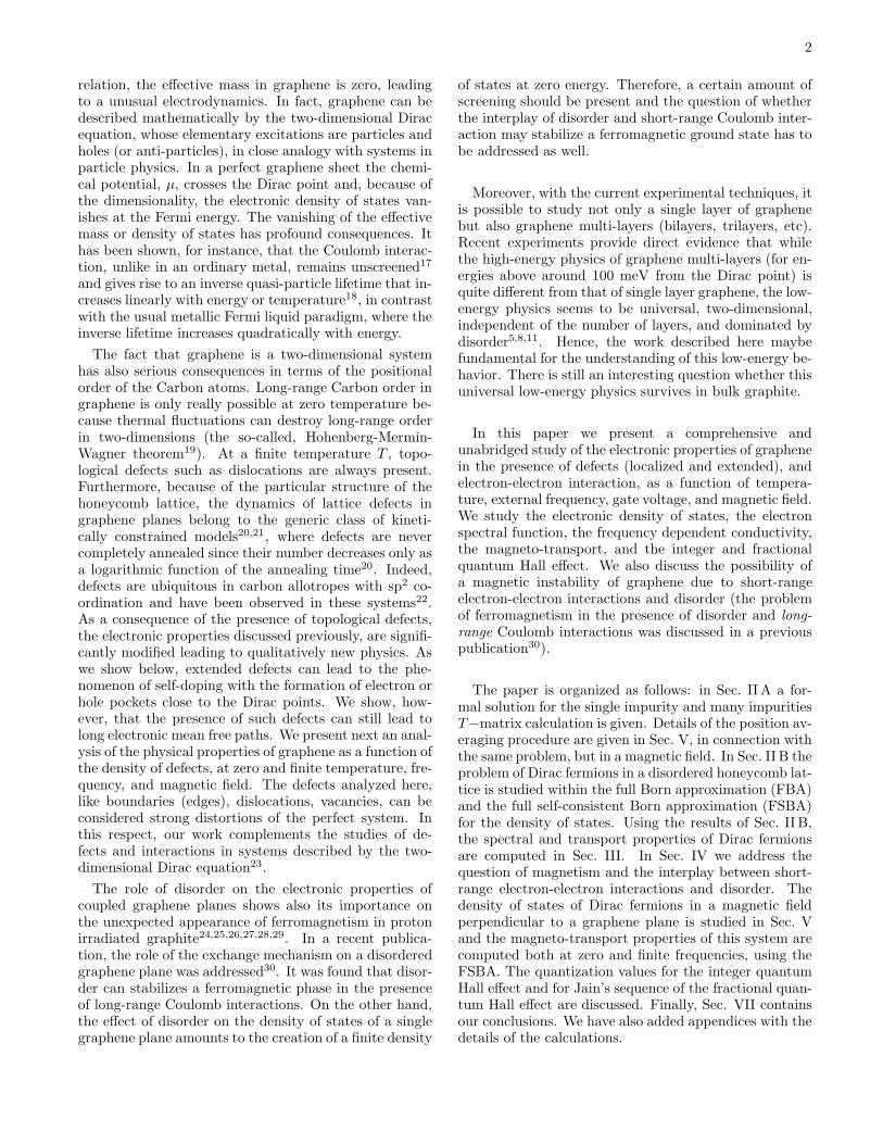
Notice that the self-energy, Σ(ω), in (2.38) depends onni in a non-trivial way, since both the self-consistent F (ω)and ρ(ω) also depend on ni. The self-energy is depictedin Fig. 4 for various values of the dilution density ni.

III. SPECTRAL AND TRANSPORTPROPERTIES

The electronic spectral function is defined as:

A(k, ω) = − 1

πImG(k, ω + i0+) , (3.1)

7

-0.8 -0.6 -0.4 -0.2 0 0.2 0.4 0.6 0.8 ε / D

0

2.5

5

7.5

10

-Im

Σ(ε

) / (D

ni )

n i = 0.1

n i = 0.01

n i = 0.001

-0.8 -0.6 -0.4 -0.2 0 0.2 0.4 0.6 0.8ε / D

-3

-2

-1

0

1

2

3

Re

Σ(ε)

/ (D

ni )

FIG. 4: (color on line) Imaginary (left panel) and real (rightpanel) part of the self-energy obtained from the FSBA. Notethat both quantities are divided by Dni.

and can be interpreted as the probability density thatan electron has momentum k and energy ω. For a non-interacting, non-disordered, problem, the spectral func-tion is simply a Dirac delta function at ω = E(k). Inthe presence of disorder and/or electron-electron interac-tions the spectral function is broadened and its sharpnessdetermines whether the electronic system supports quasi-particles. The spectral function can be measured directlyin angle resolved photoemission experiments (ARPES)38.

In terms of the self-energy, Σ(k, ω), the spectral func-tion reads:

A(k, ω) = − 1

π

ImΣ(k, ω)

[ω − E(k) − ReΣ(k, ω)]2 + [ImΣ(k, ω)]2.(3.2)

In the case of graphene, there are two contributions tothe self-energy,

Σ(k, ω) = Σe.−e.(k) + Σdis.(ω) , (3.3)

where Σe.−e.(k) is the self-energy correction due to theelectron-electron interactions that was computed origi-nally in Ref. [39]:

ImΣe.−e.(k) =1

48

(

e2

ǫ0vF

)2

vF |k| , (3.4)

where e is the electron charge, and ǫ0 the dielectric con-stant of graphene. The other contribution, Σdis., is dueto disorder and is given in (2.38).

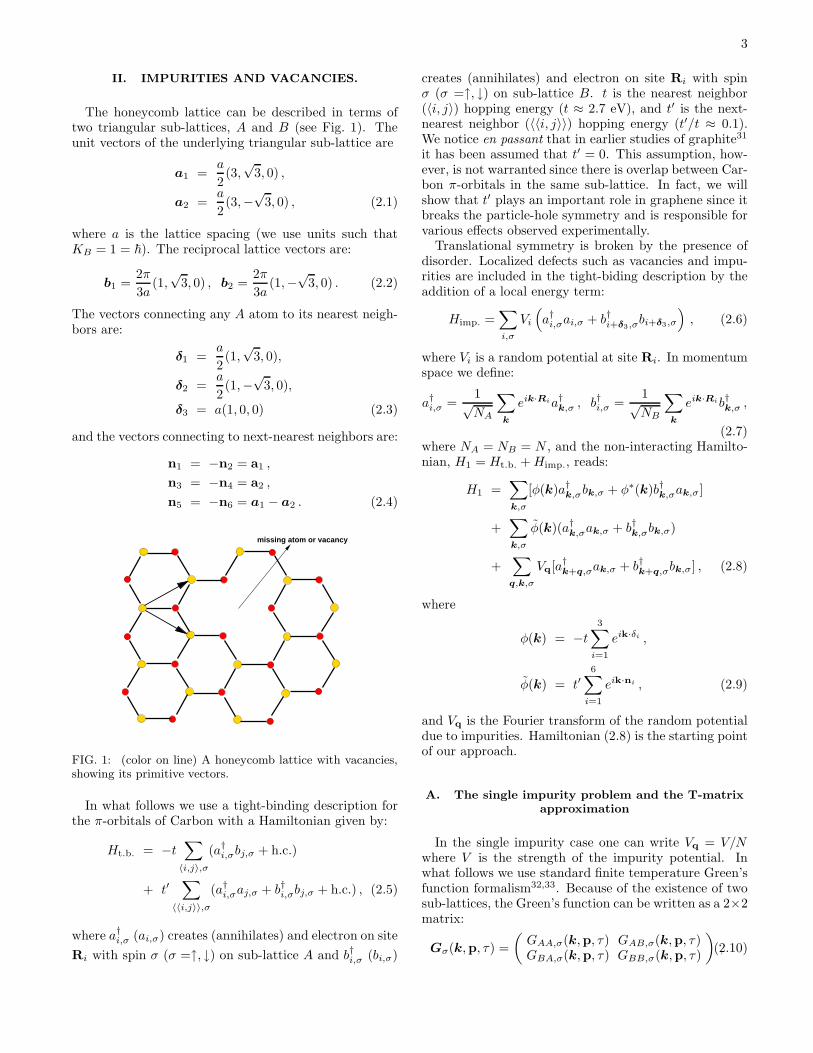
Notice that these two contributions to the self-energyhave very different dependence with the energy: while theelectron-electron self-energy decreases as the energy (mo-mentum) decreases, the self-energy due to disorder in-creases as the energy decreases. Hence, electron-electroninteractions are dominant at high energies while disorderis dominant at low energies. This interplay between thetwo self-energies leads to the prediction that there will bea minimum in the self-energy for some energy where the

FIG. 5: (color on line) Imaginary part of the electron’s selfenergy including both the effect of disordered and electron-electron interaction. The inset shows an intensity plot for thespectral function A(k, ω) for D = 8.248 eV , ni = 0.0001.

electron-electron interaction becomes of the same orderof the electron-vacancy interaction. In Fig. 5 we plot theself-energy as a function of energy for various impurityconcentrations together with the spectral function (in-set). One can clearly observe the non-monotonic depen-dence of the self-energy with the energy. This behaviorshould be observable in ARPES experiments.

Assuming an electric field applied in the x-direction,the frequency dependent (real part) conductivity is cal-culated from the Kubo formula:

σ(q, ω) =1

ω

∫ ∞

0

dteiωt〈[J†x(q, t), Jx(q, 0)]〉 (3.5)

where Jx is the x-component of the current operatorwhich, due to gauge invariance, has the form40:

Jx = −ite∑

i,σ,δ

ux · δa†i,σbi+δ,σ − ux · δb†i,σ+δai,σ (3.6)

(the notation i + δ means Ri + δ). In Fourier space,and after expanding the general expression around theK-point in the Brillouin zone, we obtain:

Jx = −ivF e∑

k,σ

(e−iπ/3a†k,σbk,σ − eiπ/3b†k,σak,σ) . (3.7)

Substitution of (3.7) into (3.5) shows that the problemdepends on the Green’s functions defined in (2.11). How-ever, due to the special form of Eq. (2.22) the conduc-tivity does not have contributions coming from productsof Green’s functions of the form GABGBA. Taking intoaccount the number of bands and the spin degeneracy,the Kubo formula for the real part of the conductivity atfinite frequency and temperature has the form:

σ(ω, T ) = − 4v2F e

2

NAcω

∫ ∞

−∞

dǫ

2π[f(ǫ+ ω) − f(ǫ)] ×

∑

k

ImGAA(k, ǫ+ i0+)ImGAA(k, ǫ+ ω + i0+) , (3.8)

8

-0.5 -0.25 0 0.25 0.5 ε / D

2

3

4

5

6K

(ε)

n i = 0.001

n i = 0.01

n i = 0.1

D=2 eV

-0.2 -0.1 0 0.1 0.20

10

20

30

40

50

60

-f ’(

ε) K

(ε)

T = 300 K

-0.005 -0.0025 0 0.0025 0.005ε / D

0

100

200

300

400

500

600

-f ’(

ε)K

(ε)

T= 10 K

FIG. 6: (color on line) Left: Kernel of the integral for σ(0, T )as function of the energy. Product of the Fermi functionderivative by K(ǫ) at two different temperatures.

where f(ǫ) = 1/(e(ǫ−µ)/T + 1) is the Fermi-Dirac dis-tribution function. The integral over k in (3.8) can beperformed and find:

σ(ω, T ) = − e2

2π2ω

∫ ∞

−∞

dǫ[f(ǫ+ ω) − f(ǫ)]K(ω, ǫ) ,(3.9)

where

K(ω, ǫ) = ImΣ(ǫ+ ω) ImΣ(ǫ) Θ(ω, ǫ) , (3.10)

(Θ(ω, ǫ) defined in Appendix A).It is instructive to consider the zero-temperature, zero-

frequency limit of the conductivity in Eq. (3.8) (restoring~):

σ0 =2

π

e2

h

(

1 − [ImΣ(0)]2

D2 + [ImΣ(0)]2

)

≈ 2

π

e2

h. (3.11)

The result (3.11) shows that as long as ImΣ(0) ≪D, σ0 has a universal value independent of the dilu-tion concentration, in agreement with earlier theoreticalworks41,42, and in agreement with the experimental datain graphene6.

At finite temperatures the integral in (3.9) has to beevaluated numerically. Consider σ(0, T ) whose behavioris determined by K(ǫ) ≡ K(0, ǫ). The quantities K(ǫ)and −f ′(ǫ)K(ǫ) ( −f ′(ǫ) is the derivative of the Fermifunction in order to ǫ) are both represented in Fig. 6. Thebehavior of K(ǫ) shows, “V”-like shape as the energy ǫis varied. As a consequence, σ(0, 0) should present thesame “V”-like shape as the chemical potential µ movesaround µ = 0. Such behavior has indeed been observedin atomically thin carbon films4,6, where the density ofelectrons was controled by a gate potential. The temper-ature dependence of the σ(0, T ), for µ = 0, is depictedin Fig. 7 for different vacancy concentrations, and it isfound to follow Sommerfeld asymptotic expansion, but

0 50 100 150 T (kelvin)

2

2.5

3

π σ

(T)

h / e

2

ni = 0.001

ni = 0.01

ni = 0.1

D = 2 eV

0 50 100 150 200 250 300 T (kelvin)

2

2.5

3

ni = 0.1

ni = 0.01

ni = 0.001

D = 1 eV

FIG. 7: (color on line) Dependence of σ(T, 0) on the temper-ature and on the impurity dilution ni.

the number of terms needed to fit the numerical curvegrows very fast as the dilution is reduced.

In Fig. 8 we plot the frequency dependence of σ(ω, T )obtained from numerical integration of (3.9) with the self-energy given in (2.38). At low temperature, we see thatσ(ω, T ) develops a maximum around an energy value thatis dependent on the number of impurities. In fact, ifplot σ(ω, T ) as function of ω/

√ni, the conductivity al-

most shows scaling behavior for all impurity dilutions(see lower left panel). As the temperature increases, andif σ(0, T ) is sufficiently large, the conductivity σ(ω, T )acquires a Drude-like behavior (right panel).

0 500 1000 1500

ω (cm-1

)

2

2.2

2.4

2.6

π σ

(ω,T)

h /

e2

ni = 0.0001

ni = 0.001

ni = 0.01

ni = 0.1

D = 1 eV, T = 10 K

10 100 1000

ω (cm-1

)

0

5

10

15

20

25

30

35

40

45

50

Drude fit

D = 1 eV, T = 100 K

0 5000 10000 15000

ω / (ni ) 1/2

(cm-1

)

2

2.2

2.4

2.6

FIG. 8: (color on line) Dependence of σ(T, ω) (in units ofe2/(π~)) , on the frequency ω.

9

IV. MAGNETIC RESPONSE AND THE ROLEOF SHORT RANGE COULOMB INTERACTIONS

The ferromagnetism measured in proton irradiatedgraphite opens the question whether the interplay of in-teractions and disorder can drive the system from a para-magnetic to a magnetic ground state15. We study theeffect of disorder on the magnetic susceptibility in thepresence of short-range interactions, and the resultingchange in the tendency towards magnetic instabilities.The problem of magnetic instabilities due to long-rangeexchange interactions43 in the presence of small densityof carriers was discussed in great detail in ref. [30]. Wedo not address here the effects associated to the interplaybetween the long-range Coulomb interaction and differ-ent types of lattice disorder44 and the appearance of localmoments close to defects45,46,47,48.

The paramagnetic susceptibility of graphene is givenby:

χ(T ) =∂mz

∂h= 4

∂

∂h

1

N

∑

k

∑

n

GAA(k, iωn − h)

= −4

∫ ∞

−∞

dǫf ′(ǫ)ρ(ǫ) , (4.1)

where

mz(T ) = 2∑

i,σ

σ〈a†i,σai,σ〉 , (4.2)

is the magnetization, and ρ(ǫ) is the electronic densityof states which, in the presence of disorder, is given in(2.40). Within the Stoner mechanism49, ferromagnetismis possible if the local electron-electron interaction term(the so-called Hubbard term)50, U , is large than a criticalvalue given by:

1

U cF

=1

4χ(0) . (4.3)

In the case of an antiferromagnetic instability the samecriteria would lead to another critical value of U givenby:

1

U cAF

=2

πD

∫ D

−∞

dǫρ(ǫ) arctan

[

D

ImΣ(ǫ)

]

. (4.4)

Notice that in the case of antiferromagnetism one findsthat U c

AF ≈ D/(1 − ni) when ImΣ → 0, in agreementwith Hartree-Fock calculations51.

In Fig. 9 we plot the magnetic susceptibility as functionof T for different values of ni. The signature of the pres-ence of Dirac fermions comes from the linear dependenceon T for T/D ≪ 1. Notice that, unlike the case of anordinary metal that has a temperature dependent Paulisusceptibility, the graphene susceptibility increases withtemperatures and number of impurities. At low temper-atures χ(T ) presents a small upturn not visible in Fig. 9.From the value of χ(0) and (4.3) we obtain the critical in-teraction required for a ferromagnetic transition, which

is shown in the lower left panel of Fig. 9. Notice thatthe critical interaction strength for ferromagnetism de-creases as the vacancy concentration increases indicatingthat disorder favors a ferromagnetic transition.

Using (4.4) and the results of the previous sections wecan also calculate the critical value for an antiferromag-netic transition. The result is shown in the lower rightpanel of Fig. 9. In contrast with the ferromagnetic case,the antiferromagnetic instability is suppressed by disor-der, requiring a large value of the electron-electron inter-action. Notice that the value of the critical ferromagneticcoupling is always bigger than the antiferromagnetic one,indicating that at half-filling the graphene lattice is moresusceptible to antiferromagnetic correlations. This resultis consistent with an old proposal by Linus Pauling thatgraphene should be a resonant valence bond (RVB) statewith local singlet correlations16.

0.1 0.2 0.3 0.4 0.5 0.6 0.7 0.8 0.9 T/D

0

0.2

0.4

0.6

0.8

1

1.2

1.4

Dχ(

T) ni = 0

ni = 0.1

ni = 0.01

ni = 0.001

0 0.02 0.04 0.06 0.08 0.1 ni

5

10

15

20

UF

0 0.05 0.1 0.15 0.2 ni

1

1.05

1.1

1.15

1.2

1.25

1.3

UA

F

FIG. 9: (color on line) Top: Dependence of χ(T ) on thetemperature and on the impurity dilution ni. Bottom: De-pendence of UF and UAF (in units of D) as function of ni.

Hence, the Stoner criteria seems to be unable to ex-plain the ferromagnetic behavior observed experimen-tally. One might ask whether additional scatteringmechanisms, such that provided by long-range electron-electron interactions, can modify the critical values of thecouplings. The self-energy correction due to long-rangeelectron-electron scattering is given in (3.4) and can beadded to the Dyson equation for the Green’s functionand a new self-consistent density of states can be com-puted. This approach does not modify the value of U c

F

which is determined by the low frequency behavior ofthe self-energy. In case of antiferromagnetism we findthat indeed it leads to an increase on U c

AF , but the re-sult is non-conservative since the integral over the den-sity of states gives a smaller value than (1 − ni). There-fore, we find from these calculations and previous ones30

that graphene is not particularly susceptible to ferromag-netism.

10

V. MAGNETO-TRANSPORT

The description of the magneto-transport properties ofelectrons in a disordered honeycomb lattice is complexbecause of the interference effects associated with theHofstadter problem52. As in the previous sections, wesimplify our problem by describing the electrons in thehoneycomb lattice as Dirac fermions in the continuum.A similar approach was considered by Abrikosov in thequantum magnetoresistance study of non-stoichiometricchalcogenides53. In the case of graphene, the effectiveHamiltonian describing Dirac fermions in a magnetic field(including disorder) can be written as: H = H0+Hi with

H0 = −vF

∑

i=x,y

σi[−i∂i + eAi(r)] , (5.1)

where, in the Landau gauge, (Ax, Ay, Az) = (−By, 0, 0)is the vector potential for a constant magnetic field B inthe z−direction, σi is the i = x, y, z Pauli matrix, and

Hi = V

Ni∑

j=1

δ(r − rj)I . (5.2)

The formulation of the problem in second quantizationrequires the solution of H0, which is sketched in Ap-pendix B. The field operators are defined as (see Ap-pendix B for notation; the spin index is omitted for sim-plicity):

Ψ(r) =∑

k

eikx

√L

(

0φ0(y)

)

ck,−1

+∑

n,k,α

eikx

√2L

(

φn(y − kl2B)φn+1(y − kl2B)

)

ck,n,α . (5.3)

The sum over n = 0, 1, 2, . . . , is cut off at an n0 givenby E(1, n0) = D. In this representation H0 becomesdiagonal, leading to Green’s functions of the form (inMatsubara representation):

G0(k, n, α; iω) =1

iω − E(α, n), (5.4)

is effectively k-independent, and E(α,−1) = 0 is the zeroenergy Landau level. The part of Hamiltonian due to theimpurities is written as:

Hi =V

L

Ni∑

j=1

∑

p,k

e−ixj(p−k)

[

φ0(yj − pl2B)φ0(yj − kl2B)c†p,−1ck,−1 +∑

n,α

α√2φ0(yj − pl2B)φn+1(yj − kl2B)c†p,−1ck,n,α

+∑

n,α

α√2φn+1(yj − pl2B)φ0(yj − kl2B)c†p,n,αck,−1

+∑

n,m,α,λ

1

2[φn(yj − pl2B)φm(yj − kl2B) + αλφn+1(yj − pl2B)φm+1(yj − kl2B)]c†p,n,αck,m,λ

. (5.5)

Equation (5.5) describes the elastic scattering of electronsin Landau levels by the impurities. It is worth noting thatthis type of scattering connects Landau levels of negativeand positive energy.

A. The full self-consistent Born approximation

In order to describe the effect of impurity scatter-ing on the magnetoresistance of graphene, the Green’sfunction for Landau levels in the presence of disorderneeds to be computed. In the context of the 2D elec-tron gas, an equivalent study was performed by Othaand Ando,54,55,56using the averaging procedure over im-purity positions of Duke57. Here the averaging proce-dure over impurity positions is performed in the standardway, namely, having determined the Green’s function fora given impurity configuration (r1, . . .rNi

), the positionaveraged Green’s function is determined from (as in Sec.

II A):

〈G(p, n, α; iω; r1, . . .rNi)〉 ≡ G(p, n, α; iω)

= L−2Ni

Ni∏

j=1

∫

drj

G(p, n, α; iω; r1, . . .rNi) . (5.6)

In Sec. II A the averaging involved plane wave states;in the presence of Landau levels the average over im-purity positions involves the wave functions of the one-dimensional harmonic oscillator. In the averaging proce-dure we have used the following identities:

∫

dyφn(y − pl2B)φm(y − pl2B) = δn,m , (5.7)

∫

dpφn(y − pl2B)φm(y − pl2B) =δn,m

l2B. (5.8)

11

0

0.002

0.004

0.006

0.008 D

OS

per

u.c

. (1/

eV)

ni = 0.001

ni = 0.005

ni = 0.0009

ωc = 0.14 eV, T = 12 T

-3 -2 -1 0 1 2 3ω / ωc

0

0.002

0.004

0.006

0.008

DO

S p

er u

.c. (

1/eV

)

ni = 0.001

ni = 0.0008

ni = 0.0006

ωc = 0.1 eV, B = 6 T

FIG. 10: (color on line) Electronic density of states in amagnetic field for different dilutions and magnetic field. Thenon-disordered DOS and the position of the Landau levelsin the absence of disorder are also shown. The two arrows inthe upper panel show the position of the renormalized Landaulevels (see Fig.11) given by the solution of Eq. (5.14). Theenergy is given in units of ωc ≡ E(1, 1).

After a lengthy algebra, the Green’s function in the pres-ence of vacancies, in the FSBA, can be written as:

G(p, n, α;ω + 0+) = [ω − E(n, α) − Σ1(ω)]−1 ,(5.9)

G(p,−1;ω + 0+) = [ω − Σ2(ω)]−1 , (5.10)

where

Σ1(ω) = −ni[Z(ω)]−1 , (5.11)

Σ2(ω) = −ni[gcG(p,−1;ω + 0+)/2 + Z(ω)]−1 ,(5.12)

Z(ω) = gcG(p,−1;ω + 0+)/2

+ gc

∑

n,α

G(p, n, α;ω + 0+)/2 , (5.13)

and gc = Ac/(2πl2B) is the degeneracy of a Landau level

per unit cell. One should notice that the Green’s func-tions do not depend upon p explicitly. The self-consistentsolution of Eqs. (5.9), (5.10), (5.11), (5.12) and (5.13)gives density of states, the electron self-energy, and therenormalization of Landau level energy position due todisorder.

The effect of dilution in the density of states of Diracfermions in a magnetic field is shown in Fig. 10. Forreference we note that E(1, 1) = 0.14 eV, for B = 14T, and E(1, 1) = 0.1 eV, for B = 6 T. From Fig. 10we see that given an impurity concentration the effectof broadening due to vacancies is less effective as themagnetic field increases. It is also clear that the positionof Landau levels is renormalized relatively to the non-disordered case. The renormalization of the Landau levelposition can be determined from poles of (5.10):

ω − E(α, n) − ReΣ(ω) = 0 . (5.14)

Of course, due to the importance of scattering at lowenergies, the solution to Eq. (5.14) does not representexact eigenstates of system since the imaginary part ofthe self-energy is non-vanishing, however these energiesdo determine the form of the density of states, as wediscuss below.

In Fig. 11, the graphical solution to Eq. (5.14) is givenfor two different energies (E(−1, n), with n = 1, 2), beingclear that the renormalization is important for the firstLandau level. This result is due to the increase of thescattering at low energies, which is present already in thecase of zero magnetic field. The values of ω satisfying Eq.(5.14) show up in density of states as the energy valueswhere the oscillations due to the Landau level quantiza-tion have a maximum. In Fig. 10, the position of therenormalized Landau levels is shown in the upper panel(marked by two arrows), corresponding to the bare en-ergies E(−1, n), with n = 1, 2. The importance of thisrenormalization decreases with the reduction of numberof vacancies. This is clear in Fig. 10 where a visible shifttoward low energies is evident when ni has a small 10%change, from ni = 10−3 to ni = 9 × 10−4.

-6 -4 -2 0 2 4 60

0.2

0.4

0.6

0.8

-Im

Σ1(ω

) / ω

c B = 12 T B = 6 T

ni=0.001

-6 -4 -2 0 2 4 6

-0.4

-0.2

0

0.2

0.4

Re

Σ 1(ω) /

ωc

ω−E(-1,1)ω−E(-1,2)

-6 -4 -2 0 2 4 6ω / ωc

0

0.2

0.4

0.6

0.8

-Im

Σ2(ω

) / ω

c

-6 -4 -2 0 2 4 6ω / ωc

-0.4

-0.2

0

0.2

0.4

Re

Σ 2(ω) /

ωc ω

FIG. 11: (color on line) Self-consistent results for Σ1(ω) (top)and Σ2(ω)(bottom). The energy is given in units of ωc ≡E(1, 1). In the left panels we show the intercept of ω−E(α, n)with ReΣ(ω) as required in (5.14).

B. Calculation of the transport properties

The study of the magnetoresistance properties of thesystem requires the calculation of the conductivity ten-sor. In terms of the field operators, the current densityoperator j is given by18:

j = vF e[Ψ†(x, y)σxΨ(x, y),Ψ†(x, y)σyΨ(x, y)] , (5.15)

leading to current operator in the Landau basis writtenas:

12

Jx = vF e∑

p,α

1√2

[

c†p,−1ck,0,α + c†p,0,αcp,−1

]

+ vF e∑

p,n,α,λ

1

2

[

λ(1 − δn,0)c†p,n,αcp,n−1,λ + αc†p,n,αcp,n+1,λ

]

, (5.16)

Jy = vF e∑

p,α

i√2

[

c†p,−1ck,0,α − c†p,0,αcp,−1

]

+ vF e∑

p,n,α,λ

i

2

[

−λ(1 − δn,0)c†p,n,αcp,n−1,λ + αc†p,n,αcp,n+1,λ

]

.(5.17)

As in Sec. III, we compute the current-current correlation function and from it the conductivity tensor is derived.The diagonal component of the conductivity tensor σxx(ω, T ) is given by (with the spin included):

σxx(ω, T ) = −4(vF e)2

2πl2B

1

ω

∫ ∞

−∞

dǫ

2π[f(ǫ+ ω) − f(ǫ)]

[

1

2

∑

α1

[ImG(−1; ǫ+ i0+)ImG(0, α; ǫ+ ω + i0+)

+ ImG(0, α; ǫ+ i0+)ImG(−1; ǫ+ ω + i0+)] +1

4

∑

n≥1,α,λ

ImG(n, α; ǫ+ i0+)ImG(n− 1, λ; ǫ+ ω + i0+)

+1

4

∑

n≥0,α,λ

ImG(n, α; ǫ+ i0+)ImG(n+ 1, λ; ǫ+ ω + i0+)

, (5.18)

and the off-diagonal component σxy(ω, T ) of the conductivity tensor is given by:

σxy(ω, T ) =2(vF e)

2

4πl2B

1

ω

∫ ∞

−∞

dǫ

2πtanh

( ǫ

2T

)

∑

α,γ

[

γ[ReG(0, α; ǫ+ γω + i0+)ImG(−1; ǫ+ i0+)

− ReG(−1; ǫ+ γω + i0+)ImG(0, α; ǫ+ i0+)] +∑

λ,n≥1

γ

2[ReG(n, α; ǫ+ γω + i0+)ImG(n− 1, λ; ǫ+ i0+)

− ReG(n− 1, α; ǫ+ γω + i0+)ImG(n, λ; ǫ+ i0+)]]

. (5.19)

If we neglect the real part of the self-energy, and assumeImΣi(ω) = Γ = constant (i = 1, 2), and let ω → 0, Eq.(5.18) reduces to Eq. (85) in Ref. [58], if we furtherassume the case E(1, 1) ≫ Γ then Eq. (5.19) reduces toEq. (86) of the same reference.

As in Sec. III, it is instructive to consider first the caseω, T → 0, which leads to (σxx(0, 0) = σ0):

σ0 =e2

h

2

π

[

ImΣ1(0)/ImΣ2(0) − 1

1 + (ImΣ1(0)/ωc)2

+n0 + 1

n0 + 1 + (ImΣ1(0)/ωc)2

]

. (5.20)

When ImΣ1(0) ≃ ImΣ2(0) and ωc ≫ ImΣ1(0) (or n0 ≫ImΣ1(0)/ωc), with ωc = E(0, 1) =

√2vF /l

2B, Eq. (5.20)

reduces to: σ0 ≃ 2/π(e2/h), which is identical to theresult (3.11) in the absence of the field found in Sec.III. This result was obtained previously by Ando andcollaborators using the second order self-consistent Bornapproximation59,60. However, in the FSBA it is requiredthat the above conditions be satisfied for this result tohold. From Fig. 12 we see that the above conditions holdapproximately over a wide ranges of field strength.

Because the d.c. magneto-transport properties havebeen measured graphene samples4 subjected to a gatepotential (allowing to tune the electronic density), it isimportant to compute the conductivity kernel, since this

has direct experimental relevance. In the the case ω → 0we write the conductivity σxx(0, T ) as:

σxx(0, T ) =e2

πh

∫ ∞

−∞

dǫ∂f(ǫ)

∂ǫKB(ǫ) , (5.21)

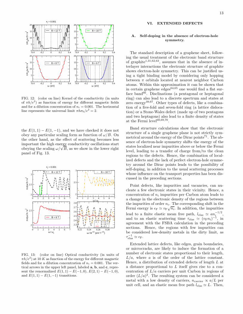
where the conductivity kernelKB(ǫ) is given is AppendixA. The magnetic field dependence of kernel KB(ǫ) isshown in Fig. 12. Observe that the effect of disorder isthe creation of a region where KB(ǫ) remains constantbefore it starts to increase in energy with superimposedoscillations coming from the Landau levels. The sameeffect, but with the absence of the oscillations, was iden-tified at the level of the self-consistent density of statesplotted in Fig. 10. Together with σxx(0, T ), the Hallconductivity σxy(0, T ) allows the calculation of the resis-tivity tensor:

ρxx =σxx

σ2xx + σ2

xy

,

ρxy =σxy

σ2xx + σ2

xy

. (5.22)

Let us now focus on the optical conductivity, σxx(ω).This quantity can be probed by reflectivity experimentson the sub-THz to Mid-IR frequency range.61 We depictthe behavior of Eq. (5.18) in Fig. 13 for different mag-netic fields. It is clear that the first peak is controlled by

13

-0.4 -0.2 0 0.2 0.40

5

10

15

20π

KB(ω

) h /

e2 B = 12 T

ni = 0.001

-0.4 -0.2 0 0.2 0.40

5

10

15

20

B = 10 T

-0.4 -0.2 0 0.2 0.4ω (eV)

0

5

10

15

20

π K

B(ω

) h /

e2 B = 8 T

-0.4 -0.2 0 0.2 0.4ω (eV)

0

5

10

15

20

B = 6 T

FIG. 12: (color on line) Kernel of the conductivity (in unitsof πh/e2) as function of energy for different magnetic fieldsand for a dilution concentration of ni = 0.001. The horizontalline represents the universal limit πhσ0/e2 = 2.

the E(1, 1) − E(1,−1), and we have checked it does notobey any particular scaling form as function of ω/B. Onthe other hand, as the effect of scattering becomes lessimportant the high energy conductivity oscillations startobeying the scaling ω/

√B, as we show in the lower right

panel of Fig. 13.

0 1 2 3 4 5 6 7

2

2.5

3

π σ

(ω) h

/ e2

B = 12 T

ni = 0.001

0 1 2 3 4 5 6 7ω / ωc

2

2.5

3 B = 10 T

0 1 2 3 4 5 6 7ω / ωc

2

2.5

π σ

(ω) h

/ e2

B = 6 T

0.22 0.24 0.26 0.28

ω / B 1/2 (eV/ T

1/2)

2.3

2.4

2.5

2.6

2.7

2.8

B = 12 T B = 10 T B = 6 T

ab

c

FIG. 13: (color on line) Optical conductivity (in units ofπh/e2) at 10 K as function of the energy for different magneticfields and for a dilution concentration of ni = 0.001. The ver-tical arrows in the upper left panel, labeled a, b, and c, repre-sent the renormalized E(1, 1) −E(−1, 0), E(2, 1)− E(−1, 0),and E(1, 1) − E(1,−1) transitions.

VI. EXTENDED DEFECTS

A. Self-doping in the absence of electron-holesymmetry.

The standard description of a graphene sheet, follow-ing the usual treatment of the electronic band structureof graphite1,31,62,63, assumes that in the absence of in-terlayer interactions the electronic structure of graphiteshows electron-hole symmetry. This can be justified us-ing a tight binding model by considering only hoppingbetween π orbitals located at nearest neighbor Carbonatoms. Within this approximation it can be shown thatin certain graphene edges64,65 one would find a flat sur-face band66. Disclinations (a pentagonal or heptagonalring) can also lead to a discrete spectrum and states atzero energy39,67. Other types of defects, like a combina-tion of a five-fold and seven-fold ring (a lattice disloca-tion) or a Stone-Wales defect (made up of two pentagonsand two heptagons) also lead to a finite density of statesat the Fermi level68,69,70.

Band structure calculations show that the electronicstructure of a single graphene plane is not strictly sym-metrical around the energy of the Dirac points71. The ab-sence of electron-hole symmetry shifts the energy of thestates localized near impurities above or below the Fermilevel, leading to a transfer of charge from/to the cleanregions to the defects. Hence, the combination of local-ized defects and the lack of perfect electron-hole symme-try around the Dirac points leads to the possibility ofself-doping, in addition to the usual scattering processeswhose influence on the transport properties has been dis-cussed in the preceding sections.

Point defects, like impurities and vacancies, can nu-cleate a few electronic states in their vicinity. Hence, aconcentration of ni impurities per Carbon atom leads toa change in the electronic density of the regions betweenthe impurities of order ni. The corresponding shift in theFermi energy is ǫF ≃ vF

√ni. In addition, the impurities

lead to a finite elastic mean free path, lelas ≃ an−1/2i ,

and to an elastic scattering time τelas ≃ (vFni)−1, in

agreement with the FSBA calculation in the precedingsections. Hence, the regions with few impurities canbe considered low-density metals in the dirty limit, asτ−1elas ≃ ǫF.

Extended lattice defects, like edges, grain boundaries,or microcracks, are likely to induce the formation of anumber of electronic states proportional to their length,L/a, where a is of the order of the lattice constant.Hence, a distribution of extended defects of length L ata distance proportional to L itself gives rise to a con-centration of L/a carriers per unit Carbon in regions oforder (L/a)2. The resulting system can be considered ametal with a low density of carriers, ncarrier ∝ a/L perunit cell, and an elastic mean free path lelas ≃ L. Then,

14

we obtain:

ǫF ≃ vF√aL

1

τelas≃ vF

L(6.1)

and, therefore, (τelas)−1 ≪ ǫF when a/L ≪ 1. Hence,

the existence of extended defects leads to the possibil-ity of self-doping but maintaining most of the samplein the clean limit. In this regime, coherent oscillationsof the transport properties are to be expected, althoughthe observed electronic properties will correspond to ashifted Fermi energy with respect to the nominally neu-tral defect–free system.

B. Electronic structure near extended defects.

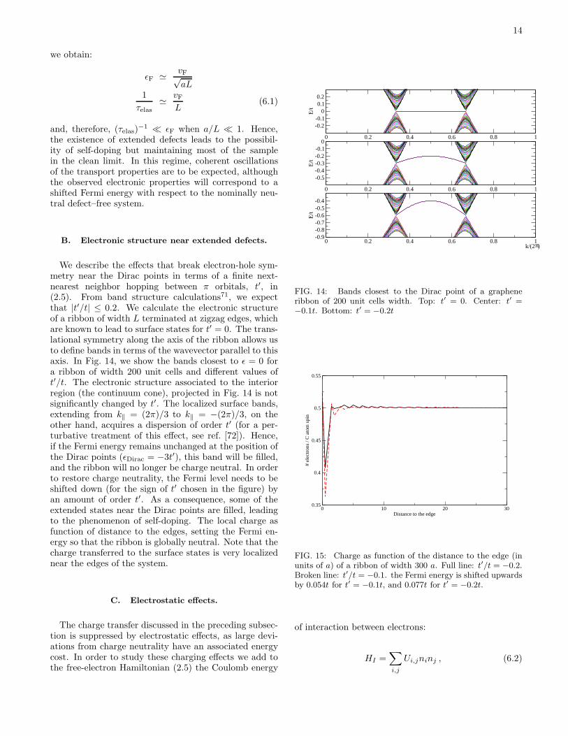
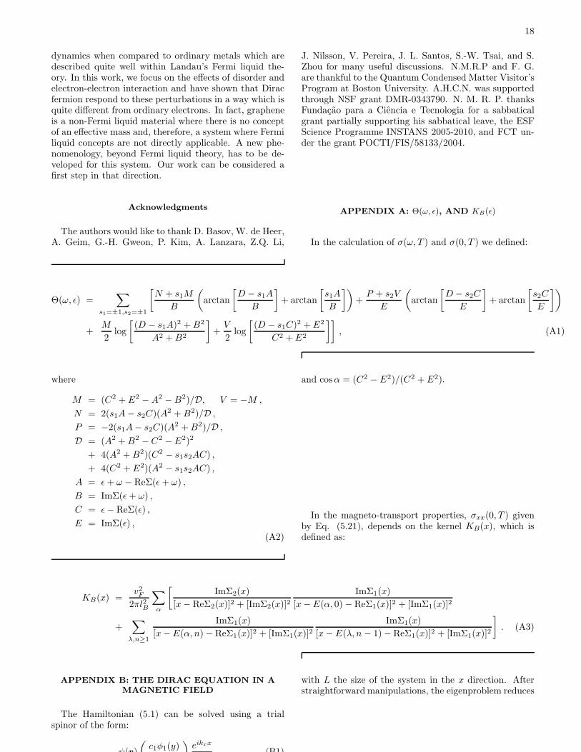
We describe the effects that break electron-hole sym-metry near the Dirac points in terms of a finite next-nearest neighbor hopping between π orbitals, t′, in(2.5). From band structure calculations71, we expectthat |t′/t| ≤ 0.2. We calculate the electronic structureof a ribbon of width L terminated at zigzag edges, whichare known to lead to surface states for t′ = 0. The trans-lational symmetry along the axis of the ribbon allows usto define bands in terms of the wavevector parallel to thisaxis. In Fig. 14, we show the bands closest to ǫ = 0 fora ribbon of width 200 unit cells and different values oft′/t. The electronic structure associated to the interiorregion (the continuum cone), projected in Fig. 14 is notsignificantly changed by t′. The localized surface bands,extending from k‖ = (2π)/3 to k‖ = −(2π)/3, on theother hand, acquires a dispersion of order t′ (for a per-turbative treatment of this effect, see ref. [72]). Hence,if the Fermi energy remains unchanged at the position ofthe Dirac points (ǫDirac = −3t′), this band will be filled,and the ribbon will no longer be charge neutral. In orderto restore charge neutrality, the Fermi level needs to beshifted down (for the sign of t′ chosen in the figure) byan amount of order t′. As a consequence, some of theextended states near the Dirac points are filled, leadingto the phenomenon of self-doping. The local charge asfunction of distance to the edges, setting the Fermi en-ergy so that the ribbon is globally neutral. Note that thecharge transferred to the surface states is very localizednear the edges of the system.

C. Electrostatic effects.

The charge transfer discussed in the preceding subsec-tion is suppressed by electrostatic effects, as large devi-ations from charge neutrality have an associated energycost. In order to study these charging effects we add tothe free-electron Hamiltonian (2.5) the Coulomb energy

0 0.2 0.4 0.6 0.8 1

-0.2-0.1

00.10.2

E/t

0 0.2 0.4 0.6 0.8 1

-0.5-0.4-0.3-0.2-0.1

0

E/t

0 0.2 0.4 0.6 0.8 1-0.9-0.8-0.7-0.6-0.5-0.4

E/t

k/(2 )π

FIG. 14: Bands closest to the Dirac point of a grapheneribbon of 200 unit cells width. Top: t′ = 0. Center: t′ =−0.1t. Bottom: t′ = −0.2t

0 10 20 30Distance to the edge

0.35

0.4

0.45

0.5

0.55

# el

ectr

ons

/ C a

tom

spi

n

FIG. 15: Charge as function of the distance to the edge (inunits of a) of a ribbon of width 300 a. Full line: t′/t = −0.2.Broken line: t′/t = −0.1. the Fermi energy is shifted upwardsby 0.054t for t′ = −0.1t, and 0.077t for t′ = −0.2t.

of interaction between electrons:

HI =∑

i,j

Ui,jninj , (6.2)

15

0 100 200 300 400 500Position

-0.04

-0.02

0

0.02

0.04

0.06

Ele

ctro

stat

ic p

oten

tial

0 10 200.4

0.45

0.5

0.5

0.5005

Cha

rge

dens

ity

0 200 400 600 800 1000 1200 1400Width

0

0.0001

0.0002

0.0003

0.0004

0.0005

Dop

ing

FIG. 16: Top: Self-consistent charge density (continuousline) and electrostatic potential (dashed line) of a grapheneribbon with periodic boundary conditions along the zig-zagedge and with a circumference of size W = 80

√3a, and a

length of L = 960a. The parameters used are described inthe text. The inset shows the details of the electronic densitynear the edge. Due to the presence of the edge, there is adisplaced charge in the bulk (bottom panel) that is shown asa function of the width W .

where ni =∑

σ(a†i,σai,σ+b†i,σbi,σ) is the number operatorat site Ri, and

Ui,j =e2

ǫ0|Ri − Rj |, (6.3)

is the Coulomb interaction between electrons. We expect,on physical grounds, that an electrostatic potential buildsup at the edges, shifting the position of the surface states,and reducing the charge transferred to/from them. Thepotential at the edge induced by a constant doping δper Carbon atom is roughly, ∼ (δe2/a)(W/a) (δe2/a isthe Coulomb energy per Carbon), and W the width ofthe ribbon (W/a is the number of Carbons involved).The charge transfer is arrested when the potential shiftsthe localized states to the Fermi energy, that is, whent′ ≈ (e2/a)(W/a)δ. The resulting self-doping is thereforeδ ∼ (t′a2)/(e2W ).

We treat the Hamiltonian (6.2) within the Hartree ap-proximation (that is, we replace HI by HM.F. =

∑

i Vini

where Vi =∑

j Ui,j〈nj〉, and solve the problem self-

consistently for 〈ni〉). Numerical results for graphene

ribbons of length L = 80√

3a and different widths areshown in Fig. 15 and Fig. 16 (t′/t = 0.2 and e2/a = 0.5t).The largest width studied is ∼ 0.1µm, and the total num-ber of carbon atoms in the ribbon is ≈ 105. Notice thatas W increases, the self-doping decreases indicating that,for a perfect graphene plane (W → ∞), the self-dopingeffect disappears. For realistic parameters, we find thatthe amount of self-doping is 10−4 − 10−5 electrons per

unit cell for domains of sizes 0.1 − 1µm, in agreementwith the amount of charge observed in these systems.

-0.9

-0.8

-0.7

-0.6

-0.5

-0.4

Ene

rgy

-0.9

-0.8

-0.7

-0.6

-0.5

-0.4

Ene

rgy

Momentum

-0.9

-0.8

-0.7

-0.6

-0.5

-0.4

Ene

rgy

π 2π0

FIG. 17: Electronic levels of a graphene ribbon with zig-zag edges in the presence of a magnetic field (t′ = −0.2t).The magnetic flux per hexagon of the honeycomb lattice isΦ = 0 (top), Φ = 0.00025 (center), and Φ = 0.0005 (bottom),in units of the quantum of magnetic flux, Φ0 = h/e. Thecorresponding magnetic fields are 0T, 60T and 120T.

D. Edge and surface states in the presence of amagnetic field.

We can analyze the electronic structure of a grapheneribbon of finite width in the presence of a magnetic field.The resulting tight binding equations can be consideredas an extension of the Hofstadter problem73 to a honey-comb lattice with edges. The bulk electronic structureis characterized by the Landau level structure discussedin previous sections. These states are modified at theedges, leading to chiral edge states, as discussed in rela-tion to the Integer Hall Effect (IQHE)74. The existenceof two Dirac points leads to two independent edge states,with the same chirality. In addition, Landau levels withpositive energy should behave in an electron-like fashion,moving upwards in energy as their “center of gravity” ap-proaches the edges. Landau levels with negative energyshould be shifted towards lower energy near the edges.

A zig-zag edge induces also a non-chiral surface band.If the width of these states is much smaller than themagnetic field they will not be much affected by the pres-ence of the field. The extension of the surface states iscomparable to the lattice spacing for most of the range|k‖| ≤ (2π)/3, except near the Dirac points, so that theeffect of realistic magnetic fields on these states is negli-gible.

The finite value of the second nearest neighbor hoppingt′ modifies the Landau levels obtained from the analysis

16

of the Dirac equation. Elementary calculations (as thosegiven in Appendix B) lead to:

E±(n) = −3t′ + 2l−2B α

(

n+1

2

)

±√

l−4B α2 + 2l−2

B γ2n ,

(6.4)with n = 0, 1, 2, 3, . . ., α = 9t′a2/4 and γ = 3ta/2, withthe single assumption that t ≫ t′. This solution pointsout a number of interesting aspects, the most importantof which is disappearance of the zero energy Landau level,made partially of holes and partially of electrons. Witht′, the electron or hole nature of the energy level becomesunambiguous, and half of the original zero energy Lan-dau level (with t′ = 0)moves down in energy (relativelyto the Fermi energy) and the other half moves up. Inaddition, the level spacing for electron and hole levelsbecomes unequal.

0 50 100 150 2000

0.020.040.060.08

0.1

0 50 100 150 2000

0.020.040.060.08

0.1

0 50 100 150 2000

0.020.040.060.08

0.1

0 50 100 150 2000

0.020.040.060.08

0.1

0 50 100 150 2000

0.020.040.060.08

0.1

0 50 100 150 2000

0.020.040.060.08

0.1

0 50 100 150 2000

0.020.040.060.08

0.1

0 50 100 150 2000

0.020.040.060.08

0.1

0 50 100 150 2000

0.020.040.060.08

0.1

0 50 100 150 2000

0.020.040.060.08

0.1

k=0 k=0.2 π

k=0.4 ππ

π

π

π

π

ππ

k=0.6

k=0.8 k=

k=1.2 k=1.4

k=1.6 k=1.8

FIG. 18: (Color online) Wave function of the lowest Landaulevels for different momenta. Black: n=0. Red: n=1. Green:n=2. Blue: n=3.

The presence of a magnetic field acting on the ribbondoes not break the translational symmetry along the di-rection parallel to the ribbon, that allows us to discussthe electronic structure in terms of the same bands cal-culated in the absence of the magnetic field. Resultsfor the ribbon analyzed in Fig. 14 for different magneticfields are shown in Fig. 17. The “center of gravity” ofthe wavefunctions associated to the levels moves in thedirection transverse to the ribbon as the momentum isincreased. The results show the bulk Landau levels, andtheir changes as the wavefunctions approach the edges.The surface band is practically unchanged, except forsmall avoided crossings every time that it becomes de-generate with a bulk Landau level. The results showquite accurately the expected scaling ǫn ∝ ±√

n for theeigenenergies derived from the Dirac equation, with smallcorrections due to lattice effects and a finite t′ (see Ap-pendix B). The corresponding wavefunctions for differentbands and momenta are shown in Fig. 18. The Landau

levels move rigidly towards the edges, where one also findsurface states.

We can compute the Hall conductivity from the num-ber of chiral states induced by the field at the edges74. Ifwe fix the chemical potential above the n-th level, thereare 2× (2n+ 1) edge modes crossing the Fermi level (in-cluding the spin degeneracy). Hence, the Hall conductiv-ity is:

σxy =e2

h2 × (2n+ 1) =

4e2

h(n+ 1/2) . (6.5)

This result should be compared with the usual IQHE inheterostructures, in which the factor of 1/2 is absent.The presence of this 1/2 factor is a direct consequenceof the presence of the zero mode in the Dirac fermionproblem. The existence of this anomalous IQHE was pre-dicted long ago in the context of high energy physics75,76

and more recently in the context of graphene12,14, butwas observed in graphene only recently by two indepen-dent groups6,11. An incomplete IQHE, with a finite lon-gitudinal resistivity, was observed in HOPG graphite77.

E. Fractional quantum Hall effect

While the IQHE depends only of the cyclotron energy,ωc, and therefore is a robust effect, the fractional quan-tum Hall effect (FQHE) is a more delicate problem sinceit is a result of electron-electron interactions. The prob-lem of electron-electron interactions in the presence of alarge magnetic field in a honeycomb lattice is a complexproblem that deserves a separate study. In this paper wemake a few conjectures about the structure of the FQHEbased on generic properties of Laughlin’s wave functions.

The electrons occupying the lowest Landau level areassumed to be in a many-body wavefunction written as(Ri = (xi, yi) and z = x+ iy)78 :

Ψ = exp(−i2m∑

i<j

αi,j)Φ(z1, . . . , zN ) , (6.6)

where αi,j = arctan[Im(zi − zj)/Re(zi − zj)],Φ(z1, . . . , zN ) is an anti-symmetric function of the inter-change of two z′s, and m = 0, 1, 2, . . .. The effect of thesingular phase associated with the many-body wave func-tion is to introduce an effective magnetic field B∗ givenby:

B∗ = B − ∇a(r)/e = B − 2π(2m)ρ(r)/e , (6.7)

where the gauge field a(r) is given by

a(ri) = 2m∑

j 6=i

∇(ri)αi,j , (6.8)

and ρ(r) is the electronic density. The procedure outlinedabove is called flux-attachment and leads to appearanceof composite fermions. These composite particles do not

17

feel the external field B but instead an effective field B∗.Therefore, the FQHE of electrons can be seen as an IQHEof these composite particles.

Given an electronic density δ, we may define an effec-tive filling factor p∗ for the composite particles as:

p∗ =2πδ

eB∗. (6.9)

In the lowest Landau level the electron filling factor is:

p =2πδ

eB, (6.10)

and combining Eqs. (6.9) and (6.10) we obtain:

p =p∗

2mp∗ + 1, (6.11)

so, we can write:

B∗ = B(1 − 2mp) . (6.12)

The crucial assumption in the case of graphene is thatthe effective p∗ associated with the integer quantum Halleffect of composite particles has the form given in (6.5),that is (spin ignored):

p∗ = (2n+ 1) , n = 0, 1, 2, 3, . . . , (6.13)

(the effective field B∗ is such that the system has oneor more filled composite particle Landau levels, and thechemical potential lies between two these) leading to aquantized Hall conductivity given by:

σxy =2n+ 1

2m(2n+ 1) + 1

2e2

h. (6.14)

For n = 0, one obtains the so-called Laughlin sequence:σxy = 1/(2m + 1)(2e2/h), and for m = 0 we recover(6.5). This argument shows that Jain’s sequence is quitedifferent from that of the 2D electrons gas79.

As in the case of the IQHE, the FQHE can be thoughtin terms of chiral edge states, or chiral Luttinger liquids,that circulate at the edge of the sample80. One can seethe IQHE and FQHE as direct consequences of the pres-ence of these edge states. Because of their chiral nature,edge states do not localize in the presence of disorderand hence the quantization of the Hall conductivity isrobust. In graphene, as we have discussed previously,zig-zag edges support surface states that are non-chiralLuttinger liquids. We have recently shown that electron-electron interactions between chiral Luttinger liquids andnon-chiral surface states can lead to instabilities of thechiral edge modes leading to edge reconstruction13 andhence to the destruction of the quantization of conduc-tivity. We also have shown that this edge reconstruc-tion depends strongly on the amount of disorder at theedge of the sample. While this effect is not strong in theIQHE (because the cyclotron energy is very large whencompared with the other energy scales), it makes the ex-perimental observation of the FQHE in graphene verydifficult.

VII. CONCLUDING REMARKS

To summarize, we have analyzed the influence of localand extended lattice defects in the electronic propertiesof single graphene layer. Our results show that: (1) Pointdefects, such as vacancies, lead to an enhancement of thedensity of states at low energies and to a finite densityof states at the Dirac point (in contrast to the clean casewhere the density of states vanishes); (2) Vacancies havea strong effect in the Dirac fermion self-energy leadingto a very short quasi-particle lifetime at low energies; (3)The interplay between local defects and electron-electroninteraction lead to the existence of a minimum in theimaginary part of the electron self-energy (a result thatcan be measured in ARPES); (4) The low temperatured.c. conductivity is a universal number, independent onthe disorder concentration and magnetic field; (5) Thed.c. conductivity, as in the case of a semiconductor, in-creases with temperature and chemical potential (a resultthat can be observed by applying a bias voltage to thesystem); (6) The a.c. conductivity increases with fre-quency at low frequency and at very low impurity con-centrations can be fitted by a Drude-like model; (7) Themagnetic susceptibility of graphene increases with tem-perature (it is not Pauli-like, as in an ordinary metal) andis sensitive to the amount of disorder in the system (itincreases with disorder); (8) Within the Stoner criteriafor magnetic instabilities we find that graphene is verystable against magnetic ordering and that the phase dia-gram of the system is dominated by paramagnetism; (9)In the presence of a magnetic field and disorder, the elec-tronic density of states shows oscillations due to the pres-ence of Landau levels which are shifted from their posi-tions because of disorder; (10) The magneto-conductivitypresents oscillations in the presence of fields and thattheir dependence with chemical potential and frequencyare rather non-trivial, showing transitions between differ-ent Landau levels; (11) Extended defects, such as edges,lead to the effect of self-doping where charge is trans-fered from/to the defects to the bulk in the absence ofparticle-hole symmetry; (12) The effect of extended de-fects on transport is very weak and that electron scatter-ing is dominated by local defects such as vacancies; (13)The quantization of the Hall conductance in the IQHE isanomalous relative to the case of the 2D electron gas withan extra factor of 1/2 due to the presence of a zero modein the Dirac fermion dispersion; (14) We conjecture thatthe FQHE in graphene has a sequence of states which isvery different from the sequence found in the 2D electrongas and we propose a formula for that sequence.

The results and experimental predictions made in thiswork are based on a careful analysis of the problemof Dirac fermions in the presence of disorder, electron-electron interactions and external fields. We use wellestablished theoretical techniques and find results thatagree quite well with a series of amazing new experi-ments in graphene4,5,6,7,8,10,11. The main lesson of ourwork is that graphene presents a completely new electro-

18

dynamics when compared to ordinary metals which aredescribed quite well within Landau’s Fermi liquid the-ory. In this work, we focus on the effects of disorder andelectron-electron interaction and have shown that Diracfermion respond to these perturbations in a way which isquite different from ordinary electrons. In fact, grapheneis a non-Fermi liquid material where there is no conceptof an effective mass and, therefore, a system where Fermiliquid concepts are not directly applicable. A new phe-nomenology, beyond Fermi liquid theory, has to be de-veloped for this system. Our work can be considered afirst step in that direction.

Acknowledgments

The authors would like to thank D. Basov, W. de Heer,A. Geim, G.-H. Gweon, P. Kim, A. Lanzara, Z.Q. Li,

J. Nilsson, V. Pereira, J. L. Santos, S.-W. Tsai, and S.Zhou for many useful discussions. N.M.R.P and F. G.are thankful to the Quantum Condensed Matter Visitor’sProgram at Boston University. A.H.C.N. was supportedthrough NSF grant DMR-0343790. N. M. R. P. thanksFundacao para a Ciencia e Tecnologia for a sabbaticalgrant partially supporting his sabbatical leave, the ESFScience Programme INSTANS 2005-2010, and FCT un-der the grant POCTI/FIS/58133/2004.

APPENDIX A: Θ(ω, ǫ), AND KB(ǫ)

In the calculation of σ(ω, T ) and σ(0, T ) we defined:

Θ(ω, ǫ) =∑

s1=±1,s2=±1

[

N + s1M

B

(

arctan

[

D − s1A

B

]

+ arctan

[

s1A

B

])

+P + s2V

E

(

arctan

[

D − s2C

E

]

+ arctan

[

s2C

E

])

+M

2log

[

(D − s1A)2 +B2

A2 +B2

]

+V

2log

[

(D − s1C)2 + E2

C2 + E2

]]

, (A1)

where

M = (C2 + E2 −A2 −B2)/D, V = −M ,

N = 2(s1A− s2C)(A2 +B2)/D ,

P = −2(s1A− s2C)(A2 +B2)/D ,

D = (A2 +B2 − C2 − E2)2

+ 4(A2 +B2)(C2 − s1s2AC) ,

+ 4(C2 + E2)(A2 − s1s2AC) ,

A = ǫ+ ω − ReΣ(ǫ+ ω) ,

B = ImΣ(ǫ+ ω) ,

C = ǫ− ReΣ(ǫ) ,

E = ImΣ(ǫ) ,

(A2)

and cosα = (C2 − E2)/(C2 + E2).

In the magneto-transport properties, σxx(0, T ) givenby Eq. (5.21), depends on the kernel KB(x), which isdefined as:

KB(x) =v2

F

2πl2B

∑

α

[

ImΣ2(x)

[x− ReΣ2(x)]2 + [ImΣ2(x)]2ImΣ1(x)

[x− E(α, 0) − ReΣ1(x)]2 + [ImΣ1(x)]2

+∑

λ,n≥1

ImΣ1(x)

[x− E(α, n) − ReΣ1(x)]2 + [ImΣ1(x)]2ImΣ1(x)

[x− E(λ, n− 1) − ReΣ1(x)]2 + [ImΣ1(x)]2

]

. (A3)

APPENDIX B: THE DIRAC EQUATION IN AMAGNETIC FIELD

The Hamiltonian (5.1) can be solved using a trialspinor of the form:

ψ(r)

(

c1φ1(y)( )

)

eikxx

√ , (B1)

with L the size of the system in the x direction. Afterstraightforward manipulations, the eigenproblem reduces

19

to:

vF

√2lB

(

0 aa† 0

) (

c1φ1(y)c2φ2(y)

)

E

(

c1φ1(y)c2φ2(y)

)

, (B2)

where

a =1√2lB

(y + l2B∂y) , (B3)

a† =1√2lB

(y − l2B∂y) , (B4)

with the magnetic length defined as l2B = 1/(eB). Forthe case of E 6= 0, it is simple to see that the spinor

1√2

(

φn(y)αφn+1(y)

)

, (B5)

is an eigenfunction of (B2) with eigenvalue E(α, n) =

αvF

√2/lB

√n+ 1, with α = ±1, and φn ( n = 0, 1, 2, . . .)

the n eigenfunction of the usual 1D harmonic oscillator.In addition, there exists a zero energy mode whose eigen-function is given by:

(

0φ0(y)

)

, (B6)

that completes the solution of the original eigenproblem.As in the more conventional Landau level problem, thedegeneracy of each level is L2B/φ0, with φ0 = h/e thequantum of flux.

1 N. B. Brandt, S. M. Chudinov, and Y. G. Ponomarev, inModern Problems in Condensed Matter Sciences, edited byV. M. Agranovich and A. A. Maradudin (North Holland(Amsterdam), 1988), vol. 20.1.

2 S. G. Rao, L. Huang, W. Setyawan, and S. H. Hong, Nature425, 36 (2003).

3 M. Sawamura, K. Kawai, Y. Matsuo, K. Kanie, T. Kato,and E. Nakamura, Nature 419, 702 (2002).

4 K. S. Novoselov, A. K. Geim, S. V. Morozov, D. Jiang,Y. Zhang, S. V. Dubonos, I. V. Gregorieva, and A. A.Firsov, Science 306, 666 (2004).

5 C. Berger, Z. M. Song, T. B. Li, X. B. Li, A. Y. Ogbazghi,R. Feng, Z. T. Dai, A. N. Marchenkov, E. H. Conrad, P. N.First, et al., J. Phys. Chem. B 108, 19912 (2004).

6 K. S. Novoselov, A. K. Geim, S. V. Morozov, D. Jiang,M. I. Katsnelson, I. V. Grigorieva, S. V. Dubonos, andA. A. Firsov, Nature 438, 197 (2005).

7 K. S. Novoselov, D. Jiang, F. Schedin, T. J. Booth, V. V.Khotkevich, S. V. Morozov, and A. K. Geim, Proc. Nat.Acad. Sc. 102, 10451 (2005).

8 Y. Zhang, J. P. Small, M. E. S. Amori, and P. Kim, Phys.Rev. Lett. 94, 176803 (2005).

9 J. S. Bunch, Y. Yaish, M. Brink, K. Bolotin, and P. L.McEuen, Nano Lett. 5, 2887 (2005).

10 Y. Zhang, J. P. Small, W. V. Pontius, and P. Kim, Appl.Phys. Lett. 86, 073104 (2005).

11 Y. Zhang, Y.-W. Tan, H. L. Stormer, and P. Kim, Nature438, 201 (2005).

12 N. M. R. Peres, F. Guinea, and A. H. Castro Neto (2005),cond-mat/0506709.

13 A. H. Castro Neto, F. Guinea, and N. M. R. Peres (2005),cond-mat/0509709.

14 V. P. Gusynin and S. G. Sharapov, Phys. Rev. Lett. 95,146801 (2005).

15 P. Esquinazi, D. Spemann, R. Hohne, A. Setzer, K.-H.Han, and T. Butz, Phys. Rev. Lett. 91, 227201 (2003).

16 L. Pauling, The Nature of the Chemical Bond (Cornell U.P., Ithaca, NY, 1972).

17 D. P. DiVincenzo and E. J. Mele, Phys.Rev.B 29, 1685(1984).

18 J. Gonzalez, F. Guinea, and M. A. H. Vozmediano, Phys.Rev. Lett. 77, 3589 (1996).

19 N. D. Mermin and H. Wagner, Phys. Rev. Lett. 17, 1133(1966).

20 L. Davison and D. Sherrington, J. Phys. A 33, 8615 (2000).21 F. Ritort and P. Sollich, Adv. in Phys. 52, 219 (2003).22 A. Hashimoto, K. Suenaga, A. Gloter, K. Urita, and

S. Iijima, Nature 430, 870 (2004).23 See, for instance: P. J. Hirschfeld, and W. A. Atkinson, J.

Low. Temp. Phys. 126, 881 (2002), and references therein.24 Y. Kopelevich, P. Esquinazi, J. H. S. Torres, and

S. Moehlecke, J. Low Temp. Phys. 119, 691 (2000).25 P. Esquinazi, A. Setzer, R. Hohne, C. Semmelhack,

Y. Kopelevich, D. Spemann, T. Butz, B. Kohlstrunk, andM. Losch, Phys. Rev. B 66, 024429 (2002).

26 S. Moehlecke, P.-C. Ho, and M. B. Maple, Phil. Mag. Lett82, 1335 (2002).

27 H. Kempa, H. C. Semmelhack, P. Esquinazi, andY. Kopelevich, Solid State Commun. 125, 1 (2003).

28 P. Esquinazi, D. Spemann, R. Hohne, A. Setzer, K.-H.Han, and T. Butz, Phys. Rev. Lett. 91, 227201 (2003).

29 T. Makarova and F. Palacio, eds., Carbon-Based Mag-netism: an overview of metal free carbon-based compoundsand materials (Elsevier, Amsterdam, 2005).

30 N. M. R. Peres, F. Guinea, and A. H. Castro Neto, Phys.Rev. B 72, 174406 (2005).

31 J. W. McClure, Phys. Rev. 108, 612 (1957).32 S. Doniach and E. H. Sondheimer, Green’s functions for

solid state physicists (World Scientific (Singapore), 1988).33 H. Bruus and K. Flesberg, Many-body Quantum Theory

in Condensed Matter Physics (Oxford University Press,2004).

34 V. M. Pereira, F. Guinea, J. M. B. L. dos Santos, N. M. R.Peres, and A. H. Castro Neto (2005), cond-mat/0508530.

35 A. L. Chernyshev, Y. C. Chen, and A. H. Castro Neto,Phys. Rev. Lett. 87, 067209 (2001).

36 A. L. Chernyshev, Y. C. Chen, and A. H. Castro Neto,Phys. Rev. B 65, 104407 (2002).

37 S. Schmitt-Rink, K. Miyake, and C. M. Varma, Phys. Rev.Lett. 57, 2575 (1986).

38 S. Y. Zhou, G.-H. Gweon, C. D. Spataru, J. Graf, D.-H.Lee, S. G. Louie, and A. Lanzara, Phys. Rev. B 71, 161403(2005).

39 J. Gonzalez, F. Guinea, and M. A. H. Vozmediano, Phys.

20

Rev. Lett. 69, 172 (1992).40 I. Paul and G. Kotliar, Phys. Rev. B 67, 115131 (2003).41 E. Fradkin, Phys. Rev. B 33, 3257 (1986).42 P. A. Lee, Phys. Rev. Lett. 71, 1887 (1993).43 F. Bloch, Z. Physik 57, 549 (1929).44 T. Stauber, F. Guinea, and M. A. H. Vozmediano, Phys.

Rev. B 71, 041406 (2005).45 A. A. Ovchinnikov and I. L. Shamovsky, Journ. of. Mol.

Struc. (Theochem) 251, 133 (1991).46 K. Harigaya, Journ. of Phys. C; Condens. Matt. 13, 1295

(2001).47 P. O. Lehtinen, A. S. Foster, Y. Ma, A. V. Krasheninnikov,

and R. M. Nieminen, Phys. Rev. Lett. 93, 187202 (2004).48 M. A. H. Vozmediano, M. P. Lopez-Sancho, T. Stauber,

and F. Guinea, Phys. Rev. B 72, 155121 (2005).49 E. C. Stoner, Rep. Prog. Phys. 11, 43 (1947).50 N. Tyutyulkov, G. Madjarova, F. Dietz, and K. Mullen, J.

Phys. Chem. B 102, 10183 (1998).51 N. M. R. Peres, M. A. N. Araujo, and D. Bozi, Phys. Rev.

B 70, 195122 (2004).52 G. Gumbs and P. Fekete, Phys. Rev B 56, 3787 (1997).53 A. A. Abrikosov, Phys. Rev B 58, 2788 (1998).54 K. Ohta, Japan. J. Appl. Phys. 10, 850 (1968).55 K. Ohta, J. Phys. Soc. Japan 31, 1627 (1971).56 T. Ando and Y.Uemura, J. Phys. Soc. Japan 36, 959

(1974); T. Ando, J. Phys. Soc. Japan 36, 1521 (1974);ibidem 37, 622 (1974); ibidem 37, 1233 (1974); ibidem 38,989 (1975).

57 C. B. Duke, Phys. Rev. 168, 816 (1968).58 E. V. Gorbar, V. P. Gusynin, V. A. Miransky, and I. A.

Shovkovy, Phys. Rev. B 66, 045108 (2002).59 N. H. Shon and T. Ando, J. Phys. Soc. Japan 67, 2421

(1998).60 T. Ando, Y. Zheng, and H. Suzuura, J. Phys. Soc. Japan

71, 1318 (2002).

61 Z. Q. Lin, W. J. Padilla, S. V. Dordevic, K. S. Burch, Y. J.Wang, and D. N. Basov, unpublished (2005).

62 J. C. Slonczewski and P. R. Weiss, Phys. Rev. 109, 272(1958).

63 R. O. Dillon, I. L. Spain, and J. W. McClure, J. Phys.Chem. Sol. 38, 635 (1977).

64 K. Wakayabashi and M. Sigrist, Phys. Rev. Lett. 84, 3390(2000).

65 K. Wakayabashi, Phys. Rev. B 64, 125428 (2001).66 T. Matsui, H. Kambara, Y. Niimi, K. Tagami, M. Tsukada,

and H. Fukuyama, Phys. Rev. Lett. 94, 227201 (2005).67 J. Gonzalez, F. Guinea, and M. A. H. Vozmediano, Nucl.

Phys. B 406 [FS], 771 (1993).68 J. Charlier, T. W. Ebbesen, and P. Lambin, Phys. Rev. B

11108, 1996 (53).69 H. Matsumura and T. Ando, J. Phys. Soc. Japan 70, 2657

(2001).70 E. J. Duplock, M. Scheffler, and P. J. D. Lindan, Phys.

Rev. Lett. 92, 225502 (2004).71 S. Reich, J. Maultzsch, C. Thomsen, and P. Ordejon, Phys.

Rev. B 66, 035412 (2002).72 K. Sasaki, S. Murakami, and R. Saito (2005), cond-

mat/0508442.73 D. R. Hofstadter, Phys. Rev. B 14, 2239 (1976).74 B. I. Halperin, Phys. Rev. B 25, 2185 (1982).75 R. Jackiw, Phys. Rev. D 29, 2375 (1984).76 A. M. J. Schakel, Phys. Rev. D 43, 1428 (1991).77 Y. Kopelevich, J. H. S. Torres, R. R. da Silva, F. Mrowka,

H. Kempa, and P. Esquinazi, Phys. Rev. Lett. 90, 156402(2003).

78 G. Murthy and R. Shankar, Rev. Mod. Phys. 75, 1101(2003).

79 J. K. Jain, Phys. Rev. Lett. 63, 199 (1989).80 X.-G. Wen, Int. J. Mod. Phys. B 6, 1711 (1992).