Attenuation of interferences in collision/reaction cell inductively coupled plasma mass spectrometry, using helium and hydrogen as cell gases – Application to multi-element analysis of mastic
gum
Nikolaos I. Rousis, Ioannis N. Pasias, Nikolaos S. Thomaidis*
Laboratory of Analytical Chemistry, Department of Chemistry, University of
For complicated matrices, like resins and gums, there is decomposition
difficulties,1 so sample preparation is a critical step for the elemental analysis.
The correlation of factorial design and microwave assisted acid digestion
helps to accelerate the sample pretreatment step and improves the accuracy
of results.2 The factors that are usually optimized during the process of
digestion with microwave oven are the power, the pressure and the
temperature of the oven, the time of digestion, the sample mass (imposed
response correction to the individual mass), the volume of each reagent (acid)
or the total volume or even the ratio of volumes of specific reagents.2-9
Sample digestion procedure
Initially, different experiments were performed in order to find the most
suitable sample mass that will be used for the further experiments. Mastic
sample masses ranged from 0.1 g to 0.5 g were digested at different
temperatures and acids volumes. The results showed that the mastic samples
were not completely dissolved when 0.5 g was used, even if the maximum
temperature (230° C) was applied in conjunction with the larger volume of the
acids (10 mL). Similar results were achieved when the applied temperature
ranged from 150° C to 180° C. Furthermore, some of the samples with
masses ranged from 0.3 to 0.4 g left residuals into the vessels even when the
digestion held at high temperatures with a large volume of acids, so these
masses considered as non-optimal. Finally, a mass of 0.25 g was chosen, due
to the fact that no residuals were left into the vessels after digestion.
Full Factorial Design
A full factorial design of 25 experiments in random order was carried out by
STATGRAPHICS Centurion XV.I, to examine the basic parameters of the
digestion procedure in two different levels (low and high). The parameters
optimized were the volumes of HNO3, HF and HCl, temperature and hold time
(Table S2). The chosen analytes haven to be representative of all being
determined. Therefore, five analytes (Na, Fe, As, Se and Pb) were selected
5
for the design. These analytes included the entire range of m/z of the method
(low: 23Na; high: 206-208Pb; middle: 56Fe, 75As, 78Se) and all the analysis
modes; no gas (Pb), He (As, Na) and H2 (Se, Fe). Furthermore, they included
all the sectors of the periodic table (s: Na; p: As, Se, Pb; d: Fe) and finally had
different properties (size, ionization energy, electron affinity, electron
negativity, boiling point, affinity to chloride ions and solubility to different acids)
characterizing them as metals (Na, Fe and Pb) metalloids (As) and non-
metals (Se).
Table S2 Variables and levels used in the full factorial design experiment
Variables Low level (–) High level (+) UnitsA. HCl 2 4 mLB. HNO3 2 4 mLC. HF 2 3 mLD. Hold time 5 10 minE. Temperature 190 220 C
The influence of each parameter was evaluated using pareto charts (Fig. S1). The length of each bar is proportional to the value of a t-statistic calculated for
the corresponding effect. Any bar beyond the vertical line (Standarized Effect
>2.1) is statistically significant at the 95.0% coefficient level. Moreover,
significances of the effects were checked by R2 of analysis of the variance
(ANOVA). The statistic R2 was 81.5% for Na, 85.3% for Fe, 88.1% for As,
48.9% for Se and 76.5% for Pb.
Pareto charts showed that the most critical variables were: hold time (+),
temperature (+) and volume of HCl (-) for Na; hold time (+) and temperature
(+) for Fe; hold time (+), temperature (+) and volumes of HCl (+) and HNO3 (-)
for As; temperature (+) for Pb; and none for Se. Additionally, significant
interactions were emphasized between hold time and temperature (-) for Na,
Fe, Pb and As and hold time with volume of HCl (+), temperature with volume
of HNO3 (-), volumes of HCl and HNO3 (-) for As. The symbols (+) and (-)
represent the high and the low level, respectively (Fig. S1).
The lines of Main Effect Plots (Fig. S2) indicate the estimated change in
analytes as each variable was moved from its low level to its high level, with
6
all other variables held constant at a value midway between their lows and
their highs. The variables with significant main effects have a bigger impact on
the response than the others. Main Effects Plots showed that for the non-
significant variables (HF and HNO3), the higher response was given from the
low level.
The correlations between the variables that have an important impact on each
analyte were showed by the Interaction Plots (Fig. S3). Only the low
temperature level demonstrated a significant interaction with the time for As,
Na and Fe, while for Pb both levels showed this. The response of As, Na and
Fe was greater when the upper level of time influenced with temperature, that
is in low temperature the system needs more time to obtain the maximum
response. Also, for As the high level of time and the low level of HNO3
showed important interactions with HCl and the high level of temperature
demonstrated a significant interaction with HNO3. The higher response of As
was obtained when the low level of temperature applied in conjunction with
the low level of HNO3 and the high level of HCl affected by the high level of
time and the low level of HNO3.
Central Composite Design
Having concluded to the critical variables with the screening experiments, a
rotatable and orthogonal central composite design (CCD) 23 + star point,
consisting of 23 experiments in random order was followed. The response
variables were the volume of HCl, the hold time and the temperature (Table S3).For the non-critical parameters, HNO3 and HF, their low level was used,
namely 2 mL each. From the Main Effects Plots of CCD, the optimum values
of the significant parameters for each analyte were derived. The optimum
value for HCl volume was 5.5 mL, because Na, As and Pb produced the
maximum response at that value. The element that gave low response value
at this value was Se, however HCl volume was found not critical by the
screening experiments. The interaction between hold time and temperature
was shown in “Estimated Response Surface” plots (Fig. S4). The optimum
values for Na did not coincide with the optimum ones of the other elements
and therefore it was necessary to perform multiple response optimizations.
Multiple response optimizations were performed in order to achieve best
7
compromised response for all analytes simultaneously, combined in one
function (namely the Desirability Plot). In summary, the optimum values of all
variables for the digestion of mastic gum are shown in Table S4.
Table S3 Variables and applied levels of CCD
Variables LevelsHigh level (+)
Units–a –1 0 +1 +a
HCl 0.5 1.5 3.0 4.5 5.5 mLHold time 5 7 10 13 15 minTemperature 200 210 220 230 240 C
Table S4 Instrumental settings of the Mars X type microwave oven and
optimum values of the digestion variables
Variable ValuePower 1600 W (80%)
Pressure 400 psiRamp time 15 minHold time 7 min
Temperature 203 °Cmass 0.25 gHCl 5.5 mL
HNO3 2 mLHF 2 mL
Dilution to a final volume of 20 mL with ultra-pure water
Conclusions
A full factorial design of 25 experiments was performed in order to screen the
factors that affect the microwave assisted acid digestion of mastic gum. The
most critical parameters were digestion temperature, hold time and the
volume of HCl. The sample mass should be restricted to 0.25 g for complete
decomposition. This step played a significant role because such matrices
(resins) are hard to be dissolved and therefore, accurate quantification is
difficult. The proposed digestion procedure is efficient for complex matrices
containing Si, S, P, C, Cl and F, as major matrix elements.
8
References
1. G.A. Zachariadis and E.A. Spanou, Phytochem. Anal., 2011, 22, 31-35.
2. F.S. Rojas, C. B. Ojeda and J.M.C. Pavón, Microchem. J., 2010, 94, 7-
13.
3. P.B. Barrera, A.M. Piñeiro, O.M. Naveiro, A.M.J. G. Fernández and
A.B. Barrera, Spectrochim. Acta Part B, 2000, 55, 1351-1371.
4. C.E. Domini, L. Vidal and A. Canals,Ultrason. Sonochem., 2009, 16,
686-691.
5. P. Fernández, M. Lago, R.A. Lorenzo, A.M. Carro, A. M. Bermejo and
M.J. Tabernero, J. Chromatogr. B, 2009, 877, 1743-1750.
6. L.M. Costa, S.L.C. Ferreira, A.R. A. Nogueira and J.A. Nóbrega, J.
Braz. Chem. Soc., 2005, 16, 1269-1274.
7. A.A. Momen, G.A. Zachariadis, A. N. Anthemidis and J. A. Stratis,
Talanta, 2007, 71, 443-451.
8. P. Navarro, J. C. Raposo, G. Arana and N. Etxebarria, Anal. Chim.
Acta, 2006, 566, 37-44.
9. C.Y. Zhou, M.K. Wong, L. L. Koh and Y.C. Wee, Anal. Chim. Acta,
1995, 314, 121-130.
9
Fig. S1. Standardized pareto charts from screening experiments.
Standardized Pareto Chart for Na
0 1 2 3 4 5 6Standardized effect
BDACCEABAE
C:HFADBCCD
B:HNO3BE
A:HClE:Temperature
D:TimeDE
+-
Standardized Pareto Chart for Fe
0 2 4 6 8Standardized effect
AECEACBD
B:HNO3AD
C:HFBCCDABBE
A:HClE:Temperature
DED:Time
+-
Standardized Pareto Chart for As
0 1 2 3 4 5 6Standardized effect
ACCEBD
C:HFBCCDAEBEAB
B:HNO3AD
A:HClDE
D:TimeE:Temperature
+-
Standardized Pareto Chart for Se
0 0,4 0,8 1,2 1,6 2 2,4Standardized effect
E:TemperatureBEAD
D:TimeAEBDCE
C:HFABACBCCD
B:HNO3A:HCl
DE+-
Standardized Pareto Chart for Pb
0 1 2 3 4 5Standardized effect
D:TimeCECDBDAB
C:HFACAE
B:HNO3BC
A:HClADBE
E:TemperatureDE
+-
10
Fig. S2. Main effects plots from screening experiments.
HNO3 Time
Main Effects Plot for Na
17
19
21
23
25
27
29(X 10000,0)
Na
HCl HF Temperature
Main Effects Plot for Fe
13
16
19
22
25
28(X 100000,)
Fe
HCl HNO3 HF Time Temperature
Main Effects Plot for As
140
170
200
230
260
290
As
HCl HNO3 HF Time Temperature
Main Effects Plot for Se
60
80
100
120
140
160
180
Se
HCl HNO3 HF Time Temperature
Main Effects Plot for Pb
85
105
125
145
165
185(X 1000,0)
Pb
HCl HNO3 HF Time Temperature
11
Fig. S3. Interaction plots from screening experiments.
5
Temp.=190
Temp.=220
-++AD--+BC--++BD--++BE--++CD--+-DE--++
Interaction Plot for Na
0
1
2
3
4(X 100000,)
Na
Time10
Temp.=190
Temp.=220
5
Temp.=190
Temp.=220
-++AD--+BC--++BD--++BE--++CD--+-DE--++
Interaction Plot for Fe
0
0,5
1
1,5
2
2,5
3(X 1,E6)
Fe
Time10
Temp.=190Temp.=220
5
Temp.=190
Temp.=220
-++AD--+BC--++BD--++BE--++CD--+-DE--++
Interaction Plot for As
0
50
100
150
200
250
300
As
Time10
Temp.=190Temp.=220
2
HNO3=2HNO3=4
-++AD--+BC--++BD--++BE--++CD--+-DE--++
Interaction Plot for As
160
200
240
280
320
As
HCl4
HNO3=2
HNO3=4
2
Time=5
Time=10
-++AD--+BC--++BD--++BE--++CD--+-DE--++
Interaction Plot for As
140
180
220
260
300
340
380
As
HCl4
Time=5
Time=10
2
Temp.=190
Temp.=220
-++AD--+BC--++BD--++BE--++CD--+-DE--++
Interaction Plot for As
140
180
220
260
300
340
As
HNO34Temp.=190
Temp.=220
5
Temp.=190
Temp.=220
++AD--+BC+
Interaction Plot for Pb
0
4
8
12
16
20
24(X 10000,0)
Pb
Time10
Temp.=190
Temp.=220
12
Fig. S4. Estimated response surfaces of Na, Fe, As, Se and Pb at 5.5 mL HCl.
Estimated Response SurfaceHCl=5,5
200 210 220 230 240Temperature
5 7 9 111315
Time0
1,22,43,64,8
6(X 1,E6)
Na
Na0,01,2E62,4E63,6E64,8E66,E6
Estimated Response SurfaceHCl=5,5
200 210 220 230 240Temperature
5 7 9 111315
Time0
0,71,42,12,83,5
(X 1,E7)
Fe
Fe0,07,E61,4E72,1E72,8E73,5E7
Estimated Response SurfaceHCl=5,5
200 210 220 230 240Temperature
5 7 9 111315
Time0,81,72,63,54,45,3
(X 1000,0)
As
As800,01700,02600,03500,04400,05300,0
Estimated Response SurfaceHCl=5,5
200 210 220 230 240Temperature
5 7 9 111315
Time0
0,5
1
1,5
2(X 10000,0)
Se
Se0,03000,06000,09000,012000,015000,0
Estimated Response SurfaceHCl=5,5
200 210 220 230 240Temperature
5 7 9 111315
Time37
11151923
(X 10000,0)
Pb
Pb30000,070000,0110000,150000,190000,230000,
13
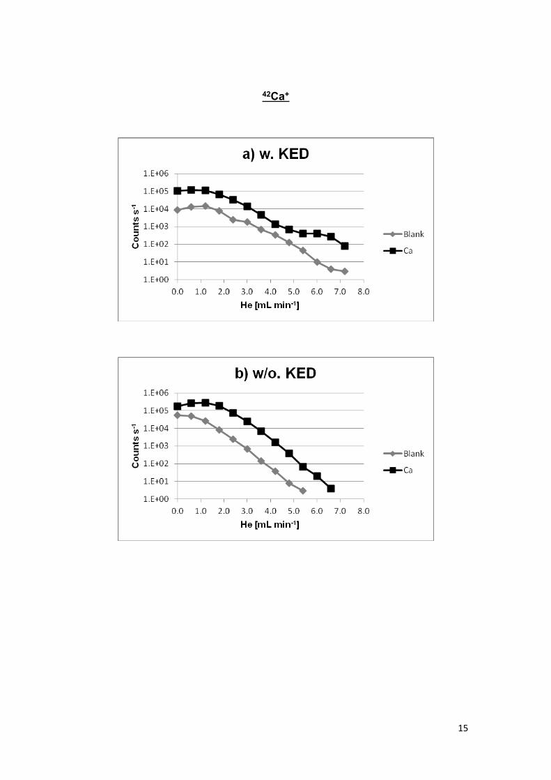
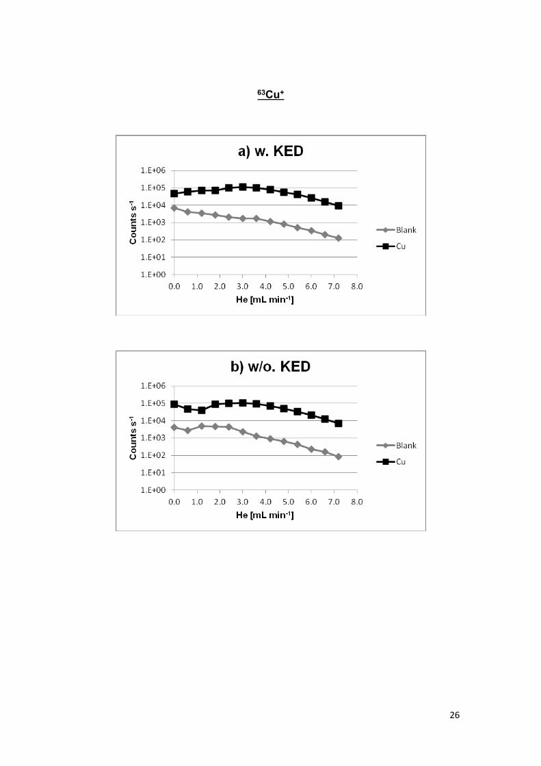
Fig.S5. Signal intensities of all elements and their interferences (blank) as a function of He flow rate: a) w. KED and b) w/o. KED.
24Mg+
14
27Al+
15
42Ca+
16
43Ca+
17
47Ti+
18
51V+
19
52Cr+
20
53Cr+
21
55Mn+
22
56Fe+
23
57Fe+
24
59Co+
25
60Ni+
26
63Cu+
27
65Cu+
28
66Zn+
29
75As+
30
78Se+
31
80Se+
32
88Sr+
33
93Nb+
34
95Mo+
35
107Ag+
36
121Sb+
37
133Cs+
38
137Ba+
39
Fig.S6. Signal intensities of all elements and their interferences (blank) as a function of H2 flow rate: a) w. KED and b) w/o. KED.
24Mg+
40
27Al+
41
42Ca+
42
43Ca+
43
47Ti+
44
51V+
45
52Cr+
46
53Cr+
47
55Mn+
48
56Fe+
49
57Fe+
50
59Co+
51
60Ni+
52
63Cu+
53
65Cu+
54
66Zn+
55
75As+
56
78Se+
57
80Se+
58
88Sr+
59
93Nb+
60
95Mo+
61
107Ag+
62
121Sb+
63
133Cs+
64
137Ba+
65
Table S5 Stopping curves results of He gas flow rate
2.5 mL min-1 He 4.5 mL min-1 HeEin (eV) Eloss(eV) Eout (eV) σΧ/σNi Eloss(eV) Eout (eV) σΧ/σNi