ELECTROSTATIC DENSITY MEASUREMENTS IN GREEN-STATE PM PARTS by Georg H. W. Leuenberger A Dissertation Submitted to the Faculty of the WORCESTER POLYTECHNIC INSTITUTE in Partial Fulfillment of the Requirements for the Degree of Doctor of Philosophy in Electrical Engineering by __________________________ April 2003 APPROVED: Professor Reinhold Ludwig, Major Advisor Professor Robert A. Peura Professor Diran Apelian Professor John M. Sullivan, Jr. Professor William R. Michalson Professor John Orr, ECE Department Head
Transcript
ELECTROSTATIC DENSITY MEASUREMENTS IN GREEN-STATE PM PARTS
by
Georg H. W. Leuenberger
A Dissertation
Submitted to the Faculty
of the
WORCESTER POLYTECHNIC INSTITUTE
in Partial Fulfillment of the Requirements for the
Degree of Doctor of Philosophy
in
Electrical Engineering
by
__________________________
April 2003
APPROVED:
Professor Reinhold Ludwig, Major Advisor
Professor Robert A. Peura
Professor Diran Apelian
Professor John M. Sullivan, Jr.
Professor William R. Michalson
Professor John Orr, ECE Department Head
Abstract
i
Abstract
The goal of this research is to show the feasibility of detecting density variations in green-
state powder metallurgy (P/M) compacts from surface voltage measurements. By monitoring a
steady electric current flow through the sample and recording the voltages over the surface, valu-
able information is gathered leading to the prediction of the structural health of the compacts.
Unlike prior research that concentrated on the detection of surface-breaking and subsurface de-
fects, the results presented in this thesis target the density prediction throughout the volume of
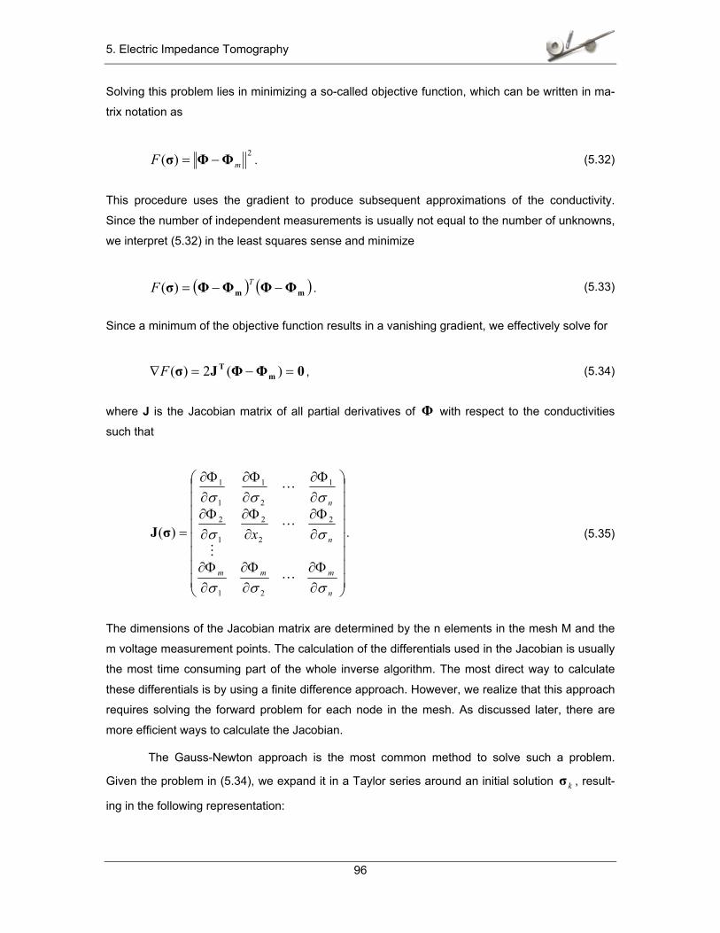
the sample. The detection of density variations is achieved by establishing a correlation between
the conductivity and their respective density. The data obtained from the surface measurements
is used as part of an inversion algorithm, calculating the conductivity distribution, and subse-
quently the density within the compact.
In a first step, the relationship between conductivity and density of green-state P/M com-
pacts was investigated. Tests were conducted for a number of parts of various powder mixtures.
In all cases a clear correlation between conductivity and density could be established, indicating
that measurements of electric conductivity could indeed be exploited in an effort to render valid
information about the density of the sample under test. We found a linear correlation for non-
lubricated parts and a non-linear behavior for lubricated samples. Specifically, it was found that
the conductivity increases with increasing density only up to a maximum value obtained at ap-
proximately 6.9g/cm3. Interestingly, any additional density increase leads to a reduction of the
conductivity. This behavior was confirmed to be inherent in all powder mixtures with lubricants.
The thesis research is able to provide a physical model and a mathematical formulation describ-
ing this counter-intuitive phenomenon.
A finite element solver in conjunction with an inversion algorithm was then implemented
to study arbitrarily shaped part geometries. Based on the principles of electric impedance imag-
ing, the developed algorithm faithfully reconstructs the density distribution from surface voltage
measurements.
The feasibility of the instrumentation approach for both simple and complex parts can be
demonstrated using a new sensor concept and measurement arrangement. Measurements were
performed on both geometrically simple and complex parts.
Acknowledgments
ii
Acknowledgments
This dissertation would not have been possible without the help and support from many
people. My heart felt appreciation goes to my advisor Reinhold Ludwig, whose enthusiasm for
scientific research and the exploration of new areas was a great inspiration during all my work.
His guidance and support helped me through all the problems that arose along the way.
Special thanks go to Diran Apelian and the members of the Powder Metal Research Cen-
ter, who supported my work in numerous ways. Especially the members of the focus group con-
tributed greatly through many helpful, constructive discussions. Also they provided special P/M
samples for my research and helped with the development of sensors. I am grateful for the finan-
cial support I received from the PMRC.
My thanks go to Bill Michalson, Bob Peura and John Sullivan for serving on my commit-
tee and for their constructive comments that helped improve my dissertation.
In addition, I would like to thank all my friends and colleagues at the RF lab and through-
out the department for making this time enjoyable and memorable.
And I want to thank “the women behind the man”. Without the continued support of my
two daughters Sara and Laura and my wife Bea, this whole adventure would never have been
possible. Thank you for believing in me!
Table of Contents
iii
Table of Contents
1 Problem Statement ................................................................................................................. 1 1.1. Goals and Objectives...................................................................................................... 1 1.2. Approach ........................................................................................................................ 2 1.3. Organization ................................................................................................................... 3
2 Introduction to Powder Metallurgy........................................................................................ 5 2.1. The Powder Metallurgy Industry..................................................................................... 5
2.2. Nondestructive Evaluation of P/M Parts ....................................................................... 12 2.2.1. Eddy Current Testing ........................................................................................ 14 2.2.2. Ultrasonic Inspection......................................................................................... 15 2.2.3. X-Ray Inspection............................................................................................... 16 2.2.4. Thermal Imaging ............................................................................................... 16 2.2.5. Electrical Resistivity Inspection......................................................................... 17 2.2.6. Other Techniques ............................................................................................. 20
2.3. Density Measurements in P/M Compacts .................................................................... 21
3 Current Flow in 2 and 3 Dimensions................................................................................... 23 3.1. Two Dimensional Current Flow .................................................................................... 24 3.2. Three Dimensional Current Flow.................................................................................. 30
3.2.1. Basic equations................................................................................................. 30 3.2.2. Current flow through a three-dimensional cylinder ........................................... 35 3.2.3. Numerical predictions ....................................................................................... 35 3.2.4. Comparison with Measurements ...................................................................... 39
4 Conductivity-Density Relationship ..................................................................................... 42 4.1. Measurements on Green P/M Samples ....................................................................... 42
4.2. Conductivity of Mixtures................................................................................................ 54 4.2.1. Non-Conducting Particles in Conducting Medium ............................................ 54 4.2.2. Depolarization Effect......................................................................................... 61
4.3. Conductivity-Density Relationship for Green P/M Samples ......................................... 65
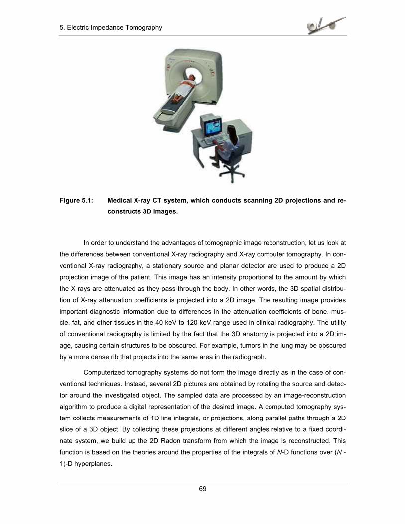
5 Electric Impedance Tomography ........................................................................................ 68 5.1. Introduction ................................................................................................................... 68
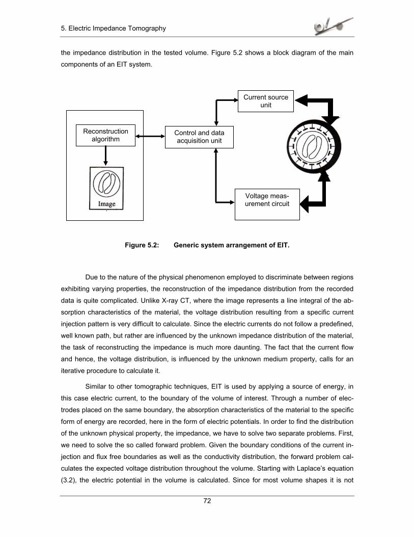
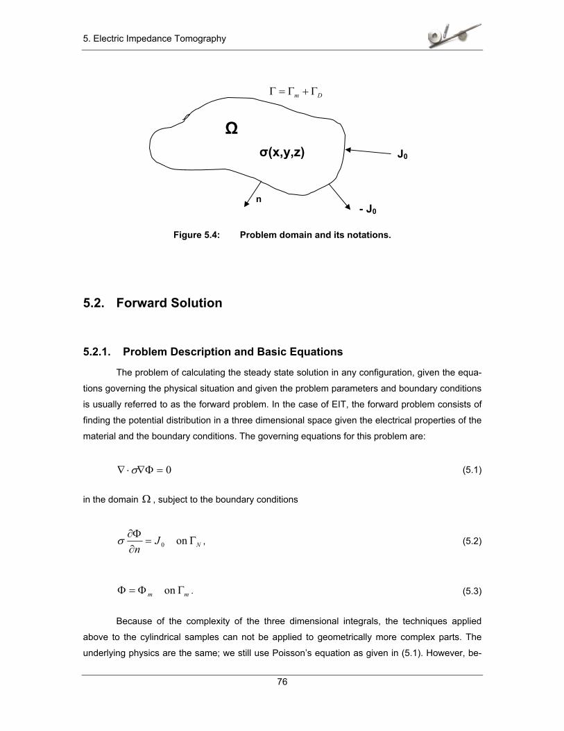
5.1.1. Definition of Tomography.................................................................................. 68 5.1.2. Principles of Electric Impedance Tomography ................................................. 70 5.1.3. Applications....................................................................................................... 74 5.1.4. Notation............................................................................................................. 75
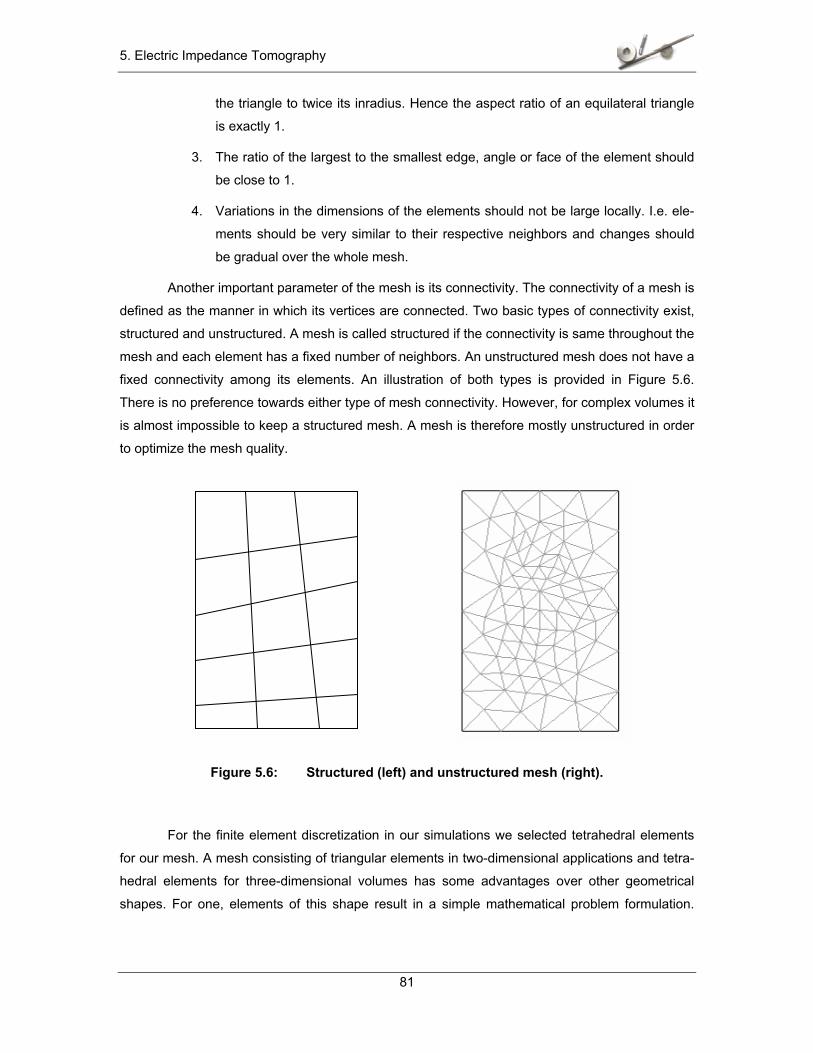
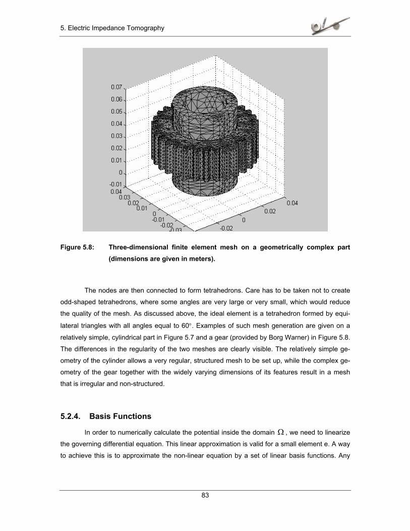
5.2. Forward Solution........................................................................................................... 76 5.2.1. Problem Description and Basic Equations........................................................ 76 5.2.2. Discretization..................................................................................................... 77 5.2.3. Mesh Generation .............................................................................................. 79 5.2.4. Basis Functions................................................................................................. 83 5.2.5. Finite Element Solution ..................................................................................... 86
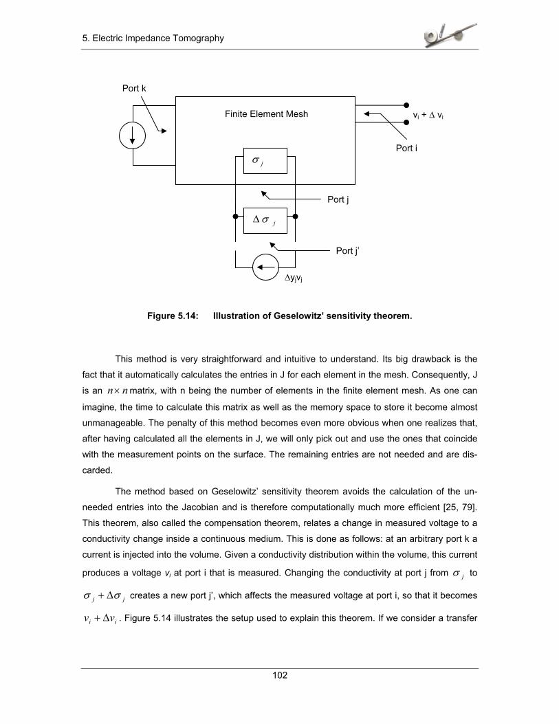
5.3. Inverse Algorithm.......................................................................................................... 93 5.3.1. Problem Statement ........................................................................................... 93 5.3.2. Approach........................................................................................................... 93 5.3.3. Underdetermined versus Overdetermined Problems ....................................... 97 5.3.4. Regularization and Use of a Priori Information................................................. 98 5.3.5. Efficient Calculation of Jacobian..................................................................... 100
5.4. Application of EIT to P/M parts ................................................................................... 105
6 Density Measurements....................................................................................................... 107 6.1. Algorithm..................................................................................................................... 107 6.2. Measurements on Simple Parts ................................................................................. 108
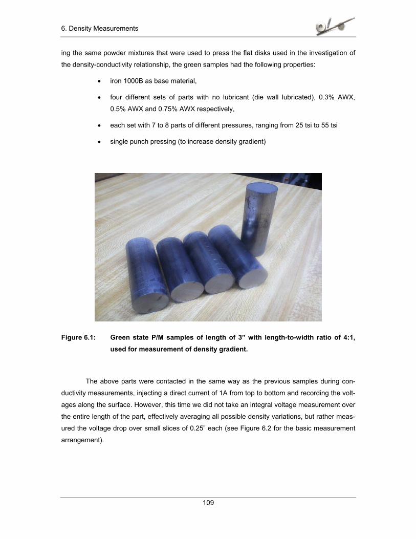
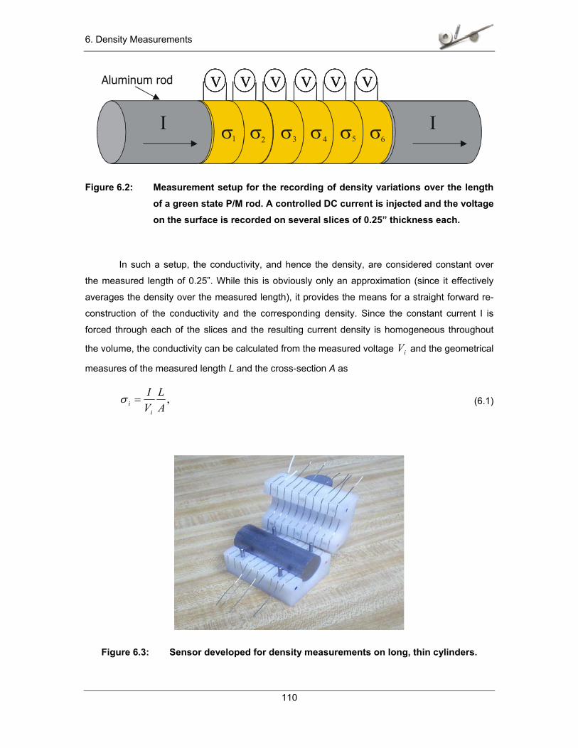
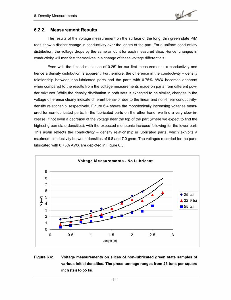
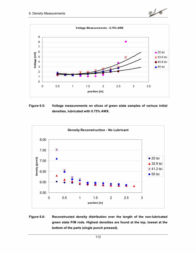
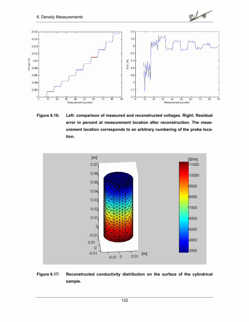
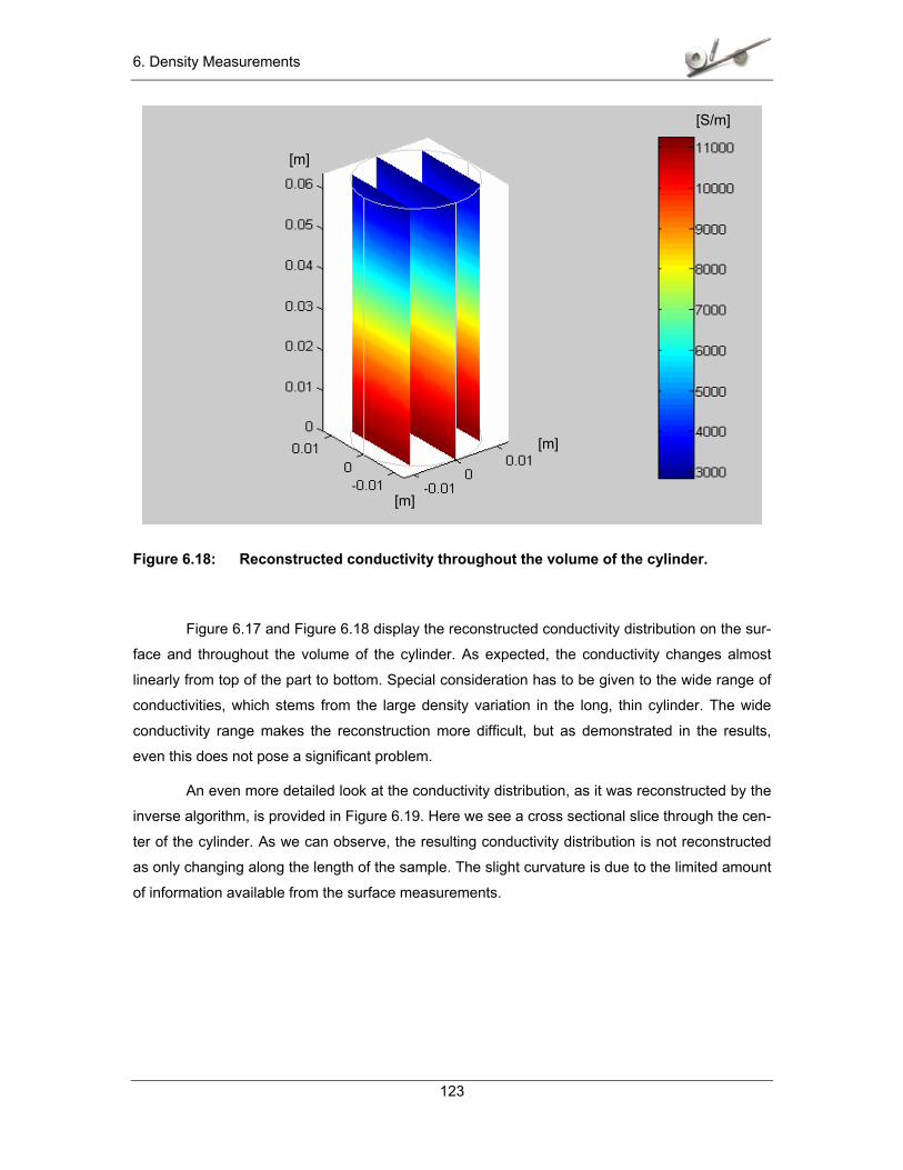
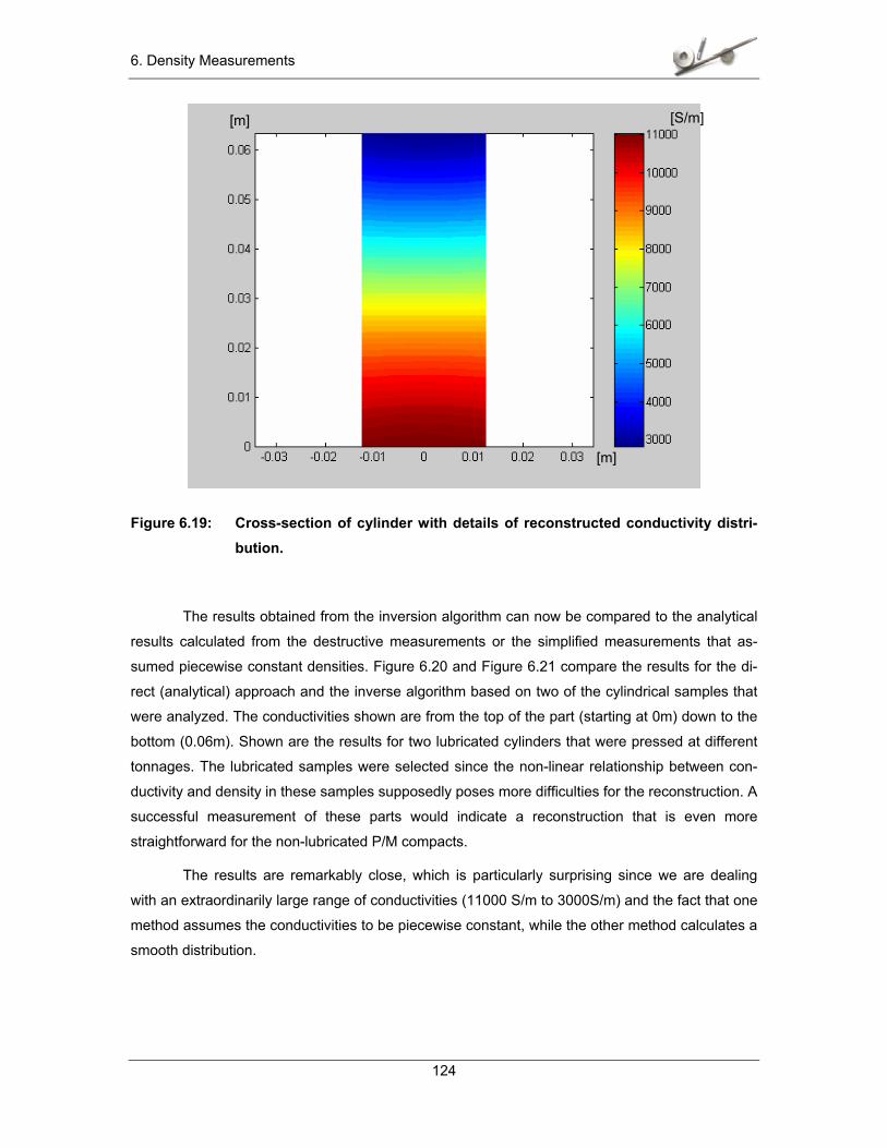
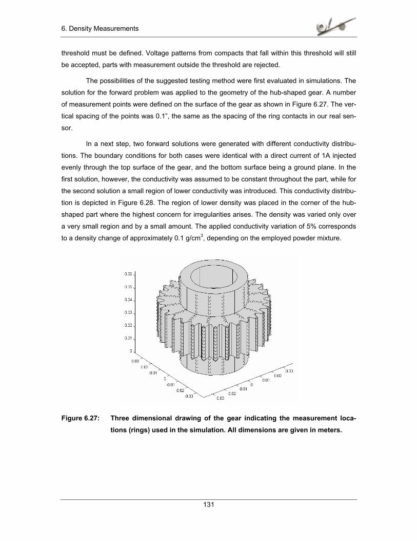
6.2.1. Parts and Measurement Setup for Density-Reconstruction ........................... 108 6.2.2. Measurement Results ..................................................................................... 111 6.2.3. Comparison with Conventional Methods ........................................................ 114 6.2.4. Density Measurements with EIT Algorithm..................................................... 120
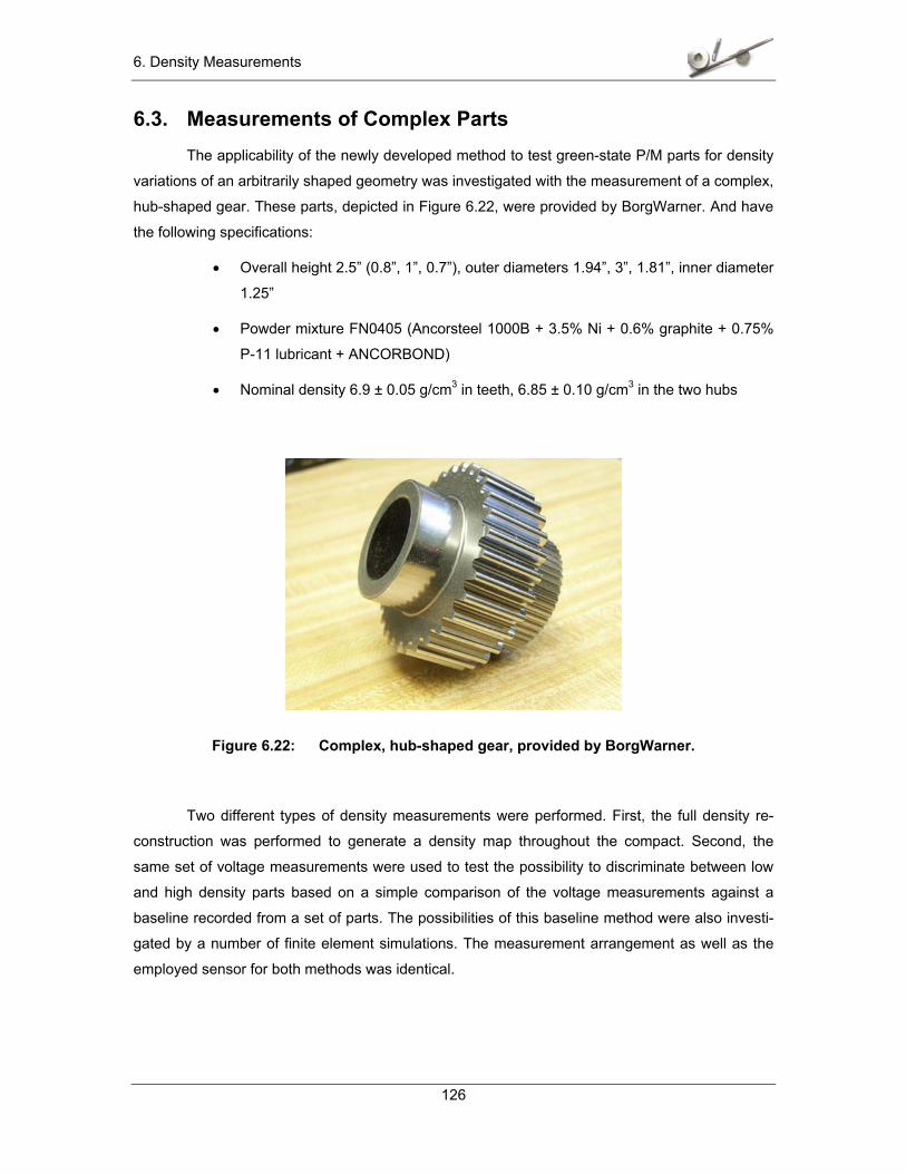
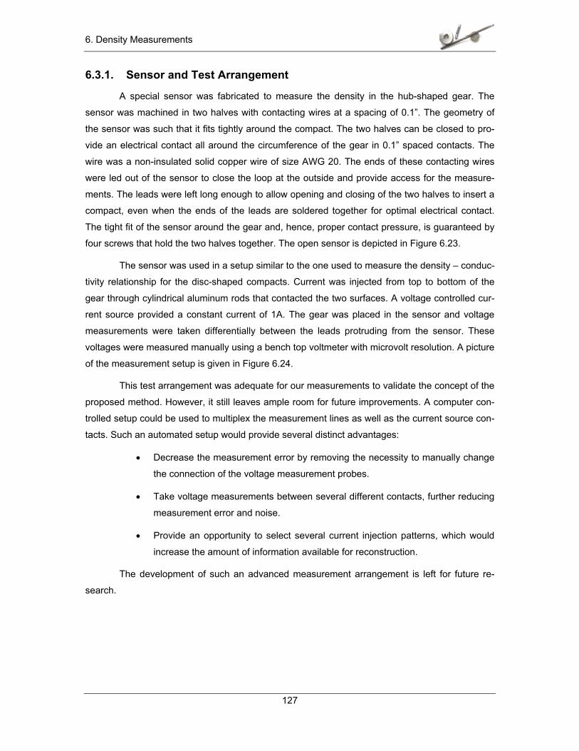
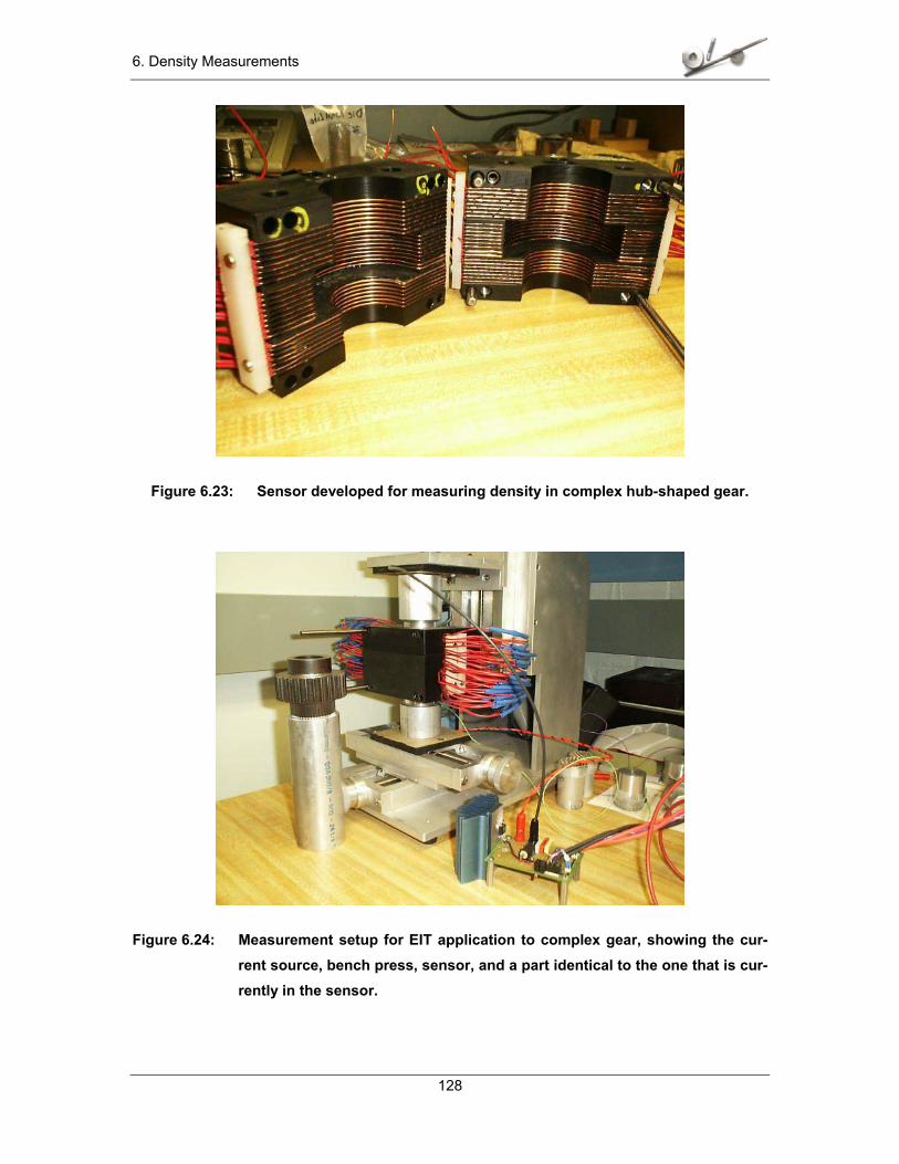
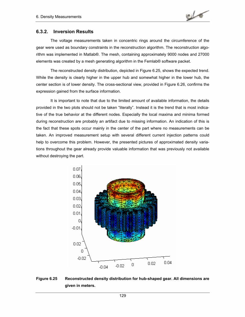
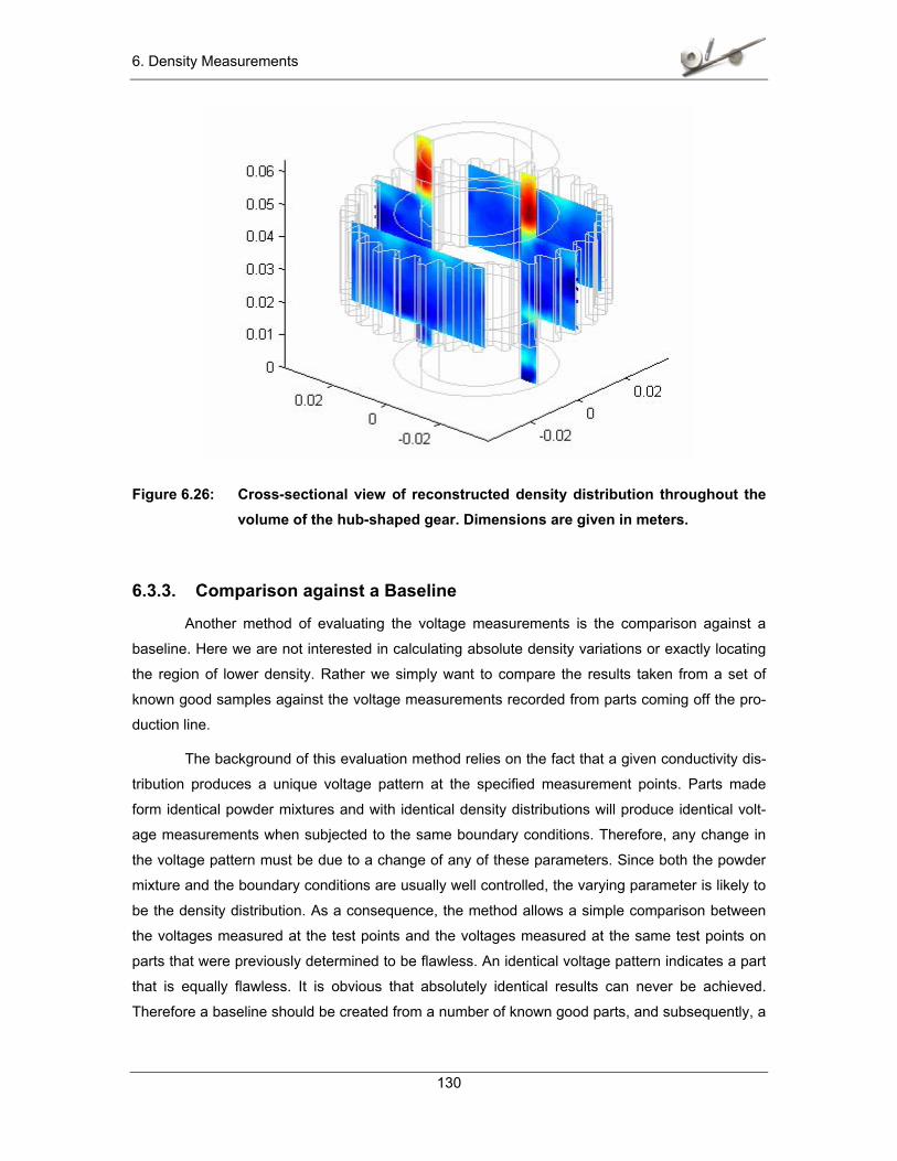
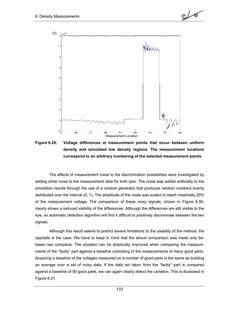
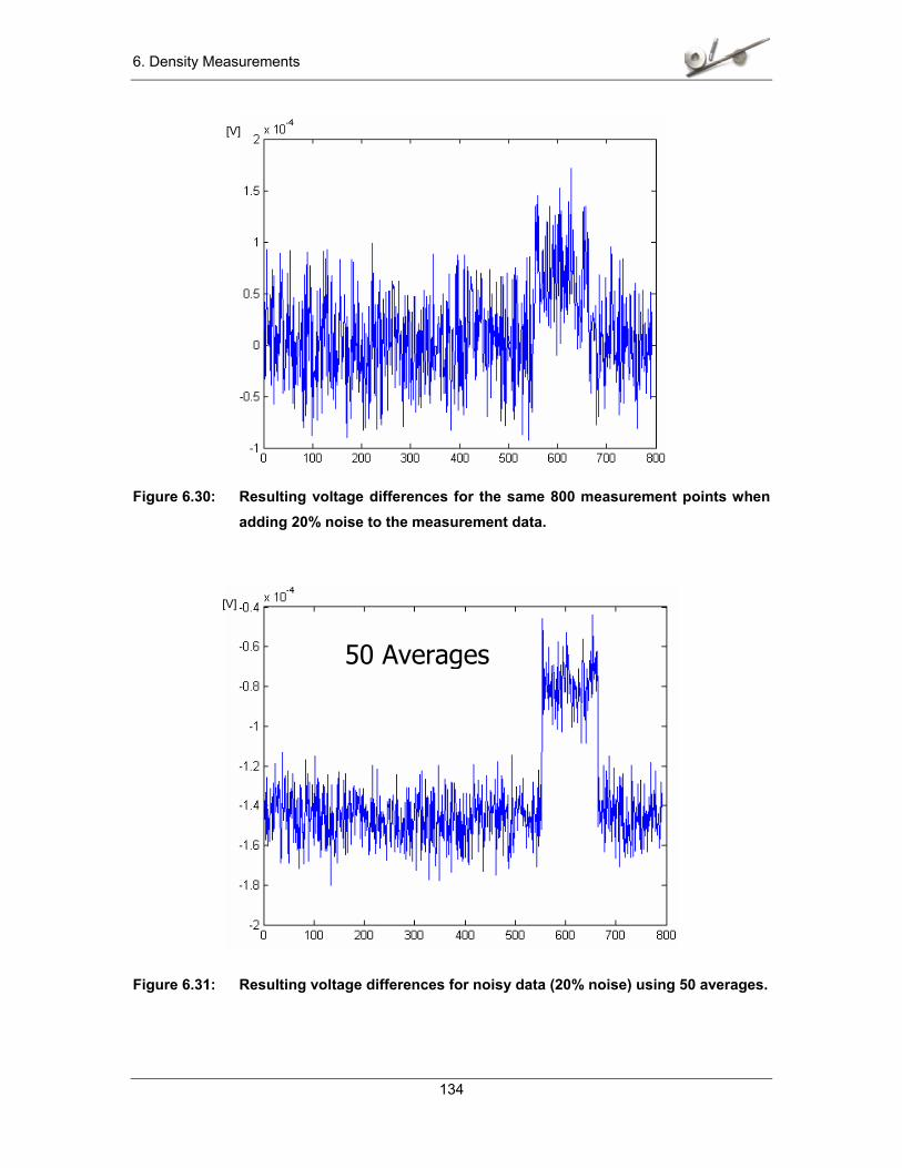
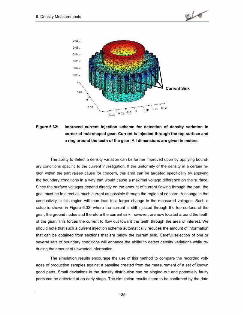
6.3. Measurements on Complex Parts .............................................................................. 126 6.3.1. Sensor and Test Arrangement........................................................................ 127 6.3.2. Inversion Results ............................................................................................ 129 6.3.3. Comparison against a Baseline ...................................................................... 130
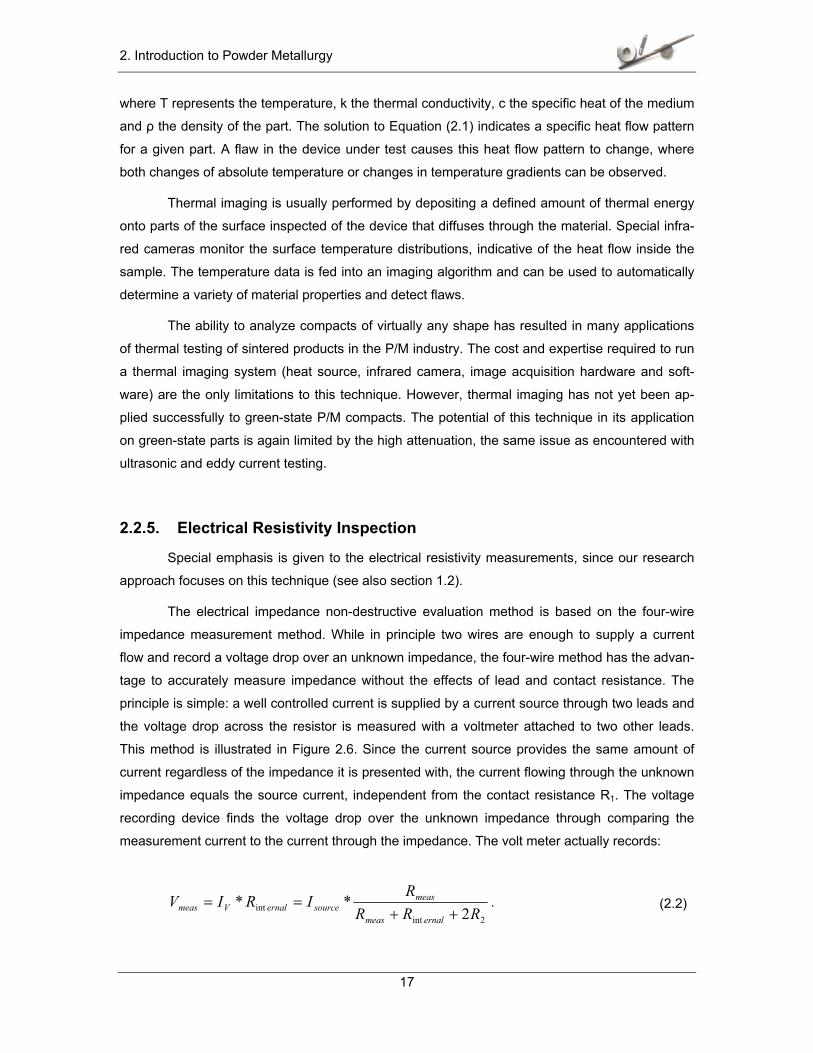
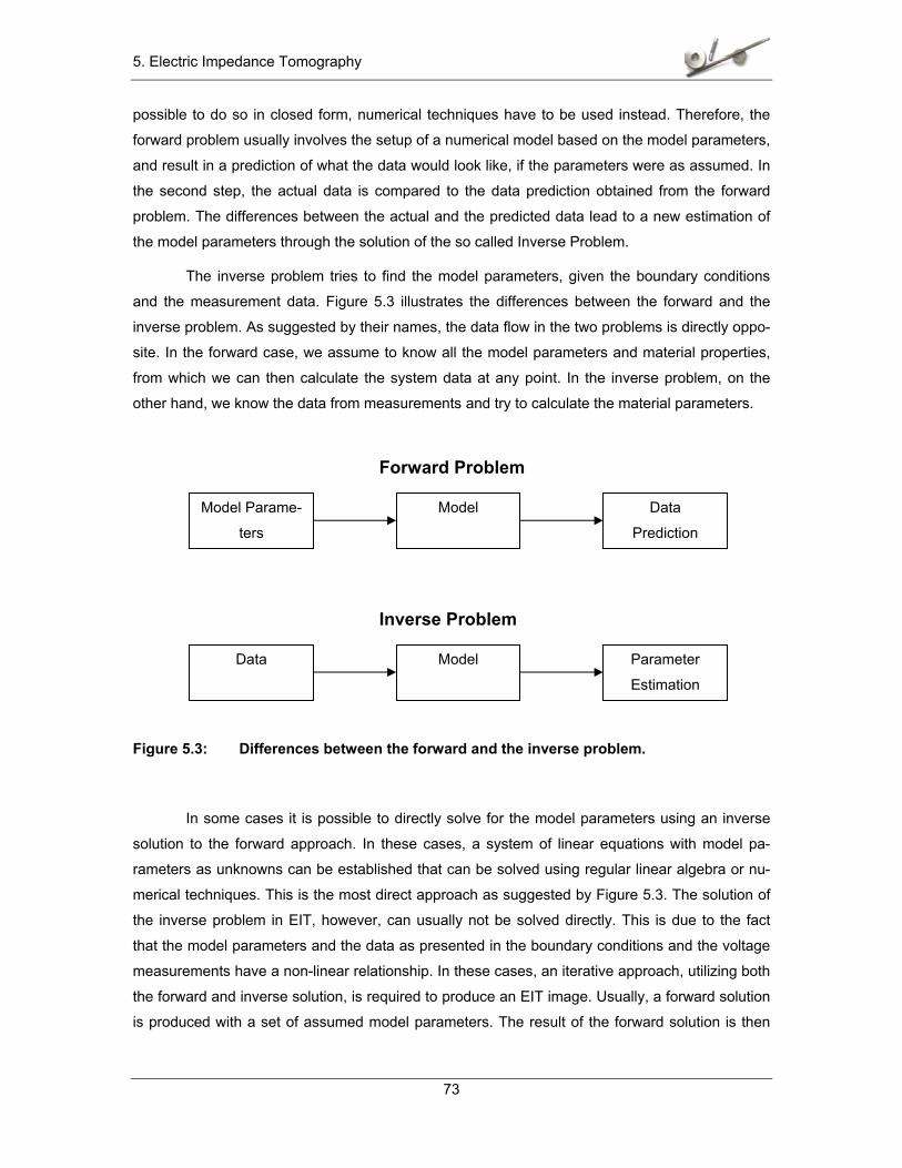
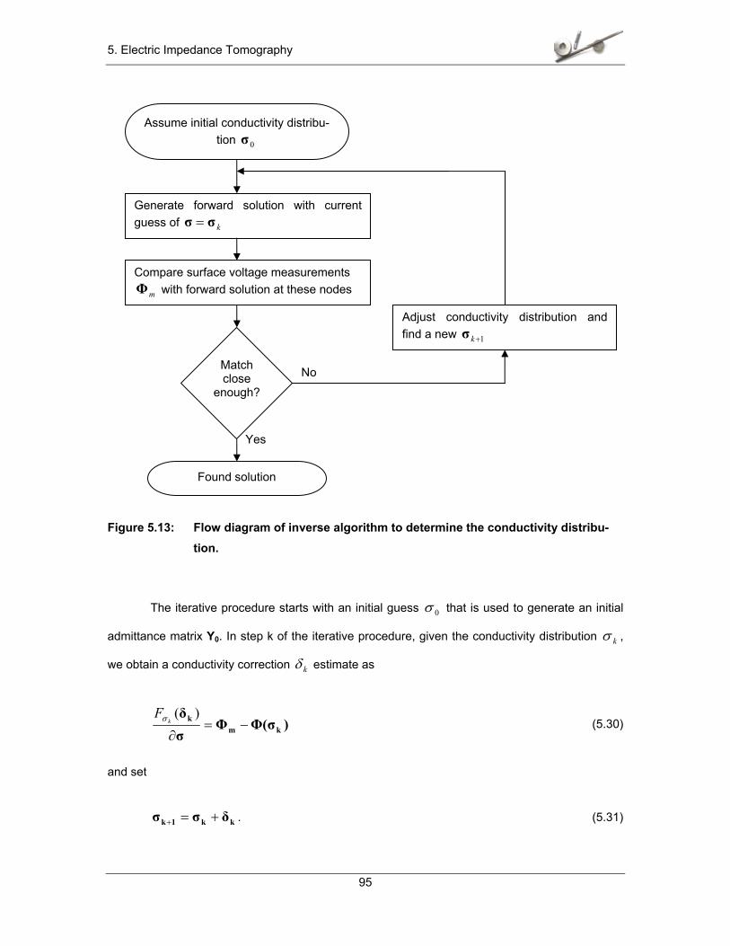
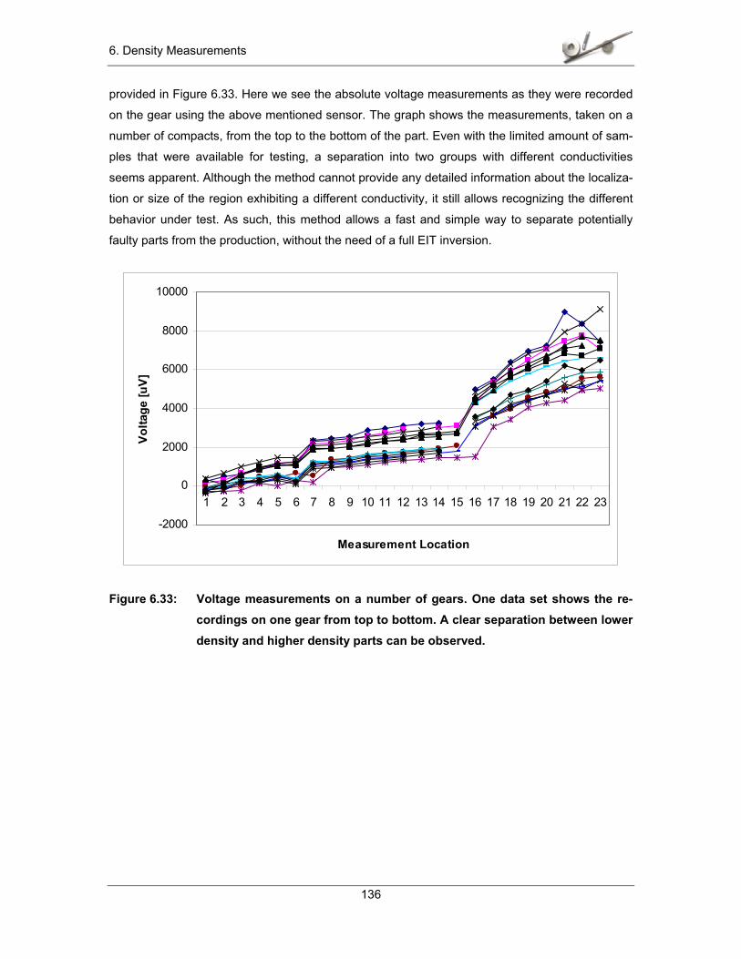
In this arrangement, the relationship between the measurements and the material con-
ductivity is more complicated and can no longer be approximated by the ratio of current and volt-
age. Since we cannot assume the direction and the density of the current throughout the material
to be constant, the geometry of the part has to be taken into consideration. If the solid is large
enough so that we can assume it to extend to infinity with respect to the dimensions of the probe
VMeasured Impedance Current
Source Volt- meter
Iv ≈ 0
Isource
Contact and lead resistances
R2
R2
R1
R1
Rmeas
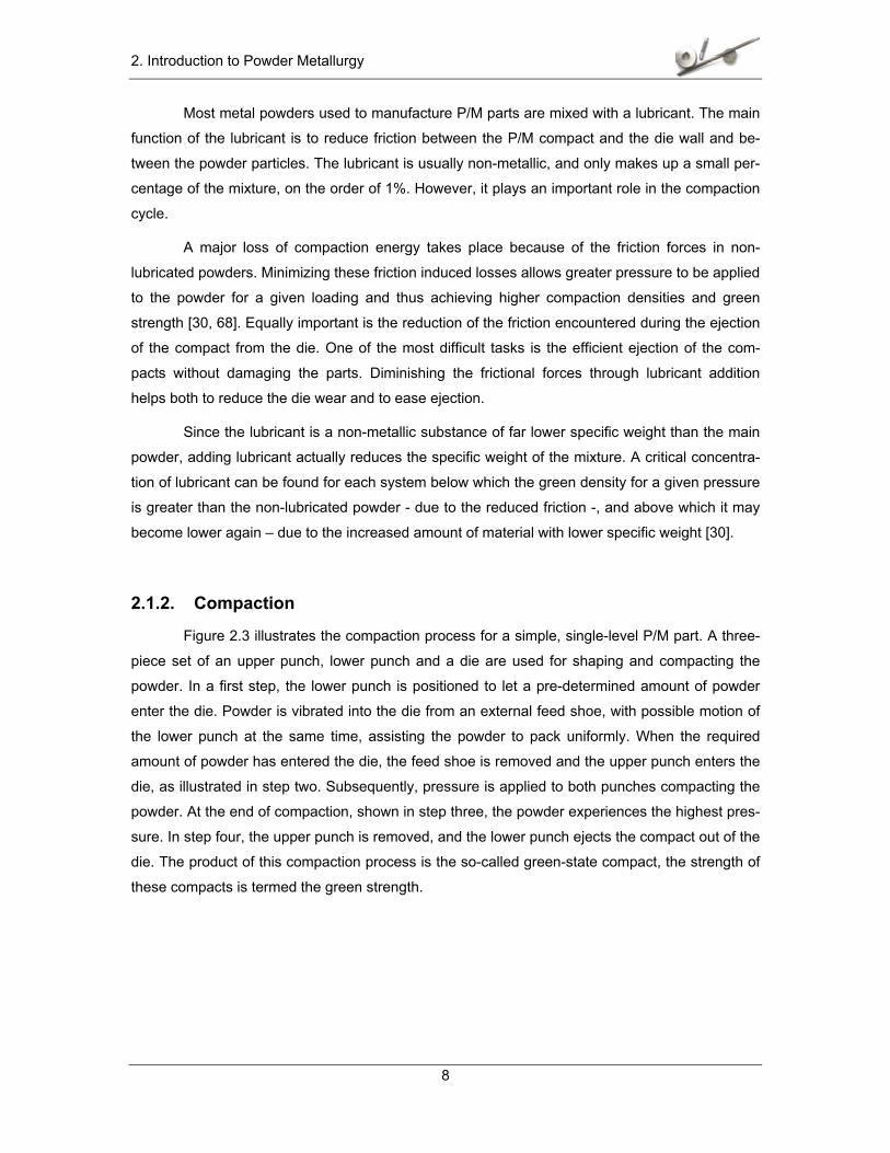
2. Introduction to Powder Metallurgy
19
placement, then boundary effects can be neglected and the underlying Laplace equation can be
solved by modeling the solid as a half-space. In this simplified geometry, the relationship between
the unknown conductivity σ, the injected current and the recorded voltage is given by:
−−
−=
4321
11112 rrrrVIπ
σ . (2.3)
Equation (2.3) is an analytical solution of the current flow in a uniform conducting half-
space [9]. If the material is relatively thin and the effects of current flow extending to the edge of
the material have to be taken into consideration – as is the case in a sheet of metal - the material
thickness enters the equation as a correction factor [44].
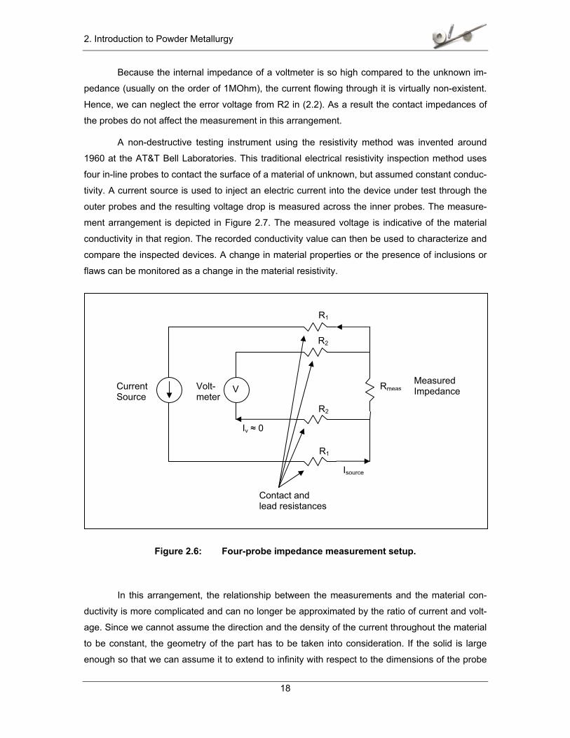
Figure 2.7: Four-probe setup for resistivity measurement [9].
In P/M compacts, resistivity is a good indicator of material properties. The technique can
be used on both sintered and green-state parts. Its application is not limited by properties specific
to P/M compacts but rather by the limitations of the technique itself. Since current cannot be di-
rected within the part but rather distributes according to the physical laws, the resolution and the
application to specific areas of interest are limited. Nevertheless, successful implementations
Current source
Voltmeter
r1 r2
r3 r4
2. Introduction to Powder Metallurgy
20
have shown the technique’s value especially in the detection of surface and near sub-surface
flaws. When a flaw is present between the voltage probes, the resistivity reading will be higher
than normal and the flaw can be detected.
Several versions of this method have been investigated in recent years. The traditional
four-probe inline resistivity inspection as developed by AT&T has two main disadvantages. First,
the sensor must be moved across the entire surface of the part, rendering the inspection very
slow. Second, the spacing of the probes allows only to either increase the resolution by placing
the probes close together, or increasing the ability to detect deep subsurface flaws, but not both
at the same time.
These limitations have been addressed by an apparatus for crack detection in green-
state P/M compacts developed at Worcester Polytechnic Institute [8, 71]. This crack detection
system extends the four-probe approach by applying a grid of spring loaded needle contacts to
the surface of the tested part. While current is still injected through two of the contacts, a large
number of differential voltages are recorded between the remaining probes covering the part un-
der test. It is the voltage distribution that is subsequently processed in a signal processing algo-
rithm and results in the detection and location of surface and sub-surface flaws. Flaws caused a
perturbation in the voltage signals when compared to flawless samples, and this perturbation can
be detected using a statistical algorithm [9].
2.2.6. Other Techniques
Numerous other techniques have been invented to inspect P/M products. Some of these
techniques are named in the following list:
• Resonance frequency testing
• Magnetic particle inspection
• Liquid penetration measurement
Each technique finds a specialized application and supporters for certain cases. All of
them have only limited application, if any at all, regarding the inspection of green-state P/M parts.
The special composition of the green-state samples with respect to their amorphous structure,
their low mechanical strength and high attenuation provides insurmountable obstacles for the
successful application for all of these techniques.
2. Introduction to Powder Metallurgy
21
2.3. Density Measurements in P/M Compacts Density measurements have a special importance in P/M produced parts. The many rea-
sons for this are rather obvious. Since P/M compacts are produced from a powder, the density of
the part promises direct characterization of the powder purity, the quality of the filling and com-
pacting processes, and , ultimately, of the mechanical strength of the final product. Hence most
P/M component properties are closely related to the final density.
The density of P/M compacts can be expressed in two ways. It can be either recorded in
the regular units of weight per unit volume, usually in g/cm3, or it can also be expressed as per-
cent of theoretical density, which is the ratio of the density of the P/M component to that of its cast
metal counterpart. This measure gives direct information about the remaining porosity of the part,
where a part with 85% theoretical density is said to have a porosity of 15%.
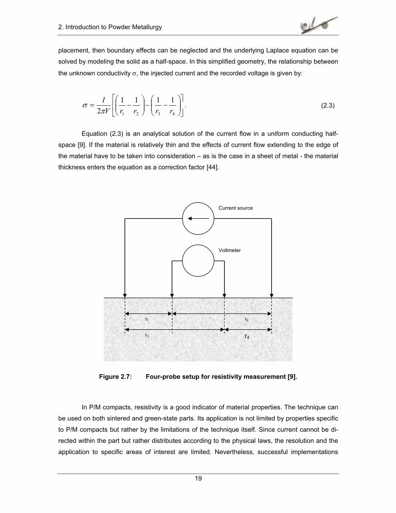
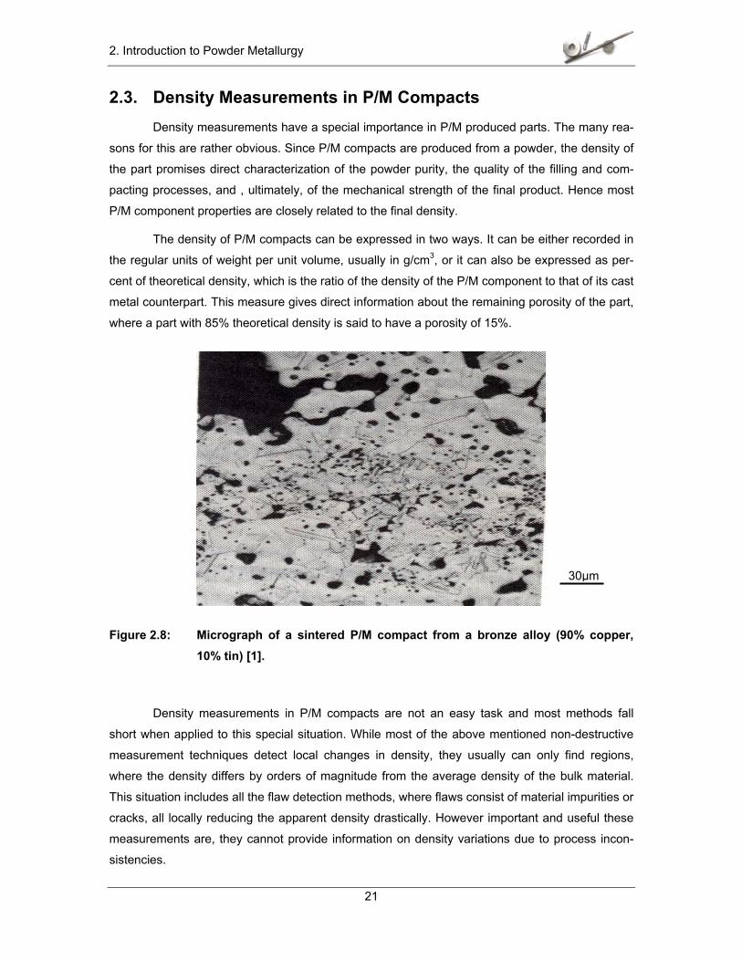
Figure 2.8: Micrograph of a sintered P/M compact from a bronze alloy (90% copper, 10% tin) [1].
Density measurements in P/M compacts are not an easy task and most methods fall
short when applied to this special situation. While most of the above mentioned non-destructive
measurement techniques detect local changes in density, they usually can only find regions,
where the density differs by orders of magnitude from the average density of the bulk material.
This situation includes all the flaw detection methods, where flaws consist of material impurities or
cracks, all locally reducing the apparent density drastically. However important and useful these
measurements are, they cannot provide information on density variations due to process incon-
sistencies.
30µm
2. Introduction to Powder Metallurgy
22
Apart from the very local density measurements that enable the detection of inclusions or
cracks, all other non-destructive techniques available today only allow to measure an average
density for the whole part. This means that they simply measure the weight and the part dimen-
sions, and from that calculate the average density. The only method that allows measuring a
density distribution within the P/M part, in both the green and sintered state, is by micrographs. In
this method, the part is cut into several thin slices that subsequently are analyzed under the mi-
croscope. By measuring the area of the pores compared to the area of the metallic material, a
local density can be calculated. Figure 2.8 shows such a micrograph for a sintered bronze alloy,
where the remaining pores are clearly visible.
3. Current Flow in 2 and 3 Dimensions
23
3 Current Flow in 2 and 3 Dimensions
An important step toward understanding the results from voltage measurements on a
conductive part is the insight into the flow of electric current in two and three dimensions. In many
cases one is only concerned about the macroscopic view of current flowing through an imped-
ance. In such a case we are not concerned about the direction of the current flow, but merely as-
sume a uniform current density throughout the volume, with the current flowing from higher to
lower potential. In the case of DC current, this behavior can be mathematically described by the
relationship of voltage and current over a resistor:
IRV = , (3.1)
where R is the lumped resistance value, I is the current flowing through the part and V is the re-
sulting drop in potential.
This simplified view, however, does no longer apply to a scenario, where current is in-
jected into a part through contacts, whose surfaces are small compared to the measured part,
and where voltages are measured in several positions on the surface. In order to calculate the
voltage distribution and the current flow within the measured part, we now have to find a solution
to Laplace’s equation
0=Φ∇⋅∇ σ , (3.2)
given the boundary conditions of the injected current density at defined locations on the boundary
of the part. In general, we have to assume a non-uniform conductivity in the sample. This spatial
dependency of the conductivity makes both ),,( zyxσσ = and ),,( zyxΦ=Φ a function of the
spatial coordinates x, y, z. In the case of a uniform conductivity, (3.2) reduces to
02 =Φ∇ . (3.3)
3. Current Flow in 2 and 3 Dimensions
24
Generally, a closed form solution for (3.2) cannot be found. In some cases, where the geometry is
such that a closed solution to the resulting integrals can be found, the flow of the current and the
resulting voltage distribution can be determined anywhere in the geometry. The following para-
graphs go through a two-dimensional and a three-dimensional case that are both of interest to
our research.
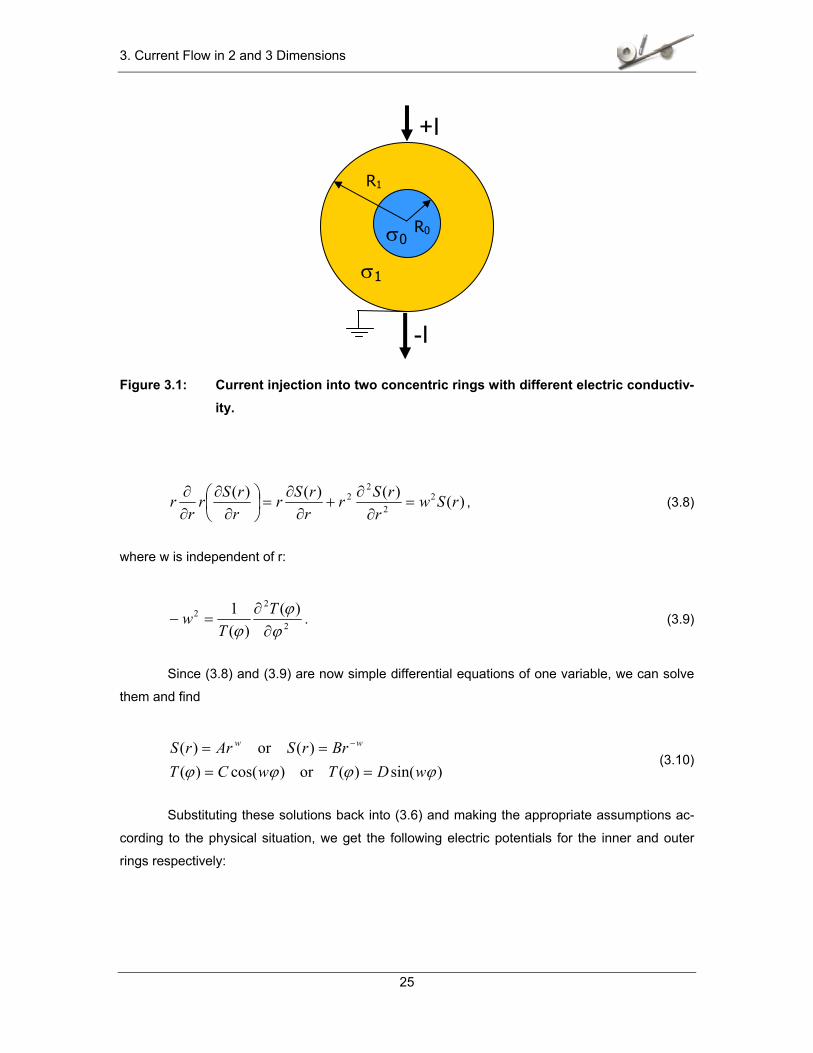
3.1. Two Dimensional Current Flow Let us consider two concentrical circular regions of conductive materials as shown in
Figure 3.1. The inner circular area has a radius R0 and conductivity σ0, the outer ring has a radius
R1 and conductivity σ1. A current I of strength I0 is applied to this part through point contacts at
the angular position 0=ϕ and a current sink of equal magnitude at position πϕ = , so that
))()((0 πξδξδ −−= II , (3.4)
In order to find the steady state voltage distribution and current flow pattern in this circular
region, we need to solve Equation (3.2). Rewriting (3.2) in polar coordinates, we get:
01)(12
2
2 =∂Φ∂
+∂Φ∂
∂∂
ϕrrr
rr. (3.5)
Using the method of the separation of variables, we separate the dependence of Φ on r
and φ into two separate functions, each depending on only one of the two independent variables:
)()(),( ϕϕ TrSr =Φ . (3.6)
Using these variable separated functions, (3.5) becomes
0)()(
1)()( 2
2
=∂
∂+
∂∂
∂∂
ϕϕ
ϕT
TrrSr
rrSr
. (3.7)
Equation (3.7) can now be solved for S(r) and T(φ) independently as we can write
3. Current Flow in 2 and 3 Dimensions
25
Figure 3.1: Current injection into two concentric rings with different electric conductiv-ity.
)()()()( 22
22 rSw
rrSr
rrSr
rrSr
rr =
∂∂
+∂
∂=
∂∂
∂∂
, (3.8)
where w is independent of r:
2
22 )(
)(1
ϕϕ
ϕ ∂∂
=−T
Tw . (3.9)
Since (3.8) and (3.9) are now simple differential equations of one variable, we can solve
them and find
)sin()(or)cos()()(or)(
ϕϕϕϕ wDTwCTBrrSArrS ww
==== −
(3.10)
Substituting these solutions back into (3.6) and making the appropriate assumptions ac-
cording to the physical situation, we get the following electric potentials for the inner and outer
rings respectively:
+I
-I
σ1
R1
σ0R0
3. Current Flow in 2 and 3 Dimensions
26
( ) )cos(),(
)cos(),(
1
0
ϕϕ
ϕϕ
nCrBrr
nArrnn
n
−+=Φ
=Φ (3.11)
The unknown constants A, B, and C can now be calculated by taking into account the
proper boundary conditions of the problem. In words, these boundary conditions can be stated as
follows:
• The potential at the inner boundary between the two areas must be continuous.
• The current flow at this inner boundary must be the same in both regions.
• The current flow at the outer boundary is defined by the two points of the current
source and the current sink.
Additionally, the potential was fixed to 0 at the current sink location. This convention is
arbitrary, but we need to fix the potential at one point in the volume to make the solution unique.
Mathematically, these boundary conditions allow us to setup up the following three equations:
00 10 RrRr == Φ=Φ (3.12)
00
11
00 RrRr rr == ∂
Φ∂=
∂Φ∂
σσ (3.13)
),(1
11 ϕσ rIr Rr =∂Φ∂
= (3.14)
Using (3.12), (3.13), and (3.14) to evaluate the proportionality constants, we find for the
potential in the region of interest
≥≥+−
≤−=Φ
∑
∑∞
=
−
∞
=
01,...5,3,1
20
0,...5,3,1
,cos)()(
,cos)1()(),(
RrRnrhRrnb
Rrnrhnbr
n
nnn
n
n
ϑ
ϑϑ , (3.15)
where nn
n
hRRR
nI
nbh 20
21
11
2
0
21
21 2)(,
+=
+−
=+
πσσσσσ
.
The series in the solution converges quickly and can be approximated with only a few
terms of the sum. The series was programmed in Matlab® and the results of the simulations are
3. Current Flow in 2 and 3 Dimensions
27
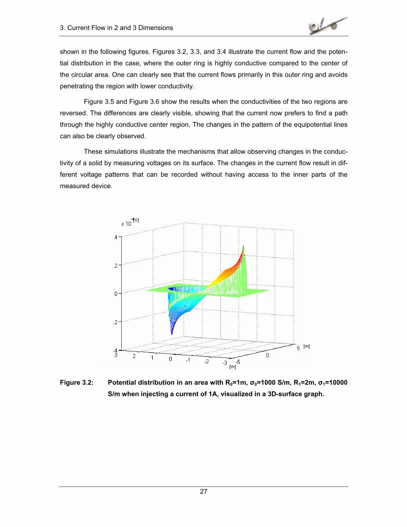
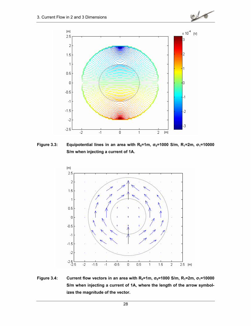
shown in the following figures. Figures 3.2, 3.3, and 3.4 illustrate the current flow and the poten-
tial distribution in the case, where the outer ring is highly conductive compared to the center of
the circular area. One can clearly see that the current flows primarily in this outer ring and avoids
penetrating the region with lower conductivity.
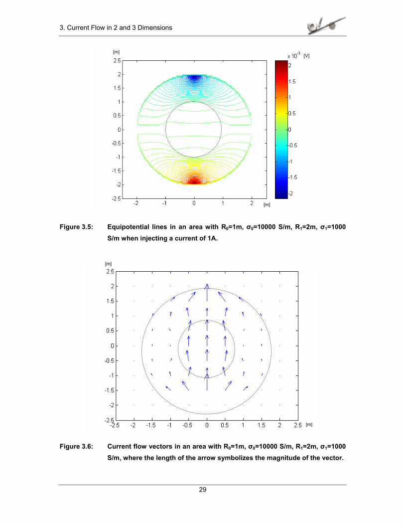
Figure 3.5 and Figure 3.6 show the results when the conductivities of the two regions are
reversed. The differences are clearly visible, showing that the current now prefers to find a path
through the highly conductive center region. The changes in the pattern of the equipotential lines
can also be clearly observed.
These simulations illustrate the mechanisms that allow observing changes in the conduc-
tivity of a solid by measuring voltages on its surface. The changes in the current flow result in dif-
ferent voltage patterns that can be recorded without having access to the inner parts of the
measured device.
Figure 3.2: Potential distribution in an area with R0=1m, σ0=1000 S/m, R1=2m, σ1=10000 S/m when injecting a current of 1A, visualized in a 3D-surface graph.
[V]
[m]
[m]
3. Current Flow in 2 and 3 Dimensions
28
Figure 3.3: Equipotential lines in an area with R0=1m, σ0=1000 S/m, R1=2m, σ1=10000 S/m when injecting a current of 1A.
Figure 3.4: Current flow vectors in an area with R0=1m, σ0=1000 S/m, R1=2m, σ1=10000 S/m when injecting a current of 1A, where the length of the arrow symbol-izes the magnitude of the vector.
[V]
[m]
[m]
[m]
[m]
3. Current Flow in 2 and 3 Dimensions
29
Figure 3.5: Equipotential lines in an area with R0=1m, σ0=10000 S/m, R1=2m, σ1=1000 S/m when injecting a current of 1A.
Figure 3.6: Current flow vectors in an area with R0=1m, σ0=10000 S/m, R1=2m, σ1=1000 S/m, where the length of the arrow symbolizes the magnitude of the vector.
[V]
[m]
[m]
[m]
[m]
3. Current Flow in 2 and 3 Dimensions
30
3.2. Three Dimensional Current Flow
3.2.1. Basic equations
The electric current flow through a P/M compact can be cast in terms of an electrostatic
model formulation of Laplace’s equation whereby the surface currents and voltages represent
boundary conditions, and the conductivity σ is in general spatially non-uniformly distributed
throughout the part. Previously, we assumed the conductivity to be constant in a predefined re-
gion and not vary with location. Generally, this is not true and hence, the voltage Ф(r), as a func-
tion of the spatial observation vector r = r(x,y,z), is therefore given by the generalized Laplace
equation [28]
0)]()([ =Φ∇∇ rrσ . (3.16)
The practically relevant boundary condition involves a prescribed current density input
Φ∇−=∂Φ∂
= σσk
J n (3.17)
(where k denotes the normal vector at the boundary) over an otherwise flux free surface. This
current density is normal to the sample surface whose surface normal k is pointing outwards. An
alternative approach involves Poisson’s equation where the current excitation is incorporated as
part of the right hand side source term
)()]()([ 0rrrr −−=Φ∇∇ δσ I . (3.18)
Here 0r denotes the location of the current source I. and δ is the delta function. Although
the conductivity cannot be regarded as homogeneous throughout the volume, we will for the mo-
ment consider this specialized case, which allows us to simplify Equation (3.19) considerably. For
homogeneously conductive samples Equation (3.18) reduces to
σδϕ /)()( 02 rrr −−=∇ I . (3.19)
To develop a potential solution in a cylindrical (r,θ, z) coordinate system of a sample with
total radius R and length L subject to flux-free (or Neumann-type) boundary condition, we develop
a spectral solution by utilizing eigenfunctions of the form [57, 58]
3. Current Flow in 2 and 3 Dimensions
31
)/cos()cos()/()( LzpmRrJ mnmmnp πθλ=Ψ r . (3.20)
Here )/( RrJ mnm λ is the Bessel function of order m. Index n denotes the zeros of the
first derivative of the Bessel function, i.e. Jm’( mnλ ) = 0, as required to satisfy the flux-free bound-
ary condition. These functions can be expanded as part of a Green’s function expansion [58]
∑∞
+
ΨΨ=
pnm mn
mnpmnp
LpRIG
,,22
00 )/()/(
)()()|(
πλσrr
rr , (3.21)
where the overbar is used to denote an orthonormal set. The function mnpΨ is found by applying
the orthonormality conditions of the Bessel functions mJ [75]
nnmnmmn
R
nmmmnm JmRrdrRrJRrJ ′′
−=∫ δλλ
λλ )(12
)/()/( 22
22
0
, (3.22)
orthogonality of trigonometric functions )cos( θm
∫ ′=′π
επδθθθ2
0
/2)cos()cos( mmmdmm , (3.23)
and orthogonality of trigonometric functions )/cos( Lzpπ
ppp
L
LdxxppxLdzLzpLzp εδππππ /)cos()cos()/'cos()/cos(1
00′=′= ∫∫ , (3.24)
where the primed indices indicate identical functions but with different values of the run-
ning index.
In (3.23) and (3.24) we use the Neumann factor
==
=otherwise,2
001,
p,m,pm εε
This leads to the orthonormal eigenfunctions
3. Current Flow in 2 and 3 Dimensions
32
)()(1
)(2
2
22
rr mnp
mnmmn
pmmnp
JmLRΨ
−
=Ψ
λλ
π
εε. (3.25)
Substituting (3.20) and (3.25) into (3.21) permits us to develop a series expression for the
Green’s function in the form
)]/cos()cos()/(
)/cos()cos()/([)|(
000
0,,0
LpzmRrJ
LpzmRrJGIG
mnm
pnmmnmmnp
πθλ
πθλσ ∑
∞
=
=rr (3.26)
where the coefficient mnpG is a combination of the orthonormality condition (3.25) and the
eigenvalue expression in (3.21). Evaluating the integrals, we explicitly obtain
)(1 22
22
2
2
2
22
mnmmn
mn
pmmnp
JLp
RmLR
Gλπλ
λπ
εε
+
−
= . (3.27)
A simplification of expressions (3.26) and (3.27) can be achieved if the cylinder is axis-
symmetric. Since this implies independence of angle θ, we can re-write (3.26) as
)/cos()/cos()/()|( 00,0
00 LzpLzpRrJGIGpn
nnp ππλσ ∑
∞
==
=rr . (3.28)
where the coefficient Gnp in (3.28) is given by
)(202
22
2
22
nn
pnp
JLp
RLR
Gλπλ
π
ε
+
= . (3.29)
Evaluation of (3.28) is a rapidly converging series, typically requiring fewer than 20 terms
to achieve satisfactory precision.
3. Current Flow in 2 and 3 Dimensions
33
In the above calculations we are considering the source to be a true point source and the
solution presented in (3.28) is strictly speaking only valid for an infinitely small point source. Such
a source cannot be practically implemented. In reality, every source will exhibit some finite con-
tact area, through which the current is flowing into the part. The following paragraphs discuss the
extension of the point source solution to the solution for a source with finite aperture.
Let us consider a ring source with an external radius AR and internal radius BR as seen
in Figure 3.7. According to the superposition principle, we can subdivide our source of finite aper-
ture into small subsections. The effect of each of the sub sources is summed up to give the effect
of the whole source. In (3.26), the term related to the source component is
Figure 3.7: Illustration of ring current source with strength I.
)/cos()cos()/( 000 LpzmRrJ mnm πθλ . (3.30)
Replacing the point source by a number N of sub sources which build the mentioned ring
source, the term in (3.30) becomes
∑=
N
iiiimnm LpzmRrJ
1000 )/cos()cos()/( πθλ , (3.31)
where due to the symmetry in the axis symmetric cylinder only the term depending on r0i truly de-
pends on the actual shape of the source. The other two terms either vanish completely or are
constant with respect to the size of the source. Taking the symmetry and geometric dependen-
cies into account, the term depending on the shape and size of the source reduces to
RB
RA
π)(/ 22
BA RRIAIJ−
==
3. Current Flow in 2 and 3 Dimensions
34
∑=
N
i
imnm Rr
J1
0 )(λ . (3.32)
In the limit ∞→N and representing the position and size of the sub sources in polar
coordinates, (3.32) becomes
( ) ϕρρϕρ
λπ
π
∂∂
− ∫ ∫
A
B
R
Rn
BA Rr
JRR
),(1 00
2
022
. (3.33)
Due to the symmetry the integral over the angle is constant. The remaining integral of the
zero order Bessel function can be evaluated using the identity
( ) )()(2 1
11
21
0
1 aJaaxaxJx −−
−
−− −
Γ=∂∫ νν
ν
νν
ν. (3.34)
Using this integral relationship and adjusting the integration borders to reflect our ring
source dimensions, we find for the integrated source term
( )
−
− RR
JRRR
JRRRR B
nBA
nABA
λλπ 1122
2. (3.35)
This expression can now be used in (3.28) so that the final series for any ring source that
is axis symmetric with the cylinder and lies on its face becomes
( ) ∑∞
==×
−
−=
0,00
110220
)/cos()/cos(
)/(2)|(pn
BnB
AnAnnp
BA LzpLzpRRJR
RRJRRrJG
RRRIG
ππ
λλλ
πσrr . (3.36)
Equation (3.36) is again a fast converging series requiring less than 20 terms to achieve
acceptable precision. Furthermore, additional mathematical manipulations allow reducing the
double series to a single series, so that the calculation becomes even easier. It is worth noting
that the solution presented for a ring source is valid for all possible combinations of source radii, s
long as BA RR > . When 0=BR , the source becomes a disc that is concentric with the cylinder.
In the case 0== BA RR , the source degenerates to a point source and (3.36) becomes the
same as (3.28) for a point source.
3. Current Flow in 2 and 3 Dimensions
35
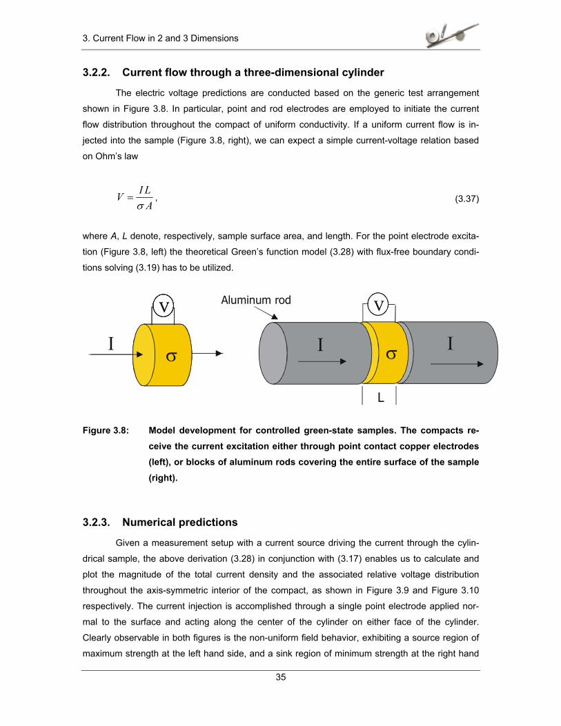
3.2.2. Current flow through a three-dimensional cylinder
The electric voltage predictions are conducted based on the generic test arrangement
shown in Figure 3.8. In particular, point and rod electrodes are employed to initiate the current
flow distribution throughout the compact of uniform conductivity. If a uniform current flow is in-
jected into the sample (Figure 3.8, right), we can expect a simple current-voltage relation based
on Ohm’s law
ALIV
σ= , (3.37)
where A, L denote, respectively, sample surface area, and length. For the point electrode excita-
tion (Figure 3.8, left) the theoretical Green’s function model (3.28) with flux-free boundary condi-
tions solving (3.19) has to be utilized.
σ
VV
I I
Aluminum rod
L
σ
V
I σ
VV
Figure 3.8: Model development for controlled green-state samples. The compacts re-ceive the current excitation either through point contact copper electrodes (left), or blocks of aluminum rods covering the entire surface of the sample (right).
3.2.3. Numerical predictions
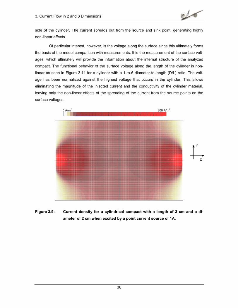
Given a measurement setup with a current source driving the current through the cylin-
drical sample, the above derivation (3.28) in conjunction with (3.17) enables us to calculate and
plot the magnitude of the total current density and the associated relative voltage distribution
throughout the axis-symmetric interior of the compact, as shown in Figure 3.9 and Figure 3.10
respectively. The current injection is accomplished through a single point electrode applied nor-
mal to the surface and acting along the center of the cylinder on either face of the cylinder.
Clearly observable in both figures is the non-uniform field behavior, exhibiting a source region of
maximum strength at the left hand side, and a sink region of minimum strength at the right hand
3. Current Flow in 2 and 3 Dimensions
36
side of the cylinder. The current spreads out from the source and sink point, generating highly
non-linear effects.
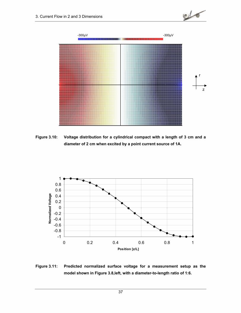
Of particular interest, however, is the voltage along the surface since this ultimately forms
the basis of the model comparison with measurements. It is the measurement of the surface volt-
ages, which ultimately will provide the information about the internal structure of the analyzed
compact. The functional behavior of the surface voltage along the length of the cylinder is non-
linear as seen in Figure 3.11 for a cylinder with a 1-to-6 diameter-to-length (D/L) ratio. The volt-
age has been normalized against the highest voltage that occurs in the cylinder. This allows
eliminating the magnitude of the injected current and the conductivity of the cylinder material,
leaving only the non-linear effects of the spreading of the current from the source points on the
surface voltages.
Figure 3.9: Current density for a cylindrical compact with a length of 3 cm and a di-ameter of 2 cm when excited by a point current source of 1A.
0 A/m2 300 A/m2
r
z
3. Current Flow in 2 and 3 Dimensions
37
Figure 3.10: Voltage distribution for a cylindrical compact with a length of 3 cm and a diameter of 2 cm when excited by a point current source of 1A.
-1-0.8-0.6-0.4-0.2
00.20.40.60.8
1
0 0.2 0.4 0.6 0.8 1Position [z/L]
Nor
mal
ized
Vol
tage
Figure 3.11: Predicted normalized surface voltage for a measurement setup as the model shown in Figure 3.8,left, with a diameter-to-length ratio of 1:6.
r
z
-300µV -300µV
3. Current Flow in 2 and 3 Dimensions
38
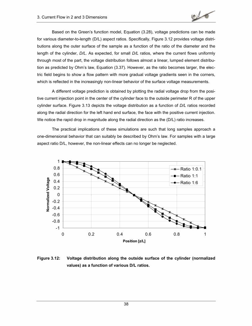
Based on the Green’s function model, Equation (3.28), voltage predictions can be made
for various diameter-to-length (D/L) aspect ratios. Specifically, Figure 3.12 provides voltage distri-
butions along the outer surface of the sample as a function of the ratio of the diameter and the
length of the cylinder, D/L. As expected, for small D/L ratios, where the current flows uniformly
through most of the part, the voltage distribution follows almost a linear, lumped element distribu-
tion as predicted by Ohm’s law, Equation (3.37). However, as the ratio becomes larger, the elec-
tric field begins to show a flow pattern with more gradual voltage gradients seen in the corners,
which is reflected in the increasingly non-linear behavior of the surface voltage measurements.
A different voltage prediction is obtained by plotting the radial voltage drop from the posi-
tive current injection point in the center of the cylinder face to the outside perimeter R of the upper
cylinder surface. Figure 3.13 depicts the voltage distribution as a function of D/L ratios recorded
along the radial direction for the left hand end surface, the face with the positive current injection.
We notice the rapid drop in magnitude along the radial direction as the (D/L) ratio increases.
The practical implications of these simulations are such that long samples approach a
one-dimensional behavior that can suitably be described by Ohm’s law. For samples with a large
aspect ratio D/L, however, the non-linear effects can no longer be neglected.
-1-0.8-0.6-0.4-0.2
00.20.40.60.8
1
0 0.2 0.4 0.6 0.8 1Position [z/L]
Nor
mal
ized
Vol
tage
Ratio 1:0.1Ratio 1:1Ratio 1:6
Figure 3.12: Voltage distribution along the outside surface of the cylinder (normalized values) as a function of various D/L ratios.
3. Current Flow in 2 and 3 Dimensions
39
-160
-140-120
-100
-80
-60-40
-20
00 0.2 0.4 0.6 0.8 1
Position [r/R]
Volta
ge D
rop
[dB
] Ratio 1:0.5Ratio 1:1Ratio 1:2Ratio1:4Ratio 1:6Ratio 1:8
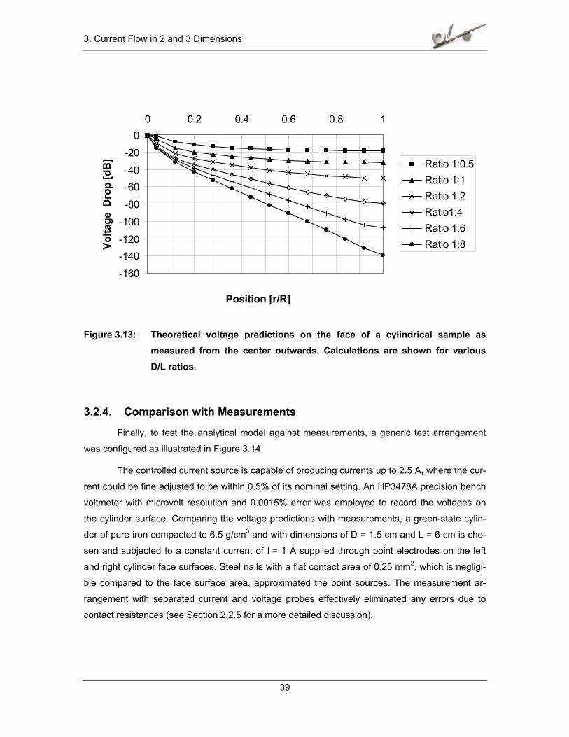
Figure 3.13: Theoretical voltage predictions on the face of a cylindrical sample as measured from the center outwards. Calculations are shown for various D/L ratios.
3.2.4. Comparison with Measurements
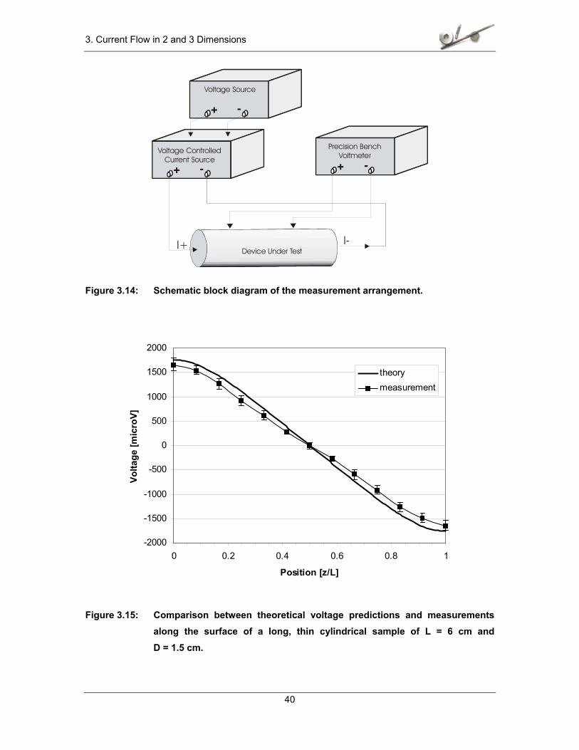
Finally, to test the analytical model against measurements, a generic test arrangement
was configured as illustrated in Figure 3.14.
The controlled current source is capable of producing currents up to 2.5 A, where the cur-
rent could be fine adjusted to be within 0.5% of its nominal setting. An HP3478A precision bench
voltmeter with microvolt resolution and 0.0015% error was employed to record the voltages on
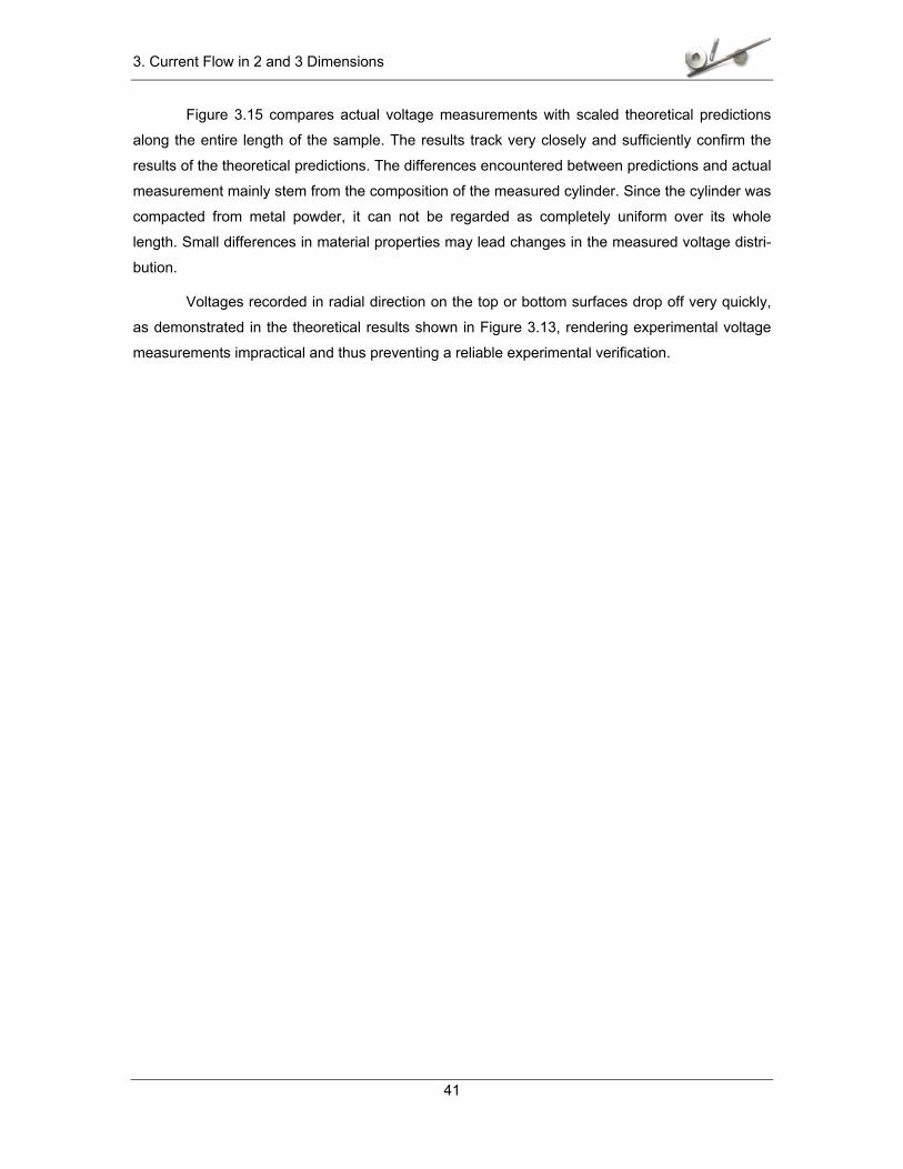
the cylinder surface. Comparing the voltage predictions with measurements, a green-state cylin-
der of pure iron compacted to 6.5 g/cm3 and with dimensions of D = 1.5 cm and L = 6 cm is cho-
sen and subjected to a constant current of I = 1 A supplied through point electrodes on the left
and right cylinder face surfaces. Steel nails with a flat contact area of 0.25 mm2, which is negligi-
ble compared to the face surface area, approximated the point sources. The measurement ar-
rangement with separated current and voltage probes effectively eliminated any errors due to
contact resistances (see Section 2.2.5 for a more detailed discussion).
3. Current Flow in 2 and 3 Dimensions
40
Device Under Test
Voltage ControlledCurrent Source
+ - + -
Precision Bench Voltmeter
+ -
Voltage Source
I+ I-
Figure 3.14: Schematic block diagram of the measurement arrangement.
-2000
-1500
-1000
-500
0
500
1000
1500
2000
0 0.2 0.4 0.6 0.8 1
Position [z/L]
Volta
ge [m
icro
V]
theorymeasurement
Figure 3.15: Comparison between theoretical voltage predictions and measurements along the surface of a long, thin cylindrical sample of L = 6 cm and D = 1.5 cm.
3. Current Flow in 2 and 3 Dimensions
41
Figure 3.15 compares actual voltage measurements with scaled theoretical predictions
along the entire length of the sample. The results track very closely and sufficiently confirm the
results of the theoretical predictions. The differences encountered between predictions and actual
measurement mainly stem from the composition of the measured cylinder. Since the cylinder was
compacted from metal powder, it can not be regarded as completely uniform over its whole
length. Small differences in material properties may lead changes in the measured voltage distri-
bution.
Voltages recorded in radial direction on the top or bottom surfaces drop off very quickly,
as demonstrated in the theoretical results shown in Figure 3.13, rendering experimental voltage
measurements impractical and thus preventing a reliable experimental verification.
4. Conductivity-Density Relationship
42
4 Conductivity-Density Relationship
The conductivity-density relationship for green-state P/M parts lies at the core of our pro-
posed approach to measure density distribution in such compacts. Since we are actually measur-
ing conductivity variations and establishing a conductivity profile of the part, we need to be able to
relate the measured conductivities to a green-state density.
Intuitively we expect the compaction density of a part consisting of metal powders to be
related to its conductivity. Since the literature does not reveal any prior research in this area, the
first step in our approach to detect density variations through conductivity measurements was to
establish this conductivity-density relationship. A series of measurements was conducted and
followed up by theoretical considerations. The following section provides the results of these in-
vestigations.
4.1. Measurements on Green P/M Samples
4.1.1. Measured Parts
Controlled cylindrical green state compacts have been manufactured specifically for the
purpose of conductivity measurements. The cylindrical shape with a large diameter to length ratio
of 4:1 (diameter D = 6cm, length L = 1.5 cm) was chosen for several reasons:
1. The simple cylindrical geometry allows mathematical modeling, and permits a
simple measurement setup.
2. The disc like shape with its short compacted length would assure a uniform den-
sity distribution within the green-state compacts.
3. The large diameter/length ratio would force the current to flow through the inside
of the part rather than on the surface only.
4. Conductivity-Density Relationship
43
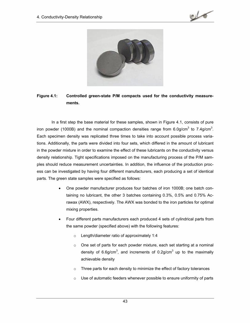
Figure 4.1: Controlled green-state P/M compacts used for the conductivity measure-ments.
In a first step the base material for these samples, shown in Figure 4.1, consists of pure
iron powder (1000B) and the nominal compaction densities range from 6.0g/cm3 to 7.4g/cm3.
Each specimen density was replicated three times to take into account possible process varia-
tions. Additionally, the parts were divided into four sets, which differed in the amount of lubricant
in the powder mixture in order to examine the effect of these lubricants on the conductivity versus
density relationship. Tight specifications imposed on the manufacturing process of the P/M sam-
ples should reduce measurement uncertainties. In addition, the influence of the production proc-
ess can be investigated by having four different manufacturers, each producing a set of identical
parts. The green state samples were specified as follows:
• One powder manufacturer produces four batches of iron 1000B; one batch con-
taining no lubricant, the other 3 batches containing 0.3%, 0.5% and 0.75% Ac-
rawax (AWX), respectively. The AWX was bonded to the iron particles for optimal
mixing properties.
• Four different parts manufacturers each produced 4 sets of cylindrical parts from
the same powder (specified above) with the following features:
o Length/diameter ratio of approximately 1:4
o One set of parts for each powder mixture, each set starting at a nominal
density of 6.6g/cm3, and increments of 0.2g/cm3 up to the maximally
achievable density
o Three parts for each density to minimize the effect of factory tolerances
o Use of automatic feeders whenever possible to ensure uniformity of parts
4. Conductivity-Density Relationship
44
• Additionally, a fifth manufacturer produced parts starting at 6.0g/cm3 in order to
quantify conductivity effects at the lower density scale.
The prepared samples should provide a high degree of reproducibility. Moreover, the
bonding of the AWX to the iron particles should prevent lumps of lubricants within the parts,
thereby minimizing inhomogeneities. The large amount of samples (approximately 280 parts),
prepared by 5 different manufacturers in 5 different production environments and on different ma-
chinery should yield sufficient data to draw conclusions on the conductivity versus density rela-
tionship on a sound basis. Such an approach will assist us to ascertain the dependency of electric
properties on manufacturing influences.
After evaluating the results and establishing a relationship for the above mentioned pow-
der mixtures, the effects of other constituents was to be investigated. The detailed study of the
1000B iron with AWX lubricant raised questions about the qualitative effects of additional alloying
or lubricating constituents in the powder mixture. Although we would not be able to test all possi-
ble combinations of base materials and lubricants, the decision was made to extend the investi-
gations to some additional mixtures. These mixtures were chosen with the goal to answer as
many questions as possible without increasing the number of experiments into unmanageable
proportions. The green-state compacts for these additional tests were made from the following
mixtures:
• 1000B iron powder with zinc stereate (ZnSt) lubricant, to test the effect of a lubri-
cant with larger particle size.
• A series of mixtures from 1000B iron with 0.5% AWX and varying graphite con-
tent to test the influence of different amounts of a conductive lubricant. Six sets of
parts were pressed with the graphite content varying from 0% to 0.8% in 0.2%
increments.
• A complex alloy made from FN-0405 (Ancorsteel 1000B + 3.5% Ni + 0.6% graph-
ite + 0.75% P-11 lubricant + ANCORBOND) which shed light on the effects oc-
curring in parts manufactured from complex mixtures. This powder mixture is
used regularly for industry production.
4.1.2. Setup
The large number of samples required a rather sophisticated measurement setup. How-
ever, the basic measurement concept was very simple: a uniform direct current is injected into the
part through a contact covering the entire surface as shown in Figure 4.2. The resulting homoge-
4. Conductivity-Density Relationship
45
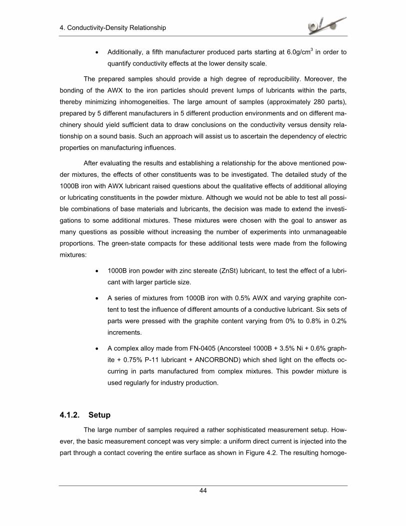
neous current flow produces a surface voltage difference V, which can be directly related to the
conductivity σ of the part through the equation
ALIVσ
= (4.1)
where L represents the length over which the voltage is measured, I is the current strength, and A
represents the surface area of the part.
σ
VV
I I
Aluminum rod
L
Figure 4.2: Current excitation and voltage measurement for controlled green-state samples. The compacts receive the current excitation blocks of aluminum rods covering the entire surface of the sample.
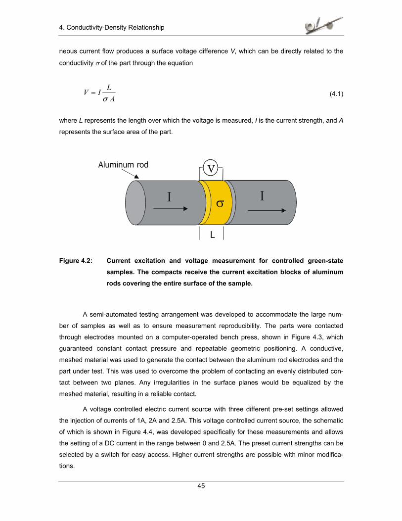
A semi-automated testing arrangement was developed to accommodate the large num-
ber of samples as well as to ensure measurement reproducibility. The parts were contacted
through electrodes mounted on a computer-operated bench press, shown in Figure 4.3, which
guaranteed constant contact pressure and repeatable geometric positioning. A conductive,
meshed material was used to generate the contact between the aluminum rod electrodes and the
part under test. This was used to overcome the problem of contacting an evenly distributed con-
tact between two planes. Any irregularities in the surface planes would be equalized by the
meshed material, resulting in a reliable contact.
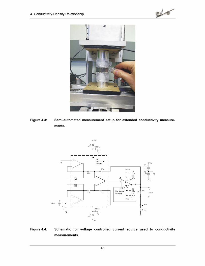
A voltage controlled electric current source with three different pre-set settings allowed
the injection of currents of 1A, 2A and 2.5A. This voltage controlled current source, the schematic
of which is shown in Figure 4.4, was developed specifically for these measurements and allows
the setting of a DC current in the range between 0 and 2.5A. The preset current strengths can be
selected by a switch for easy access. Higher current strengths are possible with minor modifica-
tions.
4. Conductivity-Density Relationship
46
Figure 4.3: Semi-automated measurement setup for extended conductivity measure-ments.
Figure 4.4: Schematic for voltage controlled current source used to conductivity measurements.
4. Conductivity-Density Relationship
47
4.1.3. Sensors
The voltage sensing is, in theory, straightforward. A simple two pin sensor with a fixed
distance between the measuring points will record an identical voltage, wherever it is placed on
the circumference of the green-state compact, as long as it stays aligned with the direction of the
current flow. Such a sensor is depicted in Figure 4.5. Furthermore, this simple configuration pro-
vides a four probe measurement setup with the advantage of the removal of the probe contact
resistances from the measurement results, as discussed previously in section 2.2.5. And since
the current density throughout the volume as well as the conductivity of the sample is assumed
uniform, the voltage drop over a certain length is expected to be constant too without any de-
pendence on the positioning of the sensor.
V
Figure 4.5: Regular two-pin voltage sensor with fixed contact distance.
However, during the measurements it was discovered that changing the position of the two
pin sensor could change the measurement result considerably. The reasons for this phenomenon
are not quite clear, although several possible causes come to mind. First, it is possible that the
mixing process did not produce a completely balanced mixture, so that some areas in the part
receive a higher percentage of lubricant than others. Also lubricant particles could clot together,
again forming regions of higher lubricant concentration. A second possibility is the migration of
lubricant particles toward the part surface during the compaction process. It is well known that
some lubricant migration occurs and that could again lead to an uneven distribution of the non-
conducting lubricant particles. A third possibility is the influence of differences in the surface itself.
The green-state P/M parts have a shiny, smooth surface that looks like solid metal. Inside the
compacts clearly exhibit the grainy structure of pressed powder. These structural differences be-
tween the immediate surface area and the bulk material may influence the conductivity. All these
reasons would lead to a non-uniform conductivity distribution and as a result, make the voltage
measurement dependent on the exact positioning of the two-pin sensor.
In order to overcome the limitations of the two-pin senor, additional sensor configurations
and their applicability have been explored. These sensors were specifically developed to investi-
gate the effects of surface conductivity, geometrical averaging or lubricant migration. One sensor
4. Conductivity-Density Relationship
48
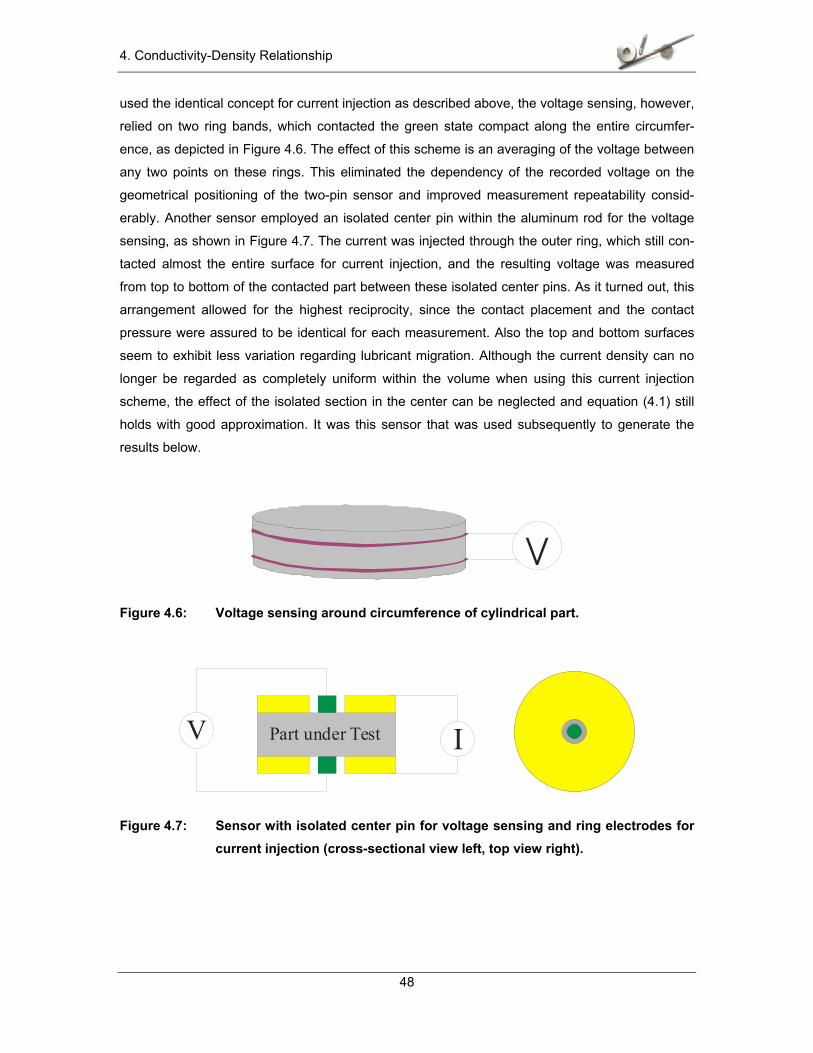
used the identical concept for current injection as described above, the voltage sensing, however,
relied on two ring bands, which contacted the green state compact along the entire circumfer-
ence, as depicted in Figure 4.6. The effect of this scheme is an averaging of the voltage between
any two points on these rings. This eliminated the dependency of the recorded voltage on the
geometrical positioning of the two-pin sensor and improved measurement repeatability consid-
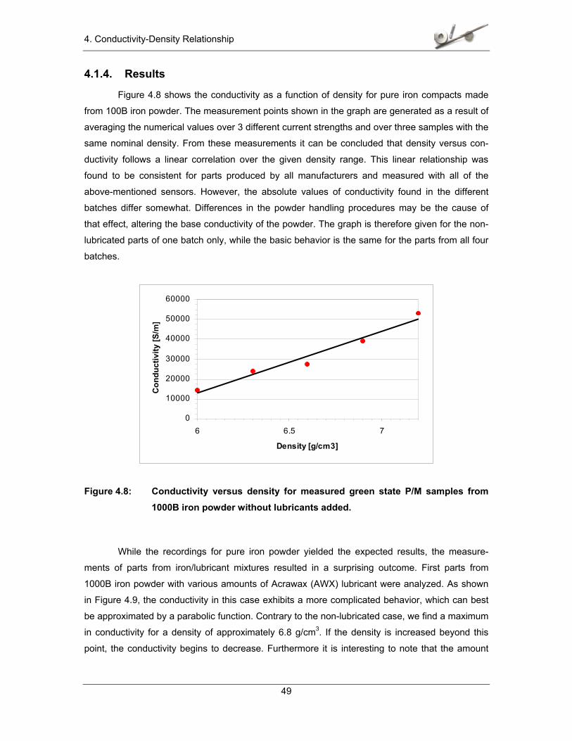
erably. Another sensor employed an isolated center pin within the aluminum rod for the voltage
sensing, as shown in Figure 4.7. The current was injected through the outer ring, which still con-
tacted almost the entire surface for current injection, and the resulting voltage was measured
from top to bottom of the contacted part between these isolated center pins. As it turned out, this
arrangement allowed for the highest reciprocity, since the contact placement and the contact
pressure were assured to be identical for each measurement. Also the top and bottom surfaces
seem to exhibit less variation regarding lubricant migration. Although the current density can no
longer be regarded as completely uniform within the volume when using this current injection
scheme, the effect of the isolated section in the center can be neglected and equation (4.1) still
holds with good approximation. It was this sensor that was used subsequently to generate the
results below.
V
Figure 4.6: Voltage sensing around circumference of cylindrical part.
IV Part under Test
Figure 4.7: Sensor with isolated center pin for voltage sensing and ring electrodes for current injection (cross-sectional view left, top view right).
4. Conductivity-Density Relationship
49
4.1.4. Results
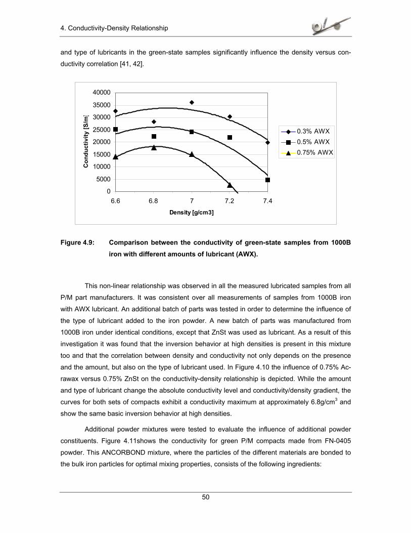
Figure 4.8 shows the conductivity as a function of density for pure iron compacts made
from 100B iron powder. The measurement points shown in the graph are generated as a result of
averaging the numerical values over 3 different current strengths and over three samples with the
same nominal density. From these measurements it can be concluded that density versus con-
ductivity follows a linear correlation over the given density range. This linear relationship was
found to be consistent for parts produced by all manufacturers and measured with all of the
above-mentioned sensors. However, the absolute values of conductivity found in the different
batches differ somewhat. Differences in the powder handling procedures may be the cause of
that effect, altering the base conductivity of the powder. The graph is therefore given for the non-
lubricated parts of one batch only, while the basic behavior is the same for the parts from all four
batches.
0
10000
20000
30000
40000
50000
60000
6 6.5 7
Density [g/cm3]
Con
duct
ivity
[S/m
]
Figure 4.8: Conductivity versus density for measured green state P/M samples from 1000B iron powder without lubricants added.
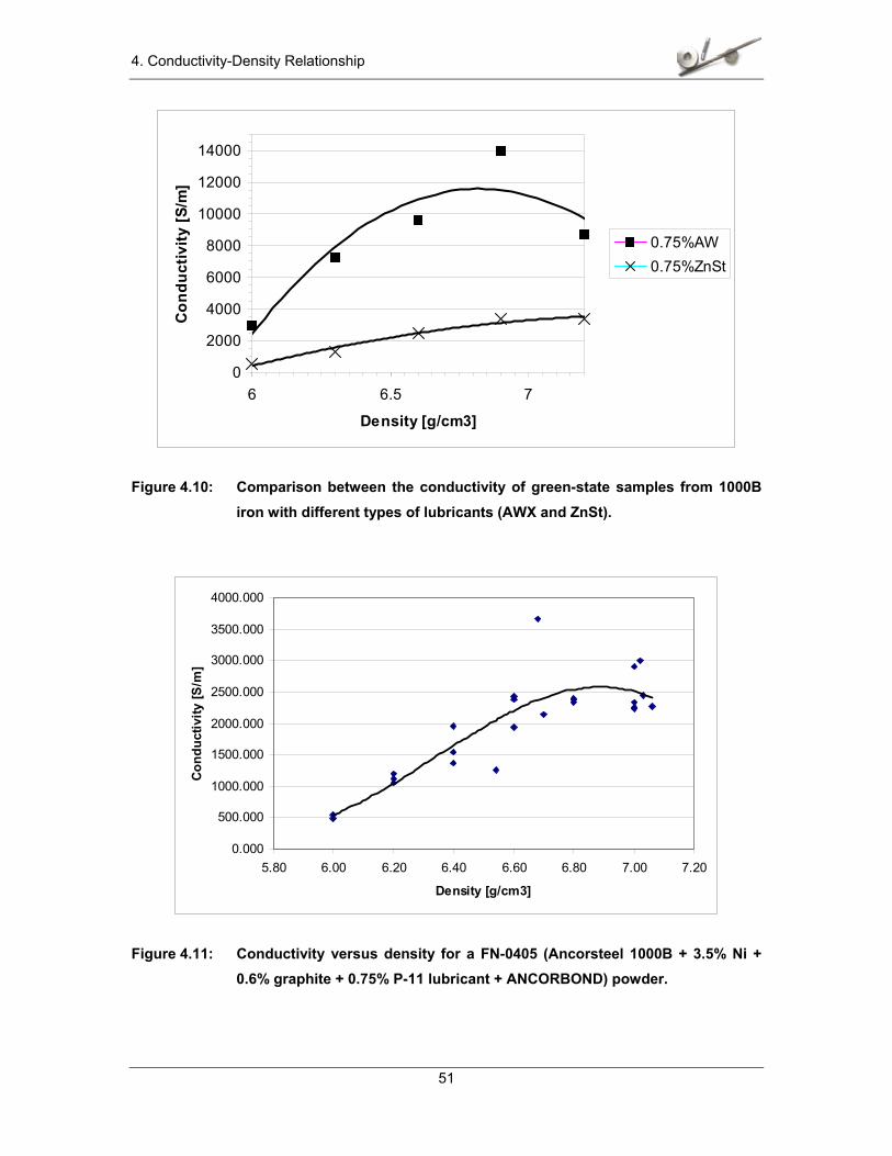
While the recordings for pure iron powder yielded the expected results, the measure-
ments of parts from iron/lubricant mixtures resulted in a surprising outcome. First parts from
1000B iron powder with various amounts of Acrawax (AWX) lubricant were analyzed. As shown
in Figure 4.9, the conductivity in this case exhibits a more complicated behavior, which can best
be approximated by a parabolic function. Contrary to the non-lubricated case, we find a maximum
in conductivity for a density of approximately 6.8 g/cm3. If the density is increased beyond this
point, the conductivity begins to decrease. Furthermore it is interesting to note that the amount
4. Conductivity-Density Relationship
50
and type of lubricants in the green-state samples significantly influence the density versus con-
ductivity correlation [41, 42].
0
5000
10000
15000
20000
25000
30000
35000
40000
6.6 6.8 7 7.2 7.4
Density [g/cm3]
Con
duct
ivity
[S/m
]
0.3% AWX0.5% AWX0.75% AWX
Figure 4.9: Comparison between the conductivity of green-state samples from 1000B iron with different amounts of lubricant (AWX).
This non-linear relationship was observed in all the measured lubricated samples from all
P/M part manufacturers. It was consistent over all measurements of samples from 1000B iron
with AWX lubricant. An additional batch of parts was tested in order to determine the influence of
the type of lubricant added to the iron powder. A new batch of parts was manufactured from
1000B iron under identical conditions, except that ZnSt was used as lubricant. As a result of this
investigation it was found that the inversion behavior at high densities is present in this mixture
too and that the correlation between density and conductivity not only depends on the presence
and the amount, but also on the type of lubricant used. In Figure 4.10 the influence of 0.75% Ac-
rawax versus 0.75% ZnSt on the conductivity-density relationship is depicted. While the amount
and type of lubricant change the absolute conductivity level and conductivity/density gradient, the
curves for both sets of compacts exhibit a conductivity maximum at approximately 6.8g/cm3 and
show the same basic inversion behavior at high densities.
Additional powder mixtures were tested to evaluate the influence of additional powder
constituents. Figure 4.11shows the conductivity for green P/M compacts made from FN-0405
powder. This ANCORBOND mixture, where the particles of the different materials are bonded to
the bulk iron particles for optimal mixing properties, consists of the following ingredients:
4. Conductivity-Density Relationship
51
0
2000
4000
6000
8000
10000
12000
14000
6 6.5 7
Density [g/cm3]
Con
duct
ivity
[S/m
]
0.75%AW0.75%ZnSt
Figure 4.10: Comparison between the conductivity of green-state samples from 1000B iron with different types of lubricants (AWX and ZnSt).
0.000
500.000
1000.000
1500.000
2000.000
2500.000
3000.000
3500.000
4000.000
5.80 6.00 6.20 6.40 6.60 6.80 7.00 7.20
Density [g/cm3]
Cond
uctiv
ity [S
/m]
Figure 4.11: Conductivity versus density for a FN-0405 (Ancorsteel 1000B + 3.5% Ni + 0.6% graphite + 0.75% P-11 lubricant + ANCORBOND) powder.
4. Conductivity-Density Relationship
52
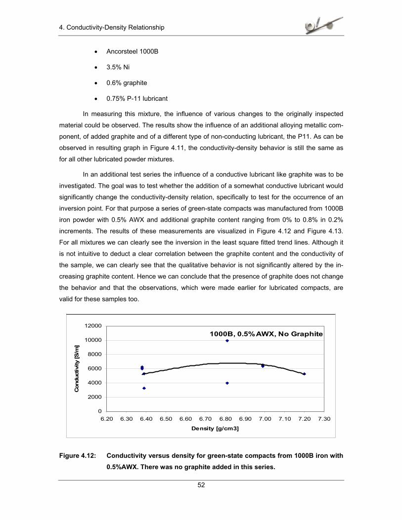
• Ancorsteel 1000B
• 3.5% Ni
• 0.6% graphite
• 0.75% P-11 lubricant
In measuring this mixture, the influence of various changes to the originally inspected
material could be observed. The results show the influence of an additional alloying metallic com-
ponent, of added graphite and of a different type of non-conducting lubricant, the P11. As can be
observed in resulting graph in Figure 4.11, the conductivity-density behavior is still the same as
for all other lubricated powder mixtures.
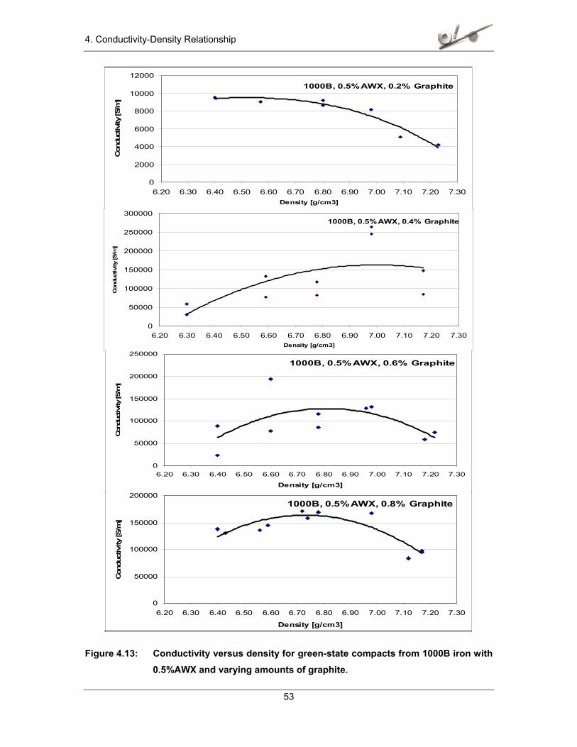
In an additional test series the influence of a conductive lubricant like graphite was to be
investigated. The goal was to test whether the addition of a somewhat conductive lubricant would
significantly change the conductivity-density relation, specifically to test for the occurrence of an
inversion point. For that purpose a series of green-state compacts was manufactured from 1000B
iron powder with 0.5% AWX and additional graphite content ranging from 0% to 0.8% in 0.2%
increments. The results of these measurements are visualized in Figure 4.12 and Figure 4.13.
For all mixtures we can clearly see the inversion in the least square fitted trend lines. Although it
is not intuitive to deduct a clear correlation between the graphite content and the conductivity of
the sample, we can clearly see that the qualitative behavior is not significantly altered by the in-
creasing graphite content. Hence we can conclude that the presence of graphite does not change
the behavior and that the observations, which were made earlier for lubricated compacts, are
Figure 4.13: Conductivity versus density for green-state compacts from 1000B iron with 0.5%AWX and varying amounts of graphite.
4. Conductivity-Density Relationship
54
4.2. Conductivity of Mixtures
4.2.1. Non-Conducting Particles in Conducting Medium
There are many reasons why the apparent averaged conductivity in P/M components
containing lubricants may decrease with increasing density (as seen for example in Figure 4.9).
Some of these are:
• Lamination effects
• Lubricant migration
• Increased corrosion
However, none of the above does sufficiently explain the observed results.
The one phenomenon in lubricant containing P/M compacts that has the potential to
cause a non-linear relationship is the redistribution and geometrical deformation of the lubricant
upon compaction, thus affecting the electrostatic response of the compact. This phenomenon and
its underlying theory are further elaborated below.
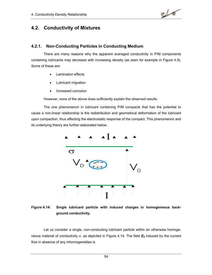
+++---
V0VD
σ
Figure 4.14: Single lubricant particle with induced charges in homogeneous back-ground conductivity.
Let us consider a single, non-conducting lubricant particle within an otherwise homoge-
neous material of conductivity σ, as depicted in Figure 4.14. The field E0 induced by the current
flow in absence of any inhomogeneities is
4. Conductivity-Density Relationship
55
001 JEσ
= . (4.2)
The non-conducting lubricant particle can be regarded as a depolarizing dipole, whose
field is generated by surface charges induced by the impressed current density J. The surface
charges on the non-conducting particle orient themselves in such a way that they annihilate the
local field at the particle boundaries. As a result, the depolarization field is oriented in the same
way as the global field E0.This dipole field contributes to the voltage measured at the outside of
the part so that the outside voltage becomes
DVVV += 0 . (4.3)
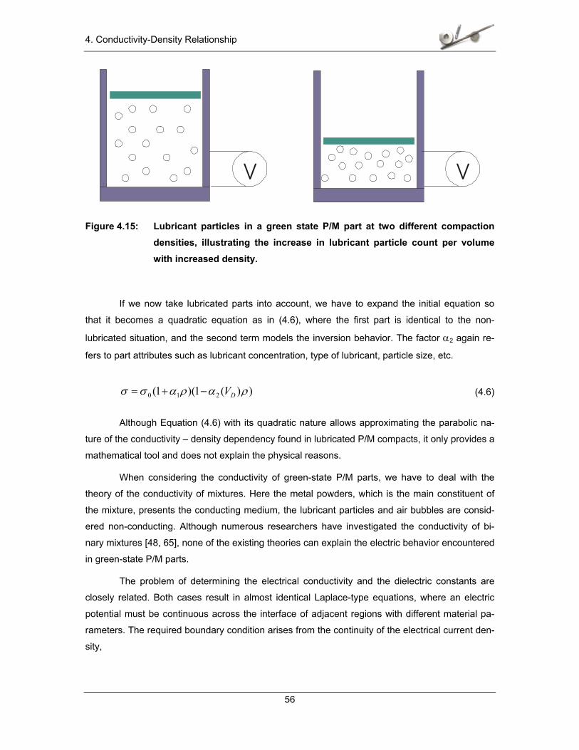
If we next contemplate the situation as depicted in Figure 4.15, where a powder/lubricant
mixture is shown at two different compaction states, we deduce an increase of lubricant particles
within a given volume at high densities. Since each of these particles generates a dipole field, we
have to conclude that the total induced voltage VD, which is the sum of the dipole voltages over
all lubricant particles, increases at the circumference of the part. Keeping the impressed current I
constant, this results in an increase of the measured resistance as seen in (4.4):
AL
IVV
IVR D
σ=
+== 0 (4.4)
where V0 is the voltage due to the background conductivity σ0 and VD is the sum of the dipole
potentials.
These results allow us to model the conductivity-density relationship of a non-lubricated
part by a linear equation as given in (4.5)
)1( 10 ρασσ += , (4.5)
where σ0 refers to the background conductivity and α1 is a constant model parameter.
4. Conductivity-Density Relationship
56
V V
Figure 4.15: Lubricant particles in a green state P/M part at two different compaction densities, illustrating the increase in lubricant particle count per volume with increased density.
If we now take lubricated parts into account, we have to expand the initial equation so
that it becomes a quadratic equation as in (4.6), where the first part is identical to the non-
lubricated situation, and the second term models the inversion behavior. The factor α2 again re-
fers to part attributes such as lubricant concentration, type of lubricant, particle size, etc.
))(1)(1( 210 ραρασσ DV−+= (4.6)
Although Equation (4.6) with its quadratic nature allows approximating the parabolic na-
ture of the conductivity – density dependency found in lubricated P/M compacts, it only provides a
mathematical tool and does not explain the physical reasons.
When considering the conductivity of green-state P/M parts, we have to deal with the
theory of the conductivity of mixtures. Here the metal powders, which is the main constituent of
the mixture, presents the conducting medium, the lubricant particles and air bubbles are consid-
ered non-conducting. Although numerous researchers have investigated the conductivity of bi-
nary mixtures [48, 65], none of the existing theories can explain the electric behavior encountered
in green-state P/M parts.
The problem of determining the electrical conductivity and the dielectric constants are
closely related. Both cases result in almost identical Laplace-type equations, where an electric
potential must be continuous across the interface of adjacent regions with different material pa-
rameters. The required boundary condition arises from the continuity of the electrical current den-
sity,
4. Conductivity-Density Relationship
57
EJ σ= , (4.7)
perpendicular to the interface in the conductive case. Here σ denotes the electric conductivity and
Ε is the electric field. Furthermore, the continuity of the displacement,
ED ε= (4.8)
perpendicular to the interface must be maintained (ε represents the dielectric constant). Since the
field E plays the same role in both cases, the governing equations for the conductivity and the
dielectric constant become identical.
If the non-conducting particles in a conducting medium are treated like molecules in a
solid or liquid dielectric spaced in such a way that we can assume that the effect of their presence
does not considerably alter the electric field acting on the neighboring particles, then the Clau-
sius-Mossotti equation applies:
effeff nLEPEE3
43
400
πεπεε ==− (4.9)
This equation calculates the summed effect of all particles within the volume due to the
external electric field E0, resulting in an effective field Eeff. Here P is the macroscopic polarization
vector, n is the particle concentration, and L represents the depolarization factor. Such a model
appears to be a plausible explanation, as the lubricant can be considered as individual particles
embedded in the green-state P/M base material. Since the lubricant concentration is generally
low, on the order of 5% or less, the mutual interaction between the polarizable particles can be
neglected. The sum of their effects, however, still leads to an effective field that differs from the
applied field.
The idea of having two separate material constituents with different electric properties
can also be treated from a purely mechanical point of view. Considering a medium consisting of
two (or more) constituents with conductivities 1σ and 2σ and volume fractions 1f and 2f on a
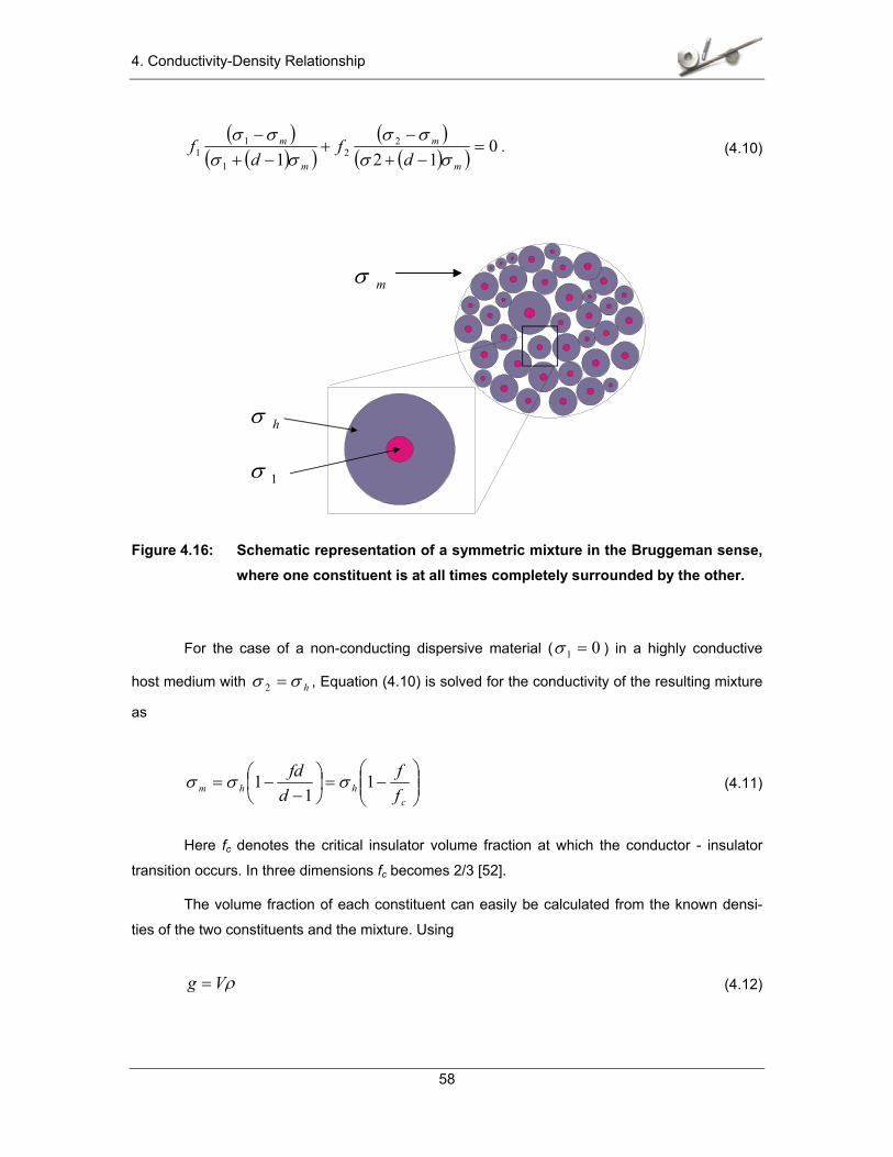
completely symmetrical basis, leads to Bruggeman’s symmetric theory [11, 21]. This theory al-
lows us to calculate the conductivity of a random mixture of spherical particles of two constitu-
ents, both of which completely fill the medium as depicted in Figure 4.16. Generalizing the equa-
tion to three dimensions d=1,2,3, the conductivity of medium mσ is thus given by the equation
[51, 54]
4. Conductivity-Density Relationship
58
( )( )( )
( )( )( ) 0
1212
21
11 =
−+−
+−+
−
m
m
m
m
df
df
σσσσ
σσσσ
. (4.10)
mσ
hσ
1σ
Figure 4.16: Schematic representation of a symmetric mixture in the Bruggeman sense, where one constituent is at all times completely surrounded by the other.
For the case of a non-conducting dispersive material ( 01 =σ ) in a highly conductive
host medium with hσσ =2 , Equation (4.10) is solved for the conductivity of the resulting mixture
as
−=
−−=
chhm f
fdfd 1
11 σσσ (4.11)
Here fc denotes the critical insulator volume fraction at which the conductor - insulator
transition occurs. In three dimensions fc becomes 2/3 [52].
The volume fraction of each constituent can easily be calculated from the known densi-
ties of the two constituents and the mixture. Using
ρVg = (4.12)
4. Conductivity-Density Relationship
59
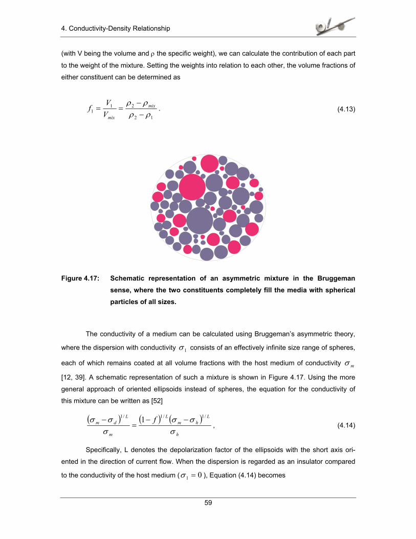
(with V being the volume and ρ the specific weight), we can calculate the contribution of each part
to the weight of the mixture. Setting the weights into relation to each other, the volume fractions of
either constituent can be determined as
12
211 ρρ
ρρ−−
== mix
mixVV
f . (4.13)
Figure 4.17: Schematic representation of an asymmetric mixture in the Bruggeman sense, where the two constituents completely fill the media with spherical particles of all sizes.
The conductivity of a medium can be calculated using Bruggeman’s asymmetric theory,
where the dispersion with conductivity 1σ consists of an effectively infinite size range of spheres,
each of which remains coated at all volume fractions with the host medium of conductivity mσ
[12, 39]. A schematic representation of such a mixture is shown in Figure 4.17. Using the more
general approach of oriented ellipsoids instead of spheres, the equation for the conductivity of
this mixture can be written as [52]
( ) ( ) ( )h
Lhm
L
m
Ldm f
σσσ
σσσ /1/1/1 1 −−
=−
, (4.14)
Specifically, L denotes the depolarization factor of the ellipsoids with the short axis ori-
ented in the direction of current flow. When the dispersion is regarded as an insulator compared
to the conductivity of the host medium ( 01 =σ ), Equation (4.14) becomes
4. Conductivity-Density Relationship
60
( ) Lhm f −−= 11
1σσ . (4.15)
Combining the two theories into a semi-phenomenological effective medium equation de-
veloped by McLachlan [53] results in one equation that allows us to treat media whose morpholo-
gies are those of the symmetric and asymmetric media of Bruggeman or lie in between these two
extremes. The generalized effective medium equation is therefore given by
( ) ( ) ( )0
1
1
1/1/1
2
/1/12
/1/11
/1/11 =
−+
−−+
−+
−t
mc
ct
tm
tc
tm
c
ct
tm
t
ff
f
ff
f
σσ
σσ
σσ
σσ.
(4.16)
with )1/( Lft c −= for oriented ellipsoids and fc being the volume fraction at which the conductor-
insulator transition occurs. Again assuming 01 =σ , we find
t
chm f
f
−= 1σσ (4.17)
for the conductivity of the mixture. Although this equation can be used for any mixture and mor-
phology type, the value for fc is not readily available. Furthermore we can assume that in our case
all the lubricant particles will be surrounded by the metal powder, since the volume fraction of the
lubricant is very low. Hence, we may use Bruggeman’s equation for asymmetric media as given
in (4.15).
Modeling the conductivity of a green state P/M compact was accomplished by calculating
the volume fraction of air and lubricant at each density. Employing Equation (4.15), the conductiv-
ity for non-lubricated parts was calculated with the conductivity iron as the base material. In a
next step, the resulting conductivity was used as the background conductivity in the calculation of
the lubricated parts, resulting in an overall equation of
( ) ( ) lub11
lub11
11 LLairFePM ff air −− −−= σσ . (4.18)
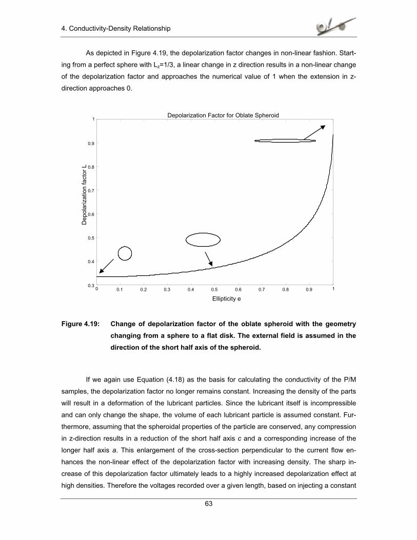
Using these parameters to simulate the conductivity–density relationship over a wide
density range does not show the results we obtained during the experiments. Although the vol-
ume fractions for the air and the lubricant account for a reduction in the overall conductivity, the
functional relationship stays linear. This is explained by the fact that the volume fraction of the
4. Conductivity-Density Relationship
61
lubricant remains constant through the compaction process. The increased amounts of non-
conducting lubricant particles per volume at high densities only result in a lower slope in the still
linear relationship and cannot explain the inversion behavior.
4.2.2. Depolarization Effect
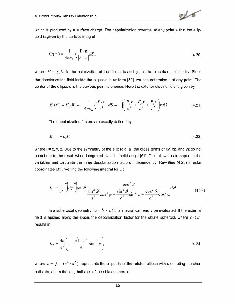
In the previous section the lubricant particles and the air inclusions within the pressed
part are considered as perfect spheres. As seen above, the linear increase of low-conducting par-
ticles per volume with a linear increase in density leads to a linearly increasing conductivity,
where the amount of lubricant in the mixture determines the slope of the relationship. While a
spherical shape is a valid approximation for the lubricant particles in the non-compacted state, the
compaction process deforms the lubricant particles to spheroidal shapes [45]. Unlike the simple
increase of lubricant particles per volume at higher densities as seen in Figure 4.15, we now con-
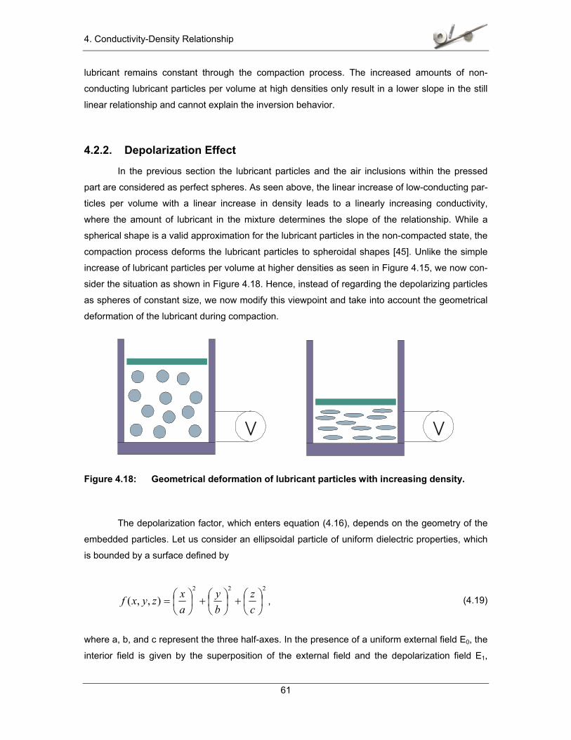
sider the situation as shown in Figure 4.18. Hence, instead of regarding the depolarizing particles
as spheres of constant size, we now modify this viewpoint and take into account the geometrical
deformation of the lubricant during compaction.
V V
Figure 4.18: Geometrical deformation of lubricant particles with increasing density.
The depolarization factor, which enters equation (4.16), depends on the geometry of the
embedded particles. Let us consider an ellipsoidal particle of uniform dielectric properties, which
is bounded by a surface defined by
222
),,(
+
+
=
cz
by
axzyxf , (4.19)
where a, b, and c represent the three half-axes. In the presence of a uniform external field E0, the
interior field is given by the superposition of the external field and the depolarization field E1,
4. Conductivity-Density Relationship
62
which is produced by a surface charge. The depolarization potential at any point within the ellip-
soid is given by the surface integral
dSrr
r ∫ −⋅
=Φ'4
1)'(0
nPπε
, (4.20)
where 1EP eχ= is the polarization of the dielectric and eχ is the electric susceptibility. Since
the depolarization field inside the ellipsoid is uniform [50], we can determine it at any point. The
center of the ellipsoid is the obvious point to choose. Here the exterior electric field is given by
Ω
++−=
⋅−== ∫∫ rd
czP
byP
axP
dSrrnPErE zyx
22230
11 41)0()'(πε
. (4.21)
The depolarization factors are usually defined by
iii PLE −=1 , (4.22)
where i = x, y, z. Due to the symmetry of the ellipsoid, all the cross terms of xy, xz, and yz do not
contribute to the result when integrated over the solid angle [61]. This allows us to separate the
variables and calculate the three depolarization factors independently. Rewriting (4.23) in polar
coordinates [81], we find the following integral for Lz:
ϑϕϑϕϑϕϑ
ϑϑϕπ π
∂++
∂= ∫ ∫2
0
2
0 22
22
2
22
2
2
2
2
coscossinsincossincossin1
cbac
Lz (4.23)
In a spheroidal geometry ( cba ≠= ) this integral can easily be evaluated. If the external
field is applied along the z-axis the depolarization factor for the oblate spheroid, where ac < ,
results in
,sin114 12
2
−−= − e
ee
eLZ
π (4.24)
where )/(1 22 ace −= represents the ellipticity of the rotated ellipse with c denoting the short
half-axis, and a the long half-axis of the oblate spheroid.
4. Conductivity-Density Relationship
63
As depicted in Figure 4.19, the depolarization factor changes in non-linear fashion. Start-
ing from a perfect sphere with Lz=1/3, a linear change in z direction results in a non-linear change
of the depolarization factor and approaches the numerical value of 1 when the extension in z-
direction approaches 0.
0 0.1 0.2 0.3 0.4 0.5 0.6 0.7 0.8 0.9 1 0.3
0.4
0.5
0.6
0.7
0.8
0.9
1 Depolarization Factor for Oblate Spheroid
Ellipticity e
Dep
olar
izat
ion
fact
or L
Figure 4.19: Change of depolarization factor of the oblate spheroid with the geometry changing from a sphere to a flat disk. The external field is assumed in the direction of the short half axis of the spheroid.
If we again use Equation (4.18) as the basis for calculating the conductivity of the P/M
samples, the depolarization factor no longer remains constant. Increasing the density of the parts
will result in a deformation of the lubricant particles. Since the lubricant itself is incompressible
and can only change the shape, the volume of each lubricant particle is assumed constant. Fur-
thermore, assuming that the spheroidal properties of the particle are conserved, any compression
in z-direction results in a reduction of the short half axis c and a corresponding increase of the
longer half axis a. This enlargement of the cross-section perpendicular to the current flow en-
hances the non-linear effect of the depolarization factor with increasing density. The sharp in-
crease of this depolarization factor ultimately leads to a highly increased depolarization effect at
high densities. Therefore the voltages recorded over a given length, based on injecting a constant
4. Conductivity-Density Relationship
64
DC current, begin to increase. This, in turn, leads to the experimentally observed decrease in
conductivity at high densities.
Figure 4.20 demonstrates the simulation of Equation (4.18) over a large range of nominal
densities. We can clearly see the linear behavior for the non-lubricated powder as well as the in-
version behavior for the mixtures containing various amounts of lubricants.
6000 6200 6400 6600 6800 7000 7200 7400 7600 6
6.5
7
7.5
8
8.5
9
9.5
10 x 10 6 Conductivity vs. Density
Density [g/cm3]
Con
duct
ivity
[S/m
] 0.375%AWX
0.5%AWX
0.75%AWX
No Lub
Figure 4.20: Simulation of conductivity vs. density behavior for green state P/M parts with different amount of lubricants.
Although a physical explanation for the qualitative behavior could be found in the above
developed theory of the conductivity of green-state P/M parts, it is clear from a direct comparison
of the absolute values of the simulated graph to the real measurements that there are still differ-
ences. The many parameters that are available to adjust the theory have not yet been further in-
vestigated. Some of the effects that have to be taken into account are:
• Base conductivity of 100% dense iron powder is not the same as of pure iron, as
assumed in the simulation.
4. Conductivity-Density Relationship
65
• Grain size is not currently included in the model but definitively impacts both the
base conductivity through the contact area between grains and the deformation
properties of the mixture.
• Density at which lubricant deformation starts to be effective (after rearranging in
the first part of compaction).
• Rate of lubricant deformation.
These and certainly some additional effects have to be investigated more thoroughly if
one wants to model the conductivity – density behavior more closely. However, since our goal
was to prove the existence of such a relationship and subsequently explain the physical basis, we
did not pursue these contemplations any further. Additional work is required should one want to
generate a universal formula for the calculation of the conductivity of green-state P/M compacts
at all densities.
4.3. Conductivity-Density Relationship for Green P/M Samples The conductivity-density relationship for green-state P/M samples lies at the core of our
proposed approach to the measurement of density variations throughout the volume of a sample
by injecting currents and conducting voltage measurements on its surface. Since we are basically
measuring conductivities, the ability to relate the recorded conductivity to a certain density is a
necessity. The extensive measurements together with the theoretical considerations produced
some interesting results in this respect.
The nature of the conductivity-density relationship for green-state P/M samples is not in-
dependent of the powder mixture. While it was expected that the absolute value of the conductiv-
ity would change with the conductivity of the main powder constituents, the qualitative difference
encountered between lubricated and non-lubricated parts was surprising. It was found that the
relationship for non-lubricated parts follows a linear dependency over the whole density range.
This allows for easy reconstruction of densities from any given conductivity measurement over
the whole range.
The relationship in lubricated parts is more complex and is not only non-linear, but it even
exhibits an inversion from the expected line at high densities, meaning that the conductivity actu-
ally decreases with increasing density after a certain point. This qualitative behavior was found in
all samples made from a mixture containing a non-conducting lubricant. The physical considera-
tions detailed in section 4.2 above explain the occurrence of this phenomenon.
4. Conductivity-Density Relationship
66
The inversion effect renders the density calculation from the measured conductivity more
complicated than in the linear case. Even more important, it places some physical constraints to
the applicability of our method. Since the sensitivity on the conductivity due to density variations
is zero or almost zero in the vicinity of the inversion point, variations around this point cannot be
detected with our method. The approach is therefore ill-suited to analyze compacts whose nomi-
nal density is at or near the inversion point. However, since the industry trend goes to ever in-
creasing densities, most parts manufactured will stay well “to the right” of the inversion point and
will not be affected by this limitation. Also, since this inversion point changes with changing pow-
der mixture, a general statement about the ability to measure parts of a certain density cannot be
made. It has to be determined for each mixture individually.
0
5000
10000
15000
20000
25000
30000
6.6 6.8 7 7.2 7.4Density [g/cm3]
Con
duct
ivity
[S/m
]
Figure 4.21: Two different densities with the same conductivity in a green-state sample of 1000B with 0.5% AWX.
Additionally, the inversion behavior produces an ambiguity for the density reconstruction.
Since the conductivity decreases again with increasing density, there are usually two densities for
any given conductivity reading, as shown in Figure 4.21. Naturally, this would prevent a success-
ful density reconstruction from a conductivity measurement. This complication can be overcome
with the additional information that is usually available when analyzing a compact. When we are
given a green-state sample with a nominal density of 7.1g/cm3, we can expect a reading in the
vicinity of this nominal value. Should a measurement result in a conductivity of 24000S/m, we
could therefore conclude that the density must be 7.02g/cm3. And after we have established a
Different densities,
same conductivity
4. Conductivity-Density Relationship
67
number of density values, we know that the density will vary only gradually. Any new reading
taken in the vicinity of the previous ones will not show a drastically different density value. This
again gives us enough information to overcome the ambiguity and to select the correct density
value when presented with a new conductivity measurement.
Although the nature of the conductivity-density behavior encountered in lubricated green-
state P/M samples somewhat complicates the task of measuring density by recording conductivi-
ties, the proposed method can still be used successfully in most cases.
5. Electric Impedance Tomography
68
5 Electric Impedance Tomography
5.1. Introduction
5.1.1. Definition of Tomography
The term tomography refers to a general procedure for the synthesis of two-dimensional
(2D) cross-sectional images or slices of a three-dimensional (3D) object. The images are ob-
tained from external measurements of a spatially varying function. Line integrals are the most
common external measures, which are also known as projections. Availability of multiple projec-
tions at different orientations allows accurate recovery of the original tomogram. Additionally,
several of these 2D images can be stacked together to obtain a 3D representation of the object.
Tomographic systems allow one to view the internal structure of objects in a noninvasive
and nondestructive manner. There are several methods available to record these 2D images and,
depending on the specific method, tomographic inspection can be used for many different appli-
cations. Because practical implementation of tomography typically requires the management of a
large amount of data combined with extensive numerical calculations, modern computing tech-
nology is indispensable for tomographic applications. Hence, the term CT for computerized tomo-
graphy applies to all of today’s tomographic applications.
By far the best known tomographic application is the X-ray imaging of the human body. A
commercial X-ray imaging system is shown in Figure 5.1. Other medical devices, including ultra-
sonic scanners and magnetic resonance imaging systems, also make use of tomographic princi-
ples. Outside the medical realm, tomography is used in applications ranging from microscopy
through nondestructive material testing and radar imaging to geophysical imaging and radio as-
tronomy.
5. Electric Impedance Tomography
69
Figure 5.1: Medical X-ray CT system, which conducts scanning 2D projections and re-constructs 3D images.
In order to understand the advantages of tomographic image reconstruction, let us look at
the differences between conventional X-ray radiography and X-ray computer tomography. In con-
ventional X-ray radiography, a stationary source and planar detector are used to produce a 2D
projection image of the patient. This image has an intensity proportional to the amount by which
the X rays are attenuated as they pass through the body. In other words, the 3D spatial distribu-
tion of X-ray attenuation coefficients is projected into a 2D image. The resulting image provides
important diagnostic information due to differences in the attenuation coefficients of bone, mus-
cle, fat, and other tissues in the 40 keV to 120 keV range used in clinical radiography. The utility
of conventional radiography is limited by the fact that the 3D anatomy is projected into a 2D im-
age, causing certain structures to be obscured. For example, tumors in the lung may be obscured
by a more dense rib that projects into the same area in the radiograph.
Computerized tomography systems do not form the image directly as in the case of con-
ventional techniques. Instead, several 2D pictures are obtained by rotating the source and detec-
tor around the investigated object. The sampled data are processed by an image-reconstruction
algorithm to produce a digital representation of the desired image. A computed tomography sys-
tem collects measurements of 1D line integrals, or projections, along parallel paths through a 2D
slice of a 3D object. By collecting these projections at different angles relative to a fixed coordi-
nate system, we build up the 2D Radon transform from which the image is reconstructed. This
function is based on the theories around the properties of the integrals of N-D functions over (N -
1)-D hyperplanes.
5. Electric Impedance Tomography
70
In the early days of computing, one major limitation of the first generation of CT systems
was that a single scan would take several minutes and the subsequent computational time again
would be on the order of several minutes for a single image. Using modern scanning techniques
and the computational power of today’s computers, modern scanners can scan a single plane in
less than one second.
Tomographic principles have also been applied in a number of other diagnostic medical
imaging instruments. One major application, for which the early developments actually were re-
searched before X-ray CT, is nuclear imaging. Based on the same principle of measuring the
varying absorption of electromagnetic waves, measurements of physiological processes are ob-
tained by tomographic imaging of the spatial distribution of a biochemical tracer or probe that has
been tagged with a radioactive isotope. Using these systems with various probes, it is possible to
produce 3D images of metabolic activity throughout the body, variations in neurotransmitter and
receptor densities in the brain, and the functioning of the heart and blood vessels.
Magnetic resonance imaging (MRI), another well known tomographic application in the
medical field, differs from X-ray and emission CT in the sense that the image Fourier transform or
“k-space” is measured directly. This is achieved by using a magnetic field gradient to produce a
spatial frequency-encoding of the magnetic resonance signal from hydrogen nuclei in the body.
Using combinations of time-varying magnetic field gradients and radio-frequency pulses, it is pos-
sible to obtain k-space measurements with a wide range of sampling patterns. This encoding al-
lows measuring the response from each sub-volume separately and provides an easy way to
build an image.
Tomographic methods have also proven very powerful in applications other than medical
imaging. Different systems have been widely used for nondestructive testing of manufactured
components and materials. Tomography has also had an enormous impact in exploring the natu-
ral world. Applications range from microscopic imaging using electron micrographs and micro-
scopes to imaging of celestial bodies using radio telescopes. Electromagnetic techniques have
been used for resistivity imaging between bore holes in geophysical applications and imaging of
ionospherical electron density. Similarly, acoustical signals have been used for tomographic im-
aging over a wide range of scales from acoustic microscopy to large-scale mapping of the oceans
grounds, as well as 3D mapping of the earth's interior using natural seismic data.
5.1.2. Principles of Electric Impedance Tomography
Electric Impedance Tomography (EIT) refers to a specific method to acquire the data
used in the tomographic reconstruction. According to its name, it characterizes and images the
distribution of the electric impedances in the analyzed object. EIT is a non-invasive, non-
5. Electric Impedance Tomography
71
destructive technique, in which we inject currents into a body and measure the resulting electric
potential using electrodes placed on the boundary of the volume. Then, using this boundary data
of current and voltage measurements, the internal electric impedance of the inspected volume is
reconstructed and visualized in either a 2D or 3D graph.
EIT provides a technique to inspect the internal electric impedance or conductivity from
external measurements. The knowledge of this conductivity distribution can then be used to de-
termine certain properties of the volume that is to be analyzed without having physical access to
the inner regions of this volume. Of course it is essential that the investigated property is linked to
the electric impedance of the body and that changes in the material result in changes of the im-
pedance. Key properties of the EIT method are:
• Non-destructive, non-invasive access to internal sections of the analyzed vol-
ume.
• Low cost
• Low risk
• Compact system
• Visualization of properties
Like all other tomographic applications, EIT has its limitations. For EIT, these include the
inability to probe enclosed high impedance layers due to the limited current penetration into these
regions, and low resolution, due to the limited number of independent measurements that are
feasible. These limitations dictate the applicability of EIT to certain measurement conditions. In
general, EIT is best suited to measure impedance variations over large distances compared to
the electrode placement, or to monitor impedance changes with time.
Impedance imaging was first developed by Dynes and Lytle in 1981 [65]. Its application
to the medical field, which is today’s best known and most researched application of the method,
was introduced in 1982 by Barber and Brown [6]. Since different tissues in the human body have
different impedances, it is possible to discriminate tissues from the impedance measurements as
well as to detect physiological events that change the electric impedance of the tissue.
Whether the application of EIT is of medical nature or not, the principles of the method
remain largely the same in all cases. A direct or alternating current is injected into the inspected
volume through strategically placed surface electrodes. Differential voltage measurements
through the remaining electrodes are recorded. Usually, the current injection and voltage re-
cording pattern is varied and several measurements with different configurations are taken. The
voltage data from these measurements is then fed to a reconstruction algorithm that calculates
5. Electric Impedance Tomography
72
the impedance distribution in the tested volume. Figure 5.2 shows a block diagram of the main
components of an EIT system.
Figure 5.2: Generic system arrangement of EIT.
Due to the nature of the physical phenomenon employed to discriminate between regions
exhibiting varying properties, the reconstruction of the impedance distribution from the recorded
data is quite complicated. Unlike X-ray CT, where the image represents a line integral of the ab-
sorption characteristics of the material, the voltage distribution resulting from a specific current
injection pattern is very difficult to calculate. Since the electric currents do not follow a predefined,
well known path, but rather are influenced by the unknown impedance distribution of the material,
the task of reconstructing the impedance is much more daunting. The fact that the current flow
and hence, the voltage distribution, is influenced by the unknown medium property, calls for an
iterative procedure to calculate it.
Similar to other tomographic techniques, EIT is used by applying a source of energy, in
this case electric current, to the boundary of the volume of interest. Through a number of elec-
trodes placed on the same boundary, the absorption characteristics of the material to the specific
form of energy are recorded, here in the form of electric potentials. In order to find the distribution
of the unknown physical property, the impedance, we have to solve two separate problems. First,
we need to solve the so called forward problem. Given the boundary conditions of the current in-
jection and flux free boundaries as well as the conductivity distribution, the forward problem cal-
culates the expected voltage distribution throughout the volume. Starting with Laplace’s equation
(3.2), the electric potential in the volume is calculated. Since for most volume shapes it is not
Current source unit
Voltage meas-urement circuit
Control and data acquisition unit
Reconstruction algorithm
5. Electric Impedance Tomography
73
possible to do so in closed form, numerical techniques have to be used instead. Therefore, the
forward problem usually involves the setup of a numerical model based on the model parameters,
and result in a prediction of what the data would look like, if the parameters were as assumed. In
the second step, the actual data is compared to the data prediction obtained from the forward
problem. The differences between the actual and the predicted data lead to a new estimation of
the model parameters through the solution of the so called Inverse Problem.
The inverse problem tries to find the model parameters, given the boundary conditions
and the measurement data. Figure 5.3 illustrates the differences between the forward and the
inverse problem. As suggested by their names, the data flow in the two problems is directly oppo-
site. In the forward case, we assume to know all the model parameters and material properties,
from which we can then calculate the system data at any point. In the inverse problem, on the
other hand, we know the data from measurements and try to calculate the material parameters.
Figure 5.3: Differences between the forward and the inverse problem.
In some cases it is possible to directly solve for the model parameters using an inverse
solution to the forward approach. In these cases, a system of linear equations with model pa-
rameters as unknowns can be established that can be solved using regular linear algebra or nu-
merical techniques. This is the most direct approach as suggested by Figure 5.3. The solution of
the inverse problem in EIT, however, can usually not be solved directly. This is due to the fact
that the model parameters and the data as presented in the boundary conditions and the voltage
measurements have a non-linear relationship. In these cases, an iterative approach, utilizing both
the forward and inverse solution, is required to produce an EIT image. Usually, a forward solution
is produced with a set of assumed model parameters. The result of the forward solution is then
Model Parame-
ters
Model Data
Prediction
Data Model Parameter
Estimation
Forward Problem
Inverse Problem
5. Electric Impedance Tomography
74
compared to the boundary data and the model parameters are adapted in an attempt to minimize
the difference between the forward solution and the measured data.
5.1.3. Applications
The basic principles of EIT can be used in many different applications. Successful use of
the method has been employed in fields as diverse as chemical process engineering, biomedical
and environmental applications. With its advantageous properties of low cost and low risk, EIT
has found applications practically everywhere where physical properties can be linked to the elec-
tric conductivity distribution. Specifically, some examples are:
• Medical imaging of internal organs and tissue
• Geological examinations
• Non-destructive evaluation of conductive materials
• Industrial process monitoring
It is important to note that by monitoring the differences of electrical impedance, differen-
tiation not only based on the impedance itself, but also on factors influencing the impedance can
be observed. In medical applications for example, the conductivity of blood is strongly dependent
on the blood temperature. Hence, thermal monitoring for hypo- or hyperthermia patients is an ap-
plication for EIT, where the monitoring of the blood impedance is used to monitor the thermal sta-
bility of a patient.
Another example, where the conductivity variations that are measured through EIT are
used to characterize a different property, is the application we propose to measure density varia-
tions in green-state P/M parts. As we have demonstrated in chapter 4, the density of green-state
P/M compacts is closely related to their conductivity. By imaging the electric conductivity through-
out the part, we can therefore measure the density.
EIT can be carried out in two different ways. One method is the so called static imaging,
where the absolute values of the impedance are measured and reconstructed. Another approach
that is especially popular in medical applications is the dynamic imaging [33]. Dynamic imaging
records a first set of boundary data at time T1 as a reference set. Then, at time T2, an additional
boundary data set is measured. By back-projecting the difference between them, a dynamic im-
age of the impedance change can be extracted, showing any changes in the impedance distribu-
tion between the times T1 and T2 [6]. Difference imaging is considerably easier to implement than
static imaging since various errors are cancelled out by the subtraction process. However, dy-
namic imaging can only be employed for cases where the parameter that is to be observed, is
expected to change within a short time span. Medical applications are good candidates for the
5. Electric Impedance Tomography
75
differential process, since the physiological processes introduce a constant change of many pa-
rameters.
5.1.4. Notation
The following notation is used in the subsequent sections dealing with the mathematical
aspects of EIT (see also Figure 5.4):
• Ω studied domain, open, bounded, three dimensional
• Γ boundary of Ω that can be divided into NΓ , where the Neumann
boundary conditions apply and mΓ , where the Dirichlet boundary conditions ap-
ply.
• Ω Γ∪Ω=
• mΓ Subset of Γ made up of the points where voltages are measured, defin-
ing a Dirichlet boundary condition.
• NΓ Subset of Γ made up of the points where the current source is applied,
defining a Neumann boundary condition.
• σ ( )zyx ,,σ= conductivity distribution
• n unit vector of the normal to Γ directed toward the exterior of Ω
• 0J injected current density
• Φ calculated electric potential
• mΦ vector of electric potential measured on Γ at points mΓ
• M mesh (set of sub elements of the main area of interest)
5. Electric Impedance Tomography
76
Figure 5.4: Problem domain and its notations.
5.2. Forward Solution
5.2.1. Problem Description and Basic Equations
The problem of calculating the steady state solution in any configuration, given the equa-
tions governing the physical situation and given the problem parameters and boundary conditions
is usually referred to as the forward problem. In the case of EIT, the forward problem consists of
finding the potential distribution in a three dimensional space given the electrical properties of the
material and the boundary conditions. The governing equations for this problem are:
0=Φ∇⋅∇ σ (5.1)
in the domain Ω , subject to the boundary conditions
NJn
Γ=∂Φ∂ on 0σ , (5.2)
mm ΓΦ=Φ on . (5.3)
Because of the complexity of the three dimensional integrals, the techniques applied
above to the cylindrical samples can not be applied to geometrically more complex parts. The
underlying physics are the same; we still use Poisson’s equation as given in (5.1). However, be-
Ω
Dm Γ+Γ=Γ
n
J0 σ(x,y,z)
- J0
5. Electric Impedance Tomography
77
cause the volume integrals that generate the solution can no longer be solved analytically, one
has to resort to an approximating numerical approach for evaluation.
The most widely used numerical modeling approach to solve the forward problem is the
finite element method. Here the basic concept relies on a suitable discretization of the problem
geometry. Once that is accomplished, the computational method can then determine the voltage
distribution on the surface of the P/M sample from the knowledge of the geometry of the sample
and the current injection points. In our approach the entire sample volume is discretized into
polyhedrons. The continuous electric potential inside the part is approximated as an interpolation
over a finite number of discrete elements. Within each of the volume elements, the governing
equation is represented through approximation functions as a linearized set of algebraic equa-
tions. Assembling all the elemental equations into a global, linear matrix equation, the governing
differential equation can subsequently be solved for the electric potential throughout the entire
volume.
The finite element method is particularly useful when the conductivity distribution inside
the sample is non-uniform or when the shape of the part is such that analytical solutions for the
potential distribution cannot be found. Both of these conditions render the task of solving (5.1)
practically impossible. The division of the volume into many small parts overcomes both of the
problems at the same time. For elements that are small enough, the conductivity within each
element can be considered constant, and, choosing an appropriate geometry for the elements, a
solution on each element can be found easily. Unfortunately, to achieve high accuracy, the size of
the linear system of algebraic equations can be very large.
5.2.2. Discretization
The subdivision of a large, difficult problem into numerous smaller, better manageable
tasks, and the subsequent reconstruction of the original system, is a technique that is used in
practically all scientific, engineering or other complex work. As such it is a well known, thoroughly
investigated approach. The finite element approach used to compute the forward solution is a
classic example of this strategy [63].
In order to implement this method, the volume is discretized into a finite number of ele-
ments. This discretization naturally introduces an approximation of the true solution, which, hope-
fully, approaches the true continuous solution in the limit where the number of elements becomes
infinite. This discretization of the problem is general to the specific application for which it will be
eventually used; hence it is possible to define a standard discrete system. This standard discrete
system can be described as follows [83]:
5. Electric Impedance Tomography
78
1. The continuum is divided into a finite number of elements, the behavior of which
is specified by a finite number of parameters.
2. The solution of the complete system follows exactly the same rules as those for
each sub element.
3. A set of discrete parameters ai can be identified which describe both the behavior
of each element e and of the whole system.
4. For each element a set of quantities eiq can be computed in terms of the system
parameter ai that usually can be linearized to be of the form
∑=
+=n
j
eij
eij
ei caFq
1 (5.4)
5. The system quantities ri can be found by simply adding the element quantities
∑=
=m
e
eii qr
1, (5.5)
which, in the linear case, results in a system of equations that can be represented
in matrix form as
rcFa =+ , (5.6)
such that
∑∑==
==m
e
eii
m
e
eijij ccFF
11. (5.7)
This system of linear equations, after imposing the required boundary condi-
tions, can now be solved for the system parameters ai.
This standardized discrete system can be used for any electrostatic problem set, in which the
governing differential equation is linearized on the element level.
5. Electric Impedance Tomography
79
5.2.3. Mesh Generation
The finite element method is based on solving discretized linear equations on small sub-
sections of the volume, for which the approximations are valid. The sum of these solutions will
then make up the solution of the complex two- or three dimensional spaces. Mesh generation is
the process that discretizes the continuous volume. With increasing computational power avail-
able on every desk, the finite element method in recent decades has become a mainstay for in-
dustrial engineering design and analysis. Increasingly larger and more complex designs are being
simulated using the finite element method. A very important part of the finite element method is
the mesh generation.
Mesh generation can be defined as the process of breaking up a physical domain into
smaller sub-domains (elements) in order to facilitate the numerical solution of a partial differential
equation. While meshing can be used for a wide variety of applications, the principal application
of interest is the finite element method. Surface domains may be subdivided into triangle or quad-
rilateral shapes, while volumes may be subdivided primarily into tetrahedra or hexahedra shapes.
The shape and distribution of the elements is ideally defined by automatic meshing algorithms.
With the growing importance of three-dimensional simulation mesh generation has be-
come a critical factor. Since the quality of the mesh directly influences the precision of the subse-
quent finite element calculations, this step carries a lot of emphasis. With the complex three-
dimensional models that are to be meshed, the generation of a suitable mesh often becomes the
bottle neck and poses more difficulties than the subsequent simulation. The amount of data in
three dimensions requires efficient and more sophisticated algorithms and data structures and
increases the complexity of the meshing task considerably. Meshing algorithms that have worked
well for two-dimensional problems are often not feasible for higher dimensions. Manual partition-
ing techniques are not desirable and cannot be efficiently applied to model descriptions which
contain several thousand or more vertices.
At the inception of the finite element method, most users were satisfied to simulate vastly
simplified forms of their final design utilizing only tens or hundreds of elements. Painstaking pre-
processing was required to subdivide domains into usable elements. Nowadays users expect to
mesh complex domains with thousands or millions of elements with no more interactions than the
push of a button.
A mesh can be defined as follows: a mesh of a domain Ω is defined by a set M of finite
number of segments in 1D; segments, triangles and quadrilaterals in 2D; and segments, trian-
gles, quadrilaterals, tetrahedra, pentahedra and hexahedra in 3D. In order to represent a quality
mesh, it has to conform to three basic rules:
5. Electric Impedance Tomography
80
1. The domain Ω is completely and exactly covered by the mesh M. When the do-
main Ω is not polygonal (in 2D) or polyhedral (in 3D) (i.e., if it is defined by a
smooth curve or a surface), the mesh M can only be an approximate partitioning
of the domain.
2. All elements of mesh M must have a non-empty interior.
3. The intersection of any 2 elements in the mesh M is either an empty set, a point,
an edge or a face (of both elements).
Figure 5.5 shows both a conformal and a non-conformal mesh.
Figure 5.5: Conformal (left) and non-conformal mesh (right).
The quality of a mesh can be measured according to several criteria. Some of these crite-
ria that are applicable to planar/surface meshes are:
1. The variation in the area or the volume of the elements should not be too large.
The smaller the area or volume distribution of the elements is, the higher is the
quality of the mesh.
2. The aspect ratio of triangular elements should be as close to 1 as possible. The
aspect ratio of a triangular element is defined as the ratio of the circumradius of
5. Electric Impedance Tomography
81
the triangle to twice its inradius. Hence the aspect ratio of an equilateral triangle
is exactly 1.
3. The ratio of the largest to the smallest edge, angle or face of the element should
be close to 1.
4. Variations in the dimensions of the elements should not be large locally. I.e. ele-
ments should be very similar to their respective neighbors and changes should
be gradual over the whole mesh.
Another important parameter of the mesh is its connectivity. The connectivity of a mesh is
defined as the manner in which its vertices are connected. Two basic types of connectivity exist,
structured and unstructured. A mesh is called structured if the connectivity is same throughout the
mesh and each element has a fixed number of neighbors. An unstructured mesh does not have a
fixed connectivity among its elements. An illustration of both types is provided in Figure 5.6.
There is no preference towards either type of mesh connectivity. However, for complex volumes it
is almost impossible to keep a structured mesh. A mesh is therefore mostly unstructured in order
to optimize the mesh quality.
Figure 5.6: Structured (left) and unstructured mesh (right).
For the finite element discretization in our simulations we selected tetrahedral elements
for our mesh. A mesh consisting of triangular elements in two-dimensional applications and tetra-
hedral elements for three-dimensional volumes has some advantages over other geometrical
shapes. For one, elements of this shape result in a simple mathematical problem formulation.
5. Electric Impedance Tomography
82
Another important advantage is the adjustability of their area or volume. This makes them ideally
suited for complex geometries, where the size of the features varies widely.
The first step in the discretization of the solid is the generation of nodes. Nodes are the
points in space where the field and source functions of our simulations will be evaluated. Because
we are dealing with Laplace’s equation as defined in (3.2), the field function is the scalar electric
potential Φ and the source function is the current source distribution f, which is zero inside the
solid.
The method of node deployment is arbitrary and depends only on the desired degree of
accuracy in our approximation. It is beneficial to have a higher node density where we expect to
have a highly nonlinear behavior of the electric potential, i.e. around corners and edges of the
part. The total number of deployed nodes is also arbitrary, but we have to trade-off between ap-
proximation accuracy and computational complexity, because the number of unknowns in our
system of linearized equations and hence the size of the final matrix equation is directly propor-
tional to the number of nodes.
Figure 5.7: Three-dimensional finite element mesh on cylindrical sample (dimensions are given in meters).
5. Electric Impedance Tomography
83
Figure 5.8: Three-dimensional finite element mesh on a geometrically complex part (dimensions are given in meters).
The nodes are then connected to form tetrahedrons. Care has to be taken not to create
odd-shaped tetrahedrons, where some angles are very large or very small, which would reduce
the quality of the mesh. As discussed above, the ideal element is a tetrahedron formed by equi-
lateral triangles with all angles equal to 60°. Examples of such mesh generation are given on a
relatively simple, cylindrical part in Figure 5.7 and a gear (provided by Borg Warner) in Figure 5.8.
The differences in the regularity of the two meshes are clearly visible. The relatively simple ge-
ometry of the cylinder allows a very regular, structured mesh to be set up, while the complex ge-
ometry of the gear together with the widely varying dimensions of its features result in a mesh
that is irregular and non-structured.
5.2.4. Basis Functions
In order to numerically calculate the potential inside the domain Ω , we need to linearize
the governing differential equation. This linear approximation is valid for a small element e. A way
to achieve this is to approximate the non-linear equation by a set of linear basis functions. Any
5. Electric Impedance Tomography
84
function )(xf , defined in an interval k x 0 << , may be expanded in terms of a complete set of
functions )(xfn as [17]
∑∞
=
=1
)()(n
nn xfaxf , (5.8)
with na the unknown weights of each basis function. Such a set )(xfn forms a basis in the
function space, or in other terms, the set )(xfn spans the Hilbert space. Additionally, if the
functions )(xfn are orthogonal, they can be normalized to build an orthonormal basis of the
function space.
From the inner product definition one obtains for the coefficients na
nn ffa ,= , (5.9)
where nff , is the inner product between functions )(xf and )(xfn over the specified do-
main, here k x 0 << , defined as [70]
∫=k
nn dxxfxfff0
)()(, . (5.10)
and an iterative method can be used to calculate the weights for each basis function. In most
cases however, the infinite sum is truncated and the weights are found by solving the resulting
matrix equation.
Applying the concept of basis functions to our problem of calculating the electric potential
Φ throughout the domain Ω and according to the standard discretization system, we can ap-
proximate the differential equation through a finite set of local basis functions as follows:
aF=≈Φ ∑=
n
iii aF
1, (5.11)
The basis functions are arbitrary, as long as they conform to the general requirements for
basis functions as outlined above. In order to find the set of functions that both is practical to use
on a large scale and gives a good approximation of our problem, we first rewrite the main equa-
5. Electric Impedance Tomography
85
tion for the potential (5.1) in its weak form. This relaxes the continuity restrictions on Φ and
leaves us with a broader choice for our basis functions. The weak form of (5.1) is [32]:
00 =Γ−ΩΦ∇⋅∇ ∫∫ ΓΩdvJdv σ , (5.12)
where v is an arbitrary function. The integral form permits the approximation to be obtained ele-
ment by element and assembly of the whole system be achieved by summing the solution of the
elements as defined in the standard discrete system. Specifically, the weak form allows disconti-
nuities of the second derivative of Φ , where the original form requires both the first and second
derivative of Φ to be piecewise continuous. This represents better the behavior we expect from
the potential. We are approximating Φ to be piecewise continuous in Ω , which will lead to jump
discontinuities is its derivatives.
Two different methods are available to obtain the basis functions and calculate the ap-
proximation in the weak form. We choose the method of variational principle, since it always re-
sults in a symmetric matrix system [72]. This in turn allows for faster computation. In general
terms this results in a matrix equation for the coefficients a of the basis function as
gaH = , (5.13)
where H is a nn× matrix and g is a vector of length n. Mathematically these entities are defined
as
∫Ω Ω∇⋅∇= dFFH jiij σ , and (5.14)
∫Γ Γ= dJFg ii 0 , (5.15)
Applying these general concepts to our specific problem of calculating the potential within
a given volume, we formulate a choice for our basis functions. According to the discussion of the
mesh generation in Section 5.2.3, we choose tetrahedral elements to subdivide the volume. The
conductivity of each element is assumed constant. Since the system property ai that is sought in
our case is the electric potential, the ai of the standard discrete system now refer to the potential
at each node of our mesh. Subsequently, the basis functions are chosen such that they interpo-
late the potential linearly between each node. This automatically guarantees that the sum of
these basis functions results in the overall potential according to (5.11). The interpolation works in
such a way that the value of the basis function Fi is 1 at node i and drops off linearly towards
5. Electric Impedance Tomography
86
each of its neighboring nodes. It is zero at each node except node i and zero everywhere be-
tween nodes except between node i and its neighbors.
5.2.5. Finite Element Solution
The previous sections have laid the ground work to generate a finite element solution for
the equations governing the electric potential in a bounden volume. Now we have to apply the
general principles to our specific problem and set up the system of linear equations that allows us
to solve for the potential Φ throughout our volume. As we have seen, equations (5.14) and
(5.15) allow us to calculate the coefficients for each basis function in the approximation of the po-
tential. However, we would like to break down the calculation to the element level. Each tetrahe-
dral element is assigned a constant conductivity that can vary from element to element. We can
therefore rewrite the integral expression for each element in the H matrix such that it is comprised
of the sum of sub-matrices He, each describing the contribution of one element to the global ma-
trix H as follows:
[ ]∑=
=m
ejieijH
1H . (5.16)
The procedure to calculate the sub-matrices is much simpler, since we have to integrate
(5.14) only over the volume eΩ , which is the volume of the e-th element, where the conductivity
eσ is constant. Rewriting (5.14) we obtain
∑ ∫=
Ω
Ω∇⋅∇=
m
ejieij
e
dFFH1
σ . (5.17)
Since the interpolation functions are defined in such a way that they only contribute be-
tween a node e and its neighboring nodes, we know that most elements of the matrix He are zero.
Non-zero entries are only those where both the i-th and j-th node belong to the e-th element. This
fact allows us to define a new, local matrix eH that acts only on the element e and, hence, con-
tains only four entries, one for each node in the tetrahedron.
Using the local 4x4 matrix we note that the interpolation function iF , which was previ-
ously defined for the whole volume, can now be rewritten in terms of the local coordinates of the
e-th node. Since these functions interpolate linearly between the e-th node and its neighbors, the
local version iF can be written as
5. Electric Impedance Tomography
87
zyxzyxF iiiii δγβα +++=),,( . (5.18)
with iii γβα ,, and iδ constant that depend on the size of each element and that are unique.
With the definition of the interpolation functions, which states that iF is one at node i and
zero at all other nodes, we can calculate the coefficients iii γβα ,, and iδ from the following ma-
trix equation:
=
1000010000100001
1111
4321
4321
4321
4321
444
333
222
111
δδδδγγγγββββαααα
zyxzyxzyxzyx
. (5.19)
(5.19) can be solved easily to present us with the coefficients for the local interpolation
functions iF . These coefficients depend on the coordinates of the nodes making up element e
and are weighted by the volume of the element, as one can see when algebraically solving (5.19).
The volume of each element can easily be obtained by calculating the determinant of the equa-
tion containing the coordinates of the nodes. It is worth noting that the local node numbering, and
hence the arrangement in the matrix, should be made in a counterclockwise fashion. Numbering
of the nodes that does not comply with this scheme will produce wrong or negative volume calcu-
lations.
In order to calculate the local matrices eH as defined in (5.17), we have to obtain the
three-dimensional gradients for iF :
( ) [ ]iiiiiiii zyxzyx
F δγβδγβα =+++
∂∂
∂∂
∂∂
=∇ (5.20)
According to (5.17) the local matrix can be written as
jieejiejiee FFdFFdFFHee
∇⋅∇∆=Ω∇⋅∇=Ω∇⋅∇= ∫∫ ΩΩσσσ . (5.21)
5. Electric Impedance Tomography
88
with e∆ representing the volume of element e. To obtain a compact mathematical representa-
tion, we can now assemble all four gradients of the interpolation functions of the four nodes of
element e from (5.20) into a matrix eF∇ as follows:
=∇
444
333
222
111
δγβδγβδγβδγβ
eF . (5.22)
This expression for the gradient of the local interpolation functions for all four nodes rep-
resenting element e can now be used to obtain the following expression for the local matrix eH :
[ ][ ]Tee FFH ∇∇∆= eee σ . (5.23)
Having dealt with general terms for the system parameters so far, we have to ask our-
selves how these general terms relate to the physical reality of our problem. As we have realized
earlier that the system property denominated a in (5.13) is in fact the electric potential we seek to
determine. Hence a is renamed to V to reflect the common notation for an electric voltage. The
source term, g in prior notation, refers to the current sources on the boundary of the volume and
is subsequently replaced by I. The physical entity relating electric voltage and current in a manner
similar to H in (5.13) is admittance, commonly referred to as Y. With this new notation for the pa-
rameters, the equation for the master matrix can be rewritten as
IYV = . (5.24)
Equation (5.24) reflects the physical context of (5.13). The local matrices can also be rewritten in
the new terms, and the equation for the global admittance matrix Y can be written in terms of the
local admittance matrix Ye as
∑=
=m
ee
1
YY . (5.25)
In this formulation we now see the true advantage of the finite element method. The local
admittance matrix Ye, which are zero except for the entries corresponding to the nodes of a tetra-
hedral element, relate the voltage and current in the e-th element as if it were disconnected from
5. Electric Impedance Tomography
89
the rest of the volume. In such a small element, the potential can be calculated in a linear ap-
proximation. This is exactly what happens when using (5.23). The solution for the complete vol-
ume is then found by simply using the superposition principle, i.e. adding the solutions of each
element.
When computing the matrices Ye we usually separate geometry and material information.
This means that these matrices are stored without the conductivity value eσ in a separate matrix
se, resulting in the following representation:
ee sY eσ= (5.26)
This way se contains only geometrical information of element e that is related to the mesh
generation. Often the finite element mesh for a certain volume is created only once without the
need of changing it again. The information stored in the se matrices can therefore be re-used
without recalculating it every time we generate a new FEM solution. Also, as we will see later, the
inverse algorithm makes use of the geometrical information in se.
In order to complete our solution, we must impose the boundary conditions for the current
sources as given in (5.2). If we are using K point sources to send current into the volume at loca-
tions sourcer and sinking it at T other points krsin , these sources are described by
∑∑==
−−−=T
tk
K
ksource rr
TIrr
KIrJ
1sin
10 )()()( δδ (5.27)
with I the total source strength. If we choose our mesh in such a way that the source points coin-
cide with nodes on the boundary Γ of the volume Ω , the source vector I simply consists of ze-
ros everywhere except at the nodes that coincide with the source nodes, where they reflect the
current strength flowing through the particular node.
If we consider a ring source or other area source instead of point sources, we can do so
in a similar fashion. Instead of simply dividing the total current strength by the number of point
sources, we now have to distribute the total current I over the whole surface area that is con-
tacted by the source. This is accomplished by weighting the contribution of each source node by
the area of the surface or boundary elements it is a member of. And again the vector I will contain
all zeros except at the locations that correspond to the nodes which are part of the source
area(s).
5. Electric Impedance Tomography
90
Figure 5.9: Voltage distribution resulting from a non-uniform conductivity distribution in a cylindrical part when injecting a constant current of 1A.
The final step is the application of the boundary condition regarding the potential. In order
for the system to have a unique solution, we must set the potential to an arbitrary value at one
node in the volume. The easiest solution is to generate a reference to ground, i.e. to effectively
set the potential at one node to zero. This is achieved by setting the whole row and column in the
admittance matrix Y that correspond to the ground node, to zero, except for the diagonal element,
which is set to one. This operation renders the Y matrix nonsingular and hence insures that the
system of linear equations can be solved.
Employing the above procedures, we can now calculate the voltage distribution of our
area of interest. Although the matrix system, depending in the size of the generated mesh, can be
very large, on the order of several thousand unknowns, powerful of matrix solvers permit us to
find the potential distribution efficiently. Figure 5.9 presents the solution applied to a cylindrical
P/M part with non-uniform conductivity distribution. The conductivity changes linearly from top to
bottom, similar to the behavior expected from a long thin part when pressed in a single punch
process. The solution is presented in a slice view, displaying the voltage throughout the volume,
supposing a uniform current density resulting from the injection of 1A over the whole top and bot-
tom surface areas.
[V]
[m]
[m]
[m]
5. Electric Impedance Tomography
91
Figure 5.10: Voltage distribution on the surface of the gear. The distribution was calcu-lated for a current injection of 1A through the top surface and a ground plane at the bottom surface.
Figure 5.11: Voltage distribution throughout the volume of the gear.
[V]
[V]
[m]
[m]
[m]
[m]
[m]
[m]
5. Electric Impedance Tomography
92
As demonstrated in Chapter 3, the solution for a body as simple as a solid cylinder can
still be calculated in analytical form, as long as the conductivity is constant within the part. Since
this is not the case in the long, thin P/M cylinder, we have to resort to the finite element method to
calculate the forward solution. Exact solutions can definitively no longer be found in the case of a
complex shaped sprocket. Such a part was obtained from BorgWarner for our experiments. Ap-
plying the finite element method to this complex shape and assuming a constant conductivity,
Figure 5.10 provides the potential distribution on the surface of the part while Figure 5.11 illus-
trates the results in the inner sections. Even more details are perceptible in the center slice
shown in Figure 5.12, where the non-linearities due to the complex part geometry are readily visi-
ble.
Figure 5.12: Volume distribution in a cross-sectional slice of the gear showing en-hanced details especially in the corners of the part.
[V]
[m]
[m]
5. Electric Impedance Tomography
93
5.3. Inverse Algorithm
5.3.1. Problem Statement
The inverse problem attempts to find the model parameter, in our case the electric con-
ductivity, given the boundary conditions and the measurement data, as illustrated in Figure 5.3.
Contrary to the problem of generating the forward solution, we do not know the conductivity dis-
tribution of our part. Rather we have a set of surface voltage measurements and we need to find
the conductivity distribution that, given the current injection, produces this particular set of data.
The voltage and current density distribution are usually known at select points on the boundary,
where either the current is injected or the voltages are measured. The reconstructed parameter
distribution within the volume can then be displayed to obtain an image.
Inverse problems arise in a wide variety of different braches of the physical sciences.
Some examples are [55]
• Medical tomography
• Image enhancement
• Earthquake location
• Satellite navigation
• Eddy current imaging
• Analysis of molecular structure by X-ray diffraction
While these examples all share the requirement to find the model parameters that govern the sys-
tem, given the boundary conditions and a set of measured system data, they all have a different
approach depending on the specific application. One obvious difference is the frequency range at
which the method is used, which varies widely between the different applications. Medical tomo-
graphy, for example, operates in a very high frequency range (usually > 100MHz). Eddy current
imaging, on the other hand, employs frequencies in a medium frequency range on the order of
1MHz, while earthquake location usually uses signals of frequencies on the order of a few kHz.
5.3.2. Approach
The algorithm to solve the inverse problem relies on the forward solver (implemented
through the finite element method, see section 5.2) by attempting to find a conductivity distribu-
tion that matches both the boundary condition and the calculated potential distribution as closely
as possible. Usually, the numerical solution of an inverse problem requires iterative implementa-
5. Electric Impedance Tomography
94
tions of the forward problem, adjusting the conductivity distribution during each iteration step in
order to minimize the error between the known boundary conditions and the calculated voltage
distribution. Figure 5.13 illustrates the algorithm in a few abstract steps. Starting from an initial
guess of the conductivity distribution 0σ , a forward solution of the finite element mesh is calcu-
lated. The set of calculated voltages from the nodes that coincide with the measurement locations
is then compared to the measurement data mΦ . If the calculated and measured voltages coin-
cide, we have found our conductivity distribution. If not, the current guess of the conductivity dis-
tribution is updated using a minimization scheme to hopefully minimize the difference between
the two voltage sets. A new iteration is started using this new approximation for the conductivity
distribution. Since we are dealing with vectors, the minimization scheme uses the L2 norm, which
is defined as
( )∑=
Φ−Φ=−m
imiim
1
2ΦΦ , (5.28)
to define the distance between the measured and the calculated data. Here iΦ and miΦ repre-
sent the calculated and measured values at the measurement nodes, respectively.
The unknown quantity we are looking to reconstruct is the conductivity of the material.
Contrary to the forward problem, the admittance matrix Y in (5.24) is now unknown. Instead, we
have to try to find Y such that both boundary conditions for the source terms and the voltage
measurements as stated in (5.2) and (5.3) are fulfilled. This results in the solution of a general
system of non-linear equations with a vector valued function
yF(x) = . (5.29)
The non-linear nature of the problem makes a general closed form solution almost im-
possible to find. Instead, an iterative approach is usually taken. The iterative Newton method is
an obvious choice, starting with an initial guess for the unknown parameter, in our case σ , and
improving this approximation until the resulting voltages match the measured surface closely
enough. We must use an error-function minimization method (like least squares) because the
system to be solved tends to be either partially under-determined or partially over-determined,
and there is no direct correspondence between the surface potential measurements and the con-
ductivity distribution. In addition, the least squares method is the least computationally intensive.
By using least squares, we automatically assume that all noise in the measurements is additive
and has a normal distribution with zero mean. The success of the least squares method depends
crucially on the validity of this assumption.
5. Electric Impedance Tomography
95
Figure 5.13: Flow diagram of inverse algorithm to determine the conductivity distribu-tion.
The iterative procedure starts with an initial guess 0σ that is used to generate an initial
admittance matrix Y0. In step k of the iterative procedure, given the conductivity distribution kσ ,
we obtain a conductivity correction kδ estimate as
)Φ(σΦσδ
kmk −=
∂
)(k
Fσ (5.30)
and set
kk1k δσσ +=+ . (5.31)
Generate forward solution with current guess of kσσ =
Compare surface voltage measurements
mΦ with forward solution at these nodes
Match close
enough?
Adjust conductivity distribution and find a new 1+kσ
Found solution
Assume initial conductivity distribu-tion 0σ
Yes
No
5. Electric Impedance Tomography
96
Solving this problem lies in minimizing a so-called objective function, which can be written in ma-
trix notation as
2)( mF ΦΦσ −= . (5.32)
This procedure uses the gradient to produce subsequent approximations of the conductivity.
Since the number of independent measurements is usually not equal to the number of unknowns,
we interpret (5.32) in the least squares sense and minimize
( ) ( )mm ΦΦΦΦσ −−= TF )( . (5.33)
Since a minimum of the objective function results in a vanishing gradient, we effectively solve for
0ΦΦJσ mT =−=∇ )(2)(F , (5.34)
where J is the Jacobian matrix of all partial derivatives of Φ with respect to the conductivities
such that
∂Φ∂
∂Φ∂
∂Φ∂
∂Φ∂
∂Φ∂
∂Φ∂
∂Φ∂
∂Φ∂
∂Φ∂
=
n
mmm
n
n
x
σσσ
σσ
σσσ
21
2
2
2
1
2
1
2
1
1
1
)(σJ . (5.35)
The dimensions of the Jacobian matrix are determined by the n elements in the mesh M and the
m voltage measurement points. The calculation of the differentials used in the Jacobian is usually
the most time consuming part of the whole inverse algorithm. The most direct way to calculate
these differentials is by using a finite difference approach. However, we realize that this approach
requires solving the forward problem for each node in the mesh. As discussed later, there are
more efficient ways to calculate the Jacobian.
The Gauss-Newton approach is the most common method to solve such a problem.
Given the problem in (5.34), we expand it in a Taylor series around an initial solution kσ , result-
Here HOT stands for the higher order terms in the Taylor series expansion. The truncation of the
higher order terms linearizes the equation. Rearranging (5.36) to solve for 1+kσ we get [31]:
[ ] [ ]mkkkkkk Φ−Φ+=−
+ )()()()( 11 σσJσJσJσσ TT . (5.37)
Equation (5.37) provides us with a formula to compute the next set of conductivity values
at step k+1 given the current approximation at step k and the surface voltage measurements.
Convergence criteria can now be used to determine the successful approximation. The conver-
gence criteria can be used on both the residual error and the change of conductivity between two
iterations. The safer approach usually is to test the conductivity change between two successive
approximations, since the amount of the residual least square depends on the measurement con-
figuration and noise and cannot be predetermined accurately.
5.3.3. Underdetermined versus Overdetermined Problems
With the vast amount of unknowns in the system (the conductivity of every element in the
system is unknown) one could expect the system to be under-determined. In an under-
determined system, several solutions exist that fit the least squares approximation without any
residual error, i.e. more than one conductivity distribution produce the exact same pattern of volt-
age measurements given an identical current source [55]. Interestingly this is not the case in our
EIT problem. It can be shown that for every combination of boundary conditions and voltage
measurements only one conductivity distribution exists that fits the situation without residual er-
rors [5, 7, 10]. However, due to the noise in our voltage measurements, we will not be able to find
a solution to the inverse problem that fits all boundary conditions exactly.
Overdetermined problems offer too much information to select one consistent solution.
This is the case where the least squares algorithm can be used to its full advantage, selecting the
one solution in the range of possible solutions that approximates the data with the smallest error.
Typically overdetermined problems have more equations than unknowns, although, for reasons
mentioned above, it is possible for inherently underdetermined problems to appear overdeter-
mined, even though the number of available equations is fewer than the number of unknowns.
The problem of finding a conductivity distribution that produces a voltage pattern on the
surface identical to the measured voltages falls into this category. Due to the measurement noise,
uncertainties of probe placements and other imperfections in the measurement setup, the EIT
5. Electric Impedance Tomography
98
system behaves like an overdetermined problem. The least squares solution provides the best
possible solution with the available data. However, the fact that the number of unknowns in the
system – the conductivity at each node – is much larger than the number of available equations
renders the problem mainly underdetermined.
Another aspect of underdetermined problems like the inverse algorithm is the non-
uniqueness of the solution. In fact, it can be shown that an infinite number of solutions fit the volt-
age pattern measured on the surface [55]. The use of a priori information and regularization tech-
niques help to steer the algorithm towards the solution that best fits the given requirements.
5.3.4. Regularization and Use of a Priori Information
EIT image reconstruction from surface data is a nonlinear ill-posed inverse problem [16].
This means in practice that large conductivity variations in the center of the volume may result in
very low voltage variations on the surface and vice versa. Since the current injection and meas-
urements take place on the surface of the part, the sensitivity to changes in the conductivity at or
near the surface is much higher than to changes deeper inside the volume. As a result, the sys-
tem matrices are usually ill-conditioned with ratios of minimal to maximal eigenvalue on the order
of 1010 or higher [23, 35]. For these reasons we have to use regularization techniques and/or a
priori information in order to achieve a stable solution. The so-called Tikhonov regularization is
one way to improve stability and conversion behavior. The inverse problem can so be written in
the form [74]
( )22min LσΦΦ α+−m , (5.38)
where α is a regularization parameter and L is a regularization matrix. This matrix and parame-
ter allow introducing expectancies towards the behavior of the conductivity distribution, such as
smooth or slowly changing functions.
Others choose a weighting function which is large for undesirable solutions and thus “pe-
nalizes” gradients that move the algorithm in the wrong direction [10]. Again, we have weighting
or regularization parameter α that operates on a regularization matrix. It is customary to choose
the length of the vector of model parameters, or kTkσσ , as the regularization vector. The factor is
usually found empirically. With these changes (5.37) becomes
[ ] [ ]mkkkkkk Φ−Φ++=−
+ )()()()( 11 σσJIσJσJσσ TT α . (5.39)
5. Electric Impedance Tomography
99
Several different implementation versions of this particular regularization approach exist in the
literature [49, 56, 64].
Another approach is to use the a priori information available from the finite element mesh
and the knowledge of the expected conductivity variations. Since we do not expect large jumps
discontinuities or non-linearities between neighboring elements of the mesh, we can use this in-
formation by using a covariance matrix. This covariance matrix relates the conductivities between
the elements in the FEM mesh and uses this information to “monitor” the solution process. Also
the voltage distribution is not expected to jump by large factors over short distances. This allows
introducing a similar covariance matrix for the estimated voltages in the objective function.
Often additional information is available about the expected conductivity of the measured
part. Even though the ultimate goal of the method is to detect unknown density, and hence con-
ductivity variations, we usually have a good idea about the expected value of the conductivity of
the part. This information can be added to the objective function too, this way improving the sys-
tem conditioning and aiding the conversion process towards a “reasonable” solution.
Including all this a priori information into our objective function, we can write the objective
that needs to be minimized as [78]:
( ) ( ) ( ) ( )exp1
exp1)( σσCσσΦΦCΦΦσ mm −−+−−= −−Φ σ
TTF . (5.40)
where ΦC stands for the covariance matrix relating the voltages, σC for the covariance matrix
of the conductivity values, and expσ for the expected conductivity value of the part. The covari-
ance matrices set more weight on the diagonal elements of the global matrix, improving the con-
dition number and hence the accuracy when inverting the matrix. Physically, the use of the co-
variance matrix represents the smoothness of the conductivity distribution by averaging the solu-
tion in neighboring elements and increasing the influence of the solution in a given element to its
neighboring elements. By setting the width of the covariance, the required smoothness can be
varied, shifting the weight from the most accurate solution to a smoother distribution.
Using this new objective function, we can apply again our inverse algorithm and the gradient
method to find a linearized equation for the update of the conductivity after the k-th iteration as [2]
[ ] ( )[ ]expkkmVkkkexpk σσJΦΦCJCJJCσσ TT −+−++=−
+
11 σσ . (5.41)
Unfortunately, neither the expected conductivity value nor the covariance of the conduc-
tivity is known precisely. First, instead of using the expected value of the conductivity, we resort
5. Electric Impedance Tomography
100
back to previous way of using the conductivity kσ from the previous step as our best guess.
Second, we can introduce an artificial covariance for σ . The criterion for this matrix must be to
generate full correlation between the element and itself, and degrading correlation for elements
as we move farther away from the currently considered element. As a result, the covariance ma-
trix will have all ones on the diagonal, values between 0 and 1 for entries that connect neighbor-
ing elements, and 0 everywhere else. This provides for a smooth distribution of the conductivity.
This method introduces a normalized covariance matrix that depends on the geometry of the fi-
nite element mesh. Since we still do not know the actual variances, the regularization factor in
(5.41) is equipped with a regularization parameter α . This factor serves as a multiplier to the
regularization term and is adapted in each iteration to achieve convergence. The modified version
of (5.41) becomes now:
[ ] [ ]ΦΦCJCJJCσσ TT −++=−
+ mVkkkkk1
1 ασσ . (5.42)
where σC is the artificially created covariance matrix of the conductivity distribution σ .
Marquardt proposes to use 01.0=α in the beginning and to subsequently reduce it in every it-
eration [49]. For our purposes, a starting value of 1.0=α seemed more appropriate to achieve
satisfactory performance of the algorithm.
The use of a priori information and regularization techniques is a common tool in solving least
squares problems. In fact, the form of Equation (5.42) resembles the Kalman filters encountered
in communication applications. Although applied to a different problem set, the Kalman filter itera-
tively solves a discrete data linear filtering problem using a least squares approach.
5.3.5. Efficient Calculation of Jacobian
A major part of the computational complexity in calculating the inverse solution is the
generation of the Jacobian matrix J. According to (5.37) the iterative solution process requires the
calculation of the J with a new value for the conductivity for every iteration.
The Jacobian matrix is a sensitivity matrix that contains the gradient of the observed sys-
tem parameter with respect to one or several unknowns. In our particular case, each element in J
can be calculated as
j
iijJ σ∂
Φ∂= . (5.43)
5. Electric Impedance Tomography
101
As we shall see later, the basic approach to calculate J requires generating a forward so-
lution for each element in the finite element mesh. As one can imagine, the task of calculating
one Jacobian can already become very time consuming for large mesh sizes. The fact that we
have to recalculate the Jacobian in every iteration renders the calculation of J the true bottle neck
in generating our solution. Since this problem of calculating the Jacobian of a system arises in
many parameter estimation problems in many scientific applications, finding the most efficient
way of calculating J has become a field of study of its own. Without reviewing this subject into too
much detail, two methods of calculating J will be presented: the basic differentiation method and
an optimized method according to Geselowitz’ sensitivity theorem that reduces calculation time
considerably [80]. One way to avoid this problem entirely is to resolve to a non-iterative solution.
A number of researchers have tried this approach [13, 27, 56, 80], but usually with limited suc-
cess. In these cases accuracy is directly traded for reduction in solving time.
The first method to calculate J is by using the definition as given in (5.43). Using the for-
ward solution to generate the voltage values in the volume, we get for one entry in the Jacobian
j
i
j
iijJ σσ ∂
∂=
∂Φ∂
=− )( IY 1
. (5.44)
For a more compact representation and easier mathematical treatment, we realize that
one column of J can be calculated at a time by using vector notation. Using this vector notation
and rewriting (5.44), we find for the j-th column of the Jacobian
ΦYYJ 1j
jσ∂∂
= − . (5.45)
Referring back to the definition of Y as the collection of conductivities of all elements in
the mesh, we can easily calculate a discrete version of jσ∂∂ /Y . Since a change in the conduc-
tivity only affects the local 4x4 matrices of the tetrahedral elements, we realize that the differentia-
tion jσ∂∂ /Y of the global matrix Y is zero for all entries except the 16 that contain the change
according to jσ∂∂ /jy of the local matrices.
5. Electric Impedance Tomography
102
Figure 5.14: Illustration of Geselowitz’ sensitivity theorem.
This method is very straightforward and intuitive to understand. Its big drawback is the
fact that it automatically calculates the entries in J for each element in the mesh. Consequently, J
is an nn× matrix, with n being the number of elements in the finite element mesh. As one can
imagine, the time to calculate this matrix as well as the memory space to store it become almost
unmanageable. The penalty of this method becomes even more obvious when one realizes that,
after having calculated all the elements in J, we will only pick out and use the ones that coincide
with the measurement points on the surface. The remaining entries are not needed and are dis-
carded.
The method based on Geselowitz’ sensitivity theorem avoids the calculation of the un-
needed entries into the Jacobian and is therefore computationally much more efficient [25, 79].
This theorem, also called the compensation theorem, relates a change in measured voltage to a
conductivity change inside a continuous medium. This is done as follows: at an arbitrary port k a
current is injected into the volume. Given a conductivity distribution within the volume, this current
produces a voltage vi at port i that is measured. Changing the conductivity at port j from jσ to
jj σσ ∆+ creates a new port j’, which affects the measured voltage at port i, so that it becomes
ii vv ∆+ . Figure 5.14 illustrates the setup used to explain this theorem. If we consider a transfer
jσ
vi + ∆ vi
Port j
Port j’
∆yjvj
Finite Element Mesh
Port i
Port k
jσ∆
5. Electric Impedance Tomography
103
impedance zij between ports i and j, we can write the mathematical formulation for the voltage
change occurring at port i as
kjijjki zzcv 'σ∆−=∆ . (5.46)
With the superposition principle, we can now include the change in measured voltage
that occurs at port I for each of the elements in the mesh. Here we note that only ten ports are
affected by a change in conductivity of a single tetrahedral element. These are the ports formed
by any two nodes of the tetrahedron (effectively the edges) and of each node to the ground node.
As a result, the total change in measured voltage at port i from a change of conductivity in a sin-
gle element can be calculated as
∑=
∆−=∆10
1)()'()(
llkjlijljki zzcv σ . (5.47)
Using the finite element coefficients stored in the se matrices defined in section 5.2.5 removes
the conductivity from the summation. Furthermore, since we are interested in the derivative of vi
with respect to jσ∆ , we let 0→∆ jσ . Additionally substituting z=v/c, (5.47) becomes:
∑=
−=∂∂ 10
1)()()(
1l
lkjlijljk
i zzsc
vσ
. (5.48)
We note that by applying only an infinitesimal change jσ∆ , port j’ becomes equal to port j and
the prime can be dropped.
Further simplification of the expression in (5.48) is possible by using matrix notation. We
can consider to calculate the nodal voltage with the source at its original location of port k using
the FEM solver, and then changing the source between node i and ground to calculate the nodal
voltages again. Subsequently the expression for the change of vi with respect to jσ becomes [9]:
ieTk ΦsΦ
k
i
cσv 1
−=∂∂
. (5.49)
where se is the matrix of FEM coefficients for element e. kΦ is the vector of nodal voltages at the
element under investigation for the “normal” placement of the current source at port k, iΦ is vec-
5. Electric Impedance Tomography
104
tor with the nodal voltages for this same element with the current source placed between node i
and ground.
The computational complexity of calculating the Jacobian can be estimated by taking into
account the number of forward solutions that are needed to assemble it. As we saw earlier, the
direct method requires generating one forward solution for each element in the mesh. Using the
sensitivity approach, we only calculate the entries in the Jacobian that correspond to measure-
ment points on the surface plus one additional solution for the original placement of the current
source. Since the number of measurement points is usually much smaller than the number of
elements in the mesh, this method is faster by several orders of magnitude.
An additional increase in computational speed can be achieved by approximating the
Jacobian by the use of Broyden’s method [60, 67]. When derivatives are not available or are
costly or difficult to calculate, the Jacobian matrix can be approximated by a finite-difference ap-
proximation. The remarkable feature of Broyden's method is that it is able to generate a reason-
able approximation to the Jacobian matrix with no additional evaluations of the function or, in our
case, the finite element solution.
Broyden’s method is a generalization to the secant method for non-linear system which
replaces the derivative by a finite difference. Using finite differences, the approximated Jacobian akJ in iteration k becomes
1
1 )()(
−
−
−−
=kk
kkak σσ
σσ ΦΦJ . (5.50)
Since (5.50) provides only n equations to determine the nn× matrix, the “best possible”
approximation is a minimal modification of ak 1−J . Using
11 ∆,∆ −− −=−= kkkk σσσ)Φ(σ)Φ(σΦk (5.51)
we find for akJ
Tk
kTk
kkkk
ak σ
σσσJΦ
JJ ∆∆∆
∆−∆+= −
−1
1 . (5.52)
This approach allows calculating the Jacobian for step k with only one forward finite ele-
ment solution – the one that is required to calculate the nodal voltages with the current conductiv-
ity distribution – the knowledge of the changes in the solution that occurred in the previous step
5. Electric Impedance Tomography
105
and the previous Jacobian. However, since this method is only an approximation to calculating
the true Jacobian, the convergence behavior may deteriorate after too many iterations. Since the
method uses the previous Jacobian to calculate the new one, any error that the approximation
introduces is carried on and, after too many iterations, may accumulate to unacceptable amounts.
The solution we adopted was therefore to calculate the Jacobian using the sensitivity theorem in
the first iteration in order to get an exact starting point, and then update it using Broyden’s method
in the subsequent operations. Depending on the number of iterations it is advisable to recalculate
the Jacobian completely every six to ten iterations to avoid unacceptable error accumulation.
5.4. Application of EIT to P/M parts The application of EIT to P/M parts, which has not been used before, generally follows
the same rules as for any other application as mentioned above. A few special considerations
about the specific goal have to be taken into account, though.
The application of EIT requires any material that is to be investigated to be electrically
conductive to some degree. Since the main material in P/M parts is some kind of metal, this re-
quirement is usually easily fulfilled. In fact, the conductivity in these metal compacts can reach
such high levels, that practical measurements become difficult again. Since the measurement
procedure records voltage differences occurring due to the source current flowing through a com-
pact, a very high conductivity results in only small voltage drops. This is the main reason why the
application of this method to sintered P/M parts is more difficult. Sintering increases the conduc-
tivity by approximately three orders of magnitude, resulting in voltage differences that are three
orders of magnitude smaller. Increasing the source current would naturally take care of this prob-
lem again, but since we are using currents on the order of 1A, increasing the current by three or-
ders of magnitude would result in current strengths of 1kA. In general we can say that the rela-
tively high conductivity of the P/m parts require high currents and result in only small voltage
drops on the surface of the part.
Another important fact to keep in mind is that we do not expect the density of the P/M
part, and therefore its conductivity, to change drastically over small regions. This means we are
not interested in finding local disturbances as they would occur in the vicinity of a crack or inclu-
sion. The goal of this procedure is to measure macroscopic density variations over large areas of
the part. As a result, we have different requirements to our reconstruction algorithm than applica-
tions that intend to identify separate sub-volumes with completely different electric properties.
Such applications, like medical EIT, would like to enhance edge detection, where the exact loca-
tion of a conductivity change can be determined. In our case, the opposite is true. Since we know
5. Electric Impedance Tomography
106
that the density in the compact does not change drastically over a small distance, we actually ap-
ply the above mentioned smoothing function. This enhances the reconstruction algorithm and
improves convergence by using the appropriate prior information.
Another important consideration for the application of EIT to green state P/M parts is the
fact that we are often not really interested in finding the exact location of a high or low density
area. In fact, the detection of the presence of such an area within the part is usually sufficient.
Therefore we often can apply simplified algorithms and measurement procedures that will not
generate the same amount of detail in the result, but rather compare the characteristics of two
parts based on the voltage measurements.
6. Density Measurements
107
6 Density Measurements
6.1. Algorithm The density measurements build upon all the previously introduced concepts. The theory
of three dimensional current flow is required to enhance the current injection pattern and under-
stand the limitations of the method. The EIT algorithm is used to calculate the conductivity distri-
bution throughout the volume of the green-state P/M compact, based on known sources and the
surface voltage measurements. Finally, the previously recorded conductivity – density relation-
ship for the particular powder mixture allows the conversion of the reconstructed conductivities
into a density map.
Due to the fact that the conductivity – density relationship for lubricated P/M samples is
not linear, it even exhibits a local maximum, the correlation between the reconstructed conductiv-
ity and the density of these samples is ambiguous. This led to the concern that the method may
not be employed for such parts, since it is not known which density corresponds to a given con-
ductivity. However, forma practical point of view there is always sufficient prior information about
the measured compacts available to generate an algorithm that renders the mapping unique.
The nominal density provides the starting point for this mapping algorithm. Given a spe-
cific conductivity for the given element, we would usually have to make a choice between two cor-
responding densities, as previously illustrated in Figure 4.21. Assuming that the real density is
close to the expected nominal density, we select the value that is closer to the nominal density.
There might still be an ambiguity, for example if the nominal density lays exactly half way be-
tween the two possible selections. Here again we can include prior information to finally make the
correct decision. Depending on the press process, tonnage and powder mixture used to produce
the compact, we should have a good idea whether the density at the particular location can be
significantly higher or lower than the overall nominal density.
Having selected the correct density value corresponding to the measured conductivity for
the first element, we can now proceed to the next step. Considering the two choices we are pre-
6. Density Measurements
108
sented with for the neighboring element, it is obvious that it will exhibit a value that varies only
slightly from the density of the element where the algorithm started. The selection of the correct
density for this element is therefore straightforward. Proceeding in this manner throughout the
volume, the conductivities can be mapped into corresponding densities for each element, always
taking into account the previously assigned densities of its nearest neighbors.
Additional difficulties occur when the varying density moves across the inversion point
from higher to lower densities or vice versa. Although the method is not recommended for use in
such situations, increasing the complexity of the mapping algorithm will resolve most ambiguities
in such cases. Instead of considering only the value of the density in the neighboring elements
when making the selection, we now have to consider the local density gradient too. This requires
monitoring not only the absolute value, but also the relative changes in the close neighborhood of
the currently investigated element. Assuming that the trend in the local density variation contin-
ues, the addition of this information allows us again to make the correct choice and select the ap-
propriate density value.
6.2. Measurements of Simple Parts The new method of testing green state P/M compacts together with the inverse algorithm
was first tested for the geometrically simple cylindrical shapes that we previously analyzed using
the exact solution to Laplace’s equation. Assuming piece-wise constant densities along the length
of the cylinder, this geometry was chosen to allow us to validate the results obtained by the algo-
rithm by comparing them to results obtained from conventional methods.
6.2.1. Parts and Measurement Setup for Density-Reconstruction
A new set of green state P/M parts was needed to measure density variations. Contrary
to the parts used for conductivity measurements (which were wide and flat to achieve a density
distribution that was as uniform as possible) the new parts needed to be long and slim. Since the
goal was to measure density variations, parts with a “built-in” density gradient were the most ob-
vious choice. Samples of aspect ratios of approximately 4:1 (length:diameter) would inherently
exhibit significant changes in density from top to bottom, even more so when pressed in a single
punch process.
We were able to obtain two sets of parts, of which especially the set provided by GKN
Worcester proved to be exactly formed in the required aspect ratio. These cylindrical green-state
compacts, shown in Figure 6.1, were 2.75” to 3.25” inches long and all had a radius of 0.75”. Us-
6. Density Measurements
109
ing the same powder mixtures that were used to press the flat disks used in the investigation of
the density-conductivity relationship, the green samples had the following properties:
• iron 1000B as base material,
• four different sets of parts with no lubricant (die wall lubricated), 0.3% AWX,
0.5% AWX and 0.75% AWX respectively,
• each set with 7 to 8 parts of different pressures, ranging from 25 tsi to 55 tsi
• single punch pressing (to increase density gradient)
Figure 6.1: Green state P/M samples of length of 3” with length-to-width ratio of 4:1, used for measurement of density gradient.
The above parts were contacted in the same way as the previous samples during con-
ductivity measurements, injecting a direct current of 1A from top to bottom and recording the volt-
ages along the surface. However, this time we did not take an integral voltage measurement over
the entire length of the part, effectively averaging all possible density variations, but rather meas-
ured the voltage drop over small slices of 0.25” each (see Figure 6.2 for the basic measurement
arrangement).
6. Density Measurements
110
Iσσσσσσ 63 41 52
Aluminum rod
I
VVV VVV VVV VVV VVV VVV
Figure 6.2: Measurement setup for the recording of density variations over the length of a green state P/M rod. A controlled DC current is injected and the voltage on the surface is recorded on several slices of 0.25” thickness each.
In such a setup, the conductivity, and hence the density, are considered constant over
the measured length of 0.25”. While this is obviously only an approximation (since it effectively
averages the density over the measured length), it provides the means for a straight forward re-
construction of the conductivity and the corresponding density. Since the constant current I is
forced through each of the slices and the resulting current density is homogeneous throughout
the volume, the conductivity can be calculated from the measured voltage iV and the geometrical
measures of the measured length L and the cross-section A as
,AL
VI
ii =σ (6.1)
Figure 6.3: Sensor developed for density measurements on long, thin cylinders.
6. Density Measurements
111
6.2.2. Measurement Results
The results of the voltage measurement on the surface of the long, thin green state P/M
rods show a distinct change in conductivity over the length of the part. For a uniform conductivity
distribution, the voltage drops by the same amount for each measured slice. Hence, changes in
conductivity will manifest themselves in a change of these voltage differentials.
Even with the limited resolution of 0.25” for our first measurements, a conductivity and
hence a density distribution is apparent. Furthermore, the difference in the conductivity – density
relationship between non-lubricated parts and the parts with 0.75% AWX becomes apparent
when compared to the results from the voltage measurements made on parts from different pow-
der mixtures. While the density distribution in both sets is expected to be similar, changes in the
voltage difference clearly indicate different behavior due to the linear and non-linear conductivity-
density relationship, respectively. Figure 6.4 shows the monotonically increasing voltages meas-
ured for non-lubricated parts. In the lubricated parts on the other hand, we find a very slow in-
crease, if not even a decrease of the voltage near the top of the part (where we expect to find the
highest green state densities), with the expected monotonic increase following for the lower part.
This again reflects the conductivity – density relationship in lubricated parts, which exhibits a
maximum conductivity between densities of 6.8 and 7.0 g/cm. The voltages recorded for the parts
lubricated with 0.75% AWX are depicted in Figure 6.5.
Voltage M easurements - No Lubricant
0
1
23
4
5
67
8
9
0 0.5 1 1.5 2 2.5 3l [in]
V [m
V]
25 tsi32.9 tsi55 tsi
Figure 6.4: Voltage measurements on slices of non-lubricated green state samples of various initial densities. The press tonnage ranges from 25 tons per square inch (tsi) to 55 tsi.
Length [in]
6. Density Measurements
112
Voltage Measurements - 0.75% AWX
0
1
2
3
4
5
6
7
8
9
0 0.5 1 1.5 2 2.5 3 3.5
position [in]
Volta
ge [m
V] 25 tsi
33.6 tsi
40.8 tsi
55 tsi
Figure 6.5: Voltage measurements on slices of green state samples of various initial densities, lubricated with 0.75% AWX.
Density Reconstruction - No Lubricant
5.50
6.00
6.50
7.00
7.50
8.00
0 0.5 1 1.5 2 2.5 3position [in]
Den
sity
[g/c
m3] 25 tsi
32.9 tsi41.2 tsi55 tsi
Figure 6.6: Reconstructed density distribution over the length of the non-lubricated green state P/M rods. Highest densities are found at the top, lowest at the bottom of the parts (single punch pressed).
6. Density Measurements
113
Density Reconstruction - No Lubricant
5.756.006.256.506.757.007.257.507.75
0 0.5 1 1.5 2 2.5 3
position [in]
Den
sity
[g/c
m3]
41.2 tsi
55 tsi
5.75
5.85
5.95
6.05
6.15
6.25
6.35
0 0.5 1 1.5 2 2.5 3
position [in]
Den
sity
[g/c
m3]
25 tsi
32.9 tsi
Figure 6.7: Reconstructed density distribution over the length of the non-lubricated green state P/M rods (same as in Figure 6.6). The separation of the high and low pressure parts into separate diagrams allows rescaling of the axis. This demonstrates the same inherent density distribution in the four differ-ent parts.
Using the previously recorded relationship between the conductivity of pressed powder
and its density, we can now reconstruct the density distribution over the length of the parts. This
reconstruction is especially straight forward in case of non-lubricated parts, where the relationship
is linear. Here every conductivity can be directly mapped into a corresponding density. The re-
constructed densities for compacts produced at four different pressures are shown in Figure 6.6.
The in this way reconstructed distribution indicates that the densities at the bottom of the parts
are the same, regardless of the pressure used. On the other hand, the calculated densities at the
top, where the press contacts the powder, correlate directly with the amount of pressure used.
6. Density Measurements
114
Figure 6.7 provides the same data as presented in Figure 6.6, but the high and low pressure
parts have been separated to allow rescaling of the axis. This way we recognize the same inher-
ent behavior of the density distribution in high and low-pressure parts.
The densities for the lubricated parts can be reconstructed in much the same way, with the only
additional requirement that the algorithm must be somewhat intelligent to discriminate between
densities above and below the inversion point as discussed in Section 6.1. The results of this re-
construction are presented in Figure 6.8. As we can see, the parts exhibit a higher density than
the non-lubricated counterparts when pressed with the same tonnage. Also the density distribu-
tion seems to be more linear with no leveling off towards the bottom of the part.
Density Reconstruction - 1000B, 0.75% AWX
5.00
5.50
6.00
6.50
7.00
7.50
0 0.5 1 1.5 2 2.5 3
Position [in]
Den
sity
[g/c
m3]
25 tsi40.9 tsi55 tsi
Figure 6.8: Reconstructed density distribution over the length of green state P/M rods pressed from iron 1000B with 0.75%AWX. Highest densities are found at the top, lowest at the bottom of the parts (single punch pressed).
6.2.3. Comparison with Conventional Methods
In order to verify the density distribution obtained from the conductivity measurements,
destructive density measurements were performed on the previously analyzed samples. The
samples were cut into 0.25” thick slices, exactly the same spacing used as for the non-destructive
density reconstruction. These slices, shown in Figure 6.9, were then weighed on a precision bal-
ance. Together with the calculated volume, the weight allowed to obtain an average density for
6. Density Measurements
115
each slice. The results of these comparative, destructive measurements are shown in Figure 6.10
and Figure 6.11 for non-lubricated samples and for samples with 0.75%AWX lubricant respec-
tively. In both cases we find a nearly linear decrease of the density from the top to the bottom of
the sample, which seems to flatten out at a minimum of about 5 g/cm3, independent of the spe-
cific lubricant amount or applied pressure.
The preparation of the cylinders into small, cross-sectional slices allowed testing another
aspect of the conductivity-density relationship. Some concern was raised by possible lubricant
migration during compaction. This lubricant migration, it was reasoned, could lead to an accumu-
lation of non-conducting particles towards the surface. Upon close examination of the individual
slices no such lubricant accumulation at the circumference could be observed.
Figure 6.9: Green state P/M rod sliced into 0.25’ thick pieces for density measure-ments.
6. Density Measurements
116
1000B - No Lubricant
5.00
5.50
6.00
6.50
7.00
7.50
0 0.5 1 1.5 2 2.5 3
Position [in]
Den
sity
[g/c
m3]
25 tsi32.9 tsi55 tsi
Figure 6.10: Density distribution over the length of green state P/M parts pressed at dif-ferent nominal pressures from iron powder 1000B without lubricant.
1000B - 0.75%AWX
5.00
5.50
6.00
6.50
7.00
7.50
0 0.5 1 1.5 2 2.5 3
Position [in]
Den
sity
[g/c
m3]
25 tsi40.9 tsi55 tsi
Figure 6.11: Density distribution over the length of green-state P/M parts from iron powder 1000B with 0.75% AWX lubricant with different nominal pressures.
6. Density Measurements
117
Figures 6.12 to 6.14 compare the density values that were reconstructed from our con-
ductivity measurements to actual density values obtained from the sliced samples. Not surpris-
ingly, the numbers do not match exactly, but the correlation between the data sets recorded with
the two different methods is striking. Several interesting observations can be made which explain
the presented data:
• It is obvious that whenever the real density (as measured on the sliced samples)
falls below 6.0 g/cm3, the reconstruction from the non-destructive measurements
does not work properly anymore. This is true for both lubricated and non-
lubricated parts. It can be attributed to the fact that our conductivity – density
baseline does not contain data below this density point. Apparently the extrapola-
tion beyond this point as assumed for the reconstruction at hand is not valid. Es-
tablishing an extended baseline would solve this problem.
• For densities above 6.0 g/cm3 the reconstructed density is close to the actual
values found on the sliced samples. Even more striking is the similarity of the
density changes over the length of the parts. This observation stresses once
more the fact that our method delivers reasonable absolute numbers, the real
value of the method, however, lies in comparative measurements against an es-
tablished baseline. It is not the goal of this method to accurately measure abso-
lute density values but to detect variations of density within parts and from one
part to the next.
• Figure 6.14 shows the data comparison for non-lubricated green state P/M parts
down to a density of 6.0 g/cm3. On this scale we recognize that, indeed, the re-
constructed density data closely tracks the real density in the region where base-
line data is available.
• The close tracking of the density variation obtained from the two different meth-
ods can be observed in Figure 6.12 for lubricated and in Figure 6.13 for non-
lubricated samples. The close results indicate that the method works equally well
for lubricated parts as for the non-lubricated parts, even though the conductivity-
density relationship is not linear in the first case. The presented algorithm relating
the conductivity measurements to density values works flawlessly as demon-
strated in these curves.
6. Density Measurements
118
Figure 6.12: Comparison of density values obtained from predictive and destructive testing respectively. Results shown are for green state P/M parts made from 1000B powder with 0.75% AWX lubricant at three different nominal pressures: a) 25 tsi, b) 40.8tsi, c) 55 tsi.
2
3
4
5
6
7
0 0.5 1 1.5 2 2.5 3 3.5
position [in]
dens
ity [g
/cm
3]
25 tsi, calc
25 tsi, meas
2
3
4
5
6
7
8
0 0.5 1 1.5 2 2.5 3 3.5
position [in]
dens
ity [g
/cm
3]
40.8 tsi, calc
40.8 tsi, meas
2
3
4
5
6
7
8
0 0.5 1 1.5 2 2.5 3 3.5
position [in]
dens
ity [g
/cm
3]
55 tsi, calc
55 tsi, meas
0.75%AWX
6. Density Measurements
119
Figure 6.13: Comparison of density values obtained from reconstruction and destruc-tive testing respectively. Results shown are for green state P/M parts made from 1000B powder without lubricant.
33.5
44.5
55.5
66.5
77.5
8
0 0.5 1 1.5 2 2.5 3 3.5
position [in]
dens
ity [g
/cm
3]
25 tsi, calc
25 tsi, meas
33.5
44.5
55.5
66.5
77.5
8
0 0.5 1 1.5 2 2.5 3 3.5
position [in]
dens
ity [g
/cm
3]
32.9 tsi, calc
32.9 tsi, meas
No lube
33.5
44.5
55.5
66.5
77.5
8
0 0.5 1 1.5 2 2.5 3 3.5
position [in]
dens
ity [g
/cm
3]
55 tsi, calc
55 tsi, meas
6. Density Measurements
120
Figure 6.14: Comparison of density values obtained from reconstruction and destruc-tive testing, respectively, on green state P/M parts made from 1000B pow-der without lubricant. The close tracking of the data for values above 6.0g/cm3 is clearly observable.
6.2.4. Density Measurements with EIT Algorithm
In a next step, the density distribution throughout the cylindrical compact was recon-
structed using the EIT algorithm. In order to do that, the cylindrical volume was subdivided into a
5
5.5
6
6.5
7
7.5
8
0 0.2 0.4 0.6 0.8 1 1.2
position [in]
dens
ity [g
/cm
3]
32.9 tsi, calc
32.9 tsi, meas
5
5.5
6
6.5
7
7.5
8
0 0.2 0.4 0.6 0.8 1 1.2
position [in]
dens
ity [g
/cm
3]
25 tsi, calc
25 tsi, meas
5
5.5
6
6.5
7
7.5
8
0 0.2 0.4 0.6 0.8 1 1.2
position [in]
dens
ity [g
/cm
3]
55 tsi, calc
55 tsi, meas
No lube
6. Density Measurements
121
finite element mesh. The boundary conditions for the FEM simulation were chosen the same way
as dictated by the measurement setup. A constant current of 1A was injected through the top sur-
face by evenly distributing the current source over all nodes located on this cylinder face, result-
ing in a uniform current density throughout the volume. The bottom surface of the cylinder was
made a ground plane, giving it the required relative observation point for the voltage and sinking
the current at the same time. Then the voltage measurements taken from the experiments were
applied as boundary constraints along the surface of the cylinder. Using the inverse EIT algo-
rithm, the conductivity throughout the cylinder could be reconstructed. Figure 6.15 shows voltage
distribution throughout the cylinder that results from the application of the reconstructed conduc-
tivity. The quality of the convergence can be observed in Figure 6.16. On the left we see a plot of
both the actual voltage measurements and the voltage values at the same locations after execut-
ing the inverse algorithm. It is not a mistake that actually only one single step curve is visible. The
measured and reconstructed voltages match closely to the point, so that they are basically identi-
cal and therefore appear as one line. On the right, the residual error between the two voltage sets
is depicted. As we can see, the reconstructed conductivity produces a voltage pattern that very
closely matches the measurements and therefore reflects the true conductivity distribution in the
compact.
Figure 6.15: Voltage distribution resulting from the reconstructed conductivity distribu-tion when injecting a constant current of 1A.
[V]
[m]
[m]
6. Density Measurements
122
Figure 6.16: Left: comparison of measured and reconstructed voltages. Right: Residual error in percent at measurement location after reconstruction. The meas-urement location corresponds to an arbitrary numbering of the probe loca-tion.
Figure 6.17: Reconstructed conductivity distribution on the surface of the cylindrical sample.
[S/m]
[m]
[m]
6. Density Measurements
123
Figure 6.18: Reconstructed conductivity throughout the volume of the cylinder.
Figure 6.17 and Figure 6.18 display the reconstructed conductivity distribution on the sur-
face and throughout the volume of the cylinder. As expected, the conductivity changes almost
linearly from top of the part to bottom. Special consideration has to be given to the wide range of
conductivities, which stems from the large density variation in the long, thin cylinder. The wide
conductivity range makes the reconstruction more difficult, but as demonstrated in the results,
even this does not pose a significant problem.
An even more detailed look at the conductivity distribution, as it was reconstructed by the
inverse algorithm, is provided in Figure 6.19. Here we see a cross sectional slice through the cen-
ter of the cylinder. As we can observe, the resulting conductivity distribution is not reconstructed
as only changing along the length of the sample. The slight curvature is due to the limited amount
of information available from the surface measurements.
[S/m]
[m]
[m]
[m]
6. Density Measurements
124
Figure 6.19: Cross-section of cylinder with details of reconstructed conductivity distri-bution.
The results obtained from the inversion algorithm can now be compared to the analytical
results calculated from the destructive measurements or the simplified measurements that as-
sumed piecewise constant densities. Figure 6.20 and Figure 6.21 compare the results for the di-
rect (analytical) approach and the inverse algorithm based on two of the cylindrical samples that
were analyzed. The conductivities shown are from the top of the part (starting at 0m) down to the
bottom (0.06m). Shown are the results for two lubricated cylinders that were pressed at different
tonnages. The lubricated samples were selected since the non-linear relationship between con-
ductivity and density in these samples supposedly poses more difficulties for the reconstruction. A
successful measurement of these parts would indicate a reconstruction that is even more
straightforward for the non-lubricated P/M compacts.
The results are remarkably close, which is particularly surprising since we are dealing
with an extraordinarily large range of conductivities (11000 S/m to 3000S/m) and the fact that one
method assumes the conductivities to be piecewise constant, while the other method calculates a
smooth distribution.
[S/m]
[m]
[m]
6. Density Measurements
125
Figure 6.20: Comparison of reconstructed (line) and measured (points) conductivity dis-tribution in a cylindrical sample pressed from 1000B iron powder with 0.75% AWX lubricant at 25tsi.
Figure 6.21: Comparison of reconstructed (line) and measured (points) conductivity dis-tribution in a cylindrical sample pressed from 1000B iron powder with 0.75% AWX lubricant at 44.7tsi.
6. Density Measurements
126
6.3. Measurements of Complex Parts The applicability of the newly developed method to test green-state P/M parts for density
variations of an arbitrarily shaped geometry was investigated with the measurement of a complex,
hub-shaped gear. These parts, depicted in Figure 6.22, were provided by BorgWarner. And have
• Nominal density 6.9 ± 0.05 g/cm3 in teeth, 6.85 ± 0.10 g/cm3 in the two hubs
Figure 6.22: Complex, hub-shaped gear, provided by BorgWarner.
Two different types of density measurements were performed. First, the full density re-
construction was performed to generate a density map throughout the compact. Second, the
same set of voltage measurements were used to test the possibility to discriminate between low
and high density parts based on a simple comparison of the voltage measurements against a
baseline recorded from a set of parts. The possibilities of this baseline method were also investi-
gated by a number of finite element simulations. The measurement arrangement as well as the
employed sensor for both methods was identical.
6. Density Measurements
127
6.3.1. Sensor and Test Arrangement
A special sensor was fabricated to measure the density in the hub-shaped gear. The
sensor was machined in two halves with contacting wires at a spacing of 0.1”. The geometry of
the sensor was such that it fits tightly around the compact. The two halves can be closed to pro-
vide an electrical contact all around the circumference of the gear in 0.1” spaced contacts. The
wire was a non-insulated solid copper wire of size AWG 20. The ends of these contacting wires
were led out of the sensor to close the loop at the outside and provide access for the measure-
ments. The leads were left long enough to allow opening and closing of the two halves to insert a
compact, even when the ends of the leads are soldered together for optimal electrical contact.
The tight fit of the sensor around the gear and, hence, proper contact pressure, is guaranteed by
four screws that hold the two halves together. The open sensor is depicted in Figure 6.23.
The sensor was used in a setup similar to the one used to measure the density – conduc-
tivity relationship for the disc-shaped compacts. Current was injected from top to bottom of the
gear through cylindrical aluminum rods that contacted the two surfaces. A voltage controlled cur-
rent source provided a constant current of 1A. The gear was placed in the sensor and voltage
measurements were taken differentially between the leads protruding from the sensor. These
voltages were measured manually using a bench top voltmeter with microvolt resolution. A picture
of the measurement setup is given in Figure 6.24.
This test arrangement was adequate for our measurements to validate the concept of the
proposed method. However, it still leaves ample room for future improvements. A computer con-
trolled setup could be used to multiplex the measurement lines as well as the current source con-
tacts. Such an automated setup would provide several distinct advantages:
• Decrease the measurement error by removing the necessity to manually change
the connection of the voltage measurement probes.
• Take voltage measurements between several different contacts, further reducing
measurement error and noise.
• Provide an opportunity to select several current injection patterns, which would
increase the amount of information available for reconstruction.
The development of such an advanced measurement arrangement is left for future re-
search.
6. Density Measurements
128
Figure 6.23: Sensor developed for measuring density in complex hub-shaped gear.
Figure 6.24: Measurement setup for EIT application to complex gear, showing the cur-rent source, bench press, sensor, and a part identical to the one that is cur-rently in the sensor.
6. Density Measurements
129
6.3.2. Inversion Results
The voltage measurements taken in concentric rings around the circumference of the
gear were used as boundary constraints in the reconstruction algorithm. The reconstruction algo-
rithm was implemented in Matlab®. The mesh, containing approximately 9000 nodes and 27000
elements was created by a mesh generating algorithm in the Femlab® software packet.
The reconstructed density distribution, depicted in Figure 6.25, shows the expected trend.
While the density is clearly higher in the upper hub and somewhat higher in the lower hub, the
center section is of lower density. The cross-sectional view, provided in Figure 6.26, confirms the
expression gained from the surface information.
It is important to note that due to the limited amount of available information, the details
provided in the two plots should not be taken “literally”. Instead it is the trend that is most indica-
tive of the true behavior at the different nodes. Especially the local maxima and minima formed
during reconstruction are probably an artifact due to missing information. An indication of this is
the fact that these spots occur mainly in the center of the part where no measurements can be
taken. An improved measurement setup with several different current injection patterns could
help to overcome this problem. However, the presented pictures of approximated density varia-
tions throughout the gear already provide valuable information that was previously not available
without destroying the part.
Figure 6.25 Reconstructed density distribution for hub-shaped gear. All dimensions are given in meters.
6. Density Measurements
130
Figure 6.26: Cross-sectional view of reconstructed density distribution throughout the volume of the hub-shaped gear. Dimensions are given in meters.
6.3.3. Comparison against a Baseline
Another method of evaluating the voltage measurements is the comparison against a
baseline. Here we are not interested in calculating absolute density variations or exactly locating
the region of lower density. Rather we simply want to compare the results taken from a set of
known good samples against the voltage measurements recorded from parts coming off the pro-
duction line.
The background of this evaluation method relies on the fact that a given conductivity dis-
tribution produces a unique voltage pattern at the specified measurement points. Parts made
form identical powder mixtures and with identical density distributions will produce identical volt-
age measurements when subjected to the same boundary conditions. Therefore, any change in
the voltage pattern must be due to a change of any of these parameters. Since both the powder
mixture and the boundary conditions are usually well controlled, the varying parameter is likely to
be the density distribution. As a consequence, the method allows a simple comparison between
the voltages measured at the test points and the voltages measured at the same test points on
parts that were previously determined to be flawless. An identical voltage pattern indicates a part
that is equally flawless. It is obvious that absolutely identical results can never be achieved.
Therefore a baseline should be created from a number of known good parts, and subsequently, a
6. Density Measurements
131
threshold must be defined. Voltage patterns from compacts that fall within this threshold will still
be accepted, parts with measurement outside the threshold are rejected.
The possibilities of the suggested testing method were first evaluated in simulations. The
solution for the forward problem was applied to the geometry of the hub-shaped gear. A number
of measurement points were defined on the surface of the gear as shown in Figure 6.27. The ver-
tical spacing of the points was 0.1”, the same as the spacing of the ring contacts in our real sen-
sor.
In a next step, two forward solutions were generated with different conductivity distribu-
tions. The boundary conditions for both cases were identical with a direct current of 1A injected
evenly through the top surface of the gear, and the bottom surface being a ground plane. In the
first solution, however, the conductivity was assumed to be constant throughout the part, while for
the second solution a small region of lower conductivity was introduced. This conductivity distribu-
tion is depicted in Figure 6.28. The region of lower density was placed in the corner of the hub-
shaped part where the highest concern for irregularities arises. The density was varied only over
a very small region and by a small amount. The applied conductivity variation of 5% corresponds
to a density change of approximately 0.1 g/cm3, depending on the employed powder mixture.
Figure 6.27: Three dimensional drawing of the gear indicating the measurement loca-tions (rings) used in the simulation. All dimensions are given in meters.
6. Density Measurements
132
Figure 6.28: Simulated variation of density in the corner of the hub-shaped gear. Di-mensions are given in meters.
The forward solutions for the two conductivity distributions, evaluated at the measure-
ment nodes, were compared and the resulting voltage differences are plotted in Figure 6.29. The
differences are clearly visible and can easily be used to discriminate between the two cases. The
magnitude of the difference is small, but still measurable with high quality bench top instruments.
Also the differences are on the order of magnitude of the absolute voltage measurements, indi-
cating that they should be easily recordable.
It is obvious, however, that the results presented in Figure 6.29 are only so “clear-cut”
because they stem from pure simulations. Measurements taken on real parts, will exhibit a meas-
urement noise that makes the distinction more difficult. Measurement noise is not so much ex-
pected to arise from the measurement instrument, but more from the setup and from the meas-
ured part. Since we are injecting and measuring DC currents and voltages, instrument noise can
usually be reduced to the microvolt level, such that it will not affect the accuracy. More reason of
concern is presented by the placement of the measurement probes and small density variations
throughout the green-state compact that both will result in small changes in the forward solution.
Since these changes and their effects are not known at the time of measurement, they are per-
ceived as measurement noise.
[S/m]
6. Density Measurements
133
Figure 6.29: Voltage differences at measurement points that occur between uniform density and simulated low density regions. The measurement locations correspond to an arbitrary numbering of the selected measurement points.
The effects of measurement noise to the discrimination possibilities were investigated by
adding white noise to the measurement data for both sets. The noise was added artificially to the
simulation results through the use of a random generator that produces random numbers evenly
distributed over the interval (0, 1). The amplitude of the noise was scaled to reach maximally 20%
of the measurement voltage. The comparison of these noisy signals, shown in Figure 6.30,
clearly shows a reduced visibility of the differences. Although the differences are still visible to the
eye, an automatic detection algorithm will find it difficult to positively discriminate between the two
signals.
Although this result seems to predict severe limitations to the usability of the method, the
opposite is the case. We have to keep in mind that the above comparison was made only be-
tween two compacts. The situation can be drastically improved when comparing the measure-
ments of the “faulty” part against a baseline consisting of the measurements of many good parts.
Acquiring a baseline of the voltages measured on a number of good parts is the same as building
an average over a set of noisy data. If the data set taken from the “faulty” part is compared
against a baseline of 50 good parts, we can again clearly detect the variation. This is illustrated in
Figure 6.31.
[V]
Measurement Location
6. Density Measurements
134
Figure 6.30: Resulting voltage differences for the same 800 measurement points when adding 20% noise to the measurement data.
Figure 6.31: Resulting voltage differences for noisy data (20% noise) using 50 averages.
50 Averages
[V]
[V]
6. Density Measurements
135
Figure 6.32: Improved current injection scheme for detection of density variation in corner of hub-shaped gear. Current is injected through the top surface and a ring around the teeth of the gear. All dimensions are given in meters.
The ability to detect a density variation can be further improved upon by applying bound-
ary conditions specific to the current investigation. If the uniformity of the density in a certain re-
gion within the part raises cause for concern, this area can be targeted specifically by applying
the boundary conditions in a way that would cause a maximal voltage difference on the surface.
Since the surface voltages depend directly on the amount of current flowing through the part, the
goal must be to direct as much current as possible through the region of concern. A change in the
conductivity in this region will then lead to a larger change in the measured voltages. Such a
setup is shown in Figure 6.32, where the current is still injected through the top surface of the
gear, the ground nodes and therefore the current sink, however, are now located around the teeth
of the gear. This forces the current to flow out toward the teeth through the area of interest. We
should note that such a current injection scheme automatically reduces the amount of information
that can be obtained from sections that are below the current sink. Careful selection of one or
several sets of boundary conditions will enhance the ability to detect density variations while re-
ducing the amount of unwanted information.
The simulation results encourage the use of this method to compare the recorded volt-
ages of production samples against a baseline created from the measurement of a set of known
good parts. Small deviations in the density distribution can be singled out and potentially faulty
parts can be detected at an early stage. The simulation results seem to be confirmed by the data
Current Sink
6. Density Measurements
136
provided in Figure 6.33. Here we see the absolute voltage measurements as they were recorded
on the gear using the above mentioned sensor. The graph shows the measurements, taken on a
number of compacts, from the top to the bottom of the part. Even with the limited amount of sam-
ples that were available for testing, a separation into two groups with different conductivities
seems apparent. Although the method cannot provide any detailed information about the localiza-
tion or size of the region exhibiting a different conductivity, it still allows recognizing the different
behavior under test. As such, this method allows a fast and simple way to separate potentially
faulty parts from the production, without the need of a full EIT inversion.
Figure 6.33: Voltage measurements on a number of gears. One data set shows the re-cordings on one gear from top to bottom. A clear separation between lower density and higher density parts can be observed.
7. Conclusions
137
7 Conclusions
The goal of this project was to show the feasibility of the detection of density variations in
green-state compacts from surface voltage measurements. The basic premise was to inject cur-
rents into the compacts and measure the resulting electric potentials at several measurement
points on the surface of the part. By assuming a direct relationship between the conductivity of a
green-state P/M sample and its density, density variations between otherwise identical samples
could be detected. Additionally, executing an inverse algorithm would allow the generation of a
density map based on this information.
In a first step, the relationship between conductivity and density of green-state P/M com-
pacts was investigated. Tests were made on a number of parts from various different powder mix-
tures. In all cases a clear correlation between conductivity and density could be established, indi-
cating that measurements of electric conductivity can indeed be exploited to render valid informa-
tion about the density of a green-state P/M compact. However, while the correlation between
green density and electric conductivity is linear for non-lubricated parts, the results show a differ-
ent behavior for lubricated samples. For lubricated samples it was found that the conductivity in-
creases with increasing density, but only up to a maximum conductivity reached at approximately
6.9g/cm3. Further increase of the density reduced the conductivity again. This behavior was con-
firmed to be inherent to all powder mixtures with lubricants added.
Since this relationship between conductivity and density lies at the core of our proposed
method of detecting density variations, further investigation into the matter is warranted to explain
the physical effects that produce the above mentioned behavior. As a result of these investiga-
tions, a new electrostatic model was presented that is capable of predicting the conductivity in
green-state metallurgy parts for both lubricated and non-lubricated samples. Simulations show
that the developed model faithfully describes the electrostatic situation in a green-state P/M com-
pact. Besides explaining the physical effects leading to the phenomenon of the observed inver-
sion behavior, the model provides the basis for future research, investigating the effect of each
model parameter in more detail.
It is important to note that this model is not intended to calculate the absolute value of the
conductivity of a green-state P/M compact for a given density. Due to parameter variations enter-
ing the model equations and due to the unknown influence of each of these parameters, this
7. Conclusions
138
model cannot provide absolute values. Additional research is required to make further progress in
this direction. However, the model provides a physically correct approach when calculating the
conductivity–density relationship and as such is capable of adequately explaining the counter-
intuitive inversion effect.
The changes of the conductivity with density variations were found to be strong enough
to provide a good basis for the discrimination between regions of varying densities. In a subse-
quent step, an algorithm was developed that allows predicting the conductivity distribution from a
set of surface voltage measurements. This included a thorough understanding of the electrostatic
situation for a solid with known boundary conditions. The research in this area led to a closed
form calculation of the electric potential in a two-dimensional circular disc with two different con-
ductivities. The investigations were then expanded to three dimensions with the development of a
closed form solution for the current flow and electric potential inside a conducting cylinder. The
insight into the current flow patterns gained from these investigations proved to be invaluable for
the development of an appropriate measurement setup for the P/M parts.
A finite element solver together with an inversion algorithm was then implemented that
can be employed for samples of arbitrary geometry. The algorithm can reconstruct the conductiv-
ity distribution and thus the density distribution from surface voltage measurements. This finite
element method is a significant extension of the previous analytical solution, which works only for
the simplest geometries.
A test arrangement was constructed that includes a voltage-controlled current source, a
bench top voltmeter and two new special purpose test sensors. One sensor was used for the cy-
lindrical sample, the other one was constructed for the testing of hub shaped gears. The sensors
contact the P/M sample around the circumference with a resolution of 0.1”. These contacts pro-
vide the means to acquire the data for detecting density variations along the longitudinal axis of
the parts.
Using this measurement arrangement and the newly developed sensors, the validity of
the inverse algorithm was tested for both the cylindrical parts and the hub shaped gear. For the
cylindrical compacts, the validity of the simulations was verified by comparing the results obtained
from the finite element solver to the results from destructive measurements with conventional
methods. These comparisons showed a remarkable agreement between the reconstructed densi-
ties and the results from the conventional measurement, even though the approximate calcula-
tions used in the destructive measurements assumed a piecewise constant conductivity, whereas
the finite element solver calculated a smooth conductivity distribution.
The feasibility of the instrumentation approach for both simple and complex parts could
also be demonstrated. The new method of measuring density variations in a non-destructive
manner by recording surface voltages generated by a DC current source has the potential to
7. Conclusions
139
serve as an important add-on for inspection tools available for quality assurance. Since no known
method can provide similar information without destroying the analyzed sample, the presented
method is a major step forward in the ability to gain quantitative information about the inside of a
green-state compact without the need for expensive equipment, time consuming procedures, or
destructive tests. The simplest application of the proposed method is the comparison of the re-
corded voltages against a baseline. Although simple in its application it is nonetheless sensitive
enough to detect even small density variations throughout the sample.
8. Recommendations for Future Work
140
8 Recommendations for Future Work
The presented work has introduced new ways to obtain basic physical properties of
green-state P/M compacts. The work also documents a new way to monitor density variations. As
a result, it has opened a venue of investigation that provides many opportunities for additional
research.
One area of possible future research is the in-depth investigation of the relationship be-
tween electric conductivity and green density of P/M compacts. The presented work has intro-
duced a physical explanation that provides an insight into the changes occurring in the powder
mixtures that were investigated. Additional research should now be carried out to focus on
• the experimental confirmation of potential anisotropic material effects that are
expected from the depolarization of the lubricant particles,
• the effects of lubricant migration and its impact on correctly predicting the electric
conductivity distribution
• the need to calculate the conductivity-density relationship for any given powder
mixture and density, thereby eliminating the requirement for potentially tedious
measurements to establish this relation.
Another interesting area for future research is the development of optimized sensors for
the density predictions. For instance, modular designs may be required to adapt the sensor to a
range of part geometries. Furthermore, a sensor configuration may be established that provides
an optimal amount of data for the EIT algorithm. This optimal sensor configuration will again de-
pend on the geometry of the particular part under inspection. Further issues are the current injec-
tion locations, the setup of “localized” measurements on small features of a part, and probe spac-
ing.
An important additional research area is the possible integration of the voltage sensor
concept into the press. Such an on-line approach would have several advantages:
8. Recommendations for Future Work
141
1. No additional test step is required to perform the density measurement. The parts
remain in the die at the end of compaction process and are measured automati-
cally without the need for costly manual intervention or complex automation.
2. The location of the sensor probes in the die is likely to produce very repeatable
measurements with no variations regarding probe location or contact pressure.
3. Built-in sensors in the press allow online monitoring of the compaction process
by measuring the voltage during press motion. This could provide valuable addi-
tional information about the compaction process itself as well as about the dy-
namic behavior of the part.
Additional research should concentrate on identifying new areas of application for this
nondestructive evaluation technique. Although the most advantageous application appears to be
related to the P/M industry, the method itself can also be implemented in other industries where
the monitoring of possible density variations is of interest. The test methodology can be applied to
wide range of different materials. The prerequisite is that the material does exhibit a functional
relationship between density and electric conductivity, and that the electric conductivity is in a