ELEMENTAL GEOCHEMISTRY OF SHALES IN PENNSYLVANIAN CYCLOTHEMS. MIDCONTINENT NORTH AMERICA by WEE SENG TEO, B.PHARM., M.S. A DISSERTATION IN GEOSCIENCE Submitted to the Graduate Faculty of Texas Tech University in Partial Fulfillment of the Requirements for the Degree of DOCTOR OF PHILOSOPHY Approved August, 1991
Transcript
ELEMENTAL GEOCHEMISTRY OF SHALES IN PENNSYLVANIAN
CYCLOTHEMS. MIDCONTINENT NORTH AMERICA
by
WEE SENG TEO, B.PHARM., M.S.
A DISSERTATION
IN
GEOSCIENCE
Submitted to the Graduate Faculty of Texas Tech University in
I would like to thank the committee members Drs. Calvin G. Barnes, James E.
Barrick, B. L. Allen, Necip Guven, and Thomas M. Lehman for their encouragement,
advice, and guidance during the course of this smdy and in the preparation of this
dissertation. I am grateful to the Department of Geosciences for awarding me a Grover
E. Murray Scholarship and the Lewis G. Weeks Research Fellowship.
I would also like to thank these persons for their help in the specified projects
mentioned: James E. Barrick and Darwin R. Boardman (field work and sample
collection), Melanie Barnes and Bill Shannon (major and trace element analyses by
Inductive Coupled Plasma Emission Spectroscopy and Atomic Absorption
Spectroscopy, and ferrous iron determination). Nelson Rolong (total organic carbon
determination by titration), Chariie Landis of Arco Oil and Gas Company in Piano,
Texas (sulfur and total organic carbon determination by infrared spectral analysis), Mike
Gower (preparation of shale thin sections), and Alonzo D. Jacka, Thomas M. Lehman,
and Ali Trabelsi (petrography). The librarians of Texas Tech Library and Geoscience
reading room, and the office staff of Department of Geosciences kindly allowed me the
use of their facilities.
Let me express my appreciation to professors, non-teaching staff, and fellow
student colleagues who had made my sojourn in Lubbock, Texas, USA, a pleasant and
memorable experience.
u
CONTENTS
ACKNOWLEDGEMENTS ii
ABSTRACT v
FIGURES vii
CHAPTER
L INTRODUCTION 1
Objectives 1
Controls on Element Abundance in Shales 2
Pennsylvanian Cyclothems 8
IL LOCAL STRATIGRAPHY OF SECTIONS 18
North-Central Texas 18
Kansas and Oklahoma 26
Permian Bead Mountain Limestone 28
m. GEOCHEMICAL ANALYSIS 42
Methods and Analysis 42
Distribution of Elements in Stratigraphic Sections 48
IV. GEOCHEMICAL DISTRIBUTION OF ELEMENTS 68
Elements in Detrital Minerals 68
Elements Associated With Calcium Carbonate 73
Organic Carbon, Sulfur, Iron, and Manganese 76
Essential Transition Metals 80
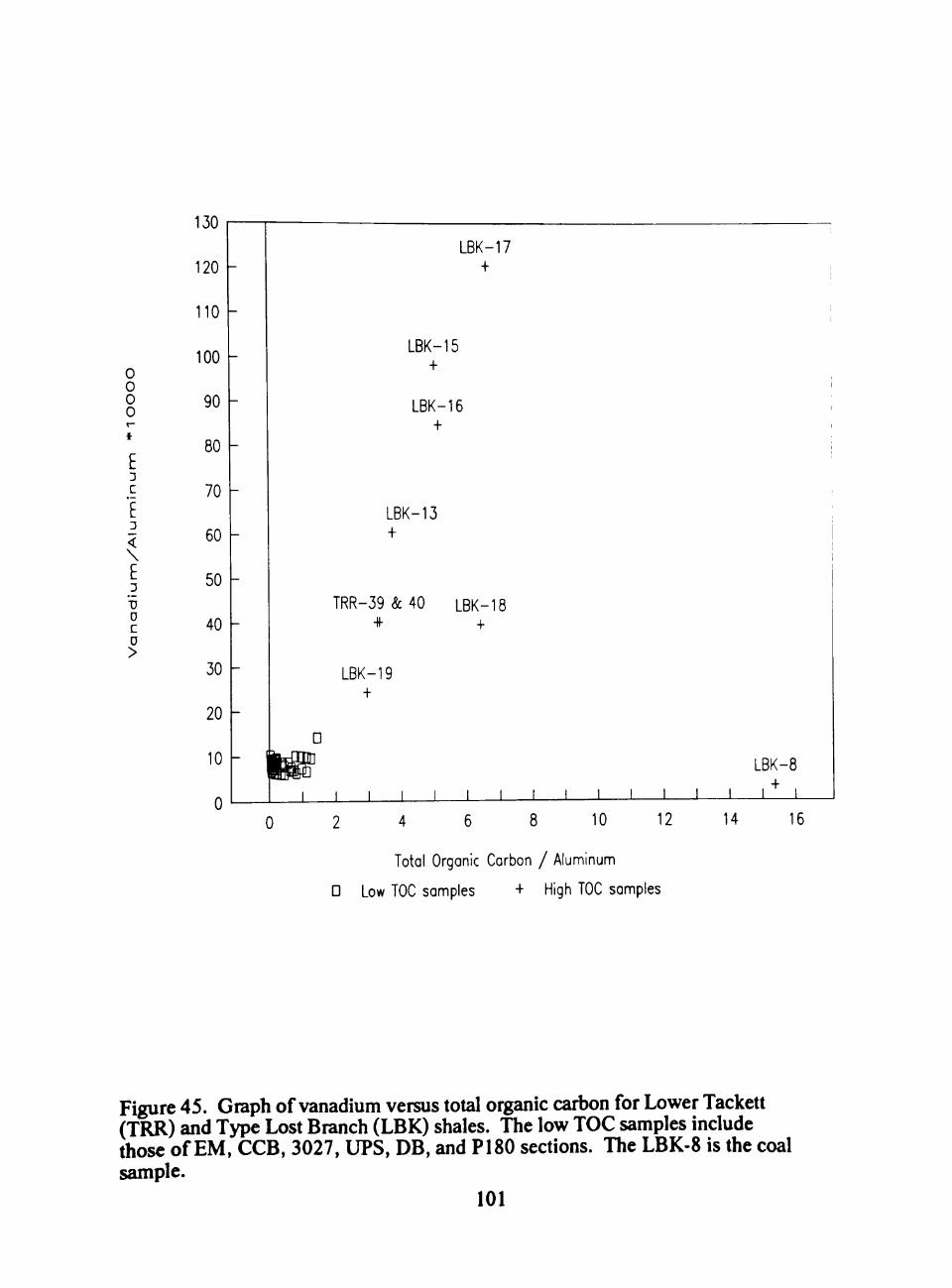
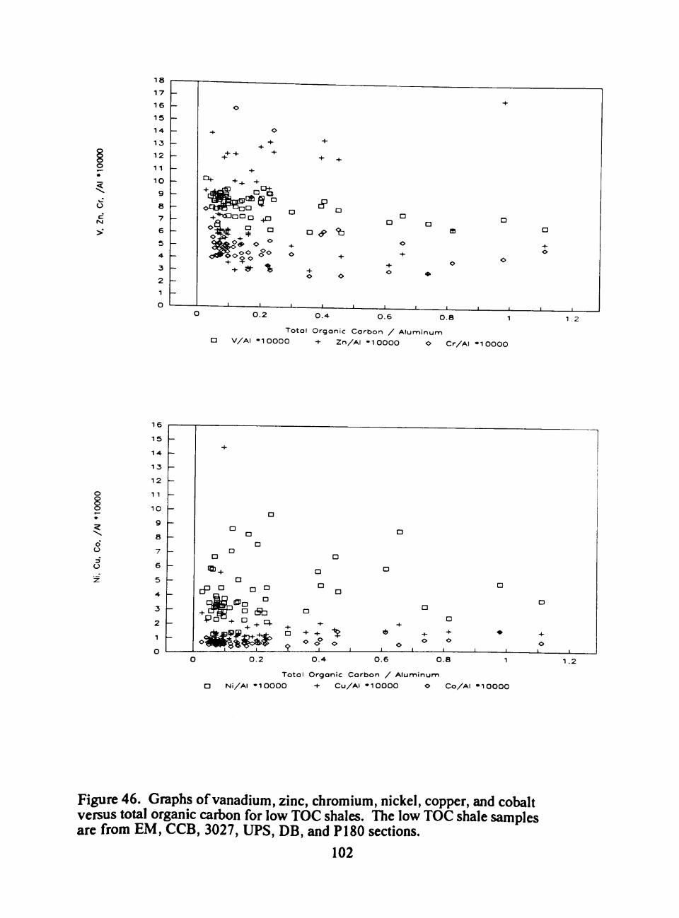
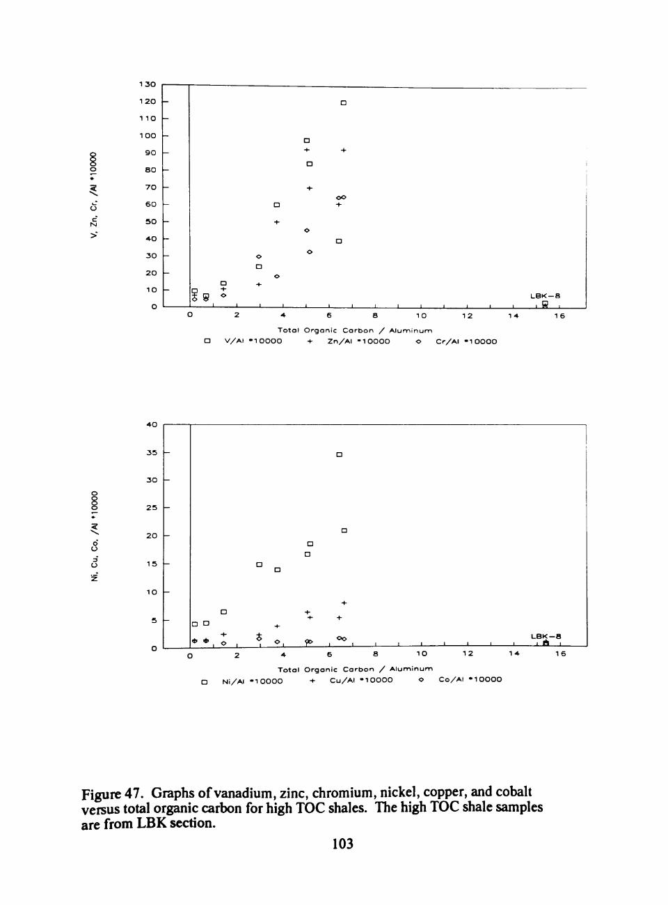
V. DISCUSSION 104
VI. CONCLUSIONS 110
REFERENCES 113
m
APPENDICES
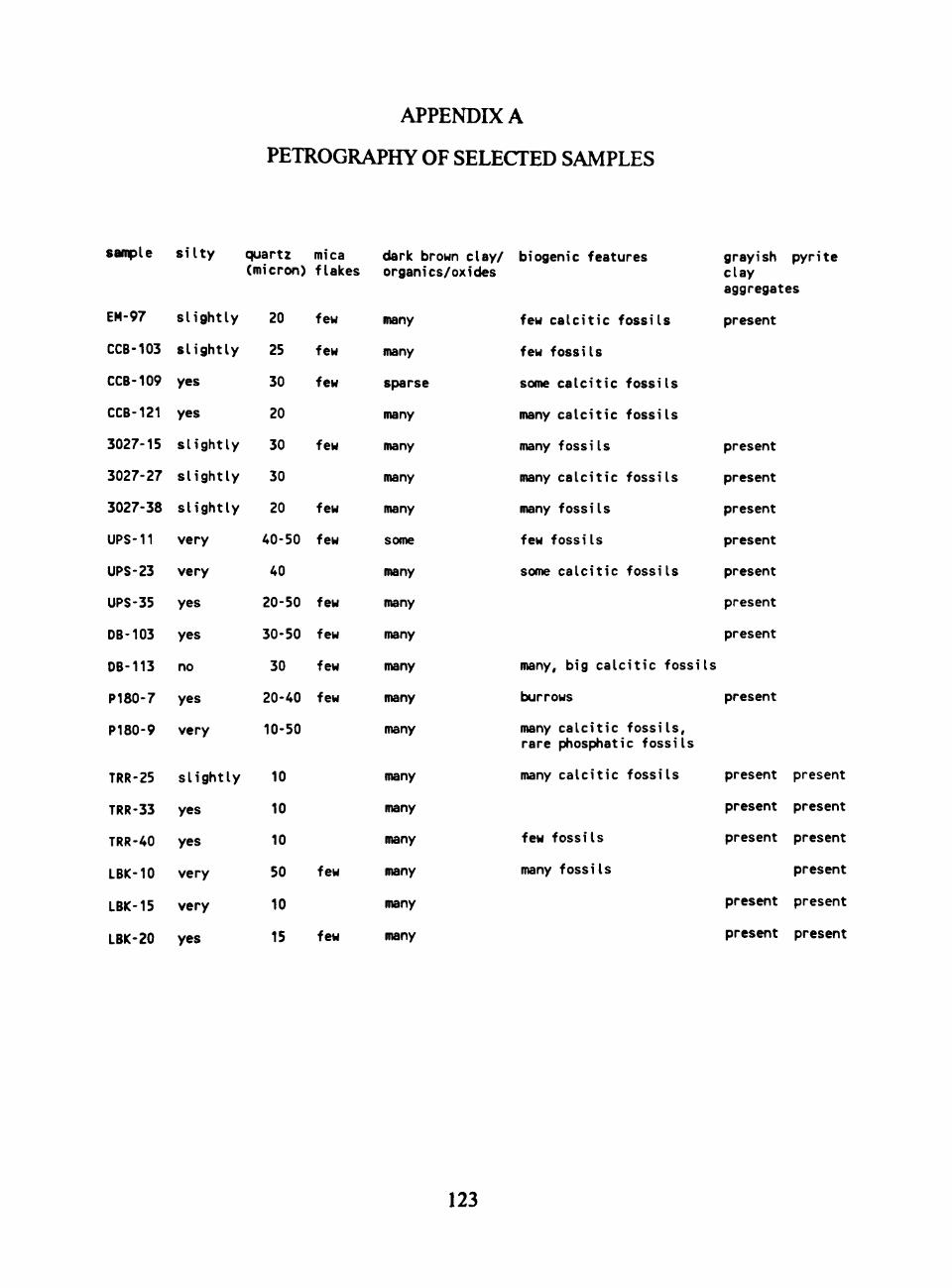
A. PETROGRAPHY OF SELECTED SAMPLES 123
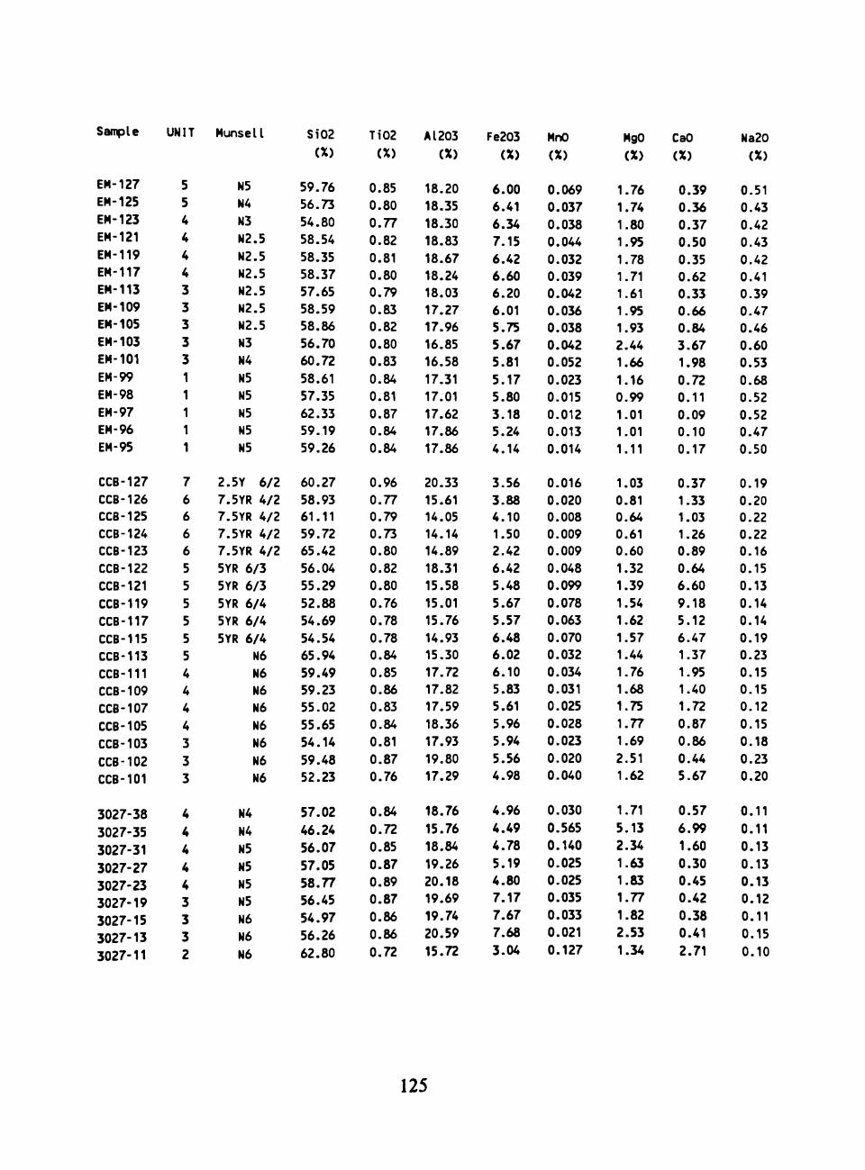
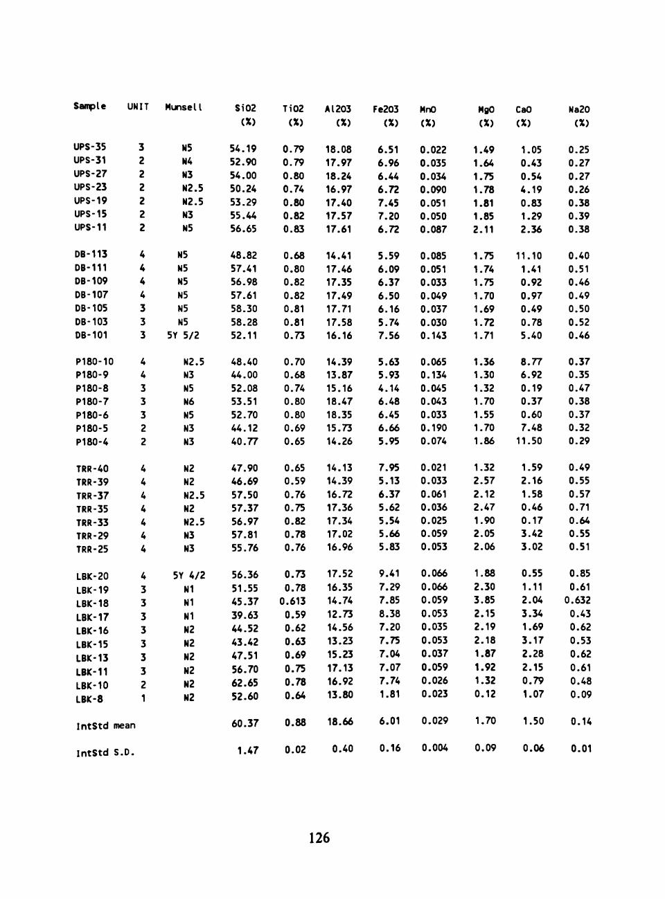
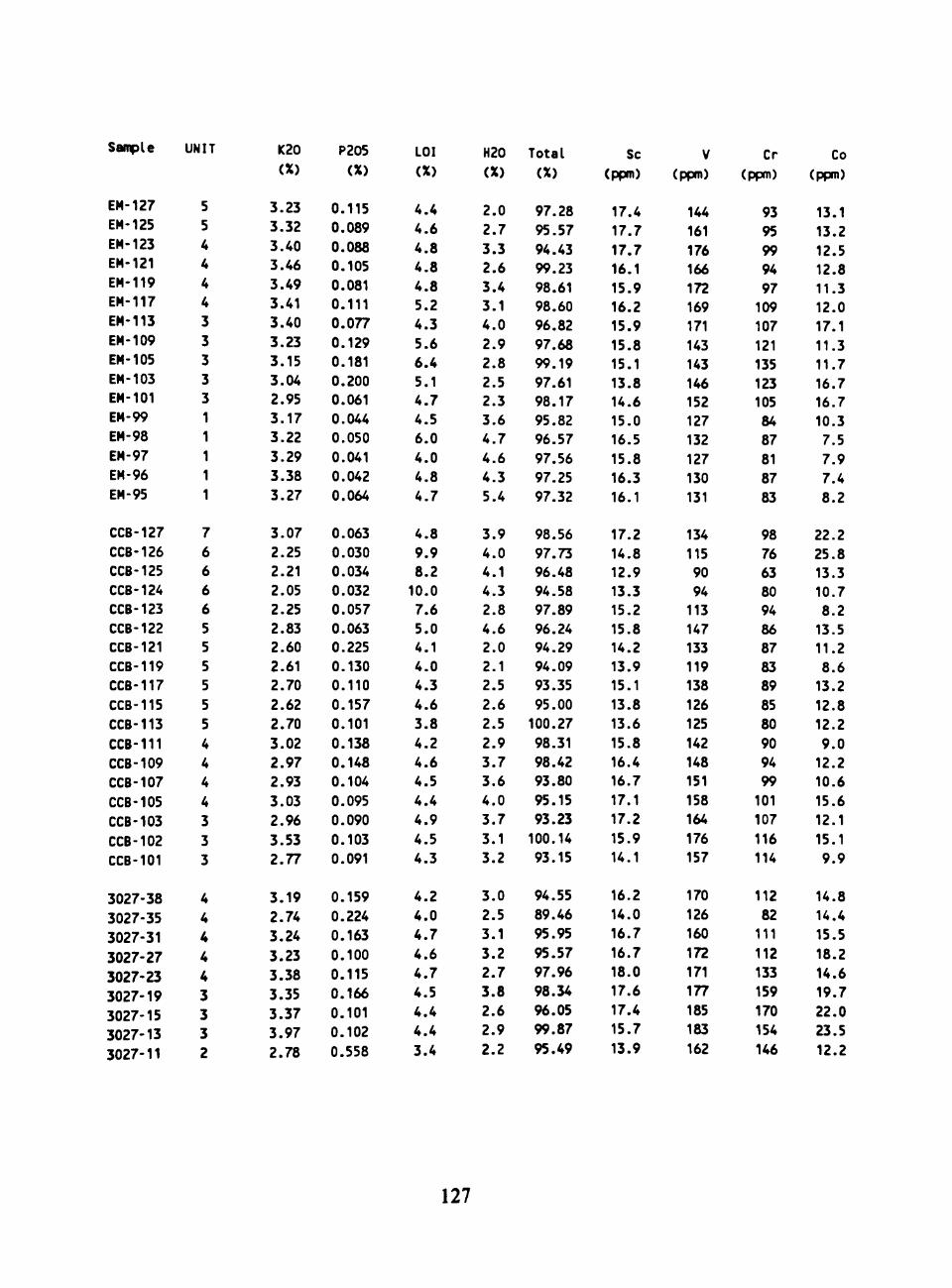
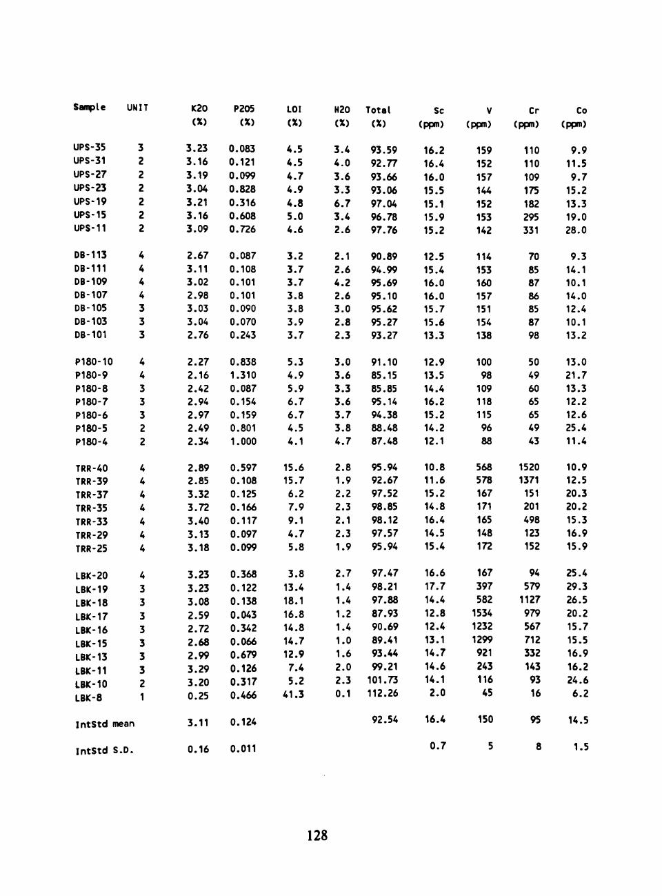
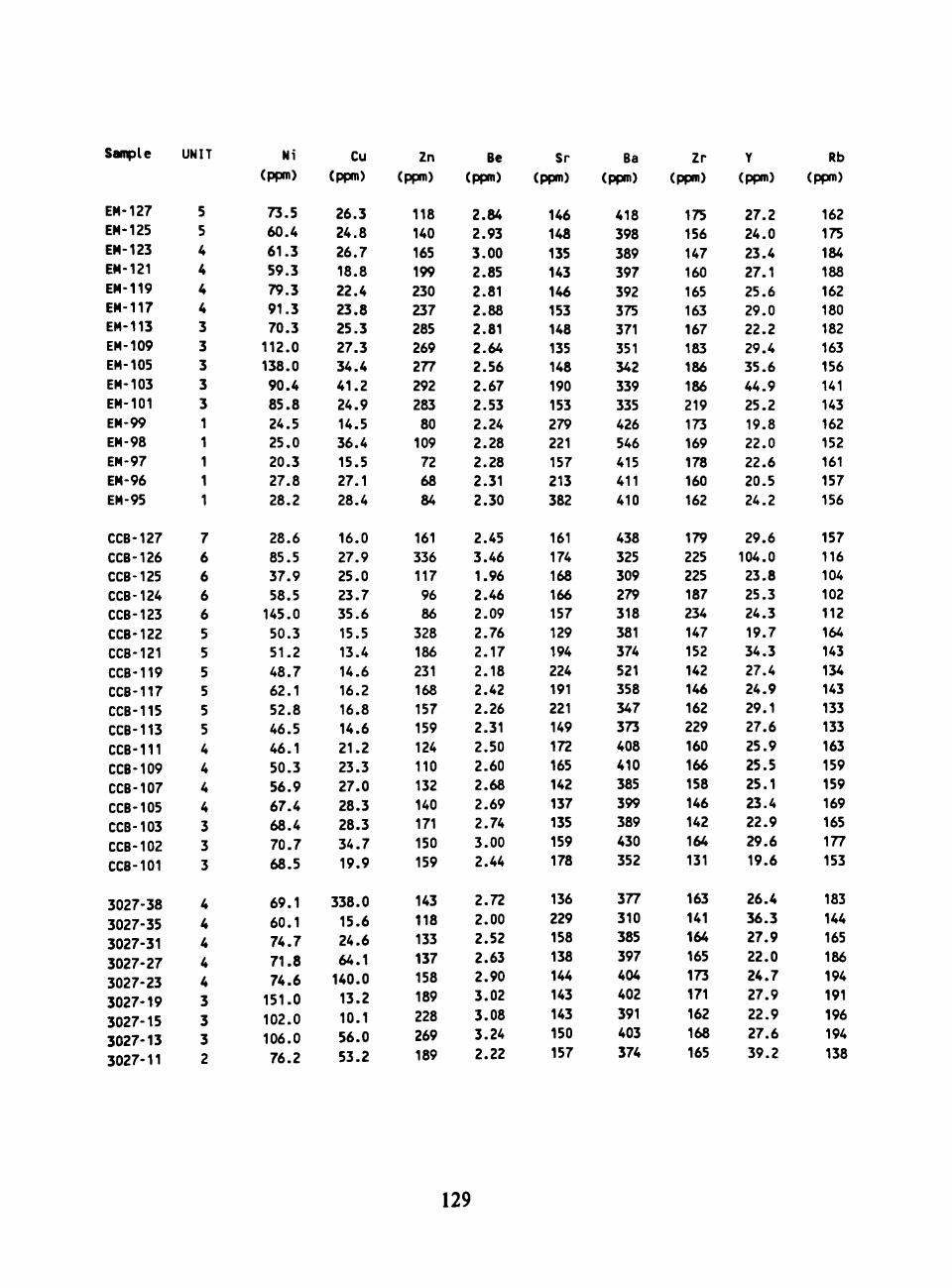
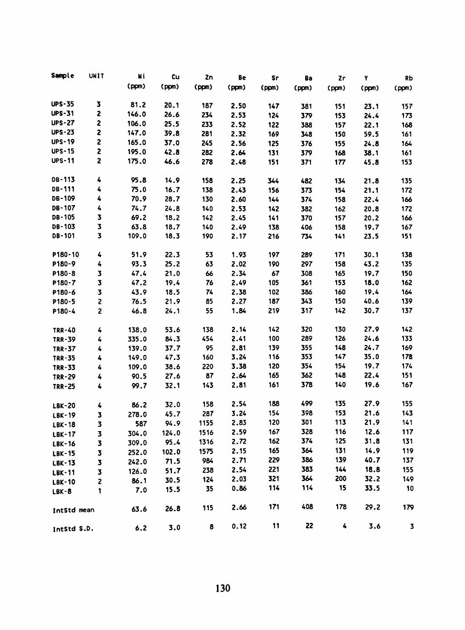
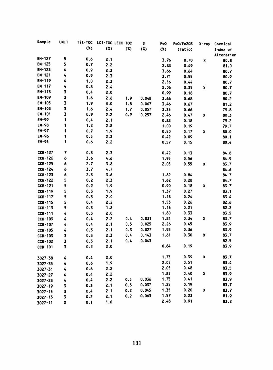
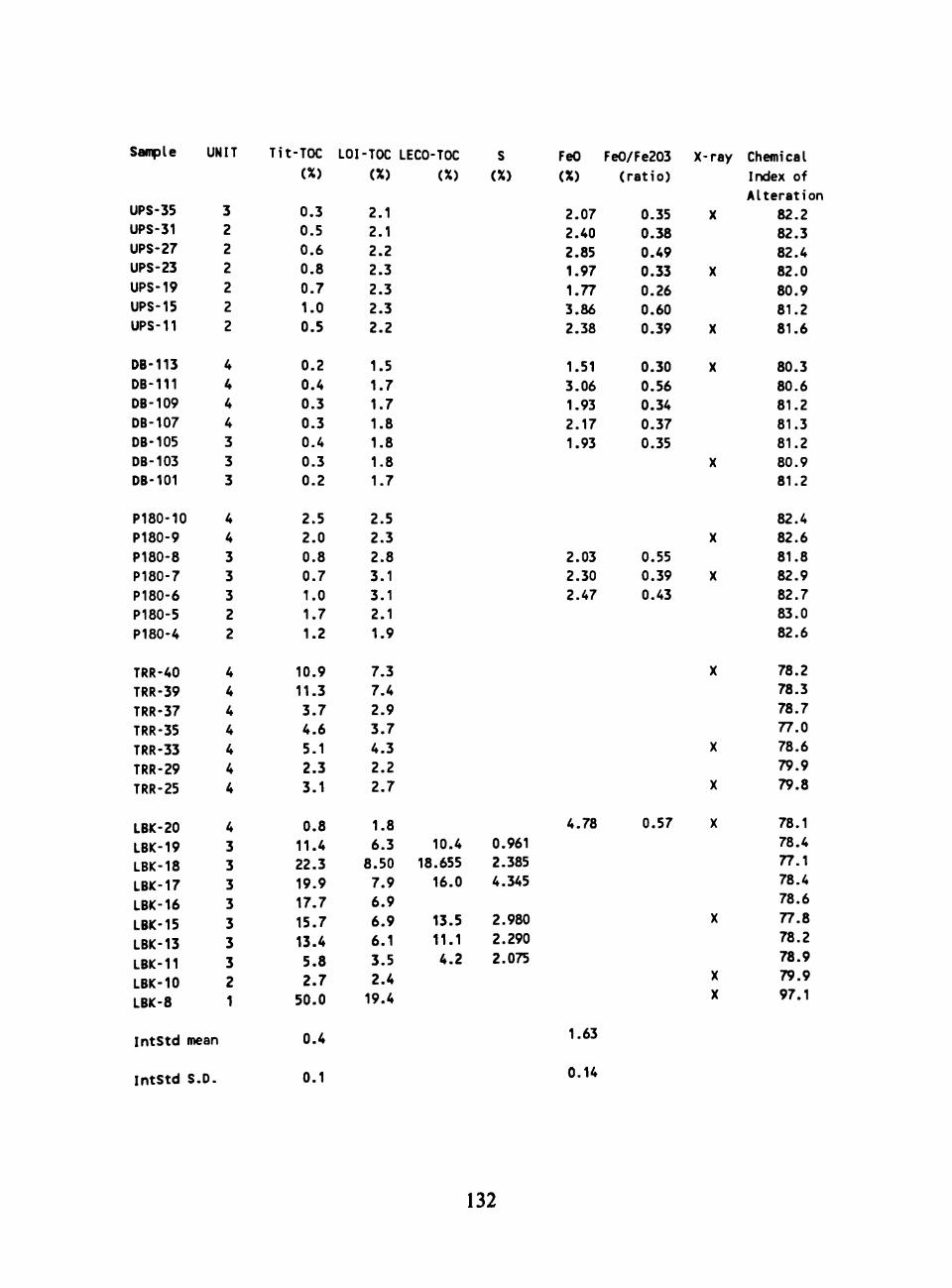
B. GEOCHEMICAL DATA 124
C. STRATIGRAPHIC DISTRIBUTION 133
IV
ABSTRACT
Pennsylvanian cyclothemic marine shales present a wide range of depositional
environments that allow the study of depositional controls on distribution of certain
elements in shales. Samples were collected from upper Desmoinesian to lower Virgilian
units in north-central Texas, Kansas, and Oklahoma, The samples were analyzed for
Si, Ti, Al, Fe, Mn, Mg, Ca, Na, K, P, Sc, V, Cr, Co, Ni, Cu, Zn, Be, Sr, Ba, Zr, Y,
Rb, S, and total organic carbon (TOC). X-ray diffraction showed that illite, kaolinite,
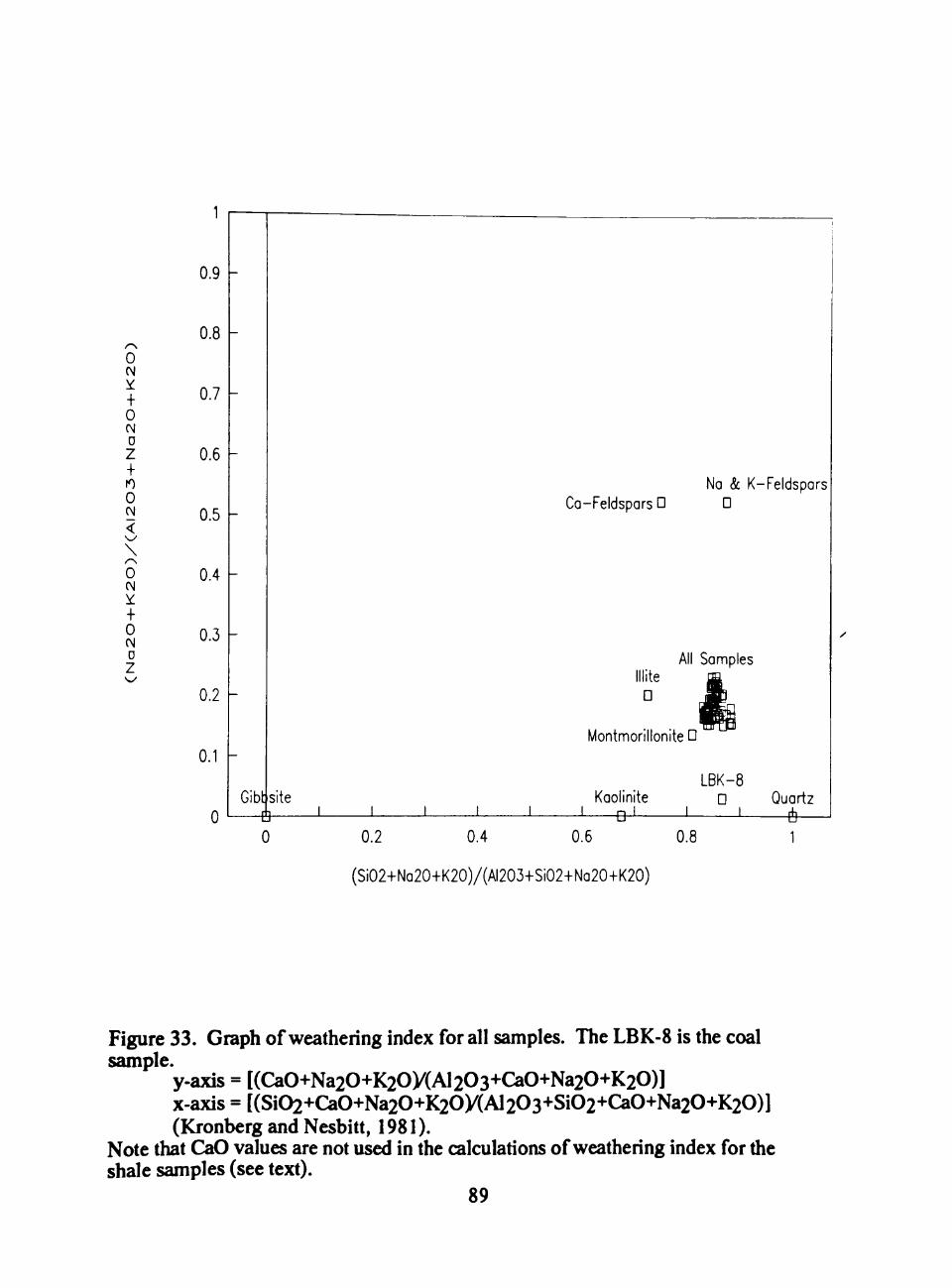
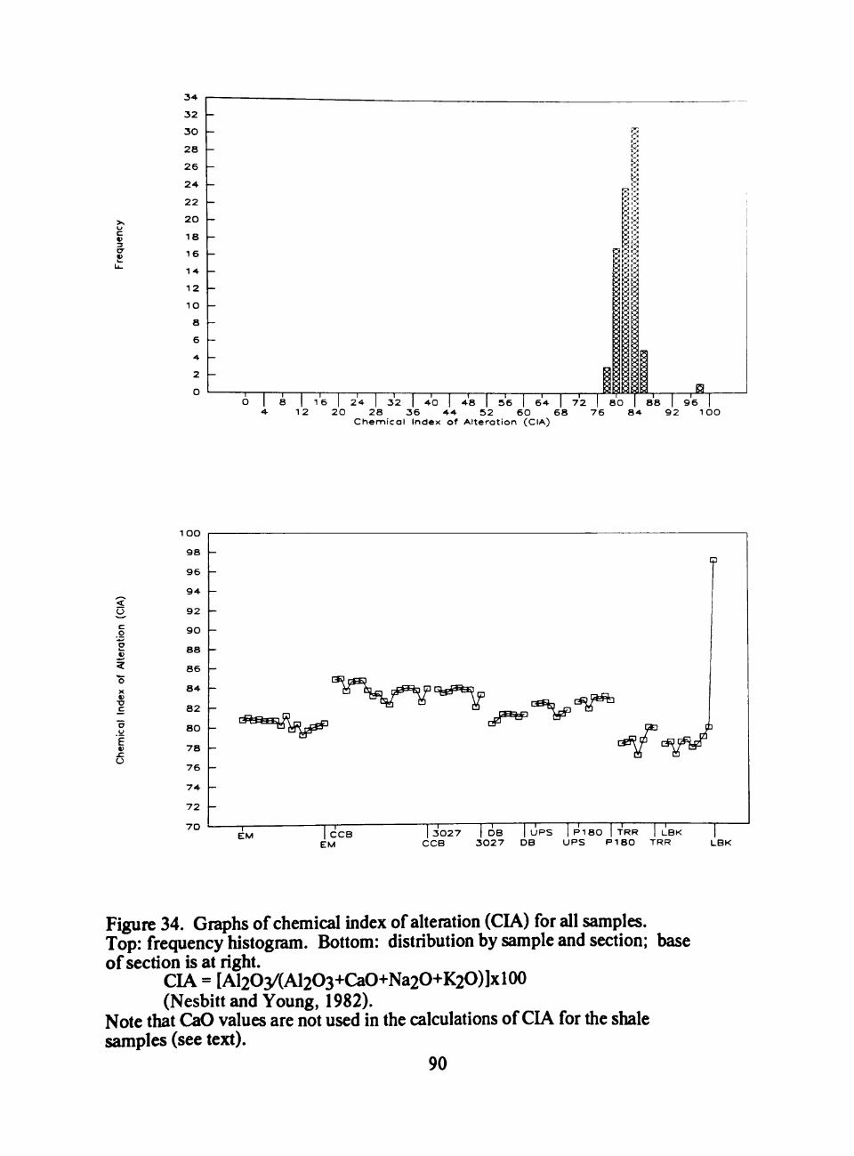
and quartz were the predominant minerals. The weathering index and the chemical
index of alteration both indicate that the source minerals of the shales were highly
weathered. Thin sections reveal the presence of red brown aggregates of clay, organics,
and oxides, gray clay aggregates, and quartz grains. Abundances of Mn and Fe are
quite variable (except for Mn in calcareous shales, and Fe in pyritic shales).
Core shales, deposited during maximum transgression, may be high or low TOC
shales depending on the original sedimentary redox conditions. In high TOC core
shales (TOC/Al ratio above 1.2), abundances of V, Zn, and Cr correlate strongly with
TOC. Sulfur correlates strongly with Fe. In low TOC core shales (TOC/Al ratio below
1.2), abundances of V, Zn, and Cr do not correlate with TOC. In some low TOC core
shales, Zn, Cr, Ni, and Cu increase in maximum transgressive intervals and decrease
stratigraphically upwards due to dilution by deltaic clays. Outside shales, deposited
during regression, are normal to marginal marine shales with low TOC. Carbonate-
related elements (Ca, Sr, Zn, Mn, P, Y, Ni) are more abundant where the shale contains
more calcareous skeletal material. Marginal marine shales show widely variable TOC
and elemental composition.
This study indicates that the main factors controlling the distribution of elements
in cyclothemic shales are (1) the degree of weathering before deposition, (2) redox
condition in the depositional environment, (3) settling time of the clay and organic matter
through the water colunm, (4) conditions conducive to the formation and deposition of
carbonates, (5) the composition of the organic matter, and (6) dilution by fine-grained
terrestrial sediments.
VI
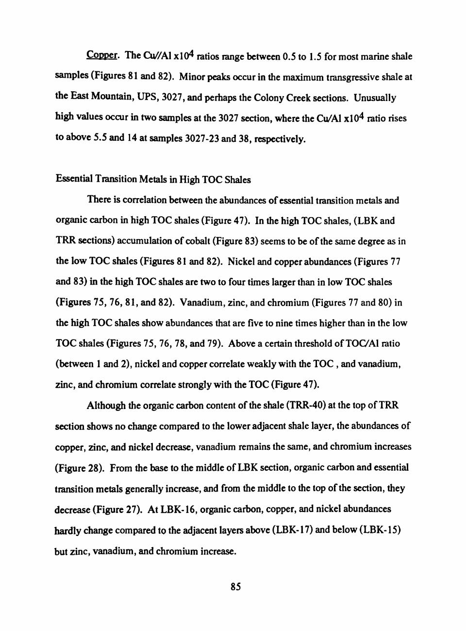
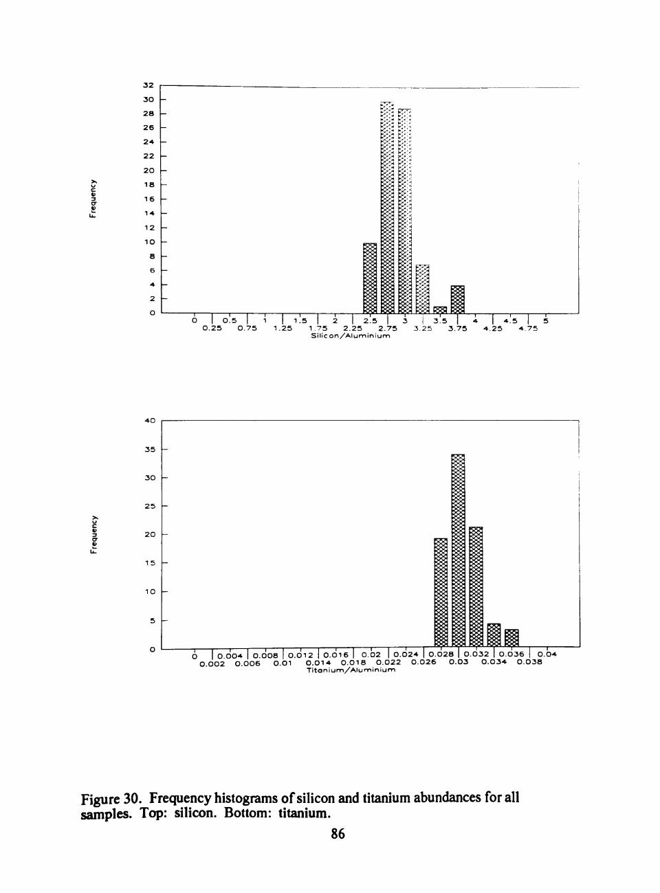
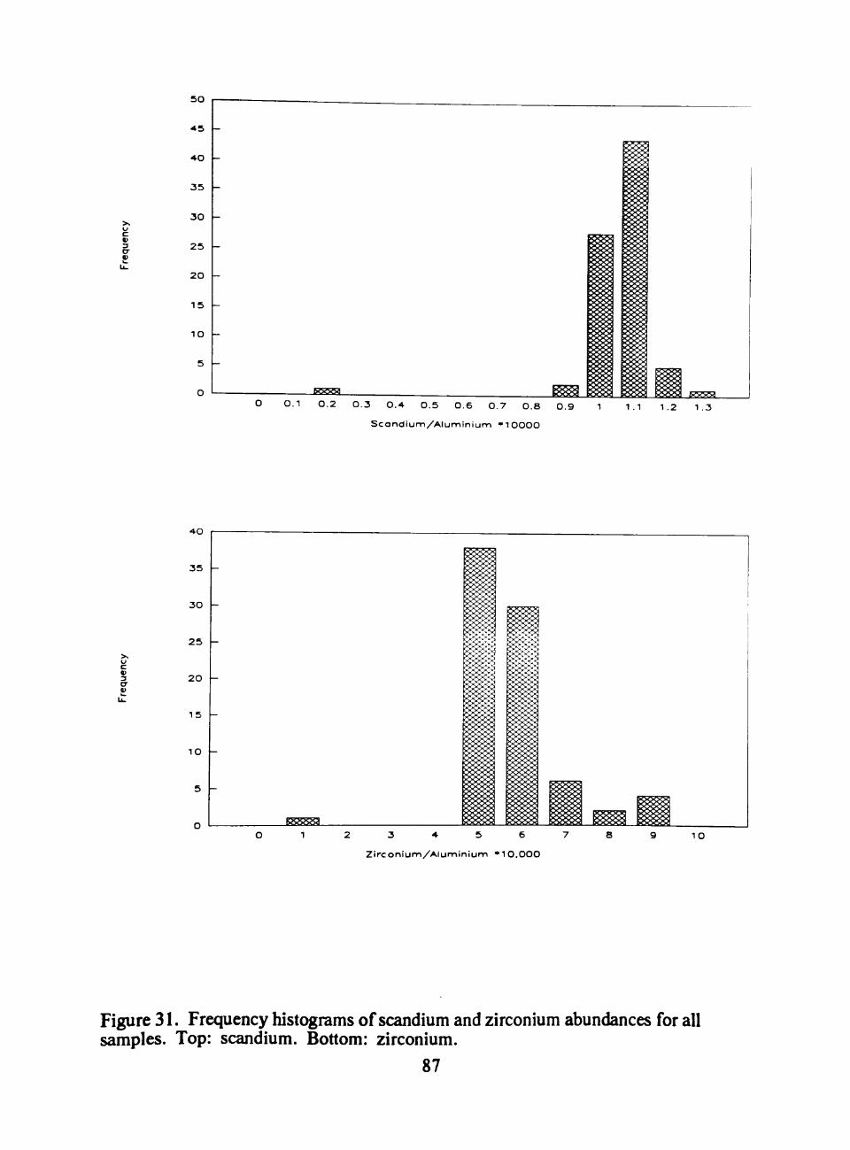
FIGURES
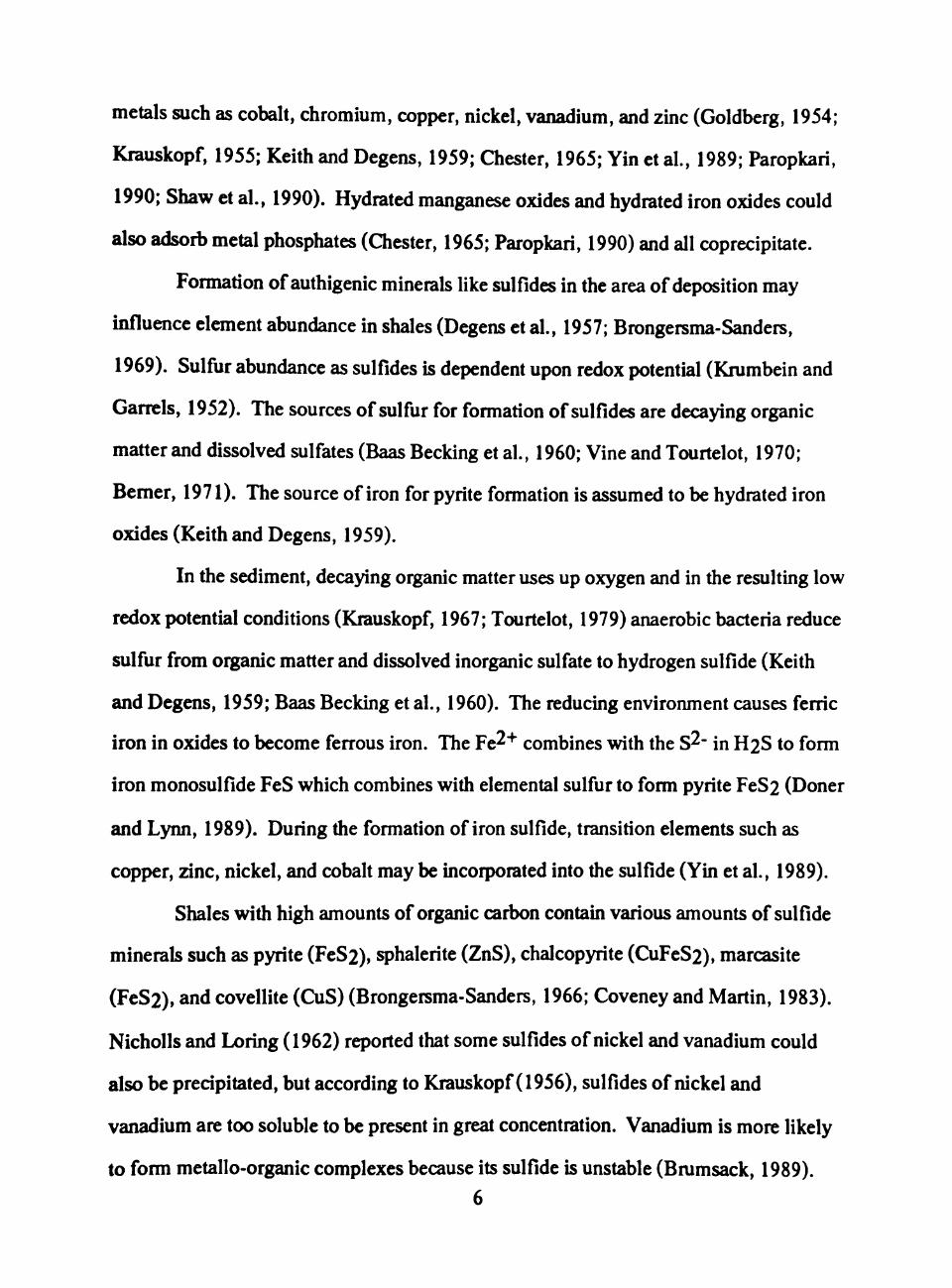
1. Basic vertical sequence of an individual Pennsylvanian cyclothem 13
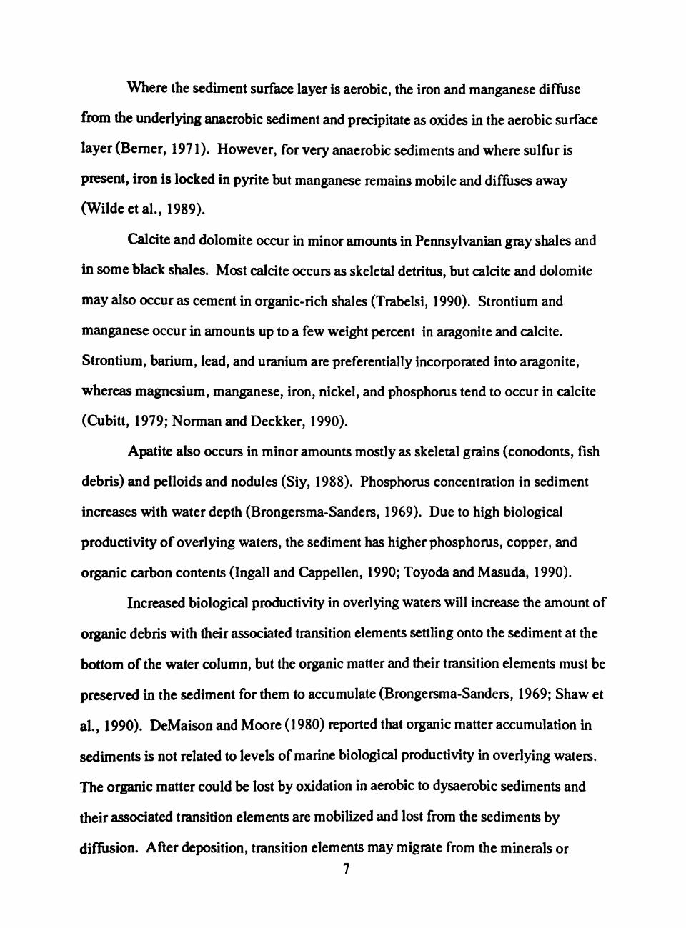
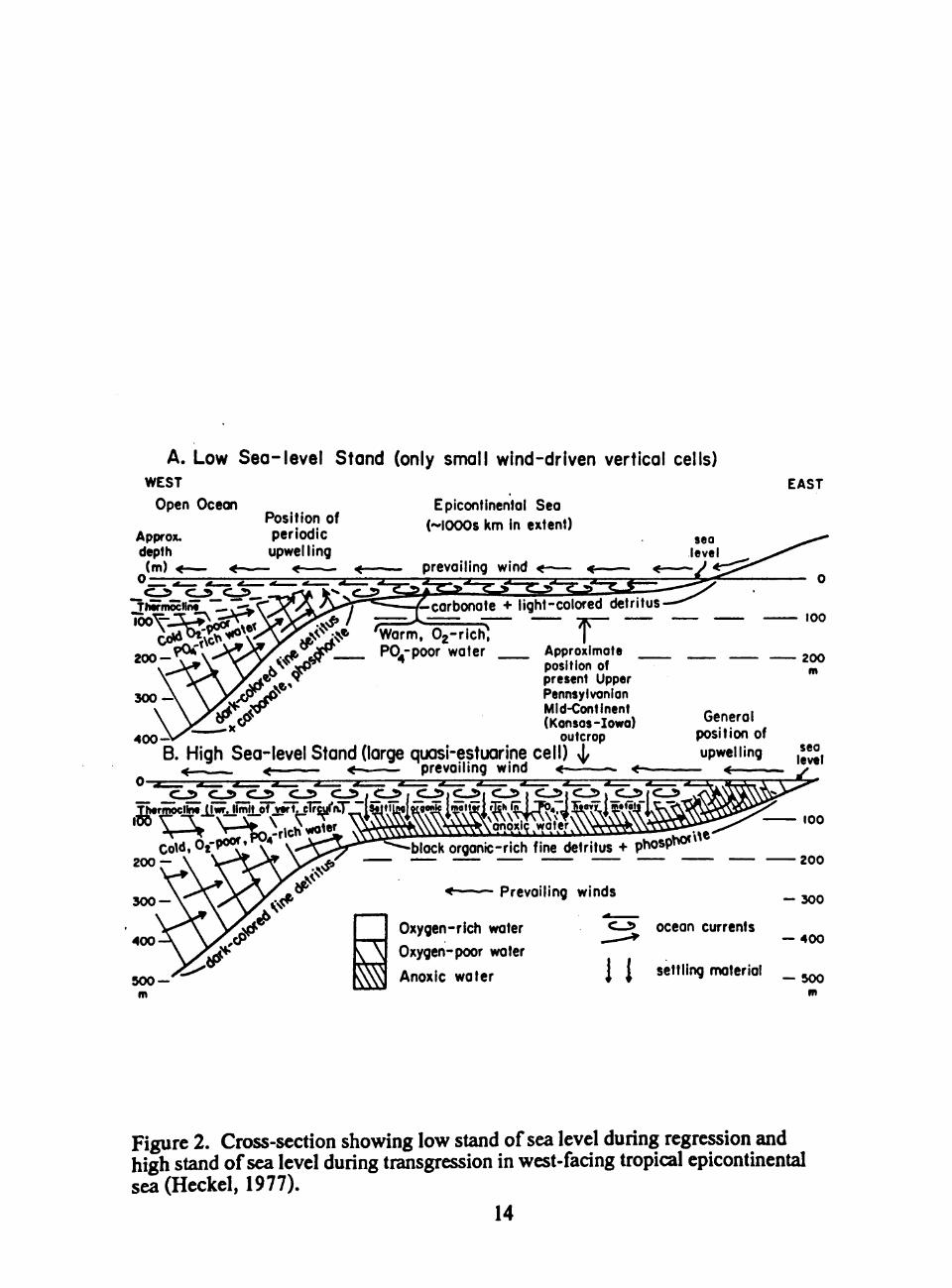
2. Cross-section showing low stand of sea level during regression and high stand of sea level during transgression in west-facing tropical epicontinental sea 14
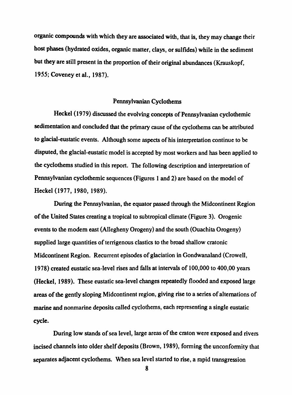
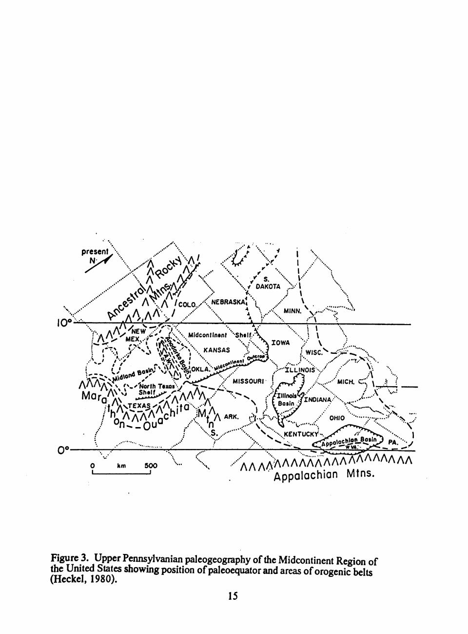
3. Upper Pennsylvanian paleogeography of the Midcontinent Region of the United States showing position of paleoequator and areas of orogenic belts 15
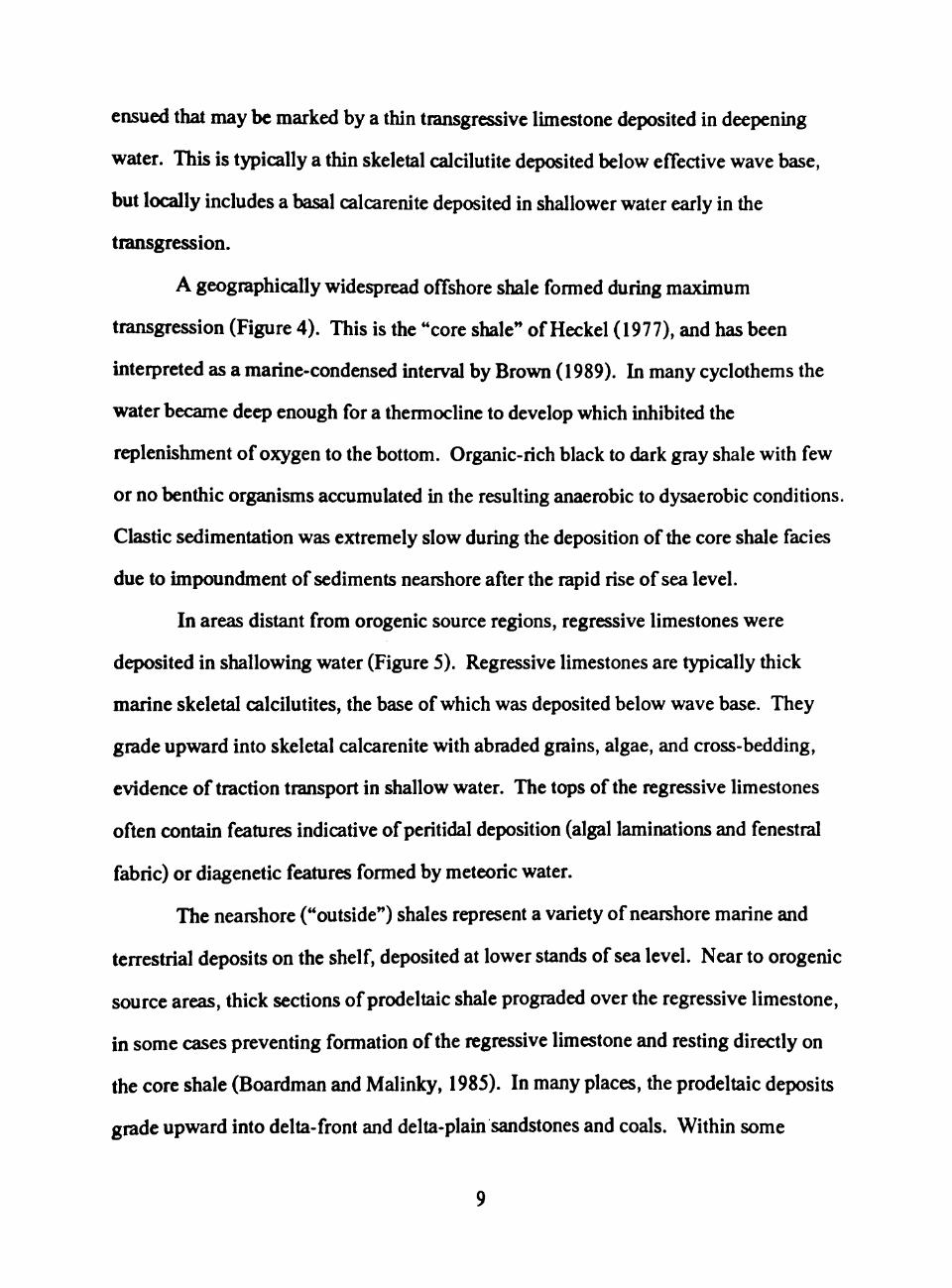
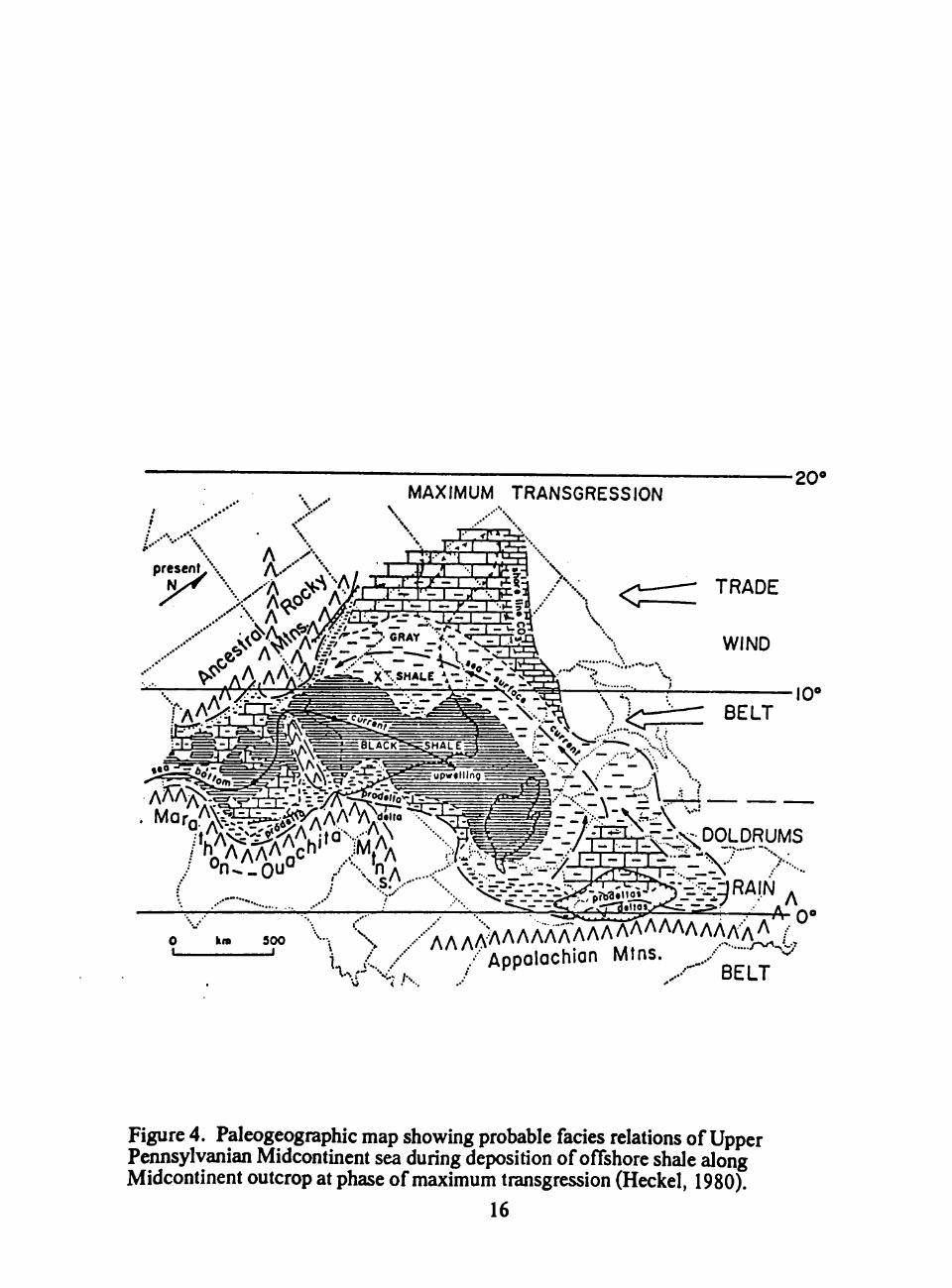
4. Paleogeographic map showing probable fades relations of Upper Pennsylvanian Midcontinent sea during deposition of offshore shale along Midcontinent outcrop at phase of maximum transgression 16
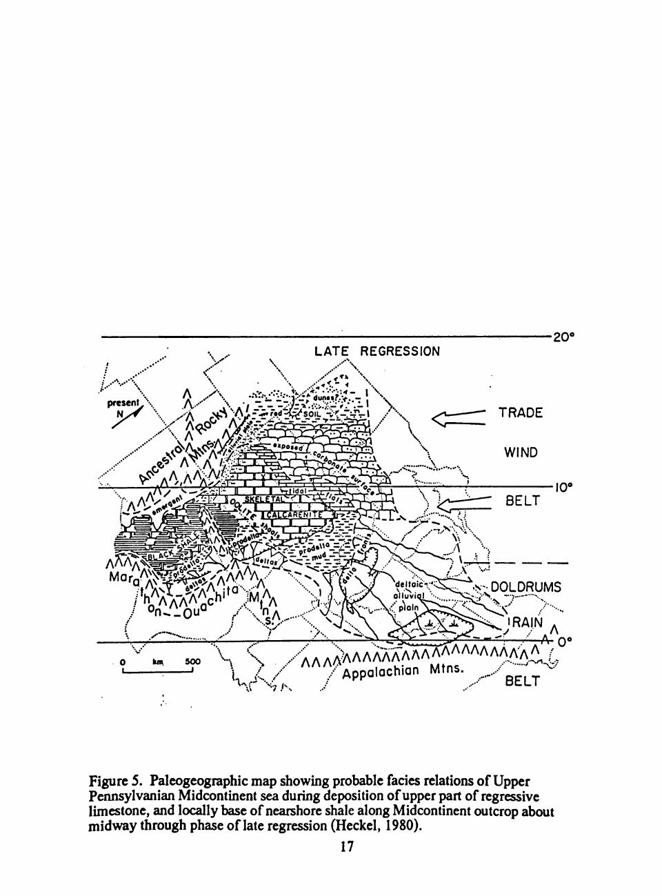
5. Paleogeographic map showing probable facies relations of Upper Permsylvanian Midcontinent sea during deposition of upper part of regressive limestone, and locally base of nearshore shale along Midcontinent outcrop about midway through phase of late regression 17
6. Distribution of Pennsylvanian strata in the Midcontinent Region of the United States 30
7. Eustatic sea-level curve for part of Pennsylvanian sequence in north-central Texas outcrop (right) and biostratigraphic correlation with curve forMidcontinent outcrop (left) 31
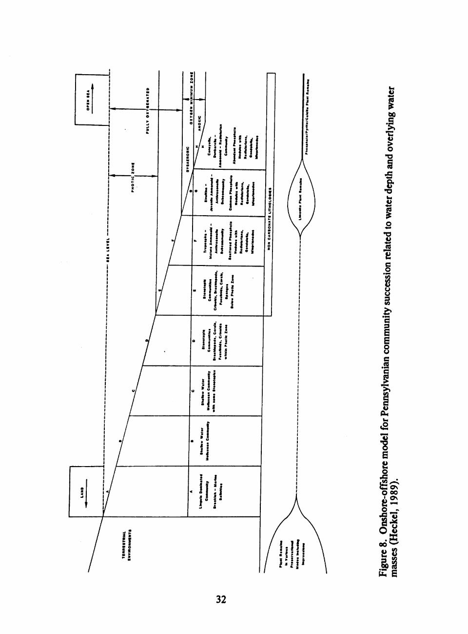
8. Onshore-offshore model for Pennsylvanian community succession related to water depth and overlying water masses 32
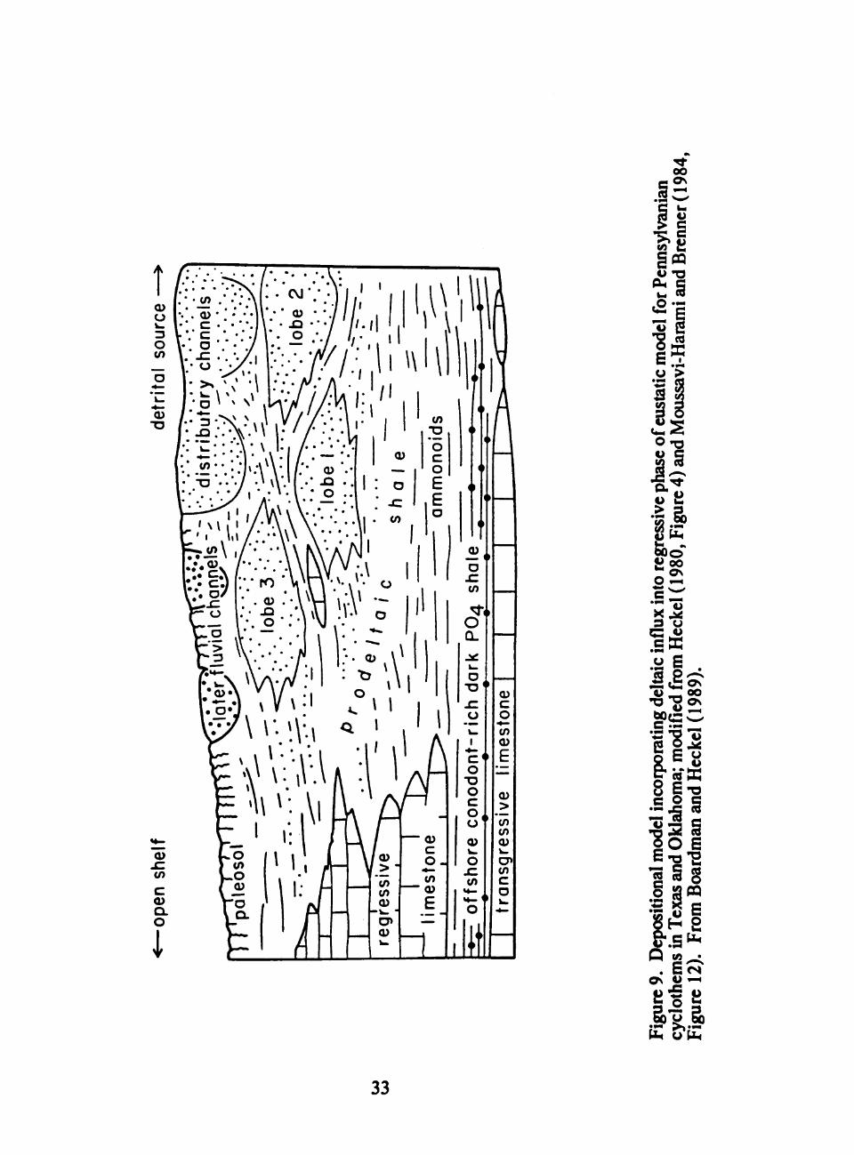
9. Depositional model incorporating deltaic influx into regressive phase of eustatic model for Pennsylvanian cyclothems in Texas and Oklahoma 33
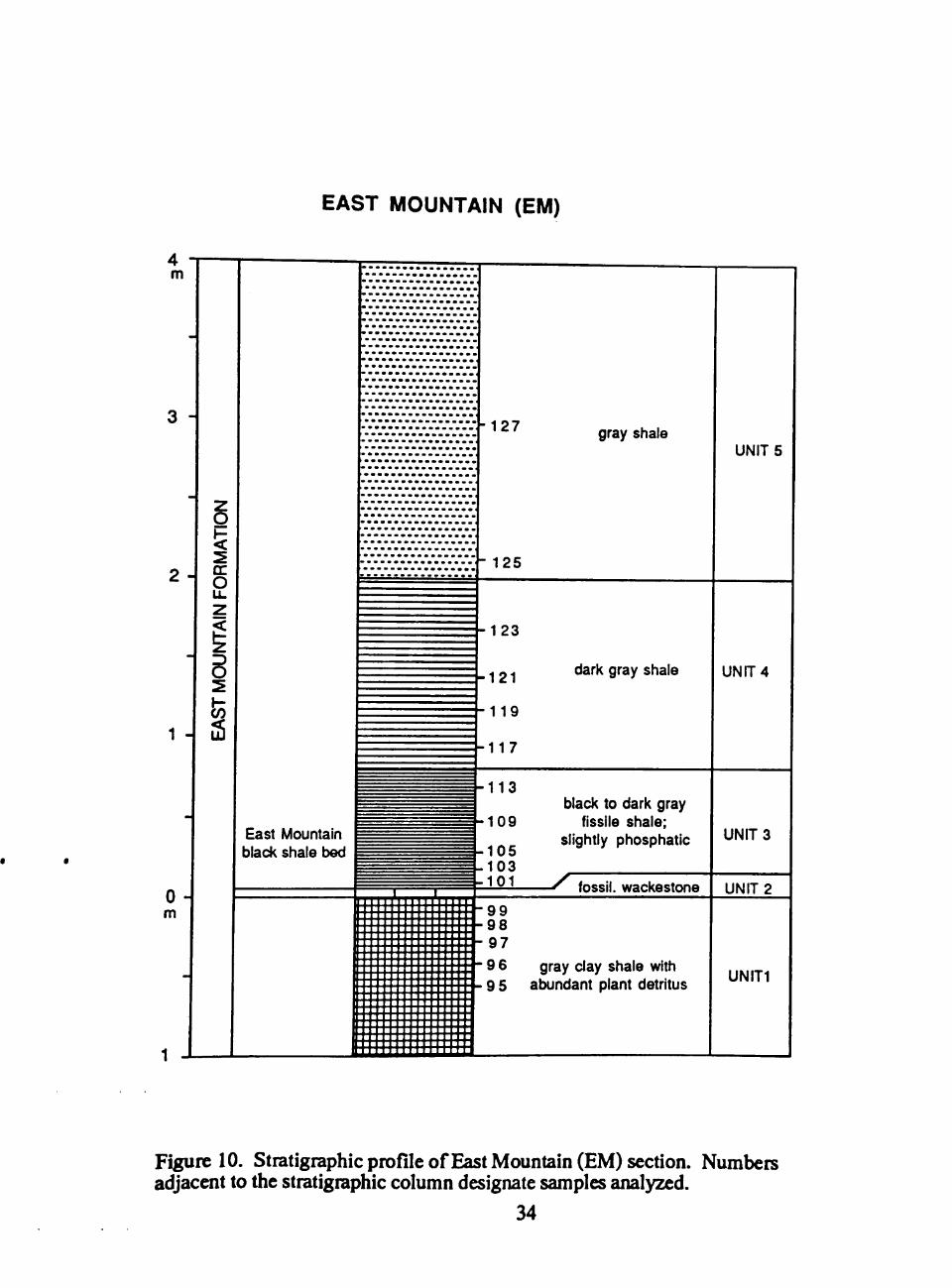
10. Stratigraphic profile of East Mountain (EM) section 34
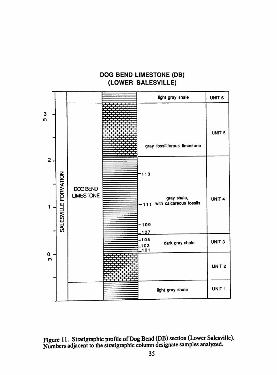
11. Stratigraphic profile of Dog Bend (DB) section (Lower Salesville) 35
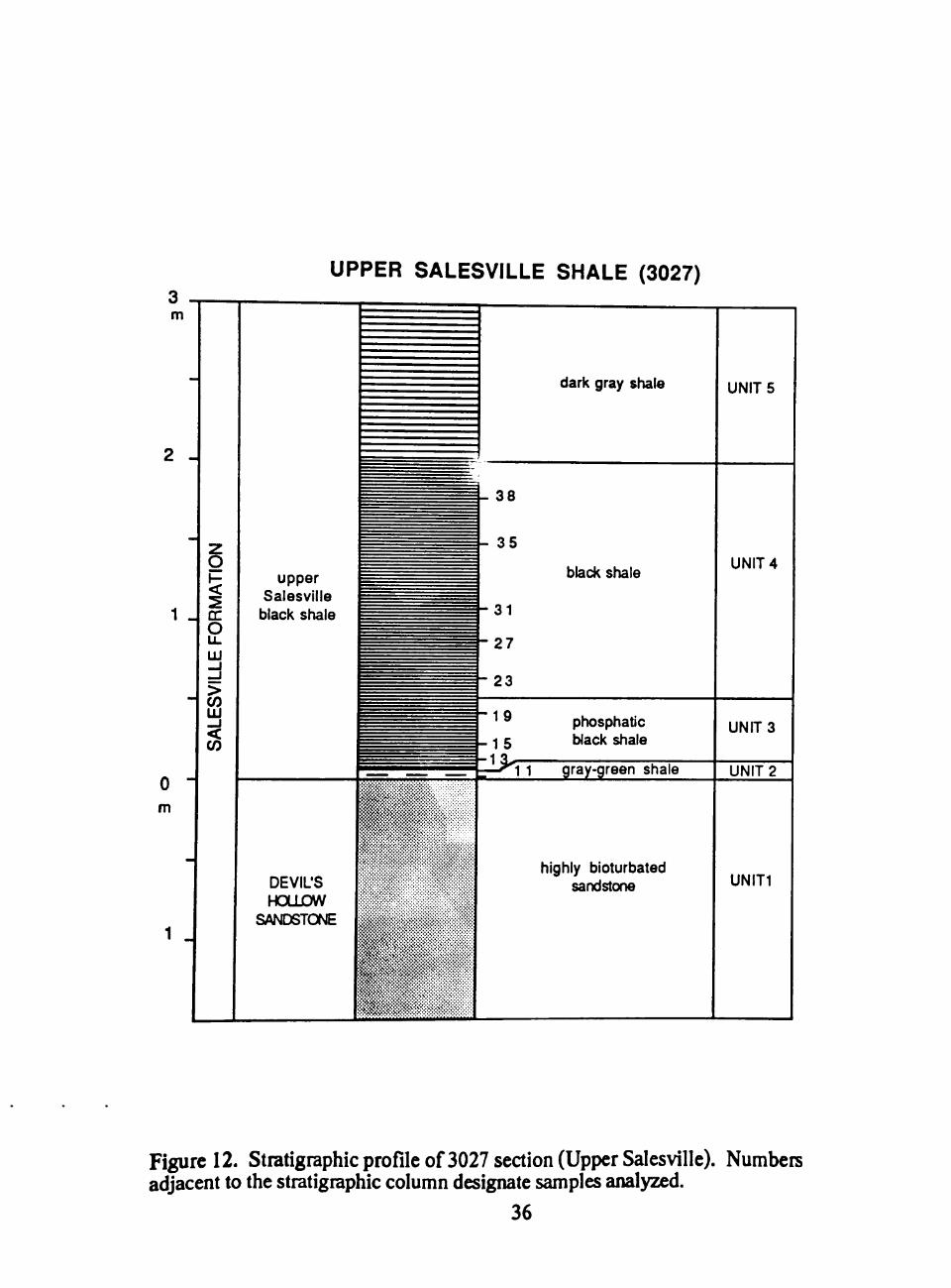
12. Stratigraphic profile of 3027 section (Upper Salesville) 36
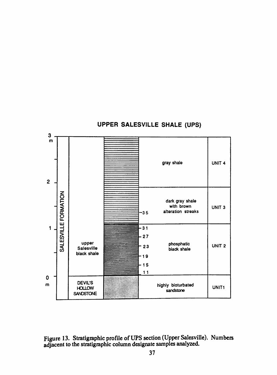
13. Stratigraphic profile of UPS section (Upper Salesville) 37
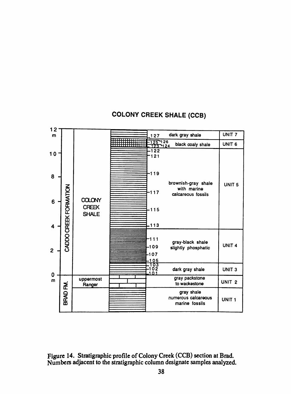
14. Stratigraphic profile of Colony Creek (CCB) section at Brad 38
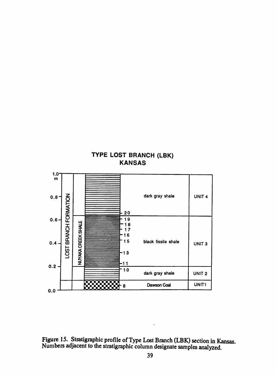
15. Stratigraphic profile of Type Lost Branch (LBK) section in Kansas 39
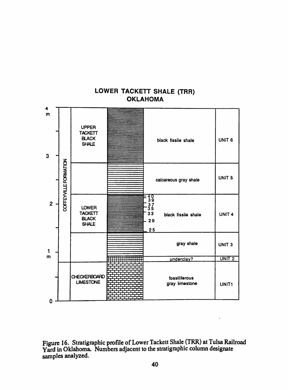
16. Stratigraphic profile of Lower Tackett Shale (TRR) at Tulsa Railroad Yard in Oklahoma 40
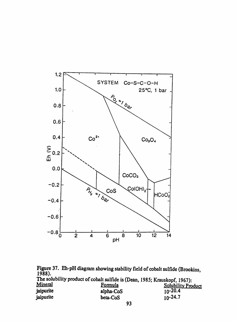
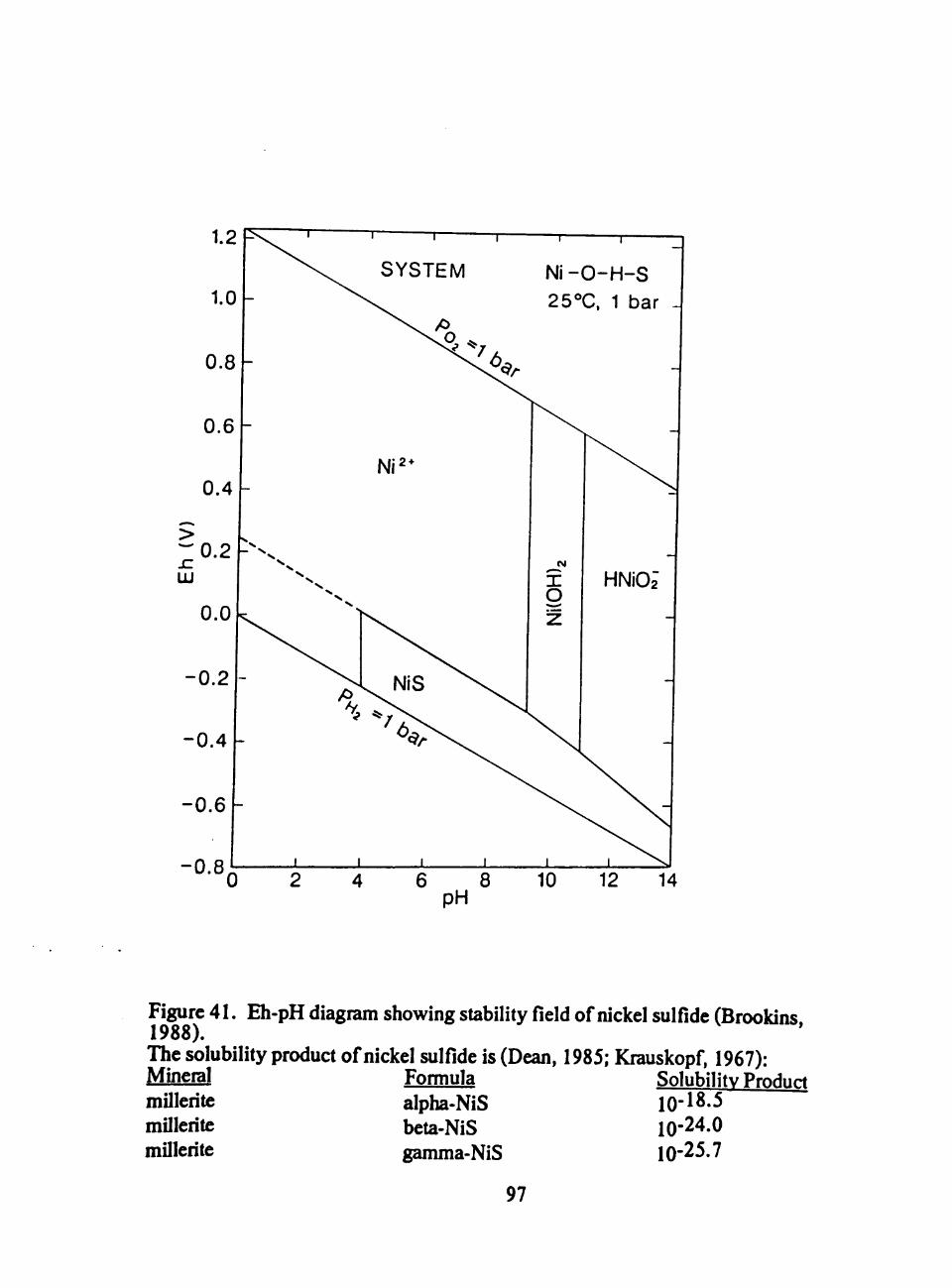
sulfur from oiganic matter and dissolved inorganic sulfate to hydrogen sulfide (Keith
and Degens, 1959; Baas Becking et al., 1960). The reducing environment causes ferric
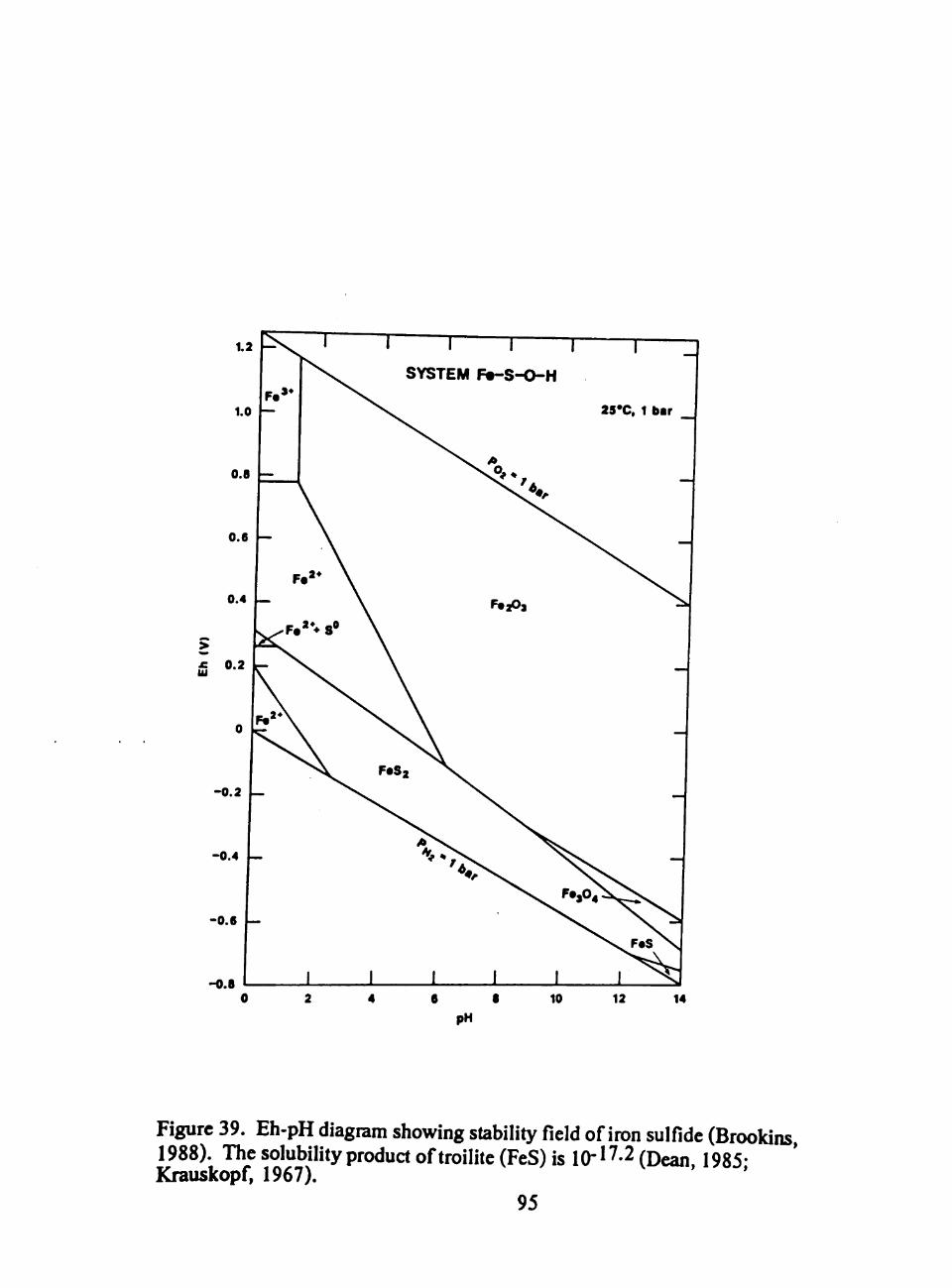
iron in oxides to become ferrous iron. The Fe2"'" combines with the S2- in H2S to form
iron monosulfide FeS which combines with elemental sulfur to form pyrite FeS2 (Doner
and Lynn, 1989). During the formation of iron sulfide, transition elements such as
copper, zinc, nickel, and cobalt may be incorporated into the sulfide (Yin et al., 1989).
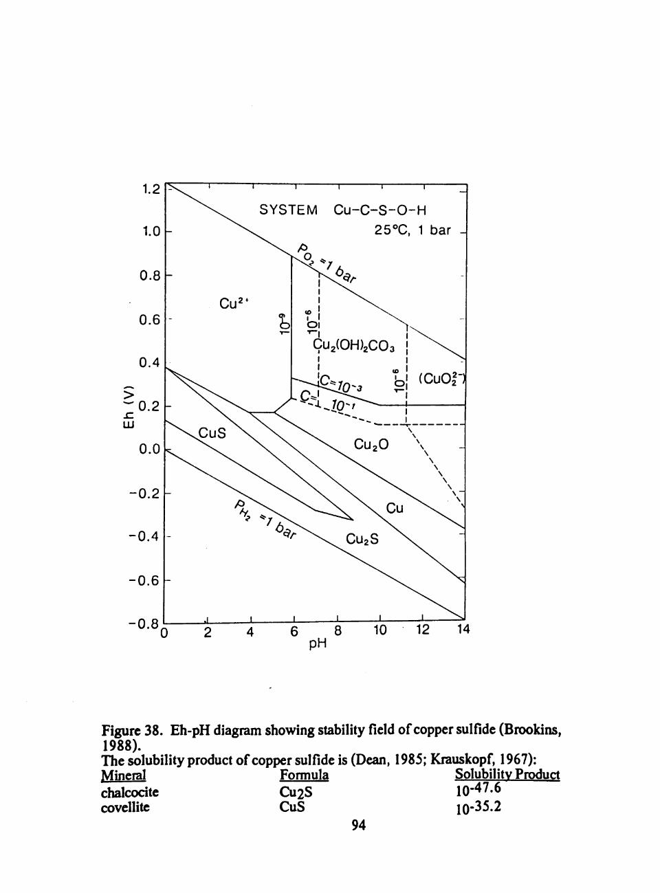
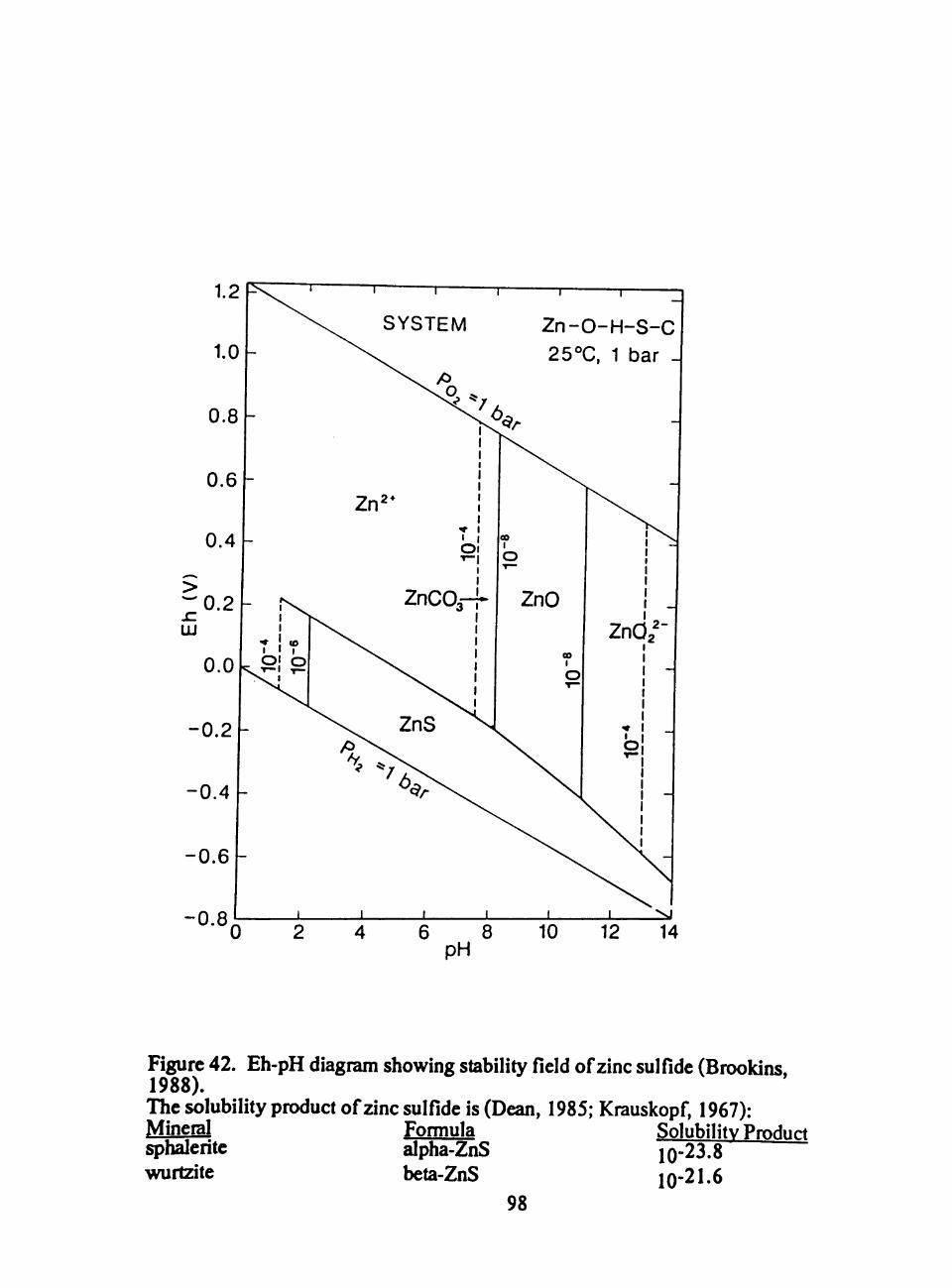
Shales with high amounts of organic carbon contain various amounts of sulfide
minerals such as pyrite (FeS2), sphalerite (ZnS), chalcopyrite (CuFeS2), marcasite
(FeS2), and covellite (CuS) (Brongersma-Sanders, 1966; Coveney and Martin, 1983).
Nicholls and Loring (1962) reported that some sulfides of nickel and vanadium could
also be precipitated, but according to Krauskopf (1956), sulfides of nickel and
vanadium are too soluble to be present in great concentration. Vanadium is more likely
to form metallo-organic complexes because its sulfide is unstable (Brumsack, 1989). 6
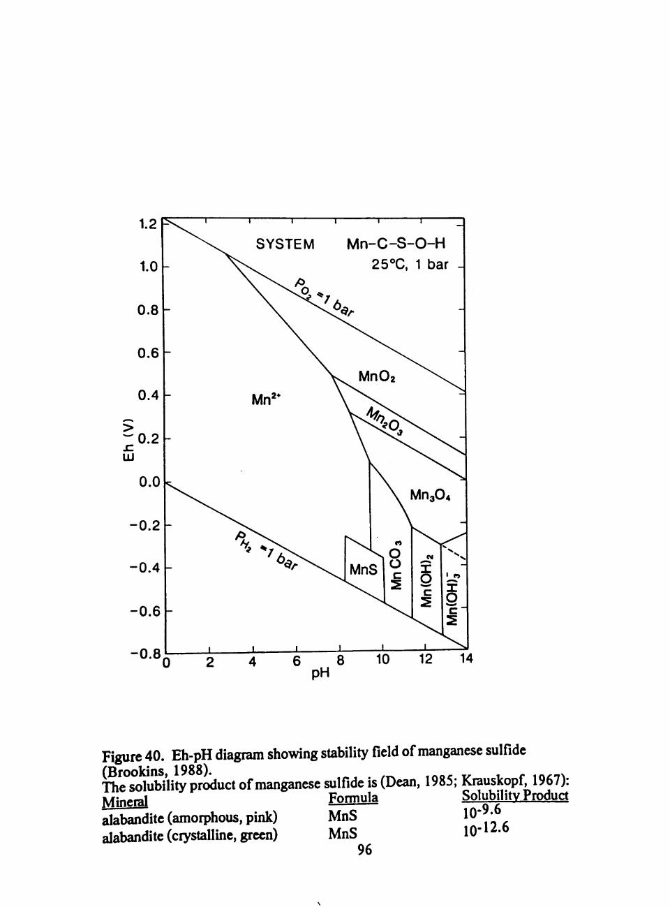
Where the sediment surface layer is aerobic, the iron and manganese difluse
from the underlying anaerobic sediment and precipitate as oxides in the aerobic surface
layer (Bemer, 1971). However, for very anaerobic sediments and where sulfur is
present, iron is locked in pyrite but manganese remains mobile and diffuses away
(Wilde etal., 1989).
Calcite and dolomite occur in minor amounts in Pennsylvanian gray shales and
in some black shales. Most calcite occurs as skeletal detritus, but calcite and dolomite
may also occur as cement in organic-rich shales (Trabelsi, 1990). Strontium and
manganese occur in amounts up to a few weight percent in aragonite and calcite.
Strontium, barium, lead, and uranium are preferentially incorporated into aragonite,
whereas magnesium, manganese, iron, nickel, and phosphorus tend to occur in calcite
(Cubitt, 1979; Norman and Deckker, 1990).
Apatite also occurs in minor amounts mostly as skeletal grains (conodonts, fish
debris) and pelloids and nodules (Siy, 1988). Phosphorus concentration in sediment
increases with water depth (Brongersma-Sanders, 1969). Due to high biological
productivity of overlying waters, the sediment has higher phosphorus, copper, and
oi;ganic carbon contents (Ingall and Cappellen, 1990; Toyoda and Masuda, 1990).
Increased biological productivity in overlying waters will increase the amount of
organic debris with their associated transition elements settling onto the sediment at the
bottom of the water column, but the organic matter and their transition elements must be
preserved in the sediment for them to accumulate (Brongersma-Sanders, 1969; Shaw et
al., 1990). DeMaison and Moore (1980) reported that organic matter accumulation in
sediments is not related to levels of marine biological productivity in overlying waters.
The organic matter could be lost by oxidation in aerobic to dysaerobic sediments and
their associated transition elements are mobilized and lost from the sediments by
diffusion. After deposition, transition elements may migrate from the minerals or 7
organic compounds with which they are associated with, that is, they may change their
host phases (hydrated oxides, organic matter, clays, or sulfides) while in the sediment
but they are still present in the proportion of their original abundances (Krauskopf,
1955; Coveney etal., 1987).
Pennsylvanian Cyclothems
Heckel (1979) discussed the evolving concepts of Pennsylvanian cyclothemic
sedimentation and concluded that the primary cause of the cyclothems can be attributed
to glacial-eustatic events. Although some aspects of his interpretation continue to be
disputed, the glacial-eustatic model is accepted by most workers and has been applied to
the cyclothems studied in this report. The following description and interpretation of
Pennsylvanian cyclothemic sequences (Figures 1 and 2) are based on the model of
Heckel (1977, 1980, 1989).
During the Pennsylvanian, the equator passed through the Midcontinent Region
of the United States creating a tropical to subtropical climate (Figure 3). Orogenic
events to the modem east (Allegheny Orogeny) and the south (Ouachita Orogeny)
supplied large quantities of terrigenous elastics to the broad shallow cratonic
Midcontinent Region. Recurrent episodes of glaciation in Gondwanaland (Crowell,
1978) created eustatic sea-level rises and falls at intervals of 100,000 to 400,00 years
(Heckel, 1989). These eustatic sea-level changes repeatedly flooded and exposed large
areas of the gently sloping Midcontinent region, giving rise to a series of alternations of
marine and nonmarine deposits called cyclothems, each representing a single eustatic
cycle.
During low stands of sea level, large areas of the craton were exposed and rivers
incised charmels into older shelf deposits (Brown, 1989), forming the unconformity that
separates adjacent cyclothems. When sea level started to rise, a rapid transgression 8
ensued that may be marked by a thin transgressive limestone deposited in deepening
water. This is typically a thin skeletal calcilutite deposited below effective wave base,
but locally includes a basal calcarenite deposited in shallower water early in the
transgression.
A geographically widespread offshore shale formed during maximum
transgression (Figure 4). This is the "core shale** of Heckel (1977), and has been
interpreted as a marine-condensed interval by Brown (1989). In many cyclothems the
water became deep enough for a thermocline to develop which inhibited the
replenishment of oxygen to the bottom. Organic-rich black to dark gray shale with few
or no benthic organisms accumulated in the resulting anaerobic to dysaerobic conditions.
Clastic sedimentation was extremely slow during the deposition of the core shale facies
due to impoundment of sediments nearshore after the rapid rise of sea level.
In areas distant from orogenic source regions, regressive limestones were
deposited in shallowing water (Figure 5). Regressive limestones are typically thick
marine skeletal calcilutites, the base of which was deposited below wave base. They
grade upward into skeletal calcarenite with abraded grains, algae, and cross-bedding,
evidence of traction transport in shallow water. The tops of the regressive limestones
often contain features indicative of peritidal deposition (algal laminations and fenestral
fabric) or diagenetic features formed by meteoric water.
The nearshore (**outside**) shales represent a variety of nearshore marine and
terrestrial deposits on the shelf, deposited at lower stands of sea level. Near to orogenic
source areas, thick sections of prodeltaic shale prograded over the regressive limestone,
in some cases preventing formation of the regressive limestone and resting directly on
the core shale (Boardman and Malinky, 1985). In many places, the prodeltaic deposits
grade upward into delta-front and delta-plain sandstones and coals. Within some
outside shales, paleosols have been identified (Schutter and Heckel, 1985; Goebel et al.,
1989).
This glacial-eustatic model of Pennsylvanian cyclothems explains the occurrence
of black, thin, widespread and extensive, nonsandy, shales that formed in starved,
anaerobic, deep-water settings and are underiain and overlain by offshore, fully marine
limestones (e.g., Heckel, 1977; Tourtelot, 1979; Brown, 1989). The model excludes
the less laterally extensive black shales that formed in shoreline environments, such as
embayments, lagoons, or marshes (Heckel, 1977). Other workers have proposed an
alternative model, wherein the laterally extensive Pennsylvanian black shales
accumulated in near-shore settings. The near-shore model for Mecca Quarry-type shales
infers rapid deposition of organic material, usually of terrestrial origin, in shallow water
as the epeiric seas transgressed rapidly, accumulating debris from coastal peat swamps
(2 angerl and Richardson, 1963; Coveney et al., 1989). Even in the more offshore
settings of Heebner-type shales, the presence of terrestrial organic matter at the base of
the core shale has been used to infer shallow-water deposition and rapid burial (Wenger
and Baker, 1986).
Previous Geochemical Studies of Pennsylvanian Shales
Papers by many workers on sedimentology and geochemistry of Pennsylvanian
cyclothems can be found in part three of the official reports on the Ninth Intemational
Congress on Carboniferous Stratigraphy and Geology edited by Belt and Macqueen
(1979).
Murray (1954) divided Pennsylvanian cyclothems of Indiana and Illinois into
marine, brackish-water, and nonmarine shales and sttidied their clay mineralogy using
X-ray diffraction, differential thermal analysis, and chemical analysis. Illite, kaolinite,
chlorite, and colloidal-size quartz are predominant but the amount varies considerably. 10
Illite content is high in marine shales. It is not possible to distinguish nonmarine,
brackish, and marine shales from the aluminum, iron, titanium, magnesium, sodium,
and potassium contents. Vanadium abundance is high where the organic carbon content
is high. Glass et al. (1956) correlated clay mineralogy between clays in Pennsylvanian
sandstones and clays in the interbedded shales. Sandstones and the mudstones from
different depositional basins have a similar amount of kaolinite and illite. The heavy
detrital minerals are mostly zircon, tourmaline, and mtile.
Degens et al. (1957) differentiated marine from freshwater Permsylvanian shales
by examining the trace element content together with clay mineralogy. Illite, kaolinite,
and chlorite are present in the clay mineral fraction of the shales. Marine shales have
more vanadium, nickel, and mbidium and less lead, zinc, and copper when compared to
freshwater shales. Nicholls and Loring (1962) reported on mineralogy and major and
trace element analyses of Carboniferous mudstones including coal seams in Britain.
Redox conditions and acidity could be inferred from the presence or absence of sulfides
and carbonates. Vine and Tourtelot (1970) examined major and minor elements
associated with detrital, carbonate , and organic fractions in Ordovician to Tertiary black
shale. The elements aluminum, titanium, zirconium, and scandium are associated with
the detrital fraction. Calcium, magnesium, manganese, and strontium are associated
with the carbonate fraction. Molybdenun, vanadium, zinc, nickel, chromium, and
copper are associated with the organic carbon fraction.
Cubitt (1979) reported that abundances of certain elements in Kansas Upper
Paleozoic shales are positively or negatively associated with quartz, potassium feldspar,
calcite, dolomite, illite, chlorite, and organic matter contents. The elements associated
with the carbonate fraction are calcium, magnesium, manganese, and strontium, and
those of the detrital fraction are silicon, aluminum, iron, and zirconium. The black
shales are enriched in vanadium, zinc, chromium, copper, and nickel. Cubitt and 11
Merriam (1979) found that the Pennsylvanian core shales, which are black shales, are
enriched in molybdenum, lead, chromium, copper, nickel, vanadium, and zinc due to
low redox potential of the original sediments.
Wenger and Baker (1986) described organic geochemistry of Pennsylvanian
cyclothems in Kansas and Oklahoma, They found that vanadium and nickel increased
with increasing anaerobic conditions. Oiganic carbon showed rapid increase
stratigraphically suggesting a coimection with initial rapid marine transgression resulting
in increased productivity and organic preservation in flooded coastal swamps. They
attributed the slow decline of organic carbon to deeper submergence of the coastal
swamps such that productivity declined slowly.
Schultz (1987) determined the mineralogy of Heeber-type Pennsylvanian shales
in Kansas. The more fossiliferous and silty shales have more carbonate minerals, but
the proportions of clay mineral contents are similar. Schultz (1989) distinguished
among aerobic, restricted, and inhospitable conditions by using the extent of pyritization
in Kansas black shales.
Coveney and co-workers recognized Heebner-type and Mecca-type
Pennsylvanian black shales on the basis of sedimentation rates, type of organic matter,
area of deposition, and elemental composition (Coveney and Martin, 1983; Coveney et
al., 1987, 1989; Coveney and Glascock, 1989). Heebner-type shale formed offshore in
deep waters under slow sedimentation and contains low concentrations of molybdenum,
vanadium, and uranium. Its organic matter is mainly marine. Phosphate, calcite, and
dolomite are abundant and the content of coal is low. Mecca-type shale formed
nearshore in shallow waters under rapid sedimentation and contains high concentrations
of molybdenum, vanadium, and uranium. Its oiganic matter is mostly of terrestrial
origin. The phosphate, calcite, dolomite, and kaolinite contents are high.
12
4 —
BMIC Cydoih«m (•implinMi nrMgacydothMn) In IUnii» low outcrop ball
UUwiogy
Cray lo graan, locally rad, sandy ahala, with aiiuiona, aparta tosaila
OapoaJilonal Envkonmaru
Naarthora
f
II M M
k I 2 M
OKahora
I *
111 I r I u £
J o s ill I 31
o a
I I i
Phaaa of dapoahioA
If II
—I Oalrhal Influx altar carbonala ahoal lormad
I —2 Dairltal influx balora ahoal conditioTM laachad
SI J;
I?
Lamlnalad unfotaililaroua bifdaaya calcUulita lo ootita
Locally croaabaddad skalatal calcaranita with marina bktia
Gray ahaly tlialatal calcUuilta wiilt aburtdant marina bloia
Gray-brown ahala with abur«danl la aparaa marina biota
5:
Black fiaaila ahala with phoaphala. paUgIc bloia
Dania, dark akalatal calcllulka with marina bioia local calcaranita al bata
Sandy ahala with marina biota
Gray le brown aandy ahala wkh local coal, aandatona
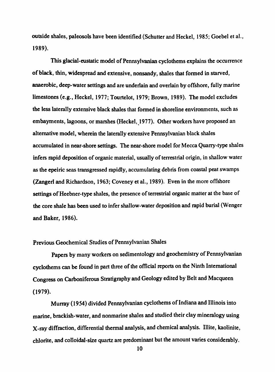
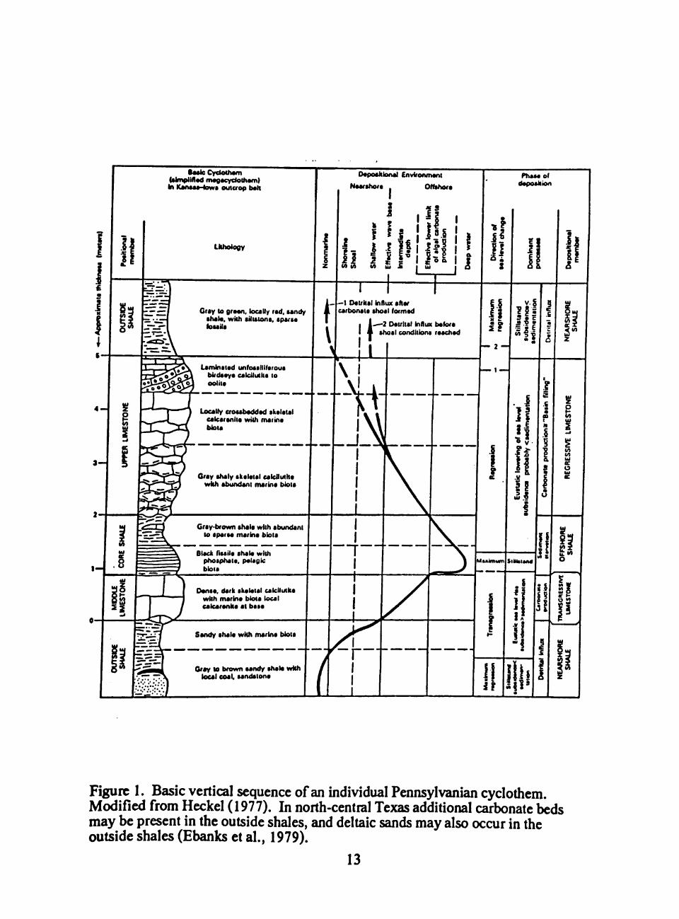
Figure 1. Basic vertical sequence of an individual Pennsylvanian cyclothem. Modified from Heckel (1977). In north-central Texas additional carbonate beds may be present in the outside shales, and deltaic sands may also occur in the outside shales (Ebanks et al., 1979).
13
A. Low Sea-level Stand (only small wind-driven vertical cells) WEST EAST
Open Ocean
Approx. depth (m) ^
0 =-
Position of periodic upwelling
Epicontinental Sea (HOOOs km in extent)
prevailing wind
7 TtMrmocliM ..... *v ,
2 0 0 - ^ '
carbonate + Iigtit-colored detritus
200 m
y^ tf" rir »'""<>"i V 2 i t v i i , I cf - \ j r PQ.-poor water Approximote
V^TpP* ^ position of i* V present Upper
y\4^ Pennsylvonlon jjF MId-Contlnent r^nami
^ (Konsos-Iowa) G«."?^°' , outcrop position of
B. High Sea-level Stand (large quosl-estuarlne cell) i upweiiing ««°, < < <- prevailing wind < < «
CoW.Ot-ooo^'*^* 200 —
blocK organic-rich fine detritus • phosp"^
< Prevailing winds
Oxygen-rich water
y Oxygen-poor water
Anoxic water
ocean currents
100
200
— 300
— 400
I I settling material _ 500 m
Figure 2. Cross-section showing low stand of sea level during regression and high stand of sea level during transgression in west-facing tropical epicontinental sea (Heckel, 1977).
14
present "X ..•••' . ..i"' \ •* i
<^ A \ A /COLO...'<.NEBRASKA1 \ \ ' A A': I ': •* ': .•:' UIKIM ^ .
IO»^-V '-/{
a * a * * a * *
V ^ A A . A A \ / ,•'••• \ \ YK"'""- X ^
;fA.>,TEXAJXTA' ta •:'.A
On^_6u°
km 500 • Appalachian Mtns.
Figure 3. Upper Pennsylvanian paleogeography of the Midcontinent Region of the United States showing position of paleoequator and areas of orogenic belts (Heckel, 1980).
15
MAXIMUM TRANSGRESSION •20'
./•••••••• > ^ w P 3 ^ a ^/• / . j
: B L A C K ^ 5 ^ S H A L E :
^ rupw«lllng :
Onl'l'ou^
km 900 S \ / A A A A A A A A A M A A A A A A A A A / ^
•• ••' / Appolachian Mtns. • v. / ,-• DLL I
Figure 4. Paleogeographic map showing probable facies relations of Upper Pennsylvanian Midcontinent sea during deposition of offshore shale along Midcontinent outcrop at phase of maximum transgression (Heckel, 1980).
16
20*
v LATE REGRESSION
<r . * • -
present A /• 1- I X
e»enL\ A - - A A/T-.--2>t/.:<>.Xpv'-'.i I \
}=rr'— ve_r —
;/«Poi,tf', \
TRADE
WIND
>r .A />^^ A>y:-.l- I i ' t , T - ^ T : " ^ J - ^ ' ' ' > ^ U ; - D :r f _o
r-. A^^:f.^,^Sio" ^LETAC^^.IT^^?y4^ \ i ^ - r r r BELT
/ "^AAAAnC" ./" t A v'l 'n.'i'^o''u° X*"
r t -•• • •• " A ' s C»» . . -
••ly
DOLDRUMS
I RAIN . ' , AA 0°
0 M 500
V'-'" '-i? K / D L L I
Figure 5. Paleogeographic map showing probable facies relations of Upper Pennsylvanian Midcontinent sea during deposition of upper part of regressive limestone, and locally base of nearshore shale along Midcontinent outcrop about midway through phase of late regression (Heckel, 1980).
17
CHAPTER n
LOCAL STRATIGRAPHY OF SECTIONS
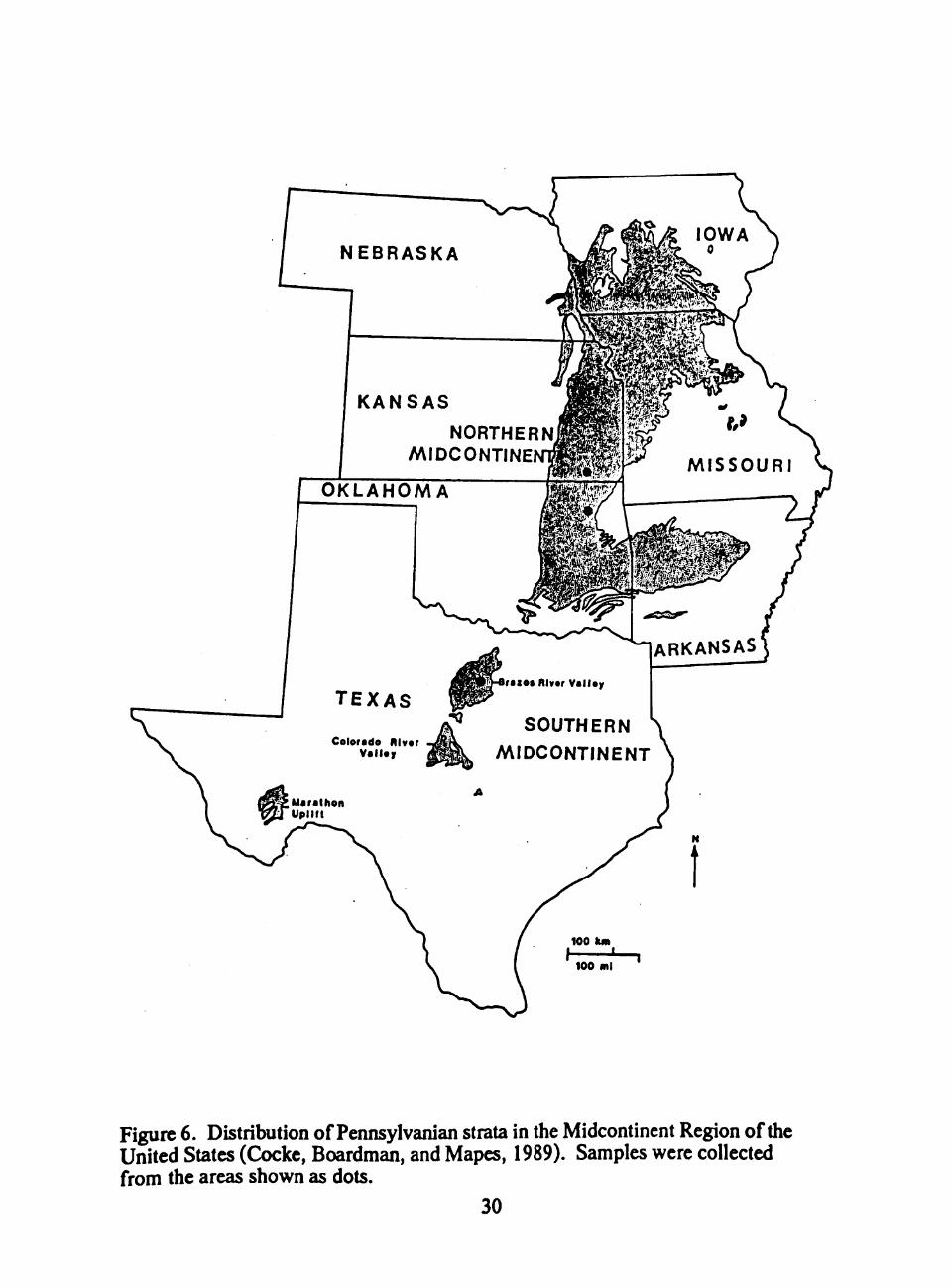
Shale samples were collected from the different geographic areas shown on the
map in Figure 6.
North-Central Texas
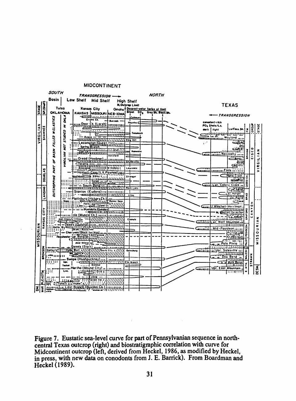
The majority of samples were collected from four cyclothemic intervals in north-
central Texas, that range in age from latest Desmoinesian to earliest Virgilian (Figure 7).
The intervals sampled were chosen because each is well-exposed in relatively fresh
roadcuts, permitting detailed sampling with little risk of sample contamination. The
stratigraphy and paleontology of the Middle and Upper Pennsylvanian cyclothems in
north-central Texas have been discussed in numerous works, the recent ones are those
by Boardman et al. (1989a, 1989b).
The pattem of deposition that characterizes Middle and Upper Pennsylvanian
cyclothems in north-central Texas (Boardman and Malinky, 1985) differs slightly from
the typical Kansas-type sequence. A plexus of terrestrial deposits containing freshwater
or terrestrial fossils and representing overbank deposits, marsh deposits, and paleosols
occurs at the base of the cycle. The terrestrial strata are directly overlain by a variety of
shallow marine deposits, the most typical of which may be either a greenish-gray
calcareous shale containing an open marine filter-feeding benthic association, or a thin
limestone, less than 0.3 m thick, bearing a fauna similar to that of the open marine shale.
Over these beds lie either a black, fissile phosphatic, organic-rich shale, a dark
gray-black, pyritic, bioturbated clay shale, or a medium to dark gray bioUirbated shale.
This lithofacies contains a sparse fauna dominated by pelagic organisms with essentially
no benthic elements. Ammonoids, conodonts, Dunbarella bivalves, and conularids 18
characterize the fauna of the black fissile shale lithofacies, which is fully developed in
only a few north-central Texas cycles. This association represents an anaerobic
environment apparently developed by the encroachment of the oxygen-minimum zone
from the nearby Midland Basin into the broad, gently sloping shelf area (Boardman and
Malinky, 1985; Brown, 1989)(Figure 8).
The dark gray-black clay shales, which directly overlie or may occur in place of
the black fissile shale lithofacies, contain a fauna dominated by ammonoids, conodonts,
nuculoid bivalves, and archaeogastropods. This association is dominated by detrinis
feeders, scavengers, and camivores and was designated by Boardman et al. (1984) as
the Sinuitina Conmiunity. Most skeletal remains are preserved by pyrite or limonite
after pyrite. The members of the Sinuitina Community are of small size, suggesting
mass mortality among junveniles along with possible stunting due to lowered oxygen
levels associated with a dysaerobic environment (Figure 8).
The dysaerobic interval characterized by the Sinuitina Conmiunity is overlain by
medium to dark gray shales that contain a fully aerobic community having the same
basic composition and trophic structure as the Sinuitina Community. However,
members of this association, the Treptospira Community of Boardman et al. (1984) are
full-sized, and preserved by calcite (Figure 8).
The black to dark gray shales described above correspond to the "core shale*' of
the Kansas cyclothem as interpreted by Heckel (1977). These are the maximum
trangressive deposits of the Texas cyclothems which accumulated in anaerobic and
dysaerobic environments, permitting preservation of organic matter in offshore clay
shales.
Above the Texas core shale interval any of a variety of lithofacies may occur
(Figure 9). The most common situation is where the core shale is overlain by a medium
to light gray shale containing a mixed marine association that is adapted to higher rates
19
of clastic influx. This shale is overlain by gray silty to sandy carbonaceous shale which
is ahnost devoid of marine benthic fossils, the prodeltaic facies. Higher in the section a
sequence of distal deltaic, proximal deltaic, and distributary channel facies, as described
by Erxleben (1975) is present. In areas lacking active deltaic progradation, the core
shale is directly overlain by a light gray to brown offshore open marine shale containing
a sequence of communities dominated by filter-feeding organisms. This open marine
shale may be overlain by a thick carbonate, the upper portion of which bears abundant
phylloid algae. The highest deposits include a variety of marginal marine shales that
grade into terrestrial deposits (Boardman and Malinky, 1985).
East Mountain Section
The East Mountain section (Figure 10) lies on the south side of East Mountain,
within the city of Mineral Wells, Texas (UTM GRID 14SNM58341363096). It is the
type locality of East Mountain Shale Member of the Mineral Wells Formation as
designated by Plummer and Moore (1922). Three transgressive-regressive cycles of
sedimentation occur in the East Mountain section (Merrill et al.,1987; Boardman et al.,
1989d). The lower two cycles are latest Desmoinesian in age, whereas the uppermost
one is earliest Missourian (Boardman et al., 1989d). The middle cycle containing the
East Mountain black shale bed was sampled for this study (EM section, Figure 10).
The uppermost part of the underlying cycle (UNIT 1) is gray to black coaly
shale that contains abundant plant compressions and one species of agglutinated
foraminifera. This unit has been interpreted to represent a marginal swamp
envirormient. A thin, positionally transgressive limestone (UNIT 2) forms the base of
the second cycle. The limestone is a sandy, limonitic wackestone to packstone and
bears an abundant marine fauna of ostracodes, microgastropods, and crinoid and
echinoid debris.
20
The core of the cycle is the East Mountain black shale bed which is a slightly
phosphatic fissile black shale (UNIT 3). The black shale contains the dysaerobic
benthic association of the 5iDu/tiha Community of Boardman and Malinky (1985) and
Kammer et al. (1986), which here also includes ammonoids, bivalves, and trilobites.
The black shale is characterized by abundant conodonts (>1000/kg at the base) of the
Gondolella-Idioprionodus biofacies, which has been interpreted to be a product of a
more offshore, dysaerobic environment by several workers (e.g., Heckel and
Baesemann, 1975; Heckel, 1977,1980, 1986; Boardman and Malinky, 1985; Yancey
and McLerran, 1988). An ahemate depositional model for Pennsylvanian black shales,
including the East Mountain black shale, has been presented by Merrill et al. (1987) and
Merrill and Grayson (1989). These workers place the dark gray to black shales into an
"organic-rich** marginal marsh envirormient where extremely high organic productivity
encouraged the abundant Gondolella-Idioprionodus biofacies to develop.
The succeeding dark gray shale (UNIT 4) contains the r/eptosp/'/a-Ammonoid
Community of Boardman et al. (1984) and a conodont fauna similar in species
composition to that of the black shale, but less diverse and abundant. This unit
accumulated in an offshore, slightly more oxygenated environment than the black shale
limestone of the Dog Bend at this section. The lower limestone (UNIT 2) is a massively
bedded fossiHferous packstone to grainstone that includes intraclasts and ooids among
its grains. It is interpreted to represent the basal transgressive unit of the cycle.
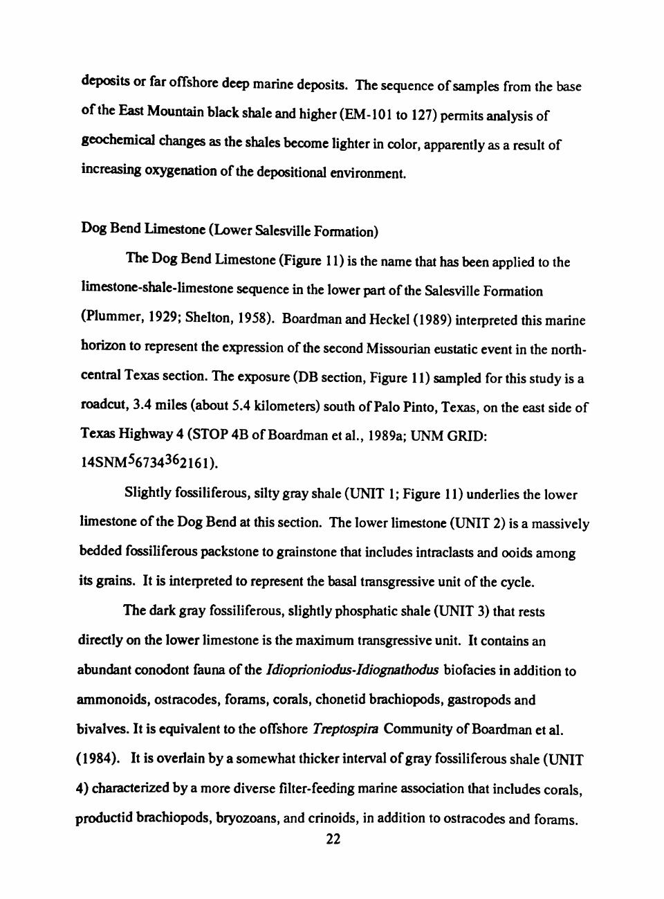
The dark gray fossiliferous, slightly phosphatic shale (UNIT 3) that rests
directly on the lower limestone is the maximum transgressive unit. It contains an
abundant conodont fauna of the Idioprioniodus-Idiognathodus biofacies in addition to
ammonoids, ostracodes, forams, corals, chonetid brachiopods, gastropods and
bivalves. It is equivalent to the offshore Treptospira Community of Boardman et al.
(1984). It is overlain by a somewhat thicker interval of gray fossiliferous shale (UNIT
4) characterized by a more diverse filter-feeding marine association that includes corals,
productid brachiopods, bryozoans, and crinoids, in addition to ostracodes and forams. 22
The upper limestone (UNIT 5) is a massively bedded wackestone to packstone, bearing
abundant corals and phylloid algae. It is overlain by highly fossiliferous marine gray
shale.
A series of samples were taken from the shale between the Umestones at this
section (DB-101 to 113) to analyze the elemental changes in a regressive shale sequence
that is bounded by carbonates and which was deposited in oxygenated environments.
Upper Salesville Black Shale
The upper Salesville black shale unit represents the expression of the third
Missourian marine eustatic event in north-central Texas (Boardman and Heckel, 1989).
Two sections of the upper Salesville black shale (3027 section. Figure 12; and UPS
section, Figure 13) were sampled in order to ascertain the nature and magnitude of
geochemical differences between nearby sections representing the same eustatic event.
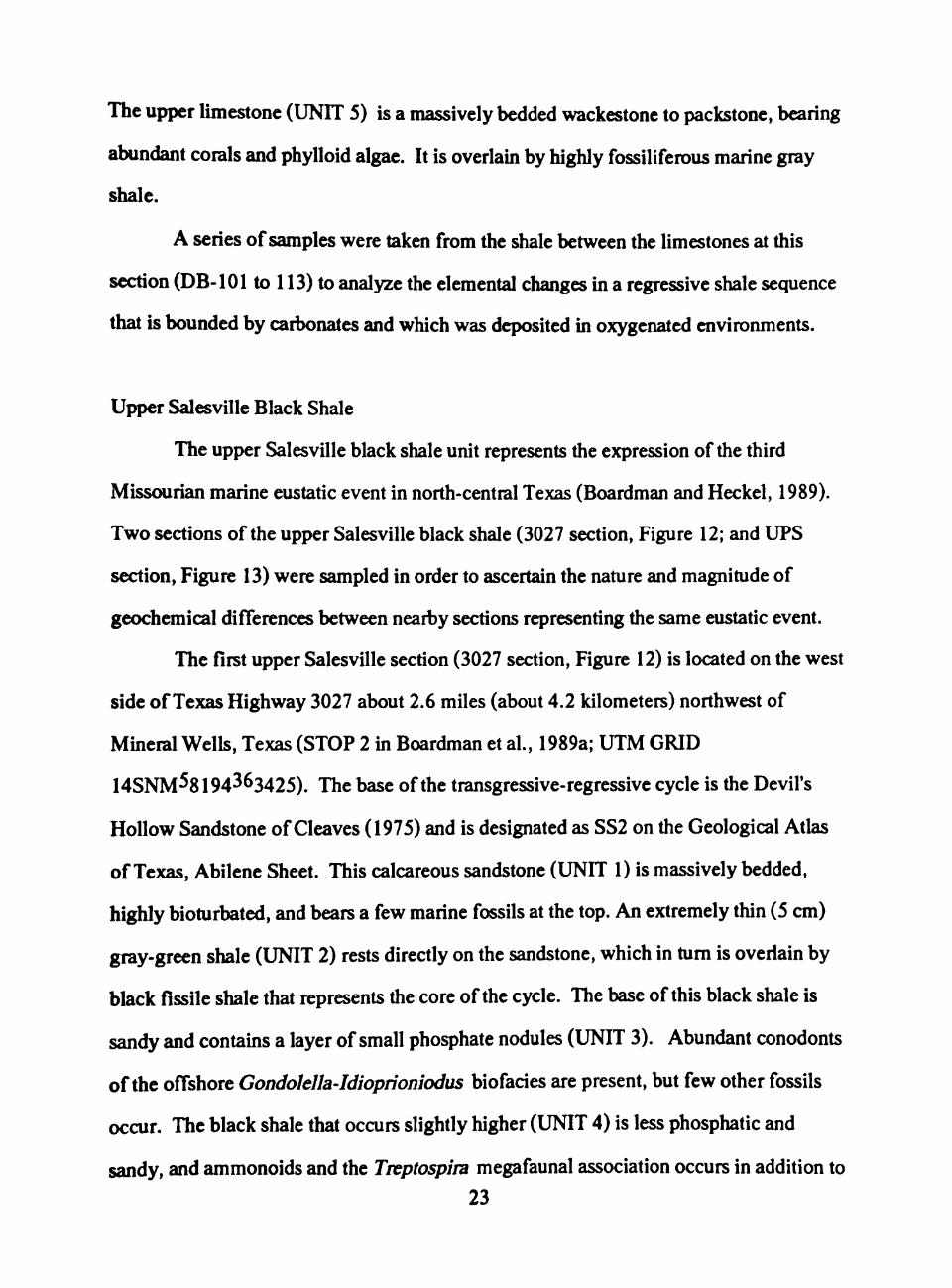
The first upper Salesville section (3027 section. Figure 12) is located on the west
side of Texas Highway 3027 about 2.6 miles (about 4.2 kilometers) northwest of
Mineral Wells, Texas (STOP 2 in Boardman et al., 1989a; UTM GRID
14SNM58194^63425). The base of the transgressive-regressive cycle is the Devil's
Hollow Sandstone of Cleaves (1975) and is designated as SS2 on the Geological Atlas
of Texas, Abilene Sheet. This calcareous sandstone (UNIT 1) is massively bedded,
highly bioturbated, and bears a few marine fossils at the top. An extremely thin (5 cm)
gray-green shale (UNIT 2) rests directly on the sandstone, which in turn is overlain by
black fissile shale that represents the core of the cycle. The base of this black shale is
sandy and contains a layer of small phosphate nodules (UNIT 3). Abundant conodonts
of the offshore Gondolella-Idioprioniodus biofacies are present, but few other fossils
occur. The black shale that occurs slightly higher (UNIT 4) is less phosphatic and
sandy, and ammonoids and the Treptospira megafaunal association occurs in addition to 23
conodonts of the Gondolella-Idioprioniodus biofacies. The black shale grades upward
into dark shale (UNIT 5), which contains a comparable megafaunal association, but less
abundant and diverse conodonts. The upper part of the section is a thick interval of gray
fossiliferous marine shale.
Samples were taken from the black shale interval above the Devil's Hollow
Sandstone, from the maximum transgressive anaerobic to dysaerobic core sh2ile into the
dysaerobic lithofacies. Evidence of chemical alteration attributed to weathering
(discoloration along fracttires) limited sampling to the lower part of the regressive shale
sequence.
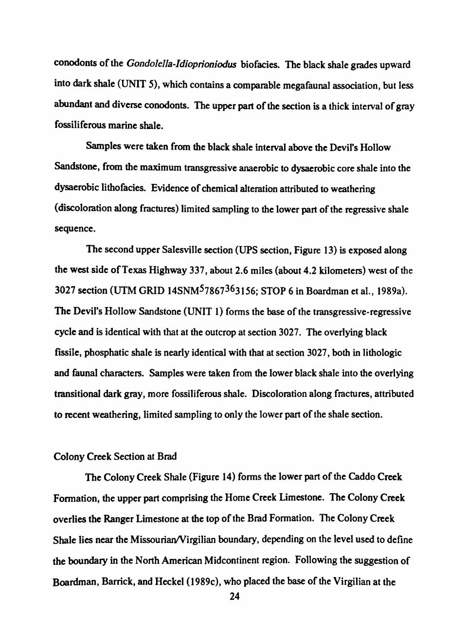
The second upper Salesville section (UPS section. Figure 13) is exposed along
the west side of Texas Highway 337, about 2.6 miles (about 4.2 kilometers) west of the
3027 section (UTM GRID 14SNM57867363156; STOP 6 in Boardman et al., 1989a).
The Devil's Hollow Sandstone (UNIT 1) forms the base of the transgressive-regressive
cycle and is identical with that at the outcrop at section 3027. The overlying black
fissile, phosphatic shale is nearly identical with that at section 3027, both in lithologic
and faunal characters. Samples were taken from the lower black shale into the overlying
transitional dark gray, more fossiliferous shale. Discoloration along fractures, attributed
to recent weathering, limited sampling to only the lower part of the shale section.
Colony Creek Section at Brad
The Colony Creek Shale (Figure 14) forms the lower part of the Caddo Creek
Formation, the upper part comprising the Home Creek Limestone. The Colony Creek
overlies the Ranger Limestone at the top of the Brad Formation. The Colony Creek
Shale lies near the MissourianA irgilian boundary, depending on the level used to define
the boundary in the North American Midcontinent region. Following the suggestion of
Boardman, Barrick, and Heckel (1989c), who placed the base of the Virgilian at the 24
Little Pawnee Shale in Kansas, the Colony Creek is considered to represent the
expression of the first major Virgilian eustaric event in north-central Texas. The section
(CCB section. Figure 14) along US Highway 180, west of Brad, Texas, was sampled
in this smdy (UTM 14SNM54362362305; STOP 13 of Boardman et al., 1989a). This
section was chosen not only for its excellent exposure, but also because of the study on
oxygen and carbon isotopes in shell material from this section published by Adlis et al.
(1988).
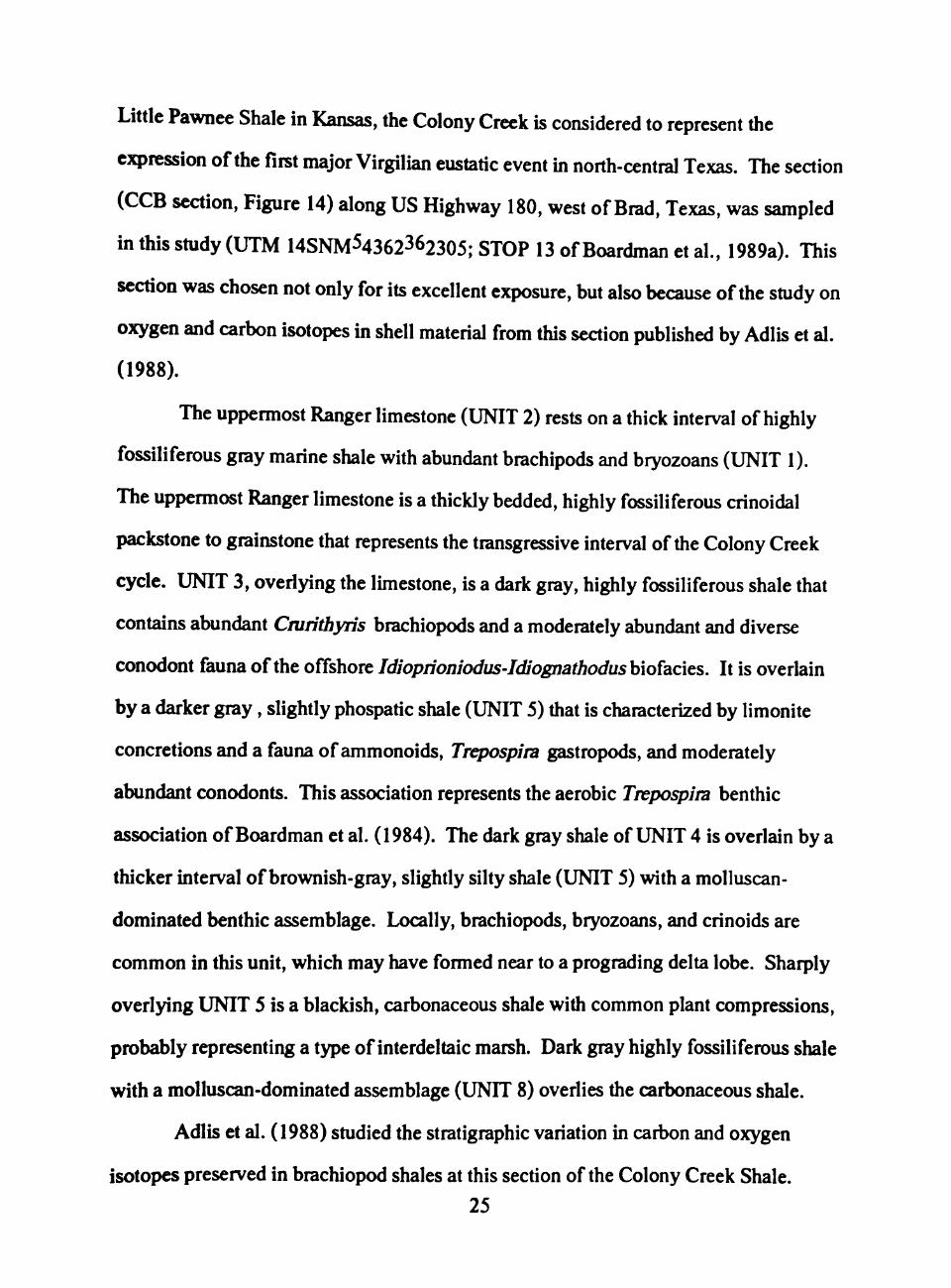
The uppermost Ranger limestone (UNIT 2) rests on a thick interval of highly
fossiliferous gray marine shale with abundant brachipods and bryozoans (UNIT 1).
The uppermost Ranger limestone is a thickly bedded, highly fossiliferous crinoidal
packstone to grainstone that represents the transgressive interval of the Colony Creek
cycle. UNIT 3, overlying the limestone, is a dark gray, highly fossiliferous shale that
contains abundant Cmrithyris brachiopods and a moderately abundant and diverse
conodont fauna of the offshore Idioprioniodus-Idiognathodushiofacies. It is overlain
by a darker gray, slightly phospatic shale (UNIT 5) that is characterized by limonite
concretions and a fauna of ammonoids, Trepospira gastropods, and moderately
abundant conodonts. This association represents the aerobic Trepospira benthic
association of Boardman et al. (1984). The dark gray shale of UNIT 4 is overlain by a
thicker interval of brownish-gray, slightly silty shale (UNIT 5) with a molluscan-
dominated benthic assemblage. Locally, brachiopods, bryozoans, and crinoids are
common in this unit, which may have formed near to a prograding delta lobe. Sharply
overlying UNIT 5 is a blackish, carbonaceous shale with common plant compressions,
probably representing a type of interdeltaic marsh. Dark gray highly fossiliferous shale
with a molluscan-dominated assemblage (UNIT 8) overlies the carbonaceous shale.
Adlis et al. (1988) studied the stratigraphic variation in carbon and oxygen
isotopes preserved in brachiopod shales at this section of the Colony Creek Shale.
25
These authors recorded a decrease in the delta ^^C values from 2.9-3.6 per thousand in
the lower 2 meters of the shale (Unit 3 and the lower part of UNIT 4) to 2.7-2.9 per
thousand in the 3 to 7 m interval (upper part of UNIT 4 into the middle of UNIT 5).
The delta ISQ values also show a shift from about -2.7 per thousand to about -3.0 per
thousand at the 3 meter mark. Although the shifts in delta l^o values were relatively
sli^t, Aldis et al. (1988) attributed the change to wanner water temperamres resulting
from a shallower water setting in the upper part of the section. By comparison with
modem analogues, an approximate maximum depth of 70 m was estimated for the core
of the cycle.
The Colony Creek section at Brad (CCB section, Figure 14) was sampled to
concentrate on three aspects. Detailed sampling at the base of the core shale section was
to determine elemental changes from maximum transgressive dysaerobic to areobic
settings. Samples in the interval of UNIT 3 through UNIT 5 parallel the isotopic
sampling of Aldis et al. (1988) to see if any elemental changes coincide with the isotope
stratigraphy. The blackish coaly shale of UNIT 6 was sampled to provide geochemical
information on organic-rich marsh deposits.
Kansas and Oklahoma
Two sections (LBK section. Figure 15; and TRR section. Figure 16) of
Permsylvanian shales in southeastern Kansas and northeastem Oklahoma were collected
to obtain samples from highly fissile, organic-rich, black shale typical of cyclothems in
the northern Midcontinent region.
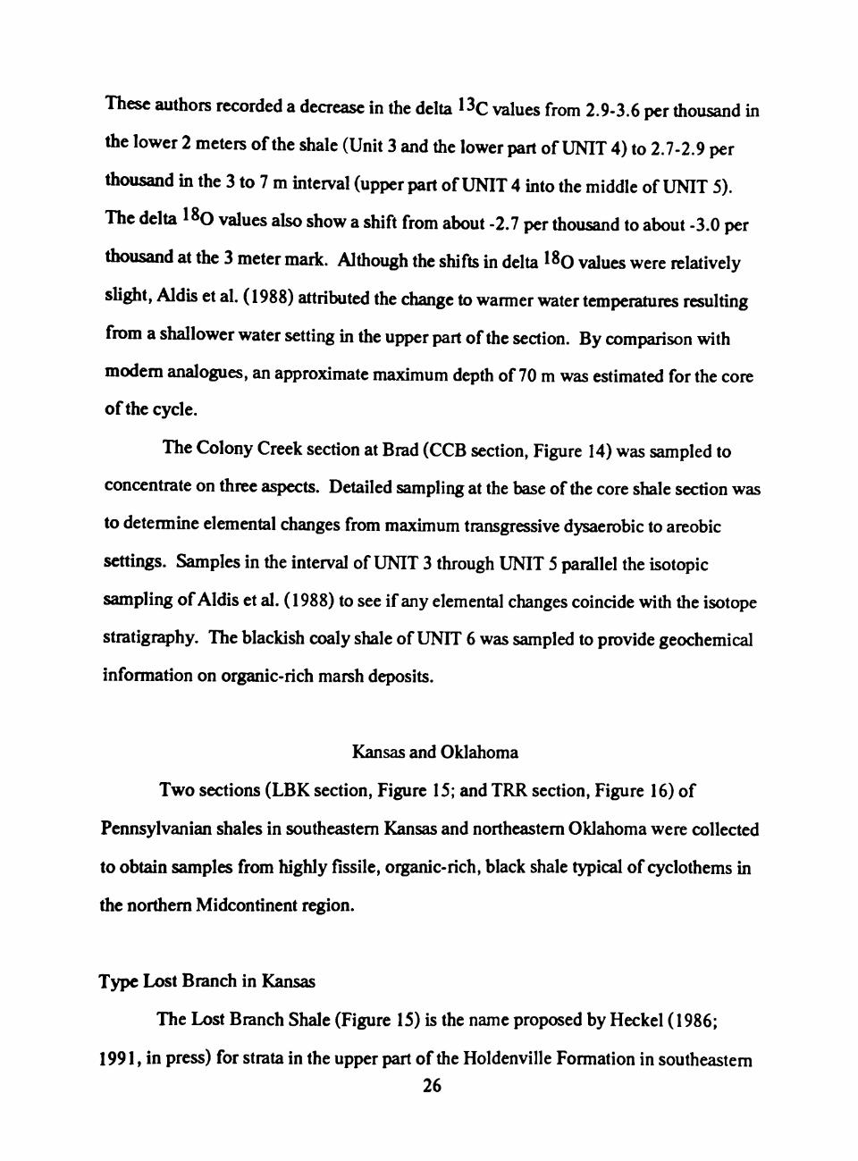
Type Lost Branch in Kansas
The Lost Branch Shale (Figure 15) is the name proposed by Heckel (1986;
1991, in press) for strata in the upper part of the Holdenville Formation in southeastem 26
Kansas and northeastem Oklahoma. The Lost Branch Shale overlies the Lenapah
Limestone and lies beneath the Hepler Sandstone, which forms the base of the
Missourian Pleasanton Group. At its type section along the Lost Branch of Pumpkin
Creek in southeastem Kansas ( NWl/4, sec. 10, T. 33 S., R. 18 E.), the Lost Branch
Shale includes the Dawson Coal (UNIT 1) and its underclay near the base. Fifteen
centimeters of dark gray shale (UNIT 2) bearing only a few invertebrate fossils overlie
the coal. The base oftheNuyaka Creek black shale bed (UNTT 3; Bennison, 1984)
rests with a knife-sharp contact on this gray shale. The Nuyaka Creek black shale
comprises 45 cm of black, highly fissile, conodont-rich, phosphatic shale that represents
the core shale of the highest Desmoinesian eustatic cycle. Nearly 4 m of gray shale with
abundant and diverse marine invertebrates (UNIT 4) rests with a sharp contact on the
Nuyaka Creek black shale. The Lost Branch Shale is interpreted to be equivalent to the
East Mountain black shale in north-central Texas (Boardman and Heckel, 1989).
The Nuyaka Creek black shale was sampled (LBK section. Figure 15) because it
is an excellent example of a highly fissile, organic-rich, black shale (Mecca Quarry-type
shale) that overlies a coal. The presence of sharp lithologic contacts at the base and top
of the black shale permits examination of the degree of mobility of elements out of black
shales into adjacent beds.
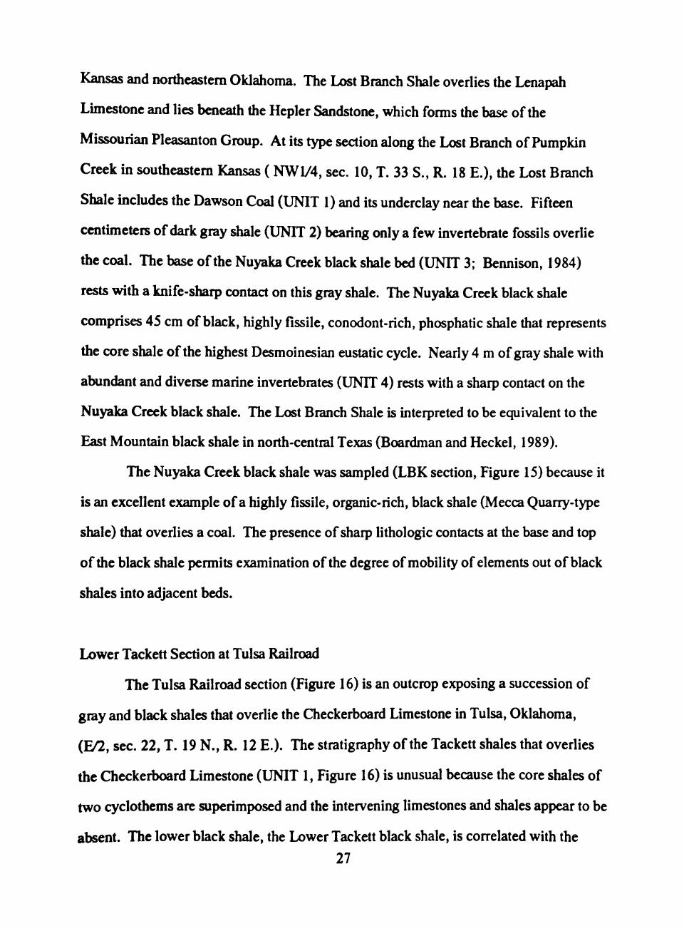
Lower Tackett Section at Tulsa Railroad
The Tulsa Railroad section (Figure 16) is an outcrop exposing a succession of
gray and black shales that overlie the Checkerboard Limestone in Tulsa, Oklahoma,
(E/2, sec. 22, T. 19 N., R. 12 E.). The stratigraphy of the Tackett shales that overlies
the Checkerboard Limestone (UNIT 1, Figure 16) is unusual because the core shales of
two cyclothems are superimposed and the intervening limestones and shales appear to be
absent. The lower black shale, the Lower Tackett black shale, is correlated with the
27
Mound City Shale in Kansas, and the upper black shale, the Upper Tackett black shale,
is correlated with Hushpuckney Shale of Kansas, the second and third Missourian
eustatic cycles according to Boardman and Heckel (1989). This atypical succession and
similar sections in the area of Tulsa may be due to the presence of a local basinal area
during the early Missourian, distant from sources of terrigenous elastics, which was not
completely exposed, even during low stands of sea level.
Although the Upper Tackett black shale is strongly weathered at the Tulsa
Railroad section (UNIT 6), the Lower Tackett black shale is freshly exposed and shows
litde sign of weathering. The blocky dark gray shale immediately below the Lower
Tackett black shale (UNIT 3) is apparently unfossiliferous and is separated from the
Checkerboard Limestone by a thin shale that may represent an underclay (UNIT 2). The
Lower Tackett black shale is a platy to fissile black shale that contains no calcareous
fossils and is phosphatic in only the upper 30 cm. It rests with a sharp contact on the
gray shale of UNIT 3, and is overlain, perhaps unconformably, by a thin interval of
calcareous gray shale (UNIT 5).
Like the Nuyaka Creek black shale, the Lower Tackett shale at this section was
sampled (TRR section, Figure 16) to determine the geochemical characteristics of a
highly organic, northern Midcontinent, black shale.
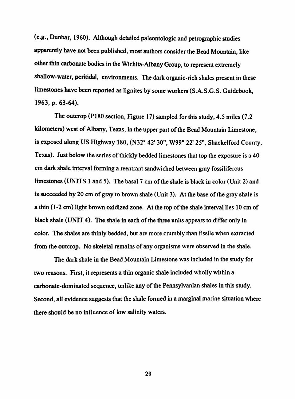
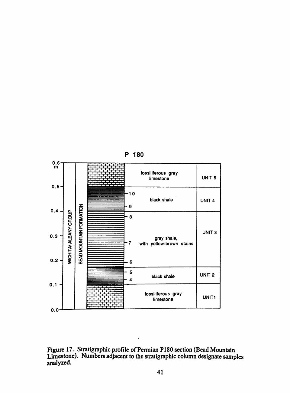
Permian Bead Mountain Limestone
A series of seven samples were taken from an organic-rich shale interval m a
section of the Lower Permian Bead Mountain Limestone west of Albany, Texas (PI 80
section. Figure 17). The Bead Mountain Limestone, part of the Wichita-Albany Group,
consists of a series of alternating limestone and marly shales that attain an average
thickness of 75 feet in Shackelford County and adjacent areas. It is shown to be early
Leonardian in age, as part of the Belle Plains Formation, on most correlation charts 28
(e.g., Dunbar, 1960). Although detailed paleontologic and petrographic studies
apparently have not been published, most authors consider the Bead Mountain, like
other thin carbonate bodies in the Wichita-Albany Group, to represent extremely
shallow-water, peritidal, environments. The dark organic-rich shales present in these
limestones have been reported as lignites by some workers (S.A.S.G.S. Guidebook,
1963, p. 63-64).
The outcrop (P180 section, Figure 17) sampled for this sttidy, 4.5 miles (7.2
kilometers) west of Albany, Texas, in the upper part of the Bead Mountain Limestone,
is exposed along US Highway 180, (N32*' 42' 30", W99'' 22' 25", Shackelford County,
Texas). Just below the series of thickly bedded limestones that top the exposure is a 40
cm dark shale interval forming a reentrant sandwiched between gray fossiliferous
limestones (UNITS 1 and 5). The basal 7 cm of the shale is black in color (Unit 2) and
is succeeded by 20 cm of gray to brown shale (Unit 3). At the base of the gray shale is
a thin (1-2 cm) light brown oxidized zone. At the top of the shale interval lies 10 cm of
black shale (UNIT 4). The shale in each of the three units appears to differ only in
color. The shales are thinly bedded, but are more cmmbly than fissile when extracted
from the outcrop. No skeletal remains of any organisms were observed in the shale.
The dark shale in the Bead Mountain Limestone was included in the smdy for
two reasons. First, it represents a thin organic shale included wholly within a
carbonate-dominated sequence, unlike any of the Pennsylvanian shales in this smdy.
Second, all evidence suggests that the shale formed in a marginal marine situation where
there should be no influence of low salinity waters.
29
Figure 6. Distribution of Pennsylvanian strata in the Midcontinent Region of the United States (Cocke, Boardman, and Mapes, 1989). Samples were collected from the areas shown as dots.
30
MIDCONTINENT SOUTH
TRANSGRESSION *• Bosin I Low Shelf Mid Shelf High Shelf
ROulcrep Limit
NORTH
D«tPttl-i»ol>f toeUt ol llmll TEXAS
TRANSGRESSION
•toMM-• HI*
- j m a - ' t ' ^Smm^f^^yhrTrrfFrn
Figure 7. Eustatic sea-level curve for part of Pennsylvanian sequence in north-centrkl Texas outcrop (right) and biostratigraphic correlation with curve for Midcontinent outcrop (left, derived from Heckel, 1986, as modified by Heckel, in press, with new data on conodonts from J. E. Barrick). From Boardman and Heckel (1989).
31
bO
S
8-
s Si o
! - < C: ON O OO • ON
o_r
32
o
.O • -
33
EAST MOUNTAIN (EM)
4 m
3 -
2 -
1 -
0 m
O
a: O Li.
IS
iS
East Mountain black shale bed
127
- 125
-123
-121
- 1 1 9
-117
gray shale
dark gray shale
113
109
105 103 101
black to dark gray fissile shale;
slightly phosphatic
y fossil, wackestone i B B B B B B B a B B B B B a a a a
99 98 97 96 95
gray clay shale with abundant plant detritus
UNITS
UNIT 4
UNIT 3
UNIT 2
UNIT1
Figure 10. Stratigraphic profile of East Mountain (EM) section. Numbers adjacent to the stratigraphic column designate samples analyzed.
34
DOG BEND LIMESTONE (DB) (LOWER SALESVILLE)
3 A m
2 -
1 -
0 m
fe cc O LJ-
UJ
UJ —I < CO
DOG BEND LIMESTONE
rs T * T
rri i±r
x^
I I £ ^
r ^
O i=z iS^ i S I I I o
I ' I ' ' r*T
r i - r i . X I ja
light gray shale
gray fossiliferous limestone
- 1 1 3
UNITS
UNITS
I . I . I ,
O O
O d III
cc
cx
111 gray shale,
with calcareous fossils
•109
• 107
-105 -103 .101
dark gray shale
light gray shale
UNIT 4
UNIT 3
UNIT 2
UNIT1
Figure 11. Stratigraphic profile of Dog Bend (DB) section (Lower Salesville). Numbers adjacent to the stratigraphic column designate samples analyzed.
35
3 m
2 -
1 -
0 m
Z o I-< a: O Li_ UJ
> CO UJ . J < CO
1 .
UPPER SALESVILLE SHALE (3027)
upper Salesville
black shale
dark gray shale
35
black shale
h 3 1
27
DEVIL'S HOtUDW
SANDSTONE
^—^^ 1 gray-green shale
••^••.•y.-:-:-:<-
23
UNITS
UNIT 4
19
15 phosphatic black shale
highly bioturbated sandstone
UNIT 3
UNIT 2
UNIT1
Figure 12. Stratigraphic profile of 3027 section (Upper Salesville). Numbers adjacent to the stratigraphic column designate samples analyzed.
36
UPPER SALESVILLE SHALE (UPS)
3 m
2 -
1 _
0 m
O fe CC
s UJ
UJ _ l < CO
upper Salesville
black shale
DEVIL'S HOLLOW
SANDSTONE • • • • • " • ' • • • " • • • • "
- 3 5
1-31
27
23
19
15
1 1
gray shale
dark gray shale with brown
alteration streaks
phosphatic black shale
highly bioturbated sandstone
UNIT 4
UNIT 3
UNIT 2
UNIT1
Figure 13. Stratigraphic profile ofUPS section (Upper Salesville). Numbers adjacent to the stratigraphic column designate samples analyzed.
37
COLONY CREEK SHALE (CCB)
12 m
1 0 -
8 -
6 -
4 -
0 m
fe CC
UJ UJ cc o 8 9 O
QQ
COLJONY CREEK SHALE
uppermost Ranger
J 27 *lark gray shale
-122 1-121
T25^26 ^T7T^124 black coaly shale
•119
•117
brownish-gray shale with marine
calcareous fossils
• 115
.113
•111
•109
•107 •105
gray-black shale slightly phosphatic
TT5T -102 .101
dark gray shale
gray packstone to wackestone
gray shale numerous calcareous
marine fossils
UNIT 7
UNITS
UNITS
UNIT 4
UNIT 3
UNIT 2
UNIT1
Figure 14. Stratigraphic profile of Colony Creek (CCB) section at Brad. Numbers adjacent to the stratigraphic column designate samples analyzed.
38
TYPE LOST BRANCH (LBK) KANSAS
Figure 15. Stratigraphic profile of Type Lost Branch (LBK) section in Kansas. Numbers adjacent to the stratigraphic column designate samples analyzed.
39
LOWER TACKETT SHALE (TRR) OKLAHOMA
4 m
3 -
2 -
1 m
UPPER TACKEFT BLACK SHALE
LOWER TACKETT BLACK SHALE
CHECKERBOARD LIMESTONE
black fissile shale
calcareous gray shale
39 37 3 5 33 29
.25
black fissile shale
gray shale
underclay?
fossiliferous gray limestone
UNITS
UNITS
UNIT 4
UNIT 3
UNIT 2
UNIT1
Figure 16. Stratigraphic profile of Lower Tackett Shale (TRR) at Tulsa Railroad Yard in Oklahoma. Numbers adjacent to the stratigraphic column designate samples analyzed.
40
P 180 0.6-m
0 .5 -
0.4 -
0.3 -
0.2 -
0.1 -
0.0-
cc O >-z
<
i o
cr
2 z
i IS CD
oc X^
T * T
X ^ J C
1
O
^
O S
r'=P X I X I
1.1 ,1
- 8
C: ^ ? S'
fossiliferous gray limestone
•10
9
black shale
gray shale, with yellow-brown stains
black shale
fossiliferous gray limestone
UNITS
UNIT 4
UNIT 3
UNIT 2
UNIT1
Figure 17. Stratigraphic profile of Permian PI 80 section (Bead Mountain Limestone). Numbers adjacent to the stratigraphic column designate samples analyzed.
41
CHAPTER m
GEOCHEMICAL ANALYSIS
Methods and Analysis
Sample Collection and Preparation
The rock samples were collected at intervals of less than 10 cm from fresh
outcrops. Plastic tools were used to separate the samples from the outcrop to avoid
metallic contamination. The collected samples were sealed in plastic bags for transport
to the laboratory. The rock samples were broken into smaller pieces using ceramic
mortar and pestle, and ground to about 200 mesh (75 micron) powder in a ceramic
shatter box. The powder form was used for chemical and X-ray analysis.
Mineralogy and Petrology
X-ray diffraction analysis of clay minerals was carried out with a Phillips
diffractometer using copper K-alpha radiation. The scanning speed and range were V
two theta per minute and 2°-65*', respectively. X-ray diffraction analysis showed that
quartz, kaolinite, and illite were present in all the samples; in addition, samples LBK-8,
10, 15, and TRR-25, 40 also contained pyrite. Amorphous substances were present in
the coal sample LBK-8. On the whole, there was insignificant variations in the relative
amounts of quartz, kaolinite, and illite in all the samples.
Thin sections of some of the rocks were made and examined under the
petrographic microscope. The shales are silty, some with quartz grains ranging from 10
to 30 microns, and others from 20 to 50 microns. Mica flakes are present in both gray
shales and black shales. The mica flakes are small, short, pieces, few in number, and
arc scattered. They are not observed in some samples probably because they are too
small and too widely disbursed. There are many dark brown aggregates of 42
clay + organics + oxides occurring as irregular spherical or elongated particles. These
aggregates of clay + organics + oxides are present in all the samples. They are most
likely composed of mixtures of illite + kaolinite, organic matter, and iron + manganese
oxides. Calcitic fossils occcur in most ofthe samples but vary in abundance. The
abundance of calcitic fossils varies inversely with the size ofthe silt fraction in the
samples. Grayish clay aggregates are made up of oval to spherical masses. These gray
aggregates are distributed irregularly. They are probably composed of kaolinite + illite
clay; kaolinite probably predominates because low birefringence was observed. Pyrite
is seen only in the black shale samples from sections TRR and LBK. Further details of
petrography are given in Appendix A.
Total Oiganic Carbon (TOC)
Various methods of total organic carbon (TOC) detennination are given by
Jeffrey and Hutchison (1981) and Johnson and Maxwell (1981). Comparisons of
methods to determine TOC are discussed by Leventhal and Shaw (1980). Three
different methods were used to measure TOC in this study.
Total oiganic carbon (TOC) can be determined by loss on ignition (LOI) at a
selected temperature. Details are given by Dean, 1974, (LOI at 550X); Ball, 1964,
(LOI at 375°C and at 850*'C); and Keeling, 1962, (LOI at 375°C). For this work, the
method of Dean (1974) was followed. Four grams ofthe sample were dried at 100°C
for one hour and the resulting weight loss was taken as the moisture content (Appendix
B). The samples dried at 100°C were subsequently heated at 550°C for one hour. The
loss on ignition at this temperature was converted to total organic carbon using Dean's
(1974) graph (Appendix B).
Gaudette et al. (1974) and Prince (1955) give details of wet combustion
measurement of TOC. For this work, the wet combustion method of Prince (1955) 43
was followed. The oiganic carbon in the sample was oxidized by acidified potassium
dichromate and the remaining unused dichromate was determined by back titration with
ferrous ammonium sulfate. The TOC was calculated from the amount of dichromate
needed to oxidize it (Appendix B).
Determination of organic carbon by infrared spectral analysis was done by Arco
Oil and Gas Company using a Leco carbon analyzer.
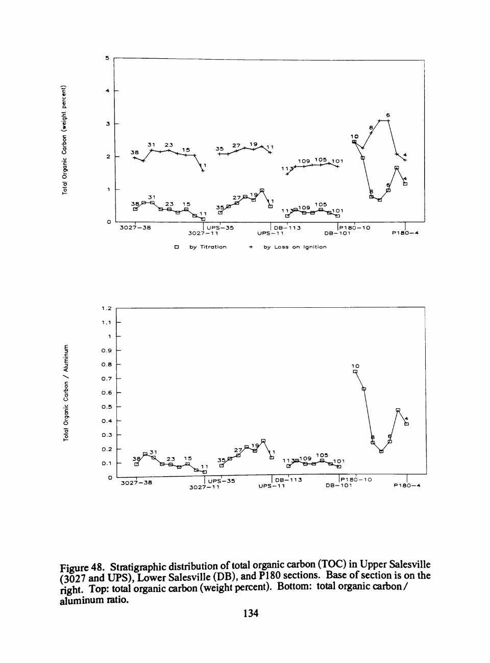
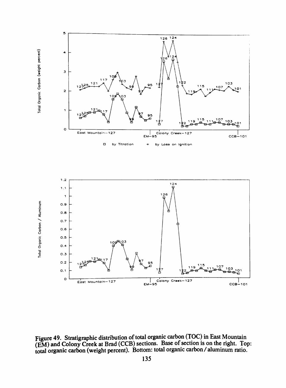
For the low organic carbon samples, TOC below 5 weight percent, the titration
method gives TOC values about 1.5 weight percent lower than that given by LOI
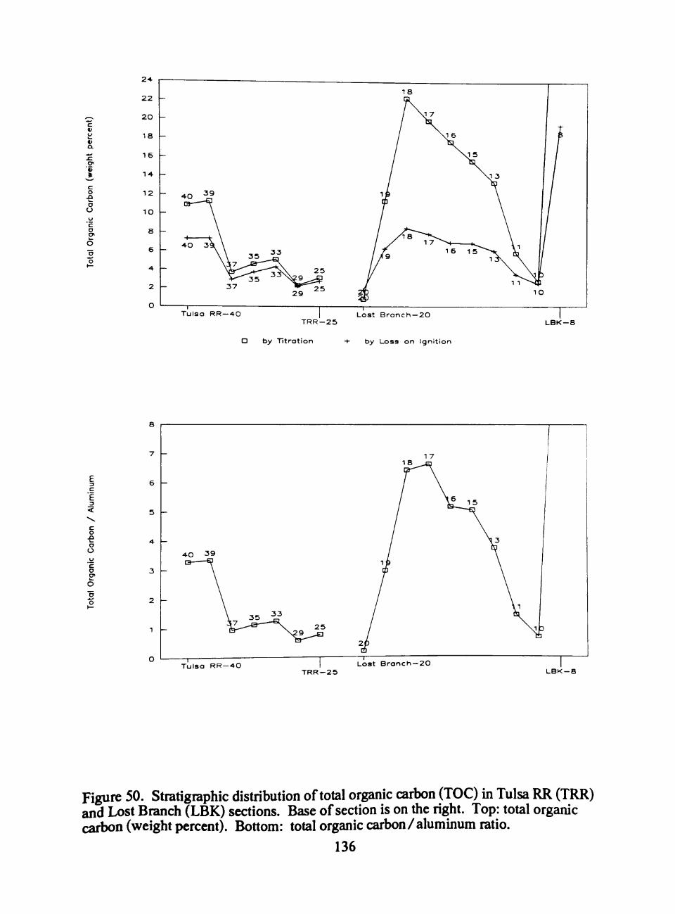
method (Figures 48 and 49 in Appendix C). For the high organic carbon samples, TOC
above 5 weight percent, the titration method gives higher TOC values than the LOI
method (Figure 50 in Appendix C). The higher the TOC, the larger is the difference in
TOC between the two methods. The TOC content variations are rcflected by both
methods for these low and high organic carbon shales. Only in samples from PI80
section do the titration and LOI methods yield a few TOC values that have opposite
trends, that is, TOC value is lower by the titration method but higher by the LOI
method.
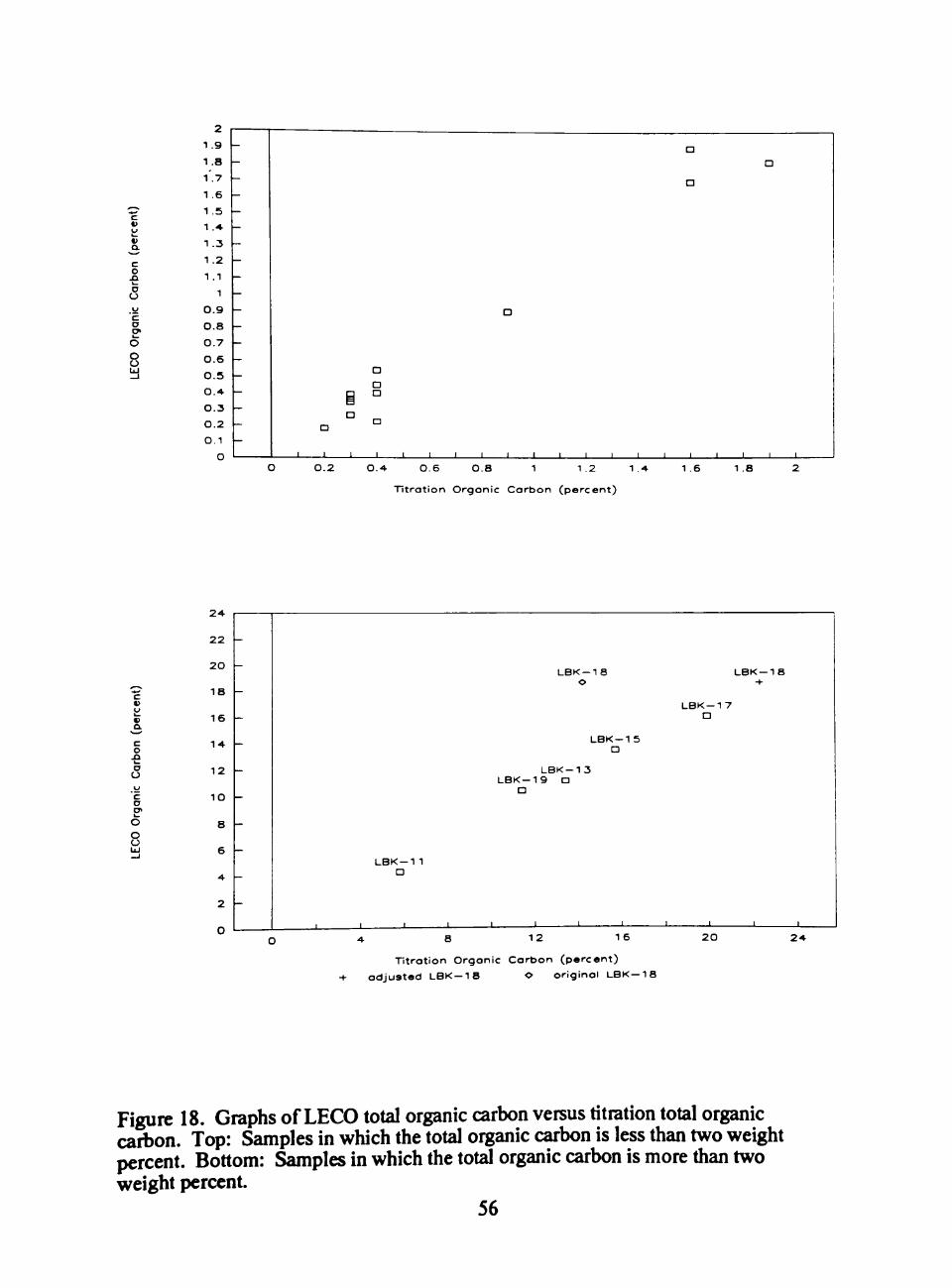
The LECO method gives TOC values comparable to those ofthe titration method
(Figure 18). For TOC values of less than 2 weight percent, the results ofthe two
methods differ by about 0.2 weight percent; for TOC values of more than 5 weight
percent, the difference is between 1 to 4 weight percent. The higher the TOC value, the
larger the difference. The values of TOC used to calculate TOC/Al ratios in this sttidy
are those obtained by titration. The TOC weight percent of LBK-18 obtained by titration
is unusually low comparcd to that obtained by LECO analysis. Consequently, the TOC
weight percent of LBK-18 was adjusted upward according to the value expected on the
basis of LECO analysis.
44
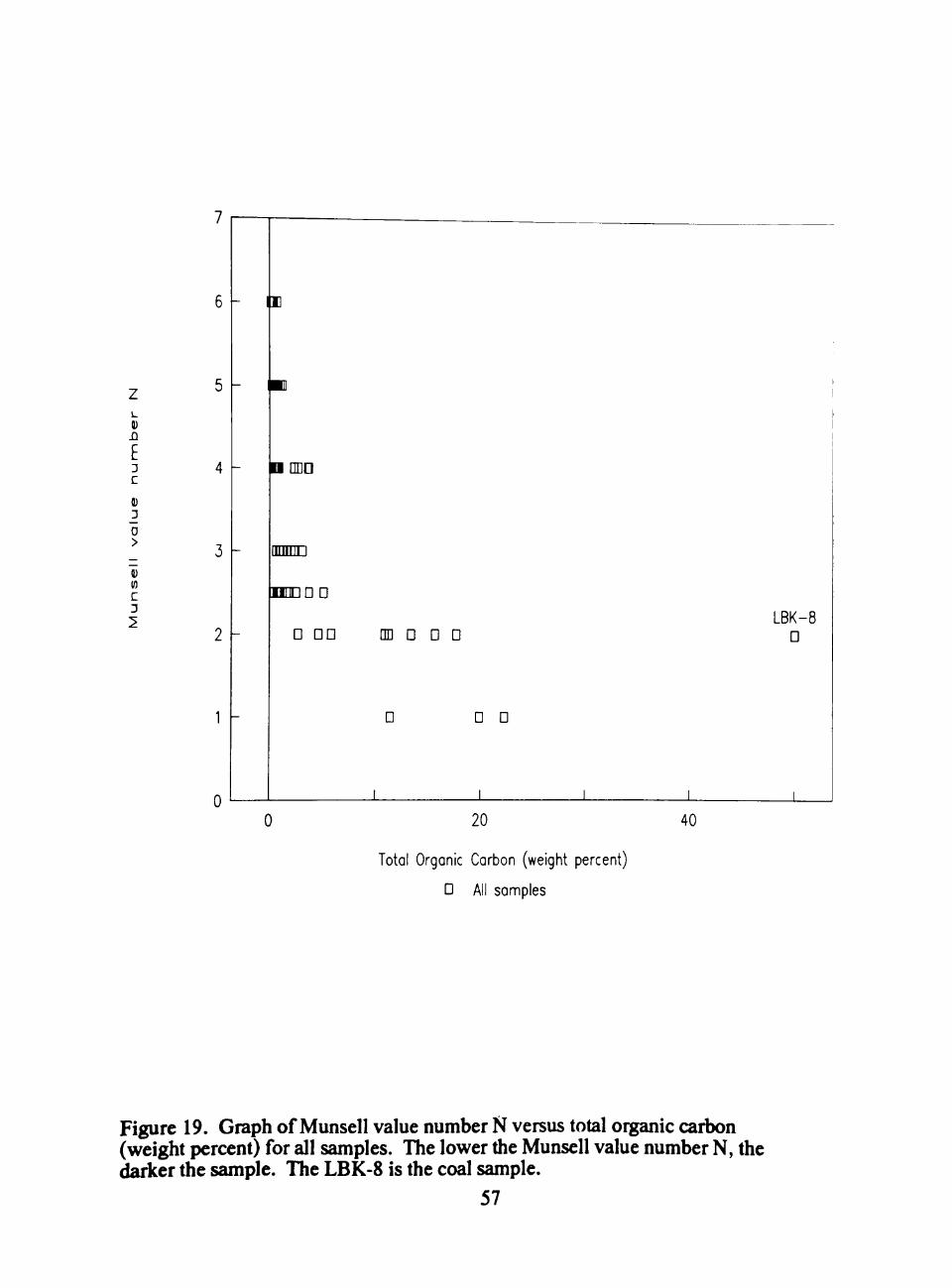
Color and Total Organic Caibon
Chroma, hue, and value are determined by comparing a fresh, dry whole rock
sample with the Munsell color chart (Appendix B). The graph of Munsell value number
N versus TOC weight percent is shown in Figure 19. The lower the value number N ,
the darker is the sample.
At low color value, the TOC varies widely. Therefore, one cannot visually
judge oiganic caibon content for black shales when the value number N is low. For the
gray shales in this smdy, the TOC varies within narrow limits and an estimation of TOC
can be made by visual inspection ofthe degree of blackness (the value number N). In
dark-colored marine shales, the degree of blackness maybe due more to the size and
distribution ofthe organic debris than to the actual concentration ofthe organic carbon
(Degens etal., 1957).
Discussions of color of shales are given by Myrow (1990); Blatt et al. (1980);
Potter et al. (1980); and Twenhofel (1939). The degree of blackness of gray to black
shales with TOC values below 5 weight percent is related to the TOC content according
to Potter et al. (1980) and Myrow (1990). However, the relationship is not strong
according to Blatt et al. (1980) due to the presence of dark-colored minerals like iron
sulfide, and the nature ofthe organic matter.
Ferrous Iron
Ferrous iron determination methods are given by Jeffrey and Hutchison (1981);
John and Maxwell (1981); Von Amd (1968); and Nicholls (1960). In this smdy, the
ferrous iron analysis was done according to the method of Von Amd (1968), The
ferrous ions in the sample were oxidized by acidified ammonium metavanadate ions and
the excess vanadate was determined by back titration with ferrous ammonium sulfate.
The concentration of ferrous ions was calculated from the amount of vanadate needed to 45
oxidize them to ferric ions (Appendix B). For shales with high TOC, the titration end-
point tends to be masked by the blackness ofthe suspension. The method of Nicholls
(1960) is able to overcome this difficulty by extracting the indicator into an organic
solvent. All titration methods use an oxidizing agent, and any sulfur compounds present
would also be oxidized giving higher ferrous iron values. An additional analytical
uncertainty is that the ferrous iron could be oxidized by the air during processing for
titration with resultant lower ferrous iron values. In Appendix B some parts in the
ferrous iron column were left blank because negative values were obtained when weight
percent FeO was subtracted from weight percent total iron (Fe203 + FeO). Most
probably, some organic carbon, in addition to any sulfur present, was oxidized by the
reagent giving false higher value of FeO.
Sulfur
Details of sulfur analysis are given by Canfield et al. (1986); Jeffrey and
Hutchison (1981); and Johnson and Maxwell (1981). Infrared spectral analysis for
sulfur was done for some ofthe samples in this study by Arco Gas and Oil Company
using a LECO sulfur analyzer.
Major and Trace Elements
Inductive coupled plasma (ICP) emission spectroscopy was used to determine
the abundance of selected elements. The ICP equipment used was Leeman model
plasma-spec 40. Rubidium was analyzed by Perkin-Ebner atomic absorption
spectroscope model 3030.
A 0.2 gram powdered sample was mixed with 1.2 grams of sodium metaborate
flux. The mixture was fused in a carbon crucible at 1000°C for 20 minutes. The molten
rock and flux were dissolved in 50 milliliters 5 percent HCl. The stirring time for 46
dissolution was 20 minutes. This solution was analyzed for trace elements. Twenty
milHliters ofthe original solution was mixed with 50 milliliters of 5 percent HCl and the
resulting dilution analyzed for major elements Results ofthe analyses are Hsted in
Appendix B. As the major elements of LBK-18 totalled above 150 percent probably due
to a dilution error, the major and minor element data of this sample were adjusted so that
the total percent ofthe major elements equal to the average ofthe total percent ofthe
major elements of LBK 13, 15, 16,17,and 19 (excluding LOI and H2O).
Presence of components other than the one being analyzed may affect the
analysis of the sample. Thisiscalledthematrixeffect (Hume, 1973). Sample CCB-
109 was used as an internal standard and given the code "BMS". The USGS internal
standards used were 1633A, SGR, and SCO (Seward, 1986; Johnson and Maxwell,
1981; and Flanagan, 1976).
Experimental uncertainty is calculated by dividing the sample standard deviation
ofthe intemal standard (BMS) by the mean and expressing it as a percentage. The
uncertainties for the data obtained by inductive coupled plasma spectroscopy are as
and yttrium. The Fe2V(Fe2++Fe3+) ratio of 0.9 for 3027-11 is the highest ofthe
Upper Salesville samples, being about twice the next highest.
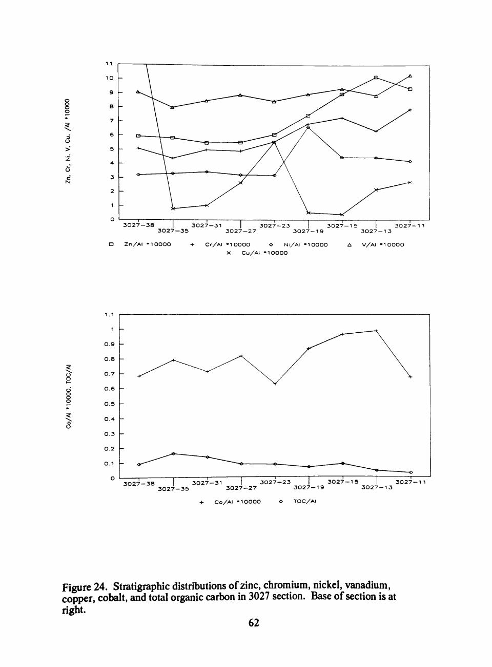
Zinc, chromium, cobalt, nickel, and iron (total) are more abundant in UNIT 3,
the lower black shale, than in UNIT 4 (Figure 24). The Fe2+/(Fe2++Fe3+) ratio rises
from about 0.2 in UNIT 3 to about 0.4 in UNIT 4.
50
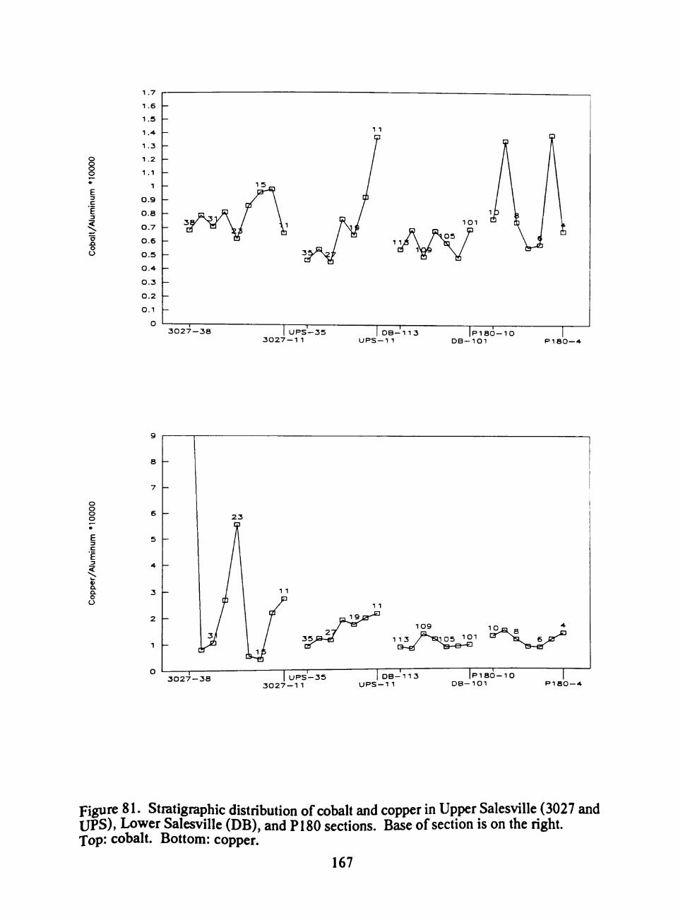
Copper shows a Cu/Al xlO^ ratio jump from 0.5 to 5.6 in going from sample
3027-19 at the top of UNIT 3 to sample 3027-23 in the base of UNIT 4. Copper also
has an extremely high abundance peak in the highest level sampled, 3027-38, near the
top of UNIT 4. No other elements show comparable variations at these stratigraphic
levels.
Calcium, magnesium, strontium, and manganese show a strong peak indicating
a maximum abundance at 3027-35, whereas phosphoms, and yttrium show a weaker
peak.
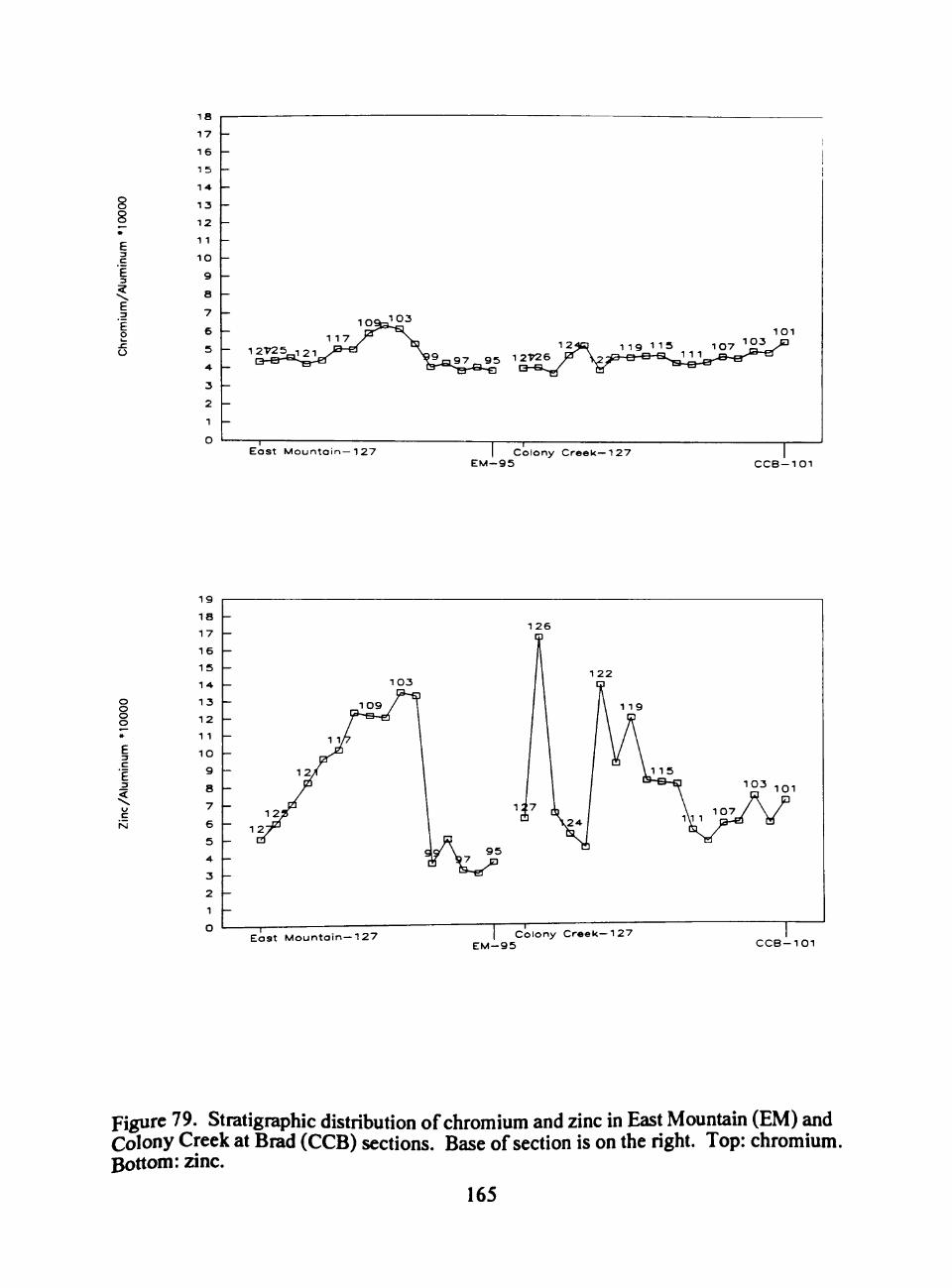
Colony Creek Section at Brad (CCB)
Total organic carbon is less than 0.5 weight percent in samples from UNITS 3,
4, 5, and 7. The black coaly shale of UNIT 6 contains between 2 and 4 weight percent
TOC. The TOC/Al ratio remains near a value of 0.05 through UNITS 3,4 and 5, and in
UNIT 6 it varies from 0.6 to 1.1. Ofthe five samples analyzed for sulfur from UNITS
3 and 4 (CCB-102 to 109), most contained around 0.03 weight percent sulfur, but
sample CCB-103 peaks at 0.14 weight percent.
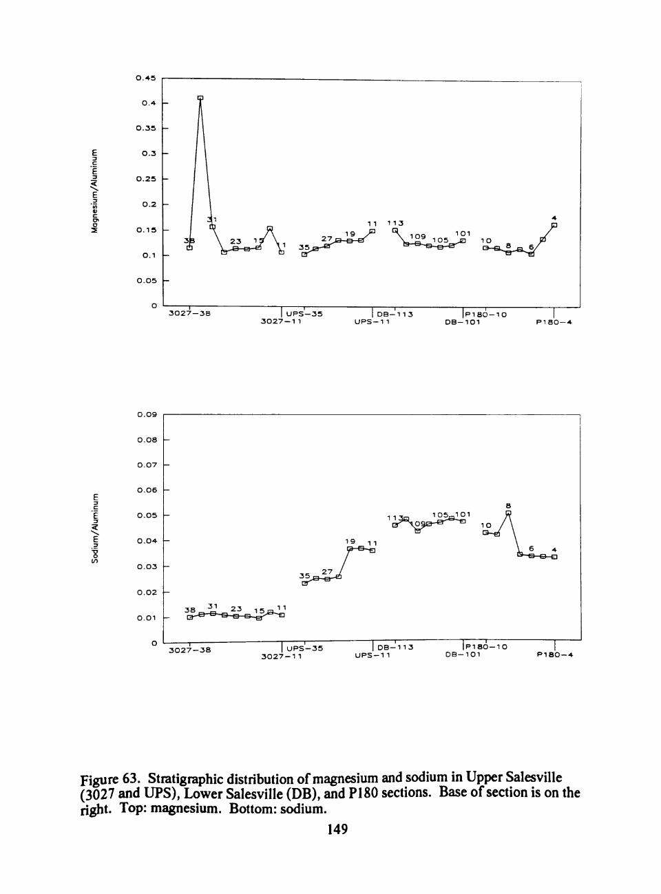
Silicon, titanium, zirconium, and sodium, and less so nickel, are more abundant
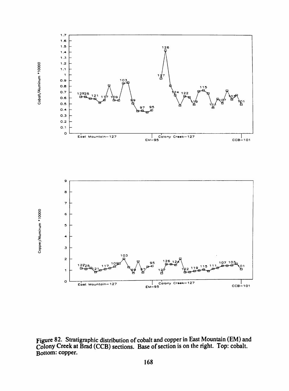
in the coaly shale of UNIT 6. Zinc, cobalt, beryllium, and yttrium show a peak at CCB-
126 at the top of UNIT 6, but otherwise show dissimilar distribution patterns for the rest
ofthe section. Potassium, mbidium, vanadium, iron (total), and magnesium show
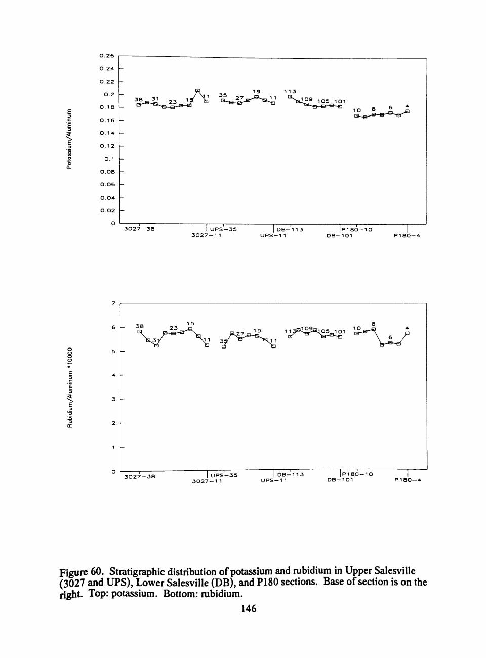
similar pattem, lower concentration in UNIT 6 than in the underiying shales.
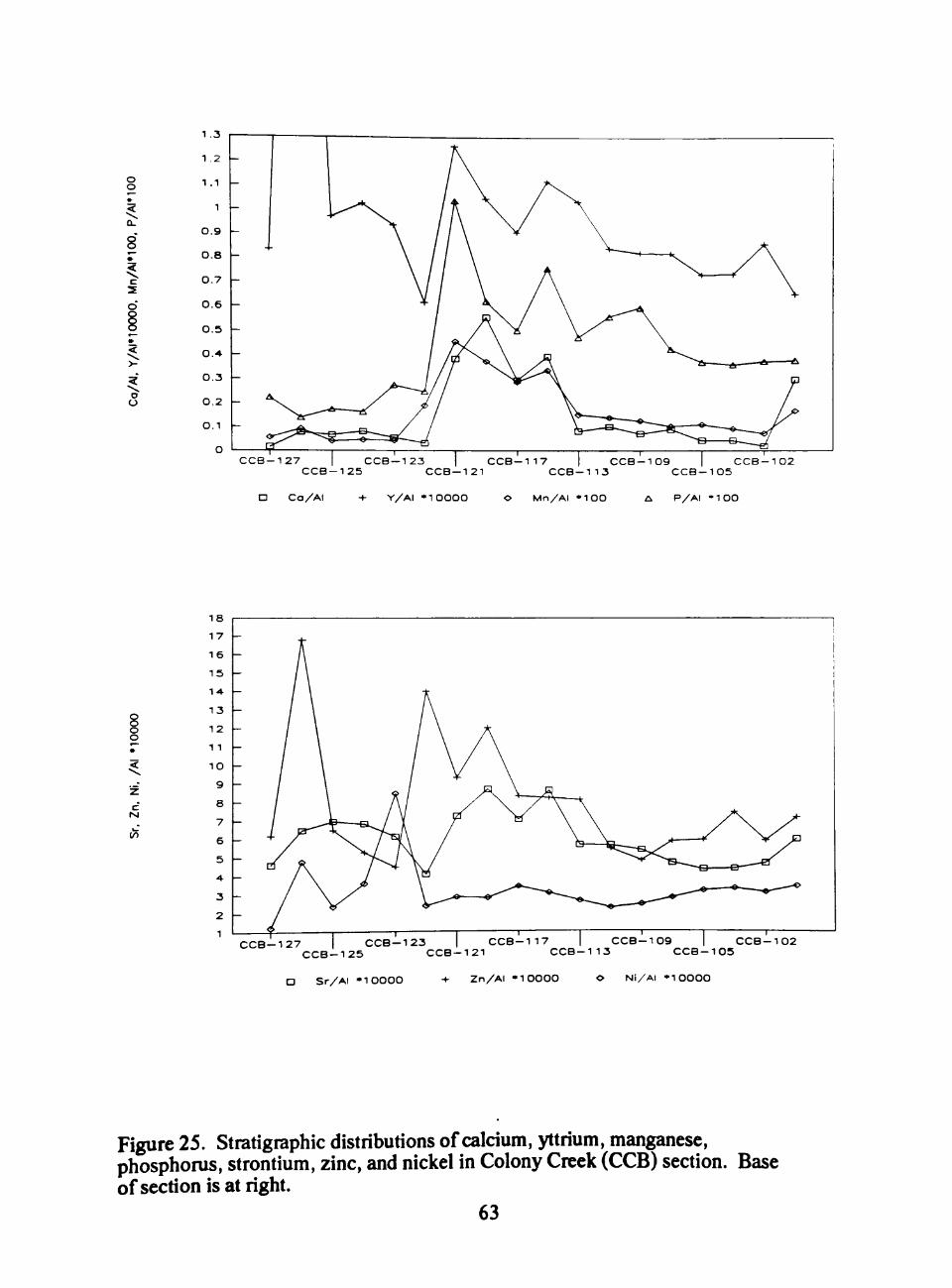
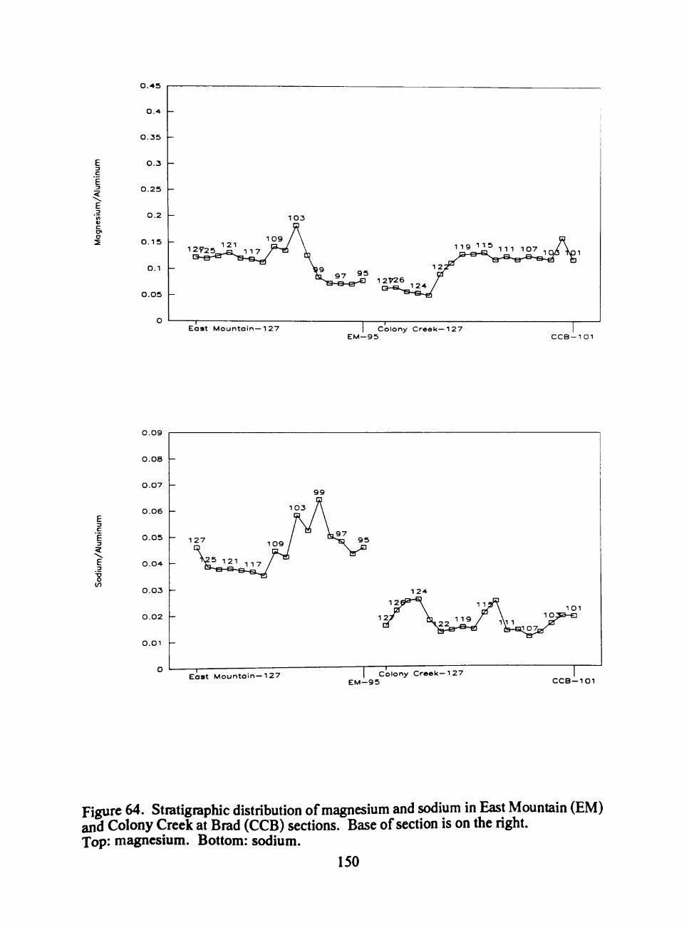
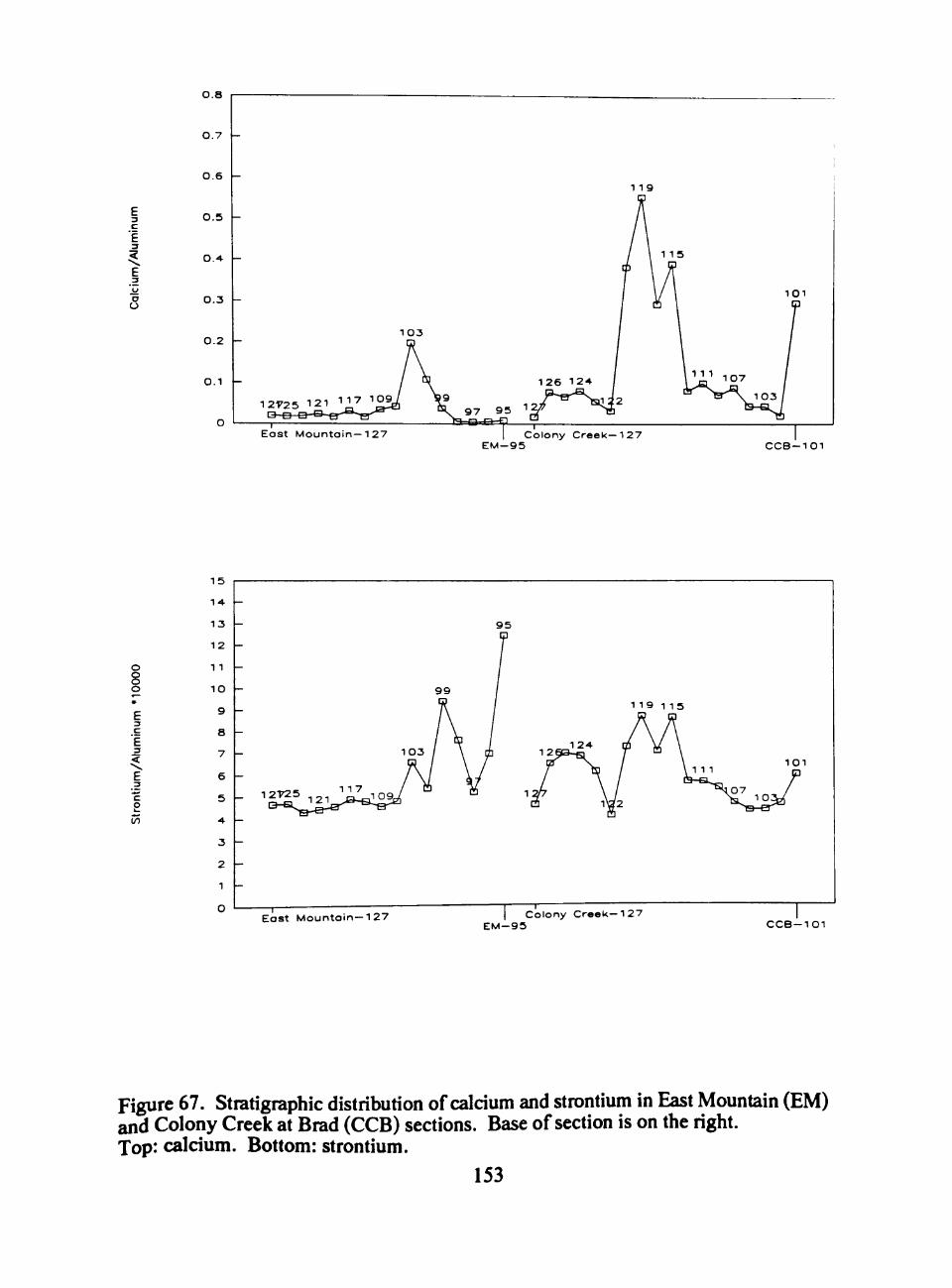
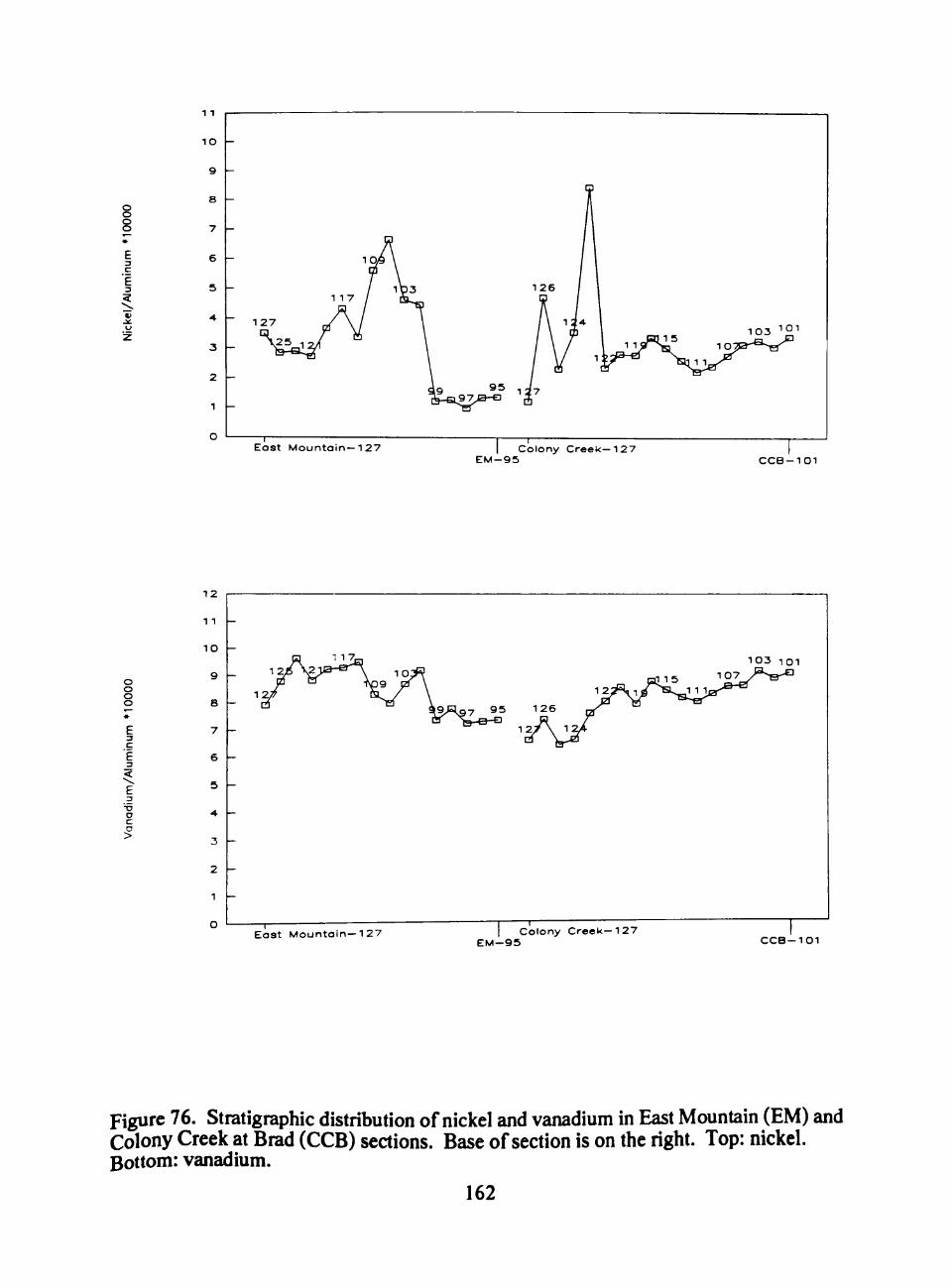
Unlike the black shale sequences at East Mountain and the two upper Salesville
sections, transition metals in Colony Creek shales do not show a pattem of high
abundance at the base and a decrease higher in the section. From UNIT 3 to UNIT 5
calcium, manganese, and strontium have a similar distribution pattem, that is, the
abundances are high at the base of UNIT 3, CCB-101, low through the rest of UNITS 3 51
and 4, and higher in UNIT 5 (Figure 25). In UNIT 6, these three elements fall to the
level of UNIT 4. Zinc also is somewhat more common in UNIT 5, than in other parts
ofthe section. At the base of UNIT 5 (CCB-113), sihcon, titanium, zirconium, and
sodium have a peak in abundance.
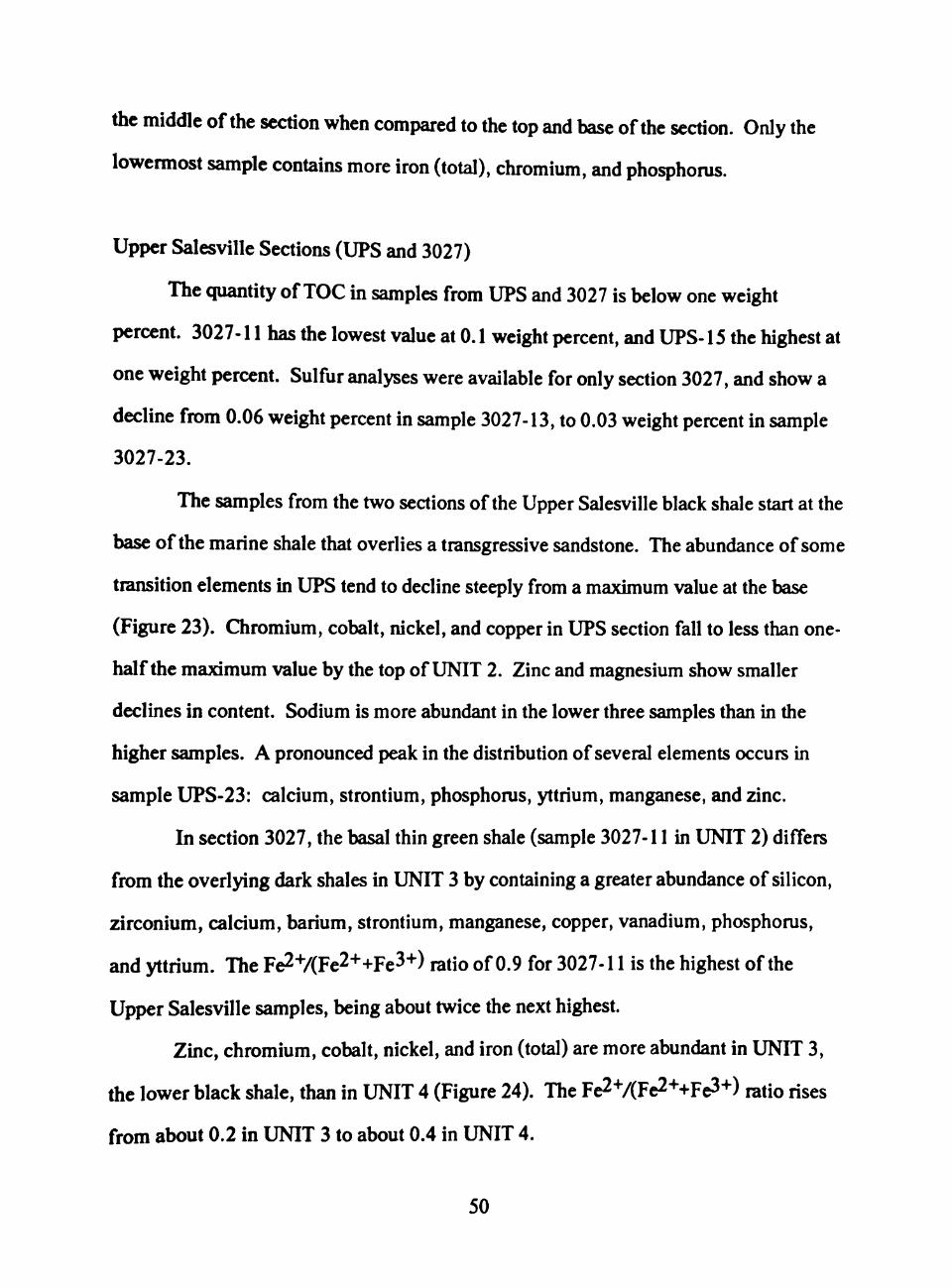
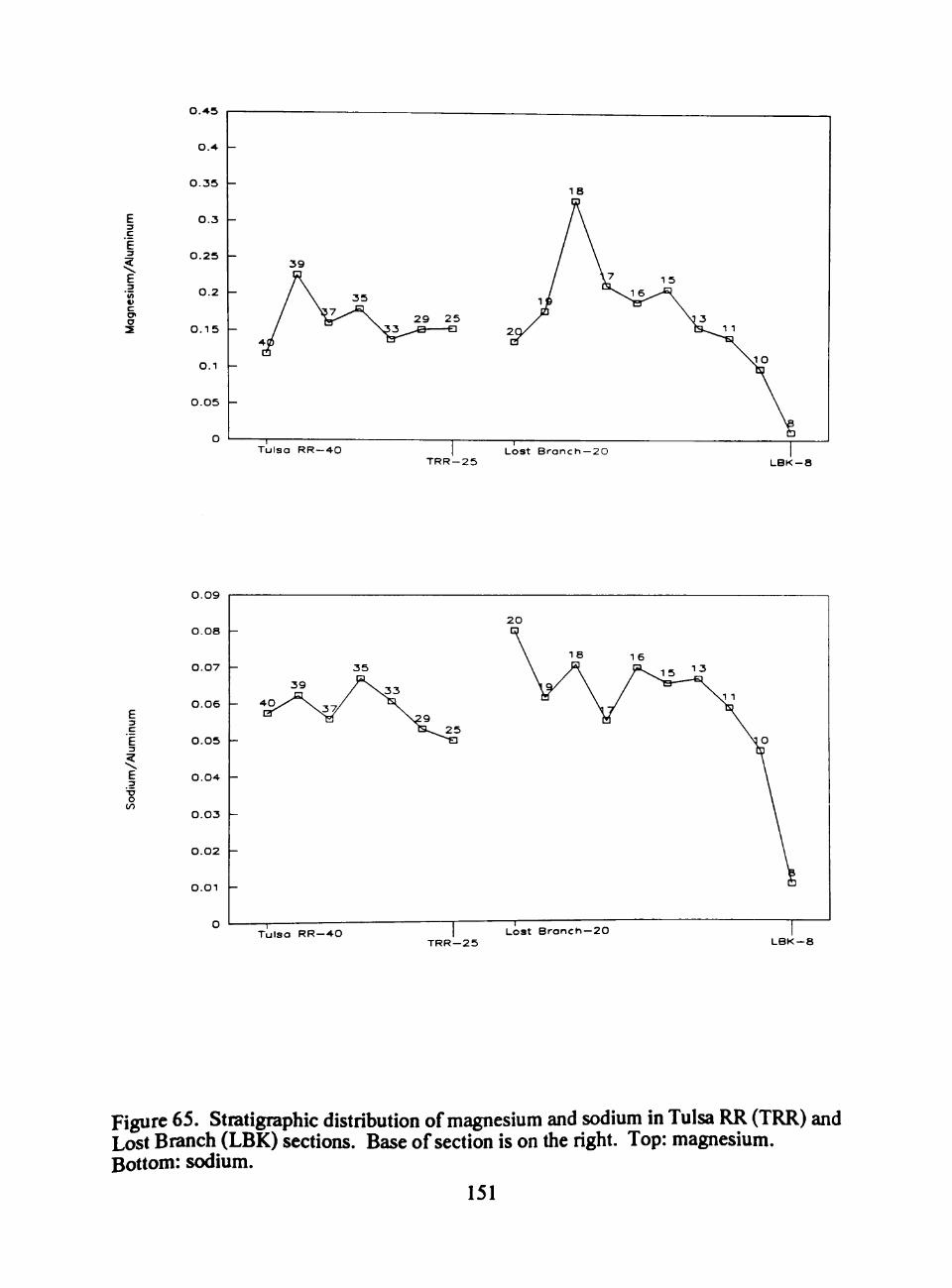
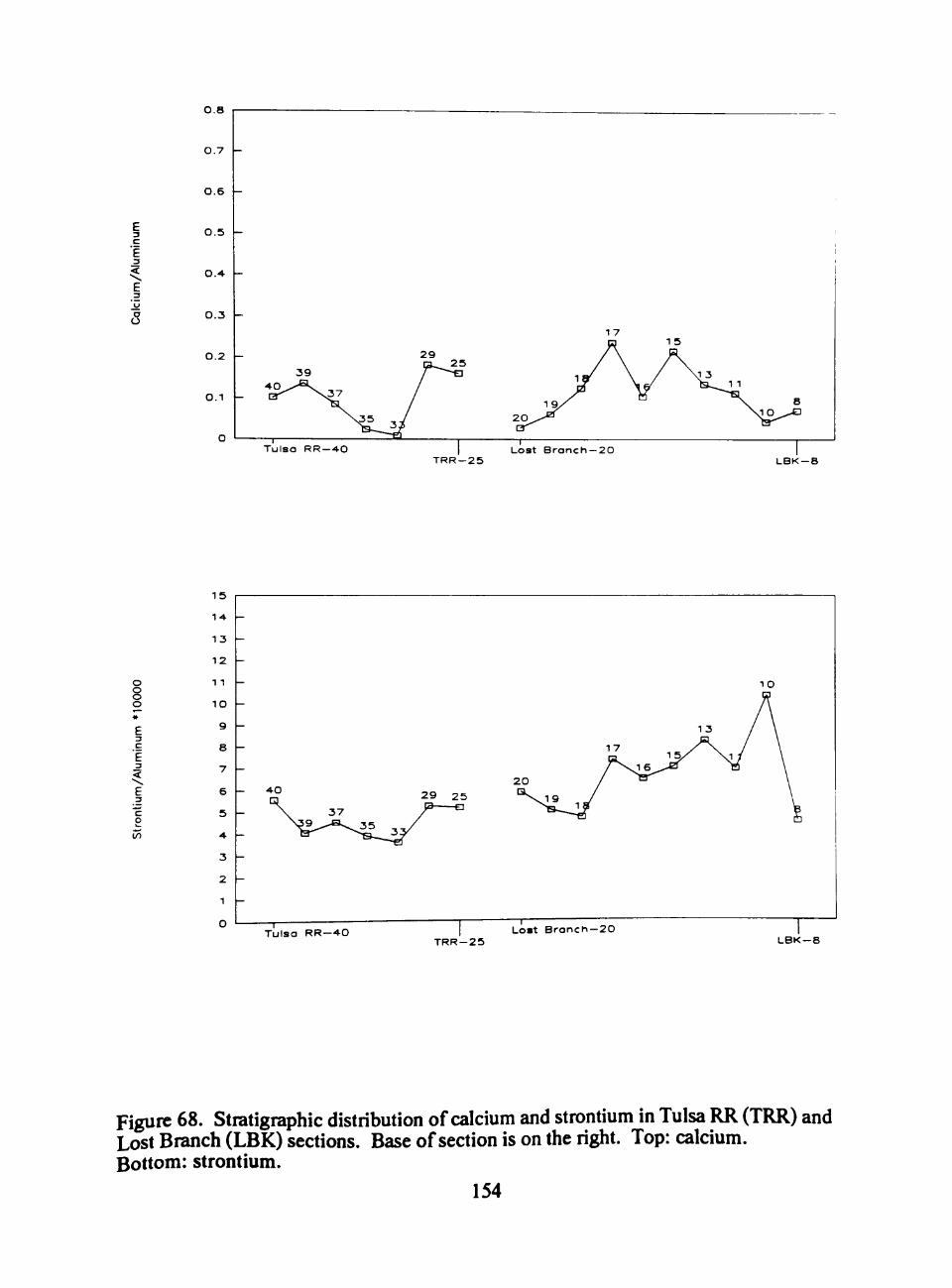
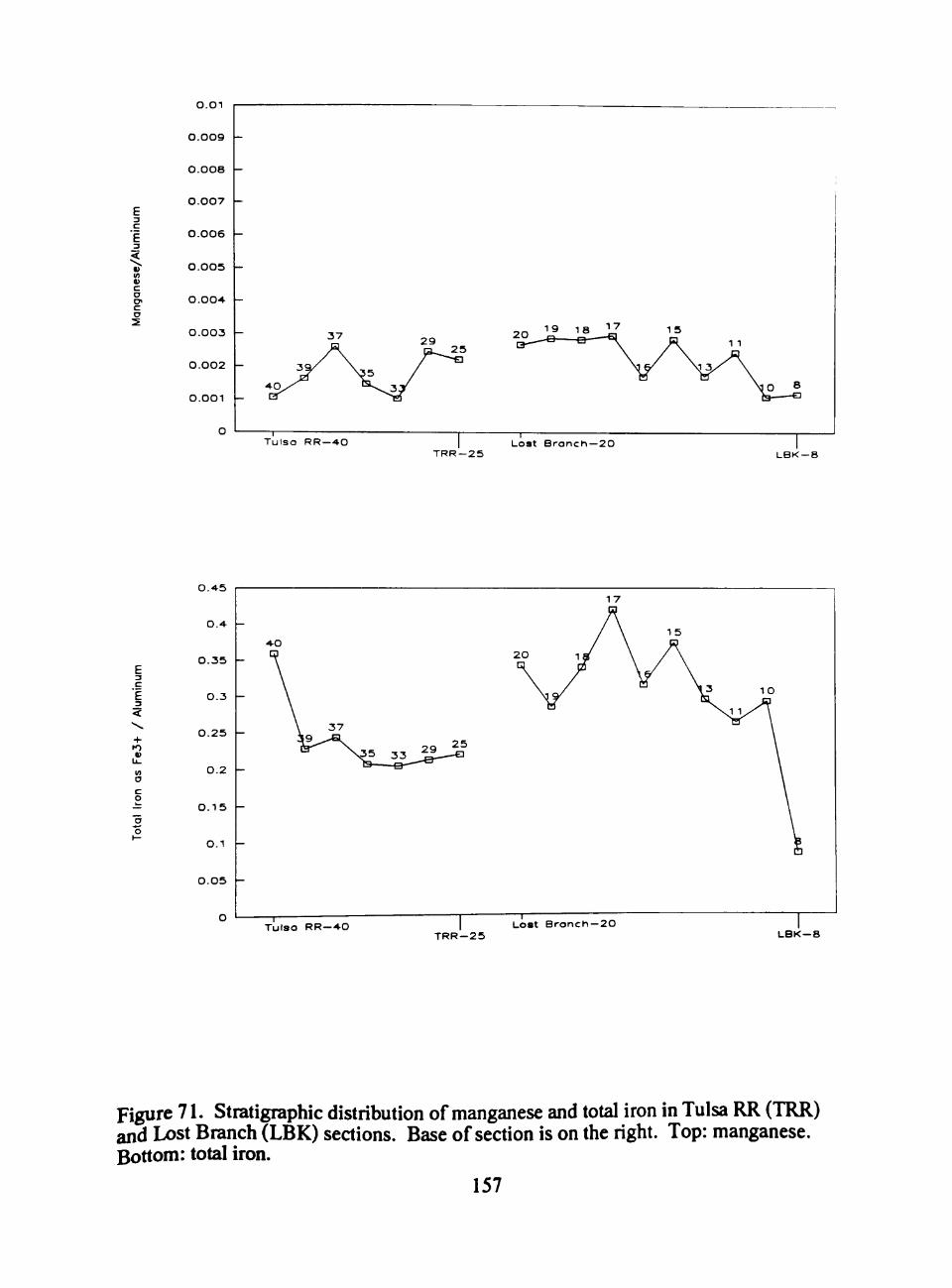
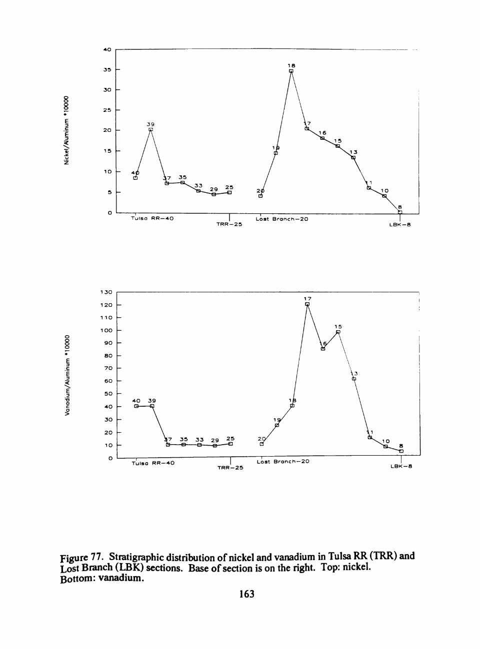
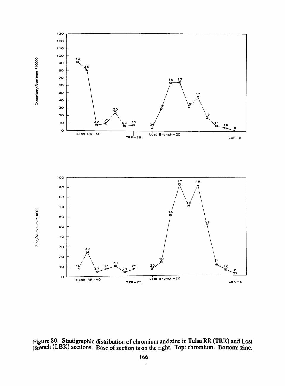
Type Lost Branch Section in Kansas (LBK)
The TOC in UNITS 2 and 4 are about 1 or 2 weight percent. From the base of
UNIT 3 (LBK-11) to the midddle (LBK-15 and 16), the TOC increases in abundance
from 5 to 19 weight percent, and then decreases from the middle of UNIT 3 to the top
(LBK-19) from 19 to 11 weight percent. Sulfur shows a similar increase and decrease,
with a maximum value of 4.3 weight percent in sample LBK-17 to lows of 2 weight
percent in sample LBK-11 at the base of UNIT 3, and 1 weight percent in sample LBK-
19, at the top of UNIT 3.
The S/Al ratio correlates positively with the TOOAl ratio and the trend of ratios
of LBK-13, 15, 17, and 19 passes through the x-axis at TOC/Al ratio of about 2 (Figure
26). The S/Al ratio correlates with the total Fe/Al ratio (Figure 26) and although the
correlation line ofthe two ratios does not pass through the origin it is parallel to the
stoichiometric FeS2 line. The stoichiometric FeS2 line is based on the theoretical ratio
in pyrite of two sulfur atoms to one iron atom.
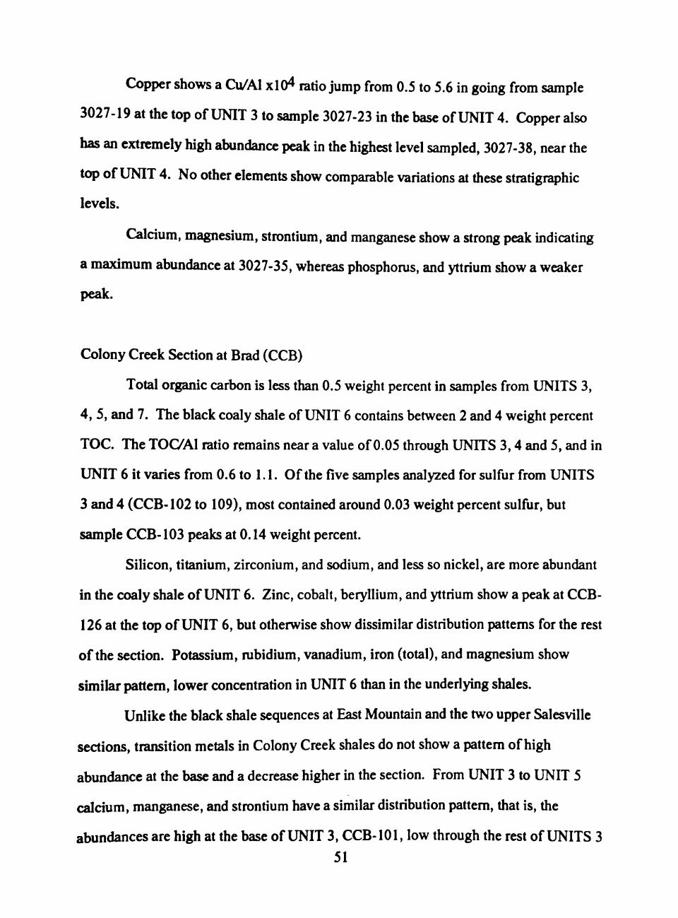
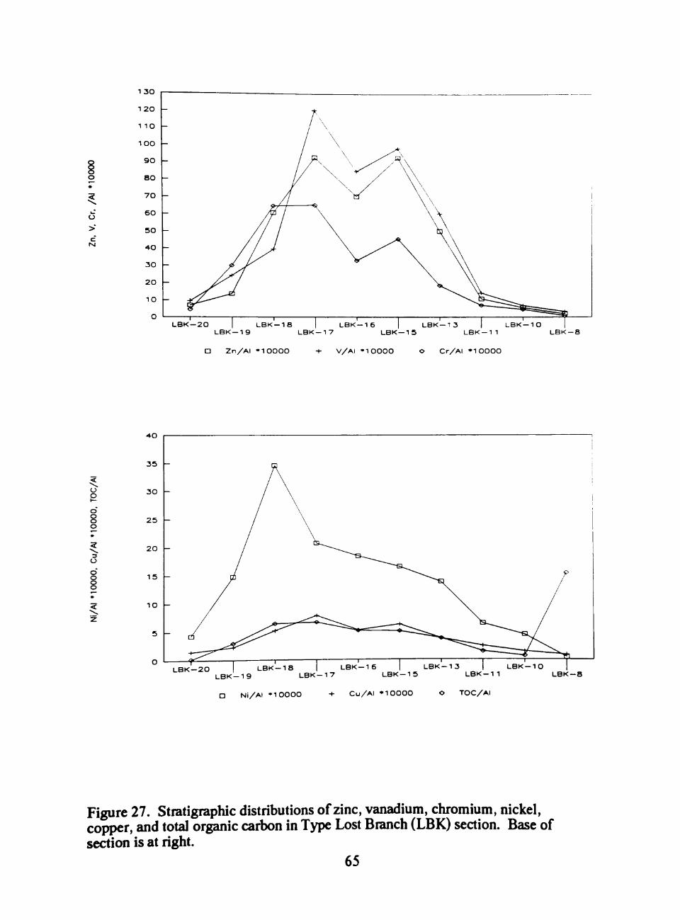
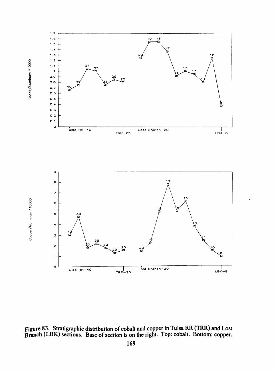
From the base of black fissile shale UNIT 3, several elements increase steeply at
LBK-13, attain their greatest abundance in the upper part of UNIT 3, but decline at the
top ofthe UNIT (Figure 27). All these elements are significantly less in the gray shales
of UNIT 2 below, and UNIT 4 above.
Vanadium, zinc, copper, and to a lesser degree calcium, have prominent
abundance maxima in samples LBK-15 and 17, separated by a lower content in sample
LBK-16. From the base of UNIT 3, vanadium has nearly a tenfold increase in the 52
V/Al xlO^ ratio to a maxiumum of 120 in LBK-17, and copper has a threefold increase
to a Cu/Al xlO^ ratio maximum near 8 in LBK-17. Zinc shows an ninefold increase to a
maximum Zn/Al xlO^ ratio of over 90 in LBK-15 and 17.
The contents of nickel and magnesium also rise sharply from the base of UNIT 3
(from sample LBK-11), and attain a maxunum value in LBK-18 but have no significant
peak in LBK-15 or 17. The distribution of chromium and cobalt show a weak peak at
LBK-15; chromium attains its greatest abundance in LBK-17 and 18, and cobalt in
LBK-18 and 19. Beryllium also shows a slight increase from the base of UNIT 3, with
maximum abundances in LBK-17 to 19.
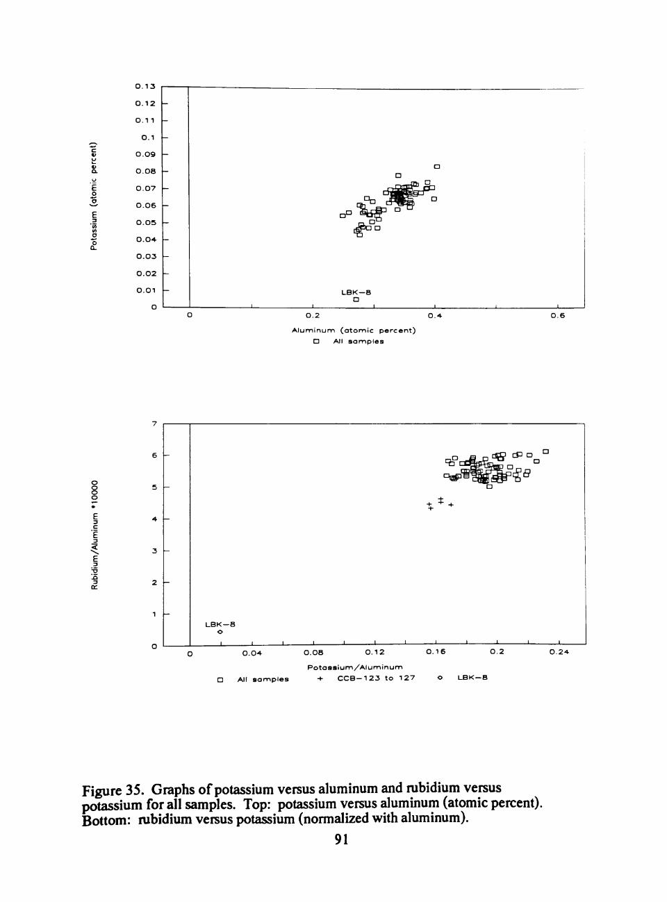
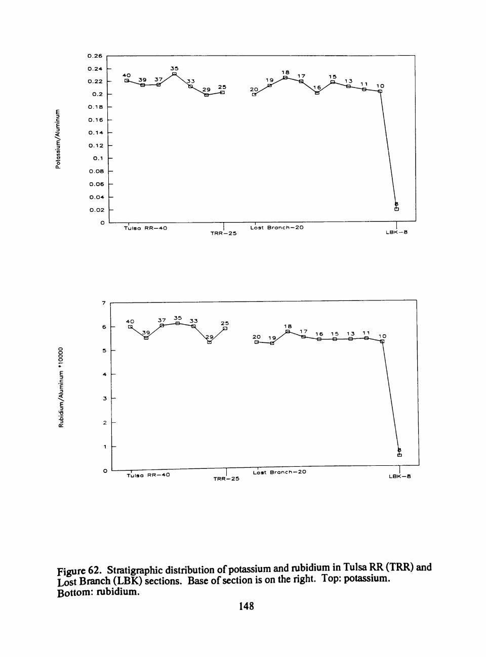
Sodium, potassium, mbidium, iron (total), barium, beryllium, scandium, and
zirconium abundances are exceptionally lower in LBK-8, the Dawson coal, than in the
associated shales. Magnesium, cobalt, and nickel are slightly less in LBK-8. The
concentrations of vanadium, zinc, copper, chromium, strontium, manganese, calcium,
phosphoms, yttrium, and silicon and titanium in the Dawson coal are compzirable to the
associated shales.
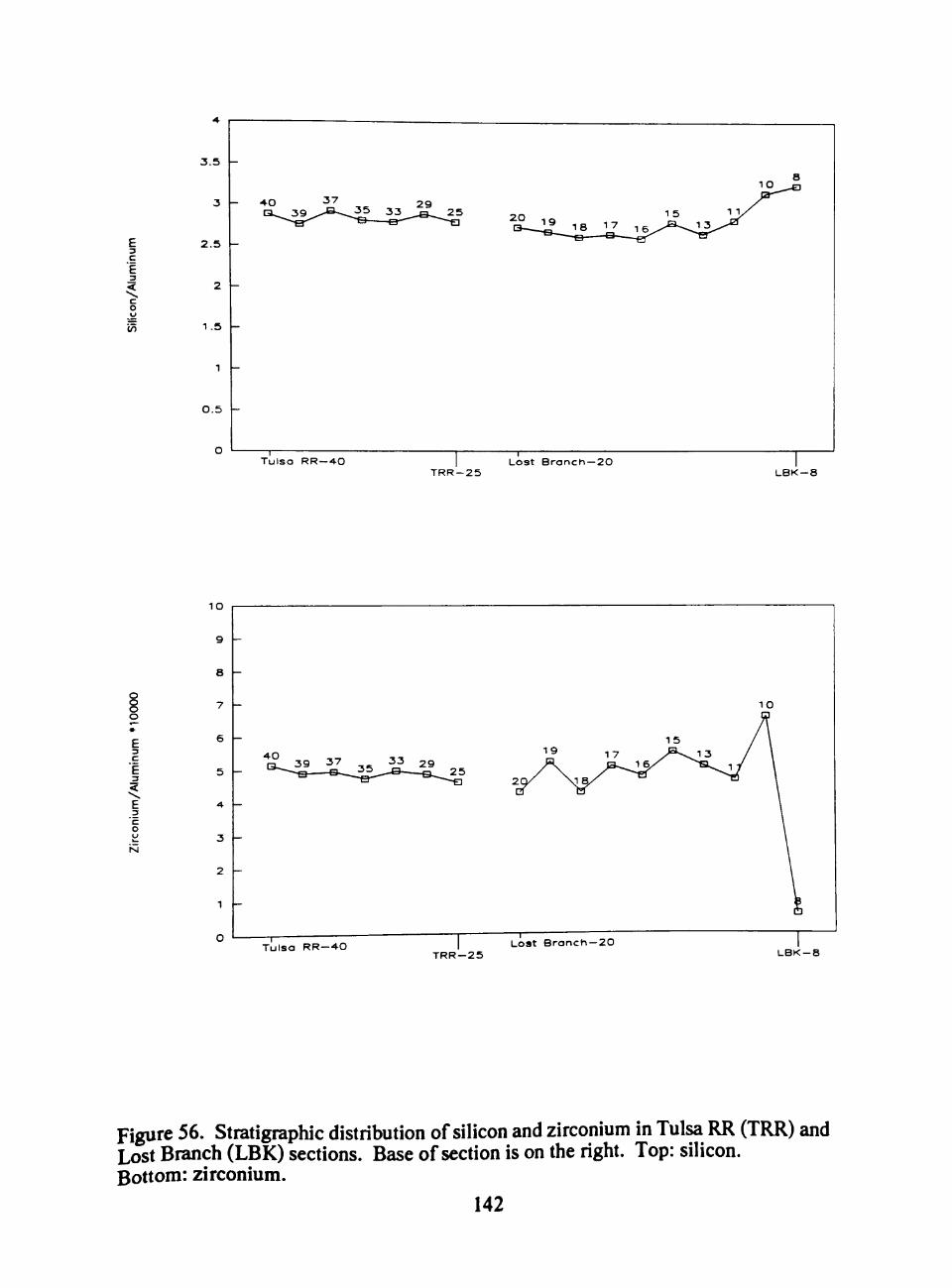
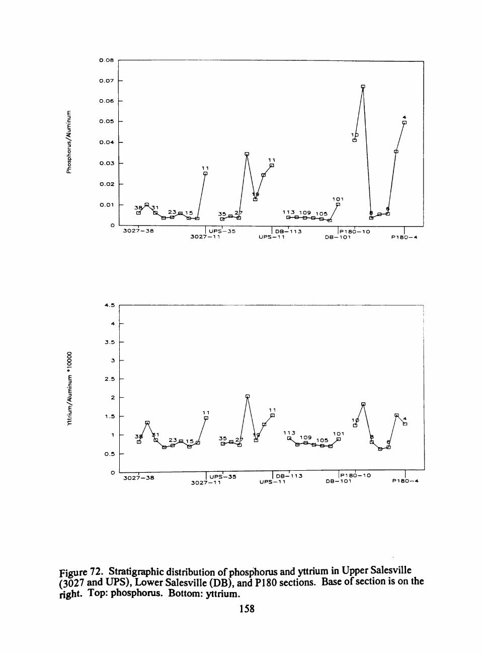
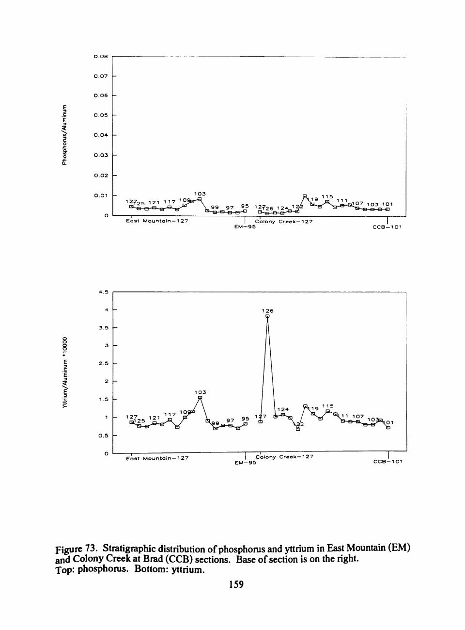
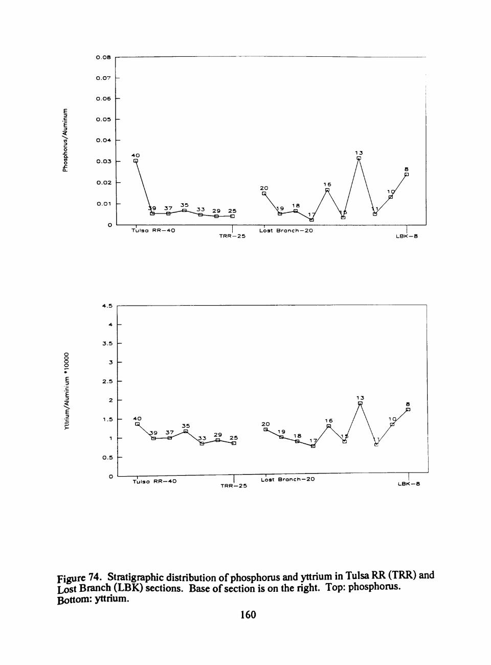
In this section, yttrium and phosphoms show the same distribution pattem with
peaks at LBK-8, 13,16, and 20 that are about 2 or 3 times higher than samples with low
abundances.
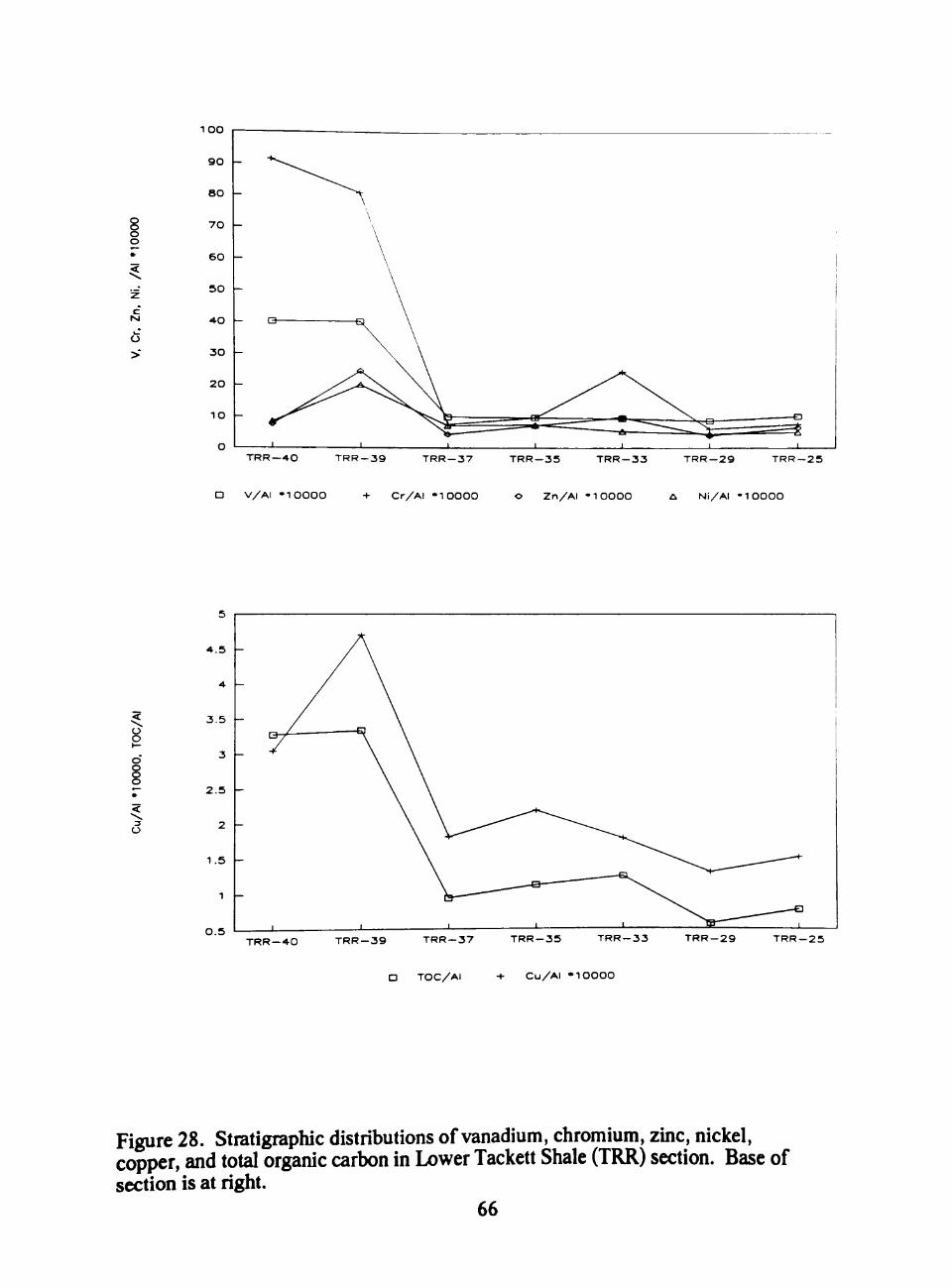
Lower Tackett Section at Tulsa Railroad (TRR)
The TOC varies from 2 to 5 weight percent for the samples TRR-25 to 37. The
basal two samples TRR-25 and 29 contain 2 to 3 weight percent TOC, and TRR-33 to
37 contain about 3.5 to just over 5 weight percent TOC. In contrast, TRR-39 and 40
have TOC values of about 10 weight percent.
Abundances of vanadium and chromium are high only at TRR-39 and 40 (Figure
28). The Ci/Al xlO^ ratio increases eight times from the underiying shale, and the V/Al 53
xlO^ ratio inceases four times. Zinc, copper, nickel, and magnesium show a sharp
increase at TRR-39, but fall to typical levels in TRR-40. Iron (total) and phosphonis are
significantly more abundant only in TRR-40, at the top ofthe black shale. Yttrium
content increases slightly in TRR-40.
Between TRR-29 and TRR-33, both low TOC shales, several elements show
distinct changes in distribution. From TRR-29 to TRR-30, calcium, manganese, and
strontium decrease about 50 percent, but chromium and zinc double in content, and
nickel, copper, and beryllium increase about 10%. Chromium, zinc, and beryllium
decease in TRR-35, but nickel and copper are more abundant.
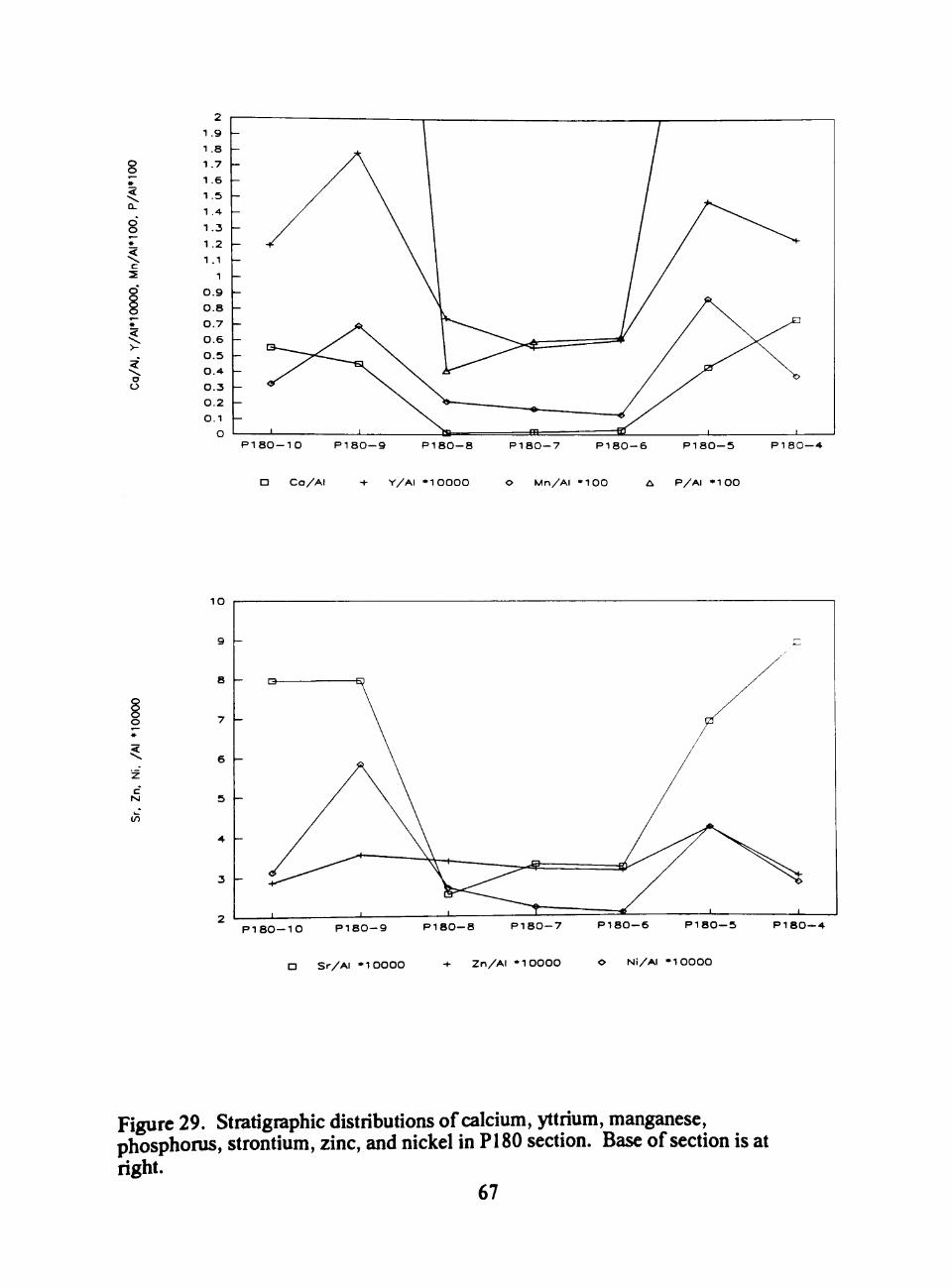
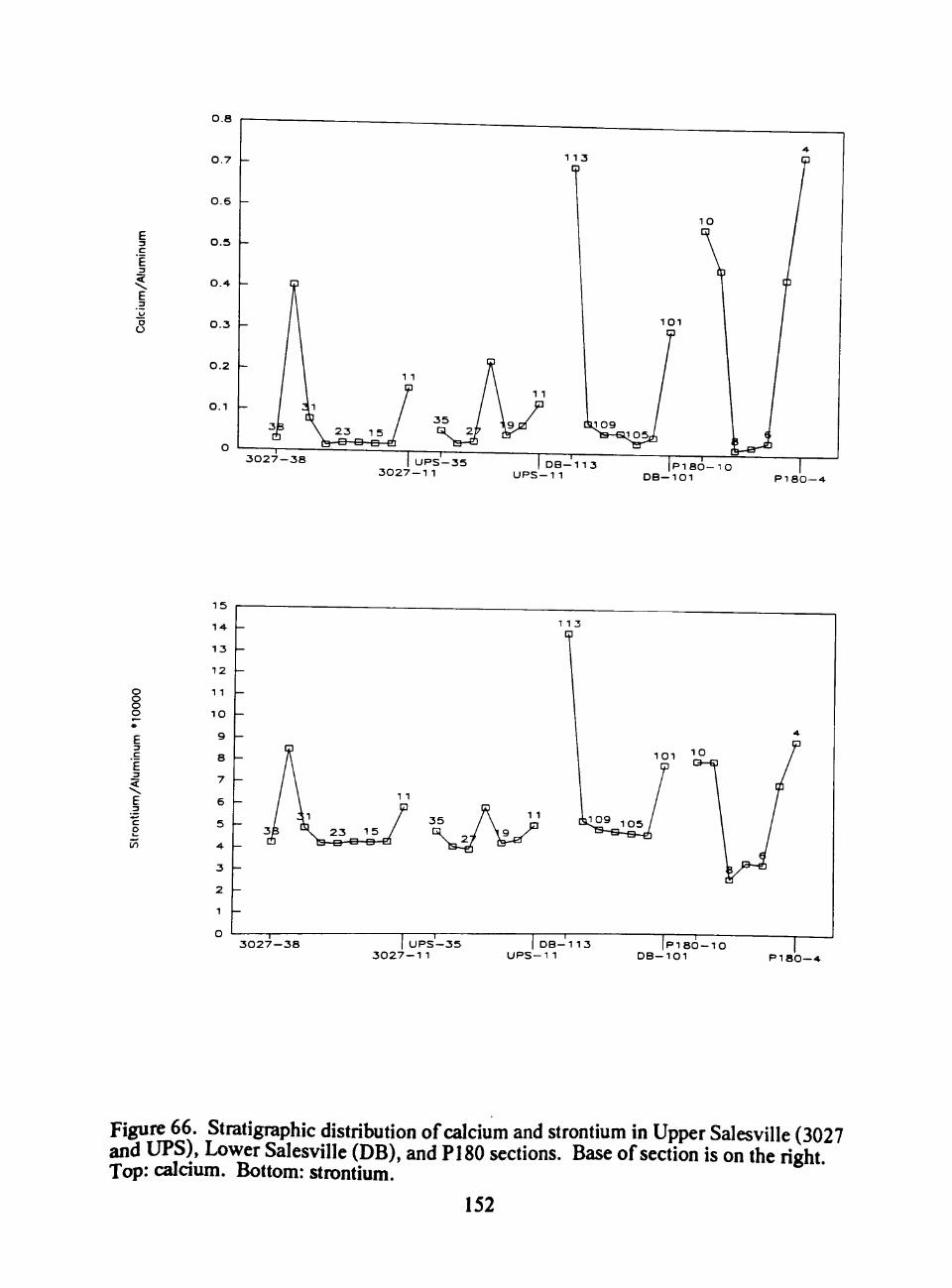
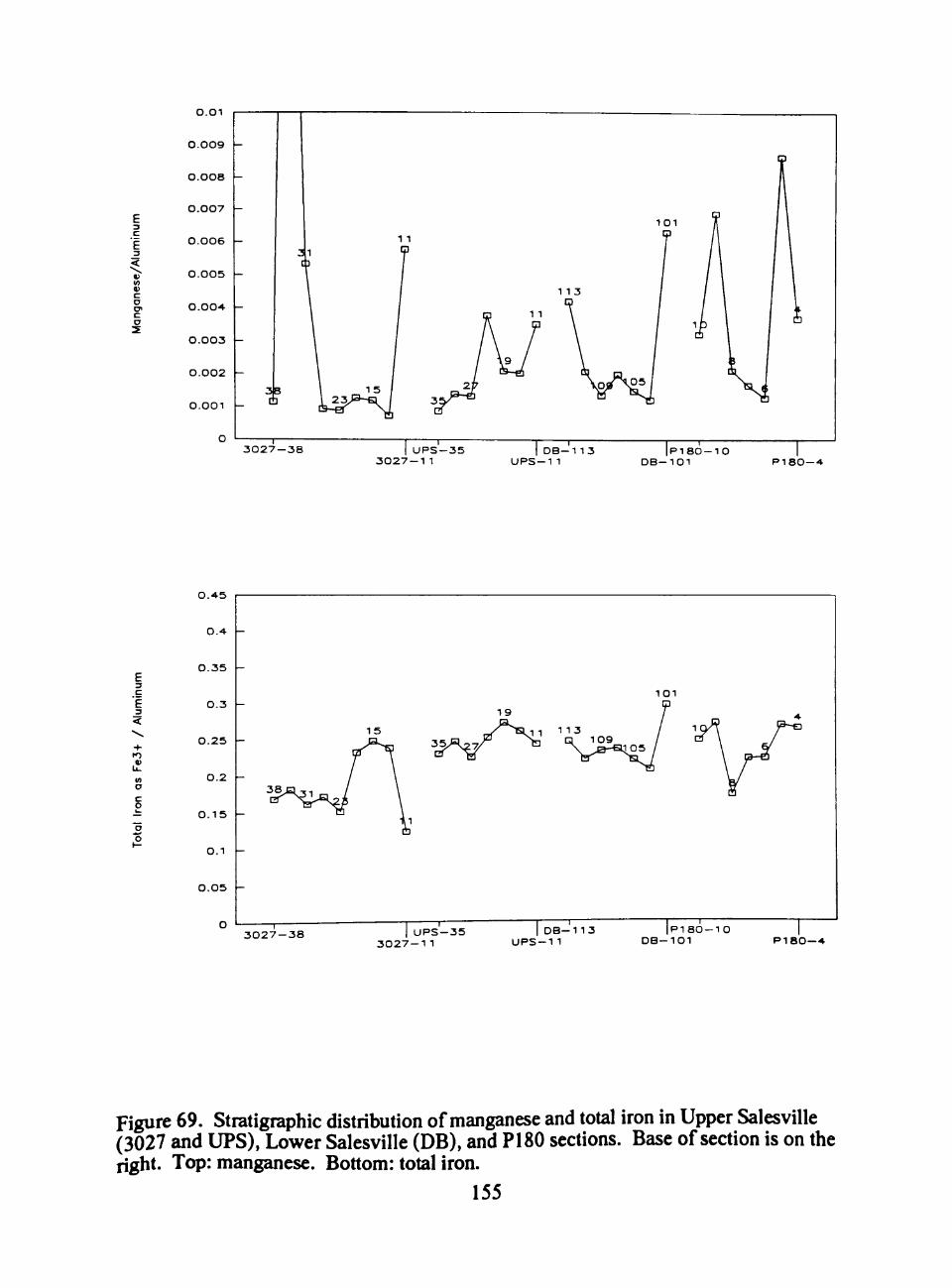
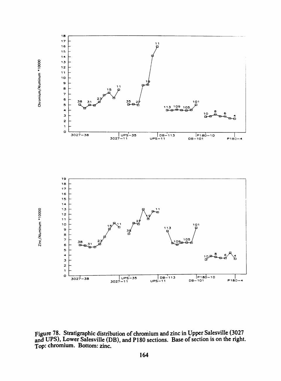
PI80 Section (Permian Bead Mountain Limestone)
The black shale at the base (UNIT 2) and top (UNIT 4) ofthe shale sequence at
PI80 section contains from 1 to 2.5 weight percent TOC, whereas the intervening gray
shale (UNIT 3) contains 1 weight percent or less TOC. Because the weight percent of
aluminum oxide is lower in UNITS 2 and 4, the TOC/Al ratio is two to three times
greater than in UNIT 3. Calcium oxide, probably as calcium carbonate, forms 7 to 11.5
weight percent of samples from UNITS 2 and 4, and less than 0.6 weight percent of
samples in UNIT 3. The Ca/Al ratio in UNITS 2 and 4 is about ten times that in UNIT
3 (Figure 29).
Strontium shows higher abundance in UNITS 2 and 4, the Si/Al xlO^ ratio
increasing about four times that in UNIT 3. Magnesium increases at UNIT 2 only, the
Mg/Al ratio increasing one and a half times. Cobalt, nickel, yttrium, manganese, and
possibly iron (total) and phosphoms, show the same distribution pattem , with high
abundances at P180-5 in UNIT 2 and at P180-9 in UNIT 4. The exception to this
pattem is that iron (total) and phosphoms are not low at PI80-4. Silicon, zirconium,
titanium, sodium, mbidium, and vanadium show higher abundances at PI80-8, 9, and 54
10, with a peak at sample P180-8 just below UNIT 4. Potassium content does not
change throughout the section.
55
c t>
t> o.
o o o
c o
O O
2
1 . 9
1 . 8
1 . 7
1 . 6
1 . 5
1 .••
1 . 3
1 . 2
1 .1
1
0 . 9
0 . 8
0 . 7
0 . 6
0 . 5
O . *
0 . 3
0 . 2
O . I
o
-—
1 1
1 1
1 1
1 1
1 1
1 1
1 1
1 1
~~
D D
i ° D
1 1 1 1 1 1
D
1 1 1 1 1 1
O
a
1 1 1 1 1
D
1 1 1
0 . 2 0.4- 0 . 6 0 . 8 1 1 . 2 1.4.
T i t r a t i o n O r g a n i c C a r b o n ( p e r c e n t )
1 . 6 1 . 8
(per
cent
) C
arbo
n O
rgan
ic
LECO
2 4
2 2
2 0
1 8
1 6
1 4
1 2
1 0
8
6
4
2
0
LBK —1 8 O
LBK — 1 8
L B K - 1 7
a
L B K - 1 5 D
L B K - 1 3 LBK — 1 9 a
L B K - 1 1
n
1 2 1 6 4- 8
T i t r a t i o n O r g a n i c C a r b o n ( p e r c e n t )
a d j u s t e d LBK — 1 8 O o r i g i n o i L B K — 1 8
2 0 2 4
Figure 18. Graphs of LECO total organic carbon versus titration total organic caibon. Top: Samples in which the total oiganic carbon is less than two weight percent. Bottom: Samples in which the total organic carbon is more than two weight percent.
56
L 0) n £ c
0)
2 0 >
(0 c 3
6 -
5 -
4 -
2 -
- 1
-
-
-
-
T\
•
DQDD
luiuiu
nncD D
D DD OD D D D
D D D
1 1 1
LBK-8 D
1 1
0 20
Total Organic Carbon (weight percent)
• All samples
40
Figure 19. Graph of Munsell value number N versus total oiganic carbon (weight percent) for all samples. The lower the Munsell value number N, the darker the sample. The LBK-8 is the coal sample.
57
>
o c M
E M - 1 2 5 E M - 1 2 1 E M - 1 1 7 E M - 1 0 9 E M - 1 0 3
Z n / A l • 1 0 0 0 0 + Cr /A I ' 1 0 0 0 0 O Ni /Al - lOOOO
EM—98 T E M - 9 6 | E M - 9 9 E M - 9 7 EM —95
V / A l ' lOOOO
O .O
O O O O
O O
3
o
E M - 1 2 7 I E M - 1 2 3 I E M - 1 1 9 | E M - 1 1 3 | E M - 1 0 5 | E M - 1 0 1 | E M - 9 8 | E M - 9 6 I E M - 1 2 5 E M - 1 2 1 EM—117 EM—109 E M - 1 0 3 E M - 9 9 E M - 9 7 E M - 9 5
C u / A l "lOOOO Co /A I - lOOOO TOC/Al
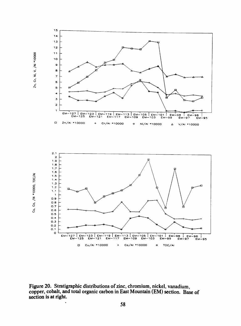
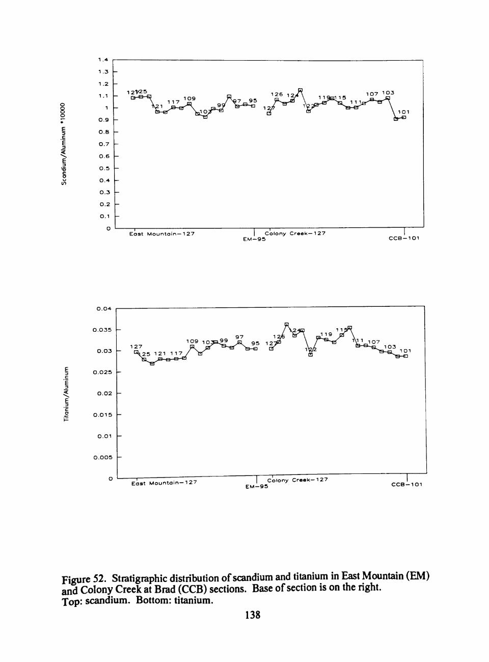
Figure 20. Stratigraphic distributions of zinc, chromium, nickel, vanadium, copper, cobalt, and total organic carbon in East Mountedn (EM) section. Base of section is at right.
58
o
8 o E 3 C
E
c NI
1 5
1 4
1 3
1 2
1 1
1 0
9
8
7
6
5
4-
3
2
1
O
N 3 N 4
N 2 . 5
N 5
EM—127 I E M - 1 2 3 | E M - 1 1 9 | EM—113 | E M - 1 0 5 | E M - 1 0 1 | E M - 9 8 | EM —96 | EM—125 EM—121 EM—117 E M - 1 0 9 E M - 1 0 3 E M - 9 9 E M - 9 7 E M - 9 5
O O O O
E C
•£
u C
Ki
3 0 2 7 - 3 8 | 3 0 2 7 - 3 1 | 3 0 2 7 - 2 3 | 3 0 2 7 - 1 5 | 3 0 2 7 - 1 1 | U P S - 3 1 I U P s ' - 2 3 | U P s ' - l 5 | 3 0 2 7 - 3 5 3 0 2 7 - 2 7 3 0 2 7 - 1 9 3 0 2 7 - 1 3 U P S - 3 5 U P S - 2 7 U P S - 1 9 U P S - 1 1
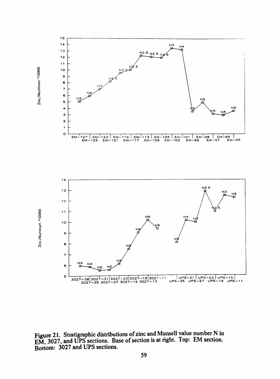
Figure 21. Stratigraphic distributions of zinc and Munsell value number N in EM, 3027, and UPS sections. Base ofsection is at right. Top: EM section. Bottom: 3027 and UPS sections.
59
o o
c
o
8 O •_
>-
o o
D B - 1 1 3 DB—111 D B - 1 0 9 DB—107 DB—105 DB—103 DB—101
• C a / A l •+ Y / A I "lOOOO O Mn/A I " lOO A P/AI • 1 OO
O
<
c
(/)
D B - 1 1 3 D B - 1 1 1 DB—109 OB—107 DB—105 DB—103 D B - 1 0 1
D S r / A I ' lOOOO + 2 n / A I ' lOOOO O Ni /A l • lOOOO
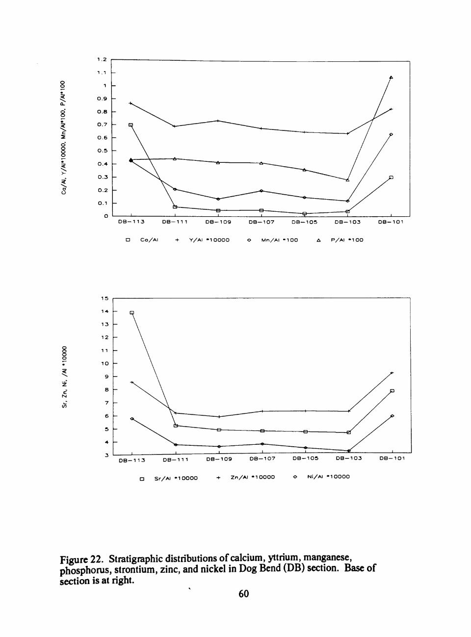
Figure 22. Stratigraphic distributions of calcium, yttrium, manganese, phosphoms, strontium, zinc, and nickel in Dog Bend (DB) section. Base of section is at right.
60
>
c NI
UPS—35 UPS —31 UPS—27 U P S - 2 3 U P S - 1 9 U P S - 1 5 U P S - 1 1
n Z n / A l "lOOOO -t- C r /A I ' lOOOO O N i /A l * 1 0 0 0 0 A V / A l - 1 0 0 0 0
O P
O O O O
O O
3
o
U P S - 3 5 U P S - 3 1 U P S - 2 7 U P S - 2 3 U P S - 1 9 U P S - 1 5 UPS—11
C u / A l ' lOOOO + Co /A I ' 1 0 0 0 0 TOC/Al
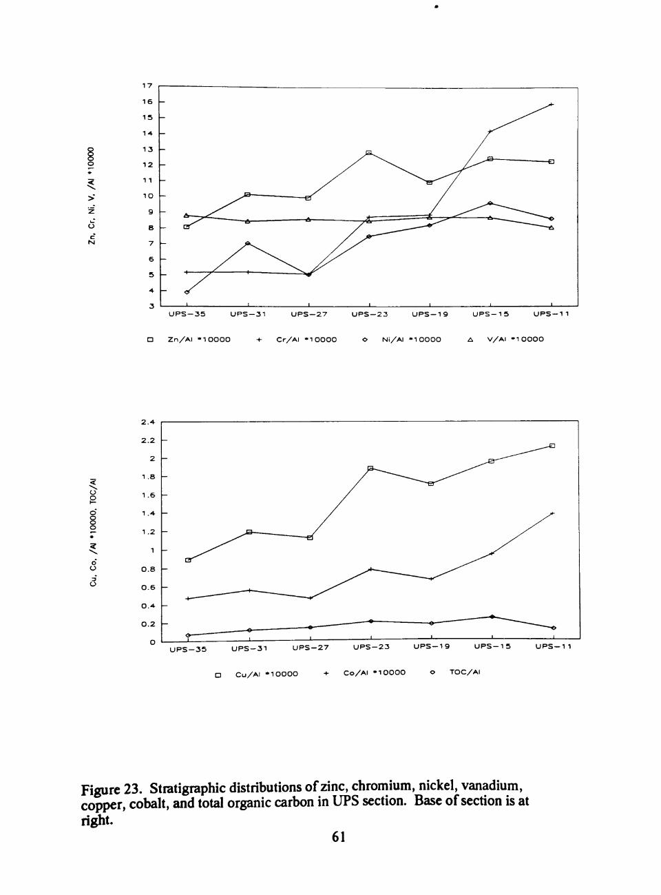
Figure 23. Stratigraphic distributions of zinc, chromium, nickel, vanadium, copper, cobalt, and total organic carbon in UPS section. Base ofsection is at right.
61
o
< 3
o
o c M
1 1
10
9 -
8
7
6
5
4-
3
2
1
O 3027-
• Zn/Al 'lOOOO Cr/AI -lOOOO O Ni/Al -10000
X Cu/Al 'lOOOO
V/Al "lOOOO
1 .1
O O O O
O
1 -
0.9
0.8
0.7
0.6
0.5
0.4
0.3
0.2
0.1
o
Co/AI 'lOOOO TOC/AI
Figure 24. Stratigraphic distributions of zinc, chromium, nickel, vanadium, copper, cobalt, and total organic carbon in 3027 section. Base ofsection is at right.
62
o o
8"
c
>-
o
1 .3
1 .2 -
1 .1
1
0.9
0 . 8
0 .7
0 .6
0 . 5
0.4-
0 .3
0 .2
O.I
O C C B -
C a / A I + Y / A I " lOOOO O M n / A I " l O O P / A I " l O O
1 8
8 o o
c NI
1/1
S r / A I - lOOOO Z n / A l ' 1 0 0 0 0 N i / A l "lOOOO
Figure 25. Stratigraphic distributions of calcium, yttrium, manganese, phosphorus, strontium, zinc, and nickel in Colony Creek (CCB) section. Base ofsection is at right.
63
> c
NJ
P
o o o o
3
o d o o o
n Z n / A l ' lOOOO -t- V / A l ' lOOOO O Cr /A I • 1 0 0 0 0
4 0
3 5 -
3 0 -
2 5 -
2 0 -
15 -
1 0 -
5 -
D N i /A l * 1 0 0 0 0 + C u / A l ' 1 0 0 0 0 O TOC/Al
Figure 27. Stratigraphic distributions of zinc, vanadium, chromium, nickel, copper, and total organic carbon in Type Lost Branch (LBK) section. Base of section is at right.
65
1 0 0 00
00
— « •
^
Ni.
Zn.
Cr.
>
9 0
BO
7 0
6 0
5 0
AO
3 0
2 0
1 0
TRR—40 TRR—39 T R R - 3 7 TRR—35 T R R - 3 3 TRR—29 TRR—25
D V / A l ' lOOOO + Cr /A I » 1 0 0 0 0 O Z n / A l ' lOOOO £i N i /A l - 1 0 0 0 0
P
O O O O
3
o
4 . 5 -
3 . 5
0 . 5
2 . 5 -
1.5 -
TRR—40 T R R - 3 9 T R R - 3 7 T R R - 3 5 T R R - 3 3 T R R - 2 9 T R R - 2 5
D TOC/Al + C u / A l • 1 0 0 0 0
Figure 28. Stratigraphic distributions of vanadium, chromium, zinc, nickel, copper, and total organic carbon in Lower Tackett Shale (TRR) section. Base of section is at right.
66
o o
a.
8 •_
o o
P 1 8 0 — 1 0 P 1 8 0 - 9 P 1 8 0 - 8 P 1 8 0 - 7 P 1 8 0 - 6 P 1 8 0 - 5 P 1 8 0 — 4
• C o / A I Y / A I ' 1 0 0 0 0 Mn /A I ' l O O P/AI ' l O O
1 0
O
<
c NI
m
P I 8 O - 1 0 P 1 8 0 - 9 P 1 8 0 - 8 P 1 8 0 - 7 P 1 8 0 - 6 P 1 8 0 - 5 P 1 8 0 — 4
D S r / A I • 1 0 0 0 0 + Z n / A l - 1 0 0 0 0 O Ni /Al • 1 0 0 0 0
Figure 29. Stratigraphic distributions of calcium, yttrium, manganese, phosphorus, strontium, zinc, and nickel in PI 80 section. Base ofsection is at right.
67
coaly shales of UNIT 6 (CCB-123 to 126), also have higher concentrations of silicon
and zirconium. The upper three samples ofthe Permian shale (P180-8, 9, and 10) have
more silicon and zirconium than the lower four samples. The higher contents of silicon
and zirconium in these samples may be due to the presence of additional detrital quartz
and zircon. Slightly higher amounts of titanium in these samples suggest that titanium-
bearing minerals such as ilmenite and mtile may also be more common.
LBK-8, which is a coal, is strongly depleted in scandium and zirconium relative
to the marine shales of all the sections. When compared to the marine shales of all the
sections, LBK-8 has a typical concentration of titanium and slightly more silicon.
Kaolinite, the predominate clay mineral in coals, has a higher silicon/aluminum ratio
than illite. Terrestrial plants may take up titanium, and coal contains significant titanium,
the titanium being associated with the organic matter (Milnes and Fitzpatrick, 1989).
The low abundance of zirconium may be due to an absence of non-clay detrital particles.
Also, plants do not seem to accumulate zirconium (Milnes and Fitzpatrick, 1989).
Scandium in source rocks is weathered to scandium hydroxide which is more
soluble than aluminum hydroxide (Rankama and Sahama, 1950). Thus, aluminum is
less easily leached than scandium (Curtis, 1972). During weathering, clay minerals are
formed, and aluminum is one ofthe major elements of clays. While aluminum
accumulated as part ofthe clay minerals, the scandium was not deposited in the detrital
sediment in LBK-8. Scandium may correlate with total iron in shales because scandium
hydroxide coprecipitates with ferric hydroxide (Norman and Haskin, 1968), or the
scandium may replace ferrous ion (Curtis, 1972). The data in this sttidy show that
scandium does not correlate with total iron.
Most ofthe samples have Bc/Al xlO^ ratios varying from 0.80 to 0.90 (Figures
57, 58, and 59). The Dawson Coal (LBK-8) contains little beryllium (ratio less than
0.40), and the sample from the overiying shale (LBK-10) has a ratio near 0.70. The 69
marginal marine shale at East Mountain (UNIT 1) has a ratio less than around 0.80, as
does the sample from UNIT 7 (CCB-127) at the top ofthe Colony Creek Shale. In the
black shales at the Tulsa Railroad Cut and the Type Lost Branch slightly higher than
average abundances of beryllium (greater than Bo Al xlO^ ratio of 1.00) are present.
The greatest abundance of beryllium (Be/Al xlO^ ratio =1.25) occurs in one sample of
the carbonaceous shale near the top ofthe Colony Creek Shale (CCB-126 in UNIT 6).
Beryllium typically occurs in detrital clays where it substittites for silicon and
aluminum in clay minerals (Rankama and Sahama, 1950; Vine and Tourtelot, 1970).
The weathering and sedimentary chemistry of beryllium is similar to that of aluminum
(Goldschmidt, 1958; Kretz, 1972).
Degree of Weathering
The source rocks ofthe shale samples in this study were probably subjected to
intense weathering and erosion caused by heavy and frequent rainfall, because
Pennsylvanian North America was at the equator. The high equatorial temperature
facilitated chemical breakdown ofthe source rock minerals. The terrigenous clastic
sediments that travelled along the continental surface via mnoffs and rivers and reached
the marine depositional areas were already highly weathered before deposition. The
weathering index and the chemical index of alteration presented below are ways of
measuring the degree of weathering ofthe source rock minerals into mineral weathering
products before those products setded into the sediment and underwent transfomiation
into shale.
The degree of compositional mamrity ofthe shales in this smdy can be
approximated using a diagram (the weathering index graph) in which the ratio
[(CaO+Na20+K20)/(Al203+CaO+Na20+K20)] is plotted against the ratio
[(Si02+CaO+Na20+K20y(Al203+Si02+CaO+Na20+K20)l (Kronberg and Nesbitt,
70
1981). This index was origmally developed to detennine the degree of weathering of
minerals in soil profiles, but should be applicable to detrital materials in shales derived
from terrestrial weathering.
The y-axis on the weathering index graph (Figure 33) represents the breakdown
of feldspars and the accumulation of clay minerals (measured from 0 to 1). The x-axis
represents the accumulation of Si02 (measured from 0 to 1) or the accumulation of
AI2O3 (measured from 1 to 0) (Kronberg and Nesbitt, 1981). In plotting the
weathering index graph, CaO is not used because, in this sttidy, the amount of CaO in
silicates is not known. Most ofthe calcium in the shales in this sttidy appear to be
associated with carbonates, not silicates.
No significant differences in the weathering index exist among the shales in this
study. Almost all the samples plot around 0.19 on the y-axis and 0.85 on the x-axis
(Figure 33). This plot area is near to the compositions of illite, montmorillonite,
kaolinite, and quartz (Kronberg and Nesbitt, 1981) on the mineral distribution graph,
and is also near to the point on the weathering graph where the weathering is
approaching maximum. The coal (LBK-8) at the Type Lost Branch section, however, is
from a more highly weathered source, and, according to the weathering graph, has more
kaolinite and quartz.
Comparison of aluminum oxides with oxides of calcium, sodium, and potassium
provides a measure of chemical alteration that had occurred to produce the clay minerals
in shales. The chemical index of alteration (CIA) is based on the degree of change from
original feldspar mineral to final product, kaolinite clay (Nesbitt and Young, 1982):
CIA = [ AI2O3/(AI2O3 + CaO + Na20 + K2O ) 1 xlOO.
During chemical weathering, the calcium, sodium, and potassium of feldspars go into
solution while the aluminum and silicon form clays. The greater the degree of chemical
weathering, the less the abundances of calcium, sodium, and potassium, and the higher
71
the CIA value. In the CIA graphs (Figure 34), CaO has been omitted, as explained
above for the weathering index graph.
Although the samples are from different geographical areas and stratigraphic
levels, they have almost the same degree of chemical alteration (Figure 34). There are
slight differences in CIA values among each series of samples, but within each section
there is little change in CIA values. The samples have CIA values ranging from 77
percent to 85 percent, within the illite and montmorillonite range (Nesbitt and Young,
1982). The coal (LBK-8) plots at 97 percent which is significantly above the illite range
and is near to the kaolinite value of 100 percent.
The potassium atomic percent in the samples correlates with the aluminum
atomic percent (Figure 35). The positive correlation of potassium with aluminum may
be due to the possibility that both elements are constituents of illite (Murray, 1954;
Degens et al., 1957; Cubitt, 1979; Dabard and Paris; 1986). The potassium ion is held
tightly in the illite in ancient shales so it is a fixed ion that is not easily exchangeable with
other cations (Cody, 1971); potassium in the samples is therefore assumed to be largely
held in illite.
Rubidium content is rather constant for the samples (Figures 36, 60, 61, and
62). A plot of RVAl xlO^ versus K/Al (Figure 35) suggests that the mbidium is
substituting for potassium in illitic clays in the samples, assuming all the potassium is in
the illite. Rubidium is not found in independent mbidium minerals, but is taken up by
potassium-bearing minerals like illite during weathering. Rubidium easily substimtes
for potassium because the mbidium and the potassium ions have similar ionic radii and
similar ionic potential (Rankama and Sahama, 1950). Rankama and Sahama (1950)
reported a Rb:K ratio of 0.011 for argillaceous sediments. The samples in this smdy
have a Rb:K ratio of about 0.004. The low potassium and mbidium abundances in
LBK-8 coal are probably due to more intense weathering resulting in a higher proportion 72
of kaolinite. The same may be tme ofthe coaly shales of CCB-123 to 126 of UNIT 6
and the daric gray shale CCB-127 of UNIT 7.
Because there is little variation in the potassium content ofthe shales (Figures
36, 60, 61, and 62), the differences in the weathering index and chemical index of
alteration is due primarily to changes in sodium content. Sodium content appears to be
very erratic. Greater differences exist among the sections than among the samples in
each section (Figures 63, 64, and 65). The two sections ofthe Upper Salesville black
shale (3027 and UPS) display strikingly different pattems of sodium content. The
reason for the distribution is not clear. Perhaps the sodium was not retained uniformly
during dewatering ofthe shales.
Elements Associated With Calcium Carbonate
Many cyclothems have a basal transgressive unit that consist of a limestone or a
calcareous sandstone. Near the top ofthe cycles, a regressive shallow-water carbonate
unit may also occur. Calcareous skeletal debris is present in the shales to varying
degrees, commonly adjacent to the carbonate units, and may also be common in shales
that accumulated in shallow-water aerobic envirormients.
Shale samples adjacent to carbonate-rich units have higher concentrations of
calcium due to their greater content of calcium carbonate (Figures 66, 67, and 68). This
occurs in the Dog Bend section adjacent to the trangressive and regressive Hmestones,
above the transgressive limestones at the East Mountain section and the Colony Creeek
section, and above the trangressive calcareous sandstone at the upper Salesville sections
(UPS and 3027). Similariy, the shale adjacent to the carbonates in the Permian section
(PI80) also contains a higher calcium content.
The peak in calcium abundance in UNIT 5 at section CCB, (samples CCB-115
through 121), corresponds to a significantly greater concentration of skeletal debris as 73
determined by wet sieving ofthe shales. Other variations in calcium content in the
shales are not as easily explained. Isolated peaks in the upper Salesville Shale (UPS-23
and 3027-35) and flucttiations of calcium in sections TRR and LBK cannot be readily
attributed to the causes discussed above, but are also believed to be due to variations in
the proportion of calcium carbonate in the samples.
Strontium is a common trace element in carbonate units because it readily
substimtes for calcium in aragonite. In samples in this smdy, strontium abundance
(Figures 66, 67, and 68) is higher in every sample with elevated calcium, suggesting
that the strontium is associated directly with calcium carbonate in these samples. Several
other samples, however, possess a high concentration of strontium and a low
concentration of calcium. Samples from the carbonaceous marginal marine shale at East
Mountain (UNIT 1; EM-95 through 99) and the Colony Creek Shale (UNIT 6; CCB-
123 through 126) tend to have elevated amounts of strontium, especially as compared to
calcium. The shale below the marine black shale, and above the Dawson coal, at the
Type Lost Branch (LBK-10 in UNIT 2) also has high strontium and low calcium
abundances.
Variations in the abundance ofmanganese (Figures 69, 70, and 71) parallel
variations in calcium abundance in a majority of samples, and manganese is thought to
be held largely in carbonates, phosphates, and oxides. However, in the high TOC
samples at the Type Lost Branch (LBK-18, 19 , 20) manganese remains constant,
although calcium sharply decreases.
Magnesium (Figures 63, 64, and 65) does not show a clear correlation with
calcium. Magnesium abundances are probably related to other chemical phases in
addition to calcium carbonate. Little variation in the Mg/Al xlO* ratio occurs in the low
TOC samples, ranging from 0.10 to 0.15. Minor peaks occur in the maximum
transgressive shale at the East Mountain section, the Upper Salesville sections (UPS and 74
3027), and the Colony Creek section. One sample in the Upper Salesville 3027 section
(3027-35) has an unusually high ratio, 0.40. The marginal marine shale at East
Mountain (UNIT 1) and the carbonaceous shale at the top ofthe Colony Creek shale
(UNIT 6 and 7) have lower ratios around 0.05 to 0.07. In the high TOC shales, (LBK
and TRR sections) accumulation of magnesium seems to be to the same degree as in the
low TOC shales.
The abundance of barium (Figures 57, 58, and 59) in the shales is relatively
constant, with most values ofthe Ba/Al xlO^ ratio falling between 7.5 to 8.5. Three
samples in which barium is higher are samples with peaks in calcium abundance (DB-
101 and 113; CCB-119). The other samples with high calcium lack a corresponding
increase in barium. The Dawson coal (LBK-8) has an unusually low barium content.
Inorganic barium occurs in illite, substituting for the potassium (Murray, 1954; Nicholls
and Loring, 1962; Cubitt, 1979), and biogenous barium occurs in carbonates (Goldberg
and Arrhenius, 1958; Chester, 1965).
In samples with low values of TOC, changes in phosphoms abundance (Figures
72, 73, and 74) generally parallel changes in calcium abundance. The similarity of
phosphoms highs and lows with those of calcium suggests that phosphoms may be
connected with calcium due to the presence of apatite [Ca3(P04)2] or a carbonate-
phosphate phase. In the high TOC samples, phosphoms does not correlate with
calcium. Samples of marginal marine shale at East Mountain (EM-95 to 99 in UNIT 1)
and at the Colony Creek section (CCB-123 to 127 in UNITS 6 and 7) contain slightly
more than half the phosphoms found in the samples of marine shale at these sections.
The Y/Al xlO* ratios for most samples range from around 0.7 to 1.0 (Figures
72, 73, and 74). The yttrium highs and lows generally follow those of phosphorus,
suggesting that the yttrium is occurring in the phosphates (Rankama and Sahama,
75
1950). There is no phosphorus peak corresponding to the extremely high yttrium peak
in CCB-126, the carbonaceous marginal marine shale.
Organic Carbon, Sulfur, Iron, and Manganese
Organic Carbon
In sediments with high organic matter content, oxygen is depleted during
decomposition of organic matter producing anaerobic conditions. No oxygen is then
available to oxidize settling organic matter which then accumulates in the sediment.
Essential transition metals (discussed under the subheading "Essential Transition
Metals**), which are transition elements essential for life and are associated with organic
matter, accumulated in proportion to the organic matter. Thus in high TOC shales, the
abundance of essential transition metals tend to correlate with the abundance of TOC.
Also, the low redox potential (low Eh) in the environment of deposition ofthe high
TOC shales was low enough to produce H2S, with resultant formation of pyrite. The
high TOC shales in this sttidy have TOC/Al ratios of above 1.2.
Using a TOC/Al ratio above 1.2 as a criterion for high TOC shales (Figure 50),
the Kansas shales LBK-13, 15, 16, 17, 18, 19, and the Oklahoma shales TRR-39, 40,
are high TOC marine shales. Their essential transition metal contents tend to correlate
with TOC content. The coal LBK-8 is a high TOC shale as its TOC/Al ratio is above
1.2. However, despite its high TOC content, the coal has a low abundance of essential
transition metals. What is applicable to high TOC marine shales, namely high
abundances of essential transition metals are associated with high TOC and vice versa, is
not applicable to high TOC coal.
The envirormient of deposition of sediments with low organic matter content
probably ranged from dysaerobic to near aerobic. The extent of oxidation ofthe organic
matter varied because ofthe flucttiation ofthe redox potential. Thus in low TOC shales 76
the abundances of essential transition metals do not correspond with the increase or
decrease of TOC due to the variability of environmental conditions.
Using TOC/Al ratio below 1.2 as a criterion for low TOC shales (Figures 48 and
49), all the Texas marine samples (EM, CCB, DB, UPS, 3027) are assigned to this
group. The marginal marine carbonaceous shales of Colony Creek at Brad CCB-123 to
127 of UNITS 6 and 7, and the marginal marine shales ofthe Permian PI 80 section
have variable TOC/Al ratios. The Kansas samples LBK-10, 11, 20, and the Oklahoma
samples TRR-25, 29, 33, 35, 37, can be considered low TOC shales, because they have
TOC/Al ratios of below 1.2. LBK-11, with TOC/Al ratio of 1.4, is on the borderline
between high and low TOC shales.
Sulfur
In the low TOC samples, the S/Al values do not correlate with total Fc/Al values
or with TOC/Al values. However, in the high TOC samples (LBK-11, 13,15,17,18,
and 19), the S/Al values correlate well with total Fe/Al values. The slope ofthe graph is
generally parallel to the stoichiometric FeS2 (pyrite) slope (Figure 26). The negative y-
intercept and the positive x-axis intercept indicate that not all the total iron is in the
pyrite. Some iron may be the constituent of organic matter or substituted in clay
minerals, or may be adsorbed onto the organic matter or onto the clay minerals. In high
TOC samples, pyrite was identified in thin sections and by X-ray diffraction.
In the high TOC samples, the S/Al values also correlate well with TOC/Al
values. The regression line for LBK-13, 15, 17, and 19 values (Figure 26) passes
through the x-axis suggesting that pyrite formation depends upon a certain level of TOC
accumulation to cause a favorable low redox condition
The degree of pyritization (DOP) is a way of determining the level of reaction of
unbound reactive iron with hydrogen sulfide (Leventhal and Taylor, 1990). The DOP is 77
the ratio of pyrite iron to total iron, the total iron being the acid-soluble iron plus pyrite
iron (Raiswell and Bemer, 1985; Schultz, 1989). The degree of pyritization is an
indication of oxygenation level at the sediment-water interface. A DOP of 0.45 divides
aerobic and dysaerobic environments, and a DOP of 0.75 divides dysaerobic and
anaerobic conditions (Raiswell et al., 1988; Schultz, 1989). For marine sediments, if
percent pyrite sulfur correlates positively with percent organic carbon and the graph
passes through the origin, then pyrite formation depends on organic carbon
accumulation (Raiswell and Bemer, 1985). If the graph has a positive intercept on the
pyrite sulfur axis, the relation of DOP versus organic carbon could distinguish whether
pyrite formation is limited by organic carbon or by unbound reactive iron (Raiswell and
Bemer, 1985). As acid-soluble iron was not determined in this smdy, the DOP value
could not be obtained.
The pE is the negative logarithm ofthe electron concentration in moles per liter.
The Eh (redox potential) is a measure of a solution's ability to supply electrons for
chemical reaction. Eh and pE are related by the equation Eh = [(2.303 RT)/F] pE
(Kraskopf, 1955, 1967; Brookins, 1988), where R is the gas constant (0.001987
kcal/mole/degree K), T is the absolute temperature, and F is the Faraday constant
(23.06 kcaWolt-gram equivalent). For 25**C, T = 298.15°K, and Eh = 0.059 pE.
The Eh of a solution at non-standard condition is given by the Nemst equation
Eh = E'*+[(2.303 RTy(nF)]log{([Y]y[ZF)/([B]b[D]d)}, where E° is the standard
potential, and n is the number of electrons given by one atom to another (Kraskopf,
1955, 1967; Brookins, 1988). The symbols B and D are the reactants, Y and Z are the
products, in the general chemical equation bB+dD = yY+zZ. The Eh-pH stability field
diagrams of selected metal sulfides are shown in Figures 37, 38, 39,40, 41,42.
78
Iron and Manganese
The stratigraphic distributions of iron (total) and manganese are shown in
Figures 69, 70, and 71. In low TOC shales (East Mountain, Colony Creek, upper and
lower Salesville, and PI80), total iron and ferrous iron abundances pooriy reflect the
redox conditions of marginal and normal marine.depositional environments. The total
iron content is erratic and does not show a relationship with manganese content. The
ferrous iron/total iron ratio does not have any correlation with stratigraphy. The
manganese content of these shales parallels variations in the calcium abundance. The
manganese may be incorporated into the sediment as carbonate, phosphate, or hydrated
oxide. The increase in manganese content with the abundance of skeletal calcium
carbonate in these sections suggests oxidizing conditions. Many ofthe carbonate
skeletal microfossil grains show thin oxide coatings in these shales. Both the
manganese and the skeletal calcium abundances may reflect the dysaerobic-near aerobic
transition zone ofthe depositional environment better than the total iron abundance.
Both iron (total) and manganese contents are slightly lower in the marginal
marine shales than in the normal marine samples of East Mountain and Colony Creek.
Other than that, the iron (total) and manganese contents are variable and erratic. The
ferrous iron/total iron ratios in the marginal East Mountain samples (EM-95 to 99) are
about half that ofthe normal marine East Mountain samples (Appendix B). The Colony
Creek marginal marine carbonaceous shale samples (CCB-123, 125, and 126 in UNIT
6) have about twice the ferrous iron/total iron ratios ofthe normal marine Colony Creek
samples (Appendix B). Marginal marine East Mountain shales have less ferrous iron
than normal marine East Mountain shales because they were deposited under higher
redox conditions. The carbonaceous Colony Creek shales, due to higher TOC content,
were deposited under lower redox conditions than the normal marine Colony Creek
79
shales and the ferrous iron content is correspondingly higher. The normal marine East
Mountain samples show no significant variation in total iron content.
The iron (total) and manganese abundances in the high TOC shales are about the
same level as in the low TOC shales. There is no correlation of iron or manganese with
TOC in the low TOC shales (Figures 43 and 44). For the high TOC shales, total iron
shows correlation with increase of TOC, whereas the manganese shows no association
with TOC (Figures 43 and 44). When the TOC content was high, the redox potential
was low, and iron was probably locked in the sulfide phase as pyrite. Manganese
sulfide is stable within a very narrow range of Eh (redox potential) and pH, whereas
iron sulfide is stable over a greater range (Garrels and Christ, 1965; Brookins, 1988).
Thus in the depositional environment ofthe high TOC shales, the manganese ions had
diffused away leaving behind the iron which was immobilized in the pyrite solid phase.
The manganese in the high TOC and the low TOC shales is probably a
constiment ofthe organic matter. The slightly higher abundance ofmanganese in some
samples ofthe low TOC shales are associated with carbonate, phosphate, or oxide
phases as explained above. In the low TOC shales, the coal LBK-8 and the CCB
carbonaceous samples have a higher, but still narrow range of total iron abundances.
For the low and high TOC shales, perhaps most ofthe iron was associated with organic
matter when they came into the area of deposition. For the high TOC shales, after
deposition in the sediment, the iron switched from association with organic matter to
association with sulfur; thus the iron, organic carbon, and sulfur seem to correlate with
each other.
Essential Transition Metals
Nutrient elements are chemical elements essential for biological systems to carry
out the life processes of maintenance, growth, and reproduction. Shaw (1960) grouped
80
nutrient elements into essential alkali and alkaline earth metals, essential transition
metals, and essential non-metals. Therefore, essential transition metals are transition
metals that are nutrient elements. The essential transition metals discussed here are
vanadium, chromium, cobalt, nickel, copper, and zinc. The essential transition metals
iron and manganese are discussed under the subheading "Organic Carbon, Sulfur, Iron,
and Manganese.**
Essential transition metals are concentrated to levels exceeding oceanic
abundances in the tissues of marine plankton (Manskaya and Drozdova, 1968;
Krauskopf, 1956). Upon the death ofthe organisms, the metals are remmed to the
environment, either in the form of soluble complexes or locked in particulate organic
detritus. Where the TOC of shales is high, the abundances of essential transition metals
are expected to be correspondingly high. In low TOC samples, the content of essential
transition metals will be lower, but other factors may permit enrichment of some of these
metals above anticipated levels. Clay minerals and iron/manganese oxides may
preferentially scavenge these metals from sea water when plankton productivity is high
and rates of sediment deposition and burial are low. Analyses of shales from outer shelf
settings show that low TOC sedunents may be enriched in some metals like zinc and
chromium (Yin et al., 1989).
Vanadium
The vanadium content is very low in low TOC shales (Figures 75 and 76) and
high in all the high TOC shales (Figure 77), except for the Dawson coal (LBK-8). For
TOC/Al ratios of less than 2, the samples show V/Al xlO^ ratios of around 6 to 10. For
TOC/Al ratio of more than 2 in marine shales, there is a linear relationship (Figure 45).
For each 1 unit increase in TOC/Al ratio, the V/Al xlO^ ratio increases by about 25. The
matter contains relatively little vanadium (Manskaya and Drozdova, 1968; Keith and
Degens, 1959). The interpreted low illite content (see position of LBK-8 in Figure 32
top graph and Figure 33) ofthe clay in the coal, would also explain why the coal has
less vanadium than the shales.
82
Essential Transition Metals in Low TOC Shales
The majority of samples in this smdy are low TOC shales, where the quantity of
oiganic matter will have a small effect on the abundances of essential transition metals.
There is no correlation between abundances of essential transition metals and organic
carbon in low TOC shales (Figure 46).
Chromium. Chromium shows relatively little variation in low TOC shales
(Figures 78 and 79), with the Ci/Al xlO^ ratios varying from 4.5 to 6. At most
sections, the chromium is more abundant at the base ofthe dark gray to black shale that
represents the maximum transgressive interval. At the Upper Salesville section UPS,
there is a steep drop ofthe Cr/AI xlO^ ratio from 15 to 5 higher in the section. At the
Upper Salesville section 3027 and East Mountain secion, the Cr/AI xlO^ ratio drops
from around 6 to 7 in the maximum transgressive shale to 4 higher in the section. At the
Dog Bend and the Colony Creek sections, chromium abundance drops only slightly.
The marginal marine shale at PI 80 shows the lowest ratio of between 2.5 to 3.
Zinc. In general, the marine shales have Zn/Al xlO^ ratios varying widely from
5 to 13 (Figures 78 and 79). The abundance of zinc varies in a manner similar to that of
chromium, but shows a greater range of values. The Zn/Al xlO* ratio decreases from a
maximum value in the maximum transgressive shale interval to lower values higher in
the section. In the Upper Salesville at UPS and 3027 and the East Mountain sections,
zinc content drops sharply. In the Colony Creek at Brad and the Dog Bend sections,
zinc shows a slight decrease. There is more zinc in the upper part ofthe Colony Creek
shale section at Brad and the top sample ofthe shale at the Dog Bend section. These are
the samples that contain higher abundances of elements (calcium and strontium)
associated with carbonates. Two samples with unusually high concentrations of zinc
occur associated with the carbonaceous shale at section CCB (samples 122 and 126).
83
The marginal marine shale at section P180 has low Zn/Al xlO^ ratios of about 3
to 4, comparable to those ofthe marginal marine shale at East Mountain (EM-95 to 99),
which has values of about 3 to 5.
Nickel. Nickel has a somewhat mixed distribution in the low TOC shale
samples, with most values ofthe Ni/Al xlO^ ratio falling between 2 and 4 (Figures 75
and 76). Peaks of nickel occur stratigraphically just above the peaks of chromium and
zinc in the maximum transgressive shale in some sections (Upper Salesville shale at
UPS and 3027, and at East Mountain). In the Colony Creek section at Brad, the
abundance of nickel is only slightly greater in the maximum transgressive shale. Other
significant peaks in nickel distribution occur in samples bearing high calcium, strontium,
and manganese in the Dog Bend section and PI80 section. In the carbonaceous shales
near the top ofthe Colony Creek at Brad (UNIT 6), nickel is also high in some samples,
but near average in others.
In the shale at the top ofthe Colony Creek at Brad (UNIT 7) and the marginal
marine shale in the lower part ofthe East Mountain section (UNIT 1) nickel abundance
falls to its lowest values, Ni/Al xlO^ ratios of less than 1.5, compared to typical values
greater than 2.
Cobalt Most values ofthe Co/AI xlO^ ratio range between 0.4 and 0.8 (Figures
81 and 82). A minor peak occurs in the maximum transgressive shale at the Upper
Salesville sections 3027 and UPS and at East Mountain section. Little regular
stratigraphic variation exists higher in these sections or in the marine shales in Colony
Creek section or the Dog Bend section. Greater abundances of cobalt occur at the top of
UNIT 6 in the carbonaceous shale in the Colony Creek section, and in two samples at
PI 80 (PI 80-5 and 9). The marginal marine shales at the base ofthe East Mountain
section (UNIT 1) have slightly lower Cc/Al xlO^ ratios, less than 0.4.
84
Copper. The Cu//Al xlO^ ratios range between 0.5 to 1.5 for most marine shale
samples (Figures 81 and 82). Minor peaks occur in the maximum transgressive shale at
the East Mountain, UPS, 3027, and perfiaps the Colony Creek sections. Unusually
high values occur in two samples at the 3027 section, where the Cu/Al xlO^ ratio rises
to above 5.5 and 14 at samples 3027-23 and 38, respectively.
Essential Transition Metals in High TOC Shales
There is correlation between the abundances of essential transition metals and
organic carbon in high TOC shales (Figure 47). In the high TOC shales, (LBK and
TRR sections) accumulation of cobalt (Figure 83) seems to be ofthe same degree as in
the low TOC shales (Figures 81 and 82). Nickel and copper abundances (Figures 77
and 83) in the high TOC shales are two to four times larger than in low TOC shales
(Figures 75, 76, 81, and 82). Vanadium, zinc, and chromium (Figures 77 and 80) in
the high TOC shales show abundances that are five to nine times higher than in the low
TOC shales (Figures 75, 76, 78, and 79). Above a certain threshold of TOC/Al ratio
(between 1 and 2), nickel and copper correlate weakly with the TOC , and vanadium,
zinc, and chromium correlate strongly with the TOC (Figure 47).
Although the organic carbon content ofthe shale (TRR-40) at the top of TRR
section shows no change compared to the lower adjacent shale layer, the abundances of
copper, zinc, and nickel decrease, vanadium remains the same, and chromium increases
(Figure 28). From the base to the middle of LBK section, organic carbon and essential
transition metals generally increase, and from the middle to the top ofthe section, they
decrease (Figure 27). At LBK-16, organic carbon, copper, and nickel abundances
hardly change compared to the adjacent layers above (LBK-17) and below (LBK-15)
but zinc, vanadium, and chromium increase.
85
c V 3 CT V
32
30
28
26
24
22
20
18
16
14-
12
10
8
6
4
2
O —r-o I I I I r
0.5 I 1 I 1.5 I 2 I 2.5 0.25 0.75 1.25 1.75 2.25 2.75
Si l icon/Aluminium 3.75
I -^.5 I 4.25 4.75
c V 3 cr V
40
35 -
30
25 -
20 -
15
10 -
5 -
'o I O d04 I 0.d08 I 0.612 I 0.016 I 0.02 I 0.024 I 0.028 | 0.032 | 0.036 | 0.04-0.002 0.006 0.01 0.014 0.018 0.022 0.026 0.03 0.034- 0.038
Ti ton ium/Alu min ium
Figure 30. Frequency histograms of silicon and titanium abundances for all samples. Top: silicon. Bottom: titanium.
86
c v 3 O" V
5 0
4 5
4-0
3 5
3 0
2 5
2 0
15 I -
10
b&A&i
O.I 0 . 2 0 .3 0 . 4 0 .5 0 . 6 0 .7 0 .8 0 .9
S c a n d i u m / A l u m i n i u m * 1 0 0 0 0
1.1 1 .2 1 .3
4 0
3 5 -
3
3 0
2 5 -
2 0 -
15 -
10 -
5 -
2 3 4 5 6 7
Z i r c o n i u m / A l u m i n i u m "lO.OOO
1 0
Figure 31. Frequency histograms of scandium and zirconium abundances for all samples. Top: scandium. Bottom: zirconium.
87
E 3 C
'E _3
E 3
o c
11
1 0
9
8
7
6
5
4-
3
2
1
O
LBK—8
1 i
a^i
<^^
o^o
a
0 . 0 4
a All lov
0 . 0 8 O.I 2
P o t a s s i u m / A l u m i n u m
0 . 1 6 0 . 2 0 . 2 4
TOC s a m p l e s + C C B - 1 2 2 t o 1 2 7 o P 1 8 0 - 4 t o 1 0
X T R R - 2 5 to 3 5 V L B K - 8 . 10 , a n d 2 0 EM—95 to 9 9
8 o o
E 3 C
E _3 < E 3
'c O
• All samples
S i l i c o n / A l u m i n u m
C C B - 1 2 3 t o 1 2 6 O EM —101
V 3 0 2 7 - 1 1 A L B K - 8 X C C B - 1 1 3
Figure 32. Graphs of vanadium versus potassium and zirconium versus silicon. Top: Graph of vanadium versus potassium for all low TOC samples. The LBK-8 is the coal sample. Bottom: Graph of zirconium versus silicon for all samples.
88
0 CM
+ 0 CM D z + 0 CM
<
\
0 CM
+ 0 CM D
z
1
0.9
0.8
0.7
0.6
0.5
0.4
0.3
0.2
0.1
Gibtsite
-e-0 0.2 0.4
Na & K-Felcispars Ca-Felcispars • •
llite D
All Samples
Montmorillonite •
Kaolinite LBK-8
D
0.6 0.8
(Si02+Na20+K20)/(AI203+Si02+Na20+K20)
Quartz
1
Figure 33. Graph of weathering index for all samples. The LBK-8 is the coal sample.
y-axis = [(CaO+Na20+K20y(Al203+CaO+Na20+K20)] X-axis = [(Si02+CaO+Na20+K20y(Al203+Si02+CaO+Na20+K20)l (Kronberg and Nesbitt, 1981).
Note that CaO values are not used in the calculations of weathering index for the shale samples (see text).
89
c «> 3
«>
3 4
3 2 -
3 0 -
2 8 -
2 6
2 4
2 2
2 0
1 8
1 6
1 4
1 2
1 0
8
6
4
2
O o T 1^ T -r 8 I 16 1 2 4 I 3 2 I 4 0 | 48 | 56 | 64 | 72 | 80 | 88 | 96
1 2 2 0 2 8 3 6 4 4 5 2 6 0 6 8 7 6 8 4 9 2 TOO C h e m i c a l I n d e x o f A l t e r a t i o n ( C I A )
< •
o_ c o \^ o
1 — V 5
o X V -o c
"5 u 'E t> .c o
1 0 0
9 8
9 6
9 4
9 2
9 0
8 8
8 6
8 4
8 2
8 0
7 8
7 6
74^
7 2
7 0
—
- " ^ ^ ^ ^ ^ ^
1 , , E M
t S ? r ^ K C S L E , i ^ ^ P t ^ ^
c * L r M ^ ^ • ^ D
P
1 CCB 1 3027 E M C C B
^ n \? ^ M C^Sn D ^ ^
rf!^^ 1
1 DB 1 UPS 3 0 2 7 D B
r ^ C l l ^ ^ I3aJ7«=3XJ
,£1 o p^
C ^ 9 V •
1 P180 1 TRR U P S P 1 8 0
r i ^ oR5^J^ L ^ r r M P
•
1 LBK T R R
D
I LBK
Figure 34. Graphs of chemical mdex of alteration (CL\) for all samples. Top: frequency histogram. Bottom: distribution by sample and section; base ofsection is at right.
CIA = [Al2Oy(Al2O3+CaO+Na2O+K2O)lxl00 (Nesbitt and Young, 1982).
Note that CaO values are not used in the calculations of CL\ for the shale samples (see text).
90
c V 0) a.
E o
E 3
O
0 . 1 3
0 . 1 2 -
O. I 1
O.I I -
0 . 0 9
0 . 0 8
0 . 0 7
0 . 0 6
0 . 0 5
0.04-
0 . 0 3
0 . 0 2
0 . 0 1
O _
LBK—8 D
0 .2
Aluminum (a tomic percent )
• All samples
0 . 4 0 . 6
O
8 o E 3 C '£ _3
E 3
'•U
'.O 3
6 -
5 -
4 -
2 -
^SQ CP D
LBK—8 O
_ L JL.
0 . 0 4
All somples
0 . 0 8 O.I 2 0 . 1 6 0 . 2
P o t a s s i u m / A l u m i n u m
+ C C B - 1 2 3 to 1 2 7 LBK —8
0 . 2 4
Figure 35. Graphs of potassium versus aluminum and mbidium versus potassium for all samples. Top: potassium versus aluminum (atomic percent). Bottom: mbidium versus potassium (normzdized with aluminum).
Figure 36. Frequency histograms of potassium and mbidium abundances for all samples. Top: potassium. Bottom: mbidium.
92
1 1 1
SYSTEM C o - S - C - 0 - H
25*»C. 1 bar
10 12 14
Figure 37. Eh-pH diagram showing stability field of cobalt sulfide (Brookins 1988). The solubility product of cobalt sulfide is (Dean, 1985; Krauskopf, 1967): Mineral Fonnula Solubilitv Pmdnrt jaipurite alpha-CoS 10-20.4 jaipurite beta-CoS 10-24.7
93
SYSTEM C u - C - S - 0 - H 25°C, 1 bar
12 14
Figure 38. Eh-pH diagram showing stability field of copper sulfide (Brookins, 1988). The solubility product of copper sulfide is (Dean, 1985; Krauskopf, 1967): Mineral Formula Solubilitv Product chalcocite Cu2S 10-47.6 covellite CuS 10-35.2
94
UJ
-0.2 —
-0.4 —
-o.e
-0.8 I
Figure 39. Eh-pH diagram showing stability field of iron sulfide (Brookins, 1988). The solubility product of troilite (FeS) is 10-17.2 ny^^ 1985. Krauskopf, 1967). ' '
95
SYSTEM Mn-C-S-O-H 25°C, 1 bar
12 14
Figure 40. Eh-pH diagram showing stability field ofmanganese sulfide
ThcTsolubility product ofmanganese sulfide is (Dean, 1985; Krauskopf, 1967): Mineral Fonnula Solubility Product
Figure 41. Eh-pH diagram showing stability field of nickel sulfide (Brookins. 1988). The solubility product of nickel sulfide is (Dean, 1985; Krauskopf, 1967): Mineral Fonnula Solubilitv Produrt millerite alpha-NiS 10-18-5 millerite beta-NiS 10-24.0 millerite gamma-NiS 10-25.7
97
SYSTEM Z n - 0 - H - S - C 25°C, 1 bar _
Figure 42. Eh-pH diagram showing stability field of zinc sulfide (Brookins. 1988). The solubility product ofzinc sulfide is (Dean, 1985; Krauskopf, 1967): Mineral Formula Solubilitv Produrt sphalerite alpha-ZnS 10-23.8 wurtzite beta-ZnS 10-21.6
98
E 3 C
'E _3 <
M O
C O
2 "5
0 . 3 2
0 . 3
0 . 2 8
0 . 2 6
0 . 2 4
0 . 2 2
0 . 2
0 . 1 8
0 . 1 6
0 . 1 4
0 . 1 2
O.I
0 . 0 8
0 . 0 6
0 . 0 4
0 . 0 2
O
-
:
1 1
1 1 1
1
-
-
-
o
O
D
n
1 1
D °
1 1 1
D
in
1
•
O
]
a
1 1
D
1 1
0 . 2 0 . 4 0 .6 0 .8
Total Organic Carbon / Aluminum
1 .2
E 3 C
'E
<
in
c o
o o
0 . 4
0 . 3 5
0 . 3
0 . 2 5
0 . 2
0 . 1 5
O . I
0 . 0 5
D
D
n
^^
1 i
a
a
1 1
a
•
1
D
•
1 1 1 1 i
L B K - 8 D
1 1 1 1 1 1
4 6 8 1 0
Total Organic Carbon / Aluminum
1 2 1 6
Figure 43. Graphs oftotal iron versus total organic carbon. Top: low TOC shales. Bottom: high TOC shales.
99
F
Alu
min
ui
V M t>
o c (7 IS
0 . 0 1
0 . 0 0 9
0 . 0 0 8
0 . 0 0 7
0 . 0 0 6
0 . 0 0 5
0 . 0 0 4
0 . 0 0 3
0 . 0 0 2 -
0 . 0 0 1 -
-
-
-
D
O
D
a
•
1 1 1 1 1
D
n
a
1
a 1
D
1 1 D 1 1
0 . 2 0 . 4 0 .6 0 . 8
Total Organic Carbon / Aluminum
1 .2
E 3 C
'E 3
V V) V c o o> c o
2
0 . 0 0 3 2
0 . 0 0 3
0 . 0 0 2 8
0 . 0 0 2 6
0 . 0 0 2 4
0 . 0 0 2 2
0 . 0 0 2
0 . 0 0 1 8
0 . 0 0 1 6
0 . 0 0 1 4
0 . 0 0 1 2
0 . 0 0 1
0 . 0 0 0 8
0 . 0 0 0 6
0 . 0 0 0 4
0 . 0 0 0 2
O
-
—
-
-
-
_
1 1
1
1
• a
• D
a
D
a D
1 1
a
D D
D
1 1
n
•
1
D
D
1 1 1 1 1
L B K - 8 O
I J 1 1 1 1
4 6 8 1 0
Total Organic Carbon / Aluminum
1 2 1 6
Figure 44. Graphs ofmanganese versus total organic carbon. Top: low TOC shales. Bottom: high TOC shales.
100
0 o 0 o
E 3 C
I < \ E 3 '•D
D C D >
130
120
110
100
90
80
70
60
50
40
30
20
10
0
LBK-17 +
LBK-15 +
LBK-16 +
LBK-13 +
TRR-39 & 40 LBK-18 + +
LBK-19 +
LBK-8 . + .
0 8 10 12 14 16
Total Organic Carbon / Aluminum
D Low TOC samples + High TOC samples
Figure 45. Graph of vanadium versus total organic carbon for Lower Tackett (TRR) and Type Lost Branch (LBK) shales. The low TOC samples include those of EM, CCB, 3027, UPS, DB, and P180 sections. The LBK.8 is the coal sample.
101
o
O
8 o
o o 3
o
18
1 7
16
15
1 4
1 3
12
1 1
1 0
9
8
7
6
5
4
3
2
1 —
O
16
15
14
13
12 -
1 1
10
9
8
7
6
5
4
3
2 -
a <J> ^
•
0 . 2 0 . 4 0 . 6 0 . 8 1 .2
Total Organic Carbon / Aluminum
V / A l ' lOOOO + Z n / A l - lOOOO O Cr /A I - lOOOO
D
a D
Pa ^ +Jr^»r ° tSb
t o <? o o o -I 1 I
0 . 2 0 . 4 0 . 6 0 . 8 1 .2
Total Organic Carbon / A luminum
D N i /A l "lOOOO -t- C u / A l " 1 0 0 0 0 O Co /A I "lOOOO
Figure 46. Graphs of vanadium, zinc, chromium, nickel, copper, and cobalt versus total organic carbon for low TOC shales. The low TOC shale samples are from EM, CCB, 3027, UPS, DB, and P180 sections.
102
o c M
1 30
120
1 10
100
90
80
70
60
50
40
30
20
10
0
-
-
-
-
-
-
"~
§ 8 1
• -•-0
1
0
D
-t-
1
D
+
0
1
CO
8 1 0
L B K - 8 ' S L.
1 2 1 4 1 6
V / A l Total Organic Carbon / Aluminum
• 1 0 0 0 0 + Z n / A l - 1 0 0 0 0 O Cr /A I " 1 0 0 0 0
O O
O
3 o
4 0
3 5 -
3 0 -
2 5 -
2 0 -
15 -
10 -
5 -
4 6 8 1 0
Total Organic Carbon / A luminum
1 2 1 4 1 6
Ni /A l "lOOOO C u / A l • 1 0 0 0 0 C o / A I • 1 0 0 0 0
Figure 47. Graphs of vanadium, zinc, chromium, nickel, copper, and cobalt versus total organic carbon for high TOC shales. The high TOC shale samples are from LBK section.
103
CHAPTER V
DISCUSSION
The abundances of vanadium, zinc, and chromium have been used to infer the
level of redox potential (Eh) in depositional environments because these elements
accumulate in low redox environments characterized by accumulation of oiganic matter.
Therefore a strong correlation of vanadium, zinc, and chromium abundances with TOC
abundance suggests that the original sediment was deposited in a low redox environment
that allowed preservation of organic matter. Offshore deep-water shales (core shales of
cyclothems) were formed from sediments deposited during maximum transgression.
Organic matter accumulation and preservation during maximum transgression may have
been enhanced by lower redox potential and/or by higher rates of organic sedimentation.
The presence of a thermocline would lower oxygen concentration at the bottom ofthe
water column and enhance development of a lower redox potential. The relative rate of
sedimentation of organic material would also be greater due to lower rate of terrestrial
clastic influx. The accumulated organic carbon may lower the redox potential to a level
favorable for the formation of hydrogen sulfide. Then, iron can be locked in pyrite but
not manganese. The strong association between iron and sulfur is because ofthe
presence of pyrite. Data for the marine shales in this study show that beyond a
threshold concentration of TOC (TOC/Al ratio > 2), vanadium, zinc, and chromium
correlate strongly with TOC. Nickel and copper also correlate with the TOC although
their increase is not as pronounced as that of vanadium, zinc, and chromium. Iron
abundance is high, and correlates with TOC and with sulfur, whereas manganese is low
and does not correlate with TOC. The inference is that these high TOC shales were
deposited in an original sedimentary condition that was anaerobic.
104
For the high organic carbon shales, a slight change in sedimentary redox
condition might affect the content of essential transition metals without affecting the
organic carbon content. The abundances of essential transition metals might decrease or
remain the same compared to the adjacent shale layeis.
Some core shales are low in TOC; their essential transition metals may increase
at maximum transgression even though the organic caibon content shows no
corresponding increase in the same stratum. The essential transition metals decrease as
regression proceeds. The decrease does not correspond with oiganic carbon content.
The relatively small amount of organic matter preserved in these core shales may be due
to loss of organic matter where the redox potential is high enough for more extensive
oxidation ofthe organic matter. The higher redox potential could be due to the absence
of a thermocline. Following rapid transgression, abundances of essential transition
metals in low TOC core shales increase due to longer settling time allowing settling clay
and oiganic particles to scavenge the essential transition metals with greater efficiency.
As deltas prograde, clastic influx dilutes the sediment causing a relative decrease in the
essential transition metals. In low TOC core shales (TOOAl ratio < 1.2) of EM, 3027,
and UPS sections, abundances of essential transition metals zinc, nickel, and chromium
increase steeply from base then decrease gradually. The essential transition metals do
not correlate with the TOC because of unequal accumulation or loss ofthe essential
transition metals and the organic matter during deposition. Although the underlying
sediment may be anaerobic, some oiganic matter may have been oxidized at a dysaerobic
sediment surface layer and so the organic carbon and the essential transition metals do
not accumulate to any great extent. Core shales with sudden increase from base and
gradual decrease towards upper outside shales of some essential transition metals are
from deep water with dysaerobic sediments.
105
Transgressive and regressive limestone beds are normal feamres of many
cyclothems. Although one or both ofthe transgressive and regressive carbonate strata
may be visibly absent in some cyclothems, higher concentrations of caibonate-related
elements may mark the positions in the cyclothems where limestone beds would be
expected. The Dog Bend section, with transgressive and regressive limestone beds,
shows the expected higher concentrations of caibonate-related elements calcium,
strontium, zinc, manganese, phosphorus, yttrium, and nickel in the upper and lower
part ofthe section. The Colony Creek section, with transgressive limestone but no
regressive limestone, shows higher abundances of caibonate-related elements calcium,
strontium, manganese, and zinc in the upper outside shales compared to its core shales.
The upper outside shales contain marine calcareous fossils. In low TOC regressive
shales, the strong association of calcium, strontium, manganese, nickel, phosphoms,
and yttrium suggests that the environment of deposition was near aerobic and was
conducive to the formation of carbonates, phosphates, and hydrated oxides.
Iron and manganese abundances are expected to be high in aerobic sediments (as
insoluble oxides) and low in anaerobic sediments. Iron and manganese are essential
transition metals and their contents would be affected by organic carbon content. In the
low TOC marine shales in this study, the iron and manganese abundances are erratic,
vary widely, and do not correlate with TOC.
Marginal marine shales are from depositional environments that receive marine
oiganic particles from overlying waters, and terrestrial organic and clastic particles from
land. As the marginal marine sediment is open to influence from sea and land, there
may be no distribution pattem of organic carbon and essential transition metals. The
redox condition in the sediment may vary as the oxygen level in the overlying water
varies. The marginal marine shales of CCB have about 2 percent more organic carbon
than the normal marine shales in the same section. The marginal marine shales of EM 106
have similar levels of organic caibon content as the nonnal marine shales. In CCB
marginal marine shales, the abundances of essential transition metals are erratic whereas
in EM maiginal marine shales the abundances tend to be similar to those of its normal
marine shales. In both EM and CCB sections, there is no correlation between organic
carbon and essential transition metals. Terrestrial oiganic matter is more refractory and
has a lower essential transtion metal content than marine organic matter. Deposition of
varying mixtures of marine and terrestrial organic matter produce flucttiating amounts of
oiganic caibon and essential transition metals with no correlation between the
abundances. Fluctuating redox conditions could also cause fluctuating abundances and
no correlation. There is no observed pattem of elemental distribution that could clearly
differentiate maiginal marine shales from normal marine shales.
Terrigenous clastic sediments are composed of weathering products which result
from different stages of weathering and are sorted during transportation by size and
density. The concentrations of elements in terrigenous clastic sediments can reveal the
stages of weathering and the degree of sorting. The detrital elements in the shales in this
study show similar abundances within each section and among different sections.
Heavy mineral elements (titanium and zirconium), and clay mineral elements (aluminum,
siHcon, potassium, mbidium, scandium, and beryllium), do not vary much in content.
Determinations of degrees of chemical changes from feldspars to clay minerals indicate
that the source rocks ofthe samples were weathered to the same degree. Although the
terrigenous clastic sediments forming the shales in this study were deposited in marginal
to normal marine environments, in anaerobic to dysaerobic to near aerobic
environments, and in widely separated geographic locations, they were uniformly
weathered and sorted before sedimentation.
The sedimentary conditions of Pennsylvaniem cyclothemic shales can be deduced
by correlation of organic carbon with essential transition metals, by correlation of iron 107
with sulfur, by abmpt increase and gradual decrease from base to top of some essential
transition metals but without correlation with organic caibon, and by the presence of
caibonate-related elements.
The correlation of TOC with vanadium, zinc, and chromium, could be used to
decide whether there should be further prospecting for metals in high TOC shales. If
there is correlation, then not only vanadium, zinc, and chromium, but other essential
transition metals like nickel, copper, cobalt, and molybdenum might be concentrated in
some parts ofthe high TOC shales to make mining economical. If the high TOC shales
have TOC correlating with sulfur, metal sulfides of iron, lead, zinc, copper, and silver
might be present in economic concentrations. Deteimining which metal correlates with
sulfur would help decide which metal to look for. Further exploration would help
decide if mining for that metal is economically feasible.
Petroleum is a diagenetic product of marine oiganic matter. When TOC
correlates with essential transition metals, the organic carbon most likely comes from
marine organisms rather than from terrestrial organisms. The high TOC marine shales,
in which the TOC correlates with essential transition metals, could be hydrocarbon
source beds and could be distilled to recover the contained hydrocarbon. The
abundances of TOC and essential transition metals could be used in prospecting for
marine shales could be powdered and used as an adsorbent for these metals. Liquid
industrial waste which contains essential transition metals could be passed through
powdered low TOC shales kept at low redox potential. The marine oiganic matter in the
shales would scavenge the metals. Other transition metals which are not essential
transition metals might be scavenged too. The effluent would not have the metals as
contaminant, and after oxygenation in air could be dischaiged into rivers or the sea. 108
Perhaps if the transition metals collected in the powdered low TOC shale filter reach a
certain level of concentration, they could be economically recovered and recycled for use
by industry.
Economic concentrations of essential metals and hydrocarbons are more likely in
high TOC shales, where the TOC correlates with the essential transition metals. Low
TOC shales could be used to remove essential transition metals from industrial waste
water before the waste is dischaiged into the environment.
109
CHAPTER VI
CONCLUSIONS
The Pennsylvanian marginal and normal marine sections smdied seem to have
similar terrigenous clastic source materials as indicated by weathering index, chemical
alteration index, and abundances of detrital elements. Some normal marine sections
(TRR and LBK) consist of high TOC shales and were deposited in low redox
environments. The abundances of essential transition metals in these sections correlates
with the organic carbon abundances. Pyrite is present, and the iron correlates with
sulfur.
Although the normal marine section LBK shows oiganic carbon and essential
transition metal abundances increasing from base to middle ofsection, and then
decreasing from middle to top ofsection, the normal marine section TRR does not show
this pattem. The middle part of LBK section and the top of TRR section show that in
high organic caibon shales essential transition metal might vary even if organic carbon
does not. The variation might be due to a very slight increase in redox potential which
does not affect the organic carbon content. Other normal marine sections (EM, CCB,
DB, and 3027, UPS) are low TOC shales and were deposited in dysaerobic
environments. The essential transition metals do not correlate with organic carbon.
Some shales ofthe low TOC normal marine sections (CCB and DB) were
deposited in dysaerobic environments that were near aerobic as shown by higher
concentrations of caibonate-related elements when compared to the other shales in the
same section.
Some normal marine sections (EM, 3027, and UPS) have higher contents of
essential transition metals at the base ofthe section. The abundances of these essential
transition metals decrease from the base to the top ofthe section. The depth of water 110
column in these sections at maximum transgression was such that settling particles had
time to scavenge a larger proportion ofthe essential transition metals in the overlying
waters before reaching the sediment.
The maiginal marine shales of CCB section show wide variations of abundances
of oiganic caibon and essential transition metals because of varying redox conditions
and dilution of marine organic matter by varying amounts of terrigenous clastic influx.
However, the marginal marine shales of EM section show little variation of organic
carbon and essential transition metal contents.
In the low TOC marginal and normal marine shales, the total iron and manganese
abundance variations are too erratic to be of use for inferring sedimentary redox
conditions.
The elemental geochemistry of Pennsylvanian cyclothemic shales fumishes
information regarding sedimentary redox potential in different stages ofthe cyclothemic
sequence and the relative influx of terrestrial inorganic and marine organic particles.
Core shales may be deposited under anaerobic to dysaerobic environments. Core shales
deposited under dysaerobic conditions may show increased abundances of essential
transition metals at maximum transgression. Outside shales may be deposited under
dysaerobic to near aerobic environments and may be influenced by terrestrial clastic
influx. Outside shales may show varying abundances of essentizd transition metals or
may show little variation. Low organic carbon core shales and outside shales may be
useful as metal pollutant sinks. Elemental geochemistry may be used to search for high
organic carbon core shales which may be sources of oil.
For a preliminary survey of marine cyclothemic shales, analysis oftotal organic
caibon, aluminum, zinc, vanadium, chromium, iron (total), sulfur, calcium, strontium,
manganese, and phosphoms, could be carried out. The aluminum analysis is for
normalization of abundances ofthe other elements. Redox conditions are indicated by
111
whether zinc, vanadium, and chromium correlate with TOC. Correlation of iron and
sulfur could mean the presence of metal sulfide minerals besides pyrite. Concomitant
increase of calcium, strontium, zinc, manganese, and phosphorus indicates near aerobic
conditions. This initial and limited geochemical survey provides a quick characterization
of shales.
112
REFERENCES
Adlis, D .S. , Grossman, E. L., Yancey, T. E. , McLerran, R. D. , 1988, Isotope stratigraphy and paleodepth changes of Pennsylvanian cycUcal sedimentary deposits, Palaios, v. 3, pp. 487-506.
Amon, D. I . , and Wessel G., 1953, Vanadium as an essential element for green plants, Namre, v. 172, pp. 1039-1040.
Anhenius, G. O. S., 1959, Sedimentation on the ocean floor, /n Abelson, P. H., editor, Researches in Geochemistry, John Wiley & Sons, Inc., New York.
Baas Becking, L. G. M., Kaplan, I. R., and Moore, D., 1960, Limits ofthe namral environments in terms of pH and oxidation-reduction potential, Journal of Geology, v. 68, pp. 243-284.
Ball, D. F., 1964, Loss-on-ignition as an estimate of organic matter and organic carbon in non-calcareous soils, Journal of Soil Science, v. 15, pp. 84-92.
Belt, E. S., and Macqueen, R. W., editors, 1979, Intemational Congress on Caiboniferous Stratigraphy and Geology, v 3, Part 3: Sedimentology and Geochemistry, Southern Illinois University Press.
Bennison, A. P., 1984, Source Bed Field Conference, Guide Book: Upper Pennsylvanian Source Beds of Northeastem Oklahoma and Adjacent Kansas, Tulsa Geological Society Field Trip.
Bemer, R. A., 1971, Principles of Chemical Sedimentation, McGraw-Hill, New York.
Bemer, R. A., 1984, Sedimentary pyrite formation: An update, Geochimica et Cosmochimica Acta, v. 48, pp. 605-615.
Blatt, H., Middleton, G., and Murray, R., 1980, Origin of Sedimentary Rocks, Prentice-Hall, Inc.
Boardman, D. R., II, Barrick, J. E., Cocke, J., and Nestell, M. K., editors, 1989a, Middle and Late Pennsylvanian Chronostratigraphic Boundaries in North-Central Texas: Glacial-Eustatic Events, Biostratigraphy, and Paleoecology, Part I, Texas Tech University Studies in Geology 2.
Boardman, D. R., II, Barrick, J. E., Cocke, J., and Nestell, M. K., editors, 1989b, Middle and Late Pennsylvanian Chronostratigraphic Boundaries in North-Central Texas: Glacial-Eustatic Events, Biostratigraphy, and Paleoecology, Part n, Texas Tech University Studies in Geology 2.
Boardman, D. R., II, Barrick, J. E., Heckel, P. H., 1989c, Proposed redefinition of the Missourian-Virgilian stage boundary (Late Pennsylvanian), Midcontinent North America, Geological Society of America, Abstracts with programs, v. 21, p. A168.
113
Boardman, D. R., H, Barrick, J. E., Heckel, P. H.,and Nestell, M. K., 1989d, Upper Pennsylvanian chronostratigraphic subdivisions ofthe North American midcontinent, in Boardman, D. R., II, Barrick, J. E., Cocke, J., and Nestell, M. K., editors, Middle and Late Pennsylvanian Chronostratigraphic Boundaries in North-Central Texas: Glacial-Eustatic Events, Biostratigraphy, and Paleoecology, Part II, Texas Tech University Sttidies in Geology 2, pp. 1-16.
Boardman, D. R., n, and Heckel, P. H., 1989, Glacial-eustatic sea-level curve for eariy upper Pennsylvanian sequence in north-central Texas and biostratigraphic correlation with curve for midcontinent North America, /n Boardman, D. R., II, Barrick, J. E., Cocke, J., and Nestell, M. K., editois. Middle and Late Pennsylvanian Chronostratigraphic Boundaries in North-Central Texas: Glacial-Eustatic Events, Biostratigraphy, and Paleoecology, Part II, Texas Tech University Sttidies in Geology 2, pp. 63-73.
Boaniman, D. R., II, and Malinky, J. M., 1985, Glacial eustatic control of Virgilian cyclothems in north central Texas, American Association of Petroleum Geologists, Southwest Section Transactions, pp. 13-23.
Boardman, D. R., II, Mapes, R. H., Yancey, T. E., and Malinky, J. M., 1984, A new model for the depth-related allogenic community succession within North American Pennsylvanian cyclothems and implications on the black shale problem, inHyne, N. J., editor. Limestones ofthe Midcontinent, Tulsa Geological Society Special Publication 2, pp. 141-182.
Brongersma-Sanders, M., 1966, Metals of Kupferschiefer supplied by normal sea water, Geologische Rundschau, v. 55, pp. 365-375.
Brongersma-Sanders, M., 1969, Origin of trace-metal enrichment in bimminous shales, inHobson, G. D., and Speers, C. C , editors. Advances in Organic Geochemistry, Third Intemational Congress Proceedings, Oxford, Pergamon Press, pp. 231-236.
Brookins, D. G., 1988, Eh-pH Diagrams for Geochemistry, Springer-Veriag, Beriin.
Brown, L. F., 1989, A sequence-stratigraphic and systems-tract model for the Virgilian and Wolfcampian Series, Eastern Shelf and Adjacent Midland Basin, Texas, i/rBoardman, D. R., II, Barrick, J. E., Cocke, J., and Nestell, M. K., editors., 1989, Middle and Late Pennsylvanian Chronostratigraphic Boundaries in North-Central Texas: Glacial-Eustatic Events, Biostratigraphy, and Paleoecology, Part II, Texas Tech University Smdies in Geology 2.
Bmmsack, H., 1989, Geochemistry of Recent TOC-rich sediments from the Gulf of California and the Black Sea, Geologische Rundschau, v. 78, pp. 851-882.
Canfield, D. E., Raiswell, R., Westrich, J. T., Reaves, C. M., and Bemer, R. A., 1986, The use of chromium reduction in the analysis of reduced inoiganic sulfur in sediments and shales. Chemical Geology, v. 54, pp. 149155.
Chakrapani, G. J., and Subramanian, V., 1990, Preliminary smdies on the geochemistry ofthe Mahanadi River basin, India, Chemical Geology, v. 81, pp. 241-253.
114
Chester, R., 1965, Elemental geochemistry of marine sediments, /n Riley, J. P., and Skirrow, G., editors. Chemical Oceanography, v. 2, Academic Press.
Cleaves, A. W., m, 1975, Upper Desmoinesian-Lower Missourian depositional systems (Pennsylvanian), North-Central Texas: unpublished Ph. D. dissertation. The University of Texas at Austin, 256 pages.
Cocke, J. M., Boardman, D. R., H, Mapes, R. H., 1989, Stratigraphic distribution and facies control of Late Pennsylvanian coral assemblages in the North American Midcontinent, /nBoardman, D. R., II, Barrick, J. E., Cocke, J., and Nestell, M. K., editors. Middle and Late Pennsylvanian Chronostratigraphic Boundaries in North-Central Texas: Glacial-Eustatic Events, Biostratigraphy, and Paleoecology, Part II, Texas Tech University Smdies in Geology 2, pp. 249-27o.
Cody, R. D., 1971, Adsorption and the reliability of trace elements as environment indicators for shales. Journal of Sedimentary Petrology, v. 41, pp.461-471.
Coveney, R. M., and Glascock, M. D., 1989, A review ofthe origins and metal-rich Pennsylvanian black shales, central USA, with an inferred role for basinal brines. Applied Geochemistry, v. 4, pp.347-367.
Coveney, R. M., Leventhal, J. S., Glascock, M. D., and Hatch, J. R., 1987, Origin of metals and organic matter in the Mecca Quarry Shale Member and stratigraphically equivalent beds across the midwest. Economic Geology, v. 82, pp. 915-933.
Coveney, R. M., and Martin, S. P., 1983, Molybdenum and other heavy metals ofthe Mecca Quarry and Logan Quarry shales. Economic Geology, v. 78, pp. 132-149.
Coveney, R. M., and Shaffer, N. R., 1988, Sulfur-isotope variations in Pennsylvanian shales ofthe midwestem United States, Geology, v. 16, pp. 18-21.
Coveney, R. M., Watney, W. L., and Maples, C. G., 1989, Rates and durations for accumulation of Pennsylvanian black shales in the midwestem United States, in Franseen, E. K., and Watney, W. L., editors. Sedimentary Modelling: Computer Simulation of Depositional Sequences, Subsurface Geology Series 12, Kansas Geology Survey.
Crowell, J. C , 1978, Gondwanan glaciation, cyclothems, continental positioning and climatic change, American Joumal of Science, v. 728, pp. 1345-1372.
Cubitt, J. M., 1979, Geochemistry, mineralogy, and petrology of upper Paleozoic shales of Kansas, Kansas Geological Survey Bulletin, no. 217, 117 pages.
Cubitt, J. M., and Merriam, D. F., 1979, Geochemical distributions in Pennsylvanian cyclic sediments ofthe midcontinent (USA), in Belt, E. S., and Macqueen, R. W., editors, 1979, Intemational Congress on Carboniferous Stratigraphy and Geology, v 3, Part 3: Sedimentology and Geochemistry, Southern Illinois University Press.
115
Curtis, C. D., 1972, Scandium: element and geochemistry, /i7Fairt)ridge, R. W., The Encyclopedia of Geochemistry and Environmental Sciences, Dowden, Hutchinson and Ross, Inc.
Dabard, M., and Paris, F., 1986, Palaeontological and geochemical characteristics of Silurian black shale formations from the central Britanny domain of die Armorican Massif (northwest France), Chemical Geology, v. 55, pp. 17-29.
Dean, J. A., editor, 1985, Lange's Handbook of Chemistry, McGraw-Hill, Inc.
Dean, W. E., 1974, Determination of carbonate and organic matter in calcareous sediments and sedimentary rocks by loss on ignition: Comparison with other methods, Joumal of Sedimentary Petrology, v. 44, pp. 242-248.
Degens, E. T., .Williams, E. G., and Keith, M. L., 1957, Environmental smdies of Carix)niferous sediments. Part I: Geochemical criteria for differentiating marine from fresh-water shales, American Association of Petroleum Geologist Bulletin, v. 41, pp. 2427-2455.
DeMaison, G. J., and Moore, G. T., 1980, Anoxic environments and oil source bed genesis, American Association of Petroleum Geologists Bulletin, v. 64, pp. 1179-1209.
Doner, H. E., and Lynn, W. C , 1989, Carbonate, halide, sulfate, and sulfide minerals, in Dixon, J. B., and Weed, S. B., editors. Minerals in Soil Environments, Soil Science Society of America.
Dunbar, C. O., 1960, Correlation ofthe Permian formations of North America, Bulletin ofthe Geological Society of America, v. 71, pp. 1763-1806.
Ebanks, W. J., Jr., Lawrence, L. B., Heckel, P. H., O'Conner, H. G., Sanderson, G. A., West, R. R., and Wilson, F. W., 1979, The Mississippian and Pennsylvanian (Carboniferous) Systems in the United States - Kansas, United States Geological Survey Professional Paper 1110-Q, 30 pages.
Ehlers, E. G., and Blatt, H., 1982, Petrology: igneous, sedimentary, and metamorphic, W. H. Freeman and Company.
Erxleben, A. W., 1975, Depositional systems in Canyon Group (Pennsylvanian System), North-Central Texas: Bureau of Economic Geology, University of Texas at Austin, Report of Investigations 82, 76 pages.
Flanagan, F. J., editor, 1976, Descriptions and Analysis of Eight New USGS Rock StandanJs, Geological Survey Professional Paper 840, United States Department ofthe Interior.
Garrels, R. M., 1960, Mineral Equilibria at Low Temperature and Pressure, Harper and Brothers, New York.
Garrels, R. M., and Christ, C. L., 1965, Solutions, Minerals, and Equilibria, Haiper and Row, New York.
116
Gaudette, H. E., Flight, W. R., Toner, L., Folger, D. W., 1974, An inexpensive titration method for the determination of oiganic carbon in recent sediments, Joumal of Sedimentary Petrology, v. 44, pp. 249-253.
Glass, H. D., Potter, P. E., and Siever, R., 1956, Clay Mineralogy of some basal Pennsylvanian sandstones, clays, and shales, American Association of Petroleum Geologists Bulletin, v. 40, pp.750-754.
Goebel, K. A., Bettis, E. A., Jr. and Heckel, P. H., 1989, Upper Pennsylvanian paleosol in Stranger Shale and underiying latan Limestone, Southwestern Iowa, Joumal of Sedimentary Petrology, v. 59, in press.
Goldberg, E. D., 1954, Marine geochemistry, 1. Chemical scavengers ofthe sea, Joumal of Geology, v. 62, pp. 249-265.
Goldberg, E. D., and Arrhenius, G. O. S., 1958, Chemistry of Pacific pelagic sediments, Geochimica et Cosmochimica Acta, v. 13, pp. 153-212.
Goldschmidt, V. M., 1958, Geochemistry, Oxford University Press.
Heckel, P. H., 1977, Origin of phosphatic black shale facies in Pennsylvanian cyclothems of midcontinent North America, American Association of Petroleum Geologists Bulletin, v. 61, pp. 1045-1068.
Heckel, P. H., 1979, Changing concepts of midcontinent Pennsylvanian cyclothems, North America, in Belt, E. S., smd Macqueen, R. W., editors, Intemational Congress on Carboniferous Stratigraphy and Geology, v. 3, Part 3, Sedimentology and Geochemistry, Southem Illinois University Press.
Heckel, P. H., 1980, Paleogeography of eustatic model for deposition of midcontinent Upper Permsylvanian cyclothems, in Fouch, T. D., and Magathan, E. R., editors. Paleozoic Paleogeography of West-Central United States, Society of Economic Paleontologists and Mineralogists, Rocky Mountain Section, Paleogeography Symposium I, pp. 197-215.
Heckel, P. H., 1986, Sea-level curve for Pennsylvanian eustatic marine transgressive-regressive depositional cycles along midcontinent outcrop belt. North America, Geology, v. 14, pp. 330-334.
Heckel, P. H., 1989, Current view of midcontinent Pennsylvanian cyclothems, in Boardman, D. R., II, Barrick, J. E., Cocke, J., and Nestell, M. K., editors, Middle and Late Pennsylvanian Chronostratigraphic Boundaries in North-Central Texas: Glacial-Eustatic Events, Biostratigraphy, and Paleoecology, Part II, Texas Tech University Sttidies in Geology 2, pp. 17-34.
Heckel, P. H., and Baesemann, J. F., 1975, Environmental interpretation of conodont distribution in Upper Pennsylvanian (Missourian) Megacyclothems in eastern Kansas, American Association of Petroleum Geologists Bulletin, v. 59, pp. 486-509.
Holland, H. D., 1979, Metals in black shales - A Reassessment, Economic Geology, v. 74, pp.1676-1680.
117
Hume, D. N.,1973, Pitfalls in the determination of environmental trace metals, in AJiuja, S., Cohen, E. M., Kneip, T. J., Lambert, J. L., and Zweig, G., editors, Chemical Analysis ofthe Environment and other Modem Techniques, Progress m Analytical Chemistry, v. 5, Plenum Press, New York.
Ingall, E. D. and Cappellen, P. V., 1990, Relation between sedimentation rate and bunal of organic phosphoms and organic carbon in marine sediments, Geochimica et Cosmochimica Acta, v. 54, pp. 373-386.
Jeffrey, P. G., and Hutchison, D., 1981, Chemical Methods of Rock Analysis, Pergamon Press.
Johnson, W. M., and Maxwell, J. A., 1981, Rock and Mineral Analysis, John Wiley and Sons.
Kammer, T. W., Brett, C. E., Boardman, D. R., H, and Mapes, R. H., 1986, Ecologic stability ofthe dysaerobic biofacies during the Late Paleozoic: Lethaia, v. 19, pp. 109-121.
Keeling, P. S., 1962, Some experiments on the low-temperamre removal of carbonaceous material from clays. Clay Minerals Bulletin, v. 5, pp. 155-158.
Keith, M. L., and Degens, E. T., 1959, Geochemical indicators of marine and freshwater sediments, in Abelson, P. H., editor. Researches in Geochemistry, John Wiley and Sons, New York.
Krauskopf, K. B., 1955, Sedimentary deposits of rare metals. Economic Geology, 50th Anniversary volume, part I, pp. 411463.
Krauskopf, K. B., 1956, Factors controlling the concentrations of thirteen rare metals in sea-water, Geochimica et Cosmochimica Acta, v. 9, pp. 1-32B.
Krauskopf, K. B., 1967, Introduction to Geochemistry, McGraw-Hill, Inc.
Kretz, R., 1972, Beryllium: Element and geochemistry, inFairbridge, R. W., The Encyclopedia of Geochemistry and Environmental Sciences, Dowden, Hutchinson and Ross, Inc.
Kronberg, B. I., and Nesbitt, H. W., 1981, Quantification of weathering, soil geochemistry and soil fertility, Joumal of Soil Science, v. 32, pp. 453-459.
Kmmbein, W. C , and Garrels, R. M., 1952, Origin and classification of chemical sediments in terms of pH and oxidation-reduction potentials, Joumal of Geology, v. 60, pp. 1-33.
Leventhal, J. S., and Shaw, V. E., 1980, Oiganic matter in Appalachian Devonian black shale: (I) Comparison of techniques to measure organic carbon, (II) Short range organic carbon content variations, Joumal of Sedimentary Petrology, v. 50, pp.77-81.
Leventhal, J., and Taylor, C , 1990, Comparison of methods to determine degree of pyritization, Geochimica et Cosmochimica Acta, v. 54, pp. 2621-2625.
118
Manskaya, S. M., and Drozdova, T. V., 1968, Geochemistry of Organic Substances, Pergamon Press.
Merrill, G. K., and Grayson, R. C , 1989, Conodont paleoecology in the Type East Mountain Shale, north-central Texas, in Boardman, D. R., Barrick, J. E., Cocke, J., and Nestell, M. K., editors, 1989, Middle and Late Pennsylvanian Chronostratigraphic Boundaries in North-Central Texas: Glacial-Eustatic Events, Biostratigraphy, and Paleoecology, Part II, Texas Tech University Studies in Geology 2, pp. 235-248.
Merrill, G. K., Grayson, R. C , and Mosley, J. L., 1987, Resmdy ofthe localities and conodont faunas of Stauffer and Plummer (1932), in Grayson, R. C, Merrill, G. K., and Miller, J. F., Early and Late Paleozoic conodont faunas ofthe Llano Uplift Region, central Texas - Biostratigraphy, Systemic Boundary Relationships, and Stratigraphic Importance, Fieldtrip Guidebook for 21st Annual Meeting South-Central Section ofthe Geological Society of America, pp. 23-47.
Moussavi-Harami, R., and Brenner, R. L., 1984, Deltaic sedimentation on a carbonate shelf: Stanton Formation (Upper Pennsylvanian), southeastem Kansas, American Association of Petroleum Geologists Bulletin, v. 68, pp. 150-163.
Milnes, A. R., and Fitzpatrick, R. W., 1989, Titanium and zirconium minerals in Dixon, J. B., and Weed, S. B., editors, Minerals in Soil Environments, Soil Science Society of America.
Murray, H. H., 1954, Genesis of clay minerals in some Pennsylvanian shales of Indiana and Illinois, Clays and Clay Minerals, Proceedings ofthe Second National Conference, pp. 47-67.
Myrow, P. M., 1990, A new graph for understanding colors of mudrocks and shales, Joumal of Geology Education, v. 38, pp. 16-20.
Nesbitt, H. W., and Young, G. M., 1982, Eariy Proterozoic climates and plate motions inferred from major element chemistry of lutites. Nature, v. 299, pp. 715-717.
Nicholls, G. D., 1960, Techniques in sedimentary geochemistry: (2) Detennination of the ferrous iron contents of carbonaceous shales, Joumal of Sedimentary Petrology, v. 30, pp. 603-612.
Nicholls, G. D., and Loring, D. H., 1962, The geochemistry of some British Carboniferous sediments, Geochimica et Cosmochimica Acta, v. 26, pp. 181-223.
Nonnan, M. D., and De Deckker, P., 1990, Trace metals in lacustrine and marine sediments: A case sttidy from the Gulf of Carpentaria, Northern Australia, Chemical Geology, v. 82, pp. 299-318.
Norman, J. C , and Haskin, L. A., 1968, The geochemistry of Sc: A comparison to the rare earths and Fe, Geochimica et Cosmochimica Acta, v. 32, pp. 93-108.
119
Paropkan, A. L., 1990, Geochemistry of sediments from the Mangalore-Cochin shelf and upper slope off southwest India: Geological and environmental factors controlling dispersal of elements. Chemical Geology, v. 81, pp. 99-119.
Plummer, F. B., 1929, Geologic Map of Palo Pinto County, (revised, 1930), Umversity of Texas Bureau of Economic Geology (in cooperation with the American Association of Petroleum Geologists).
Plummer, F. B., and Moore, R. C , 1922 (1921), Stratigraphy ofthe Pennsylvanian formations of north-central Texas, Texas University Bulletin 2132, 273 pages.
Potter, P. E., Maynard, J. B., and Pryor, W. A., 1980, Sedimentology of Shale, Smdy Guide and Reference Source, Springer-Veriag, New York.
Potter, P. E., Shimp, N. F., and Witter, J., 1963, Trace elements in marine and fresh water argillaceous sediments, Geochimica et Cosmochimica Acta, v. 27, pp. 669-694.
Prince, A. L., 1955, Methods in soil analysis, in Bear, F. E., editor. Chemistry ofthe Soil, Reinhold Publishing Corporation.
Quinby-Hunt, M. S., Wilde, P., Berry, W. B. N., and Orth, C. J., 1988, The redox-related facies of black shales, Geological Society of America, v. 20, p. A193.
Raiswell, R., and Bemer, R. A., 1985, Pyrite formation in euxinic and semi-euxinic sediments, American Joumal of Science, v. 285, pp. 710-724.
Raiswell, R., Buckley, F., Bemer, R. A., Anderson, T. F., 1988, Degree of pyritization of iron as a paleoenvironmental indicator of bottom-water oxygenation, Joumal of Sedimentary Petrology, v. 58, pp. 812-819.
Rankama, K., and Sahama, Th. G., 1950, Geochemistry, University of Chicago Press.
Salomons, W., and Forstner, U., 1984, Metals in the Hydrocycle, Springer-Veriag.
S.A.S.G.S. guidebook, Southwestem Association of Student Geological Societies, 1963, Field Conference on the Geology of West Central Texas, Hardin-Simmons University Geological Society, 84 pages.
Schutter and Heckel, 1985, Missourian (eariy Late Pennsylvanian) climate in Midcontinent North America, Intemational Joumal of Coal Geology, v. 5, pp. 111-140.
Schultz, R. B., 1987, Mineral determination ofthe Heebner Shale Member (Shawnee Group, Upper Pennsylvania) in southeastem Kansas using X-ray diffraction techniques, in Merriam, D. F., editor. The Compass, Sigma Gamma Epsilon, University of Kansas, v. 64, pp. 149-159.
Schultz, R. B., 1989, Geochemical characteristics and inferred depositional environments of upper Pennsylvanian (Virgilian) black shales in eastern Kansas, in Merriam, D. F., editor. The Compass, Sigma Gamma Epsilon, University of Kansas, v. 67, pp. 47-54.
120
Seward, R. W., editor, 1986, NBS Standard Reference Materials Catalog 1986-1987, NBS Special Publication 260, National Bureau of Standards, United States Department of Commerce.
Shaw, T. J., Gieskes, J. M., and Jahnke, R. A., 1990, Eariy diagenesis in differing depositional environments: The response of transition metals in pore water, Geochimica et Cosmochimica Acta, v. 54, pp. 1233-1246.
Shaw, W. H. R., 1960, Sttidies in biogeochemistry-I. A biogeochemical periodic table. The data. Geochimica et Cosmochimica Acta, v. 19, pp. 196-207.
Shelton, J. H., 1958, Strawn-Canyon (Pennsylvanian) Boundary in North-Central Texas, unpublished Master's thesis. University of Illinois, Campaign-Urban, 120 pages.
Siy, S. E., 1988, Geochemical and petrographic study of phosphate nodules ofthe Woodford shale (Upper Devonian-Lower Mississippian) of southem Oklahoma, unpublished Master's thesis. Department of Geosciences, Texas Tech University, 172 pages.
Swaine, D. J., 1983, Geological aspects of trace elements in coal, in Augustitis, S. S., The Significance of Trace Elements in Solving Petrogenetic Problems and Controversies, Theophrastus Publishing and Proprietary Company, S. A., Athens, Greece.
Tourtelot, H. A., 1979, Black shale - its deposition and diagenesis, Clays and Clay Minerals, v. 27, pp. 313-321.
Toyoda, K., and Masuda, A., 1990, Sedimentary environments and chemical composition of Pacific pelagic sediments. Chemical Geology, v. 88, pp. 127-141.
Trabelsi, A. M. S., 1990, Sedimentology, petrography, and diagenesis of selected Paleozoic source rocks from the Permian basin, unpublished Ph. D. dissertation. Department of Geosciences, Texas Tech University, 222 pages.
Twenhofel, W. H., 1939, Environments of origin of black shales, American Association of Petroleum Geologists Bulletin, v. 23, pp. 1178-1198.
Vine, J. D., and Tourtelot, E. B., 1970, Geochemistry of black shale deposits - A summary report. Economic Geology, v. 65, pp. 253-272.
Von Amd, P., (1968), Ein neues Verfahren zur Bestimmung von Eisen (II) oxid in Mineralen und Gesteinen, Neues Jahrbuch Fiir Mineralogie, Monatshefte, pp. 119-125.
Weaver, C. E., 1967, Potassium, illite and the ocean, Geochimica et Cosmochimica Acta, v. 31, pp. 2181-2196.
Wenger, L. M., and Baker, D. R., 1986, Variations in organic geochemistry of anoxic-oxic black shale-carbonate sequences in the Pennsylvanian ofthe midcontinent, USA, Organic Geochemistry, v. 10, pp. 85-92.
121
Wilde, P., Quinby-Hunt, M. S., Berry, W. B. N., and Orth, C. J., 1989, Paleo-oceanography and biogeography in the Tremadoc (Ordovician) lapetus Ocean and the origin ofthe chemostratigraphy o{ Dictyonema flabelliforme black shales. Geological Magazine, v. 126, pp. 19-27.
Yancey, T. E., and McLerran, R. D., 1988, Cyclic stratigraphy ofthe Late Pennsylvanian of north-central Texas, in Cunningham, B. K., editor, Permian and Pennsylvanian Stratigraphy, Midland Basin, West Texas, Sttidies to aid Hydrocarbon Exploration, Society of Economic Paleontologists and Mineralogists, Permian Basin Section, Research Seminar 1, pp. 65-77.
Yin, J. H., Kajiwara, Y., and Fujii, T., 1989, Distribution of transition elements in surface sediments ofthe southwestem margin of Japan Sea, Geochemical Joumal, V. 23, pp. 161-180.
Zangerl, R., and Richardson, E. S., 1963, The paleoecologic history of two Pennsylvanian black shales, Chicago Natural History Museum, Fieldana Geology Memoir, v. 4, 352 pages.
122
APPENDED A
PETROGRAPHY OF SELECTED SAMPLES
sample silty quartz mica (micron) flakes
dark brown clay/ organics/oxides
biogenic features grayish pyrite clay aggregates
EM-97
CCB-103
CCB-109
CCB-121
3027-15
3027-27
3027-38
UPS-11
UPS-23
UPS-35
DB-103
DB-113
P180-7
P180-9
TRR-25
TRR-33
TRR-40
LBK-10
LBK-15
LBK-20
slightly
slightly
yes
yes
slightly
slightly
slightly
very
very
yes
yes
no
yes
very
slightly
yes
yes
very
very
yes
20
25
30
20
30
30
20
40-50
40
20-50
30-50
30
20-40
10-50
10
10
10
50
10
15
few
few
few
few
few
few
few
few
few
few
few
few
many
many
sparse
many
many
many
many
some
many
many
many
many
many
many
many
many
many
many
many
many
few calcitic fossils
few fossils
some calcitic fossils
many calcitic fossils
many fossiIs
many calcitic fossils
many fossils
few fossils
some calcitic fossils
many, big calcitic fossi
burrows
many calcitic fossils, rare phosphatic fossils
many calcitic fossils
few fossils
many fossils
present
present
present
present
present
present
present
present
Is
present
present
present
present
present
present
present
present
present
present
present
present
123
APPENDDC B
GEOCHEMICAL DATA
Legend for Appendix B
LOI = Loss on Ignition at 550°C based on dried samples.
Fe203 = Total Iron as Fe203.
UNIT = Stratigraphic Unit.
Munsell = color code based on Munsell color chart.
Tit-TOC = Total Organic Carbon by titration.
LOI-TOC = Total Oiganic Carbon by Loss on Ignition.
LECO-TOC = Total Organic Carbon by LECO analyzer.
FeO/Fe203 = Ratio of FeO to total Fe203.
X = X-ray diffraction done on sample.
IntStd mean = The mean ofthe intemal standard.
IntStd S.D. = The standard deviation ofthe intemal standard.
Figure 48. Stratigraphic distribution oftotal organic carbon (TOC) in Upper Salesville (3027 and UPS), Lower Salesville (DB), and P180 sections. Base ofsection is on the right. Top: total organic carbon (weight percent). Bottom: total organic carbon/ aluminum ratio.
134
a
c o
o o
c C7>
o
1 2 6 1 2 4
— I
East Mountain —127
D by Titration
I Colony Creek—127 E M - 9 5
+ by Loss on Ignition
C C B - 1 0 1
E 3 C
E _3 <
o
o o
c C71
"5
l O I
East Mounta in—127 E M - 9 5 C C B - 1 0 1
Figure 49. Stratigr^hic distribution oftotal organic carbon (TOC) in East Mountain (EM) and Colony Creek at Brad (CCB) sections. Base of section is on the right. Top: total oiganic carbon (weight percent). Bottom: total organic carbon/aluminum ratio.
135
a.
*^ c o
SI
o o
c
"o
Tulso RR —40 T R R - 2 5
D by Titration
L B K - 8
by Loss on Ignition
E 3 C
"E _3 <
C O
o o c o
"5
7 -
6 -
5 -
3 -
2 -
1 -
T R R - 2 5 L B K - 8
Figure 50. Stratigraphic distribution oftotal organic carbon (TOC) in Tulsa RR (TRR) and Lost Branch (LBK) sections. Base of section is on the right. Top: total organic carbon (weight percent). Bottom: total organic carbon/aluminum ratio.
136
o
8 o
E _3
E 3
••D C o u
3 0 2 7 - 3 8 U P S - 3 5 3 0 2 7 - 1 1
D B - 1 1 3 U P S - 1 1
P 1 8 0 - 1 0 D B - 1 0 1 P 1 8 0 — 4
0 . 0 4
E 3 C
E _3
E 3
'c O
0 . 0 3 5 -
0 . 0 3
0 . 0 2 5
0 . 0 2
0 . 0 1 5
0 . 0 1
0 . 0 0 5
3 8 31
1 O 8
3 0 2 7 - 3 8 I U P S - 3 5 3 0 2 7 - 1 1
I D B - 1 1 3 U P S - 1 1
| P 1 8 0 - 1 0 D B - 1 0 1 P 1 8 0 — 4
Figure 51. Stratigraphic distribution of scandium and titanium in Upper Salesville (3027 and UPS), Lower Salesville (DB), and PI 80 sections. Base ofsection is or right. Top: scandium. Bottom: titanium.
137
on the
o o o o
E 3 C 'E _3 <
c o u in
1 .4
1 .3
1 .2
1 .1
1
0 .9
0 . 8
0 . 7 h
0 .6
0 .5
0 . 4
0 . 3
0 .2
O.I
O
12V25 1 0 7 1 0 3
Eas t M o u n t a i n — 1 2 7 E M - 9 5
Co lony C reek—127 C C B - 1 0 1
E 3 C
E _3 < E 3 'c a
0 . 0 4
0 . 0 3 5
0 . 0 3 -
0 . 0 2 5
0 . 0 2 -
0 . 0 1 5 -
0 . 0 1 -
0 . 0 0 5 -
East M o u n t a i n — 1 2 7 E M - 9 5 C C B - 1 0 1
Figure 52. Stratigraphic distribution of scandium and titanium in East Mountain (EM) and Colony Creek at Brad (CCB) sections. Base ofsection is on the right. Top: scandium. Bottom: titanium.
138
o
8 o E 3 C
E 3
TJ C D
1 .
1.3 -
1 .2 -
1 .1
1
0 .9
0 . 8
0 . 7
0 . 6
0 . 5
0 . 4 -
0 . 3 -
0 . 2
O.I
O
3 3 3 7 2 5
_ 4 0
—I Tulsa RR —40
— I Lost Branch —20
TRR—25 L B K - 8
E 3 C 'E _3
E 3 'c
0 . 0 4
0 . 0 3 5 -
0 . 0 3
0 . 0 2 5 -
0 . 0 2 -
0 . 0 1 5 -
0 . 0 1 -
0 . 0 0 5 -
Tulsa RR—40 T R R - 2 5 L B K - 8
Figure 53. Stratigraphic distribution of scandium and titanium in Tulsa RR (TRR) and Lost Branch (LBK) sections. Base ofsection is on the right. Top: scandium. Bottom: titanium.
139
E 3 C 'E 3
O
(O
3.5 -
3 -
2.5
2 -
1 .5 -
1 -
0.5 -
3027-38 UPS-35 3027—11
DB-113 UPS—11
P180—10 DB-101 P180—4
10
O O O O
E 3 C
E _3 < E 3
'c O u k.
3027-38 UPS-35 3027-11
DB—113 UPS-11
P180—10 DB-101 P180-4
Figure 54. Stratigraphic distribution of silicon and zirconium in Upper Salesville (3027 and UPS), Lower Salesville (DB), and PI 80 sections. Base ofsection is on the right. Top: silicon. Bottom: zirconium.
140
E 3 C 'E _3
< C
o
(/)
3 . 5 -
3 -
2 .5 -
2 -
1 .5
0 . 5
1 2 7
East M o u n t a i n — 1 2 7 E M - 9 5
Co lony Creek—127
0 3 101
C C B - 1 0 1
1 0
O
8 o E 3 C
'E _3 < E 3 ' c O
9 -
8 -
7 -
6 -
5 -
4 -
3 -
2 -
1 -
East Mounta in—127 E M - 9 5 C C B - 1 0 1
Figure 55. Stratigraphic distribution of silicon and zirconium in East Mountain (EM) and Colony Creek at Brad (CCB) sections. Base ofsection is on the right. Top: silicon. Bottom: zirconium.
141
E 3 C
E _3
o
3 . 5 -
4 0
2 . 5
1 . 5
0 . 5
3 7
2 0
Tulsa RR —40 Lost Branch —20 T R R - 2 5 L B K - 8
1 0
O O O O
E 3
"E _3
E 3
'c O
Tulsa RR—40 TRR—25 L B K - 8
Figure 56. Stratigraphic distribution of silicon and zirconium in Tulsa RR (TRR) and Lost Branch (LBK) sections. Base ofsection is on the right. Top: silicon. Bottom: zirconium.
142
E 3
E _3 <
O CD
UPS-35 3027-11
DB-113 UPS—11
P180-DB-101 P180—4
O O O O
E 3 C
E _3
E _3
!• v
3027-38 UPS—35 3027-11
DB-113 UPS-11
P180-10 DB-101 P180—4
Figure 57. Stratigraphic distribution of barium and beryllium in Upper Salesville (3027 and UPS), Lower Salesville (DB), and PI 80 sections. Base ofsection is on the right. Top: barium. Bottom: beryllium.
143
E 3 C 'E _3 < E 3 O
OQ
19
1 8 -
17 -
16
15
14
1 3
12
1 1
1 0
9
8
7
6
5
4
3
2
1
O
1 19
1 2 7
— I East Mounta in—127
7 1 0 3 - o a CLIOI . « 1 0 1
E M - 9 5 Colony Creek—127
C C B - 1 0 1
O
8 o E 3 C 'E _3
E _3
% CO
1 . 4
1 . 3 -
1 . 2 -
1 . 1
1 I -
0 .9
0 .8
0 .7
0 . 6
0 .5
0 . 4
0 . 3
0 . 2
O.I
O
1 2 6
East Mounta in—127 Colony Creek—127 EM —95 C C B - 1 0 1
Figure 58. Stratigraphic distribution of barium and beryllium in East Mountain (EM) and Colony Creek at Brad (CCB) sections. Base ofsection is on the right. Top: barium. Bottom: beryllium.
144
E 3 C
'E _3 < E
_3 * i _ O
m
Tulsa RR—40 TRR—25 L B K - 8
O O O O
E 3 C
'E _3
E _3
% V
CD
1 .4
1.3 -
1 .2
1 .1
1
0 .9
0 . 8
0 .7
0 . 6
0 .5
0 .4
0 . 3
0 . 2 -
0.1 -
O
- 4 0
1 7 3 3
2 5
Tulsa RR—40 Lost Branch —20 T R R - 2 5 L B K - 8
Figure 59. Stratigraphic distribution of barium and beryllium in Tulsa RR (TRR) and Lost Branch (LBK) sections. Base ofsection is on the right. Top: barium. Bottom: beryllium.
145
E 3 g "E _3
E 3
• ( / ) V)
_o "o Q.
0 . 2 6
0 . 2 4 -
0 . 2 2
0 . 2
0 . 1 8
0 . 1 6
0 . 1 4
0 . 1 2
O.I
0 . 0 8
0 . 0 6
0 . 0 4
0 . 0 2
O
3 8 I H ® 1 0 5 101
3 0 2 7 - 3 8 I UPS-3 0 2 7 - 1 1
• 3 5 I D B - 1 1 3 U P S - 1 1 D B -
| P 1 8 0 -•101
1 0 P 1 8 0 — 4
O
8 o E 3 C
"E _3
E 3
lo 3
_ 3 8
2 -
1 -
2 3 1 5
1 2 7 .1 1
19 i i 3 s ; E 5 e k i 0 5 „ i o i •'°
11
3 0 2 7 - 3 8 I U P S - 3 5 3 0 2 7 - 1 1
I D B - 1 1 3 U P S - 1 1
I P 1 8 0 - 1 0 D B - 1 0 1 P 1 8 0 — 4
Figure 60. Stratigraphic distribution of potassium and rubidium in Upper Salesville (3027 and UPS), Lower Salesville (DB), and PI 80 sections. Base ofsection is on the ri^t. Top: potassium. Bottom: mbidium.
146
E 3 C
'E _3
E 3
O Q.
0 . 2 6
0 . 2 4
0 . 2 2
0 . 2
0 . 1 8
0 . 1 6
0 . 1 4
0 . 1 2 h
0 .1
0 . 0 8
0 . 0 6
0 . 0 4
0 . 0 2
O
- 1 1 2 1 1 1 7 1 0 9 . 9 7
p i
East Mounta in—127 E M - 9 5
Colony Creek—127 C C B - 1 0 1
O O o o
E 3 C 'E _3 < E 3
3
111 , „ - , 1 0 3
2 -
East Mounto in—127 Colony Creek—127 E M - 9 5 C C B - 1 0 1
Figure 61. Stratigraphic distribution of potassium and mbidium in East Mountain (EM) and Colony Creek at Brad (CCB) sections. Base ofsection is on the nght. Top: potassium. Bottom: mbidium.
147
E 3 C
'E 3
E 3
O
- ^ ^ - ^
0 . 2 6
0 . 2 4 I -
0 . 2 2
0 . 2
0 . 1 8
0 . 1 6
0 . 1 4
0 . 1 2 l -
0 .1
0 . 0 8
0 . 0 6
0 . 0 4
0 . 0 2
O
3 5 4 0
3 9 3 7 1 8
1 7
2 5
Tulsa RR—40 Lost Branch —20 TRR—25 L B K - 8
O O O O
E 3 C
'E _3
E 3
• • o
'Xi 3
Tulsa RR —40 T R R - 2 5 L B K - 8
Figure 62. Stratigraphic distribution of potassium and mbidium in Tulsa RR (TRR) and Lost Branch (LBK) sections. Base ofsection is on the right. Top: potassium. Bottom: mbidium.
148
E 3 C 'E _3
E _3 '</) 0) c C7> D
0 . 4 5
0 . 4 -
0 . 3 5 -
0 . 3 -
0 . 2 5 -
0 . 2 -
0 . 1 5 -
O . I
0 . 0 5 -
U P S - 3 5 3 0 2 7 - 1 1
D B - 1 1 3 U P S - 1 1
P I 8 0 - 1 O D B - 1 0 1 P 1 8 0 — 4
E 3 C 'E 3
E _3 TJ O
m
0 . 0 9
0 . 0 8 -
0 . 0 7 -
0 . 0 6 -
0 . 0 5 -
0 . 0 4 -
0 . 0 3
0 . 0 2 -
0 . 0 1 -
3 0 2 7 - 3 8 U P S - 3 5 3 0 2 7 - 1 1
D B - 1 1 3 U P S - 1 1
P 1 8 0 - 1 0 D B - 1 0 1 P1B0—4
Figure 63. Stratigraphic distribution of magnesium and sodium in Upper Salesville (3027 and UPS), Lower Salesville (DB), and PI 80 sections. Base ofsection is on the right. Top: magnesium. Bottom: sodium.
149
E 3 C
'E _3 <
V c en o
0 . 4 5
0 . 4 -
0 . 3 5 -
0 . 3
0 . 2 5
0 . 2
0 . 1 5
O . I
0 . 0 5
1 0 3
1 2 7 2 5
— I East M o u n t a i n — 1 2 7
E M - 9 5 Co lony C reek—127
C C B - 1 O l
E 3 C
'E 3
\ E 3
"•D O
(/I
0 . 0 9
0 . 0 8 -
0 . 0 7 -
0 . 0 6
0 . 0 5 -
0 . 0 4 -
0 . 0 3
0 . 0 2
0 . 0 1
East M o u n t a i n — 1 2 7 E M - 9 5 CCB—101
Figure 64. Stratigraphic distribution of magnesium and sodium in East Mountain (EM) and Colony Creek at Brad (CCB) sections. Base ofsection is on the right. Top: magnesium. Bottom: sodium.
150
E 3 C 'E 3
E _3 '<0 V
c u 2
0 . 4 5
0 . 4 -
0 . 3 5 -
0 . 3 -
0 . 2 5 -
0 . 2 -
0 . 1 5 -
O.I -
0 . 0 5 -
Tu lsa RR —40 T R R - 2 5 L B K - 8
E 3 C
'E 3
E _3
O
0 . 0 9
0 . 0 8 -
0 . 0 7 -
0 . 0 6
0 . 0 5 -
0 . 0 4
0 . 0 3 -
0 . 0 2 -
0 . 0 1 -
Tu l sa RR—40 T R R - 2 5 LBK —8
Figure 65. Stratigraphic distribution of magnesium and sodium in Tulsa RR (TRR) and Lost Branch (LBK) sections. Base ofsection is on the right. Top: magnesium. Bottom: sodium.
151
'E _3
E 3
o
0 . 8
0 . 7 -
0 . 6 -
0 . 5
0 . 4 -
0 . 3 -
0 . 2 -
O.I -
U P S - 3 5 3 0 2 7 - 1 1
P 1 8 0 -
O O O O
E 3 C
'E _3
E _3 "c O
(75
U P S - 3 5 3 0 2 7 - 1 1
D B - 1 1 3 U P S - 1 1
P 1 8 0 - 1 0 DB—101 P 1 8 0 — 4
Figure 66. Stratigraphic distribution of calcium and strontium in Upper Salesville (3027 and UPS), Lower Salesville (DB), and P180 sections. Base ofsection is on the right Top: calcium. Bottom: strontium.
152
E 3 C
'E 3
E 3
0 . 8
0 .7 -
0 . 6 -
0 . 5 -
0 . 4 -
0 . 3 -
0 . 2 -
O.I -
East Mounta in—127 E M - 9 5 C C B - 1 0 1
8
E 3 C
E _3
E _3
o
(7)
15
1 4 -
13 -
12
1 1 -
1 0 -
9 -
8
7
6
5
4
3 -
2 -
1
O
9 5
_ 1 2 T 2 5
East Mounta in—127 E M - 9 5
Colony Creek—127
1 0 1
CCB —101
Figure 67. Stratigraphic distribution of calcium and strontium in East Mountain (EM) and Colony Creek at Brad (CCB) sections. Base ofsection is on the right. Top: calcium. Bottom: strontium.
153
E 3 C
'E _3
E 3
0 . 8
0 .7 -
0 . 6 -
0 . 5
0 . 4
0 . 3
0 . 2
O . I
2 9
4 0
2 0
Tu lsa RR —40 Los t B r a n c h —20 T R R - 2 5 L B K - 8
O O O O
E 3 C
E
£ 3 "c O
(75
15
1 4 -
13 -
12
1 1
1 0
9
8
7
6
5
4
3
2 I-
1
O
4 0
T Tu lsa RR—40
2 9 2 5 2 0
1 0
Lost B r a n c h —20 T R R - 2 5 LBK—8
Figure 68. Stratigraphic distribution of calcium and strontium in Tulsa RR (TRR) and Lost Branch (LBK) sections. Base ofsection is on the right. Top: calcium. Bottom: strontium.
154
E 3 C
E _3 <
V c C
0 . 0 1
0 . 0 0 9 -
0 . 0 0 8 -
0 . 0 0 7
0 . 0 0 6
0 . 0 0 5
0 . 0 0 4
0 . 0 0 3
0 . 0 0 2
0 . 0 0 1 *
1 3 0 2 7 - 3 8 I U P S - 3 5
3 0 2 7 - 1 1 I D B - 1 1 3
UPS—11 I P 1 8 0 - 1 0
D B - 1 0 1 P 1 8 0 — 4
E 3 C
'E _3
<
V)
a c o
o
0 . 4 5
0 .4 -
0 . 3 5 -
0 .3 -
0 . 2 5 -
0 . 2 -
0 . 1 5 -
O.I -
0 . 0 5
U P S - 3 5 3 0 2 7 - 1 1 P 1 8 0 — 4
Figure 69. Stratigraphic distribution ofmanganese and total iron in Upper Salesville (3027 and UPS), Lower Salesville (DB), and P180 sections. Base ofsection is on the right. Top: manganese. Bottom: total iron.
155
E 3 C
"E _3
V l/> V c o o> c o
0 .01
0 . 0 0 9 -
0 . 0 0 8 -
0 . 0 0 7 -
0 . 0 0 6 -
0 . 0 0 5
0 . 0 0 4
0 . 0 0 3
0 . 0 0 2
0 . 0 0 1
- 1 2 7
1 0 1
—I East Mounta in—127
E M - 9 5 Colony Creek—127
C C B - 1 0 1
E 3 C
E _3 <
V
V)
o c o
"o
0 . 4 5
0 . 4 -
0 . 3 5
0 . 3 -
0 . 2 5 -
0 . 2 -
0 . 1 5 -
O.I -
0 . 0 5
East Mounta in—127 E M - 9 5 C C B - 1 0 1
Figure 70. Stratigraphic distribution ofmanganese and total iron in East Mountain (EM) and Colony Creek at Brad (CCB) sections. Base ofsection is on the right. Top: manganese. Bottom: total iron.
156
E 3 C
'E <
C
c C7
0.01
0 . 0 0 9 -
0 . 0 0 8 -
0 . 0 0 7 -
0 . 0 0 6 -
0 . 0 0 5 -
0 . 0 0 4 -
0 . 0 0 3
0 . 0 0 2
0 .001
2 5
2 0 19 18 1 7 1 5
4 0
Tu lsa RR—40 Lost B r a n c h — 2 0 T R R - 2 5 L B K - e
E 3 c
'E _3 <
Q>
C o
13 "o
0 . 4 5
0 . 4 -
0 . 3 5 -
0 .3 -
0 . 2 5 -
0 .2 -
0 . 1 5 -
0.1 -
0 . 0 5 -
Tulsa RR—40 T R R - 2 5 L B K - 8
Figure 71. Stratigraphic distribution ofmanganese and total iron in Tulsa RR (TRR) and Lost Branch (LBK) sections. Base ofsection is on the right. Top: manganese. Bottom: total iron.
157
E 3 C
'E 3
V) 3
Q. (O O
D O S
0 . 0 7 -
0 . 0 6 -
0 . 0 5
0 . 0 4 -
0 . 0 3
0 . 0 2
0 . 0 1 1 0 1
1 1 3 1 0 9 1 0 5 B - e - B -
1 3 0 2 7 - 3 8 I U P S - 3 5
3 0 2 7 —1 1 I D B - 1 1 3
U P S - 1 1 I P 1 8 0 - 1 0
D B - 1 0 1 P 1 8 0 — 4
O O O O
E 3 C
'E 3
E 3
4 . 5
3 . 5 -
2 .5 -
1 .5 -
0 . 5 -
3 0 2 7 - 3 8 U P S - 3 5 3 0 2 7 - 1 1
D B - 1 1 3 U P S - 1 1
P I 8 0 — 1O D B - 1 0 1 P 1 8 0 — 4
Figure 72. Stratigraphic distribution of phosphorus and yttrium in Upper Salesville (3027 and UPS), Lower Salesville (DB), and P180 sections. Base ofsection is on the right. Top: phosphorus. Bottom: yttrium.
158
E 3 C
3 k_ O .c Q. in O
O 0 8
0 . 0 7 -
0 . 0 6 -
0 . 0 5 -
0 . 0 4 -
0 . 0 3
0 . 0 2
0 . 0 1 1 0 3
East Mounta in—127 E M - 9 5
CLP7 1 0 3 101 O • O •
CCB—101
4 . 5
O O O O
E 3 C
'E 3
E 3
4 -
3 .5 -
2 . 5
2 -
1 . 5
0 . 5 -
1 2 6
1 - • '27 1 2 1
East Mounta in—127 E M - 9 5
Colony Creek—127 C C B - 1 0 1
Figure 73. Stratigraphic distribution of phosphoms and yttrium in East Mountain (EM) and Colony Creek at Brad (CCB) sections. Base ofsection is on the right. Top: phosphorus. Bottom: yttrium.
159
E 3
'E 3
V) 3
Q. (A O
0 . 0 8
0 . 0 7
0 . 0 6 -
0 . 0 5 -
0 . 0 4
0 . 0 3
0 . 0 2
0 . 0 1
4 0
2 0
—I Tu lsa RR —40 Los t B r a n c h —20
T R R - 2 5 L B K - 8
O O o o
E 3
'c E
E 3
4 . 5
3 .5 -
3 -
2 . 5 -
2 -
1 .5
1 -
0 . 5 -
Lost Branch —20 TRR—25 L B K - 8
Figure 74. Stratigraphic distribution of phosphoms and yttrium in Tulsa RR (TRR) and Lost Branch (LBK) sections. Base ofsection is on the right. Top: phosphorus. Bottom: yttrium.
160
8
E 3 C
"E 3 5
3 0 2 7 — 3 8 U P S - 3 5 3 0 2 7 - 1 1 P 1 8 0 -
O o o o
E 3 C
E _3
E 3
•"U O c
3 0 2 7 - 3 8 U P S - 3 5 3 0 2 7 - 1 1
D B - 1 1 3 U P S - 1 1
PT 8 0 - 1 O D B - 1 0 1 P 1 8 0 — 4
Figure 75. Stratigraphic distribution of nickel and vanadium in Upper Salesville (3027 and UPS), Lower Salesville (DB), and PI 80 sections. Base ofsection is on the right. Top: nickel. Bottom: vanadium.
161
o o 8 E 3 C
'E 3
East Mounta in—127 E M - 9 5 C C B - 1 0 1
O O O O
E 3 C
E _3 < E 3
•v o c o >
East Mounta in—127 E M - 9 5 C C B - 1 0 1
Figure 76. Stratigraphic distribution of nickel and vanadium in East Mountain (EM) and Colony Creek at Brad (CCB) sections. Base ofsection is on the right. Top: nickel. Bottom: vanadium.
162
8 8
E 3 C
'E 3
4 0
3 5 -
3 0 -
2 5 -
2 0 -
15 -
10 -
5 -
Tu lsa RR —40 TRR—25 L B K - 8
E 3 C
'E _3 < E 3
o c
1 3 0
1 2 0 -
1 1 0 -
1 0 0
9 0
8 0
7 0
6 0
5 0
4 0
3 0
2 0
1 0
O
1 7
3 5 - B -
3 3 2 9 2 5 - Q B ^
-r Tulsa RR—40 Lost Bronch —20
T R R - 2 5 LBK —8
Figure 77. Stratigraphic distribution of nickel and vanadium in Tulsa RR (TRR) and Lost Branch (LBK) sections. Base ofsection is on the right. Top: nickel. Bottom: vanadium.
163
E 3 C
'E 3
E 3
'E
o o
18
17
16
15
14
13
12
1 1
10
9
8
7
6
5
4
3
2
1
O
101
3027-38 I UPS-35 3027-11
I DB-113 UPS—11
IP180-10 DB-101 P180—4
O o o o
E 3 C 'E _3
C M
3 0 2 7 - 3 8 U P S - 3 5 3027-11
D B — 1 1 3 U P S - 1 1
PI 80 — 10 D B - 1 0 1 P 1 8 0 — 4
Figure 78. Stratigraphic distribution of chromium and zinc in Upper Salesville (3027 and UPS), Lower Salesville (DB), and PI 80 sections. Base ofsection is on the right. Top: chromium. Bottom: zinc.
164
8
3 C 'E 3
E 3 'E o
o
18
17 -
16
I 5
14 -
13 -
12 -
I I -
1 0 -
9 -
8 -
7 -
6 -
5
4
3
2
1
O
1 0 3
- 1 2 V 2 5
East Mounta in—127
'^^J^\r 1 0 3
1 0 1
E M - 9 5 Colony Creek—127
C C B - 1 0 1
O O O O
c E _3
c M
East Mounta in—127 E M - 9 5
Colony Creek—^ 27 C C B - 1 0 1
Figure 79. Stratigraphic distribution of chromium and zinc in East Mountain (EM) and Colony Creek at Brad (CCB) sections. Base ofsection is on the right. Top: chromium. Bottom: zinc.
165
o o o o
E 3 C
'E 3
E 3
E
130
120
1 10
100
90 -
80 -
70 -
60 -
50
40
30
20
10
O
4 0
18 1 7
2 5
Tu lsa RR—40 T R R - 2 5
Los t B r a n c h —20 L B K - 8
O O O O
E 3 C
'E _3 <
1 0 0
9 0
8 0
7 0
6 0
5 0
4 0 -
2 5
Tulso R R - 4 0 Lost Bronch —20 T R R - 2 5 LBK —8
Figure 80. Stratigraphic distribution of chromium and zinc in Tulsa RR (TRR) and Lost Branch (LBK) sections. Base ofsection is on the right. Top: chromium. Bottom: zinc.
166
o o o o
E 3 C 'E _3 < O .o o o
1 .7
1 .6
1 .5
1 .4
1 .3
1 .2
1 .1
1
0 . 9
0 . 8
0 . 7
0 . 6
0 . 5
0 . 4
0 . 3
0 . 2
O . I
o
-
-
JSl^i / l ^cf^A
3 0 2 7 - 3 8
15 „
/ \ / \
J V K ^
1 3 0 2 7
3 1
U P S -- 1 1
- 3 5
1 1
IxF a 'A s r
I "I 1 D B - 1 1 3
U P S - 1 1
t \
i k 101 ° E w \ V '
I P I S O - i o D B - 1 0 1
9 I
S ^ r^
1 P 1 8 0 — 4
o o o o
E 3 C E _3 < t> Q. Q. O L>
8 -
7 -
6 -
5 -
4 -
3 -
1 -
3 0 2 7 - 3 8 U P S - 3 5 3 0 2 7 - 1 1
D B - 1 1 3 U P S - 1 1
P I 8 0 - 1 0 D B - 1 0 1 P 1 8 0 — 4
Figure 81. Stratigraphic distribution of cobalt and copper in Upper Salesville (3027 and UPS), Lower Salesville (DB), and PI 80 sections. Base ofsection is on the right. Top: cobalt. Bottom: copper.
167
E 3 C '£ _3 < O
XI o o
1 .7
1 .6 -
1 .5 -
1 . 4 -
1 .3
1 .2 -
1.1 -
1 -
0 .9 -
0 . 8
0 .7
0 .6
0 .5
0 . 4
0 . 3
0 .2
O.I
O
1 2 6
1 0 3
1 2 V 2 5
—I East Mounta in—127
E M - 9 5 Colony Creek—127
CCB—101
O O O O
E 3 C
E < V Q. O. O O
East Mounta in—127 E M - 9 5 C C B - 1 0 1
Figure 82. Stratigraphic distribution of cobalt and copper in East Mountain (EM) and Colony Creek at Brad (CCB) sections. Base ofsection is on the right. Top: cobalt. Bottom: copper.
168
o
8 o E 3 C
'E _3 < O
.O o o
1 .7
1 .6 -
1 .5 -
1 . 4 -
1 .3 -
1 .2 -
1.1 -
1 -
0 .9
0 . 8
0 . 7
0 . 6
0 . 5
0 . 4
0 . 3
0 . 2
O.I
O
19 18
3 7 3 5
4 0
Tulsa RR —40 —I Lost Branch —20 T R R - 2 5 L B K - 8
O O O O
£ 3 C
E _3 < a. a. o o
Tulso RR—40 Lost Branch —20 TRR—25 L B K - 8
Figure 83. Stratigraphic distribution of cobalt and copper in Tulsa RR (TRR) and Lost Branch (LBK) sections. Base ofsection is on the right. Top: cobalt. Bottom: copper.