39
Elementary Constructions in Spatial Constraint Solving Christoph M. Hoffmann Ching-Shoei Chiang, Bo Yuan Computer Science, Purdue University
| Date post: | 20-Dec-2015 |
| Category: |
Documents |
| View: | 223 times |
| Download: | 0 times |

Elementary Constructions in Spatial Constraint
Solving
Christoph M. HoffmannChing-Shoei Chiang, Bo Yuan
Computer Science, Purdue University

Graphics Vs. Constraints Traditional connections:
Constraint-based model creation (CAD) Constraint-based scene creation
(assembly) Other connections:
Constrained motion (actors, shadows, …)

What is a GC Problem? A set of geometric elements in some
space Points, lines, arcs, spheres, cylinders, …
A set of constraints on them Distance, angle, tangency, incidence, …
Solution: Coordinate assignment such that the
constraints are satisfied, or notification that this cannot be done.

Task StructureProblem preparation
Underconstrained, fixed, etc. Certain transformations, reasoning
Decomposition of large problems Degree of freedom analysis Graph analysis
Equation solving Numerical techniques Algebraic techniques

2D Constraint Solving Fairly mature technology –
Efficient, robust and competent solvers Triangle decomposition of problems or other
methods Points, lines, circular arcs Distance, angle, tangency, perpendicularity, etc. Under- and overconstrained cases Variety of extensions
Other techniques also succeed

What Helps the Planar Case
1. Small vocabulary already useful2. Small catalogue of algebraic
systems 3. Algebraic systems easy

Example: Apollonius’ Problem
Given 3 circles, find a circle tangent to all of them: Degree 8 system – but it factors into
univariate quadratic equations by a suitable coordinate transformation
3D Solvers and Issues Points and planes Lines as well as points and planes Graph decomposition is OK
Hoffmann, Lomonosov, Sitharam. JSC 2001 But equation solving is tricky:
Sequential case involving lines Simultaneous cases No compact subset that has good
applicability

Consequences
Spatial constraint solvers are fairly limited in ability: Technology limitations impair
application concepts Limited application concepts fail to
make the case for better technology

Problem Subtypes Sequential:
Place a single geometric element by constraints on other, known elements
Simultaneous: Place a group of geometric elements
simultaneously In 2D, sequential problems are
easy, but in 3D…

Equation Solving Techniques
1. Geometric reasoning plus elimination
2. Systematic algebraic manipulation
3. Parametric computation
4. Geometric analysis (of sequential line constructions)

Octahedral Problems 6 points/planes, 12 constraints:

6p Example

Early Solutions (Vermeer) Mixture of geometric reasoning
and algebraic simplification using resultants
Univariate polynomial of degree 16 for 6p – tight bound

Michelucci’s Solution Formulate the Cayley-
Menger determinant for 2 subsets of 5 entities
Yields two degree 4 equations in 2 unknowns
Extensions for planes

Systematic Framework (Durand) Process for 6p:
1. Gaussian elimination2. Univariate equation solving3. Bilinear and biquadratic equation
parameterization 3 quartic equations in 3 variables
(6p). BKK bound is 16. Homotopy tracking for 16 paths.

Simultaneous 3p3L Complete graph K6

Systematic Solution (Durand) Initially 21 equations, process as
before1. Gaussian elimination2. Univariate equation solving3. Bilinear and biquadratic equation
parameterization 6 equations in 6 variables, but
total degree is 243 83

Durand cont’d Homotopy techniques applied to
special case of orthogonal lines (~4100 paths):Real
48
Complex 895
At Infinity 3031
Failure 122

3p3L Example (Ortho Lines)

Simultaneous 5p1L Place 5 points and 1 line from
distance constraints between the line and every point and between the points, in a square pyramid

5p1L Problem, Systematic Systematic algebraic treatment
yields a system of degree 512 Coordinate system choices
Heuristic: Choosing the line in a standard position tends to yield simpler equations

5p1L, Adding Reasoning Approach:
Line on x-axis, 1 point on z-axis One point placed as function of z(t) = t Other points yield constraint equations
Result: System (42,34,22) not resolving square
roots. No significant algebraic simplifications

5p1L, Computation (Yuan) The parameterized equations are
numerically quite tractable Trace the curve of the “missing
dimension” numerically Intersect with the nominal value

Example Problemr1 5.1286 d51 5.4039
r2 3.4797 d52 4.9275
r3 5.1201 d53 6.5569
r4 4.4887 d54 5.0478
r5 0.8548
d12 2.4992 d34 9.1500
d23 9.5569 d41 7.1859

Resulting Curve
12 real solutions found

Sequential: L-pppp Given 4 fixed points and 4
distances, place a line
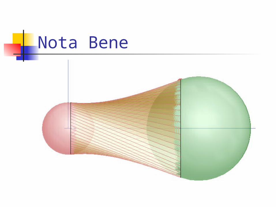
Nota Bene

L-pppp Solved
Coordinate system choice
),,,(:
),0,,(:
),0,0,(:
),0,0,0(:
),,;,,(:
44
33
22
11
rfedS
rcbS
raS
rS
wvuzyxL

Constraint Equations on L
1
0
)()()()(
)()()(
)()(
222
23
2222
22
2222
21
2222
20
222
wvu
zwyvxu
rfwevdufzeydx
rcvbuzcybx
rauzyax
rzyx

Algebraic Simplifications Use equations (2), (3) and (4) to
solve for x, y, and z Resulting system has three
equations of degree 4, 3, and 2 (Bezout bound 24)
But if (u,v,w) solves the system, then so does (-u,-v,-w)…

Structure of surface of line tangents to 3 spheres on Gauss sphere

L-Lppp Problem Construct a line from another line and
up to 3 points Subcases, by LL constraints:
L-Lpp: The lines are parallel; clearly 2 solutions maximum
L-Lpp: A distance is required; need good understanding of a kinematic curve
L-Lppp: No distance is required (includes perpendicular); intersect 3 of the L-Lpp curves

Subcase LL Parallel Take a plane perpendicular
to the fixed line Sphere silhouettes
intersect in up to two points
Up to two solutions

Main Tool Given 2 spheres and a direction,
find the two tangents in that direction

Subcase LL Distance Only 2 spheres needed Fix plane at complement angle to
fixed line Rotate the 2 spheres around the
fixed axis yielding silhouette intersection curves
Intersect with horizontal line

Silhouette curve degree 18?

No LL Distance Additional constraint from a third
sphere (point with distance) Intersect the silhouette
intersection pairs No degree estimates

Silhouette intersection curves meet at intersections of sought tangents


