Computer assignments ELG 4172, Winter 2009by Martin Bouchard

Assignment #1 : Steady state, transient and frequency response of discrete

time systems

a) For the following system :

y[n] + 0.9 y[n-2] = 0.3 x[n] + 0.6 x[n-1] + 0.3 x[n-2]

find what is the output signal when a step function of amplitude 3 is the input signal (i.e

x[n] = 3 u[n]). Assume initial rest conditions (y[-1]=0, y[-2]=0). Use a long enough

section of the input signal so that the output from the Matlab function filter is nearly

constant. Plot the output signal and find the steady state amplitude at the output of the

system as n becomes very large. Use the stem function to plot discrete time signals.

b) The variable part of the response in a) is called the transient response. Find the

transient response ( = total response - steady state response), and plot it for 0 n 50.

c) Verify that the response to a step of amplitude 15 is five times that found in part a).

Explain why this is the case.

d) Knowing that the impulse unit (Dirac) can be expressed by the difference between two

step signals ([n] = u[n] – u[n-1]), express the impulse response h[n] as a function of the

unit step response s[n]. Plot the impulse response h[n].

e) In the case of complex sinusoidal input signals of the form u[n], as the transient in

the output of the system will die away, the form of the output approaches G , where

G is a complex number. Note that G will vary with . For the same system as in a), plot

M. Bouchard, 20091

the real and imaginary parts of the response to the complex exponential x[n]= u[n]

(using filter, real and imag functions). Use a long enough section of the input section so

that the transient has died out. Find the steady state amplitude gain of the system for

the x[n] input signal.

f) Find the frequency response of the system, using the freqz function. Plot the amplitude

and phase of the frequency response. Check the gain for =0 and = . Compare with

your results from a) and e).

g) Using the fact that the system is linear and that it has a real impulse response (and a

complex conjugate symmetry in the transfer function), prove that if an input

produces an output , where G is a complex number, the input will

produce an output . Verify this by using the input signal and

compare the output with the gain found in f). Plot the input and output signals.

M. Bouchard, 20092

Assignment #2 : Filters and resonators

a) Find the frequency response of the discrete time systems described by the following

difference equations. Plot the frequency responses and state what type of filters each of

these equations describe.

y[n]+0.13y[n-1]+0.52y[n-2]+0.3y[n-3]=0.16x[n]-0.48x[n-1]+0.48x[n-2]-0.16x[n-3]

y[n]-0.268y[n-2]=0.634x[n]-0.634x[n-2]

y[n]+0.268y[n-2]=0.634x[n]+0.634x[n-2]

10y[n]-5y[n-1]+y[n-2]=x[n]-5x[n-1]+10x[n-2]

b) Consider the following system describing a resonator :

.

Provide an approximate relation between and the frequency of the resonant peak in

(in terms of the pole locations).

c) Write a script to show the magnitude of the frequency response of the system. Use

some values of r in the range 0.7 < r < 1.0, and for each value find the frequency

response using freqz. Use a constant value of . What happens to the magnitude of

the peak and to the bandwidth of the peak as r increases ?

d) Using the impz function, find and plot the impulse response of the resonator when r=1,

for a non-zero value of . What is the name of the resulting system ?

M. Bouchard, 20093

e) Prove analytically that the following system is a notch filter :

.

Plot the frequency response for and verify that it is a notch filter.

f) If this filter/system is used to eliminate a component at 60 Hz in a signal that was

sampled at 1000 Hz, what is the value required ? What will be the (approximate) gain

of the filter at the other frequencies ?

g) Generate a 60 Hz sinusoid samples at 1000 Hz sampling rate. Filter this signal by the

notch filter and verify that it eliminates the 60 Hz component. Plot the different signals.

M. Bouchard, 20094

Assignment #3 : Sampling, A/D conversion and D/A conversion

Since Matlab works on a digital system, we can only simulate the sampling of a

continuous signal to produce a discrete time signal (i.e. we must approximate the

continuous signal by a discrete time signal obtained with a high sampling rate). The same

comment applies for A/D conversion and D/A conversions. But visual and audio

representations of the aliasing are still possible.

1) Time domain representation of sampling and aliasing

a) sampled at a frequency of produces the discrete time signal

. Use a value of = 8 kHz. By varying the value of , it is

possible to illustrate the aliasing. For an interval of 10 ms, plot the sampled sine wave if

= 300 Hz, using stem. The phase can be arbitrary. You should see a sinusoidal

pattern. If not, use the plot function which creates the impression of a continuous function

from discrete time values.

b) Vary the frequency from 100 Hz to 475 Hz, in steps of 125 Hz. The apparent

frequency of the sinusoid should be increasing, as expected. Use subplot to put four plots

on one screen.

c) Vary the frequency from 7525 Hz to 7900 Hz, in steps of 125 Hz. Note that the

apparent frequency of the sinusoid is now decreasing. Explain why.

d) Vary the frequency from 32100 Hz to 32475 Hz, in steps of 125 Hz. Can you

predict in advance if the frequency will increase or decrease ? Why/How ?

2) Frequency domain representation of sampling and aliasing, A/D and D/A

convertions

M. Bouchard, 20095

e) Simulate a continuous sinusoid signal by generating samples separated by a small

interval of = 1/80000 second (time resolution):

, n=0,1,2,...

Plot as a continuous function 1000 samples of the resulting signal when the frequency

is 2 kHz.

f) Plot the continuous time Fourier transform (amplitude) of the signal using the

following function, where dt is the time resolution :

function freqmagplot(x,dt)L=length(x);Nfft=round(2.^round(log2(5*L)));X=fft(x,Nfft);f=((1/dt)/Nfft)*(0:1:Nfft/2-1);plot(f,abs(X(1:Nfft/2)));title('Magnitude of Fourier Transform');xlabel('Frequency'),grid;

This function simulates a discrete time or a continuous time Fourier Transform by

computing a DFT/FFT with a high resolution.

g) To simulate the A/D conversion at a rate of = 8000 Hz (sampling period of 1/8000

second), we need to keep one sample in every 10 samples from the signal in e). Plot the

resulting discrete time signal and its discrete time Fourier transform (again freqmagplot

can be used, but with the appropriate value for dt !).

h) To simulate the D/A conversion, we need to follow two steps. In the first step, the

discrete time signal from g) is converted to an analog pulse signal. An analog pulse signal

is the ideal case, in practice the analog signal is typically the output of a sample and hold

device. To simulate the analog pulse signal, 9 zeros are added between each sample of

the discrete time signal from g), so that the resulting simulated continuous signal has the

M. Bouchard, 20096

original resolution of 1/80000 sec. Plot the resulting signal and its continuous time

Fourier transform.

i) The second step of the D/A conversion is to filter (interpolate) the signal found in h), so

that the samples with zero values can be filled with non-zero values. In the frequency

domain, this means low-pass filtering the continuous Fourier transform found in h) so

that only the first peak remains. The resulting Fourier transform should be almost

identical to the transform found in f). To perform the low-pass filtering, use the following

filter coefficients

[b,a]=cheby2(9,60, *1/80000);

and the function filter. Plot the signal at the output if the filter, discard the first 200

samples (transient response) and plot the continuous time Fourier transform of the

resulting signal. Compare with f).

j) Repeat the steps in e) f) g) h) i) with = 2500 Hz, 3500 Hz, 4500 Hz, 5500 Hz (plots

not required here). When does aliasing occurs ? What is the effect of aliasing on the

output signal of the D/A converter (found in i) ) ?

M. Bouchard, 20097

Assignment #4 : Windowing

A window acts in the time domain by truncating the length of a signal :

y[n]=x[n] w[n], where w[n]=0 outside of 0 n L-1.

In the frequency domain, the effect of the windowing operation is :

. Therefore, the spectrum of y[n] is different from the

spectrum of x[n], and this difference should be minimized by the choice of a proper

window.

a) When only the values of x[n] in the interval 0 n L-1 are kept, but there is no

weighting function w[n] applied to x[n], then the window function w[n] is called

rectangular or uniform (i.e. w[n]=1 0 n L-1). This window can be generated by

boxcar in Matlab. Compute the DTFT of a rectangular window w[n] of length 21, using

freqmagplot with dt=1. Plot the magnitude on a dB scale or a linear scale.

b) Repeat for a length of 16, 31 and 61 coefficients. What is the effect of the window

length on the size of the mainlobe and on the amplitude of the sidelobes (relative to the

mainlobe amplitude)?

c) A triangular window (also called Bartlett window) can be generated using the triang

function. Generate the DTFT for triangular windows of length 31 and 61, and plot the

magnitude response in dB. Compare with the results from a) and b).

d) Since a triangular window can be seen as the convolution of two smaller rectangular

windows, explain the difference in mainlobe width for the rectangular and triangular

windows.

M. Bouchard, 20098

e) The Hamming, von Hann (Hanning) and Blackman windows can be generated in

Matlab using the hamming, hanning and blackman functions. Plot on the same graph the

Hamming, Hanning and Blackman windows for a length of 31. Plot on the same graph

the magnitude of the DTFT (again estimated by a DFT/FFT) of these windows, and the

DTFT of the rectangular window. Compare the width of the mainlobes and the amplitude

of the sidelobes. Zoom in the low-frequency part of the spectrum if you want to see more

clearly the mainlobes.

f) The Kaiser window (found using the kaiser function) is widely used for the design of

simple FIR filters. In the Kaiser window, there is a parameter that offers a trade-off

between the sidelobes height and the width of the mainlobe. A value between 0 and 10

should be used in practice. Generate three Kaiser windows of length 31. Try different

values of : 3, 5 and 8. Plot the coefficients on one graph. Compute the DTFTs of these

windows and plot the magnitude (in dB) on these windows on one graph. Comment on

the effect of and compare the Kaiser windows with the Hamming window.

g) An important notion in spectrum analysis is the notion of resolution. It is important to

understand that the spectral resolution caused by a windowing operation is totally

different from the spectral resolution of a DFT/FFT. The loss of resolution caused by

windowing directly affects the DTFT, and therefore it is not caused by the DFT/FFT

sampling of the DTFT. When a large size DFT/FFT is used (using zero padding), the

main factor that will limit the spectral resolution is the windowing operation, and not the

DFT/FFT operation. Generate 64 samples of the following signal, choosing distinct

values for and :

x[n]=cos( n)+cos( n + 0.4).

Using freqmagplot (see assignment # 2), compute the DTFT of x[n] and plot the

magnitude. Find how small can the difference between the angular frequencies and

be and still see two separate peaks in the DTFT. This difference is a rough estimate of

M. Bouchard, 20099

the resolution. As a starting point, you can choose values in the neighborhood of for

the difference in frequencies, where L is the window length.

h) Repeat g) for window lengths of 128 and 256 samples. What are the resulting

resolutions ?

i) For a window length of 128, find the resolution (as in g) ) of the Hanning, Hamming

and Blackman windows, using the same signal x[n]=cos( n)+cos( n + 0.4).

M. Bouchard, 200910

Assignment #5 : FIR filter design

Design with frequency sampling

a) Design a length-23 linear-phase FIR low-pass filter to approximate an ideal response

that has a passband edge of radians/sample. First, form a vector of samples of

the ideal amplitude response over frequencies from 0 to . This vector has ones in the

passband and zeros in the stopband. Use the following lines :

wo=0.3*pi;len= 23;pass_len=fix(wo*len/(2*pi))+1;Ad=[ones(1,pass_len),zeros(1,len-2*pass_len+1),ones(1,pass_len-1)];stem(Ad);

Next, form a vector of ideal phase response of the form . Use the following

lines :

M=(len-1)/2;k=[0:len-1];pd=exp(-2*pi*j*M*k/len);

The resulting desired sampled frequency response is simply : Hd=Ad.*pd. Using the

inverse FFT, find and plot the impulse response h[n] that will produce the sampled

frequency response. h[n] should be real and symetric. If h has a small imaginary

component that should be neglected, then just use h=real(h) to keep the real part. If the

imaginary component is not small, then you have made a mistake.

b) Now find the real (i.e. not sampled) frequency response of the filter, using freqz. Plot

the magnitude and compare with the ideal sampled magnitude Ad. Plot the phase of the

frequency response using angle and unwrap. Where do jumps occur in the phase

frequency response ?

c) Plot the location of the zeros on the complex z-plane with

M. Bouchard, 200911

plot(roots(h),’o’);

Explain the location of the zeros (in terms of linear phase and low-pass behavior).

d) Design a 23 coeffs. FIR filter as in a) but this time with a phase response of zero (i.e

pd=zeros(1,len) ). Find the resulting impulse response h[n], and the magnitude and phase

frequency response of this filter h[n]. Is h[n] symetrical/anti-symetrical ? How is the

magnitude response ? Is the phase response linear phase ? Why ?

e) Design a 23 coeffs. FIR filter as in a) but this time with value of a M=5. Find the

resulting impulse response h[n], and the magnitude and phase frequency response of this

filter h[n]. Is h[n] symetrical/anti-symetrical ? How is the magnitude response ? Is the

phase response linear phase ?

f) From a), d), and e), what is the effect of M and why should it be set to M=(len-1)/2 ?

g) Now design an even length filter of length 22, using the same approach as in a). Find

the resulting impulse response h[n], and the magnitude and phase frequency response of

this filter h[n]. Note that an symmetric even-length linear-phase FIR filter always have a

zero at . Compare the amount of overshoot near the band edge with the design for

len=23.

Design with window functions

h) Design a length-23 linear-phase FIR low-pass filter with a passband edge of

radians/sample using a window approach. Do not use a frequency sampling technique as

in a). Use the windowing approach with the following windows: rectangular, Hanning,

Hamming and Kaiser with . Find the frequency response of the resulting filters, and

compare with the filter found in a).

M. Bouchard, 200912

Design with Chebyshev optimization / Parks-McClellan method / Remez exchange

algorithm

i) Design a length-23 linear-phase FIR low-pass filter with a passband edge of

radians/sample and a stopband edge of radians/sample, using the remez

Matlab function (you can also use the remezord function). What is the particular

characteristic of the magnitude of the filter frequency response ? How does the

frequency response compare with the responses from b) and h) ?

Modulation of filters

j) Transform one of the low-pass filters that you have designed in this assignment to a

band-pass filter. Hint : use the frequency shifting property or the modulation property of

the Fourier transform.

M. Bouchard, 200913

Assignment #6 : IIR filter design

Direct design of discrete time IIR filters using Matlab

a) Design a fifth-order digital Butterworth low-pass filter with a sampling frequency of

200 Hz and a passband edge of 60 Hz. Use the butter function. Plot the phase and

magnitude frequency response using freqz. Find the zeros and the poles, and plot them on

the same z-plane (using plot(roots(a),’x’) and plot(roots(b),’o’). Plot the significant

(energetic) part of the impulse response of the filter, using impz.

b) Repeat a) but use a Chebyshev type I filter with a passband ripple of 0.5 dB. Use the

cheby1 function. Compare with the plots found in a).

c) Repeat a) but use a Chebyshev type 2 filter with stopband edge of 65 Hz and a

stopband ripple 30 dB less than the passband. Use the cheby2 function. Compare with the

plots found in a).

d) Repeat a) but use an elliptic (Cauer) filter with a passband ripple of 0.5 dB and a

stopband ripple 30 dB less than the passband. Use the ellip function. Compare with the

plots found in a).

e) Matlab provides functions to estimate the order required for different types of IIR

filters in order to meet some specifications. For the following specifications :

sampling rate 200 Hz

passband ripple 0.1 dB

passband edge 28 Hz

stopband edge 32 Hz

stopband ripple below 30 dB

find the order required for Butterwoth, Chebyshev type 1, Chebyshev type 2 and elliptic

filters. Use the butterord, cheb1ord, cheb2ord, and elliord functions. Looking at the

M. Bouchard, 200914

magnitude of the frequency responses found in a) b) c) and d), explain intuitively why the

elliptic filter always have the lowest order (low order as a compromise of ...).

f) For the specifications in e), design a FIR Chebyshev/Parks-McClellan/Remez low-pass

filter, using remez and remezord functions. Verify the frequency response of the designed

filter. Compare the required order for this FIR filter with the orders of the IIR filters

found in e).Discuss.

Bilinear transform

g) It is desired to design a digital low-pass 4th order Butterworth filter with a sampling

frequency of 40 kHz and a passband edge of 8 kHz, using an analog filter and the bilinear

transformation. Find the required discrete time passband edge frequency. Then find the

prewarped analog passband edge that is required if the bilinear transformation is going to

be applied to the analog filter.

h) Design the low-pass analog 4th order Butterworth filter using the passband edge found

in g) and the function butter(N,Wn,'s'). Verify the frequency response and stability (via

the impulse response), using the freqs and impulse(b,a,Tf) functions for analog systems.

i) Using the [b2,a2] = bilinear(b,a,Fs) command, transform the continuous time filter to

a discrete time filter. Check the frequency response of the digital filter. Does it meet the

specifications ? Design an equivalent filter directly in the discrete time domain using

butter, and compare the results.

Design of filters by frequency transformation

j) It is possible to directly design a digital IIR highpass, bandpass or band reject filter

using the butter, cheby1, cheby2 and ellip functions. Design a 5th order Chebyshev type I

bandpass filter with a sampling frequency of 20 Hz, a lower passband edge of 5 Hz, an

upper passband edge of 8 Hz, and a passband ripple of 1 dB. Plot the frequency response

and the impulse response.

M. Bouchard, 200915

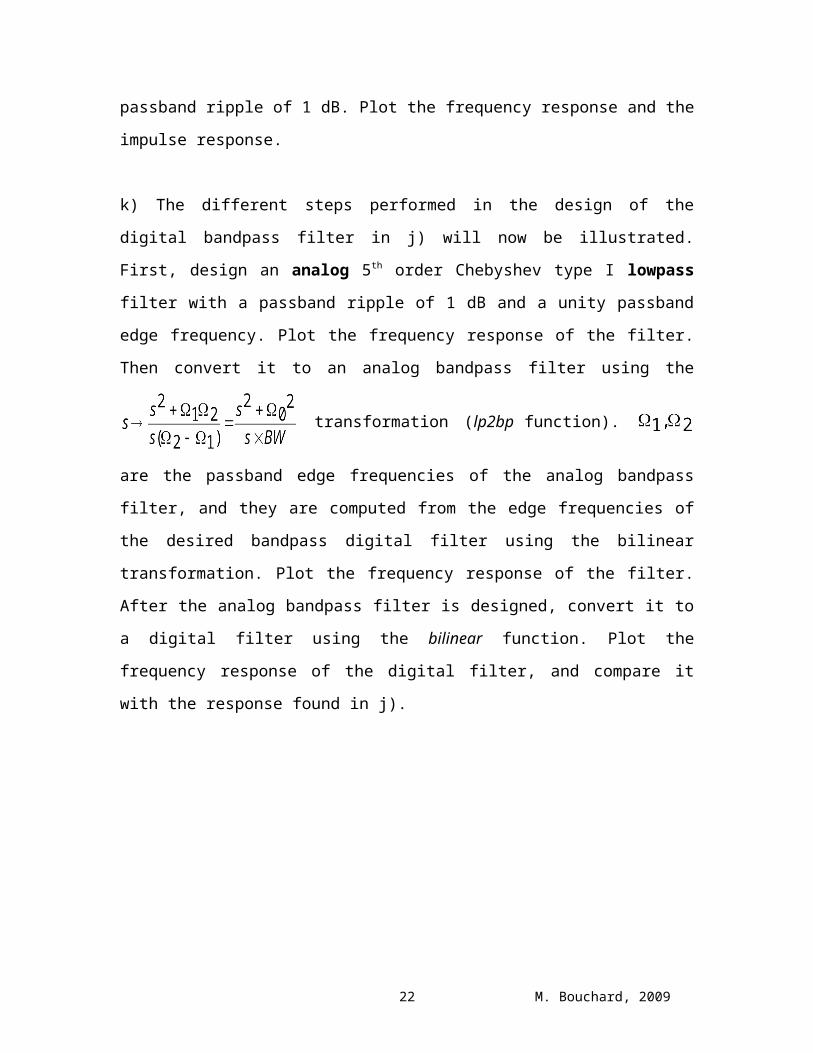
k) The different steps performed in the design of the digital bandpass filter in j) will now

be illustrated. First, design an analog 5th order Chebyshev type I lowpass filter with a

passband ripple of 1 dB and a unity passband edge frequency. Plot the frequency

response of the filter. Then convert it to an analog bandpass filter using the

transformation (lp2bp function). are the passband edge

frequencies of the analog bandpass filter, and they are computed from the edge

frequencies of the desired bandpass digital filter using the bilinear transformation. Plot

the frequency response of the filter. After the analog bandpass filter is designed, convert

it to a digital filter using the bilinear function. Plot the frequency response of the digital

filter, and compare it with the response found in j).

M. Bouchard, 200916

Assignment #7 : Finite Word Effects

A common model for the quantization of signals is the following model :

vq[n] = v[n] + e[n]

where v[n] is the un-quantized discrete time signal

e[n] is the quantization error

vq[n] is the quantized discrete time signal.

a) Generate an input signal v[n] from –0.7 to 0.7 using a step size of . Using a small

step size will simulate in Matlab the continuous amplitude of a non-quantized signal.

Generate a quantized version vq[n], using the function fixedpointquant :

function X = fixedpointquant( s, bit, rmode, lmode )%fixedpointquant simulated fixed-point quantization%-------% Usage: X = fixedpointquant( S, BIT, RMODE, LMODE )%% returns the input signal S reduced to a word-length% of BIT bits and limited to the range [-1,1). The type of% word-length reduction and limitation may be chosen with% RMODE: 'round' rounding to nearest level% 'trunc' 2's complement truncation% LMODE: 'sat' saturation limiter% 'overfl' 2's complement overflowif nargin ~= 4; error('usage: fxquant( S, BIT, RMODE, LMODE ).');end;if bit <= 0 | abs(rem(bit,1)) > eps; error('wordlength must be positive integer.');end;Plus1 = 2^(bit-1);X = s * Plus1;if strcmp(rmode, 'round'); X = round(X);elseif strcmp(rmode, 'trunc'); X = floor(X);else error('unknown wordlength reduction spec.');end;if strcmp(lmode, 'sat');

M. Bouchard, 200917

X = min(Plus1 - 1,X); X = max(-Plus1,X);elseif strcmp(lmode, 'overfl'); X = X + Plus1 * ( 1 - 2*floor((min(min(X),0))/2/Plus1) ); X = rem(X,2*Plus1) - Plus1;else error('unknown limiter spec.');end;X = X / Plus1;

This function simulates the fixed point quantization in the interval [-1.0 1.0] of a non-

quantized signal. Use a wordlength of 3 bits with the function, with a rounding and a

saturation for the quantizer. Compute e[n]=vq[n]-v[n], and plot vq[n] versus v[n], and

e[n] versus v[n]. What are the statistical properties of the error e[n] (mean, max.,

distribution) ?

b) Generate a Gaussion random input signal with zero mean and variance S of 0.01, using

randn with 10000 samples. Quantize the signal using fixedpointquant, with various word

length (number of bits). Find the S/N ratio in dB (energy of v[n] / energy of e[n]) for each

wordlength, and find the improvement in the S/N ratio provided by an additional bit.

c) For small values of variance S and a fixed number of bits, the S/N ratio will linearly

increase with S (because the variance of the quantization noise is constant). However, for

large values of the variance S (S=0.5 for example), the S/N ratio will not increase with an

increase in S. What happens in this case ? Hint : check the e[n] and vq[n] signals.

d) Repeat a) by using a 2's complement truncation quantizer instead of a rounding

quantizer. Compare the mean, the maximum and the distribution of the error signal e[n]

with the one found in a).

e) Finite word effects also affect the performance of digital filters. All filter structures

have the same input-output behavior when unlimited wordlength is used, but this is not

the case in practice, and some structures produce much better results in finite word

environments. For fixed point implementations of filters, the coefficients must have a

quantized amplitude in the [-1.0 1.0] interval. Therefore, after a design step the

M. Bouchard, 200918

coefficients have to be scaled to fit in this interval. This will affect the gain of the filter,

and therefore an inverse scaling is required at the output of the filter. The coefficients can

be scaled using the function quantizecoeffs :

function [aq,nfa] = quantizecoeffs(a,w);f=log(max(abs(a)))/log(2); % normalisation by n, a power of 2, so that all coeffs n=2^ceil(f); % are in the interval [-1 1]an=a/n;aq= fixedpointquant(an,w,’round’,’sat’);nfa=n;

Using the FIR half-band low-pass filter obtained with b=remez(30,[0 0.4 0.6 1], [1 1 0

0]), compute the frequency response of the un-quantized coefficients using freqz.

f) Quantize the coefficients from e) using quantizecoeffs with 6, 10, 16 bits wordlengths.

Compare the frequency response of the quantized filter in the passband and the stopband

with the frequency response of the un-quantized filter.

g) Does the quantization of the coefficients in the direct form structure destroy the linear

phase property of FIR linear phase un-quantized filters ? Why ?

h) Plot using freqz the frequency response of the IIR low-pass elliptic filter obtained with

[b,a]=ellip(7, 0.1, 40, 0.4).

i) Quantize the coefficients of the IIR filter using the quantizecoeffs function, with 6, 10

and 16 bits wordlengths. Plot the frequency response in each case. What do you observe ?

Explain.

j) Coefficients of the cascade form can be found using the following instructions :

[b,a]=ellip(7, 0.1, 40, 0.4) % direct form [Z,p,k] = TF2ZP(b,a); % zero-pole formsos=ZP2SOS(Z,p,k); % cascade form

M. Bouchard, 200919

Each row of the matrix sos contains 6 elements. The first 3 elements are the coefficients

of the numerator in a second order section of a cascade system, while the last 3 elements

are the denominator coefficients. Compute the frequency response of each section using

freqz, and find the global frequency response of the system. Verify that it is the same as

in h). Hint : to combine the frequency response of the sections, you can use the following

approach :

h=zeros(1000,N);g=ones(1000,1);for(i=1:1:N)

[h(:,i),w]=freqz(sos(i,1:3), sos(i,4:6),1000);g(:,1)=g(:,1).*h(:,i);

end

k) Quantize the coefficients of each section of the cascade structure using quantizecoeffs

with 6, 10, 16 bits wordlengths. Compute the frequency response of each section using

freqz, and find the global frequency response of the system. Compare your results with

the results from i).

M. Bouchard, 200920

Assignment #8 : Decimation/Interpolation/Multirate Signal Processing

Change of sampling rate

a) It is desired to decrease the sampling rate of the signal , by a factor

of 2/3, using interpolation and decimation techniques. Which operation should be

performed first : interpolation by 2 or decimation by 3 ? Does it matter ? Perform the

required interpolation and decimation (not necessarily in that order). Plot the time domain

signals and their Fourier transform at the various steps of the interpolation/decimation

process.

Frequency zoom

b) In some cases, the size of a FFT that can be computed is limited by speed of execution

or by memory size. Many spectrum analyzers can only perform FFTs with 1024 samples

or less. This reduces the resolution of the FFT (i.e the sampling of the spectrum), which

is the sampling rate divided by the FFT size. Note that the resolution is also affected by

the window operation, as seen in assignment #4. To improve the FFT resolution, it is

possible to “zoom” on a section of the spectrum, thus obtaining N samples in this section

by using the FFT. This requires the use of filtering and decimation techniques. First, load

in Matlab memory some sound signal from any WAV file, using wavread. Keep the first

2050 samples of the read data. Perform a FFT on the last 2000 samples of the 2050

samples and plot the magnitude of the FFT values. Note that the values produced by the

FFT cover the [0, ] range, so the high frequencies are the middle values.

c) Now suppose that the maximum size of FFT that can be used is N=1000, but the same

resolution is required as in d), where N=2000 was used. This can be done for different

parts of the spectrum, by filtering and decimation. Let’s consider the case of the high

frequencies ( [ , ] interval). Design a half-band highpass FIR filter with a length of

50. Filter the 2050 samples by the FIR filter, and keep the 2000 last values of the output

samples. Multiply the resulting signal by . Decimate the resulting signal by a factor

of 2, thus keeping only 1000 values. Perform the FFT of those values, and plot the

M. Bouchard, 200921

magnitude of the FFT values. Compare with the middle (high frequencies) FFT values

found in d). You should get similar values and similar resolutions. Explain analytically

(with graphs) the process that was performed. The same process could also be applied to

zoom low frequency values. In fact, if the spectrum is divided in D parts, with D integer,

a zoom can be performed on any part using filtering, modulation and decimation.

M. Bouchard, 200922