Elias Bareinboim* and Judea Pearl A General Algorithm...

Elias Bareinboim* and Judea Pearl

A General Algorithm for Deciding Transportability ofExperimental Results

Abstract: Generalizing empirical findings to new environments, settings, or populations is essential in mostscientific explorations. This article treats a particular problem of generalizability, called “transportability”,defined as a license to transfer information learned in experimental studies to a different population, onwhich only observational studies can be conducted. Given a set of assumptions concerning commonalitiesand differences between the two populations, Pearl and Bareinboim [1] derived sufficient conditions thatpermit such transfer to take place. This article summarizes their findings and supplements them with aneffective procedure for deciding when and how transportability is feasible. It establishes a necessary andsufficient condition for deciding when causal effects in the target population are estimable from both thestatistical information available and the causal information transferred from the experiments. The articlefurther provides a complete algorithm for computing the transport formula, that is, a way of combiningobservational and experimental information to synthesize bias-free estimate of the desired causal relation.Finally, the article examines the differences between transportability and other variants of generalizability.

Keywords: causal effects, experimental findings, generalizability, transportability, external validity

*Corresponding author: Elias Bareinboim, Department of Computer Science, University of California, Los Angeles, CA, USA,E-mail: [email protected] Pearl, Department of Computer Science, University of California, Los Angeles, CA, USA, E-mail: [email protected]

1 Introduction

The problem of transporting knowledge from one population to another is pervasive in science. Conclusionsthat are obtained in a laboratory setting are transported and applied elsewhere, in an environment thatdiffers in many aspects from that of the laboratory. Experiments conducted on a group of subjects areintended to inform policies on a different group, usually more general and in which the studied group is justone of its parts.

Surprisingly, the conditions under which this extrapolation can be legitimized were not formallyarticulated until very recently [1–3]. Although the problem has been discussed in many areas of statistics,economics, and the health sciences, under rubrics such as “external validity” [4, 5], “meta-analysis” [6–8],“overgeneralization” [9], “quasi experiments” [10, 11 (Ch. 3)], “heterogeneity” [12], these discussions arelimited to verbal narratives in the form of heuristic guidelines for experimental researchers – no formaltreatment of the problem has been attempted to answer the practical problem of generalizing acrosspopulations posed in this article. (See Section 6 for related work.)

Recent developments in causal inference enable us to tackle this problem formally. First, the distinctionbetween statistical and causal knowledge has received syntactic representation through causal diagrams[13–16]. Second, graphical models provide a language for representing differences and commonalitiesamong domains, environments, and populations [1]. Finally, the inferential machinery provided by thedo-calculus [13, 16, 17] is particularly suitable for combining these two advances into a coherent frameworkand developing effective algorithms for knowledge transfer.

Armed with these tools, we consider transferring causal knowledge between two populations � and ��.In population �, experiments can be performed and causal knowledge gathered. In ��, potentially differentfrom �, only passive observations can be collected but no experiments conducted. The problem is to infer a

doi 10.1515/jci-2012-0004 Journal of Causal Inference 2013; 1(1): 107–134

Brought to you by | University of California - Los Angeles - UCLA LibraryAuthenticated | 131.179.232.118Download Date | 8/9/13 12:34 AM

TECHNICAL REPORT R-404

May 2013

causal relationship R in �� using knowledge obtained in �. Clearly, if nothing is known about therelationship between � and ��, the problem is trivial; no transfer can be justified. Yet the fact that allexperiments are conducted with the intent of being used elsewhere (e.g., outside the laboratory) implies thatscientific explorations are driven by the assumption that certain populations share common characteristicsand that, owed to these commonalities, causal claims would be valid in new settings even where experi-ments cannot be conducted.

To formally articulate commonalities and differences between populations, a graphical representationnamed selection diagrams was devised in [1], which represent differences in the form of unobserved factorscapable of causing such differences. Given an arbitrary selection diagram, our challenge is to decidewhether commonalities override differences to permit the transfer of information across the two popula-tions. We show that this challenge can be met by an effective procedure that decides when and howtransportability is feasible.

The article is organized as follows. In section 2, we motivate the problem of transportability using threesimple examples and informally summarize the findings of Pearl and Bareinboim [1]. In section 3, weformally define the notion of selection diagrams and transportability, exemplify how it can be reduced to aproblem of symbolic transformation in do-calculus, and provide examples for models that prohibit trans-portability. In section 4, we provide a graphical criterion for deciding transportability in arbitrary diagrams.In section 5, we provide an effective procedure for deciding transportability, which returns a correcttransport formula whenever such exists. In section 6, we compare transportability to other problems ofgeneralizing empirical findings. Section 7 provides concluding remarks.

2 Motivation

To motivate the formal treatment of transportability, we use three simple examples taken from [1] andgraphically depicted in Figure 1.

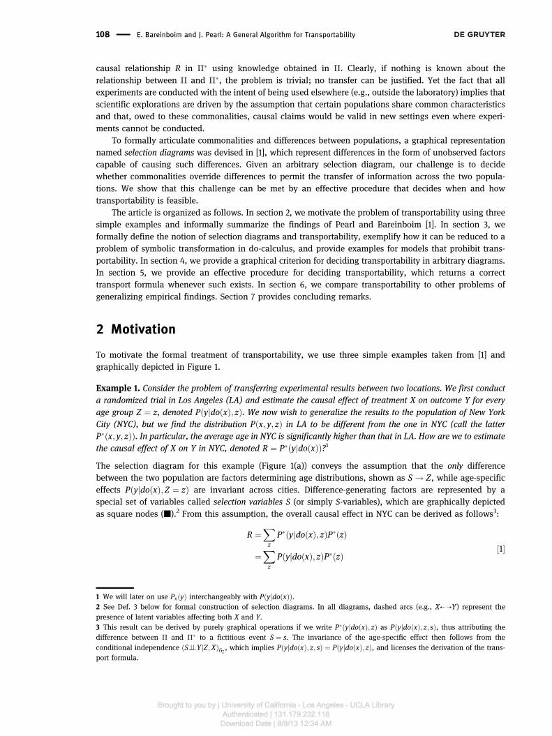
Example 1. Consider the problem of transferring experimental results between two locations. We first conducta randomized trial in Los Angeles (LA) and estimate the causal effect of treatment X on outcome Y for everyage group Z ¼ z, denoted PðyjdoðxÞ; zÞ. We now wish to generalize the results to the population of New YorkCity (NYC), but we find the distribution Pðx; y; zÞ in LA to be different from the one in NYC (call the latterP�ðx; y; zÞÞ. In particular, the average age in NYC is significantly higher than that in LA. How are we to estimatethe causal effect of X on Y in NYC, denoted R ¼ P�ðyjdoðxÞÞ?1

The selection diagram for this example (Figure 1(a)) conveys the assumption that the only differencebetween the two population are factors determining age distributions, shown as S! Z, while age-specificeffects PðyjdoðxÞ; Z ¼ zÞ are invariant across cities. Difference-generating factors are represented by aspecial set of variables called selection variables S (or simply S-variables), which are graphically depictedas square nodes (■).2 From this assumption, the overall causal effect in NYC can be derived as follows3:

R ¼Xz

P�ðyjdoðxÞ; zÞP�ðzÞ

¼Xz

PðyjdoðxÞ; zÞP�ðzÞ½1�

1 We will later on use PxðyÞ interchangeably with PðyjdoðxÞÞ.2 See Def. 3 below for formal construction of selection diagrams. In all diagrams, dashed arcs (e.g., X⇠⇢Y) represent thepresence of latent variables affecting both X and Y.3 This result can be derived by purely graphical operations if we write P�ðyjdoðxÞ; zÞ as PðyjdoðxÞ; z; sÞ, thus attributing thedifference between � and �� to a fictitious event S ¼ s. The invariance of the age-specific effect then follows from theconditional independence ðS\\YjZ;XÞGx

, which implies PðyjdoðxÞ; z; sÞ ¼ PðyjdoðxÞ; zÞ, and licenses the derivation of the trans-port formula.

108 E. Bareinboim and J. Pearl: A General Algorithm for Transportability


The last line constitutes a transport formula for R. It combines experimental results obtained in LA,PðyjdoðxÞ; zÞ, with observational aspects of NYC population, P�ðzÞ, to obtain an experimental claimP�ðyjdoðxÞÞ about NYC.4

Our first task in this article will be to explicate the assumptions that renders this extrapolation valid. Weask, for example, what must we assume about other confounding variables beside age, both latent andobserved, for eq. [1] to be valid, or, would the same transport formula hold if Z was not age, but some proxyfor age, say, “language skills” (Figure 1(b)). More intricate yet, what if Z stood for an exposure-dependentvariable, say hyper-tension level, that stands between X and Y (Figure 1(c))?

Let us examine the proxy issue first.

Example 2. Let the variable Z in Example 1 stand for subjects’ language skills, and let us assume that Z doesnot affect exposure ðXÞ or outcome ðYÞ, yet it correlates with both, being a proxy for age which is not measuredin either study (see Figure 1(b)). Given the observed disparity PðzÞ�P�ðzÞ, how are we to estimate the causaleffect P�ðyjdoðxÞÞ for the target population of NYC from the z-specific causal effect PðyjdoðxÞ; zÞ estimated atthe study population of LA?

Our intuition dictates, and correctly so, that since reading ability has no causal effect on treatment nor onthe outcome the proper transport formula would be

P�ðyjdoðxÞÞ ¼ PðyjdoðxÞÞ ½2�

namely, the causal effect is “directly” transportable with no calibration needed (to be shown later on). Thiswill be the case even if the observed joint distribution P�ðx; y; zÞ is the same as in Example 1 where Z standsfor age. We see, therefore, that the proper transport formula depends on the causal context in whichpopulation differences are embedded, not merely on the joint distribution over the observed variables.

This example also demonstrates why the invariance of Z-specific causal effects should not be taken forgranted. While justified in Example 1, with Z ¼ age, it fails in Example 2, in which Z was equated with“language skills.” The intuition is clear. A NYC person at skill level Z ¼ z is likely to be in a totally differentage group from his skill-equals in LA and, since it is age, not skill that shapes the way individuals respondto treatment, it is only reasonable that LA residents would respond differently to treatment than their NYCcounterparts at the very same skill level.

Example 3. Examine the case where Z is a X-dependent variable, say a disease bio-marker, standing on thecausal pathways between X and Y as shown in Figure 1(c). Assume further that the disparity PðzÞ�P�ðzÞ is

S

Z

Z

S

YXYX

S

Z YX

(c)(b)(a)

Figure 1 Causal diagrams depicting Examples 1–3. In (a) Z represents “age.” In (b) Z represents “linguistic skills” while age (inhollow circle) is unmeasured. In (c) Z represents a biological marker situated between the treatment (X) and a disease (Y).

4 Eq. [1] reflects the familiar method of “standardization” – a statistical extrapolation method that can be traced back to acentury-old tradition in demography and political arithmetic [18–21]. We will show that standardization is only valid undercertain conditions.

E. Bareinboim and J. Pearl: A General Algorithm for Transportability 109


discovered in each level of X and that, again, both the average and the z-specific causal effect PðyjdoðxÞ; zÞ areestimated in the LA experiment, for all levels of X and Z. Can we, based on the information given, estimate theaverage (or z-specific) causal effect in the target population of NYC?

Assuming that the disparity in PðzÞ stems only from a difference in subjects’ susceptibility to X, as encodedin the selection the diagram of Figure 1(c), we will demonstrate in section 3 that the correct transportformula should be

P�ðyjdoðxÞÞ ¼Xz

PðyjdoðxÞ; zÞP�ðzjxÞ; ½3�

which is different from both eqs. [1] and [2]. It calls instead for the z-specific effects to be weighted by theconditional probability P�ðzjxÞ, estimated at the target population.

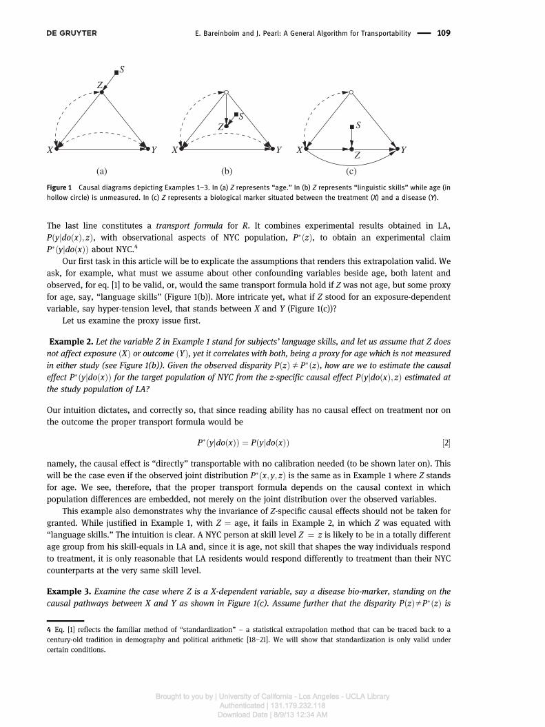
In these three intuitive examples transportability amounts to simple operations (i.e., recalibration, directtransport, and weighted recalibration); however, in more elaborate examples, the full power of formalanalysis would be required. For instance, Pearl and Bareinboim [1] showed that, in the problem depicted inFigure 2, where both the Z-determining mechanism and the U-determining mechanism are suspect of beingdifferent, the transport formula for the relation P�ðyjdoðxÞÞ is given by

Xz

PðyjdoðxÞ; zÞXw

P�ðzjwÞXt

PðwjdoðxÞ; tÞP�ðtÞ

This formula instructs us to estimate PðyjdoðxÞ; zÞ and PðwjdoðxÞ; tÞ in the experimental population, thencombine them with the estimates of P�ðzjwÞ and P�ðtÞ in the target population. Pearl and Bareinboim [1]derived this formula using the following lemma, which translates the property of transportability to theexistence of a syntactic reduction using a sequence of do-calculus rules.

Lemma 1 [1]. LetDbe theselectiondiagramcharacterizing � and ��, and S a set of selection variables in D. Therelation R ¼ P�ðyjdoðxÞ; zÞ is transportable from � to �� if the expression PðyjdoðxÞ; z; sÞ is reducible, using therules of do-calculus, to an expression in which S appears only as a conditioning variable in do-free terms.

The logic of this reduction is simple. Terms lacking an S variable are estimable at the source populationwhile those lacking the do-operator are estimable non-experimentally at the target population. If such areduction exists, the resulting expression gives the transport formula for R.

Lemma 1 is declarative but not computationally effective, for it does not specify the sequence of rules leadingto the needed reduction, nor does it tell us if such a sequence exists. It is useful primarily as a verification tool, toconfirm the transportability of a given relation once we are in possession of a “witness” sequence.

S

S

ZW YX

V

T

U

Figure 2 Selection diagram with two “difference-producing” factors (S and S0); the derivation of transportability is moreinvolved using Lemma 1, and it is shown step by step using the algorithm in section 5.



To overcome this deficiency, Pearl and Bareinboim [1] proposed a recursive procedure (theirTheorem 3), which can handle many cases, among them Figure 2, but is not “complete”, that is, diagramsexist that support transportability and which the recursive procedure fails to recognize as such. Theprocedure developed in this article are guaranteed to make correct identification in all cases. We summarizeour contributions as follows:

● We derive a general graphical condition for deciding transportability of causal effects. We show thattransportability is feasible if and only if a certain graph structure does not appear as an edge subgraph ofthe inputted selection diagram.

● We provide necessary or sufficient graphical conditions for special cases of transportability, for instance,controlled direct effects (CDE).

● We construct a complete algorithm for deciding transportability of joint causal effects and returning aproper transport formula whenever those effects are transportable.

3 Preliminaries

The semantical framework in our analysis rests on structural causal models (SCM) as defined next, alsocalled probabilistic causal models or data-generating models.

Definition 1 (Structural Causal Model [22, p. 203]). A SCM is a 4-tuple M ¼ hU;V ; F;Pi where:

1. U is a set of background or exogenous variables, representing factors outside the model, which neverthelessaffect relationships within the model.

2. V is a set of endogenous variables fV1; :::;Vng, assumed to be observable. Each of these variables isfunctionally dependent on some subset PAi of U ¨VnfVig.

3. F is a set of functions ff1; :::; fng such that each fi determines the value of Vi 2 V, vi ¼ fiðpai; uÞ.4. A joint probability distribution PðuÞ over U.

In the structural causal framework [22, Ch. 7], actions are modifications of functional relationships,and each action doðxÞ on a causal model M produces a new model Mx ¼ hU;V; Fx;PðUÞi, where Fxis obtained after replacing fX 2 F for every X 2 X with a new function that outputs a constant value xgiven by doðxÞ. See Appendix 1 for a gentle introduction to structural models, or [23] for a more detaileddiscussion.

We follow the conventions given in [22]. We will denote variables by capital letters and their valuesby small letters. Similarly, sets of variables will be denoted by bold capital letters, sets of values bybold letters. We will use the typical graph-theoretic terminology with the corresponding abbreviationsPaðYÞG, AnðYÞG, and DeðYÞG, which will denote respectively the set of observable parents, ancestors,and descendants of the node set Y in G. By convention, these sets will include the arguments as well,for instance, the ancestral set AnðYÞG will include Y. We will usually omit the graph subscript wheneverthe graph in question is assumed or obvious. A graph GY will denote the induced subgraph Gcontaining nodes in Y and all arrows between such nodes. Finally, GXZ stands for the edge subgraphof G where all incoming arrows into X and all outgoing arrows from Z are removed.

Key to the analysis of transportability is the notion of “identifiability,” defined below, which expressesthe requirement that causal effects be computable from a combination of data P and assumptions embodiedin a causal graph G.

Definition 2 (Causal Effects Identifiability [22, p. 77]). The causal effect of an action doðxÞ on a set ofvariables Y such that Y ˙ X ¼ � is said to be identifiable from P in G if PxðyÞ is uniquely computable fromPðVÞ in any model that induces G.



Causal models and their induced graphs are normally associated with one particular domain (alsocalled setting, study, population, environment). In the transportability case, we extend this representationto capture properties of several domains simultaneously. This is made possible if we assume that there areno structural changes between the domains, that is, all structural equations share the same set ofarguments, though the functional forms of the equations may vary arbitrarily.5,6

Definition 3 (Selection Diagram). Let hM;M�i be a pair of SCM relative to domains h�;��i, sharing a causaldiagram G. hM;M�i is said to induce a selection diagram D if D is constructed as follows:

1. Every edge in G is also an edge in D;2. D contains an extra edge Si ! Vi whenever there might exist a discrepancy fi � f �i or PðUiÞ � P�ðUiÞ between

M and M�.

In words, the S-variables locate the mechanisms where structural discrepancies between the two domainsare suspected to take place.7 Alternatively, one can see a selection diagram as a carrier of invariance claimsbetween the mechanisms of both domains – the absence of a selection node pointing to a variablerepresents the assumption that the mechanism responsible for assigning value to that variable is thesame in the two domains.8

Armed with a selection diagram and the concept of identifiability, transportability of causal effects (ortransportability, for short) can be defined as follows:

Definition 4 (Causal Effects Transportability). Let D be a selection diagram relative to domains h�;��i. LethP; Ii be the pair of observational and interventional distributions of �, and P� be the observational distribu-tion of ��. The causal effect R ¼ P�xðyÞ is said to be transportable from � to �� in D if P�xðyÞ is uniquelycomputable from P;P�; I in any model that induces D.

In some broad sense, one can view transportability as a special case of identifiability, where the pair ofstructures constitutes a global model, and the task is to infer a property of one population from sum total ofthe information available (i.e., hP; I;P�i). However, the unique challenges of dealing with two diverseenvironments under two different experimental regimes, and the special problems that emerge from thiscombination can benefit appreciably from viewing transportability as distinct major extension of identifia-bility. To witness, all identifiable causal relations in ðG�;P�Þ are also transportable, because they can becomputed directly from �� and require no experimental information from �. This observation engender thefollowing definition of trivial transportability.

Definition 5 (Trivial Transportability). A causal relation R is said to be trivially transportable from � to ��, ifRð��Þ is identifiable from ðG�;P�Þ.

The following observation establishes another connection between identifiability and transportability. For agiven causal diagram G, one can produce a selection diagram D such that identifiability in G is equivalent totransportability in D. First set D ¼ G, and then add selection nodes pointing to all variables in D, which

5 This definition was left implicit in [1].6 The assumption that there are no structural changes between domains can be relaxed as follows. Starting with the structure inthe target population G�, make D ¼ G�, and then add S-nodes to D following the same procedure as in Def. 3.7 Transportability analysis assumes that enough structural knowledge about both domains is known in order to substantiate theproduction of their respective causal diagrams. In the absence of such knowledge, causal discovery algorithms might be used tohelp in inferring the diagrams from data [15, 22, 24].8 These invariance assumptions are analogous to the missing-arrows in the causal graphs [25] which allow one to identifycausal-effects from observational data.



represents that the target domain does not share any commonality with its pair – this is equivalent to theproblem of identifiability because the only way to achieve transportability is to identify R from scratch in thetarget domain.

Another special case of transportability occurs when a causal relation has identical form in bothdomains – no recalibration is needed. This is captured by the following definition.

Definition 6 (Direct Transportability). A causal relation R is said to be directly transportable from � to ��, ifRð��Þ ¼ Rð�Þ.

A graphical test for direct transportability of R ¼ P�ðyjdoðxÞ; zÞ follows from do-calculus and reads:ðS\\Y jX; ZÞG

X; in words, X blocks all paths from S to Y once we remove all arrows pointing to X and

condition on Z. As a concrete example, the z-specific effect in Figure 1(a) is the same in both domains;hence, it is directly transportable. Also, the effect P�ðyjdoðxÞÞ in Figure 1(b) is the same in both domains;hence, it is directly transportable.

These two cases will act as a basis to decompose the problem of transportability into smaller and moremanageable subproblems. For instance, let us estimate the effect R ¼ P�ðyjdoðxÞÞ in the bio-marker exampledepicted in Figure 1(c).

P�ðyjdoðxÞÞ ¼Xz

P�ðyjdoðxÞ; zÞP�ðzjdoðxÞÞ ½4�

¼Xz

P�ðyjdoðxÞ; zÞP�ðzjxÞ ½5�

¼Xz

PðyjdoðxÞ; zÞP�ðzjxÞ; ½6�

In eq. [4], the target relation R is conditioned on Z. The effect P�ðzjdoðxÞÞ in eq. [5] is trivially transportablesince it is identifiable in ��, and P�ðyjdoðxÞ; zÞ in eq. [6] is directly transportable since ðS\\Y jX; ZÞGx

.Now we turn our attention to conditions that preclude identifiability. The following lemma provides an

auxiliary tool to prove non-transportability and is based on refuting the uniqueness property required byDefinition 4.

Lemma 2. Let X;Y be two sets of disjoint variables, in population � and ��, and let D be the selectiondiagram. P�xðyÞ is not transportable from � to �� if there exist two causal models M1 and M2 compatible with Dsuch that P1ðVÞ ¼ P2ðVÞ, P�1 ðVÞ ¼ P�2 ðVÞ, P1ðVnWjdoðWÞÞ ¼ P2ðVnWjdoðWÞÞ, for any set W, all families havepositive distribution, and P�1 ðyjdoðxÞÞ�P�2 ðyjdoðxÞÞ.

Proof. Let I be the set of interventional distributions PðVnWjdoðWÞÞ, for any set W. The latter inequalityrules out the existence of a function from P;P�; I to P�xðyÞ. ■

While the problems of identifiability and transportability are related, Lemma 2 indicates that proofs of non-transportability are more involved than those of non-identifiability. Indeed, to prove non-transportabilityrequires the construction of two models agreeing on hP; I;P�i, while non-identifiability requires the twomodels to agree solely on the observational distribution P.

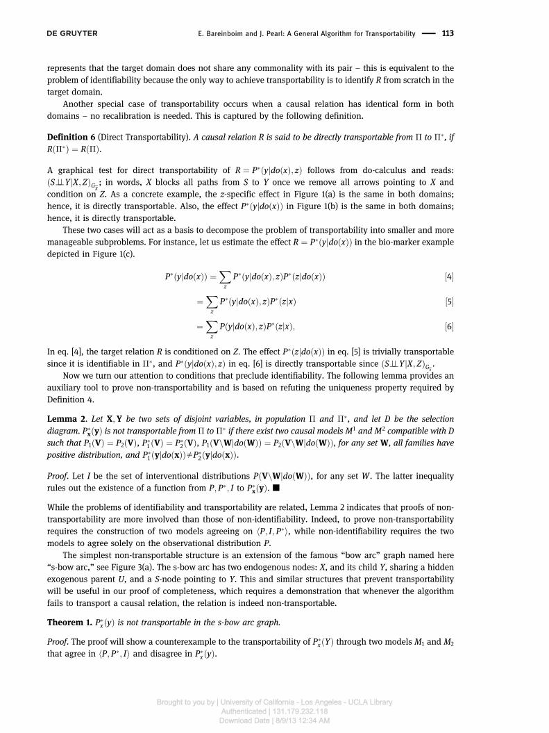
The simplest non-transportable structure is an extension of the famous “bow arc” graph named here“s-bow arc,” see Figure 3(a). The s-bow arc has two endogenous nodes: X, and its child Y, sharing a hiddenexogenous parent U, and a S-node pointing to Y. This and similar structures that prevent transportabilitywill be useful in our proof of completeness, which requires a demonstration that whenever the algorithmfails to transport a causal relation, the relation is indeed non-transportable.

Theorem 1. P�xðyÞ is not transportable in the s-bow arc graph.

Proof. The proof will show a counterexample to the transportability of P�xðYÞ through two models M1 and M2

that agree in hP;P�; Ii and disagree in P�xðyÞ.



Assume that all variables are binary. Let the model M1 be defined by the following system of structuralequations: X1 ¼ U;Y1 ¼ ððX # UÞ # SÞ;P1ðUÞ ¼ 1=2, and M2 by the following one: X2 ¼ U;Y2 ¼ S _ðX # UÞ; P2ðUÞ ¼ 1=2, where # represents the exclusive or function.

Lemma 3. The two models agree in the distributions hP;P�; Ii.

Proof. We show that the following equations must hold for M1 and M2:

P1ðXjSÞ ¼ P2ðXjSÞ; S ¼ f0; 1gP1ðY jX; SÞ ¼ P2ðY jX; SÞ; S ¼ f0; 1gP1ðY jdoðXÞ; S ¼ 0Þ ¼ P2ðY jdoðXÞ; S ¼ 0Þ

8<:

for all values of X;Y . The equality between PiðXjSÞ is obvious since ðS\\XÞ and X has the same structuralform in both models. Second, let us construct the truth table for Y:

X S U Y1 Y1

0 0 0 0 00 0 1 1 10 1 0 1 10 1 1 0 11 0 0 1 11 0 1 0 01 1 0 0 11 1 1 1 1

To show that the equality between PiðY ¼ 1jX; S ¼ 0Þ;X ¼ f0; 1g holds, we rewrite it as follows:

PiðY ¼ 1jX; S ¼ 0Þ ¼ PiðY ¼ 1jX; S ¼ 0;U ¼ 1ÞPiðXjU ¼ 1ÞPiðU ¼ 1ÞPiðXÞ

þ PiðY ¼ 1jX; S ¼ 0;U ¼ 0ÞPiðXjU ¼ 0ÞPiðU ¼ 0ÞPiðXÞ

½7�

In eq. [7], the expressions for X ¼ f0; 1g are functions of the tuples fðX ¼ 1; S ¼ 0;U ¼ 1Þ;ðX ¼ 0; S ¼ 0;U ¼ 0Þg, which evaluate to the same value in both models. Similarly, the expressionsPiðY ¼ 1jX; S ¼ 1Þ for X ¼ f0; 1g are functions of the tuples fðX ¼ 1; S ¼ 1;U ¼ 1Þ; ðX ¼ 0; S ¼ 1;U ¼ 0Þg,which also evaluate to the same value in both models.

We further assert the equality between the interventional distributions in �, which can be written usingthe do-calculus as

PiðY ¼ 1jdoðXÞ; S ¼ 0Þ ¼XU

PiðY jdoðXÞ; S ¼ 0;UÞPiðUjdoðXÞ; S ¼ 0Þ

¼ PiðY ¼ 1jX; S ¼ 0;U ¼ 1ÞPiðU ¼ 1Þþ PiðY ¼ 1jX; S ¼ 0;U ¼ 0ÞPiðU ¼ 0Þ; X ¼ f0; 1g

½8�

Evaluating this expression points to the tuples fðX ¼ 1; S ¼ 0;U ¼ 1Þ; ðX ¼ 1; S ¼ 0;U ¼ 0Þg andfðX ¼ 0; S ¼ 0;U ¼ 1Þ; ðX ¼ 0; S ¼ 0;U ¼ 0Þg, which map to the same value in both models. ■

Lemma 4. There exist values of X;Y such that P1ðY jdoðXÞ; S ¼ 1Þ�P2ðY jdoðXÞ; S ¼ 1Þ.

Proof. Fix X ¼ 1;Y ¼ 1, and let us rewrite the desired quantity in �� as



PiðY ¼ 1jdoðX ¼ 1Þ; S ¼ 1Þ ¼XU

PiðY jdoðX ¼ 1Þ; S ¼ 1;UÞPiðUjdoðX ¼ 1Þ; S ¼ 1Þ

¼ PiðY ¼ 1jX ¼ 1; S ¼ 1;U ¼ 1ÞPiðU ¼ 1Þþ PiðY ¼ 1jX ¼ 1; S ¼ 1;U ¼ 0ÞPiðU ¼ 0Þ

½9�

Since Ri is a function of the tuples fðX ¼ 1; S ¼ 1;U ¼ 1Þ; ðX ¼ 1; S ¼ 1;U ¼ 0Þg, it evaluates in M1 to f1; 1gand in M2 to f1;0g.

Hence, together with the uniformity of PðUÞ, it follows that R1 ¼ 1 and R2 ¼ 1=2, which finishes theproof. ■

By Lemma 2, Lemmas 3 and 4 prove Theorem 1. ■

4 Characterizing transportable relations

The concept of confounded components (or C-components) was introduced in [26] to represent clusters ofvariables connected through bidirected edges and was instrumental in establishing a number of conditionsfor ordinary identification (Def. 2). If G is not a C-component itself, it can be uniquely partitioned into a setCðGÞ of C-components. We now recast C-components in the context of transportability.9

Definition 7 (sC-component). Let G be a selection diagram such that a subset of its bidirected arcs forms aspanning tree over all vertices in G. Then G is a sC-component (selection confounded component).

A special subset of C-components that embraces the ancestral set of Y was noted by Shpitser and Pearl [27]to play an important role in deciding identifiability – this observation can also be applied to transport-ability, as formulated in the next definition.

Definition 8 (sC-tree). Let G be a selection diagram such that CðGÞ ¼ fGg, all observable nodes have at mostone child, there is a node Y, which is a descendent of all nodes, and there is a selection node pointing to Y.Then G is called a Y-rooted sC-tree (selection confounded tree).

The presence of this structure (and generalizations) will prove to be an obstacle to transportability of causaleffects. For instance, the s-bow arc in Figure 3(a) is a Y-rooted sC-tree where we know P�xðyÞ is nottransportable there.

X YZ(b)

S S

(a)X Y

Figure 3 (a) Smallest selection diagram in which P�ðyjdoðxÞÞ is not transportable (s-bow graph). (b) A selection diagram inwhich even though there is no S-node pointing to Y, the effect of X on Y is still not-transportable due to the presence of a sC-tree(see Corollary 2).

9 Departing from results given in [28–32], the advent of C-components complements the notion of inducing path, which wasearlier introduced in [33], and led to a breakthrough result proving completeness of the do-calculus for non-parametricidentification of causal effects by [27, 34].



In certain classes of problems, the absence of such structures will prove sufficient for transportability.One such class is explored below and consists of models in which the set X coincides with the parents of Y.

Theorem 2. Let G be a selection diagram. Then for any node Y, the causal effects P�PaðYÞðyÞ is transportable ifthere is no subgraph of G which forms a Y-rooted sC-tree.

Proof. See Appendix 2. ■

Theorem 2 provides a tractable transportability condition for the CDE – a key concept in modern mediationanalysis, which permits the decomposition of effects into their direct and indirect components [35, 36]. CDEis defined as the effect of X on Y when all other parents of Y (acting as mediators) are held constant, and it isidentifiable if and only if P�PaðYÞðyÞ is identifiable [16, p. 128].

The selection diagram in Figure 1(a) does not contain any Y-rooted sC-trees as subgraphs and thereforethe direct effect (causal effects of Y’s parents on Y) is indeed transportable. In fact, the transportability ofCDE can be determined by a more visible criterion:

Corollary 1. Let G be a selection diagram. Then for any node Y, the direct effect P�PaðYÞðyÞ is transportable ifthere is no S node pointing to Y.


Generalizing to arbitrary effects, the following result provides a necessary condition for transportabilitywhenever the whole graph is a sC-tree.

Theorem 3. Let G be a Y-rooted sC-tree. Then the effects of any set of nodes in G on Y are not transportable.


The next corollary demonstrates that sC-trees are obstacles to the transportability of P�xðyÞ even when theydo not involve Y, i.e., transportability is not a local problem – if there exists a node W that is an ancestor ofY but not necessarily “near” it, transportability is still prohibited (see Figure 3(b)). This fact anticipates thattransporting causal effects for singletons is not necessarily easier than the general problem oftransportability.

Corollary 2. Let G be a selection diagram, and X and Y a set of variables. If there exists a node W that is anancestor of some node Y 2 Y such that there exists a W-rooted sC-tree which contains any variables in X, thenP�xðyÞ is not transportable.


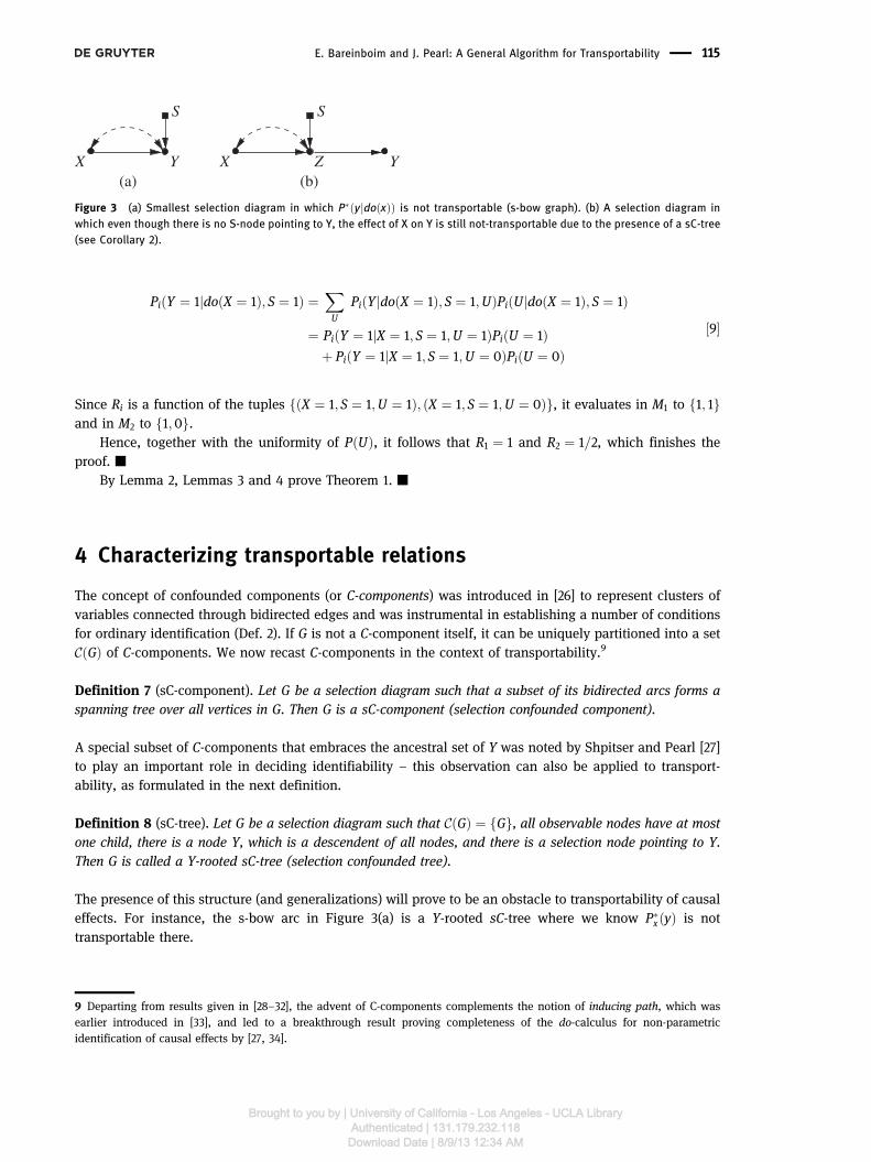
We now generalize the definition of sC-trees (and Theorem 3) in two ways: first, Y is augmented to representa set of variables; second, S-nodes can point to any variable within the sC-component, not necessarily toroot nodes. For instance, consider the graph G in Figure 4. Note that there is no Y-rooted sC-tree norW-rooted sC-tree in G (where W is an ancestor of Y), and so the previous results cannot be applied eventhough the effect of X on Y is not transportable in G – still, there exists a Y-rooted sC-forest in G, which willprevent the transportability of the causal effect.

Definition 9 (sC-forest). Let G be a selection diagram, where Y is the maximal root set. Then G is a Y-rootedsC-forest if G is a sC-component, all observable nodes have at most one child, and there is a selection nodepointing to some vertex of G (not necessarily in Y).

Building on [27], we introduce a structure that witnesses non-transportability characterized by a pair ofsC-forests. Transportability will be shown impossible whenever such structure exists as an edge subgraph ofthe given selection diagram.



Definition 10 (s-hedge). Let X;Y be set of variables in G. Let F; F0 be R-rooted sC-forests such that F˙X � 0,F0˙ X ¼ 0, F0 � F, R � AnðYÞG

X. Then F and F0 form a s-hedge for P�xðyÞ in G.

For instance, in Figure 4, the sC-forests F0 ¼ fC;Yg, and F ¼ F0¨ fX;A;Bg form a s-hedge to P�xðyÞ.10 Theidea here is similar to the hedge [27], and we can see a s-hedge as a growing sC-forest F0, which does notintersect X, to a larger sC-forest F that do intersect X.

We state below the formal connection between s-hedges and non-transportability.

Theorem 4. Assume there exist F; F0 that form a s-hedge for P�xðyÞ in � and ��. Then P�xðyÞ is nottransportable from � to ��.


To prove that the s-hedges characterize non-transportability in selection diagrams, we construct in the nextsection an algorithm which transport any causal effects that do not contain a s-hedge.

5 A complete algorithm for transportability of joint effects

The algorithm proposed to solve transportability is called sID (see Figure 5) and extends previous analysisand algorithms of identifiability given in [13, 26, 27, 32, 34]. We choose to start with the version provided byShpitser (called ID) since the hedge structure is explicitly employed, which will show to be instrumental toprove completeness. We build on two observations developed along the article:

1. Transportability: Causal relations can be partitioned into trivially and directly transportable.2. Non-transportability: The existence of a s-hedge as an edge subgraph of the inputted selection diagram

can be used to prove non-transportability.

The algorithm sID first applies the typical c-component decomposition on top of the inputted selectiondiagram D (which, by definition, is also a causal diagram of ��), partitioning the original problem intosmaller blocks (call these blocks sc-factors) until either the entire expression is transportable or it runs intothe problematic s-hedge structure.

More specifically, for each sc-factor Q, sID tries to directly transport Q. If it fails, sID tries to triviallytransport Q, which is equivalent to solving an ordinary identification problem. sID alternates between thesetwo types of transportability, and whenever it exhausts the possibility of applying these operations, it exitswith failure with a counterexample for transportability – that is, the graph local to the faulty call witnessesthe non-transportability of the causal query since it contains a s-hedge as edge subgraph.

Before showing the more formal properties of sID, we demonstrate how sID works through thetransportability of Q ¼ P�ðyjdoðxÞÞ in the graph in Figure 2.

YX A B C

Figure 4 Example of a selection diagram in which P�ðyjdoðxÞÞ is not transportable, there is no sC-tree but there is a sC-tree.

10 Note that, by definition, at least one S-node has to appear in both F 0; F.



Since D ¼ AnðYÞ and CðDnfXgÞ ¼ ðC0;C1;C2Þ, where C0 ¼ DðfZgÞ, C1 ¼ DðfWgÞ, and C2 ¼ DðfV ;YgÞ, weinvoke line 4 and try to transport respectively Qo ¼ P�x;w;v;yðzÞ, Q1 ¼ P�x;z;v;yðwÞ, and Q2 ¼ P�x;z;wðv; yÞ. Thus theoriginal problem reduces to transporting

Pz;w;v P

�x;w;v;yðzÞP�x;z;v;yðwÞP�x;z;wðv; yÞ.

Evaluating the first expression, sID triggers line 2, noting that nodes that are not ancestors of Z can beignored. This implies that P�x;w;v;yðzÞ ¼ P�ðzÞ with induced subgraph G0 ¼ fX ! Z;X Uxz ! Zg, where Uxz

stands for the hidden variable between X and Z. sID goes to line 5, in which in the local callCðDnfXgÞ ¼ fGZg. In the sequel, sID goes to line 9 since G0 contains only one sC-component. Note thatin the ordinary identifiability problem the procedure would fail at this point, but sID proceeds to line 10testing whether ðS\\fZgjfXgÞD

X. The test comes true, which makes sID directly transport Q0 with data from

the experimental population �, i.e., P�xðzÞ ¼ PxðzÞ.Evaluating the second expression, sID again triggers line 2, which implies that P�x;z;v;yðwÞ ¼ P�x;zðwÞ with

induced subgraph G1 ¼ fX ! Z; Z ! W ;X Uxz ! Zg. sID goes to line 5, in which in the local callCðDnfX; ZgÞ ¼ fGWg. Thus it proceeds to line 6 testing whether there are more than one sC-components.The test comes true (since GW 2 CðG1Þ), which makes sID to trivially transport Q1 with observational datafrom ��, i.e., P�x;zðwÞ ¼ P�ðwjx; zÞ.

Evaluating the third expression, sID goes to line 5 in which CðDnfX; Z;WgÞ ¼ fG2g, whereG2 ¼ fV ! Y ; S! V ;V Uvy ! Yg. It proceeds to line 6 testing whether there is more than one compo-nent, which is true in this case. It reaches line 8, in which C0 ¼ G0 ¨ G2 ¨fX Uxy ! Yg. Thus it tries totransport Q20 ¼ P�x;zðv; yÞ over the induced graph C0, which stands for ordinary identification, and yields(after trivial simplifications)

Pv P�ðvjwÞP�ðyjvÞ. The return of these calls composed coincide with the

expression provided in the first section.We prove next soundness and completeness of sID.

Theorem 5 (soundness). Whenever sID returns an expression for P�xðyÞ, it is correct.


Theorem 6. Assume sID fails to transport P�xðyÞ (executes line 11). Then there exists X0 � X, Y0 � Y, such thatthe graph pair D;C0 returned by the fail condition of sID contain as edge subgraphs sC-forests F, F0 that form as-hedge for P�x0 ðy0Þ.


Corollary 3 (completeness). sID is complete.


Figure 5 Modified version of identification algorithm capable of recognizing transportable relations.



Corollary 4. P�xðyÞ is transportable from � to �� in G if and only if there is not s-hedge for P�x0 ðy0Þ in G for anyX0 � X and Y0 � Y.


Theorem 7. The rules of do-calculus, together with standard probability manipulations are complete forestablishing transportability of all effects of the form P�xðyÞ.


6 Other perspectives on generalizability

Many problems in statistics and causal inference can be framed as problems of generalizability, thoughinherently different from that of transportability.

Consider, for example, classical statistical inference, it can be viewed as a generalization from proper-ties of a random sample �S of a population � to properties of the population � itself. Two centuries ofstatistical analysis have rendered this task well understood and fairly complete.

Next consider the problem of causal inference, that is, to estimate causal-effects from observationalstudies (given a set of causal assumptions). This class of problems can be viewed as a generalization from apopulation under observational regime to a population under experimental regime. Since the imposition ofexperimental regime (e.g., forcing individuals to receive treatment) induces a behavioral change in thepopulation, the problem can be viewed as generalization between two diverse populations. Fortunately,the disparities between the two populations are local (assumes atomic interventions), involving only thetreatment assignment mechanism and, so, with the help of model assumptions, a complete solution to theproblem can be obtained (using do-calculus). We can decide algorithmically whether the assumptions athand are sufficient for estimating a given causal effect and, if the answer is affirmative, we can derive itsestimand.

An important variant in causal inference is the task of estimating causal effects from surrogateexperiments, namely, experiments in which a surrogate set of variables Z are manipulated, rather thanthe one (X) whose effect we seek to estimate.11 This variant too can be viewed as an exercise in general-ization, this time from a population under regime doðZ ¼ zÞ to that same population under regimedoðX ¼ xÞ. A complete solution to this problem is reported in [37].

Another challenge of generalizability flavor arises, in both observational and experimental studies,when samples �S are not randomly drawn from the population of interest �, but are selected preferentially,depending on the values taken by a set VS of variables. This problem, known as “selection bias” (or“sampling selection bias”), has received due attention in epidemiology, statistics, and economics [38–41]and can be viewed as a generalization from the sampled population to the population at large, when little isknown about their relationships save for qualitative assumptions about the selection mechanism. Graphicalmodels were used to improve the understanding of the problem [42–45] and gave rise to several conditionsfor recovering from selection bias when the probability of selection is available.

Likewise, Refs. 21, 46, 47 tackle variants of the sample selection problem assuming that certainrelationships are invariant between the two groups (i.e., sample and population). The former assumedknowledge of the probability of selection in each of the principal stratum, while the latter exploited(using propensity score analysis) the availability of the probability of selection in each combination ofcovariates.

11 A surrogate variable is different from instrumental variable in that the former should lead to the identification of causal effecteven in nonparametric models; IV methods are limited to “local” causal effects (so-called LATE [48]).



More recently, Didelez et al. [49] studied conditions for recovering from selection bias when noquantitative knowledge is available about selection probabilities. Bareinboim and Pearl [50] extendedthese conditions and provided a complete characterization, together with an algorithm, for deciding whena bias-free estimate of the odds ratio (OR) can be recovered from selection-biased data. They also developedmethods using instrumental variables that recover other effect measures when information about the targetpopulation is available for some variables (see also Ref. 51).

The problem of transportability is fundamentally different from the other problems of generalizabilitydiscussed above. Transportability deals with two distinct populations that are different both in theirinherent characteristics (encoded by the S variables) and the regimes under which they are studied (i.e.,experimental vs. observational).

Hernán and VanderWeele [52] addressed a problem related to transportability in the context of“compound treatments,” namely, treatments that can be implemented in multiple versions (e.g., “exerciseat least 15 minutes a day”). Transportability arises when we wish to predict the response of a populationthat implements one version of the treatment from a study on another population, in which another versionis implemented. Petersen [53] showed that this problem is a variant of the general problem treated in Ref. 1,to which this article provides an algorithmic solution.

Finally, it is important to mention two recent extensions of the results reported in this article.Bareinboim and Pearl [2] have addressed the problem of transportability in cases where only a limited setof experiments can be conducted at the source environment. Subsequently, the results were generalized tothe problem of “meta-transportability,” that is, pooling experimental results from multiple and disparatesources to synthesize a consistent estimate of a causal relation at yet another environment, potentiallydifferent from each of the formers [3].

7 Conclusions

Informal discussions concerning the difficulties of generalizing experimental results across populationshave been going on for almost half a century [4, 5, 54–56] and appear to accompany every textbook inexperimental design. By and large, these discussions have led to the obvious conclusions that researchersshould be extremely cautious about unwarranted generalization, that many threats may await the unwary,and that extrapolation across studies requires “some understanding of the reasons for the differences”[54, p. 11].

The formalization offered in this article embeds this discussion in a precise mathematical language andprovides researchers with theoretical guarantees that, if certain conditions can be ascertained, general-ization across populations can be accomplished, protected from the threats and dangers that the informalliterature has accumulated.

Given judgmental assessments of how target populations may differ from those under study, the articleoffers a formal representational language for making these assessments precise (Definition 3) and, subse-quently, deciding whether, and how, causal relations in the target population can be inferred from thoseobtained in experimental studies. Corollary 4 in this article provides a complete (necessary and sufficient)graphical condition for deciding this question and, whenever satisfied, we further provide an algorithm forcomputing the correct transport formula (Figure 5). The transport formula specifies the proper way ofmodifying the experimental results so as to account for differences in the populations. These transportformulae enable the investigator to select the essential measurements in both the experimental andobservational studies and combine them into a bias-free estimand of the target quantity.

While the results of this article concern the transfer of causal information from experimental toobservational studies, the method can also benefit in transporting statistical findings from one observa-tional study to another [57]. The rationale for such transfer is twofold. First, information from the first studymay enable researchers to avoid repeated measurement of certain variables in the target population.



Second, by pooling data from both populations, we increase the precision in which their commonalities areestimated and, indirectly, also increase the precision by which the target relationship is transported.Substantial reduction in sampling variability can be thus achieved through this decomposition [58].

Of course, our analysis is based on the assumption that the analyst is in possession of sufficientbackground knowledge to determine, at least qualitatively, where two populations may differ from oneanother. In practice, such knowledge may only be partially available. Still, as in every mathematicalexercise, the benefit of the analysis lies primarily in understanding what must be assumed about realityfor generalization to be valid, what knowledge is needed for a given task to succeed, and how sensitiveconclusions are to knowledge that we do not possess.

Acknowledgment: A preliminary version of this article was presented at the 26th AAAI Conference, Toronto,CA, July, 2012 [59]. We appreciate the insightful comments provided by two anonymous referees. This articlebenefited from discussions with Onyebuchi Arah, Stuart Baker, Susan Ellenberg, Eleazar Eskin, ConstantineFrangakis, Sander Greenland, David Heckerman, James Heckman, Michael Hoefler, Marshall Joffe, RosaMatzkin, Geert Molengergh, William Shadish, Ian Shrier, Dylan Small, Corwin Zigler, and Song-Chun Zhu.

This research was supported in parts by grants from NSF #IIS-1249822, and ONR #N00014–13–1-0153and #N00014–10–1-0933.

Appendix 1: causal assumptions in nonparametric models

The tools presented in this article were developed in the framework of nonparametric SCM, which subsumesand unifies many approaches to causal inference.12

ASCMM conveys a set of assumptionsabout how theworldoperates. This contrasts the statistical tradition inwhich a model is defined as a set of distributions (see footnote 15). Causal models is better viewed as a set ofassumptions aboutNature,with the understanding that each assumption (i.e., that the set of arguments of fi doesnot include variable Vj) constrains the set of distributions (like PðvÞ) that the model can generate.

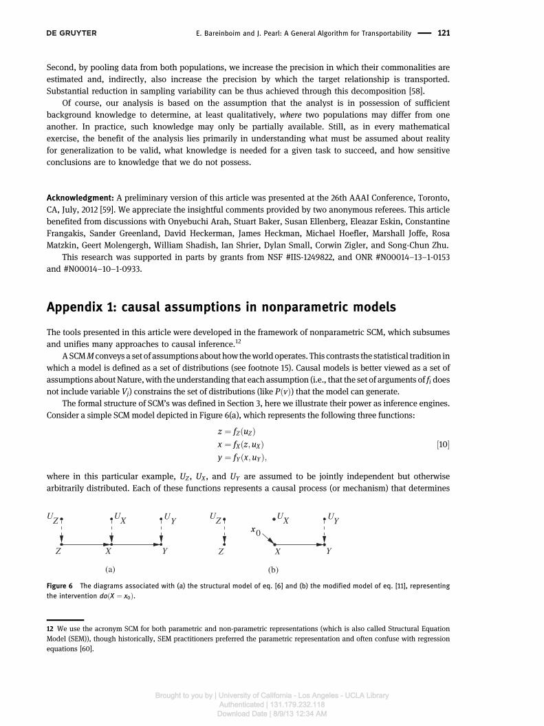
The formal structure of SCM’s was defined in Section 3, here we illustrate their power as inference engines.Consider a simple SCM model depicted in Figure 6(a), which represents the following three functions:

z ¼ fZðuZÞx ¼ fXðz; uXÞy ¼ fYðx; uYÞ;

½10�

where in this particular example, UZ, UX, and UY are assumed to be jointly independent but otherwisearbitrarily distributed. Each of these functions represents a causal process (or mechanism) that determines

Z X YZ X YU U U

Z X

0x

(b)

Y

U U U

(a)

X YZ

Figure 6 The diagrams associated with (a) the structural model of eq. [6] and (b) the modified model of eq. [11], representingthe intervention doðX ¼ x0Þ.

12 We use the acronym SCM for both parametric and non-parametric representations (which is also called Structural EquationModel (SEM)), though historically, SEM practitioners preferred the parametric representation and often confuse with regressionequations [60].



the value of the left variable (output) from the values on the right variables (inputs) and is assumed to beinvariant unless explicitly intervened on. The absence of a variable from the right-hand side of an equationencodes the assumption that nature ignores that variable in the process of determining the value of theoutput variable. For example, the absence of variable Z from the arguments of fY conveys the empiricalclaim that variations in Z will leave Y unchanged, as long as variables UY and X remain constant.

Representing Interventions, counterfactuals, and causal effects

This feature of invariance permits us to derive powerful claims about causal effects and counterfactuals,even in nonparametric models, where all functions and distributions remain unknown. This is done througha mathematical operator called doðxÞ, which simulates physical interventions by deleting certain functionsfrom the model, replacing them with a constant X ¼ x, while keeping the rest of the model unchanged[61–63]. For example, to emulate an intervention doðx0Þ that holds X constant (at X ¼ x0) in model M ofFigure 6(a), we replace the equation for x in eq. [10] with x ¼ x0, and obtain a new model, Mx0 ,

z ¼ fZðuZÞx ¼ x0y ¼ fYðx; uYÞ;

½11�

the graphical description of which is shown in Figure 6(b).The joint distribution associated with the modified model, denoted Pðz; yjdoðx0ÞÞ describes the post-

intervention distribution of variables Y and Z (also called “controlled” or “experimental” distribution), to bedistinguished from the preintervention distribution, Pðx; y; zÞ, associated with the original model of eq. [10].For example, if X represents a treatment variable, Y a response variable, and Z some covariate that affectsthe amount of treatment received, then the distribution Pðz; yjdoðx0ÞÞ gives the proportion of individualsthat would attain response level Y ¼ y and covariate level Z ¼ z under the hypothetical situation in whichtreatment X ¼ x0 is administered uniformly to the population.13

In general, we can formally define the postintervention distribution by the equation

PMðyjdoðxÞÞ ¼ PMxðyÞ ½12�In words, in the framework of model M, the postintervention distribution of outcome Y is defined as theprobability that model Mx assigns to each outcome level Y ¼ y. From this distribution, which is readilycomputed from any fully specified model M, we are able to assess treatment efficacy by comparing aspectsof this distribution at different levels of x0.

14

Identification, d-separation and causal calculus

A central question in causal analysis is the question of identification in partially specified models: Givenassumptions set A (as embodied in the model), can the controlled (postintervention) distribution,PðyjdoðxÞÞ, be estimated from data governed by the preintervention distribution Pðz; x; yÞ?

In linear parametric settings, the question of identification reduces to asking whether some modelparameter, β, has a unique solution in terms of the parameters of P (say the population covariance matrix).

13 Equivalently, Pðz; yjdoðx0ÞÞ can be interpreted as the joint probability of ðZ ¼ x;Y ¼ yÞ under a randomized experimentamong units receiving treatment level X ¼ x0. Readers versed in potential-outcome notations may interpret PðyjdoðxÞ; zÞ as theprobability PðYx ¼ yjZx ¼ zÞ, where Yx is the potential outcome under treatment X ¼ x.14 Counterfactuals are defined similarly through the equation YxðuÞ ¼ YMx ðuÞ (see [16, Ch. 7]), but will not be needed for thediscussions in this article.



In the nonparametric formulation, the notion of “has a unique solution” does not directly apply sincequantities such as QðMÞ ¼ PðyjdoðxÞÞ have no parametric signature and are defined procedurally bysimulating an intervention in a causal model M, as in eq. [11]. The following definition captures therequirement that Q be estimable from the data:

Definition 11 (Identifiability).15 A causal query QðMÞ is identifiable, given a set of assumptions A, if for anytwo models (fully specified) M1 and M2 that satisfy A, we have

PðM1Þ ¼ PðM2Þ ) QðM1Þ ¼ QðM2Þ ½13�

In words, the functional details of M1 and M2 do not matter; what matters is that the assumptions in A (e.g.,those encoded in the diagram) would constrain the variability of those details in such a way that equality ofP’s would entail equality of Q’s. When this happens, Q depends on P only, and should therefore beexpressible in terms of the parameters of P.

When a query Q is given in the form of a do-expression, for example Q ¼ PðyjdoðxÞ; zÞ, its identifiabilitycan be decided systematically using an algebraic procedure known as the do-calculus [13]. It consists ofthree inference rules that permit us to map interventional and observational distributions whenever certainconditions hold in the causal diagram G.

The conditions that permit the application these inference rules can be read off the diagrams using agraphical criterion known as d-separation [65].

Definition 12 (d-separation). A set S of nodes is said to block a path p if either

1. p contains at least one arrow-emitting node that is in S, or2. p contains at least one collision node that is outside S and has no descendant in S.

If S blocks all paths from set X to set Y, it is said to “d-separate X and Y ; ” and then, it can be shown thatvariables X and Y are independent given S, written X\\Y jS.16

D-separation reflects conditional independencies that hold in any distribution PðvÞ that is compatible withthe causal assumptions A embedded in the diagram. To illustrate, the path UZ ! Z ! X ! Y in Figure 6(a)is blocked by S ¼ fZg and by S ¼ fXg, since each emits an arrow along that path. Consequently we caninfer that the conditional independencies UZ \\Y jZ and UZ \\Y jX will be satisfied in any probabilityfunction that this model can generate, regardless of how we parametrize the arrows. Likewise, the pathUZ ! Z ! X UX is blocked by the null set f�g, but it is not blocked by S ¼ fYg since Y is a descendantof the collision node X. Consequently, the marginal independence UZ \\UX will hold in the distribution, butUZ \\UX jY may or may not hold.17

The rules of do-calculus

Let X, Y, Z, and W be arbitrary disjoint sets of nodes in a causal DAG G. We denote by GX the graph obtainedby deleting from G all arrows pointing to nodes in X. Likewise, we denote by GX the graph obtained by

15 This definition appears to be similar to, but differ fundamentally from the standard statistical definition [64, p. 22] whichdeals with the unidentifiability of the parameter set θ from a distribution Pθ. In our case, the query Q ¼ PðY jdoðxÞÞ is not aparameter of P (see [22, p. 77]).16 See Hayduk et al. [66], Glymour and Greenland [67], and Pearl [16, p. 335] for a gentle introduction to d-separation.17 This special handling of collision nodes (or colliders, e.g., Z ! X Ux) reflects a general phenomenon known as Berkson’sparadox [68], whereby observations on a common consequence of two independent causes render those causes dependent. Forexample, the outcomes of two independent coins are rendered dependent by the testimony that at least one of them is a tail.



deleting from G all arrows emerging from nodes in X. To represent the deletion of both incoming andoutgoing arrows, we use the notation GXZ .

The following three rules are valid for every interventional distribution compatible with G.

Rule 1 (Insertion/deletion of observations):

PðyjdoðxÞ; z;wÞ ¼ PðyjdoðxÞ;wÞ if ðY \\ ZjX;WÞGX

½14�

Rule 2 (Action/observation exchange):

PðyjdoðxÞ; doðzÞ;wÞ ¼ PðyjdoðxÞ; z;wÞ if ðY \\ ZjX;WÞGXZ

½15�

Rule 3 (Insertion/deletion of actions):

PðyjdoðxÞ; doðzÞ;wÞ ¼ PðyjdoðxÞ;wÞ if ðY \\ ZjX;WÞGXZðWÞ

; ½16�

where ZðWÞ is the set of Z-nodes that are not ancestors of any W-node in GX.To establish identifiability of a query Q, one needs to repeatedly apply the rules of do-calculus to Q,

until the final expression no longer contains a do-operator18; this renders it estimable from non-experi-mental data. The do-calculus was proven to be complete to the identifiability of causal effects in the formQ ¼ PðyjdoðxÞ; zÞ [69, 70], which means that if Q cannot be expressed in terms of the probability ofobservables P by repeated application of these three rules, such an expression does not exist.

We shall see that, to establish transportability, the goal will be different; instead of eliminating do-operators, we will need to separate them from a set of variables S that represent disparities betweenpopulations.

Appendix 2

Theorem 2. Let G be a selection diagram. Then for any node Y, the direct effect P�PaðYÞðyÞ is transportable ifthere is no subgraph of G which forms a Y-rooted sC-tree.

Proof. We known from Tian [71, Theorem 22] that whenever there exists no subgraph GT of G satisfying all ofthe following: (i) Y 2 T; (ii) GT has only one c-component, T itself; (iii) All variables in T are ancestors of Yin GT , the direct effect on Y is identifiable, as sC-trees are structures of this type. Further Shpitser and Pearl[27, Theorem 2] showed that the same holds for C-trees, which also implies the inexistence of a sC-trees.Since such structure does not show up in G, the target quantity is identifiable, and hence transportable.

It remains to show that the same holds whenever there exists a subgraph that is a C-tree and in whichno S node points to Y, i.e., there is no Y-rooted sC-tree at all. It is true that ðS\\Y jPaðYÞÞG

PaðYÞ, given that all

directed paths from S to Y are closed. This follows from the following facts: (1) all paths from S passingthrough Y’s ancestors were cut in GPaðYÞ; (2) all bidirected paths were also closed given that the conditioningset contains only root nodes, and a connection from S must pass through at least one collider; (3)transportability does not depend on descendants of Y (by argument similar to Tian [71, Lemma 9]). Thus,it follows that we can write P�PaðYÞðYÞ ¼ PPaðYÞðY jSÞ ¼ PPaðYÞðYÞ, concluding the proof. ■

Corollary 1. Let G be a selection diagram. Then for any node Y, the direct effect P�PaðYÞðyÞ is transportable ifthere is no S node pointing to Y.

Proof. Follows directly from Theorem 2. ■

18 Such derivations are illustrated in graphical details in Ref. [16, p. 87].



Lemma 5. The exclusive OR (XOR) function is commutative and associative.

Proof. Follows directly from the definition of the XOR function. ■

Remark 1. The construction given below is a strict generalization of Theorem 1, and it is useful because itwill provide a simplified construction of the one provided in Theorem 1, and also set the tone for proofs ofgeneric graph structures which will in the sequel show to be instrumental in proving non-transportability inarbitrary structures.

Theorem 3. Let G be a Y-rooted sC-tree. Then the effects of any set of nodes in G on Y are nottransportable.

Proof. The proof will proceed by constructing a family of counterexamples. For any such G and any set X,we will construct two causal models M1 and M2 that will agree on hP;P�; Ii, but disagree on the interven-tional distribution P�xðyÞ.

Let the two models M1, M2 agree on the following features. All variables in U ¨ V are binary. All exogenousvariables are distributed uniformly. All endogenous variables except Y are set to the bit parity (sum mod 2)of the values of their parents. The two models differ in respect to Y’s definition. Consider the function for Y,fY : U;PaðYÞ ! Y to be defined as follows:

M1 : Y ¼ ððpaðYÞ # uÞ # sÞM2 : Y ¼ ððpaðYÞ # uÞ _ sÞ

�


Proof. Since the two models agree on PðUÞ and all functions except fY , it suffices to show that fY maintainsthe same input/output behavior in both models for each domains.

Subclaim 1: Let us show that both models agree in the observational and interventional distributionsrelative to domain �, i.e., the pair hP; Ii. The index variable S is set to 0 in �, and fY evaluates toðpaðYÞ # uÞ in both models, which proves the subclaim.

Subclaim 2: Let us show that both models agree in the observational distribution relative to ��, i.e., P�. Theindex variable S is set 1 in��, and fY evaluates to ððpaðYÞ # uÞ # 1Þ inM1, and 1 inM2. Since the evaluation inM1 can be rewritten as :ððpaðYÞ # uÞ, it remains to show that ðpaðYÞ # uÞ always evaluates to 0.

This fact is certainly true, consider the following observations: a) each variable in U has exactly twoendogenous children; b) the given tree has Y as the root; c) all functions are XOR – these imply that Y iscomputing the bit parity of the sum of all U nodes, which turns out to be even, and so evaluates to 0 andproves the subclaim. ■

Lemma 7. For any set X, P1ðY jdoðXÞ; S ¼ 1Þ�P2ðY jdoðXÞ; S ¼ 1Þ.

Proof. Given the functional description and the discussion in the previous Lemma, the function fY evaluatesalways to 1 in M2.

Now let us consider M1. Note that performing the intervention and cutting the edges going toward Xcreates an asymmetry on the sum of the bidirected edges departing from U, and consequently in the sumperformed by Y. It will be the case that some U0 will appear only once in the expression of Y. Therefore,depending on the assignment X ¼ x, we will need to evaluate the sum (mod 2) over U0 in Y or its negation,which given the uniformity of the distribution of U will yield P1ðY jdoðXÞ; S ¼ 1Þ ¼ 1=2 in both cases. ■

By Lemma 2, Lemmas 6 and 7 together prove Theorem 3. ■



Corollary 2. Let G be a selection diagram, let X and Y be set of variables. If there exists a node W which is anancestor of some node Y 2 Y and such that there exists a W-rooted sC-tree which contains any variables in X,then P�xðyÞ is not transportable.

Proof. Fix a W-rooted sC-tree T, and a path p from W to Y. Consider the graph p ¨ T. Note that in this graphP�xðYÞ ¼

Pw P�xðwÞP�ðY jwÞ. From the last Theorem P�xðwÞ is not transportable, it is now easy to construct

P�ðY jWÞ in such a way that the mapping from PxðWÞ to PxðYÞ is one to one, while making sure alldistributions are positive.

Remark 2. The previous results comprised cases in which there exist sC-trees involved in the non-transportability of Y – i.e., Y or some of its ancestors were roots of a given sC-tree. In the problem ofidentifiability, the counterpart of sC-trees (i.e., C-trees) suffices to characterize non-identifiability forsingleton Y. But transportability is more subtle and this is not the case here – it not only depends on Xand Y “locations” in the graph, but also the relative position of the S-nodes. Consider Figures 4 and 7(a)(called sp-graph). In these graphs there is no sC-tree but the effect of X on Y is still non-transportable.

Themain technical subtlety here is that in sC-trees, a S-node combines its effect with a X-node intersecting in theroot node (considering only the bidirected edges), which is not the case for non-transportability in general. Notethat in the graphs in Figure 4, and the sp-graph, the nodes S andX intersect first throughordinary edges andmeetthroughbidirectededges onlyon theYnode.This implies a certain “asynchrony”because, in the structural sense,the existence of a S-node implies a difference in the structural equations between domains, but only thisdifference does not imply non-transportability (for instance, P�xðzÞ is transportable in the sp-graph even thoughthe equations of Z being different in both models).

The key idea to produce a proof for non-transportability in these cases is to keep the effect of S-nodes afterintersecting with X “dormant” until they reach the target Y and then manifest. We implement this idea in thenext two proofs, which can be seen as base cases, and should pavement the way for the most generalproblem.

Theorem 8. P�xðyÞ is not transportable in the sp-graph (Figure 7(a)).

Proof. We will construct two causal models M1 and M2 compatible with the sp-graph that will agree onhP;P�; Ii, but disagree on the interventional distribution P�xðyÞ.

Let us assume that all variables in U ¨ V are binary, and let U1 be the common cause of X and Y, U2 be thecommon cause of Z and Y, and U3 be the random disturbance exclusive to Z. Let M1 and M2 be defined asfollows:

YX

(a)

X Y

(b)

Z

Z

S

S

Figure 7 Selection diagrams in which P�ðyjdoðxÞÞ is not transportable, there is no sC-tree but there is a sC-forest. Thesediagrams will be used as basis for the general case; the first diagram is named sp-graph and the second one sb-graph.



M1 ¼X ¼ U1

Z ¼ ðððX # U2 # 1Þ # U3Þ _ SÞ # ðS ^ ðX # U2ÞÞY ¼ Z # U1 # U2

8><>:

and:

M2 ¼X ¼ U1

Z ¼ ðððU2 # 1Þ # U3Þ _ SÞ # ðS ^ U2ÞY ¼ Z # U2

8<:

Both models agree in respect to PðUÞ, which is defined as follows: PðU1Þ ¼ PðU2Þ ¼ PðU3Þ ¼ 1=2.


Proof. Subclaim 1: Let us show that both models agree in the observational and interventional distributionsrelative to domain �, i.e., the pair hP; Ii. In both models X has the same expression, which entails the same(uniform) probabilistic behavior in both cases. The index variable S is set to 0 in �, and Z evaluates toðX # U2 # 1 # U3Þ in M1 and ðU2 # 1 # U3Þ in M2. Clearly, for any value of X ¼ x, since U is the sameand uniformly distributed in both models, we obtain the same (uniform) input/output probabilistic behaviorin M1 and M2 (note that U2;U3 can freely vary independently of X). In similar way, Y evaluates to ð1þ U3Þ inboth models, which entails the same (uniform) input/output probabilistic behavior in both models. Inregard to doðX ¼ xÞ, it is clear that Z did not depend (probabilistically) on the specific value of X, and so theequality between both models follows. For the case when we have doðZ ¼ zÞ, Y evaluates to ðZ # U1 # U2Þin M1 and ðZ # U2Þ in M2, and given the uniformity of U, they preserve the same (uniform) input/outputprobabilistic behavior. (For a more elaborated argument, see Theorem 4 below.)

Subclaim 2: Let us show that both models agree in the observational distribution P� relative to ��. Theindex variable S is set 1 in ��, fZ evaluates to ðX # U2 # 1Þ in M1, and ðU2 # 1Þ in M2. Again, for any valueof X, together with the uniformity of U, we obtain the same (uniform) input/output probabilistic behavior inboth models (note again that U2 can freely vary independently of variations of X, and so Z). Further, fYevaluates to 1 in both models, which yields the same (uniform) input/output behavior in both models. (Toguarantee positivity, we can apply the trick of making a new fY 0 ðÞ such that fY 0 ðÞ returns 0 half the time, andfY the other half (i.e., set fy0 ðÞ ¼ ½fyðÞ ^ C�, where C is a fair coin.) ■

Lemma 9. There exist values of such that X;Y P1ðY jdoðXÞ; S ¼ 1Þ�P2ðY jdoðXÞ; S ¼ 1Þ.

Proof. Fix X ¼ 1;Y ¼ 1. First notice that fZ evaluates to U2 in M1 and ðU2 # 1Þ in M2. Given that U2 isuniformly distributed, both quantities coincide (and they represent the effect of X on Z, which is transpor-table in G). Now the evaluation of fY in M1 reduces to U1, while it reduces to 1 in M2, which showdisagreement and finishes the proof of this Lemma. ■


Remark 3. There exists a different sort of asymmetry in the case of Figure 7(b) (called sb-graph), and the nodesXand S do not intersect before meeting Y – i.e., they have disjoint paths and Y lies precisely in their intersection.

Still, this case is not the same of having a sC-tree because in sb-graphs we need to keep the equality fromthe S nodes to Y until S intersects X on Y. Employing a similar construct as in the sp-graph, we keep theeffect of S dormant until it reaches Y and then emerges.

Theorem 9. P�xðyÞ is not transportable in the sb-graph (Figure 7(b)).

Proof. We construct two causal models M1 and M2 compatible with the sb-graph that will agree on hP;P�; Ii,but disagree on the interventional distribution P�xðyÞ.



Let us assume that all variables in U ¨ V are binary, and let U1 be the common cause of X and Y, U2 bethe common cause of Z and Y, and U3 be the random disturbance exclusive to X. Let M1 and M2 agree withthe following definitions:

M1;M2 ¼ X ¼ U1

Z ¼ ððU3 # U2 # 1Þ _ SÞ # ðS ^ U2ÞÞ�

and disagree in respect to Z as follows:

M1 : Y ¼ Z # U2

M2 : Y ¼ X # Z # U1 # U2

�

Both models also agree in respect to PðUÞ, which is defined as follows:

PðU1Þ ¼ PðU2Þ ¼ PðU3Þ ¼ 1=2

.Lemma 10. The two models agree in the distributions hP;P�; Ii.

Proof. Subclaim 1: Let us show that both models agree in the observational and interventional distributionsrelative to domain �, i.e., the pair hP; Ii. The index variable S is set to 0 in �, and fX; Zg are defined in thesame way in both models, and so it suffices to analyze Y, which in this case evaluates to ðU3 # 1Þ in bothmodels, preserving the same (uniform) probabilistic behavior. Given that, it is not difficult to see that bothmodels also evaluate in the same way when considering the interventions in I.

Subclaim 2: Let us show that both models agree in the observational distribution P� relative to ��. Theindex variable S is set 1 in ��, given that fX; Zg are defined in the same way in both models, together withthe uniformity of U make them evaluate in the same way in both models, and Y evaluates to 1 in bothmodels. (As in Lemma 8, the same trick to make the distribution positive could be applied here.) ■

Lemma 11. There exist values of X;Y such that P1ðY jdoðXÞ; S ¼ 1Þ � P2ðY jdoðXÞ; S ¼ 1Þ.

Proof. Fix X ¼ 1;Y ¼ 1. First notice that fZ evaluates to ðU2 # 1Þ in both models, and the evaluation of fY inM1

reduces to 1, while it reduces to U1 inM2. It follows that inM1, fY evaluates to 1 with probability 1, while inM2 itevaluates to 1 with probability PðU1 ¼ 1Þ, which disagree by construction, finishing the proof of this Lemma.■


Remark 4. There are two complementary components to forge a general scheme to prove arbitrary non-transportability. First, the construct of Theorem 4 shows how to prove non-transportability for general structuressuch as sC-trees. In the sequel, the specific proofs of non-transportability for the sp-graph (Theorem 9) and sb-graph (Theorem 10) partition the possible interactions between X, S and Y. In the former, X and S intersect beforemeetingwith Y,while in the latter they have disjoint paths and Y lies in their intersection. In the sequel, the prooffor the general case combines these analyses, which we show below.

Theorem 4. Assume there exist F; F0 that form a s-hedge for P�xðyÞ in � and ��. Then P�xðyÞ is nottransportable from � to ��.

Proof. We first consider counterexamples with the induced graph H ¼ DeðFÞG˙AnðYÞGX, and assume,

without loss of generality, that H is a forest. We construct two causal models M1 and M2 that will agreeon hP;P�; Ii, but disagree on the interventional distribution P�xðyÞ.

Let F be an R-rooted sC-forest, let V0 be the set of observable variables and U0 be the set of unobservablevariables in F. Let us assume that all variables in U0 ¨ V0 are binary. Call W the set of variables pointed byS-nodes in F0, which by the definition of sC-forest is guaranteed to be non-empty.



In model 1, let each Vi 2 V0nW compute the bit parity of all its observable and unobservable parents(i.e., f ð1Þi ¼ # ðSVj2Pai VjÞ, where the xor is applied for each element of the set and the result computed sofar), while in model 2, let Vi compute the bit parity of all its parents except that any node in F0 disregards theparents values if the parent is in F (i.e., f ð2Þi ¼#ðSVj2Pai˙F0 VjÞ if Vi is in F0, and f ð2Þi ¼ f ð1Þi , otherwise).

Define W 2 W as follows:

M1 : W ¼ ððf ð1Þw #U�wÞ _ SÞ#ðS ^ ð1#f ð1Þw ÞÞM2 : W ¼ ððf ð2Þw #U�wÞ _ SÞ#ðS ^ ð1#f ð2Þw ÞÞ

:

(

where fw is constructed in similar way as fi in M1 and M2 above, and U�w is an additional fair coin exclusivelypointing to W. Let us call Uw the collection of such coins. Furthermore, let us assume that eachUi 2 fU0nUwg is also a fair coin (i.e., PðUiÞ ¼ 1=2).

Lemma 12. The two models agree in the distribution of P� and there exists a value assignment x for X suchthat P1ðYjdoðxÞ; S ¼ 1Þ�P2ðYjdoðxÞ; S ¼ 1Þ.

Proof. For S ¼ 1, the result follows directly since the systems of equations in both models reduce to theconstruction given in Theorem 4 at [27]. ■

Lemma 13. The two models agree in the distributions hP; Ii.

Proof. Let us show that both models agree in the observational distribution P relative to domain �. Theselection variable S is set to 0 in �, and note that both systems are the same as in �� except that now eachvariable W 2W has an extra variable U�w pointing to it that should be taken into account in W’s evaluation,and in turn in the whole system.

We have a forest over the endogenous nodes and all functions compute the bit parity of the value of theirparents, and so we can view each node as computing the sum mod 2 of its exogenous ancestors in H. Wewant to show that the distribution of each family is equally likely for each possible assignment (i.e.,PðvijpaiÞ ¼ 1=2, for all vi;pai).

Let us partition the analysis in two cases. First consider the case of Vi 2 R in which there exists a S-nodein the respective sC-tree. Note that the evaluation of Vi relies only on the value of U�w 2 Uw in its respectivetree since U 2 fU0nUwg has an even number of endogenous children in F, and it is counted twice, soevaluates to zero (i.e., it does not affect Vi’s evaluation). For now, let us assume that there is only one U�wthat affects the evaluation of Vi. Given the uniformity of U�w, it suffices to show that U�w can varyindependently for any configuration of the parents of Vi.

For any configuration of U0 ¼ ðU1 ¼ u1; :::;U�w ¼ u�w; :::Þ, consider the corresponding evaluation ofPai ¼ pai, and also Vi ¼ u�w. We want to show that it is possible to flip the current value of U�w from u�wto :u�w while preserving the parents’ evaluation pai. Assume this is not so. This implies that the evaluationof Pai and Vi count the same U’s, contradiction.

To see why, consider Pai� � Pai the set of parents of Vi that are descendents of U�w. Now, for each ofthese parents flip the minimum number of variables from UnUw, and call this set U�. (Note that this isalways possible since we need at most one U for each parent, which should exist by construction ofsC-forest.) Now, make U�w ¼ :u�w, and note that Pai ¼ pai since flipping the values of U� compensates theflip of U�w. But it is also true now that Vi evaluates to :u�w since, in the same way as before, all othervariables in fUnUwg are cancelled out in Vi’s evaluation, including the ones in U�. This proves the claim.

Consider the following two facts: Subclaim 1: Let X and Y be two binary variables such thatPðX ¼ xÞ ¼ p � 1=2 and PðY ¼ yÞ ¼ q ¼ 1=2. Then the probabilistic input/output behavior ofZ ¼ XORðX;YÞ is the same of Y. The variable Z ¼ 1 whenever fðX ¼ 1;Y ¼ 0Þ; ðX ¼ 0;Y ¼ 1Þg, whichhappens with probability pqþ ð1� pÞð1� qÞ. Since q ¼ 1=2, the expression reduces top � 1=2þ ð1� pÞ � 1=2 ¼ 1=2.



Subclaim 2: Let X and Y be two binary variables such that PðX ¼ xÞ ¼ PðY ¼ yÞ ¼ p ¼ 1=2. Then theprobabilistic input/output behavior of Z ¼ XORðX;YÞ is the same of X (or Y). This follows directly fromSubclaim 1. It is clear that if there are multiple nodes from Uw in the evaluation of Vi, thesame construction is also valid given the subclaim above. It is also not difficult to generalize thisargument to consider root set that are not singleton, including roots in which there are not S-nodes asancestors.

Finally, let us consider the case of Vi 2 fFnRg. It suffices to show that the function from U0nUw to V0nRis 1–1 when we fix Uw ¼ uw. We use the same argument as Shpitser. Assume this is not so, and fix twoinstantiations of U0nUw that map to the same value of V0nR, and differ by the set U� ¼ fU1; :::;Ukg. Since thebidirected edges form a spanning tree, there exists V� with an odd number of parents in U� (and were not inR, by construction). Order them topologically and let the topmost be called X. Note that if we flip all valuesin U�, the value of X will also flip, contradiction. Given the uniformity of U0, the claim follows. We can putthis together with the previous claim, and the result follows. We can add fair coins as the input to all othervariables outside F, which will imply the claim for the whole graph G.

In regard to the equality between I, note that given that the equality of both models holds for P, andremoving edges due to interventions will just make some nodes from U0nUw to have an odd number ofchildren, it it not difficult to see based on the previous argument that this just creates more variables thatare free to vary, which will entail the same probabilistic uniform behavior in both models. Another way tosee this fact is to consider the new exogenous variables from fUnUwg that have only one children after theintervention as analogous to U�w, and so the same argument follows. ■

Finally, Lemma 2 together with Lemmas 12 and 13 prove Theorem 4. ■

Theorem 5 (soundness). Whenever sID returns an expression for P�xðyÞ, it is correct.

Proof. Noting that the selection diagram inputted to sID is also a causal diagram over ��, and trivialtransportability is equivalent to identifiability in ��, the correctness of the identifiability calls was alreadyestablished elsewhere [27, 34].

It remains to show the correctness of the test in line 10 of sID. First note that, by construction, X0 in eachlocal call is always a set of pre-treatment covariates. But now the correctness follows directly byS-admissibility of X0 together with Corollary 1 in Ref. 1. Further note that the set of Z-nodes outside thelocal component will not affect separability of the S-nodes inside it (following the topology of the hedge),and other S-nodes outside can be removed from the expression before the test. More specifically, note thatthe effect Q� in each local call that uses line 10 can be expressed in its expanded form (using a typicalC-component decomposition), and given that the independence imposed by S-admissibility holds, togetherwith the fact that both populations share the same causal graph G, allow that the functions of �� to bereplaced with the respective functions in �, which implies the result. ■

Remark 5. The next results are similar to the identification counterparts given in Refs. 26, 69.

Theorem 6. Assume sID fails to transport P�xðyÞ (executes line 11). Then there exists X0 � X, Y0 � Y, such thatthe graph pair D;C0 returned by the fail condition of sID contain as edge subgraphs sC-forests F, F0 that form as-hedge for P�x0 ðy0Þ.

Proof. Before failure sID evaluated false consecutively at lines 5, 6, and 10, so D local to this call is asC-component, and let R be its root set. We can remove some directed arrows from D while preserving R asroot, yielding a R-rooted sC-forests F. Since by construction F0 ¼ F˙C0 is closed under descendants andonly directed arrows were removed, both F; F0 are sC-forests. Also by construction, R � AnðYÞD

Xtogether

with the fact that X and Y from the recursive call are clearly subsets of the original input, finish the proof.

Corollary 3 (completeness). sID is complete.



Proof. The result follows from Theorem 6 where P�x0 ðy0Þ is not transportable in H. But now, it is easy to addthe remaining variables from G, making them independent of H (e.g., as random coins). So, the models inthe counterexample induce G, and witness the non-transportability of P�xðyÞ.

Corollary 4. P�xðyÞ is transportable from � to �� in G if and only if there is not s-hedge for P�x0 ðy0Þ in G for anyX0 � X and Y0 � Y.

Proof. Follows directly from the previous Corollary. ■

Theorem 7. The rules of do-calculus, together with standard probability manipulations are complete forestablishing transportability of all effects of the form P�xðyÞ.

Proof. It was shown elsewhere [69] that the steps of sID but line 10 correspond to sequences of standardprobability manipulations and applications of the rules of do-calculus. The line 10 is constituted by aconditional independence judgment, and standard probability operations for the replacement of the func-tions based on the invariance allowed by the S-admissibility of the local X0 in each recursive call (asdiscussed above in the proof of correctness). ■

References

1. Pearl J, Bareinboim E. Transportability of causal and statistical relations: a formal approach. In Proceedings of the Twenty-Fifth National Conference on Artificial Intelligence (AAAI 2011). Menlo Park, CA: AAAI Press, 2011:247–54.

2. Bareinboim E, Pearl J. Causal transportability with limited experiments. In Proceedings of the Twenty-Seventh AAAIConference on Artificial Intelligence (AAAI 2013), Menlo Park, CA: AAAI Press, 2013, forthcoming.

3. Bareinboim E, Pearl J. Meta-transportability of causal effects: A formal approach. In Proceedings of the SixteenthInternational Conference on Artificial Intelligence and Statistics (AISTATS 2013), 2013, forthcoming.

4. Campbell D, Stanley J. Experimental and quasi-experimental designs for research. Chicago: Wadsworth Publishing, 1963.5. Manski C. Identification for prediction and decision. Cambridge, Massachusetts: Harvard University Press, 2007.6. Glass GV. Primary, secondary, and meta-analysis of research. Educ Res 1976;5:3–8.7. Hedges LV, Olkin I. Statistical methods for meta-analysis. Orlando, Fl: Academic Press, 1985.8. Owen AB. Karl pearsons meta-analysis revisited. Ann Stat 2009;37:3867–92.9. Höfler M, Gloster A, Hoyer J. Causal effects in psychotherapy: counterfactuals counteract overgeneralization. Psychother

Res 2010, DOI: 10.1080/10503307.2010.501041.10. Shadish W, Cook T, Campbell D. Experimental and Quasi-Experimental Designs for Generalized Causal Inference. Boston:

Houghton-Mifflin, 2nd ed., 2002.11. Adelman L. Experiments, quasi-experiments, and case studies: a review of empirical methods for evaluating decision

support systems. Systems, Man and Cybernetics, IEEE Transactions on, 1991;21:93–301.12. Morgan S, Winship C. Counterfactuals and causal inference: methods and principles for social research (Analytical

Methods for Social Research). New York: Cambridge University Press, 2007.13. Pearl J. Causal diagrams for empirical research. Biometrika 1995;82:669–710.14. Greenland S, Pearl J, Robins J. Causal diagrams for epidemiologic research. Epidemiology 1999;10:37–48.15. Spirtes P, Glymour C, Scheines R. Causation, prediction, and search. Cambridge, MA: MIT Press, 2nd ed., 2001.16. Pearl J. Causality: models, reasoning, and inference. New York: Cambridge University Press, 2nd ed., 2009.17. Koller D, Friedman N. Probabilistic graphical models: principles and techniques. Cambridge, MA: MIT Press, 2009.18. Westergaard H. Scope and method of statistics. Am Stat Assoc 1916:15:229–76.19. Yule G. On some points relating to vital statistics, more especially statistics of occupational mortality. J R Stat Soc

1934;97:1–84.20. Lane P, Nelder J. Analysis of covariance and standardization as instances of prediction. Biometrics 1982;38:613–21.21. Cole S, Stuart E. Generalizing evidence from randomized clinical trials to target populations. Am J Epidemiol 2010;172:

107–15.22. Pearl J. Causality: models, reasoning, and inference. New York: Cambridge University Press, 2nd ed., 2000.23. Pearl J. Causal inference in statistics: an overview. Stat Surv 2009;3:96–146.24. Pearl J, Verma T. A theory of inferred causation. In Allen J, Fikes R, Sandewall E, editors. Principles of knowledge

representation and reasoning: Proceedings of the Second International Conference. San Mateo, CA: Morgan Kaufmann,1991:441–52.



25. Bareinboim E, Brito C, Pearl J. Local characterizations of causal bayesian networks. In Croitoru M, Corby O, Howse J,Rudolph S, Wilson N, editors. GKR-IJCAI, Lecture Notes in Artificial Intelligence (7205), Springer-Verlag, 2012:1–17.

26. Tian J, Pearl J. A general identification condition for causal effects. In Proceedings of the Eighteenth National Conference onArtificial Intelligence (AAAI 2002). Menlo Park, CA: AAAI Press/The MIT Press, 2002:567–73.

27. Shpitser I, Pearl J. Identification of joint interventional distributions in recursive semi-Markovian causal models. InProceedings of the Twenty-First National Conference on Artificial Intelligence (AAAI 2006). Menlo Park, CA: AAAI Press,2006:1219–26.

28. Spirtes P, Glymour C, Scheines R. Causation, prediction, and search. New York: Springer-Verlag, 1993.29. Galles D, Pearl J. Testing identifiability of causal effects. In Besnard P, Hanks S, editors. Proceedings of the Eleventh

Conference on Uncertainty in Artificial Intelligence (UAI 1995). San Francisco: Morgan Kaufmann, 1995:185–95.30. Pearl J, Robins J. Probabilistic evaluation of sequential plans from causal models with hidden variables. In Besnard P,

Hanks S, editors. Proceedings of the Eleventh Conference on Uncertainty in Artificial Intelligence (UAI 1995). San Francisco:Morgan Kaufmann, 1995:444–53.

31. Halpern J. Axiomatizing causal reasoning. In Cooper G, Moral S, editors. Uncertainty in artificial intelligence. SanFrancisco, CA: Morgan Kaufmann, 1998:202–10, also J Artif Intell Res 2000;12:3, 17–37.

32. Kuroki M, Miyakawa M. Identifiability criteria for causal effects of joint interventions. J R Stat Soc 1999;29:105–17.33. Verma T, Pearl J. Equivalence and synthesis of causal models. In Proceedings of the Sixth Conference on Uncertainty

in Artificial Intelligence (UAI 1990). Cambridge, MA, 1990:220–27, also in Bonissone P, Henrion M, Kanal LN, LemmerJF, editors. Uncertainty in artificial intelligence 6. Amsterdam, The Netherlands: Elsevier Science Publishers, B.V.,1990:255–68, 1991.

34. Huang Y, Valtorta M. Identifiability in causal bayesian networks: A sound and complete algorithm. In Proceedings of theTwenty-First National Conference on Artificial Intelligence (AAAI 2006). Menlo Park, CA: AAAI Press, 2006:1149–56.

35. Pearl J. Direct and indirect effects. In Proceedings of the Seventeenth Conference on Uncertainty in Artificial Intelligence(UAI 2001). San Francisco, CA: Morgan Kaufmann, 2001:411–20.

36. Pearl J. The mediation formula: A guide to the assessment of causal pathways in nonlinear models. In Berzuini C, Dawid P,Bernardinell L, editors. Causality: statistical perspectives and applications. New York: Wiley, Chapter 12, 2012.

37. Bareinboim E, Pearl, J. Causal inference by surrogate experiments: z-identifiability. In de Freitas N, Murphy K, editors.Proceedings of the Twenty-Eighth Conference on Uncertainty in Artificial Intelligence (UAI 2012), AUAI Press, 2012, 113–20.

38. Cornfield J. A method of estimating comparative rates from clinical data; applications to cancer of the lung, breast, andcervix. J Natl Cancer Inst 1951;11:1269–75.

39. Whittemore A. Collapsibility of multidimensional contingency tables. J R Stat Soc, B 1978;40:328–40.40. Geng Z, Guo J, Fung W-K. Criteria for confounders in epidemiological studies. J Royal Stat Soc Series B 2002;64:3–15.41. Heckman JJ. Sample selection bias as a specification error. Econometrica 1979;47:153–61.42. Robins JM, Hernan M, Brumback B. Marginal structural models and causal inference in epidemiology. Epidemiology

2000;11:550–60.43. Hernán M, Hernández-Díaz S, Robins J. A structural approach to selection bias. Epidemiology 2004;15:615–25.44. Lauritzen SL, Richardson TS. Discussion of mccullagh: sampling bias and logistic models. J R Stat Soc Ser B 2008;70:

140–50.45. Geneletti S, Richardson S, Best N. Adjusting for selection bias in retrospective, case-control studies. Biostatistics

2009;10:17–31.46. Weisberg H, Hayden V, Pontes V. Selection criteria and generalizability within the counterfactual framework: explaining the

paradox of antidepressant-induced suicidality? Clin Trials 2009;6:109–18.47. Stuart EA, Cole SR, Bradshaw CP, Leaf PJ. The use of propensity scores to assess the generalizability of results from

randomized trials. Journal of the Royal Statistical Society: Series A (Statistics in Society) 2011;174:369–86.48. Angrist J, Imbens G, Rubin D. Identification of causal effects using instrumental variables (with comments). J Am Stat Assoc

1996;91:444–72.49. Didelez V, Kreiner S, Keiding N. Graphical models for inference under outcome-dependent sampling. Stat Sci 2010;25:368–87.50. Bareinboim E, Pearl J. Controlling selection bias in causal inference. In Girolami M, Lawrence N, editors. Proceedings of The

Fifteenth International Conference on Artificial Intelligence and Statistics (AISTATS 2012), JMLR (22), 2012:100–08.51. Pearl J. A solution to a class of selection-bias problems. Technical Report R-405, Cognitive Systems Laboratory,

Department of Computer Science, UCLA, 2012.52. Hernán M, VanderWeele T. Compound treatments and transportability of causal inference. Epidemiology 2011;22:368–77.53. Petersen M. Compound treatments, transportability, and the structural causal model: the power and simplicity of causal

graphs. Epidemiology 2011;22:378–81.54. Cox D. The Planning of Experiments. New York: John Wiley and Sons, 1958.55. Heckman J. Randomization and social policy evaluation. In Manski C, Garfinkle I, editors. Evaluations: welfare and training

programs. Cambridge, MA: Harvard University Press, 1992:201–30.56. Hotz VJ, Imbens G, Mortimer JH. Predicting the efficacy of future training programs using past experiences at other

locations. J Econ 2005; 125:241–70.



57. Pearl J, Bareinboim E. Transportability of causal and statistical relations: A formal approach. Technical Report TechnicalReport r-372, Cognitive Systems Laboratory, Department of Computer Science, UCLA, 2011.

58. Pearl J. Some thoughts concerning transfer learning with applications to meta-analysis and data sharing estimation.Technical Report R-387, Cognitive Systems Laboratory, Department of Computer Science, UCLA, 2012.

59. Bareinboim E, Pearl J. Transportability of causal effects: completeness results. In Hoffmann J, Selman B, editors.Proceedings of The Twenty-Sixth Conference on Artificial Intelligence (AAAI 2012), 2012:698–704.

60. Bollen KA, Pearl J. Eight myths about causality and structural equation models. In Morgan SL, editor. Handbook of CausalAnalysis for Social Research (in press), New York: Springer, 2013, Chapter 15.

61. Haavelmo T. The statistical implications of a system of simultaneous equations. Econometrica 1943;11:1–12, reprinted in D.F. Hendry DF, Morgan MS, editors. The foundations of econometric analysis. Cambridge University Press, 1995:477–90.

62. Strotz R, Wold H. Recursive versus nonrecursive systems: an attempt at synthesis. Econometrica 1960;28:417–27.63. Pearl J. Trygve Haavelmo and the emergence of causal calculus. Technical Report R-391, Cognitive Systems Lab,

Department of Computer Science, UCLA; To appear: Econometric Theory, special issue on Haavelmo Centennial, 2012.64. Lehmann EL, Casella G. Theory of point estimation (Springer Texts in Statistics). New York: Springer, 2nd ed., 1998.65. Pearl J. Probabilistic reasoning in intelligent systems. San Mateo, CA: Morgan Kaufmann, 1988.66. Hayduk L, Cummings G, Stratkotter R, Nimmo M, Grygoryev K, Dosman D, et al. Pearls d-separation: one more step into

causal thinking. Struct Equ Modeling 2003;10:289–311.67. Glymour M, Greenland S. Causal diagrams. In Rothman K, Greenland S, Lash T, editors. Modern epidemiology.

Philadelphia, PA: Lippincott Williams & Wilkins, 3rd ed., 2008:183–209.68. Berkson J. Limitations of the application of fourfold table analysis to hospital data. Biometrics Bull 1946;2:47–53.69. Shpitser I, Pearl J. Identification of conditional interventional distributions. In Dechter R, Richardson T, editors.

Proceedings of the Twenty-Second Conference on Uncertainty in Artificial Intelligence (UAI 2006). Corvallis, OR: AUAIPress, 2006:437–44.

70. Huang Y, Valtorta M. Pearl’s calculus of intervention is complete. In Dechter R, Richardson T, editors. Proceedings of theTwenty-Second Conference on Uncertainty in Artificial Intelligence. Corvallis, OR: AUAI Press; 2006:217–24.

71. Tian J. Studies in causal reasoning and learning. PhD Thesis, Computer Science Department, University of California, LosAngeles, CA, 2002.




Date post:	02-May-2018
Category:	Documents
Upload:	vohanh
View:	215 times
Download:	1 times

Elias Bareinboim* and Judea Pearl A General Algorithm...

Documents