304


Elicitation ofExpert Opinions
forUncertainty
and Risks
© 2001 by CRC Press LLC

Boca Raton London New York Washington, D.C.CRC Press
Bilal M. Ayyub
Elicitation ofExpert Opinions
forUncertainty
and Risks
© 2001 by CRC Press LLC

This book contains information obtained from authentic and highly regarded sources. Reprinted materialis quoted with permission, and sources are indicated. A wide variety of references are listed. Reasonableefforts have been made to publish reliable data and information, but the author and the publisher cannotassume responsibility for the validity of all materials or for the consequences of their use.
Neither this book nor any part may be reproduced or transmitted in any form or by any means, electronicor mechanical, including photocopying, microfilming, and recording, or by any information storage orretrieval system, without prior permission in writing from the publisher.
The consent of CRC Press LLC does not extend to copying for general distribution, for promotion, forcreating new works, or for resale. Specific permission must be obtained in writing from CRC Press LLCfor such copying.
Direct all inquiries to CRC Press LLC, 2000 N.W. Corporate Blvd., Boca Raton, Florida 33431.
Trademark Notice: Product or corporate names may be trademarks or registered trademarks, and areused only for identification and explanation, without intent to infringe.
Visit the CRC Press Web site at www.crcpress.com
© 2001 by CRC Press LLC
No claim to original U.S. Government worksInternational Standard Book Number 0-8493-1087-3
Library of Congress Card Number 2001025644Printed in the United States of America 1 2 3 4 5 6 7 8 9 0
Printed on acid-free paper
Library of Congress Cataloging-in-Publication Data
Ayyub, Bilal M.Elicitation of expert opinions for uncertainty and risks by Bilal M. Ayyub
p. cm.Includes bibliographical references and index.ISBN 0-8493-1087-3 (alk. paper)1. Industrial engineering. 2. System analysis.3. Decision making. I. Title.
T56 .A98 2001658.4′6.—dc21
2001025644
© 2001 by CRC Press LLC

Dedication
To my wife, Deena, and our children, Omar, Rami, Samar, and Ziad
© 2001 by CRC Press LLC
Preface
The complexity of our society and its knowledge base requires its membersto specialize and become experts to attain recognition and reap rewards forsociety and themselves. We commonly deal with or listen to experts on aregular basis, such as weather forecasts by weather experts, stock and orfinancial reports by analysts and experts, suggested medication or proce-dures by medical professionals, policies by politicians, or analyses by world-affairs experts. We know from our own experiences that experts are valuablesources of information and knowledge, but that they can also be wrong intheir views. Expert opinions, therefore, can be considered to include orconstitute non-factual information. The fallacy of these opinions might dis-appoint us, but does not surprise us, since issues that require experts tendto be difficult or complex, sometimes with divergent views. The nature ofsome of these complex issues could yield only views that have subjectivetruth levels; therefore, they allow for contradictory views that might all besomewhat credible. In political and economic world affairs and internationalconflicts, such issues are common. For example, we have witnessed thedebates that surrounded the membership of the People’s Republic of Chinato the World Trade Organization in 1999, experts airing their views on theArab-Israeli affairs in 2000, analysts’ views on the 1990 sanctions on the Iraqipeople, and future oil prices. Also, such issues and expert opinions arecommon in engineering, sciences, medical fields, social research, stock andfinancial markets, and the legal practice.
Experts, with all their importance and value, can be viewed as double-edged swords. Not only do they bring a deep knowledge base and thoughts,but they also could provide biases and pet theories. The selection of experts,elicitation of their opinions, and aggregating the opinions should be per-formed and handled carefully by recognizing uncertainties associated withthose opinions, and sometimes skeptically.
The primary reason for eliciting expert-opinion is to deal with uncer-tainty in selected technical issues related to a system of interest. Issues withsignificant uncertainty, issues that are controversial and/or contentious,issues that are complex, and/or issues that can have a significant effect onrisk are most suited for expert-opinion elicitation. The value of the expert-opinion comes from its initial intended uses as a heuristic tool, not as a
© 2001 by CRC Press LLC
scientific tool, for exploring vague and unknowable issues that are otherwiseinaccessible. It is not a substitute for rigorous, scientific research.
In preparing this book, I strove to achieve the following objectives:(1) develop a philosophical foundation for the meaning, nature, and hier-archy of knowledge and ignorance; (2) provide background informationand historical developments related to knowledge, ignorance, and theelicitation of expert opinions; (3) provide methods for expressing expertopinions and aggregating them; (4) guide the readers of the book on howto effectively elicit opinions of experts that would increase the truthful-ness of the outcomes of an expert-opinion elicitation process; and (5)provide practical applications based on recent elicitations that I facili-tated. In covering methods for expressing expert opinions and aggregat-ing them, the book introduces relevant, fundamental concepts of classicalsets, fuzzy sets, rough sets, probability, Bayesian methods, interval anal-ysis, fuzzy arithmetic, interval probabilities, evidence theory, and possi-bility theory. These methods are presented in a style tailored to meet theneeds of engineering, sciences, economics, and law students and practi-tioners. The book emphasizes the practical use of these methods, andestablishes the limitations, advantages, and disadvantages of the meth-ods. Although, the applications at the end of the book were developedwith emphasis on engineering, technological, and economic problems,the methods can also be used to solve problems in other fields, such asthe sciences, law, and management.
Problems that are commonly encountered by engineers and scientistsrequire decision-making under conditions of uncertainty, lack of knowledge,and ignorance. The lack of knowledge and ignorance can be related to thedefinition of a problem, the alternative solution methodologies and theirresults, and the nature of the solution outcomes. Studies show that in thefuture, analysts, engineers, and scientists will need to solve more complexproblems with decisions made under conditions of limited resources, thusnecessitating increased reliance on the proper treatment of uncertainty andthe use of expert opinions. Therefore, this book is intended to better preparefuture analysts, engineers, and scientists, as well as assist practitioners inunderstanding the fundamentals of knowledge and ignorance, how to elicitexpert opinions, how to select appropriate expressions of these opinions,and how to aggregate the opinions. Also, the book is intended to betterprepare them to use appropriately and adequately various methods formodeling and aggregating expert opinions.
Structure, format, and main featuresThis book was written with a dual use in mind, as both a self-learningguidebook and as a required textbook for a course. In either case, the texthas been designed to achieve important educational objectives of intro-ducing theoretical bases, guidance, and applications of expert-opinionelicitation.
© 2001 by CRC Press LLC
The seven chapters of the book lead the readers from the definition ofneeds, to foundations of the concepts covered in the book, to theory, andfinally to guidance and applications. The first chapter provides an intro-duction to the book by discussing knowledge, its sources and acquisition,and ignorance and its categories as bases for dealing with experts and theiropinions. The practical use of concepts and tools presented in the bookrequires a framework and a frame of thinking that deals holistically withproblems and issues as systems. Background information on system mod-eling is provided in Chapter 2. Chapter 3 provides background informationon experts, opinions, expert-opinion elicitation methods, methods used indeveloping questionnaires in educational and psychological testing andsocial research, and methods and practices utilized in focus groups. Chap-ter 4 presents the fundamentals of classical set theory, fuzzy sets, and roughsets that can be used to express opinions. Basic operations for these setsare defined and demonstrated. Fuzzy relations and fuzzy arithmetic canbe used to express and combine information collected. The fundamentalsof probability theory, possibility theory, interval probabilities, and mono-tone measures are summarized as they relate to the expression of expertopinions. Examples are used in this chapter to demonstrate the variousmethods and concepts. Chapter 5 presents methods for assessing or scoringexpert opinions, measuring uncertainty contents in individual opinionsand aggregated or combined opinions, and selecting an optimal opinion.The methods presented in Chapter 5 are based on developments in expert-opinion elicitation and uncertainty-based information in the field of infor-mation science. Chapter 6 provides guidance on using expert-opinion elic-itation processes. These processes can be viewed as variations of the Delphitechnique with scenario analysis based on uncertainty models, ignorance,knowledge, information, and uncertainty modeling related to experts andopinions and nuclear industry experiences and recommendations.Chapter 7 demonstrates the applications of expert-opinion elicitation byfocusing on occurrence probabilities and consequences of events related tonaval and civil works systems for the purposes of planners, engineers, andothers, who may use expert opinions.
In each chapter of the book, computational examples are given in theindividual sections of the chapter, with more detailed engineering applica-tions given in a concluding chapter. Also, each chapter includes a set ofexercise problems that cover the materials of the chapter. The problems werecarefully designed to meet the needs of instructors in assigning homeworkand of readers in practicing the fundamental concepts.
For the purposes of teaching, the book can be covered in one semester.The chapter sequence can be followed as a recommended sequence. How-ever, if needed, instructors can choose a subset of the chapters for coursesthat do not permit a complete coverage of all chapters or a coverage thatcannot follow the order presented. In addition, selected chapters can be usedto supplement courses that do not deal directly with expert-opinion elicita-tion, such as risk analysis, reliability assessment, economic analysis, systems
© 2001 by CRC Press LLC

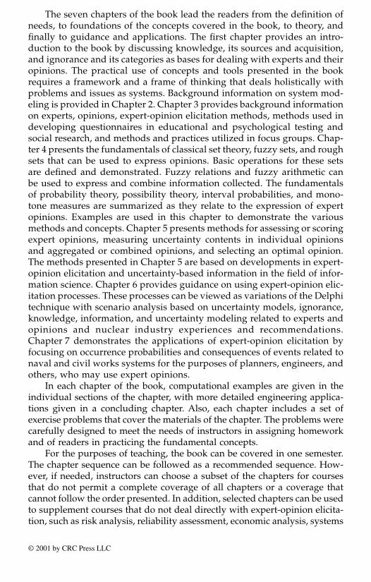
analysis, legal opinions, and social research courses. Chapters 1, 2, and 3can be covered concurrently. Chapter 4 builds on some of the materialcovered in Chapter 3. Chapter 5 builds on Chapters 3 and 4, and should becovered after completing Chapter 4. Chapter 6 provides guidance on usingexpert-opinion elicitation, and can be introduced after the preceding chap-ters. Chapter 7 provides applications. The book also contains an extensivereference section at its end. The accompanying schematic diagram illustratespossible sequences of these chapters in terms of their interdependencies.
Chapter 1Introduction
Chapter 2Systems
Chapter 3ElicitationMethods
Chapter 4ExpressingOpinions
Chapter 5Aggregating
Opinions
Chapter 6Guidance
Chapter 7Applications
Bibliography
© 2001 by CRC Press LLC

Acknowledgments
This book was developed over several years and draws on my experiencesin teaching courses related to risk analysis, uncertainty modeling and anal-ysis, probability and statistics, numerical methods and mathematics, reliabil-ity assessment, and decision analysis. Drafts of most sections of the bookwere tested in several courses at the University of Maryland, College Park,for about three years before its publication. This testing period has provedto be a very valuable tool in establishing its contents and the final formatand structure.
I was very fortunate to receive the direct and indirect help from manyindividuals, over many years, that greatly affected this book. Students whotook courses and used portions of this book provided me with great insighton how to effectively communicate various theoretical concepts. Also, stu-dents’ research projects and my interaction with them stimulated the gen-eration of various examples. The students who took courses on structuralreliability, risk analysis, and mathematical methods in civil engineering inthe 1990s contributed to this endeavor. Their feedback was very helpful andgreatly contributed to the final product. Also, comments provided by M. Al-Fadhala, I. Assakkaf, M. Kaminskiy, and R. Wlicox on selected chapters aregreatly appreciated.
I was fortunate to organize the International Symposia on UncertaintyModeling and Analysis in 1990, 1993, and 1995. These symposia were tre-mendously useful, as they provided me with rewarding opportunities tomeet, interact, and learn from researchers and scientists from more than 35countries, including most notably Professors D. Blockley, C.B. Brown, H.Furuta, M. Gupta, A. Haldar, L. Kanal, A. Kaufmann, G.J. Klir, R.R. Yager,J.T.P. Yao, L.A. Zadeh, H.G. Zimmerman.
The reviewers’ comments that were provided by the publisher were usedto improve the book to meet the needs of readers and enhance the educa-tional process. The input from the publisher and the book reviewers is greatlyappreciated.
The financial support that I received from the U.S. Navy, Coast Guard,Army Corps of Engineers, National Science Foundation, and the AmericanSociety of Mechanical Engineers over more than 15 years has contributedgreatly to this book by providing me with a wealth of information andideas for formalizing the theory, applications, and guidance. In particular,
© 2001 by CRC Press LLC

I acknowledge the opportunity and support provided by A. Ang, R. Art,K. Balkey, J. Beach, P. Capple, J. Crisp, D. Dressler, M. Firebaugh, J. Foster,Z. Karaszewski, D. Moser, G. Remmers, T. Shugar, S. Taylor, S. Wehr, andG. White.
The University of Maryland at College Park has provided me with theplatform, support, and freedom that made such a project possible. It hasalways provided me with a medium for creativity and excellence. I amindebted all my life for what the University of Maryland at College Park,especially the A. James Clark School of Engineering and the Department ofCivil and Environmental Engineering, has done for me. The students, staff,and my colleagues define this fine institution and its units.
Last but not least, I am boundlessly grateful to my family for acceptingmy absences, sometimes physical and sometimes mental, as I worked onprojects related to this book and its pages, for making it possible, and formaking my days worthwhile. I also greatly appreciate the boundless supportof my parents, brothers, and sisters: Thuraya, Mohammed, Saleh, Naser,Nidal, Intisar, Jamilah, and Mai. Finally, one individual who has acceptedmy preoccupation with the book and absence, kept our life on track, andfilled our life with treasures — or all of that, thanks to my wife, Deena; noneof this would be possible without her.
I invite users of the book to send any comments on the book to the e-mail address [email protected]. These comments will be used in devel-oping future editions of the book. Also, I invite users of the book to visit theweb site of the Center for Technology and Systems Management at theUniversity of Maryland, College Park, to find information posted on variousprojects and publications that can be related to expert-opinion elicitation.The URL is http://ctsm.umd.edu.
Bilal M. Ayyub
© 2001 by CRC Press LLC
About the author
Bilal M. Ayyub is a professor of civil and environmental engineering at theUniversity of Maryland (College Park) and the General Director of theCenter for Technology and Systems Management. He is also a researcherand consultant in the areas of structural engineering, systems engineering,uncertainty modeling and analysis, reliability and risk analysis, and appli-cations related to civil, marine, and mechanical systems. He completed hisB.S. degree in civil engineering in 1980, and completed both the M.S. (1981)and Ph.D. (1983) degrees in civil engineering at the Georgia Institute ofTechnology. He has performed several research projects that were fundedby the U.S. National Science Foundation, Coast Guard, Navy, Army Corpsof Engineers, Maryland State Highway Administration, American Societyof Mechanical Engineers, and several engineering companies. Dr. Ayyubserved the engineering community in various capacities through societiesthat include ASNE, ASCE, ASME, SNAME, IEEE, and NAFIPS. He is afellow of ASCE, ASME, and SNAME, and life member of ASNE and USNI.He chaired the ASCE Committee on the Reliability of Offshore Structures,and currently chairs the SNAME panel on design philosophy and the ASNENaval Engineers Journal committee. He also was the General Chairman ofthe first, second and third International Symposia on Uncertainty Modelingand Analysis that were held in 1990, 1993, and 1995, and NAFIPS annualconference in 1995. He is the author and coauthor of approximately 300publications in journals, and conference proceedings, and reports. His pub-lications include several textbooks and edited books. Dr. Ayyub is the triplerecipient of the ASNE “Jimmie” Hamilton Award for the best papers in theNaval Engineers Journal in 1985, 1992, and 2000. Also, he received the ASCEaward for “Outstanding Research Oriented Paper” in the Journal of WaterResources Planning and Management for 1987, the ASCE Edmund FriedmanAward in 1989, and in 1997 the NAFIPS K.S. Fu Award for distinguishedservice and Walter L. Huber Research Prize. He is a registered ProfessionalEngineer (PE) with the state of Maryland. He is listed in Who’s Who inAmerica, and Who’s Who in the World.
© 2001 by CRC Press LLC

Books by Bilal M. Ayyub
Probability, Statistics and Reliability for Engineers, CRC Press, 1997, B.M. Ayyuband R. McCuen.
Numerical Methods for Engineers, Prentice Hall, New York, 1996, by B.M.Ayyub and R. McCuen.
Uncertainty Modeling and Analysis in Civil Engineering, CRC Press, 1998, byB.M. Ayyub (Editor).
Uncertainty Modeling in Vibration, Control, and Fuzzy Analysis of StructuralSystems, World Scientific, 1997, by B.M. Ayyub, A. Guran, and A. Haldar(Editors).
Uncertainty Analysis in Engineering and the Sciences: Fuzzy Logic, Statistics, andNeural Network Approach, Kluwer Academic Publisher, 1997, by B.M. Ayyuband M.M. Gupta (Editors).
Uncertainty Modeling in Finite Element, Fatigue, and Stability of Systems, WorldScientific, 1997, by A. Haldar, A. Guran, and B.M. Ayyub (Editors).
Uncertainty Modeling and Analysis: Theory and Applications, North-Holland-Elsevier Scientific Publishers, 1994, by B.M. Ayyub and M.M. Gupta(Editors).
Analysis and Management of Uncertainty: Theory and Applications, North-Holland-Elsevier Scientific Publishers, by B.M. Ayyub and M.M. Gupta(Editors).
© 2001 by CRC Press LLC

Contents
Chapter 1. Knowledge and ignorance1.1. Information abundance and ignorance1.2. The nature of knowledge
1.2.1. Basic terminology and definitions1.2.2. Absolute reality and absolute knowledge1.2.3. Historical developments and perspectives
1.2.3.1. The preSocratic period1.2.3.2. The Socratic period1.2.3.3. The Plato and Aristotle period1.2.3.4. The Hellenistic1.2.3.5. The Medieval1.2.3.6. The Renaissance1.2.3.7. The 17th century1.2.3.8. The 18th century1.2.3.9. The 19th century1.2.3.10. The 20th century
1.2.4. Knowledge, information, and opinions1.3. Cognition and cognitive science1.4. Time and its asymmetry1.5. Defining ignorance in the context of knowledge
1.5.1. Human knowledge and ignorance1.5.2. Classifying ignorance1.5.3. Ignorance hierarchy
1.6. Exercise problems
Chapter 2. Information-based system definition2.1. Introduction2.2. System definition models
2.2.1. Perspectives for system definition2.2.2. Requirements and work breakdown structure
2.2.2.1. Requirements analysis2.2.2.2. Work breakdown structure
2.2.3. Process modeling method2.2.3.1. System engineering process
© 2001 by CRC Press LLC
2.2.3.2. Lifecycle of engineering systems2.2.3.3. Technical maturity model
2.2.4. Black-box method2.2.5. State-based method2.2.6. Component integration method2.2.7. Decision analysis method
2.2.7.1. Decision variables2.2.7.2. Decision outcomes2.2.7.3. Associated probabilities and consequences2.2.7.4. Decision trees2.2.7.5. Influence diagrams
2.3. Hierarchical definitions of systems2.3.1. Introduction2.3.2. Knowledge and information hierarchy
2.3.2.1. Source systems2.3.2.2. Data systems2.3.2.3. Generative systems2.3.2.4. Structure systems2.3.2.5. Metasystems
2.4. Models for ignorance and uncertainty types2.4.1. Mathematical theories for ignorance types2.4.2. Information uncertainty in engineering systems
2.4.2.1. Abstraction and modeling of engineeringsystems
2.4.2.2. Ignorance and uncertainty in abstracted aspects of a system
2.4.2.3. Ignorance and uncertainty in nonabstracted aspects of a system
2.4.2.4. Ignorance due to unknown aspectsof a system
2.5. System complexity2.6. Exercise problems
Chapter 3. Experts, opinions, and elicitation methods3.1. Introduction3.2. Experts and expert opinions3.3. Historical background
3.3.1. Delphi method3.3.2. Scenario analysis
3.4. Scientific heuristics3.5. Rational consensus3.6. Elicitation methods
3.6.1. Indirect elicitation3.6.2. Direct method3.6.3. Parametric estimation
3.7. Standards for educational and psychological testing
© 2001 by CRC Press LLC
3.8. Methods of social research3.9. Focus groups3.10. Exercise problems
Chapter 4. Expressing and modeling expert opinions4.1. Introduction4.2. Set theory
4.2.1. Sets and events4.2.2. Fundamentals of classical set theory
4.2.2.1. Classifications of sets4.2.2.2. Subsets4.2.2.3. Membership (or characteristic) function4.2.2.4. Sample space and events4.2.2.5. Venn-Euler diagrams4.2.2.6. Basic operations on sets
4.2.3. Fundamentals of fuzzy sets and operations4.2.3.1. Membership (or characteristic) function4.2.3.2. Alpha-cut sets4.2.3.3. Fuzzy Venn-Euler diagrams4.2.3.4. Fuzzy numbers, intervals and arithmetic4.2.3.5. Operations on fuzzy sets4.2.3.6. Fuzzy relations4.2.3.7. Fuzzy functions
4.2.4. Fundamental of rough sets4.2.4.1. Rough set definitions4.2.4.2. Rough set operations4.2.4.3. Rough membership functions4.2.4.4. Rough functions
4.3. Monotone measures4.3.1. Definition of monotone measures4.3.2. Classifying monotone measures4.3.3. Evidence theory
4.3.3.1. Belief measure4.3.3.2. Plausibility measure4.3.3.3. Basic assignment
4.3.4. Probability theory4.3.4.1. Relationship between evidence theory and
probability theory4.3.4.2. Classical definitions of probability4.3.4.3. Linguistic probabilities4.3.4.4. Failure rates4.3.4.5. Central tendency measures4.3.4.6. Dispersion (or variability)4.3.4.7. Percentiles4.3.4.8. Statistical uncertainty4.3.4.9. Bayesian methods
© 2001 by CRC Press LLC

4.3.4.10. Interval probabilities4.3.4.11. Interval cumulative distribution functions4.3.4.12. Probability bounds
4.3.5. Possibility theory4.4. Exercise problems
Chapter 5. Consensus and aggregating expert opinions5.1. Introduction5.2. Methods of scoring of expert opinions
5.2.1. Self scoring5.2.2. Collective scoring
5.3. Uncertainty measures5.3.1. Types of uncertainty measures5.3.2. Nonspecificity measures5.3.3. Entropy-like measures
5.3.3.1. Shannon entropy for probability theory5.3.3.2. Discrepancy measure5.3.3.3. Entropy measures for evidence theory
5.3.4. Fuzziness measure5.3.5. Other measures
5.4. Combining expert opinions5.4.1. Consensus combination of opinions5.4.2. Percentiles for combining opinions5.4.3. Weighted combinations of opinions5.4.4. Uncertainty-based criteria for combining
expert opinions5.4.4.1. Minimum uncertainty criterion5.4.4.2. Maximum uncertainty criterion5.4.4.3. Uncertainty invariance criterion
5.4.5. Opinion aggregation using interval analysis and fuzzy arithmetic
5.4.6. Opinion aggregation using Dempster’s ruleof combination
5.4.7. Demonstrative examples of aggregatingexpert opinions5.4.7.1. Aggregation of expert opinions5.4.7.2. Failure classification
5.5. Exercise problems
Chapter 6. Guidance on expert-opinion elicitation6.1. Introduction and terminology
6.1.1. Theoretical bases6.1.2. Terminology
6.2. Classification of issues, study levels, experts, and processoutcomes
6.3. Process definition
© 2001 by CRC Press LLC
6.4. Need identification for expert-opinion elicitation6.5. Selection of study level and study leader6.6. Selection of peer reviewers and experts
6.6.1. Selection of peer reviewers6.6.2. Identification and selection of experts6.6.3. Items needed by experts and reviewers before the
expert-opinion elicitation meeting6.7. Identification, selection, and development of technical
issues6.8. Elicitation of opinions
6.8.1. Issue familiarization of experts6.8.2. Training of experts6.8.3. Elicitation and collection of opinions6.8.4. Aggregation and presentation of results6.8.5. Group interaction, discussion, and revision
by experts6.9. Documentation and communication6.10. Exercise problems
Chapter 7. Applications of expert-opinion elicitation7.1. Introduction7.2. Assessment of occurrence probabilities
7.2.1. Cargo elevators onboard ships7.2.1.1. Background7.2.1.2. Example issues and results
7.2.2. Navigation locks7.2.2.1. Background7.2.2.2. General description of lock operations7.2.2.3. Description of components7.2.2.4. Example issues and results
7.3. Economic consequences of floods7.3.1. Background7.3.2. The Feather River Basin
7.3.2.1. Levee failure and consequent flooding7.3.2.2. Flood characteristics7.3.2.3. Building characteristics7.3.2.4. Vehicle characteristics
7.3.3. Example issues and results7.3.3.1. Structural depth-damage relationships7.3.3.2. Content depth-damage relationships7.3.3.3. Content-to-structure value ratios7.3.3.4. Vehicle depth-damage relationship
Bibliography
© 2001 by CRC Press LLC

chapter one
Knowledge and ignorance
Contents
1.1. Information abundance and ignorance1.2. The nature of knowledge
1.2.1. Basic terminology and definitions1.2.2. Absolute reality and absolute knowledge1.2.3. Historical developments and perspectives
1.2.3.1. The preSocratic period1.2.3.2. The Socratic period1.2.3.3. The Plato and Aristotle period1.2.3.4. The Hellenistic period1.2.3.5. The Medieval period1.2.3.6. The Renaissance1.2.3.7. The 17th century1.2.3.8. The 18th century1.2.3.9. The 19th century
1.2.3.10. The 20th century1.2.4. Knowledge, information, and opinions
1.3. Cognition and cognitive science1.4. Time and its asymmetry1.5. Defining ignorance in the context of knowledge
1.5.1. Human knowledge and ignorance1.5.2. Classifying ignorance1.5.3. Ignorance hierarchy
1.6. Exercise Problems
1.1 Information abundance and ignoranceCitizens of modern information-based, industrial societies are becomingincreasingly aware of, and sensitive to, the harsh and discomforting realitythat information abundance does not necessarily give us certainty. Some-times it can lead to errors in decision-making with undesirable outcomes
© 2001 by CRC Press LLC

due to either overwhelming and confusing situations, or a sense of overcon-fidence leading to improper information use. The former situation can be anoutcome of the limited capacity of a human mind in some situations to dealwith complexity and information abundance; whereas the latter can be attrib-uted to a higher order of ignorance, called the ignorance of self-ignorance.
As our society advances in many scientific dimensions and invents newtechnologies, human knowledge is being expanded through observation,discovery, information gathering, and logic. Also, the access to newly gen-erated information is becoming easier than ever as a result of computers andthe Internet. We are entering an exciting era where electronic libraries, on-line databases, and information on every aspect of our civilization, such aspatents, engineering products, literature, mathematics, physics, medicine,philosophy, and public opinions will become a few mouse-clicks away. Inthis era, computers can generate even more information from abundantlyavailable online information. Society can act or react based on this informa-tion at the speed of its generation, creating sometimes nondesirable situa-tions, for example, price and/or political volatilities. There is a great needto assess uncertainties associated with information and to quantify our stateof knowledge and/or ignorance. The accuracy, quality, and incorrectness ofsuch information and knowledge incoherence are coming under focus byour philosophers, scientists, engineers, technologists, decision and policymakers, regulators and lawmakers, and our society as a whole. As a result,uncertainty and ignorance analyses are receiving a lot of attention by oursociety. We are moving from emphasizing the state of knowledge expansionand creation of information to a state that includes knowledge and informa-tion assessment by critically evaluating them in terms of relevance, com-pleteness, nondistortion, coherence, and other key measures.
Our society is becoming less forgiving of, and more demanding from,our knowledge base. Untimely processing and use of any available informa-tion, even if it might be inconclusive, is considered worse than a lack ofknowledge and ignorance. In 2000, the U.S. Congress and the Justice Depart-ment investigated Firestone and Ford Companies for allegedly knowingabout their defective tires, suspected of causing accidents claiming morethan 88 lives worldwide, without taking appropriate actions. The investiga-tion and news elevated the problem to the level of scandal because of thecompany’s inaction on available information, although the Firestone andFord Companies argued that test results conducted, after they knew abouta potential problem, were inconclusive. Such reasoning can easily be takenby our demanding society as a cover-up, causing a belligerent attitude thatis even worse than the perception of inaction by corporate executives.Although people have some control over the levels of technology-causedrisks to which they are exposed, governments and corporations need topursue risk reduction as a result of increasing demands by our society, whichgenerally entails a reduction of benefits, thus posing a serious dilemma.Policy makers and the public are required, with increasing frequency, tosubjectively weigh benefits against risks and assess associated uncertainties
© 2001 by CRC Press LLC

when making decisions. Further, lacking a systems or holistic approach,vulnerability exists for overpaying to reduce one set of risks that may intro-duce offsetting or larger risks of another kind.
The objective of this chapter is to discuss knowledge, its sources, andacquisition, as well as ignorance and its categories as bases for dealing withexperts and their opinions. The practical use of concepts and tools presentedin the book requires a framework and a frame of thinking that deals holis-tically with problems and issues as systems. Background information onsystem modeling is provided in Chapter 2.
1.2 The nature of knowledge1.2.1 Basic terminology and definitions
Philosophers have concerned themselves with the study of knowledge, truth,reality, and knowledge acquisition since the early days of Greece, includingThales (c. 585 BC), Anaximander (611–547 BC), and Anaximenes (c. 550 BC)who first proposed a rational explanation of the natural world and its pow-ers. This section provides a philosophical introduction to knowledge, epis-temology, their development, and related terminology.
Philosophy (philosophia) is a Greek term meaning love of wisdom. It dealswith the careful thought about the fundamental nature of the world, thegrounds for human knowledge, and the evaluation of human conduct. Phi-losophy, as an academic discipline, has chief branches that include logic,metaphysics, epistemology, and ethics. Selected terms related to knowledgeand epistemology are defined in Table 1.1.
Philosophers’ definitions of knowledge, its nature, and methods of acqui-sitions evolved over time, producing various schools of thought. In subse-quent sections, these developments are briefly summarized along a historicaltimeline referring only to what was subjectively assessed as primary depar-tures from previous schools. The new schools can be considered as newalternatives, since in some cases they could not invalidate previous ones.
1.2.2 Absolute reality and absolute knowledge
The absolute reality of things is investigated in a branch of philosophy calledmetaphysics that is concerned with providing a comprehensive account of themost general features of reality as a whole. The term metaphysics is believedto have originated in Rome about 70 BC by the Greek peripatetic philosopherAndronicus of Rhodes in his edition of the works of Aristotle (384–322 BC).
Metaphysics typically deals with issues related to the ultimate nature ofthings, identification of objects that actually exist, things that compose theuniverse, the ultimate reality, the nature of mind and substance, and themost general features of reality as a whole. On the other hand, epistemologyis a branch of philosophy that investigates the possibility, origins, nature,and extent of human knowledge. Metaphysics and epistemology are very
© 2001 by CRC Press LLC

closely linked and, at times, indistinguishable as the former speculates aboutthe nature of reality, and latter speculates about the knowledge of it. Meta-physics is often formulated in terms of three modes of reality — the imma-terial mind (or consciousness), the matter (or physical substance), and a highernature (one which transcends both mind and matter) — according to threespecific philosophical schools of thought: idealism, materialism, and tran-scendentalism, respectively.
Table 1.1 Selected Knowledge and Epistemology Terms
Term Definition
Philosophy The fundamental nature of the world, the grounds for human knowledge, and the evaluation of human conduct.
Epistemology A branch of philosophy that investigates the possibility, origins, nature, and extent of human knowledge.
Metaphysics
Ontology
Cosmology
Cosmogony
The investigation of ultimate reality. A branch of philosophy concerned with providing a comprehensive account of the most general features of reality as a whole, and the study of being as such. Questions about the existence and nature of minds, bodies, God, space, time, causality, unity, identity, and the world are all metaphysical issues.
A branch of metaphysics concerned with identifying, in the most general terms, the kinds of things that actually exist.
A branch of metaphysics concerned with the origin of the world.
A branch of metaphysics concerned with the evolution of the universe.
Ethics A branch of philosophy concerned with the evaluation of human conduct.
Aesthetics A branch of philosophy that studies beauty and taste, including their specific manifestations in the tragic, the comic, and the sublime; where beauty is the characteristic feature of things that arouse pleasure or delight, especially to the senses of a human observer, and sublime is the aesthetic feeling aroused by experiences too overwhelming (i.e., awe) in scale to be appreciated as beautiful by the senses.
Knowledge A body of propositions that meet the conditions of justified true belief.
Priori Knowledge derived from reason alone.Posteriori Knowledge gained from intuitions and experiences.Rationalism Inquiry based on priori principles, or knowledge based
on reason.Empiricism Inquiry based on posteriori principles, or knowledge
based on experience.
© 2001 by CRC Press LLC

Idealism is based on a theory of reality, derived from Plato’s Theory ofIdeas (427–347 BC) that attributes to consciousness, or the immaterial mind, aprimary role in the constitution of the world. Metaphysical idealism con-tends that reality is mind-dependent and that true knowledge of reality isgained by relying upon a spiritual or conscious source.
The school of materialism is based on the notion that all existence isresolvable into matter, or into an attribute or effect of matter. Accordingly,matter is the ultimate reality, and the phenomenon of consciousness isexplained by physiochemical changes in the nervous system. In metaphysics,materialism is the antithesis of idealism in which the supremacy of mind isaffirmed, and matter is characterized as an aspect or objectification of mind.The world is considered to be entirely mind-independent, composed onlyof physical objects and physical interactions. Extreme or absolute material-ism is known as materialistic monism, the theory that all reality is derivedfrom one substance. Modern materialism has been largely influenced by thetheory of evolution as described in subsequent sections.
Plato developed the school of transcendentalism by arguing for a higherreality (metaphysics) than that found in sense experience, and for a higherknowledge of reality (epistemology) than that achieved by human reason.Transcendentalism stems from the division of reality into a realm of spiritand a realm of matter. It affirms the existence of absolute goodness charac-terized as something beyond description and as knowable ultimately onlythrough intuition. Later, religious philosophers applied this concept of tran-scendence to divinity, maintaining that God can be neither described norunderstood in terms that are taken from human experience. This doctrinewas preserved and advanced by Muslim philosophers, such as Al-Kindi(800–873), Al-Farabi (870–950), Ibn Sina (980–1037), and Ibn Rushd(1128–1198), and adopted and used by Christian philosophers, such asAquinas (1224–1274) in the medieval period as described in subsequentsections.
Epistemology deals with issues such as the definition of knowledge andrelated concepts, the sources and criteria of knowledge, the kinds of knowl-edge possible and the degree to which each is certain, and the exact relationbetween the one who knows and the object known. Knowledge can be basedon priori, knowledge derived from reason alone, and posteriori, knowledgegained by reference to intuitions or the facts of experience. Epistemologycan be divided into rationalism, inquiry based on a priori principles —knowledge based on reason, and empiricism, inquiry based on a posterioriprinciples — knowledge based on experience.
Philosophical views on knowledge evolved over time. The subsequentsections summarize these views on knowledge and describe their evolutioninto contemporary schools. The presentation in these sections is drawn onthe works of selected philosophers who either had great influence or arerepresentatives of their respective periods. Solomon and Higgins (1996),Russell (1975), Popkin (2000), Durant (1991), and Honderich (1995) are
© 2001 by CRC Press LLC

recommended sources for additional details on any of the views presentedin these sections.
1.2.3 Historical developments and perspectives
1.2.3.1 The preSocratic periodThe preSocratic period includes Gorgias (483-378 BC), Heraclitus (535–475BC), and Empedocles (c. 450 BC). Gorgias argued that nothing exists andthat knowledge does not exist, nor could it be communicated to others if itexisted. Heraclitus defined wisdom not as the knowledge of many thingsbut as the clear knowledge of one thing only, and he believed in perfectknowledge given only to the Gods; however, a progress in knowledge ispossible for “men.” Empedocles distinguished between the world as pre-sented to our senses (kosmos aisthetos) and the intellectual world (kosmosnoetos). Table 1.2 provides a summary of these views.
1.2.3.2 The Socratic periodThe Socratic period includes Socrates (469–399 BC), Antisthenes (440-370 BC),and Euclid (430–360 BC). The works of Socrates are available only throughthe descriptions of other philosophers such as Antisthenes and Euclid.Socrates’ contribution to philosophy was essentially in ethics by his teachingconcepts such as justice, love, virtue, and self-knowledge. He believed thatall vice was the result of ignorance, and that knowledge was virtue. Socratestaught that every person has full knowledge of ultimate truth containedwithin the soul and needs only to be spurred to conscious reflection in orderto become aware of it. Socrates employed two forms of philosophical inquiry,induction and definition. He considered dialectic thinking to be the highestmethod of speculative thought. Antisthenes defined happiness as a branchof knowledge that could be taught, and once acquired could not be lost.Euclid stated that knowledge is virtue. If knowledge is virtue, it can thereforebe the knowledge only of the ultimate being. Table 1.3 provides a summaryof these views.
Table 1.2 Knowledge Views during the PreSocratics Period
Philosophers (Year) Nature of Knowledge
Gorgias (483–378 BC)
Heraclitus(535–475 BC)
Empedocles(c. 450 BC)
Stated that knowledge does not exit nor can be communicated if existed.
Maintained that wisdom is not the knowledge of many things; it is the clear knowledge of one thing only. Perfect knowledge is only given to the Gods, but a progress in knowledge is possible for “men.”
Distinguished between the world as presented to our senses (kosmos aisthetos) and the intellectual world (kosmos noetos).
© 2001 by CRC Press LLC

1.2.3.3 The Plato and Aristotle periodThe Plato and Aristotle period includes Protagoras (485-415 BC), Plato(427–347 BC, see Figure 1.1), and Aristotle (384–322 BC, see Figure 1.2).Protagoras defined knowledge to be relative since it is based on individualexperiences.
Plato’s answer to Socrates’ question, what makes a kind of thing thekind of thing it is, was that the form itself does so, and that the form issomething different from the thing or object, having an eternal existence ofits own. Thus, beautiful things are beautiful because they partake of beautyitself, and just acts are just insofar as they partake of justice itself, and soforth. The highest form was that of the good. Most of Plato’s philosophy isconcerned with metaphysics as provided in the theory of reality. Accordingto this theory, reality or truth is provided by forms or ideas such as justiceitself. These forms constitute the basis for reality and exist separately fromthe objects that are abstracted by the human senses. Humans in turn describethese objects as pale copies of the forms. Plato stated that knowledge existsbased on unchanging and invisible forms or ideas. Objects that are sensedare imperfect copies of the pure forms. Genuine knowledge about theseforms can be achieved only by abstract reasoning through philosophy andmathematics. Like Socrates, Plato regarded ethics as the highest branch ofknowledge; he stressed the intellectual basis of virtue and identified virtuewith wisdom. Plato rejected empiricism, the claim that knowledge is derivedfrom sense experiences since propositions derived from sense experienceshave, at most, a degree of belief and are not certain. Plato’s theory of formswas intended to explain how one comes to know and also how things havecome to be as they are; i.e., the theory is both an epistemological (theory ofknowledge) and an ontological (theory of being) thesis.
The word Platonism refers both to the doctrines of Plato and to themanner or tradition of philosophizing that he founded. Often in philosophy,Platonism is virtually equivalent to idealism or intrinsicism since Plato wasthe first Western philosopher to claim that reality is fundamentally some-thing ideal or abstract and that knowledge largely consists of insight into orperception of the ideal. In common usage, the adjective Platonic refers to theideal; for example, Platonic love is the highest form of love that is nonsexualor nonphysical.
Plato recognized that knowledge is better than opinions. For someoneto know what piety is, she or he must know it through the form, which can
Table 1.3 Knowledge Views during the Socrates Period
Philosophers (Year) Nature of Knowledge
Antisthenes (440–370BC)
Euclid (430–360 BC)
Maintained that happiness is a branch of knowledge that could be taught, and that once acquired could not be lost.
Maintained that knowledge is virtue. If knowledge is virtue, it can only be the knowledge of the ultimate being.
© 2001 by CRC Press LLC

only be thought and not sensed. Thus knowledge belongs to an invisible,intangible, insensible world of the intellect, while in the visible, tangible,sensible world we have only opinions. The intelligible world is more realand true than the sensible world, as well as being more distinct.
Reality, truth, and distinctness can be made for both invisible and visibleworlds or realms. Within each realm, there is a further division. In the realmof the visible, there are real objects and their images, such as shadows andmirror images. These images give us the lowest grade or level of belief, mereconjectures. By seeing a shadow of an object, very little information aboutthe specific object is gained. Similarly, there is a division within the intelli-gible realm, between the forms themselves and images of the forms. Knowl-edge of the forms themselves through reason is the highest kind of knowl-edge, while knowledge of the images of the forms through understandingthe images is a lower form. Our opinions about the objects of the world aredeveloped through the use of the senses, by observation. Humans can
Figure 1.1 Bust of Plato. (©Archivo Iconografico, S.A./CORBIS. With permission.)
© 2001 by CRC Press LLC

observe what things tend to go together all the time and thus develop theopinion that those things belong together. Humans might try to understandobjects of the visible world by using senses, making assumptions, and explor-ing what follows from these interpretations and assumptions using logic.The use of assumptions can enable us to generate laws that explain whythings go together the way they do. For example, Newton assumed thatbodies in motion tend to stay in motion, and bodies at rest tend to stay atrest, unless some outside agency acts on them. This assumption about inertiahelped him generate further principles about motion, but it is not itselfproved. It can be treated as an unexamined assumption, in Plato’s terms. Thismethod of proceeding based on assumptions is not the best way possiblefor knowledge expansion since ideally it is preferred to use forms as basesfor explaining other things. The forms are not only what give us knowledge,but they also can be what give things their reality. The sun casts light uponthe earth, allowing us to see what is there, and it also supplies the energythrough which things grow and prosper. Accordingly, the form of the goodgives to the sensible world the reality it has.
The works of Plato formed the basis for Neoplatonism, founded by Ploti-nus (205–270), which greatly influenced medieval philosophers. Aristotlefollowed Plato as his student; however, Aristotle maintained that knowledgecan be derived from sense experiences, a departure from Plato’s thoughts.Knowledge can be gained either directly or indirectly by deduction usinglogic. For Aristotle, form and matter were inherent in all things and insep-arable. Aristotle rejected the Platonic doctrine that knowledge is innate andinsisted that it can be acquired only by generalization from experiences,emphasizing empiricism by stating that, “there is nothing in the intellect thatwas not first in the senses.” Table 1.4 provides a summary of the viewsduring this period.
Table 1.4 Knowledge Views during the Plato and Aristotle Periods
Philosophers (Year) Nature of Knowledge
Protagoras (485–415 BC)
Plato (427–347 BC)
Aristotle (384–322 BC)
Maintained that knowledge is relative since it is based on individual experiences
Maintained that knowledge can exist based on unchanging and invisible Forms or Ideas. Objects that are sensed are imperfect copies of the pure forms. Genuine knowledge about these forms can be achieved only by abstract reasoning through philosophy and mathematics.
Followed Plato, but maintained that knowledge is derived from sense experiences. Knowledge can be gained either directly or indirectly by deduction using logic.
© 2001 by CRC Press LLC

1.2.3.4 The Hellenistic periodThe Hellenistic period includes Epicurus (341–271 BC), Epictetus (55–135 BC),and Pyrrho (360–270 BC). Epicurus and Epictetus argued that philosophyshould be a means not an end. Pyrrho argued for skepticism in logic andphilosophy by denying the possibility of attaining any knowledge of realityapart from human perceptions. Table 1.5 provides a summary of these views.
1.2.3.5 The Medieval PeriodThe Medieval period can be characterized as an Islamic-Arabic period thatresulted in translating, preserving, commenting on, and providing Europewith the works of Greek philosophers. Also, the philosophers of this periodmaintained and strengthened the school of rationalism and laid the founda-tion of empiricism. The philosophers of this period were influenced by Plato,Aristotle, and Plotinus who founded Neoplatonism, a term first used byGerman philosophers in the 18th century to describe a perceived develop-ment in the history of Platonism. Plotinus (205–270) is generally recognizedas the founder of Neoplatonism. Plotinus’ principal assumptions can bestated crudely as follows:
Figure 1.2 Portrait of Aristotle (From ©Leonard de Selva/CORBIS. With permission.)
Table 1.5 Knowledge Views during the Hellenistic Period
Philosophers (Year) Nature of Knowledge
Epicurus (341–271 BC) & Epictetus (55–135 CE)
Pyrrho (360–270 BC)
Said philosophy is a means not an end.
Argued for skepticism in logic and philosophy.
© 2001 by CRC Press LLC

1. Truth exists and that it is the way the world exists in the mind or theintellect;
2. The awareness of the world as it exists in the intellect is knowledge;and
3. Two kinds of truth exist, contingent and necessary truth; for example,a contingent truth may be that ten coins are in a pocket, and anecessary truth is that four plus six equals ten.
Plotinus’ innovations in Platonism were developed in his essays, theEnneads, which comes from the Greek word for the number nine; the essaysare divided into nine groups. These groups cover ethical matters, naturalphilosophy, cosmology, the soul, intellect, knowledge, eternal truth, being,numbers, and the One. These innovations gave rise to Islamic Neoplatonism.
This period includes leading philosophers such as Al-Kindi (800–873),Al-Farabi (870–950), Ibn Sina (named Avicenna by the West, 980–1037), IbnRushd (named Averroes by the West, 1128–1198, see Figure 1.3), and Aquinas(1224–1274). Al-Kindi translated, preserved, and commented on Greek worksduring the Arabic civilization.
Figure 1.3 Ibn Rushd (named Averroes by the West, 1128-1198).
© 2001 by CRC Press LLC

Al-Farabi carried the thoughts of Aristotle and was named the SecondTeacher, Aristotle being the first. According to him, logic was divided intoIdea and Proof. Al-Farabi made use of the logical treatises of Aristotle andemployed arguments for the existence of God based upon those of Aristotle’smetaphysics. The arguments were designed to provide a rational foundationfor orthodox monotheism, and many of these arguments made their wayinto the Christian tradition later in the 13th century. Ibn Sina effectivelysynthesized Aristotelian, Neoplatonic, and Islamic thoughts. Ibn Rushd wasnamed the Commentator and the Philosopher. His primary work (Tuhafutal-Tuhafut translated from Arabic as The Incoherence of Limiting Rationalism)was critical of the works of medieval philosophers in limiting rationalismand moving towards faith and revelation. For example, Al-Ghazali(1058–1128) in his work Tuhafut al-Falasefah, translated from Arabic as theIncoherence of the Philosophers, argued for less rationalism and more faith. Thisdebate led to less rationalism in Islamic-Arabic thoughts and more of it inEuropean thought, preparing for modern philosophy and the renaissance ofEurope. Ibn Rushd attempted to overcome the contradictions between Aris-totelian philosophy and revealed religion by distinguishing between twoseparate systems of truth: a scientific body of truths based on reason, and areligious body of truths based on revelation. This is called the double-truthdoctrine, and influenced many Muslim, Jewish, and Christian philosophers.
Aquinas followed the schools of Plato and Aristotle and emphasizedreligious belief and faith. Following Neoplatonists, he considered the soul ahigher form of existence than the body, and taught that knowledge resultsfrom the contemplation of Platonic ideas that have been purified of bothsensation and imagery. He argued that the truths of natural science andphilosophy are discovered by reasoning from facts of experiences, and thetenets of revealed religion — the doctrine of the Trinity, the creation of theworld, and other articles of Christian dogma — are beyond rational com-prehension, although not inconsistent with reason, and must be accepted onfaith. Table 1.6 provides a summary of these views.
1.2.3.6 The RenaissanceThe Renaissance included Bacon (1561–1626), Galileo (1564–1642), Newton(1642–1727), and Montaigne (1533–1592). Bacon denounced reliance onauthority and verbal argument, criticized Aristotelian logic as useless for thediscovery of new laws, and formulated rules of inductive inference. Galileoexplained and defended the foundations of a thoroughly empirical view ofthe world and created the science of mechanics, which applied the principlesof geometry to the motions of bodies, and that relied heavily on experimen-tation and empirical thoughts. Newton applied mathematics to the study ofnature by formulating laws of universal gravitation and motion that explainhow objects move on Earth, as well as through the heavens. Montaignebelongs to the skepticism school with his motto “what do I know.” Table 1.7provides a summary of these views.
© 2001 by CRC Press LLC

1.2.3.7 The 17th centuryThe 17th century includes Descartes (1596–1650), Spinoza (1632–1677), andLocke (1632–1704). Descartes, the father of modern philosophy, identifiedrationalism, which is sometimes called Cartesian rationalism. Rationalism is asystem of thought that emphasizes the role of reason and priori principlesin obtaining knowledge; Descartes used the expression “I think, therefore Iam.” He also believed in the dualism of mind (thinking substance) and body(extended substance). Spinoza termed metaphysical (i.e., cosmological) con-cepts such as substance and mode, thought and extension, causation and paral-lelism, and essence and existence to reconcile concepts related to God,
Table 1.6 Knowledge Views during the Medieval Period
Philosophers (Year) Nature of Knowledge
Plotinus (205–270)
Al-Kindi (800–873)Al-Farabi (870–950)
Ibn Sina (980–1037)
Ibn Rushd (1128–1198)
Aquinas (1224–1274)
Plotinus’ principal assumptions can be stated crudely as follows: (1) truth exists and that it is the way the world exists in the mind or the intellect; (2) the awareness of the world as it exists in the intellect is knowledge; and (3) two kinds of truth exist, the contingent and the necessary; for example, a contingent truth is that ten coins are in a pocket, and a necessary truth is that four plus six equals ten.
Translated, preserved, and commented on Greek works.Carried the thoughts of Aristotle and was named the Second Teacher with Aristotle as the first. According to him logic was divided into Idea and Proof.
Synthesized Aristotelian, Neoplatonic, and Islamic thoughts.
Wrote a primary work (Tuhafut al-Tuhafut) critical of the works of medieval philosophers on limiting rationalismand moving to faith. Prepared for modern philosophy.
Followed the schools of Plato and Aristotle and added religious belief and faith.
Table 1.7 Knowledge Views during the Renaissance
Philosophers (Year) Nature of Knowledge
Bacon (1561–1626)
Galileo (1564–1642)
Newton (1642–1727)Montaigne(1533–1592).
Criticized Aristotelian logic as useless for the discovery of new laws; and formulated rules of inductive inference.
Explained and defended the foundations of a thoroughly empirical view of the world by creating the science of mechanics, which applied the principles of geometry to the motions of bodies.
Applied mathematics to the study of nature.Belongs to the skepticism school with his motto “what do I know.”
© 2001 by CRC Press LLC

substance, and nature. Locke identified empiricism as a doctrine affirmingthat all knowledge is based on experience, especially sense perceptions, andon posteriori principles. Empiricism denies the possibility of spontaneousideas or a priori thought. Locke distinguished two sources of experience:sensation-based knowledge of the external world and reflection-basedknowledge of the mind. Locke believed that human knowledge of externalobjects is always subject to the errors of the senses and concluded that onecannot have absolutely certain knowledge of the physical world. Table 1.8provides a summary of these views.
1.2.3.8 The 18th centuryThe 18th century includes leading philosophers such as Berkeley (1685–1753),Hume (1711–1776), and Kant (1724–1804). Berkeley is the founder of theschool of idealism. He agreed with Locke that knowledge comes throughideas, i.e., sensation of the mind, but he denied Locke’s belief that a distinc-tion can be made between ideas and objects. Berkeley held that matter cannotbe conceived to exist independent of the mind, and that the phenomena ofsense experiences can be explained only by supposing a deity that continu-ally evokes perception in the human mind. Extending Locke’s doubts aboutknowledge of the world outside the mind, Berkeley argued that no evidenceexists for the existence of such a world because the only things that one canobserve are one’s own sensations, and these are in the mind. Berkeley estab-lished the epistemological view phenomenalism, a theory of perception sug-gesting that matter can be analyzed in terms of sensations, preparing theway for the positivist movement in modern thought. Hume asserted that allmetaphysical things that cannot be directly perceived are meaningless. Hedivided all knowledge into two kinds: (1) relations of ideas, i.e., the knowledgefound in mathematics and logic, which is exact and certain but provides no
Table 1.8 Knowledge Views during the 17th Century
Philosophers (Year) Nature of Knowledge
Descartes (1596–1650)
Spinoza (1632–1677)
Locke (1632–1704)
As the father of modern philosophy, identifiedrationalism as a system of thought that emphasized the role of reason and priori principles in obtaining knowledge. He also believed in the dualism of mind (thinking substance) and body (extended substance).
Termed metaphysical (i.e., cosmological) concepts such as substance and mode, thought and extension, causation and parallelism, and essence and existence.
Identified empiricism as a doctrine that affirms that all knowledge is based on experience, especially sense perceptions, and on posteriori principles. Locke believed that human knowledge of external objects is always subject to the errors of the senses, and concluded that one cannot have absolutely certain knowledge of the physical world.
© 2001 by CRC Press LLC

information about the world; and (2) matters of fact, i.e., the knowledgederived from sense perceptions. Furthermore, he held that even the mostreliable laws of science might not always remain true. Kant provided acompromise between empiricism and rationalism by combining them. Hedistinguished between three types of knowledge: (1) an analytical priori,which is exact and certain, but also uninformative because it makes clearonly what is contained in definitions; (2) a synthetic posteriori, which conveysinformation about the world learned from experience but is subject to theerrors of the senses; and (3) a synthetic priori, which is discovered by pureintuition and is both exact and certain, for it expresses the necessary condi-tions that the mind imposes on all objects of experience. The 19th centuryphilosophers argued over the existence of the above third type of knowledge.Table 1.9 provides a summary of these views.
1.2.3.9 The 19th centuryThe 19th century includes leading philosophers such as Hegel (1770–1831),Comte (1798–1857), Marx (1818–1883) and Engels (1820–1895), and Nietzsche(1844–1900). Hegel claimed, as a rationalist, that absolutely certain knowledgeof reality can be obtained by equating the processes of thought, of nature,and of history. His absolute idealism was based on a dialectical process ofthesis, antithesis, and synthesis as cyclical and ongoing process; where athesis is any idea or a historical movement, an antithesis is a conflicting ideaor movement, and synthesis overcomes the conflict by reconciling a higherlevel of truth contained in both. Therefore, conflict and contradiction areregarded as necessary elements of truth, and truth is regarded as a processrather than a fixed state of things. He considered the Absolute Spirit to be thesum of all reality with reason as a master of the world, i.e., by stating that
Table 1.9 Knowledge Views during the 18th Century
Philosophers (Year) Nature of Knowledge
Berkeley (1685–1753)
Hume (1711–1776)
Kant (1724–1804)
Agreed with Locke that knowledge comes through ideas,i.e., sensation of the mind, but he denied Locke’s belief that a distinction can be made between ideas and objects.
Asserted that all metaphysical things that cannot be directly perceived are meaningless. Hume divided all knowledge into two kinds: relations of ideas, i.e., the knowledge found in mathematics and logic which is exact and certain but provides no information about the world, and matters of fact, i.e., the knowledge derived from sense perceptions. Furthermore, he held that even the most reliable laws of science might not always remain true.
Provided a compromise between empiricism and rationalism by combining both types, and distinguished three knowledge types: (1) an analytical priori, (2) a synthetic posteriori, and (3) a synthetic priori.
© 2001 by CRC Press LLC

“what is rational is real and what real is rational.” Comte brought attentionto the importance of sociology as a branch of knowledge and extended theprinciples of positivism, the notion that empirical sciences are the only ade-quate source of knowledge. Marx and Engels developed the philosophy ofdialectical materialism, based on the logic of Hegel, leading to social Darwinism,based on the theory of evolution developed by the British naturalist CharlesDarwin. According to social Darwinism, living systems compete in a strugglefor existence in which natural selection results in “survival of the fittest.”Marx and Engels derived from Hegel the belief that history unfolds accord-ing to dialectical laws and that social institutions are more concretely real thanphysical nature or the individual mind. Nietzsche concluded that traditionalphilosophy and religion are both erroneous and harmful, and that traditionalvalues (represented primarily by Christianity) had lost their power in thelives of individuals. He concluded that there are no rules for human life, noabsolute values, and no certainties on which to rely. Table 1.10 provides asummary of these views.
1.2.3.10 The 20th centuryThe 20th century includes leading philosophers such as Bradley (1846–1924),Royce (1855–1916), Peirce (1839–1914), Dewey (1859–1952), Husserl(1859–1938), Russell (1872–1970), Wittgenstein (1889–1951), and Austin(1911–1960). Bradley maintained that reality was a product of the mind ratherthan an object perceived by the senses. Like Hegel, he also maintained thatnothing is altogether real except the Absolute, the totality of everything whichtranscends contradiction. Everything else, such as religion, science, moralprecept, and even common sense, is contradictory. Royce believed in an
Table 1.10 Knowledge Views during the 19th Century
Philosophers (Year) Nature of Knowledge
Hegel (1770–1831)
Comte (1798–1857)
Marx (1818–1883) and Engels (1820–1895)
Nietzsche (1844–1900)
Claimed as a rationalist that absolutely certain knowledge of reality can be obtained by equating the processes of thought, of nature, and of history. His absolute idealism was based on a dialectical process of thesis, antithesis, and synthesis as cyclical and ongoing process.
Brought attention to the importance of sociology as a branch of knowledge and extended the principles of positivism, the notion that empirical sciences are the only adequate source of knowledge.
Developed the philosophy of dialectical materialism, based on the logic of Hegel.
Concluded that traditional philosophy and religion are both erroneous and harmful, and traditional values (represented primarily by Christianity) had lost their power in the lives of individuals. Therefore, there are no rules for human life, no absolute values, and no certainties on which to rely.
© 2001 by CRC Press LLC

absolute truth, and held that human thought and the external world wereunified. Peirce developed pragmatism as a theory of meaning, in particularthe meaning of concepts used in science. The only rational way to increaseknowledge was to form mental habits that would test ideas through obser-vation and experimentation leading to an evolutionary process of knowledgefor humanity and society, i.e., a perpetual state of progress. He believed thatthe truth of an idea or object could be measured only by empirical investi-gation of its usefulness. Pragmatists regarded all theories and institutions astentative hypotheses and solutions, and they believed that efforts to improvesociety must be geared toward problem solving in an ongoing process ofprogress. Pragmatism sought a middle ground between traditional meta-physical ideas about the nature of reality and the radical theories of nihilismand irrationalism which had become popular in Europe at that time. Theydid not believe that a single absolute idea of goodness or justice existed, butrather that these concepts were relative and depended on the context inwhich they were being discussed.
Pierce influenced a group of philosophers, called logical positivists, whoemphasized the importance of scientific verification, and rejected personalexperience as the basis of true knowledge. Dewey further developed prag-matism into a comprehensive system of thought that he called experimentalnaturalism, or instrumentalism. Naturalism regards human experience, intelli-gence, and social communities as ever-evolving mechanisms; thereforehuman beings could solve social problems using their experience and intel-ligence and through inquiry. He considered traditional ideas about knowl-edge and absolute reality or absolute truth to be incompatible with a Dar-winian world view of progress; therefore, they must be discarded or revised.
Husserl developed phenomenology as an elaborate procedure by whichone is said to be able to distinguish between the way things appear to beand the way one thinks they really are. Russell revived empiricism andexpanded to epistemology as a field. He attempted to explain all factualknowledge as constructed out of immediate experiences. Wittgenstein devel-oped logical positivism that maintained (1) only scientific knowledge exists,(2) any valid knowledge must be verifiable in experience, and (3) a lot ofprevious philosophy was neither true nor false, but literally meaningless. Inhis words, “philosophy is a battle against the bewitchment of our intelligenceby means of language.” He viewed philosophy as a linguistic analysis and“language games,” leading to his work Tractatus Logico-Philosophicus (1921)that asserted language is composed of complex propositions that can beanalyzed into less complex propositions until one arrives at simple or ele-mentary propositions. This view of decomposing complex language propo-sitions has a parallel in our view of the world to be composed of complexfacts that can be analyzed into less complex facts until one arrives at simple“picture atomic facts or states of affairs.” Wittgenstein’s picture theory ofmeaning required and built on atomic facts pictured by the elementary prop-ositions. Therefore, only propositions that picture facts are the propositionsof science that can be considered cognitively meaningful. Metaphysical,
© 2001 by CRC Press LLC

ethical, and theological statements, on the other hand, are not meaningfulassertions. Wittgenstein’s work influenced the work of Russell in developingthe theory of logical atomism.
Russell, Wittgenstein, and others formed the core of the Vienna Circlethat developed logical positivism in which philosophy is defined by its rolein clarification of meaning, not the discovery of new facts or the constructionof traditional metaphysics. They introduced strict principles of verifiabilityto reject as meaningless the nonempirical statements of metaphysics, theol-ogy, and ethics, and they regarded as meaningful only statements reportingempirical observations, taken together with the tautologies of logic andmathematics. Austin developed the speech-act theory, which states that manyutterances do not merely describe reality, but also have an effect on reality,insofar as they too are the performance of some act. Table 1.11 provides asummary of these views.
1.2.4 Knowledge, information, and opinions
Many disciplines of engineering and the sciences rely on the developmentand use of predictive models that in turn require knowledge and informationand sometimes subjective opinions of experts. Working definitions forknowledge, information, and opinions are needed for this purpose. In thissection, these definitions are provided with some limitations and discussionsof their uses.
Knowledge can be based on evolutionary epistemology using an evolution-ary model. It can be viewed to consist of two types, nonpropositional andpropositional knowledge. Nonpropositional knowledge can be further brokendown into know-how and concept knowledge, and familiarity knowledge (com-monly called object knowledge). Know-how and concept knowledge requiresomeone to know how to do a specific activity, function, procedure, etc.,such as riding a bicycle. Concept knowledge can be empirical in nature. Inevolutionary epistemology, know-how knowledge is viewed as a historicalantecedent to propositional knowledge. Object knowledge is based on adirect acquaintance with a person, place, or thing; for example, Mr. Smithknows the President of the United States. Propositional knowledge is basedon propositions that can be either true or false; for example, Mr. Smith knowsthat the Rockies are in North America (Sober 1991, and di Carlo 1998). Thisproposition can be expressed as
Mr. Smith knows that the Rockies are in North America (1-1a)
S knows P (1-1b)
where S is the subject, i.e., Mr. Smith, and P is the claim “the Rockies are inNorth America.” Epistemologists require the following three conditions formaking this claim in order to have a true proposition:
© 2001 by CRC Press LLC

Table 1.11 Knowledge Views during the 20th Century
Philosophers (Year) Nature of Knowledge
Bradley (1846–1924)
Royce (1855–1916)
Peirce (1839–1914)
Dewey (1859–1952)
Husserl (1859–1938)
Russell (1872–1970)
Wittgenstein (1889–1951)
Austin (1911–1960)
Maintained that reality was a product of the mind rather than an object perceived by the senses; like Hegel, nothing is altogether real except the Absolute, the totality of everything which transcends contradiction. Everything else, such as religion, science, moral precept, and even common sense, is contradictory.
Believed in an absolute truth and held that human thought and the external world were unified.
Developed pragmatism as a theory of meaning, in particular, the meaning of concepts used in science. The only rational way to increase knowledge was to form mental habits that would test ideas through observation and experimentation leading to an evolutionary process for humanity and society, i.e., a perpetual state of progress. He believed that the truth of an idea or object could only be measured by empirical investigation of its usefulness.
Further developed pragmatism into a comprehensive system of thought that he called experimental naturalism,or instrumentalism. Naturalism regards human experience, intelligence, and social communities as ever-evolving mechanisms; therefore human beings could solve social problems using their experience and intelligence, and through inquiry.
Developed phenomenology as an elaborate procedure by which one is said to be able to distinguish between the way things appear to be, and the way one thinks they really are.
Revived empiricism and expanded it to epistemology as a field.
Developed logical positivism that maintained that only scientific knowledge exists verifiable by experience. He viewed philosophy as a linguistic analysis and “language games” leading to his work Tractatus Logico-Philosophicus (1921) that asserted language, or the world, are composed of complex propositions, or facts, that can be analyzed into less complex propositions arriving at elementary propositions, or into less complex facts, arriving at simple “picture atomic facts or states of affairs,” respectively.
Developed the speech-act theory, in which language utterances might not describe reality and can have an effect on reality.
© 2001 by CRC Press LLC
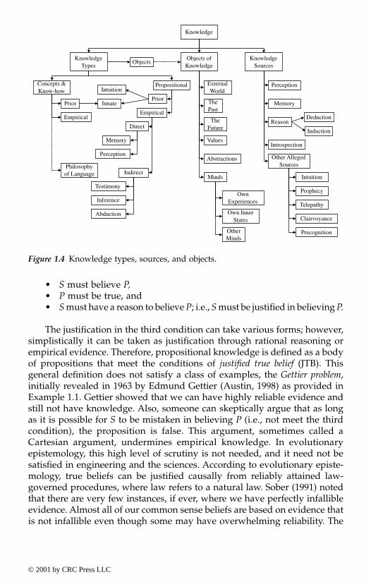
• S must believe P, • P must be true, and• S must have a reason to believe P; i.e., S must be justified in believing P.
The justification in the third condition can take various forms; however,simplistically it can be taken as justification through rational reasoning orempirical evidence. Therefore, propositional knowledge is defined as a bodyof propositions that meet the conditions of justified true belief (JTB). Thisgeneral definition does not satisfy a class of examples, the Gettier problem,initially revealed in 1963 by Edmund Gettier (Austin, 1998) as provided inExample 1.1. Gettier showed that we can have highly reliable evidence andstill not have knowledge. Also, someone can skeptically argue that as longas it is possible for S to be mistaken in believing P (i.e., not meet the thirdcondition), the proposition is false. This argument, sometimes called aCartesian argument, undermines empirical knowledge. In evolutionaryepistemology, this high level of scrutiny is not needed, and it need not besatisfied in engineering and the sciences. According to evolutionary episte-mology, true beliefs can be justified causally from reliably attained law-governed procedures, where law refers to a natural law. Sober (1991) notedthat there are very few instances, if ever, where we have perfectly infallibleevidence. Almost all of our common sense beliefs are based on evidence thatis not infallible even though some may have overwhelming reliability. The
Figure 1.4 Knowledge types, sources, and objects.
Knowledge
KnowledgeSources
KnowledgeTypes
Objects ofKnowledge
Objects
Concepts &Know-how
Propositional ExternalWorld
ThePast
TheFuture
Values
Abstractions
Minds
Perception
Memory
Reason
Introspection
Other AllegedSources
Intuition
OwnExperiences
Own InnerStates
OtherMinds
Telepathy
Precognition
Clairvoyance
Prophecy
Deduction
Induction
Prior
Empirical
Philosophyof Language
InnatePrior
Empirical
Intuition
Direct
Indirect
Memory
Perception
Testimony
Inference
Abduction
© 2001 by CRC Press LLC

presence of a small doubt in meeting the justification condition does notmake our evidence infallible but only reliable. Evidence reliability and infal-libility arguments form the basis of the reliability theory of knowledge. Figure1.4 shows a breakdown of knowledge by types, sources, and objects thatwas based on a summary provided by Honderich (1995).
In engineering and the sciences, knowledge can be defined as a body ofJTB, such as, laws, models, objects, concepts, know-how, processes, andprinciples, acquired by humans about a system of interest, where the justi-fication condition can be met based on the reliability theory of knowledge.The most basic knowledge category is cognitive knowledge (episteme) thatcan be acquired by human senses. The next level is based on correct reason-ing from hypotheses such as mathematics (dianoi). The third category movesus from intellectual categories to categories that are based on the realm ofappearances and deception and are based on propositions. This third cate-gory is belief (pistis — the Greek word for faith, denoting intellectual and/oremotional acceptance of a proposition). It is followed by conjecture (eikasia)in which knowledge is based on inference, theorization, or prediction basedon incomplete or reliable evidences. The four categories are shown inFigure 1.5 and also define the knowledge box in Figure 1.6. These categoriesconstitute the human cognition of human knowledge that might be differentfrom a future state of knowledge achieved by an evolutionary process, asshown in Figure 1.6. The pistis and eikasia categories are based on expertjudgment and opinions regarding system issues of interest. Although thepistis and eikasia knowledge categories might by marred with uncertainty,they are a certainty sought after in many engineering disciplines and thesciences, especially by decision and policy makers.
Information can be defined as sensed objects, things, places, processes,and information and knowledge communicated by language and multime-dia. Information can be viewed as a preprocessed input to our intellectsystem of cognition, and as knowledge acquisition and creation. It can leadto knowledge through investigation, study, and reflection. However, knowl-edge and information about the system might not constitute the eventualevolutionary knowledge state about the system as a result of not meetingthe justification condition in JTB or the ongoing evolutionary process or both.Knowledge is defined in the context of the humankind, evolution, languageand communication methods, and social and economic dialectic processes;it cannot be removed from them. As a result, knowledge would always reflectthe imperfect and evolutionary nature of humans, which is attributed to theirreliance on their senses for information acquisition; their dialectic processes;and their mind for extrapolation, creativity, reflection, and imagination, withassociated biases as a result of preconceived notions due to time asymmetry,specialization, and other factors. An important dimension in defining thestate of knowledge and truth about a system is nonknowledge or ignorance.
Opinions rendered by experts, that are based on information and existingknowledge, can be defined as preliminary propositions with claims that arenot fully justified or that are justified with adequate reliability but are not
© 2001 by CRC Press LLC

necessarily infallible. Expert opinions are seeds of propositional knowledgethat do not meet one or more of the conditions required by the JTB and thereliability theory of knowledge. They are valuable as they might lead toknowledge expansion, but decisions based on them sometimes might berisky propositions, since their preliminary nature means they might beproven false by others or in the future.
The relationships among knowledge, information, opinions, and evolu-tionary epistemology are schematically shown in Figure 1.5. The dialecticprocesses include communication methods such as languages, visual andaudio formats, and other forms. Also, they include economic, class, schoolsof thought, political and social dialectic processes within peers, groups,colonies, societies, and the world.
Example 1.1. A Gettier problem: a Ferrari owner or not
Knowledge was defined as accumulations of justified true beliefs (JTB). Thisgeneral definition does not satisfy any of a class of examples known collec-tively as the Gettier problem, initially revealed in 1963 by Edmund Gettier(Austin, 1998). For example, a teacher has two students, Mr. Nothavit andMr. Havit, in her class. Mr. Nothavit seems to be the proud owner of anexpensive car (a Ferrari). Mr. Nothavit says he owns one, drives one around,and has papers that state that he owns the car, but he does not actually owna Ferrari. On the basis of this evidence, the teacher concludes that the prop-osition “someone in her class owns a Ferrari” is true. This proposition is trueenough, but only because Mr. Havit, who shows no signs of Ferrari owner-ship, secretly owns one. Therefore, it seems that the three conditions (truth,justification, and belief) of knowledge have been met, but that there is noknowledge. So it is true that a Ferrari owner is a member of her class, theteacher accepts that it is true, and she is completely justified in so acceptingthat he is.
1.3 Cognition and cognitive scienceCognition can be defined as mental processes of receiving and processinginformation for knowledge creation and behavioral actions. Cognitive sci-ence is the interdisciplinary study of mind and intelligence (Stillings, 1995).Cognitive science deals with philosophy, psychology, artificial intelligence,neuroscience, linguistics, and anthropology. The intellectual origins of cog-nitive science started in the mid-1950s when researchers in several fieldsused complex representations and computational procedures to developtheories on how the mind works.
The origin of cognitive science can be taken as the theory of knowledgeand the theory of reality of the ancient Greeks, when philosophers such asPlato and Aristotle tried to explain the nature of human knowledge. Thestudy of mind remained the province of philosophy until the nineteenthcentury, when experimental psychology was developed by Wilhelm Wundt
© 2001 by CRC Press LLC

Figure 1.5 Knowledge categories and sources.
Figure 1.6 Knowledge, information, opinions, and evolutionary epistemology.
Cognitive knowledge that includesknow-how and object knowledge ( Episteme)
Propositional knowledge based onconjecture (Eikasia)
Propositional knowledge based onbelief (Pistis)
Correct reasoning from hypothesessuch as mathematics and logic ( Dianoi)
Bel
ong
to R
ealm
of
App
eara
nces
and
Dec
eptio
n
Human cognition that leadsto knowledge
Bel
ong
to R
ealm
of
App
eara
nces
and
Dec
eptio
n
Req
uire
Int
elle
ctua
lT
rain
ing
Req
uire
Int
elle
ctua
lT
rain
ing
Information:Sensed objects, things,places, processes, and
communicated informationand knowledge by language
and multi-media.
Opinion 1
Opinion n
Opinion 2
Dialecticalprocess
::
Knowledge:A body of justified true
beliefs (JTB), such as laws,models, objects, processes,and principles, acquired byhumankind about a system
of interest.
Test and Use ofKnowledge:
Study, investigation,utilization, and reflection on
the state of knowledge.
Evolution
Evolution
Evolution
© 2001 by CRC Press LLC

and his students by initiating laboratory methods for studying systematicallymental operations. A few decades later, experimental psychology becamedominated by behaviorism by which the existence of the mind was virtuallydenied. Behaviorists, such as J. B. Watson, argued that psychology shouldrestrict itself to examining the relation among observable stimuli and observ-able behavioral responses and should not deal with consciousness and mentalrepresentations. The intellectual landscape began to change dramatically in1956, when George Miller summarized numerous studies showing that thecapacity of human thinking is limited, with short-term memory, for example,limited to around seven items. He proposed that humans compensate formemory limitations through their ability to recode information into chunksand mental representations that require mental procedures for encoding anddecoding the information. Although at this time primitive computers hadbeen around for only a few years, pioneers such as John McCarthy, MarvinMinsky, Allen Newell, and Herbert Simon were founding the field of artificialintelligence. Moreover, Noam Chomsky rejected behaviorist assumptionsabout language as a learned habit and proposed instead to explain languagecomprehension in terms of mental grammars consisting of rules.
Cognitive science is based on a central hypothesis that thinking can bestbe understood in terms of representational structures in the mind and com-putational procedures that operate on those structures (Johnson-Laird, 1988).The nature of the representations and computations that constitute thinkingare not fully understood. The central hypothesis is general enough to encom-pass the current range of thinking in cognitive science, including connec-tionist theories which model thinking using artificial neural networks. Thishypothesis assumes that the mind has mental representations analogous tocomputer data structures, and computational procedures similar to compu-tational algorithms. The mind is considered to contain such mental repre-sentations as logical propositions, rules, concepts, images, and analogies. Ituses mental procedures such as deduction, search, matching, rotating, andretrieval for interpretation, generation of knowledge, and decision making.The dominant mind-computer analogy in cognitive science has taken on anovel twist from the use of another analog — the brain. Cognitive sciencethen works with a complex 3-way analogy among the mind, brain, andcomputers. Connectionists have proposed a brain-like structure that usesneurons and their connections as inspirations for data structures, and neuronfiring and spreading activation as inspirations for algorithms. There is nota single computational model for the mind, since different kinds of comput-ers and programming approaches suggest different ways in which the mindmight work, ranging from serial processors, such as the commonly usedcomputers that perform one instruction at a time, to parallel processors, suchas some recently developed computers that are capable of doing many oper-ations at once.
Cognitive science claims that the human mind works by representationand computation using empirical conjecture. Although the computational-representational approach to cognitive science has been successful in
© 2001 by CRC Press LLC

explaining many aspects of human problem solving, learning, and languageuse, some philosophical critics argue that it is fundamentally flawed becauseof the following limitations (Thagard, 1996, and Von Eckardt, 1993):
• Emotions: Cognitive science neglects the important role of emotionsin human thinking.
• Consciousness: Cognitive science ignores the importance of con-sciousness in human thinking.
• Physical environments: Cognitive science disregards the significantrole of physical environments on human thinking.
• Social factors: Human thought is inherently social and has to dealwith various dialectic processes in ways that cognitive scienceignores.
• Dynamical nature: The mind is a dynamical system, not a computa-tional system.
• Quantum nature: Researchers argue that human thinking cannot becomputational in the standard sense, so the brain must operate dif-ferently, perhaps as a quantum computer.
These open issues need to be considered by scientists and philosophersin developing new cognitive theories and a better understanding of how thehuman mind works.
1.4 Time and its asymmetry Time and its asymmetry are crucial in defining knowledge and ignorance(Horwich, 1987). Kurt Gödel speculated in a theory, which is consistent withthe General Theory of Relativity, that time flows from the past to the future,passing through the present, and allows for “time travel” to the past. How-ever, we can reliably claim, based on our current technology and knowledgebase, that time as a phenomenon has a unidirectional flow. Time can beviewed as a one-dimensional continuum of instants with temporally occur-ring events. The present (or now) is a gliding index that moves in a unidi-rectional form from the past to the future. “It is as if we were floating on ariver, carried by the current, past the manifold events which are spread outtimelessly on the bank,” said Plato.
Engineers and scientists are practitioners and specialists who often tryto make statements about the future. However, Aristotle asserted that con-tingent statements about the future have no truth value, unlike statementsmade about the past and present which are determinably either true or false.Events of interest can be viewed to progress in time tree-like, with fixedbranches of the past and forming branches of the present. However, thefuture branches manifold undetermined possibilities. Many scientific andengineering laws and principles display temporal irreversibility, such asthermodynamic system changes and chemical reactions. Therefore, they canbe viewed as time-asymmetric system changes and transitions. In addition,there are many physical processes that do not have temporal inverses.
© 2001 by CRC Press LLC
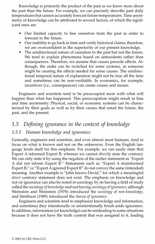
Knowledge is primarily the product of the past as we know more aboutthe past than the future. For example, we can precisely describe past dailytemperatures but cannot accurately forecast future temperatures. Time asym-metry of knowledge can be attributed to several factors, of which the signif-icant ones are
• Our limited capacity to free ourselves from the past in order toforecast in the future.
• Our inability to go back in time and verify historical claims; therefore,we are overconfident in the superiority of our present knowledge.
• The unidirectional nature of causation to the past but not the future.We tend to explain phenomena based on antecedents rather thanconsequences. Therefore, we assume that causes precede effects. Al-though, the order can be switched for some systems, as someonemight be creating the effects needed for some causes. The unidirec-tional temporal nature of explanation might not be true all the timeand sometimes can be non-verifiable. In economics, for example,incentives (i.e., consequences) can create causes and means.
Engineers and scientists tend to be preoccupied more with what willhappen than what has happened. This preoccupation might result in biasand time asymmetry. Physical, social, or economic systems can be charac-terized by their goals as well as by their causes that entail the future, thepast, and the present.
1.5 Defining ignorance in the context of knowledge1.5.1 Human knowledge and ignorance
Generally, engineers and scientists, and even almost most humans, tend tofocus on what is known and not on the unknowns. Even the English lan-guage lends itself for this emphasis. For example, we can easily state thatExpert A informed Expert B, whereas we cannot directly state the contrary.We can only state it by using the negation of the earlier statement as “ExpertA did not inform Expert B.” Statements such as “Expert A misinformedExpert B,” or “Expert A ignored Expert B” do not convey the same (intended)meaning. Another example is “John knows David,” for which a meaningfuldirect contrary statement does not exist. The emphasis on knowledge andnot on ignorance can also be noted in sociology by its having a field of studycalled the sociology of knowledge and not having sociology of ignorance, althoughWeinstein and Weinstein (1978) introduced the sociology of non-knowledge,and Smithson (1985) introduced the theory of ignorance.
Engineers and scientists tend to emphasize knowledge and information,and sometimes they intentionally or unintentionally brush aside ignorance.In addition, information (or knowledge) can be misleading in some situationsbecause it does not have the truth content that was assigned to it, leading
© 2001 by CRC Press LLC
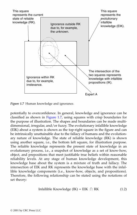
potentially to overconfidence. In general, knowledge and ignorance can beclassified as shown in Figure 1.7, using squares with crisp boundaries forthe purpose of illustration. The shapes and boundaries can be made multi-dimensional, irregular, and/or fuzzy. The evolutionary infallible knowledge(EIK) about a system is shown as the top-right square in the figure and canbe intrinsically unattainable due to the fallacy of humans and the evolution-ary nature of knowledge. The state of reliable knowledge (RK) is shownusing another square, i.e., the bottom left square, for illustration purpose.The reliable knowledge represents the present state of knowledge in anevolutionary process, i.e., a snapshot of knowledge as a set of know-how,object, and prepositions that meet justifiable true beliefs within reasonablereliability levels. At any stage of human knowledge development, thisknowledge base about the system is a mixture of truth and fallacy. Theintersection of EIK and RK represents the knowledge base with the infal-lible knowledge components (i.e., know-how, objects, and propositions).Therefore, the following relationship can be stated using the notations ofset theory:
Infallible Knowledge (IK) = EIK RK (1.2)
Figure 1.7 Human knowledge and ignorance.
This squarerepresents theevolutionaryinfallibleknowledge (EIK).
The intersection of thetwo squares representsknowledge with infalliblepropositions (IK).
Ignorance within RKdue to, for example,irrelevance.
This squarerepresents the currentstate of reliableknowledge (RK). Ignorance outside RK
due to, for example,the unknown.
Expert A
I
© 2001 by CRC Press LLC
where means intersection. Infallible knowledge is defined as knowl-edge that can survive the dialectic processes of humans and societies andthat passes the test of time and use. This infallible knowledge can be sche-matically defined by the intersection of these two squares of EIK and RK.Based on this representation, two primary types of ignorance can be identi-fied: (1) ignorance within the knowledge base RK due to factors such asirrelevance, and (2) ignorance outside the knowledge base due to unknownobjects, interactions, laws, dynamics, and know-how.
Expert A of some knowledge about the system can be represented asshown in Figure 1.7, using ellipses for illustrative purposes. Three types ofellipses can be identified: (1) a subset of the evolutionary infallible knowledge(EIK) that the expert has learned, captured, and/or created, (2) self-perceivedknowledge by the expert, and (3) perception by others of the expert’s knowl-edge. The EIK of the expert might be smaller than the self-perceived knowl-edge by the expert, and the difference between the two types is a measure ofoverconfidence that can be partially related to the expert’s ego. Ideally, thethree ellipses should be the same, but commonly they are not. They are greatlyaffected by communication skills of experts and their successes in dialecticprocesses that with time might lead to evolutionary knowledge marginaladvances or quantum leaps. Also, their relative sizes and positions withinthe infallible knowledge (IK) base are unknown. It can be noted from Figure1.7 that the expert’s knowledge can extend beyond the reliable knowledgebase into the EIK area as a result of creativity and imagination by the expert.Therefore, the intersection of the expert’s knowledge with the ignorance spaceoutside the knowledge base can be viewed as a measure of creativity andimagination. Another expert (i.e., Expert B) would have her/his own ellipsesthat might overlap with the ellipses of Expert A and might overlap with otherregions by varying magnitudes.
1.5.2 Classifying Ignorance
The state of ignorance for a person or society can be unintentional or delib-erate due to an erroneous cognition state and not knowing relevant infor-mation, or ignoring information and deliberate inattention to something forvarious reasons, such as limited resources or cultural opposition, respec-tively. The latter type is a state of conscious ignorance which is not intentional,and once it is recognized evolutionary species try to correct that state forsurvival reasons, with varying levels of success. The former ignorance typebelongs to the blind ignorance category. Therefore, ignoring means that some-one can either unconsciously or deliberately refuse to acknowledge or regard,or leave out an account or consideration for relevant information (di Carlo,1998). These two states should be treated in developing a hierarchal break-down of ignorance.
Using the concepts and definitions from evolutionary knowledge andepistemology, ignorance can be classified based on the three knowledgesources as follows:
I
© 2001 by CRC Press LLC
• Know-how ignorance can be related to the lack of know-how knowl-edge or the having of erroneous know-how knowledge. Know-howknowledge requires someone to know how to do a specific activity,function, procedure, etc., such as riding a bicycle.
• Object ignorance can be related to the lack of object knowledge or thehaving of erroneous object knowledge. Object knowledge is basedon a direct acquaintance with a person, place or thing; for example,Mr. Smith knows the President of the United States.
• Propositional ignorance can be related to the lack of propositionalknowledge or the having of erroneous propositional knowledge.Propositional knowledge is based on propositions that can be eithertrue or false; for example, Mr. Smith knows that the Rockies are inNorth America.
The above three ignorance types can be cross-classified against twopossible states for a knowledge agent, such as a person, of knowing theirstate of ignorance. These two states are
• Nonreflective (or blind) state: The person does not know of self-igno-rance, a case of ignorance of ignorance.
• Reflective state: The person knows and recognizes self-ignorance.Smithson (1985) termed this type of ignorance conscious ignorance,and the blind ignorance was termed meta-ignorance. As a result, insome cases the person might formulate a proposition but still beignorant of the existence of a proof or disproof. A knowledge agent’sresponse to reflective ignorance can be either passive acceptance ora guided attempt to remedy one’s ignorance that can lead to fourpossible outcomes: (1) a successful remedy that is recognized by theknowledge agent to be a success, leading to fulfillment; (2) a success-ful remedy that is not recognized by the knowledge agent to be asuccess, leading to searching for a new remedy; (3) a failed remedythat is recognized by the knowledge agent to be a failure, leading tosearching for a new remedy; and (4) a failed remedy that is recog-nized by the knowledge agent to be a success, leading to blind igno-rance, such as ignoratio elenchi, i.e., ignorance of refutation or missingthe point or irrelevant conclusion.
The cross classification of ignorance is shown in Figure 1.8 in two pos-sible forms that can be used interchangeably. Although the blind state doesnot feed directly into the evolutionary process for knowledge, it representsa becoming knowledge reserve. The reflective state has a survival value toevolutionary species; otherwise it can be argued that it never would haveflourished (Campbell, 1974). Ignorance emerges as a lack of knowledgerelative to a particular perspective from which such gaps emerge. Accord-ingly, the accumulation of beliefs and the emergence of ignorance constitutea dynamic process resulting in old ideas perishing and new ones flourishing
© 2001 by CRC Press LLC
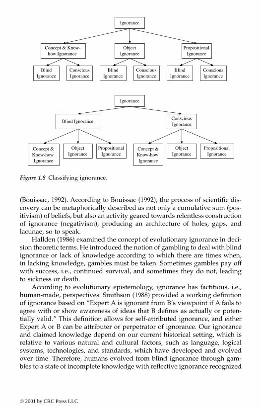
(Bouissac, 1992). According to Bouissac (1992), the process of scientific dis-covery can be metaphorically described as not only a cumulative sum (pos-itivism) of beliefs, but also an activity geared towards relentless constructionof ignorance (negativism), producing an architecture of holes, gaps, andlacunae, so to speak.
Hallden (1986) examined the concept of evolutionary ignorance in deci-sion theoretic terms. He introduced the notion of gambling to deal with blindignorance or lack of knowledge according to which there are times when,in lacking knowledge, gambles must be taken. Sometimes gambles pay offwith success, i.e., continued survival, and sometimes they do not, leadingto sickness or death.
According to evolutionary epistemology, ignorance has factitious, i.e.,human-made, perspectives. Smithson (1988) provided a working definitionof ignorance based on “Expert A is ignorant from B’s viewpoint if A fails toagree with or show awareness of ideas that B defines as actually or poten-tially valid.” This definition allows for self-attributed ignorance, and eitherExpert A or B can be attributer or perpetrator of ignorance. Our ignoranceand claimed knowledge depend on our current historical setting, which isrelative to various natural and cultural factors, such as language, logicalsystems, technologies, and standards, which have developed and evolvedover time. Therefore, humans evolved from blind ignorance through gam-bles to a state of incomplete knowledge with reflective ignorance recognized
Figure 1.8 Classifying ignorance.
Concept & Know-how Ignorance
Ignorance
PropositionalIgnorance
ObjectIgnorance
BlindIgnorance
ConsciousIgnorance
BlindIgnorance
ConsciousIgnorance
BlindIgnorance
ConsciousIgnorance
Blind Ignorance
Ignorance
ConsciousIgnorance
Concept &Know-howIgnorance
ObjectIgnorance
PropositionalIgnorance
Concept &Know-howIgnorance
ObjectIgnorance
PropositionalIgnorance
© 2001 by CRC Press LLC

through factitious perspectives. In many scientific fields, the level of reflec-tive ignorance becomes larger as the level of knowledge increases. Duncanand Weston-Smith (1997) stated in the Encyclopedia of Ignorance that, com-pared to our bond of knowledge, our ignorance remains atlantic. Theyinvited scientists to state what they would like to know in their respectivefields and noted that the more eminent the scientists were, the more readilyand generously they described their ignorance. Clearly, before solving aproblem, it needs to be articulated.
1.5.3 Ignorance hierarchy
Figures 1.6 and 1.7 express knowledge and ignorance in evolutionary termsas they are socially or factitiously constructed and negotiated. Ignorance canbe viewed to have a hierarchal classification based on its sources and natureas shown in Figure 1.9 with the brief definitions provided in Table 1.12. Asstated earlier, ignorance can be classified into two types, blind ignorance(also called meta-ignorance) and conscious ignorance (also called reflectiveignorance).
Blind ignorance includes not knowing relevant know-how, objects-relatedinformation, and relevant propositions that can be justified. The unknowableknowledge can be defined as knowledge that cannot be attained by humansbased on current evolutionary progressions, cannot be attained at all due tohuman limitations, or can be attained only through quantum leaps byhumans. Blind ignorance also includes irrelevant knowledge that can be oftwo types: (1) relevant knowledge that is dismissed as irrelevant or ignored,and (2) irrelevant knowledge that is believed to be relevant through nonre-liable or weak justification or as a result of ignoratio elenchi. The irrelevancetype can be due to untopicality, taboo, and undecidability. Untopicality can
Figure 1.9 Ignorance hierarchy.
Ignorance
Irrelevance
Conscious Ignorance
Inconsistency
InaccuracyConfusion
Incompleteness
AbsenceUncertainty
Approximations
CoarsenessVagueness
Randomness
Likelihood
Untopicality
Taboo
Undecidability
Sampling
Conflict
Ambiguity
UnspecificityNonspecificity
Blind Ignorance
Unknowable
Simplifications
Fallacy
Unknowns
© 2001 by CRC Press LLC
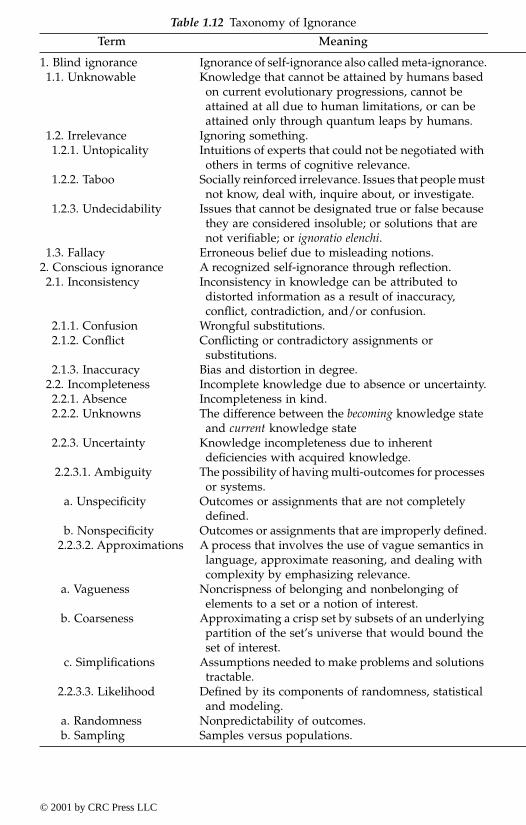
Table 1.12 Taxonomy of Ignorance
Term Meaning
1. Blind ignorance Ignorance of self-ignorance also called meta-ignorance. 1.1. Unknowable Knowledge that cannot be attained by humans based
on current evolutionary progressions, cannot be attained at all due to human limitations, or can be attained only through quantum leaps by humans.
1.2. Irrelevance Ignoring something. 1.2.1. Untopicality Intuitions of experts that could not be negotiated with
others in terms of cognitive relevance. 1.2.2. Taboo Socially reinforced irrelevance. Issues that people must
not know, deal with, inquire about, or investigate. 1.2.3. Undecidability Issues that cannot be designated true or false because
they are considered insoluble; or solutions that are not verifiable; or ignoratio elenchi.
1.3. Fallacy Erroneous belief due to misleading notions.2. Conscious ignorance A recognized self-ignorance through reflection. 2.1. Inconsistency Inconsistency in knowledge can be attributed to
distorted information as a result of inaccuracy, conflict, contradiction, and/or confusion.
2.1.1. Confusion Wrongful substitutions. 2.1.2. Conflict Conflicting or contradictory assignments or
substitutions. 2.1.3. Inaccuracy Bias and distortion in degree. 2.2. Incompleteness Incomplete knowledge due to absence or uncertainty. 2.2.1. Absence Incompleteness in kind. 2.2.2. Unknowns The difference between the becoming knowledge state
and current knowledge state 2.2.3. Uncertainty Knowledge incompleteness due to inherent
deficiencies with acquired knowledge. 2.2.3.1. Ambiguity The possibility of having multi-outcomes for processes
or systems. a. Unspecificity Outcomes or assignments that are not completely
defined. b. Nonspecificity Outcomes or assignments that are improperly defined. 2.2.3.2. Approximations A process that involves the use of vague semantics in
language, approximate reasoning, and dealing with complexity by emphasizing relevance.
a. Vagueness Noncrispness of belonging and nonbelonging of elements to a set or a notion of interest.
b. Coarseness Approximating a crisp set by subsets of an underlying partition of the set’s universe that would bound the set of interest.
c. Simplifications Assumptions needed to make problems and solutions tractable.
2.2.3.3. Likelihood Defined by its components of randomness, statistical and modeling.
a. Randomness Nonpredictability of outcomes. b. Sampling Samples versus populations.
© 2001 by CRC Press LLC
be attributed to intuitions of experts that could not be negotiated with othersin terms of cognitive relevance. Taboo is due to socially reinforced irrele-vance. Issues that people must not know, deal with, inquire about, or inves-tigate define the domain of taboo. The undecidability type deals with issuesthat cannot be designated true or false because they are considered insoluble,or solutions that are not verifiable, or as a result of ignoratio elenchi. A thirdcomponent of blind ignorance is fallacy that can be defined as erroneousbeliefs due to misleading notions.
Kurt Gödel (1906–1978) showed that a logical system could not be bothconsistent and complete and could not prove itself complete without provingitself inconsistent and vise versa. Also, he showed that there are problemsthat cannot be solved by any set of rules or procedures; instead, for theseproblems one must always extend the set of axioms. This philosophical viewof logic can be used as a basis for classifying the conscious ignorance intoinconsistency and incompleteness.
Inconsistency in knowledge can be attributed to distorted informationas a result of inaccuracy, conflict, contradiction, and/or confusion, as shownin Figure 1.9. Inconsistency can result from assignments and substitutionsthat are wrong, conflicting, or biased, producing confusion, conflict, or inac-curacy, respectively. The confusion and conflict result from in-kind inconsis-tent assignments and substitutions, whereas inaccuracy results from a levelbias or error in these assignments and substitutions.
Incompleteness is defined as incomplete knowledge and can be consid-ered to consist of (1) absence and unknowns as incompleteness in kind and(2) uncertainty. The unknowns or unknown knowledge can be viewed inevolutionary epistemology as the difference between the becoming knowl-edge state and current knowledge state. The knowledge absence componentcan lead to one of these scenarios: (1) no action and working without theknowledge, (2) unintentionally acquiring irrelevant knowledge, leading toblind ignorance, (3) acquiring relevant knowledge that can be with variousuncertainties and levels, or (4) deliberately acquiring irrelevant knowledge.The fourth possible scenario is frequently not listed, since it is not realistic.
Uncertainty can be defined as knowledge incompleteness due to inher-ent deficiencies with acquired knowledge. Uncertainty can be classified intothree types based on its sources: ambiguity, approximations, and likelihood.Ambiguity comes from the possibility of having multiple outcomes for pro-cesses or systems. Recognition of some of the possible outcomes createsuncertainty. The recognized outcomes might constitute only a partial list ofall possible outcomes leading to unspecificity. In this context, unspecificityresults from outcomes or assignments that are not completely defined. Theincorrect definition of outcomes, i.e., error in defining outcomes, can be callednonspecificity. In this context, nonspecificity results from outcomes or assign-ments that are improperly defined. Nonspecificity is a form of knowledgeabsence and can be treated similarly to the absence category under incom-pleteness. Nonspecificity can be viewed as a state of blind ignorance.
© 2001 by CRC Press LLC
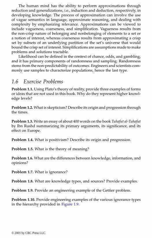
The human mind has the ability to perform approximations throughreduction and generalizations, i.e., induction and deduction, respectively, indeveloping knowledge. The process of approximation can involve the useof vague semantics in language, approximate reasoning, and dealing withcomplexity by emphasizing relevance. Approximations can be viewed toinclude vagueness, coarseness, and simplification. Vagueness results fromthe non-crisp nature of belonging and nonbelonging of elements to a set ora notion of interest, whereas coarseness results from approximating a crispset by subsets of an underlying partition of the set’s universe that wouldbound the crisp set of interest. Simplifications are assumptions made to makeproblems and solutions tractable.
Likelihood can be defined in the context of chance, odds, and gambling,and it has primary components of randomness and sampling. Randomnessstems from the non-predictability of outcomes. Engineers and scientists com-monly use samples to characterize populations, hence the last type.
1.6 Exercise ProblemsProblem 1.1. Using Plato’s theory of reality, provide three examples of formsor ideas that are not used in this book. Why do they represent higher knowl-edge levels?
Problem 1.2. What is skepticism? Describe its origin and progression throughthe times.
Problem 1.3. Write an essay of about 400 words on the book Tuhafut al-Tuhafutby Ibn Rushd summarizing its primary arguments, its significance, and itseffect on Europe.
Problem 1.4. What is positivism? Describe its origin and progression.
Problem 1.5. What is the theory of meaning?
Problem 1.6. What are the differences between knowledge, information, andopinions?
Problem 1.7. What is ignorance?
Problem 1.8. What are knowledge types, and sources? Provide examples.
Problem 1.9. Provide an engineering example of the Gettier problem.
Problem 1.10. Provide engineering examples of the various ignorance typesin the hierarchy provided in Figure 1.9.
© 2001 by CRC Press LLC

Problem 1.11. Provide an example from the sciences of the Gettier problem.
Problem 1.12. Provide examples from the sciences of the various ignorancetypes in the hierarchy provided in Figure 1.9.
Problem 1.13. What are the differences between an unknown and anunknowable? Provide examples.
© 2001 by CRC Press LLC

chapter two
Information-based system definition
Contents
2.1. Introduction2.2. System definition models
2.2.1. Perspectives for system definition2.2.2. Requirements and work breakdown structure
2.2.2.1. Requirements analysis2.2.2.2. Work breakdown structure
2.2.3. Process modeling method2.2.3.1. System engineering process2.2.3.2. Lifecycle of engineering systems2.2.3.3. Technical maturity model
2.2.4. Black-box method2.2.5. State-based method2.2.6. Component integration method2.2.7. Decision analysis method
2.2.7.1. Decision variables2.2.7.2. Decision outcomes2.2.7.3. Associated probabilities and consequences2.2.7.4. Decision trees2.2.7.5. Influence diagrams
2.3. Hierarchical definitions of systems2.3.1. Introduction2.3.2. Knowledge and information hierarchy
2.3.2.1. Source systems2.3.2.2. Data systems2.3.2.3. Generative systems2.3.2.4. Structure systems2.3.2.5. Metasystems
© 2001 by CRC Press LLC

2.4. Models for ignorance and uncertainty types2.4.1. Mathematical theories for ignorance types2.4.2. Information uncertainty in engineering systems
2.4.2.1. Abstraction and modeling of engineeringsystems
2.4.2.2. Ignorance and uncertainty in abstracted aspectsof a system
2.4.2.3. Ignorance and uncertainty in nonabstractedaspects of a system
2.4.2.4. Ignorance due to unknown aspects of a system2.5. System complexity2.6. Exercise problems
2.1 IntroductionThe definition and articulation of problems in engineering and science arecritical tasks in the processes of analysis and design and can be systemati-cally performed within a systems framework. “The mere formulation of aproblem is often far more essential than its solution,” Albert Einstein(1879–1955) said. “What we observe is not nature itself, but nature exposedto our method of questioning,” Werner Karl Heisenberg (1901–1976) said.Generally, a manmade or natural system, such as an engineering project,can be modeled to include a segment of its environment that interactssignificantly with it to define an underlying system. The boundaries of thesystem are drawn based on the goals and characteristics of the analysis, theclass of performances (including failures) under consideration, and theobjectives of the analysis.
A generalized systems formulation allows scientists and engineers todevelop a complete and comprehensive understanding of the nature of aproblem, underlying physics, processes, and activities. In a system formu-lation, an image or a model of an object that emphasizes some importantand critical properties is defined. System definition is usually the first stepin an overall methodology formulated for achieving a set of objectives. Thisdefinition can be based on observations at different system levels that areestablished based on these objectives. The observations can be about thedifferent elements (or components) of the system, interactions among theseelements, and the expected behavior of the system. Each level of knowledgethat is obtained about an engineering problem defines a system to representthe project or the problem. As additional levels of knowledge are added toprevious ones, higher epistemological levels of system definition anddescription are attained which, taken together, form a hierarchy of the systemdescriptions.
Informally, what is a system? According to the Webster’s dictionary, asystem is defined as “a regularly interacting or interdependent group ofitems forming a unified whole.” For scientists and engineers, the definitioncan be stated as “a regularly interacting or interdependent group of items
© 2001 by CRC Press LLC
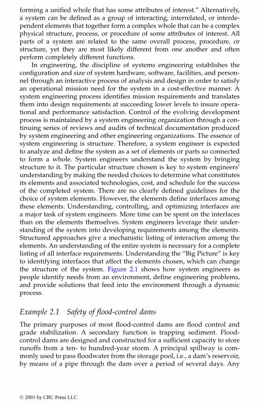
forming a unified whole that has some attributes of interest.” Alternatively,a system can be defined as a group of interacting, interrelated, or interde-pendent elements that together form a complex whole that can be a complexphysical structure, process, or procedure of some attributes of interest. Allparts of a system are related to the same overall process, procedure, orstructure, yet they are most likely different from one another and oftenperform completely different functions.
In engineering, the discipline of systems engineering establishes theconfiguration and size of system hardware, software, facilities, and person-nel through an interactive process of analysis and design in order to satisfyan operational mission need for the system in a cost-effective manner. Asystem engineering process identifies mission requirements and translatesthem into design requirements at succeeding lower levels to insure opera-tional and performance satisfaction. Control of the evolving developmentprocess is maintained by a system engineering organization through a con-tinuing series of reviews and audits of technical documentation producedby system engineering and other engineering organizations. The essence ofsystem engineering is structure. Therefore, a system engineer is expectedto analyze and define the system as a set of elements or parts so connectedto form a whole. System engineers understand the system by bringingstructure to it. The particular structure chosen is key to system engineers’understanding by making the needed choices to determine what constitutesits elements and associated technologies, cost, and schedule for the successof the completed system. There are no clearly defined guidelines for thechoice of system elements. However, the elements define interfaces amongthese elements. Understanding, controlling, and optimizing interfaces area major task of system engineers. More time can be spent on the interfacesthan on the elements themselves. System engineers leverage their under-standing of the system into developing requirements among the elements.Structured approaches give a mechanistic listing of interaction among theelements. An understanding of the entire system is necessary for a completelisting of all interface requirements. Understanding the “Big Picture” is keyto identifying interfaces that affect the elements chosen, which can changethe structure of the system. Figure 2.1 shows how system engineers aspeople identify needs from an environment, define engineering problems,and provide solutions that feed into the environment through a dynamicprocess.
Example 2.1 Safety of flood-control dams
The primary purposes of most flood-control dams are flood control andgrade stabilization. A secondary function is trapping sediment. Flood-control dams are designed and constructed for a sufficient capacity to storerunoffs from a ten- to hundred-year storm. A principal spillway is com-monly used to pass floodwater from the storage pool, i.e., a dam’s reservoir,by means of a pipe through the dam over a period of several days. Any
© 2001 by CRC Press LLC
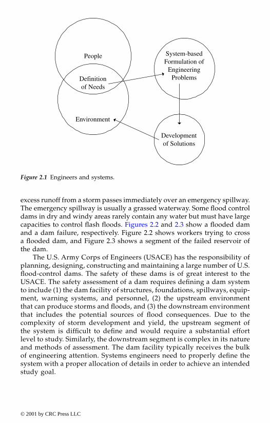
excess runoff from a storm passes immediately over an emergency spillway.The emergency spillway is usually a grassed waterway. Some flood controldams in dry and windy areas rarely contain any water but must have largecapacities to control flash floods. Figures 2.2 and 2.3 show a flooded damand a dam failure, respectively. Figure 2.2 shows workers trying to crossa flooded dam, and Figure 2.3 shows a segment of the failed reservoir ofthe dam.
The U.S. Army Corps of Engineers (USACE) has the responsibility ofplanning, designing, constructing and maintaining a large number of U.S.flood-control dams. The safety of these dams is of great interest to theUSACE. The safety assessment of a dam requires defining a dam systemto include (1) the dam facility of structures, foundations, spillways, equip-ment, warning systems, and personnel, (2) the upstream environmentthat can produce storms and floods, and (3) the downstream environmentthat includes the potential sources of flood consequences. Due to thecomplexity of storm development and yield, the upstream segment ofthe system is difficult to define and would require a substantial effortlevel to study. Similarly, the downstream segment is complex in its natureand methods of assessment. The dam facility typically receives the bulkof engineering attention. Systems engineers need to properly define thesystem with a proper allocation of details in order to achieve an intendedstudy goal.
Figure 2.1 Engineers and systems.
System-basedFormulation of
EngineeringProblems
People
Developmentof Solutions
Definitionof Needs
Environment
© 2001 by CRC Press LLC
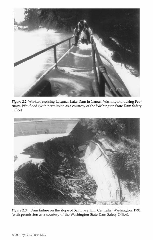
Figure 2.2 Workers crossing Lacamas Lake Dam in Camas, Washington, during Feb-ruary, 1996 flood (with permission as a courtesy of the Washington State Dam SafetyOffice).
Figure 2.3 Dam failure on the slope of Seminary Hill, Centralia, Washington, 1991 (with permission as a courtesy of the Washington State Dam Safety Office).
© 2001 by CRC Press LLC
2.2 System definition models 2.2.1 Perspectives for system definition
The term system originates from the Greek word systema that means anorganized whole. The Webster’s dictionary defines it as “a set or arrange-ment of things so related or connected as to form a unity or organic whole,”such as a solar system, school system, or system of highways. Also, it isdefined as “a set of facts, principles, rules, etc. classified or arranged in aregular, orderly form so as to show a logical plan linking the various parts.”The term system science is usually associated with observations, identification,description, experimental investigation, and theoretical modeling and expla-nations that are associated with natural phenomena in fields, such as biology,chemistry, and physics. System analysis includes ongoing analytical processesof evaluating various alternatives in design and model construction byemploying mathematical methods, for example, optimization, reliabilityassessment, statistics, risk analysis, and operations research.
Systems can be grouped in various categories, such as (1) naturalsystems, such as river systems, and energy systems; (2) manmade systemsthat can be imbedded in the natural systems, such as hydroelectric powersystems and navigation systems; (3) physical systems that are made ofreal components occupying space, such as automobiles and computers;(4) conceptual systems that could lead to physical systems; (5) static sys-tems that are without any activity, such as bridges subjected to dead loads;(6) dynamic systems, such as transportation systems; (7) closed or open-loop systems, such as a chemical equilibrium process and logistic systems,respectively. Blanchard (1998) provides additional information on thesecategories.
Systems analysis requires the development of models that need to berepresentative of system behavior by focusing on selected attributes of inter-est. Models for various categories, including natural or manmade systems,can be viewed as abstractions of their respective real systems. System scien-tists or engineers play a major role in defining the level of details of thisabstraction, and type and extent of information needed in order to properlyand adequately model these attributes and predict system behavior. In gen-eral, models can be viewed as assemblages of knowledge and informationon most relevant system behavior and attributes. The availability of knowl-edge and information, lack of them, and uncertainty play major roles indefining these models. This section summarizes various system models thatinclude (1) requirements analysis, (2) work breakdown structure, (3) processmodeling method, (4) black-box method, (5) state-based method, (6) compo-nent-integration method, and (7) decision-analysis method. It is very com-mon to use a combination of several models to represent a system in orderto achieve an analytical goal.
© 2001 by CRC Press LLC

2.2.2 Requirements and work breakdown structure
2.2.2.1 Requirements analysisThe definition of a system requires a goal that can be determined from eitherneed identification or a problem articulation. The goal statement should thenbe used to define a hierarchy of objectives that can be used to develop a listof performance and functional requirements for the system. Therefore, theserequirements form a basis for other system definition methods that aredescribed in subsequent sections.
A system model can be developed based on requirement and functionalmodeling. For example, dams can be modeled as systems with functionaland performance requirements in an environment that has natural and man-made hazards. By limiting the model only to the physical system of a dam,Figure 2.4 was developed for illustrative purposes. The functional require-ments of a dam are used to develop a system breakdown. The systembreakdown structure is the top down hierarchical division of the dam intoits subsystems and components, including people, structure, foundation,flood plain, river and its tributaries, procedures, and equipment. By dividingthe dam environment into major subsystems, an organized physical defini-tion for the dam system can be created. This definition allows for a betterevaluation of hazards and potential effects of these hazards. By evaluatingrisk hierarchically (top down) rather than in a fragmented manner, rational,repeatable, and systematic outcomes can be achieved.
Figure 2.4 Functional requirements for a dam.
Dam
ServiceabilityRequirements
Safety Requirements
WaterRelease
Pool WaterLevel
FloodControl
Strength
StabilityStructural/Geotechnical
IntegrityDownstream
DamsFlood Plain
© 2001 by CRC Press LLC
Requirements analysis can be defined as the detailed study of the sys-tem’s performance requirements to ensure that the completed systemachieves its intend utility to the customer and meets the goal stated. Accord-ing to this method, the customer’s needs should be determined, evaluatedfor their completeness, and translated into quantifiable, verifiable, and doc-umented performance requirements. Requirements analysis feeds directlyinto functional analysis, and allocation, design, and synthesis.
Functional analysis examines the characteristic actions of hardware, soft-ware, facilities, or personnel that are needed for the system in order to satisfyperformance requirements of the system. Functional analysis might establishadditional requirements on all supporting elements of the system by exam-ining their detailed operations and interactions. The overall set of systemrequirements derived by these analyses lead to both performance and func-tional requirements. Functional requirements define what the system mustdo and are characterized by verbs because they imply action on the part ofthe system. The system gathers, processes, transmits, informs, states, ini-tiates, and ceases. Also, physical requirements might be needed and can beincluded as a part of the performance requirements. Physical requirementsdefine the system’s physical nature, such as mass, volume, power, through-put, memory, and momentum. They may also include details down to typeand color of paint, location of the ground segment equipment, and specificenvironmental protection. For example, aerospace company systems, unlikemany commercial products, strongly emphasize the functional requirements,thus prompting the need for a significant evaluation of the system’s func-tional requirements and the allocation of those requirements to the physicalarchitecture.
The functional requirements can be loosely assembled into a hierarchyof functional, sequential, communication, procedural, temporal, or logicalmanner as follows:
• Functional requirements with subfunctions that contribute directlyto performing a single function;
• Sequential breakdowns that show data flow processed sequentiallyfrom input to output;
• Communication breakdowns based on information and data needs;• Procedural breakdowns based on logic flow paths;• Temporal breakdowns for differing functions at different times; and• Logical breakdowns based on developing logical flows for functions.
Many programs develop multiple functional hierarchies, using morethan one of these criteria to sort and decompose the functions. Each criterionprovides a different way of looking at the information, which is useful forsolving different types of problems. The most common functional hierarchyis a decomposition based on functional grouping, where the lower tier func-tions taken in total describe the activity of the upper tier function, providinga more detailed description of their top-level functions.
© 2001 by CRC Press LLC
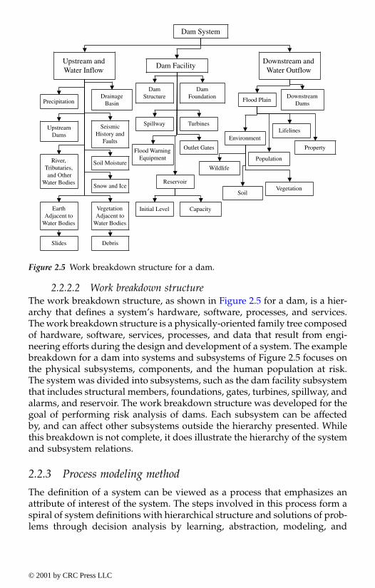
2.2.2.2 Work breakdown structureThe work breakdown structure, as shown in Figure 2.5 for a dam, is a hier-archy that defines a system’s hardware, software, processes, and services.The work breakdown structure is a physically-oriented family tree composedof hardware, software, services, processes, and data that result from engi-neering efforts during the design and development of a system. The examplebreakdown for a dam into systems and subsystems of Figure 2.5 focuses onthe physical subsystems, components, and the human population at risk.The system was divided into subsystems, such as the dam facility subsystemthat includes structural members, foundations, gates, turbines, spillway, andalarms, and reservoir. The work breakdown structure was developed for thegoal of performing risk analysis of dams. Each subsystem can be affectedby, and can affect other subsystems outside the hierarchy presented. Whilethis breakdown is not complete, it does illustrate the hierarchy of the systemand subsystem relations.
2.2.3 Process modeling method
The definition of a system can be viewed as a process that emphasizes anattribute of interest of the system. The steps involved in this process form aspiral of system definitions with hierarchical structure and solutions of prob-lems through decision analysis by learning, abstraction, modeling, and
Figure 2.5 Work breakdown structure for a dam.
Dam System
Dam FacilityDownstream andWater Outflow
DamFoundation
DamStructure Downstream
DamsFlood Plain
Property
Environment
Wildlife
Lifelines
Upstream andWater Inflow
DrainageBasinPrecipitation
Soil Moisture
Snow and Ice
River,Tributaries,and Other
Water Bodies
UpstreamDams
VegetationAdjacent to
Water Bodies
EarthAdjacent to
Water Bodies
Slides Debris
TurbinesSpillway
Outlet GatesFlood WarningEquipment
CapacityInitial Level
Reservoir
SeismicHistory and
Faults
VegetationSoil
Population
© 2001 by CRC Press LLC
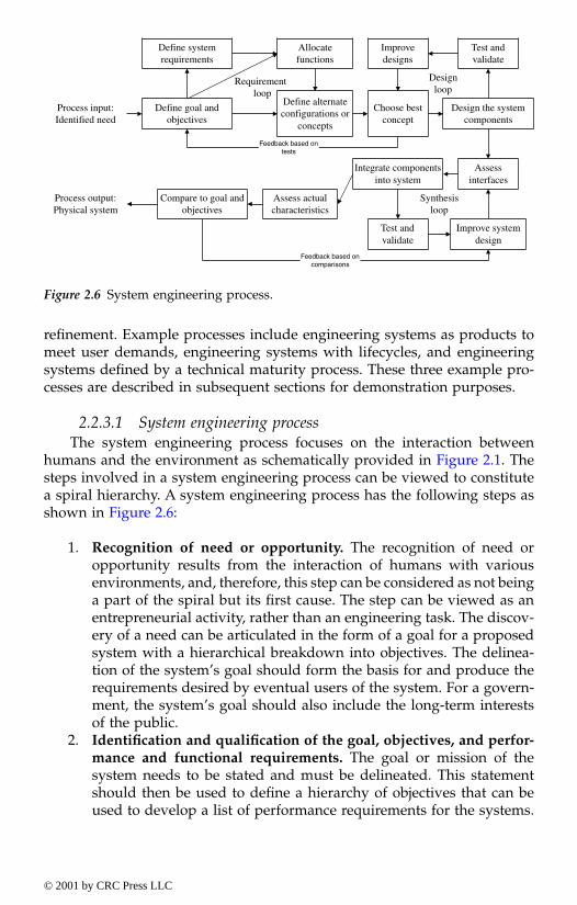
refinement. Example processes include engineering systems as products tomeet user demands, engineering systems with lifecycles, and engineeringsystems defined by a technical maturity process. These three example pro-cesses are described in subsequent sections for demonstration purposes.
2.2.3.1 System engineering processThe system engineering process focuses on the interaction between
humans and the environment as schematically provided in Figure 2.1. Thesteps involved in a system engineering process can be viewed to constitutea spiral hierarchy. A system engineering process has the following steps asshown in Figure 2.6:
1. Recognition of need or opportunity. The recognition of need oropportunity results from the interaction of humans with variousenvironments, and, therefore, this step can be considered as not beinga part of the spiral but its first cause. The step can be viewed as anentrepreneurial activity, rather than an engineering task. The discov-ery of a need can be articulated in the form of a goal for a proposedsystem with a hierarchical breakdown into objectives. The delinea-tion of the system’s goal should form the basis for and produce therequirements desired by eventual users of the system. For a govern-ment, the system’s goal should also include the long-term interestsof the public.
2. Identification and qualification of the goal, objectives, and perfor-mance and functional requirements. The goal or mission of thesystem needs to be stated and must be delineated. This statementshould then be used to define a hierarchy of objectives that can beused to develop a list of performance requirements for the systems.
Figure 2.6 System engineering process.
Process input:Identified need
Define goal andobjectives
Define systemrequirements
Allocatefunctions
Define alternateconfigurations or
concepts
Feedback based oncomparisons
Choose bestconcept
Design the systemcomponents
Test andvalidate
Improvedesigns
Designloop
Requirementloop
Test andvalidate
Improve systemdesign
Assessinterfaces
Integrate componentsinto system
Synthesisloop
Assess actualcharacteristics
Compare to goal andobjectives
Process output:Physical system
Feedback based ontests
© 2001 by CRC Press LLC
These definitions of the goal, objectives and performance require-ments can be used to compare the cost effectiveness of alternativesystem design concepts. The objectives and performance require-ments should include relevant aspects of effectiveness, cost, scheduleand risk, and they should be traceable to the goal. To facilitate tradeoffanalyses, they should be stated in quantifiable and verifiable termsto some meaningful extents. At each turn of a loop or spiral, theobjectives and performance requirements should be documented fortraceability to various system components. As the systems engineer-ing process continues, the performance requirements need to betranslated into a functional hierarchy for the system allocated to thesystem’s components. The performance and functional requirementsshould be quantitatively described.
3. Creation of alternative design concepts. Establishing a clear under-standing of what the system needs to accomplish is a prerequisite todevising a variety of ways that the goal, objectives, and requirementscan be met. Sometimes, the alternatives can come about as a conse-quence of integrating available component design options. Using abottom-up alternative creation, various concept designs can be de-veloped. It is essential to maintain objectivity to the process withoutbeing drawn to a specific option that would limit or obscure theexamination of other options. An analyst or designer must stay anoutsider in order to maintain objectivity. This detachment wouldallow the analyst or designer to avoid a premature focus on a singledesign and would permit discovery of a truly superior design.
4. Testing and validation. At this stage, some testing and validation ofthe concepts might be necessary in order to establish an understand-ing of the limitations, capabilities, and characteristics of various con-cepts. The testing and validation can be experimentally, analytically,or numerically performed using laboratory tests, analytical models,or simulation, respectively. The insight gained from this step mightbe crucial for subsequent steps of this process.
5. Performance of tradeoff studies and selection of a design. Tradeoffstudies start by assessing how well each design concept meets thesystem’s goal, objectives, and requirements including effectiveness,cost, schedule, and risk, both quantitatively and otherwise. This as-sessment can utilize the testing and validation results of the previousstep. These studies can be performed using system models that an-alytically relate various concept characteristics to performance andfunctional requirements. An outcome of these studies can be thedetermination of bounds on the relative cost effectiveness of thedesign concepts. Selection among the alternative design conceptsmust take into account subjective factors that are not quantifiable andwere not incorporated in the studies. When possible, mathematicalexpressions, called objective functions, should be developed andused to express the values of combinations of possible outcomes as
© 2001 by CRC Press LLC
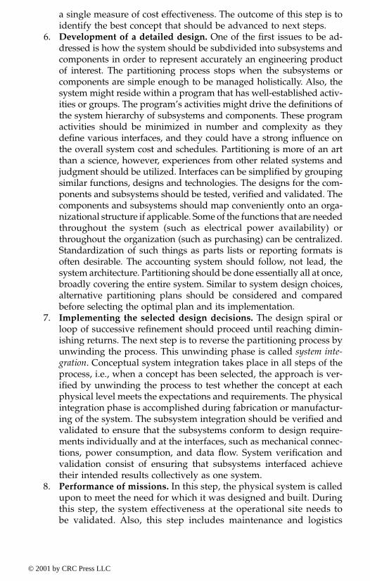
a single measure of cost effectiveness. The outcome of this step is toidentify the best concept that should be advanced to next steps.
6. Development of a detailed design. One of the first issues to be ad-dressed is how the system should be subdivided into subsystems andcomponents in order to represent accurately an engineering productof interest. The partitioning process stops when the subsystems orcomponents are simple enough to be managed holistically. Also, thesystem might reside within a program that has well-established activ-ities or groups. The program’s activities might drive the definitions ofthe system hierarchy of subsystems and components. These programactivities should be minimized in number and complexity as theydefine various interfaces, and they could have a strong influence onthe overall system cost and schedules. Partitioning is more of an artthan a science, however, experiences from other related systems andjudgment should be utilized. Interfaces can be simplified by groupingsimilar functions, designs and technologies. The designs for the com-ponents and subsystems should be tested, verified and validated. Thecomponents and subsystems should map conveniently onto an orga-nizational structure if applicable. Some of the functions that are neededthroughout the system (such as electrical power availability) orthroughout the organization (such as purchasing) can be centralized.Standardization of such things as parts lists or reporting formats isoften desirable. The accounting system should follow, not lead, thesystem architecture. Partitioning should be done essentially all at once,broadly covering the entire system. Similar to system design choices,alternative partitioning plans should be considered and comparedbefore selecting the optimal plan and its implementation.
7. Implementing the selected design decisions. The design spiral orloop of successive refinement should proceed until reaching dimin-ishing returns. The next step is to reverse the partitioning process byunwinding the process. This unwinding phase is called system inte-gration. Conceptual system integration takes place in all steps of theprocess, i.e., when a concept has been selected, the approach is ver-ified by unwinding the process to test whether the concept at eachphysical level meets the expectations and requirements. The physicalintegration phase is accomplished during fabrication or manufactur-ing of the system. The subsystem integration should be verified andvalidated to ensure that the subsystems conform to design require-ments individually and at the interfaces, such as mechanical connec-tions, power consumption, and data flow. System verification andvalidation consist of ensuring that subsystems interfaced achievetheir intended results collectively as one system.
8. Performance of missions. In this step, the physical system is calledupon to meet the need for which it was designed and built. Duringthis step, the system effectiveness at the operational site needs tobe validated. Also, this step includes maintenance and logistics
© 2001 by CRC Press LLC
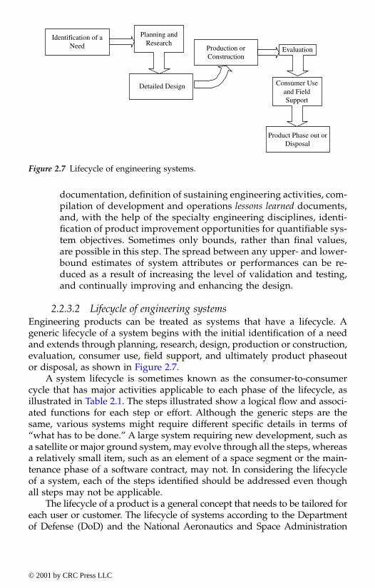
documentation, definition of sustaining engineering activities, com-pilation of development and operations lessons learned documents,and, with the help of the specialty engineering disciplines, identi-fication of product improvement opportunities for quantifiable sys-tem objectives. Sometimes only bounds, rather than final values,are possible in this step. The spread between any upper- and lower-bound estimates of system attributes or performances can be re-duced as a result of increasing the level of validation and testing,and continually improving and enhancing the design.
2.2.3.2 Lifecycle of engineering systemsEngineering products can be treated as systems that have a lifecycle. Ageneric lifecycle of a system begins with the initial identification of a needand extends through planning, research, design, production or construction,evaluation, consumer use, field support, and ultimately product phaseoutor disposal, as shown in Figure 2.7.
A system lifecycle is sometimes known as the consumer-to-consumercycle that has major activities applicable to each phase of the lifecycle, asillustrated in Table 2.1. The steps illustrated show a logical flow and associ-ated functions for each step or effort. Although the generic steps are thesame, various systems might require different specific details in terms of“what has to be done.” A large system requiring new development, such asa satellite or major ground system, may evolve through all the steps, whereasa relatively small item, such as an element of a space segment or the main-tenance phase of a software contract, may not. In considering the lifecycleof a system, each of the steps identified should be addressed even thoughall steps may not be applicable.
The lifecycle of a product is a general concept that needs to be tailored foreach user or customer. The lifecycle of systems according to the Departmentof Defense (DoD) and the National Aeronautics and Space Administration
Figure 2.7 Lifecycle of engineering systems.
Identification of aNeed
Planning andResearch
Evaluation
Detailed Design
Production orConstruction
Product Phase out orDisposal
Consumer Useand FieldSupport
© 2001 by CRC Press LLC
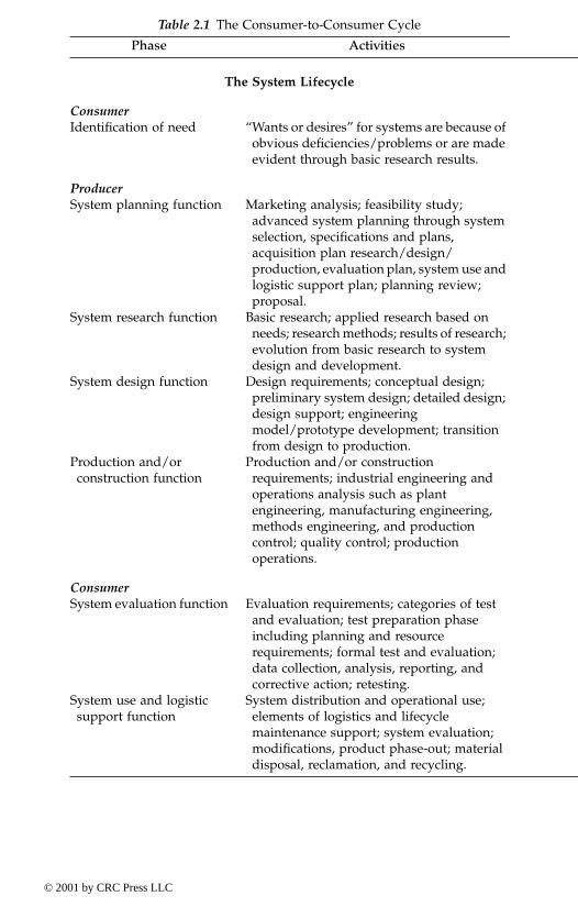
Table 2.1 The Consumer-to-Consumer Cycle
Phase Activities
The System Lifecycle
ConsumerIdentification of need “Wants or desires” for systems are because of
obvious deficiencies/problems or are made evident through basic research results.
ProducerSystem planning function Marketing analysis; feasibility study;
advanced system planning through system selection, specifications and plans, acquisition plan research/design/ production, evaluation plan, system use and logistic support plan; planning review; proposal.
System research function Basic research; applied research based on needs; research methods; results of research; evolution from basic research to system design and development.
System design function Design requirements; conceptual design; preliminary system design; detailed design; design support; engineering model/prototype development; transition from design to production.
Production and/or construction function
Production and/or construction requirements; industrial engineering and operations analysis such as plant engineering, manufacturing engineering, methods engineering, and production control; quality control; production operations.
ConsumerSystem evaluation function Evaluation requirements; categories of test
and evaluation; test preparation phase including planning and resource requirements; formal test and evaluation; data collection, analysis, reporting, and corrective action; retesting.
System use and logistic support function
System distribution and operational use; elements of logistics and lifecycle maintenance support; system evaluation; modifications, product phase-out; material disposal, reclamation, and recycling.
© 2001 by CRC Press LLC

(NASA) are tied to the government procurement process, as discussed in theNASA Example 2.1, but the general applicability of the concept of a systemlifecycle is independent of the user and the procurement process.
Example 2.1 Lifecycle of NASA engineering systems
The National Aeronautics and Space Administration (NASA) uses the con-cept of lifecycle for a program, called a program lifecycle which consists ofdistinct phases separated by control gates. NASA uses its lifecycle model notonly to describe how a program evolves over time, but also to aid manage-ment in program control. The boundaries between phases are defined so thatthey provide proceed or do not proceed decisions. Decisions to proceed may bequalified by liens that must be removed within a reasonable time. A programthat fails to pass a control gate and has enough resources may be allowed toreaddress the deficiencies or it may be terminated.
The government operates with a fiscal budget and annual funding lead-ing to implicit funding control gates at the beginning of each fiscal year.While these gates place planning requirements on the project and can makesignificant replanning necessary, they are not part of an orderly systemengineering process; rather, they constitute one of the sources of uncertaintythat affect project risks and should be included in project risk considerations.
The NASA model can generally be defined to include the followingphases:
Prephase A — Advanced StudiesThe objective of this phase is to produce a broad spectrum of ideas and
alternatives for missions from which new projects or programs can beselected. Major activities and their products in this prephase A are to(1) identify missions consistent with the NASA charter, (2) identify andinvolve users, and (3) perform preliminary evaluations of possible missions.Typically, this phase consists of loosely structured examinations of new ideas,usually without central control and mostly oriented toward small studies.Also, program or project proposals are prepared that include mission justifi-cation and objectives, possible operations concepts, possible system architec-tures, and cost, schedule, and risk estimates. The phase also produces masterplans for existing program areas. The control gate for this phase is informalproposal reviews. Descriptions of projects suggested generally include initialsystem design and operational concepts, preliminary project organization,schedule, testing and review structure, and documentation requirements.
This phase is of an ongoing nature since technological progress makespossible missions that were previously impossible. Manned trips to the moonand the taking of high-resolution pictures of planets and other objects in theuniverse illustrate past responses to this kind of opportunity. New opportu-nities will continue to become available as our technological capabilities grow.
© 2001 by CRC Press LLC

Phase A — Conceptual design studiesThe objective of this phase is to determine the feasibility and desirability
of a suggested new major system in preparation for the seeking of funding.This phase includes major activities such as (1) preparation of mission needsstatements, (2) development of preliminary system requirements, (3) identi-fication of alternative operations and logistics concepts, (4) identification ofproject constraints and system boundaries, (5) consideration of alternativedesign concepts, and (6) demonstrating that credible, feasible designs exist.System validation plans are initiated in this phase. Also, systems engineeringtools and models are acquired, environmental impact studies are initiated,and program implementation plans are prepared. The control gates are con-ceptual design review and prephase B nonadvocate review. This phase isfrequently described as a structured version of the previous phase.
Phase B — Concept definitionThe objective of this phase is to define the project in enough detail to
establish an initial baseline. This phase includes major activities such as
• reaffirmation of the mission needs statement,• preparation of a program initiation agreement,• preparation of a system engineering management plan,• preparation of a risk management plan,• initiation of configuration management,• development of a system-level cost-effectiveness model,• restatement of the mission needs as system requirements,• establishment of the initial requirements traceability matrix,• selection of a baseline system architecture at some level of resolution
and concept of operation,• identification of science payload,• definition of internal and external interface requirements,• definition of the work breakdown structure,• definition of verification approach and policies, • preparation of preliminary manufacturing plans,• identification of government resource requirements,• identification of ground test and facility requirements,• development of statement of work,• revision and publication of project implementation plans,• initiation of advanced technology development programs.
The control gates include project definition and cost review, programand project requirements review, and safety review.
Tradeoff studies in this phase should precede rather than follow systemdesign decisions. A feasible system design can be defined as a design thatcan be implemented as designed, and can then accomplish the system’s goalwithin the constraints imposed by the fiscal and operating environment. Tobe credible, a design must not depend on the occurrence of unforeseen
© 2001 by CRC Press LLC

breakthroughs in the state of the art. While a credible design may assumelikely improvements in the state of the art, it is nonetheless riskier than onethat does not.
Phase C — Design and developmentThis phase has the objective to design a system and its associated sub-
systems, including its operations systems, so that it will be able to meet itsrequirements. This phase has primary tasks and activities that include
• adding subsystem design specifications to the system architecture,• publishing subsystem requirements documents,• preparation of subsystem verification plans,• preparation of interface documents,• repetition of the process of successive refinement to get “design-to”
and “build-to” specifications and drawings, verification plans, andinterface documents at all levels,
• augmentation of documents to reflect the growing maturity of thesystem,
• monitoring the project progress against project plans, • development of the system integration plan and the system opera-
tions plans,• documentation of tradeoff studies performed,• development of the end-to-end information system design and the
system deployment approach,• identification of opportunities for preplanned product improvement,
and• confirmation of science payload selection.
Control gates include system-level preliminary design review, sub-system (and lower level) preliminary design reviews, subsystem (and lowerlevel) critical design reviews, and system-level critical design review.
The purpose of this phase is to unfold system requirements into systemand subsystem designs. Several popular approaches can be used in theunfolding process, such as the code-and-fix, the waterfall, requirements-driven design, and/or evolutionary development.
Phase D — Fabrication, integration, test and certificationThe purpose of this phase is to build the system designed in the previous
phase. Activities include fabrication system of hardware and coding of soft-ware, integration, verification and validation, and certified acceptance of thesystem.
Phase E — Pre-operationsThe purpose of this phase is to prepare the certified system for operations
by performing main activities that include the initial training of operatingpersonnel and finalization of the integrated logistics support plan. For flightprojects, the focus of activities then shifts to prelaunch integration and
© 2001 by CRC Press LLC

launch. On the other hand, for large flight projects, extended periods of orbitinsertion, assembly, and shakedown operations are needed. In some projects,these activities can be treated as minor items permitting combining thisphase with either its predecessor or its successor. The control gates are launchreadiness reviews, operational readiness reviews, and safety reviews.
Phase F — Operations and disposalThe objective of this phase is to actually meet the initially identified
need, and then to dispose of the system in a responsible manner. This phaseincludes major activities such as (1) training replacement operators, (2) con-ducting the mission, (3) maintaining the operating system, and (4) disposingof the system. The control gates are operational acceptance review, regularsystem operations reviews, and system upgrade reviews.
Phase F encompasses the problem of dealing with the system when ithas completed its mission. The end of life depends on many factors. Forexample, the disposal of a flight system with short-mission duration, suchas a space-lab payload, may require only selection and retrieval of the hard-ware and its return to its owner, whereas a large flight project of longduration disposal may proceed according to long-established plans or maybegin as a result of unplanned events, such as accidents. In addition touncertainty as to when this part of the phase begins, the activities associatedwith safely deactivating and disposing of a system may be long and complex.As a result, the costs and risks associated with different designs should beconsidered during the planning process.
2.2.3.3 Technical maturity modelThe technical maturity model is another view of the lifecycle of a project.According to this model, the lifecycle considers a program as an interactionbetween society and engineering. The model concentrates on the engineeringaspects of the program and not on the technology development throughresearch. The program must come to fruition by meeting both the needs ofthe customer and also meeting the technical requirements. Therefore, bykeeping distinctions among technical requirements, needs and technologydevelopment, the motivations, wants, and desires of the customer are dif-ferentiated from the technology issues during the course of the project.
2.2.4 Black-box method
Historically, engineers have built analytical models to represent natural andmanmade systems using empirical tools of observing system attributes ofinterest (called system output variables) and trying to relate them to someother controllable or uncontrollable input variables. For example, a structuralengineer might observe the deflection of a bridge as an output of an inputsuch as a load at middle of its span. By varying the intensity of the load, thedeflection changes. Empirical test methods would vary the load incremen-tally and the corresponding deflections are measured, thereby producing arelationship such as
© 2001 by CRC Press LLC
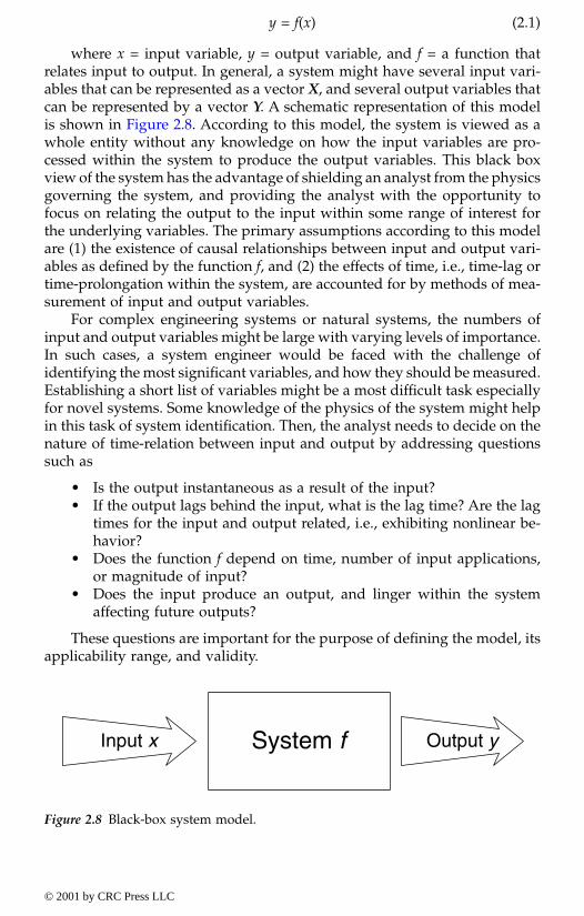
y = f(x) (2.1)
where x = input variable, y = output variable, and f = a function thatrelates input to output. In general, a system might have several input vari-ables that can be represented as a vector X, and several output variables thatcan be represented by a vector Y. A schematic representation of this modelis shown in Figure 2.8. According to this model, the system is viewed as awhole entity without any knowledge on how the input variables are pro-cessed within the system to produce the output variables. This black boxview of the system has the advantage of shielding an analyst from the physicsgoverning the system, and providing the analyst with the opportunity tofocus on relating the output to the input within some range of interest forthe underlying variables. The primary assumptions according to this modelare (1) the existence of causal relationships between input and output vari-ables as defined by the function f, and (2) the effects of time, i.e., time-lag ortime-prolongation within the system, are accounted for by methods of mea-surement of input and output variables.
For complex engineering systems or natural systems, the numbers ofinput and output variables might be large with varying levels of importance.In such cases, a system engineer would be faced with the challenge ofidentifying the most significant variables, and how they should be measured.Establishing a short list of variables might be a most difficult task especiallyfor novel systems. Some knowledge of the physics of the system might helpin this task of system identification. Then, the analyst needs to decide on thenature of time-relation between input and output by addressing questionssuch as
• Is the output instantaneous as a result of the input?• If the output lags behind the input, what is the lag time? Are the lag
times for the input and output related, i.e., exhibiting nonlinear be-havior?
• Does the function f depend on time, number of input applications,or magnitude of input?
• Does the input produce an output, and linger within the systemaffecting future outputs?
These questions are important for the purpose of defining the model, itsapplicability range, and validity.
Figure 2.8 Black-box system model.
System fInput x Output y
© 2001 by CRC Press LLC

Example 2.2 Probable maximum flood
The U.S. Army Corps of Engineers (USACE) classes dams according to bothsize and hazard, where hazard is defined in terms of potential loss of lifeand economic loss (Committee on Safety Criteria for Dams, 1985). Smalldams are 25 to 40 ft high, intermediate dams are 40 to 100 ft high, and largedams are over 100 ft high. Low hazard dams are those for which failure ofthe dam would result in no loss of life and only minimal economic loss. Asignificant hazard is one that would cause a few losses of life and appreciableeconomic loss, and a high hazard would result in the loss of more than afew lives and excessive economic loss.
The USACE uses three methods of determining extreme floods, depend-ing on the return period and intended use (USACE, 1965). Frequency anal-yses are used when the project demands a storm event with a relativelycommon return period and are based on gage records. This type of analysisis used for low hazard dams, small to intermediate dams in size, or smalldams with significant hazard classifications. A standard project flood (SPF)is used when some risk can be tolerated but where an unusually high degreeof protection is justified because of risk to life and property (Ponce, 1989).The SPF includes severe combinations of meteorological and hydrologicalconditions but does not include extremely rare combinations. The SPF istypically used for dams that are classed as a significant hazard and interme-diate to large in size. For projects requiring substantial reduction in risk,such as dams classed as a high hazard, the probable maximum flood (PMF)is used. The PMF is caused by the most severe and extreme combination ofmeteorological and hydrological events that could possibly occur in an area.Flood prediction can be based on black-box models as shown in Figure 2.9.For river systems, time can play a major role in the form of time lag, timeprolongation, and system nonlinearity.
Frequency analyses of gaged data conducted by the USACE are basedon recommendations in Bulletin 17B (U.S. Interagency Advisory Committeeon Water Data, 1982). The SPF is developed from a standard project storm.The PMF is based on an index rainfall and a depth-area-duration relation-ship. A hydrograph is then developed based on this rainfall minus hydro-logic extractions. For basins less than 1000 mi2 (2590 km2), the storms areusually based on localized thunderstorms; for basins greater than 1000 mi2
(2590 km2), the storms are usually a combination of events. Due to thesedifferences, the PMF for the smaller basins is based on a 6-hr or 12-hr timeincrement. For large basins, this procedure is considerably more complex.The SPF is developed very similarly to the PMF except that the index floodis decreased by about 50%.
The use of the PMF has often been questioned since rainfalls and floodsof that magnitude have not been experienced in a lifetime. However, studiesconducted by the USACE have shown that dozens of storms across the U.S.have exceeded 1/2 of the probable maximum precipitation (PMP) for thatarea (USACE, 1982; Committee on the Safety of Existing Dams, 1983). Based
© 2001 by CRC Press LLC
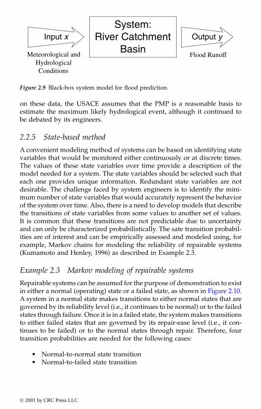
on these data, the USACE assumes that the PMP is a reasonable basis toestimate the maximum likely hydrological event, although it continued tobe debated by its engineers.
2.2.5 State-based method
A convenient modeling method of systems can be based on identifying statevariables that would be monitored either continuously or at discrete times.The values of these state variables over time provide a description of themodel needed for a system. The state variables should be selected such thateach one provides unique information. Redundant state variables are notdesirable. The challenge faced by system engineers is to identify the mini-mum number of state variables that would accurately represent the behaviorof the system over time. Also, there is a need to develop models that describethe transitions of state variables from some values to another set of values.It is common that these transitions are not predictable due to uncertaintyand can only be characterized probabilistically. The sate transition probabil-ities are of interest and can be empirically assessed and modeled using, forexample, Markov chains for modeling the reliability of repairable systems(Kumamoto and Henley, 1996) as described in Example 2.3.
Example 2.3 Markov modeling of repairable systems
Repairable systems can be assumed for the purpose of demonstration to existin either a normal (operating) state or a failed state, as shown in Figure 2.10.A system in a normal state makes transitions to either normal states that aregoverned by its reliability level (i.e., it continues to be normal) or to the failedstates through failure. Once it is in a failed state, the system makes transitionsto either failed states that are governed by its repair-ease level (i.e., it con-tinues to be failed) or to the normal states through repair. Therefore, fourtransition probabilities are needed for the following cases:
• Normal-to-normal state transition• Normal-to-failed state transition
Figure 2.9 Black-box system model for flood prediction.
System:River Catchment
BasinInput x Output y
Meteorological andHydrologicalConditions
Flood Runoff
© 2001 by CRC Press LLC
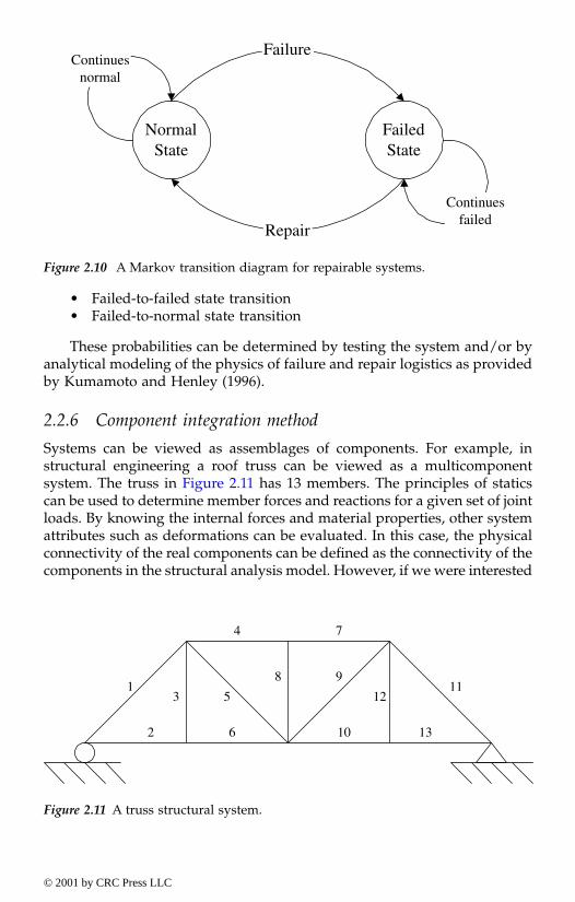
• Failed-to-failed state transition• Failed-to-normal state transition
These probabilities can be determined by testing the system and/or byanalytical modeling of the physics of failure and repair logistics as providedby Kumamoto and Henley (1996).
2.2.6 Component integration method
Systems can be viewed as assemblages of components. For example, instructural engineering a roof truss can be viewed as a multicomponentsystem. The truss in Figure 2.11 has 13 members. The principles of staticscan be used to determine member forces and reactions for a given set of jointloads. By knowing the internal forces and material properties, other systemattributes such as deformations can be evaluated. In this case, the physicalconnectivity of the real components can be defined as the connectivity of thecomponents in the structural analysis model. However, if we were interested
Figure 2.10 A Markov transition diagram for repairable systems.
Figure 2.11 A truss structural system.
NormalState
FailedState
Failure
Repair
Continuesnormal
Continuesfailed
1
2
3
4
5
6
7
8 9
10
1112
13
© 2001 by CRC Press LLC
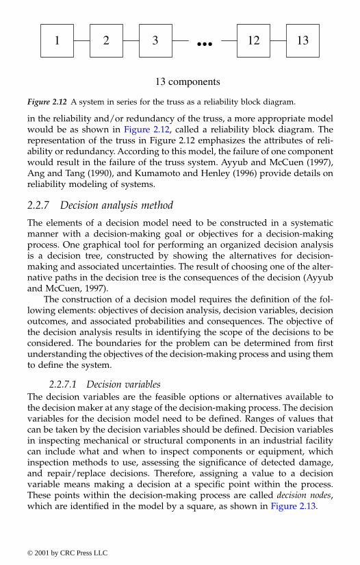
in the reliability and/or redundancy of the truss, a more appropriate modelwould be as shown in Figure 2.12, called a reliability block diagram. Therepresentation of the truss in Figure 2.12 emphasizes the attributes of reli-ability or redundancy. According to this model, the failure of one componentwould result in the failure of the truss system. Ayyub and McCuen (1997),Ang and Tang (1990), and Kumamoto and Henley (1996) provide details onreliability modeling of systems.
2.2.7 Decision analysis method
The elements of a decision model need to be constructed in a systematicmanner with a decision-making goal or objectives for a decision-makingprocess. One graphical tool for performing an organized decision analysisis a decision tree, constructed by showing the alternatives for decision-making and associated uncertainties. The result of choosing one of the alter-native paths in the decision tree is the consequences of the decision (Ayyuband McCuen, 1997).
The construction of a decision model requires the definition of the fol-lowing elements: objectives of decision analysis, decision variables, decisionoutcomes, and associated probabilities and consequences. The objective ofthe decision analysis results in identifying the scope of the decisions to beconsidered. The boundaries for the problem can be determined from firstunderstanding the objectives of the decision-making process and using themto define the system.
2.2.7.1 Decision variablesThe decision variables are the feasible options or alternatives available tothe decision maker at any stage of the decision-making process. The decisionvariables for the decision model need to be defined. Ranges of values thatcan be taken by the decision variables should be defined. Decision variablesin inspecting mechanical or structural components in an industrial facilitycan include what and when to inspect components or equipment, whichinspection methods to use, assessing the significance of detected damage,and repair/replace decisions. Therefore, assigning a value to a decisionvariable means making a decision at a specific point within the process.These points within the decision-making process are called decision nodes,which are identified in the model by a square, as shown in Figure 2.13.
Figure 2.12 A system in series for the truss as a reliability block diagram.
1 1332 ... 12
13 components
© 2001 by CRC Press LLC
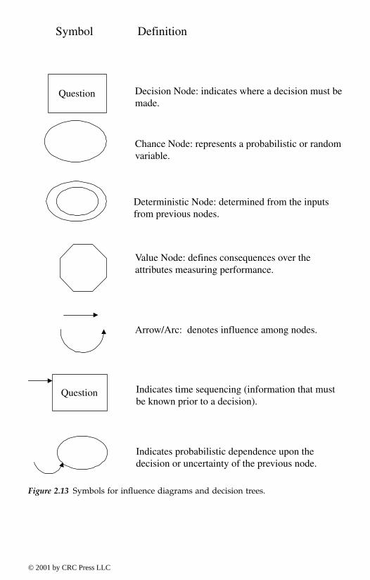
Figure 2.13 Symbols for influence diagrams and decision trees.
Question
Symbol
Decision Node: indicates where a decision must bemade.
Definition
Question
Chance Node: represents a probabilistic or randomvariable.
Deterministic Node: determined from the inputsfrom previous nodes.
Value Node: defines consequences over theattributes measuring performance.
Arrow/Arc: denotes influence among nodes.
Indicates time sequencing (information that mustbe known prior to a decision).
Indicates probabilistic dependence upon thedecision or uncertainty of the previous node.
© 2001 by CRC Press LLC

2.2.7.2 Decision outcomesThe decision outcomes for the decision model need also to be defined. Thedecision outcomes are the events that can happen as a result of a decision.They are random in nature, and their occurrence cannot be fully controlledby the decision maker. Decision outcomes can include the outcomes of aninspection (detection or nondetection of a damage) and the outcomes of arepair (satisfactory or nonsatisfactory repair). Therefore, the decision out-comes with the associated occurrence probabilities need to be defined. Thedecision outcomes can occur after making a decision at points within thedecision-making process called chance nodes, which are identified in themodel using a circle, as shown in Figure 2.13.
2.2.7.3 Associated probabilities and consequencesThe decision outcomes take values that can have associated probabilitiesand consequences. The probabilities are needed due to the random (chance)nature of these outcomes. The consequences can include, for example, thecost of failure due to damage that was not detected by an inspectionmethod.
2.2.7.4 Decision treesDecision trees are commonly used to examine the available information forthe purpose of decision making. The decision tree includes the decision andchance nodes. The decision nodes, that are represented by squares in adecision tree, are followed by possible actions (or alternatives, Ai) that canbe selected by a decision maker. The chance nodes, that are represented bycircles in a decision tree, are followed by outcomes that can occur withoutthe complete control of the decision maker. The outcomes have both prob-abilities (P) and consequences (C). Here the consequence can be cost. Eachtree segment followed from the beginning (left end) of the tree to the end(right end) of the tree is called a branch. Each branch represents a possiblescenario of decisions and possible outcomes. The total expected consequence(cost) for each branch could be computed. Then the most suitable decisionscan be selected to obtain the minimum cost. In general, utility values can beused and maximized instead of cost values. Also, decisions can be based onrisk profiles by considering both the total expected utility value and thestandard deviation of the utility value for each alternative. The standarddeviation can be critical for decision-making as it provides a measure ofuncertainty in utility values of alternatives (Kumamoto and Henley, 1996).Influence diagrams can be constructed to model dependencies among deci-sion variables, outcomes, and system states using the same symbols of Figure2.13. In the case of influence diagrams, arrows are used to represent depen-dencies between linked items, as described in Section 2.2.7.5.
© 2001 by CRC Press LLC
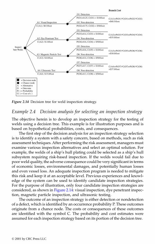
Example 2.4 Decision analysis for selecting an inspection strategy
The objective herein is to develop an inspection strategy for the testing ofwelds using a decision tree. This example is for illustration purposes and isbased on hypothetical probabilities, costs, and consequences.
The first step of the decision analysis for an inspection strategy selectionis to identify a system with a safety concern, based on methods, such as riskassessment techniques. After performing the risk assessment, managers mustexamine various inspection alternatives and select an optimal solution. Forexample, the welds of a ship’s hull plating could be selected as a ship’s hullsubsystem requiring risk-based inspection. If the welds would fail due topoor weld quality, the adverse consequence could be very significant in termsof economic losses, environmental damages, and potentially human lossesand even vessel loss. An adequate inspection program is needed to mitigatethis risk and keep it at an acceptable level. Previous experiences and knowl-edge of the system can be used to identify candidate inspection strategies.For the purpose of illustration, only four candidate inspection strategies areconsidered, as shown in Figure 2.14: visual inspection, dye penetrant inspec-tion, magnetic particle inspection, and ultrasonic testing.
The outcome of an inspection strategy is either detection or nondetectionof a defect, which is identified by an occurrence probability P. These outcomesoriginate from a chance node. The costs or consequences of these outcomesare identified with the symbol C. The probability and cost estimates wereassumed for each inspection strategy based on its portion of the decision tree.
Figure 2.14 Decision tree for weld inspection strategy.
Inspectbutt Welds
A1: Visual Inspection
A2: Dye Penetrant Test
A4: Ultrasonic Test
A3: Magnetic Particle Test
C(A1): $0.5/foot
C(A2): $1.0/foot
C(A3): $4.0/foot
C(A4): $15.0/foot
O1: Detection
P(O1)=0.25, C(O1) = $10/foot
O3: Detection
P(O3)=0.4, C(O3) = $10/foot
O5: Detection
P(O5)=0.6, C(O5) = $10/foot
O7: Detection
P(O7)=0.7, C(O7) = $10/foot
O2: Non-detection
P(O2)=0.75, C(O2) = $50/foot
O4: Non-detection
P(O4)=0.6, C(O4) = $50/foot
O6: Non-detection
P(O6)=0.4, C(O6) = $50/foot
O8: Non-detection
P(O8)=0.3, C(O8) = $50/foot
Branch Cost
C(A1)+P(O1)*C(O1)+P(O2)*C(O2)=$40.5/foot
C(A2)+P(O3)*C(O3)+P(O4)*C(O4)=$35.0/foot
C(A3)+P(O5)*C(O5)+P(O6)*C(O6)=$30.0/foot
C(A4)+P(O7)*C(O7)+P(O8)*C(O8)=$37.0/foot
= Decision node = Chance nodeA = AlternativeO = OutcomeP( ) = ProbabilityC( ) = Cost of ( )
© 2001 by CRC Press LLC

The total expected cost for each branch was computed by summing theproducts of the pairs of cost and probability along the branch. Then totalexpected cost for the inspection strategy was obtained by adding up the totalexpected costs of the branches on its portion of the decision tree. Assumingthat the decision objective is to minimize the total expected cost, then the“magnetic particle test” alternative should be selected as the optimal strat-egy. Although this is not the least expensive testing method, its total branchcost is the least. This analysis does not consider the standard deviation ofthe total cost in making optimal selection. Risk profiles of the candidateinspection strategies can be constructed as the cumulative distribution func-tions of the total costs for these strategies. Risk dominance can then beidentified and an optimal selection can be made.
Example 2.5 Decision analysis for selection of a personal flotationdevice type
Decision analysis may also be applied to engineered consumer products suchas personal flotation devices (PFD’s). One application is the assessment ofalternative PFD designs based on their performances.
For this example, the objective of the decision analysis is to select thebest PFD type based on a combination of the probability of PFD effectivenessand reliability. Probability values were not included as this example isintended to demonstrate only the possible framework for the decision treeas shown in Figure 2.15. The decision criteria could vary based on the
Figure 2.15 Selecting a personal flotation device (PFD) based on effectiveness andreliability.
Select PFDType
A1: Type 1Inherently Buoyant
A2: Type 1Inflatable
A3: Other Proposal
Effectiveness (E)
Reliable (R)Overall Probability of
Combined Effectiveness &Reliability
P (E)
P (E)
P (E)
P (E)
P (E)
P (E)
P(R)
P (R)
P (R)
P (R)
P (R)
P (R)
P (R)
P (R)
P (R)
P (R)
P (R)
DecisionNodeChance Node
P( ) = Probability
A = Alternative
E = Effective
E = Not Effective
R = Not Reliable
R = Reliable
P (R)
For A1: P(E) P(R)
For A2: P(E) P(R)
For A3: P(E) P(R)
© 2001 by CRC Press LLC
performance considerations or concerns of the decision maker. For this exam-ple, the alternative with the largest value of combined effectiveness andreliability would be the best alternative.
2.2.7.5 Influence diagramsAn influence diagram is a graphical tool that shows the dependence rela-tionships among the decision elements of a system. It is similar to a decisiontree; however, influence diagrams provide compact representations of largedecision problems by focusing on dependencies among various decisionnodes, chance nodes, and outcomes. These compact representations helpfacilitate the definition and scope of a decision prior to lengthy analysis.They are particularly useful for problems with a single decision variable anda significant number of uncertainties (ASME, 1993). Symbols used for creat-ing influence diagrams are shown in Figure 2.13. Generally, the processbegins with identifying the decision criteria and then further defining whatinfluences the criteria. An example of an influence diagram for selectingweld inspection decision criteria is shown in Figure 2.16. An influence dia-gram showing the relationship of the factors influencing the selection of apersonal flotation device (PFD) type is shown in Figure 2.17.
2.3 Hierarchical definitions of systems2.3.1 Introduction
Using one of the perspectives and models of Section 2.2 to define a system,information then needs to be gathered to develop an information-based systemdefinition. The information can be structured in a hierarchical manner tofacilitate its construction, completeness, and accuracy of representation,although the resulting hierarchy might not achieve all these requirements.The resulting information structure can be used to construct knowledgelevels on the system for the purpose of analyzing and interpreting systembehavior. Also, the resulting hierarchy can be used to develop a generalizedsystem definition that can generically be used in representing other systemsand problems.
A generalized system formulation allows researchers and engineers todevelop a complete and comprehensive understanding of manmade prod-ucts, natural systems, processes, and services. In a system formulation, animage or a model of an object that emphasizes certain important and criticalproperties is defined. Systems are usually identified based on the level ofknowledge and/or information that they contain. Based on their knowledgelevels, systems can be classified into five consecutive hierarchical levels. Thehigher levels include all the information and knowledge introduced in thelower ones in addition to more specific information. System definition isusually the first step in an overall methodology formulated for achieving aset of objectives that defines a goal. For example, in construction manage-ment, real-time control of construction or production activities can be one
© 2001 by CRC Press LLC
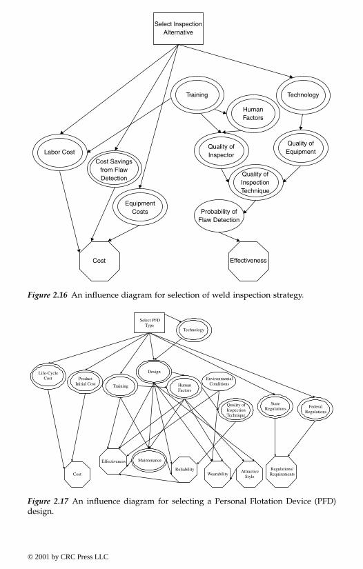
Figure 2.16 An influence diagram for selection of weld inspection strategy.
Figure 2.17 An influence diagram for selecting a Personal Flotation Device (PFD)design.
Select InspectionAlternative
Labor Cost
Cost Savingsfrom FlawDetection
EquipmentCosts Probability of
Flaw Detection
Cost Effectiveness
Training
HumanFactors
Technology
Quality ofInspector
Quality ofInspectionTechnique
Quality ofEquipment
Cost
Effectiveness
ProductInitial Cost
Life-CycleCost
Training HumanFactors
Quality ofInspectionTechnique
StateRegulations
Technology
FederalRegulations
EnvironmentalConditions
Select PFDType
ReliabilityWearability
AttractiveStyle
Design
Maintenance
Regulations/Requirements
© 2001 by CRC Press LLC
of these objectives. However, in order to develop a control system for aconstruction activity, this activity has to be suitably defined depending onits nature and methods of control. Hierarchical control systems were deter-mined to be suitable for construction activities (Abraham et al., 1989). Thus,the hierarchical nature of a construction activity needs to be emphasized.The generalized system definition as discussed in this section can be usedfor this purpose. The hierarchical system classification enables the decom-position of the overall construction activity into subsystems that representthe different processes involved in each activity. Then, each process couldbe decomposed into tasks that are involved in performing the process. There-fore, a breakdown needed for a hierarchical control system is obtained. Inthis section, basic concepts of system identification and definitions are intro-duced, together with some additional concepts that could be used in mod-eling and solving problems in engineering and sciences. Construction activ-ities are modeled and discussed using the methods presented in this sectionin a systems framework for the purpose of demonstration. The knowledgesystem is upgraded throughout the course of the coverage in this sectionfrom one system level to the next level in order to illustrate the use of thedeveloped concepts for controlling construction activities.
2.3.2 Knowledge and information hierarchy
The definition of a system is commonly considered the first step in an overallmethodology formulated for achieving a set of objectives (Chestnut, 1965;Hall, 1962 and 1989; Klir, 1969 and 1985; Wilson, 1984). The definition of asystem can be interpreted in many ways as discussed in Section 2.2; how-ever, herein a universal definition is used as an arrangement of elementswith some important properties and interrelations among them. In order tointroduce a comprehensive definition of a system, a more specific descrip-tion is required based on several main knowledge levels (Klir, 1969 and1985). Further classifications of systems are possible within each level usingmethodological distinctions based on, for example, their nature as natural,designed, human activity, and social and cultural (Wilson, 1984). Chestnut(1965) and Hall (1962 and 1989) provided hierarchical formulations of sys-tems based on available information and its degree of detail. Klir (1969 and1985) introduced a set approach for the system definition problem that wascriticized by Hall (1989) because of its inability to express the properties ofthe overall system, knowing the qualities of its elements. However, forconstruction activities, the set approach is suitable for representing thevariables of the problem. The ability to infer information about the overallsystem, knowing the behavior of its components, can be dealt with usingspecial techniques as discussed by Klir (1985). Once a system is defined,the next step is to define its environment (Chestnut, 1965; Hall, 1962 and1989; Klir, 1969 and 1985; Wilson, 1984). The environment is defined aseverything within a certain universe that is not included in the system. Hall(1989) introduced an interesting notion within systems thinking that allows
© 2001 by CRC Press LLC
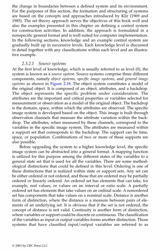
the change in boundaries between a defined system and its environment.For the purposes of this section, the formation and structuring of systemsare based on the concepts and approaches introduced by Klir (1969 and1985). The set theory approach serves the objectives of this book well andalso the examples presented in this chapter on defining a control systemfor construction activities. In addition, the approach is formulated in anonspecific general format and is well suited for computer implementation.In the following sections, knowledge and an example control system aregradually built up in successive levels. Each knowledge level is discussedin detail together with any classifications within each level and an illustra-tive example.
2.3.2.1 Source systemsAt the first level of knowledge, which is usually referred to as level (0), thesystem is known as a source system. Source systems comprise three differentcomponents, namely object systems, specific image systems, and general imagesystems as shown in Figure 2.18. The object system constitutes a model ofthe original object. It is composed of an object, attributes, and a backdrop.The object represents the specific problem under consideration. Theattributes are the important and critical properties or variables selected formeasurement or observation as a model of the original object. The backdropis the domain, space, within which the attributes are observed. The specificimage system is developed based on the object. This image is built throughobservation channels that measure the attribute variation within the back-drop. The attributes, when measured by these channels, correspond to thevariables in the specific image system. The attributes are measured withina support set that corresponds to the backdrop. The support can be time,space, or population. Combinations of two or more of these supports arealso possible.
Before upgrading the system to a higher knowledge level, the specificimage system can be abstracted into a general format. A mapping functionis utilized for this purpose among the different states of the variables to ageneral state set that is used for all the variables. There are some method-ological distinctions that could be defined in this level. Ordering is one ofthese distinctions that is realized within state or support sets. Any set canbe either ordered or not ordered, and those that are ordered may be partiallyordered or linearly ordered. An ordered set has elements that can take, forexample, real values, or values on an interval or ratio scale. A partiallyordered set has elements that take values on an ordinal scale. A nonorderedset has components that take values on a nominal scale. Distance is anotherform of distinction, where the distance is a measure between pairs of ele-ments of an underlying set. It is obvious that if the set is not ordered, theconcept of distance is not valid. Continuity is another form of distinction,where variables or support could be discrete or continuous. The classificationof the variables as input or output variables forms another distinction. Thosesystems that have classified input/output variables are referred to as
© 2001 by CRC Press LLC

directed systems; otherwise they are referred to as neutral systems. The lastdistinctions that could be realized in this level are related to the observationchannels, which could be classified as crisp or fuzzy. Figure 2.19 summarizesmethodological distinctions realized in the first level of knowledge. It shouldbe noted that any variation or change in the methodological distinctions ofa certain system does not affect its knowledge level.
Figure 2.18 Source system components.
General Image System
Specific Image System
Object System:object, attributes and a backdrop
Abstraction
InterpretationChannels
Exemplification
ObservationChannels
To Higher SystemLevels
Level (0) Source System
Abs
trac
tion
Inte
rpre
tatio
n
Real System
Analyst orSystem Engineer
© 2001 by CRC Press LLC

Example 2.6 A source system for construction activities
For the purpose of illustration, the construction activities of concrete place-ment are considered and their knowledge level upgraded throughout thecourse of this section. The first step in defining the system for these con-struction activities is to identify a goal such as construction control by safelyplacing high quality concrete efficiently and precisely. This goal can bedefined through some properties or attributes of interest that can include,for example, safety, quality, productivity, and precision. Considering onlytwo attributes of construction activities, i.e., safety and quality, the variablesor factors that affect those attributes should be identified. Only two variablesare assumed to affect the safety attribute. These variables could be quanti-tatively or qualitatively defined depending on their nature. For qualitativevariables, fuzzy set theory is used in defining the potential states togetherwith a suitable observation channel that yields a quantitative equivalent foreach state (Klir, 1985; Klir and Folger, 1988; Zimmerman, 1985). As an exam-ple for this type of variable, labor experience (v1) is considered. This variableis assumed to have four potential states, namely, fair, good, moderate, andexcellent. These linguistic measures can be defined using fuzzy sets. Usinga scale of 0 to 10 for the level of experience, these measures can be definedas shown in Figure 2.20. The vertical axis in the figure represents the degree
Figure 2.19 Methodological distinctions of source systems.
Source System
Ordering
WithoutOrdering
PartialOrdering
LinearOrdering
Distance
NotRecognized
Recognized
Continuity
Discrete Continuous
Variable Classification(input/output)
Directed Neutral
ObservationChannels
Crisp Fuzzy
© 2001 by CRC Press LLC
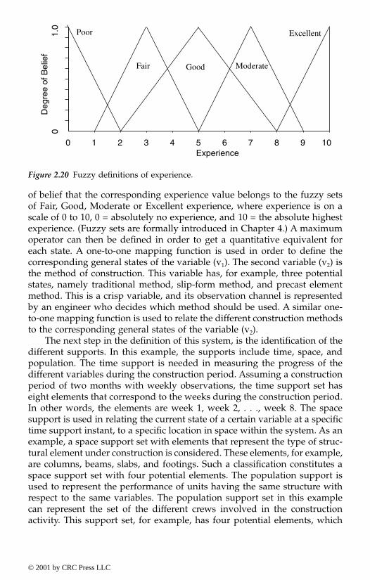
of belief that the corresponding experience value belongs to the fuzzy setsof Fair, Good, Moderate or Excellent experience, where experience is on ascale of 0 to 10, 0 = absolutely no experience, and 10 = the absolute highestexperience. (Fuzzy sets are formally introduced in Chapter 4.) A maximumoperator can then be defined in order to get a quantitative equivalent foreach state. A one-to-one mapping function is used in order to define thecorresponding general states of the variable (v1). The second variable (v2) isthe method of construction. This variable has, for example, three potentialstates, namely traditional method, slip-form method, and precast elementmethod. This is a crisp variable, and its observation channel is representedby an engineer who decides which method should be used. A similar one-to-one mapping function is used to relate the different construction methodsto the corresponding general states of the variable (v2).
The next step in the definition of this system, is the identification of thedifferent supports. In this example, the supports include time, space, andpopulation. The time support is needed in measuring the progress of thedifferent variables during the construction period. Assuming a constructionperiod of two months with weekly observations, the time support set haseight elements that correspond to the weeks during the construction period.In other words, the elements are week 1, week 2, . . ., week 8. The spacesupport is used in relating the current state of a certain variable at a specifictime support instant, to a specific location in space within the system. As anexample, a space support set with elements that represent the type of struc-tural element under construction is considered. These elements, for example,are columns, beams, slabs, and footings. Such a classification constitutes aspace support set with four potential elements. The population support isused to represent the performance of units having the same structure withrespect to the same variables. The population support set in this examplecan represent the set of the different crews involved in the constructionactivity. This support set, for example, has four potential elements, which
Figure 2.20 Fuzzy definitions of experience.
0 1 2 3 4 5 6 7 8 9 10Experience
Deg
ree
of B
elie
f0
1.0 Poor
Fair Good Moderate
Excellent
© 2001 by CRC Press LLC
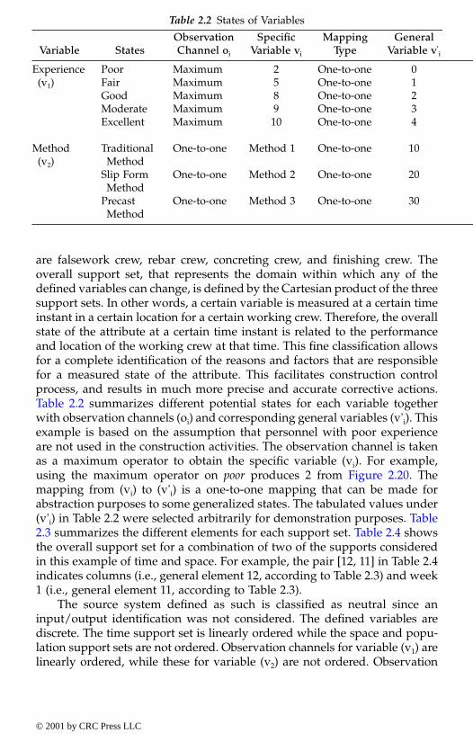
are falsework crew, rebar crew, concreting crew, and finishing crew. Theoverall support set, that represents the domain within which any of thedefined variables can change, is defined by the Cartesian product of the threesupport sets. In other words, a certain variable is measured at a certain timeinstant in a certain location for a certain working crew. Therefore, the overallstate of the attribute at a certain time instant is related to the performanceand location of the working crew at that time. This fine classification allowsfor a complete identification of the reasons and factors that are responsiblefor a measured state of the attribute. This facilitates construction controlprocess, and results in much more precise and accurate corrective actions.Table 2.2 summarizes different potential states for each variable togetherwith observation channels (oi) and corresponding general variables (v'i). Thisexample is based on the assumption that personnel with poor experienceare not used in the construction activities. The observation channel is takenas a maximum operator to obtain the specific variable (vi). For example,using the maximum operator on poor produces 2 from Figure 2.20. Themapping from (vi) to (v'i) is a one-to-one mapping that can be made forabstraction purposes to some generalized states. The tabulated values under(v'i) in Table 2.2 were selected arbitrarily for demonstration purposes. Table2.3 summarizes the different elements for each support set. Table 2.4 showsthe overall support set for a combination of two of the supports consideredin this example of time and space. For example, the pair [12, 11] in Table 2.4indicates columns (i.e., general element 12, according to Table 2.3) and week1 (i.e., general element 11, according to Table 2.3).
The source system defined as such is classified as neutral since aninput/output identification was not considered. The defined variables arediscrete. The time support set is linearly ordered while the space and popu-lation support sets are not ordered. Observation channels for variable (v1) arelinearly ordered, while these for variable (v2) are not ordered. Observation
Table 2.2 States of Variables
Variable StatesObservation Channel oi
SpecificVariable vi
MappingType
GeneralVariable v'
i
Experience(v1)
PoorFairGoodModerateExcellent
MaximumMaximumMaximumMaximumMaximum
258910
One-to-oneOne-to-oneOne-to-oneOne-to-oneOne-to-one
01234
Method(v2)
Traditional Method
Slip Form Method
Precast Method
One-to-one
One-to-one
One-to-one
Method 1
Method 2
Method 3
One-to-one
One-to-one
One-to-one
10
20
30
© 2001 by CRC Press LLC

channels for variable (v1) are fuzzy, while those for variable (v2) are crisp.Figure 2.21 shows a block diagram of this source system.
2.3.2.2 Data systemsThe second level of a hierarchical system classification is the data system,which includes a source system together with actual data introduced in theform of states of variables for each attribute. The actual states of the variablesat the different support instances yield the overall states of the attributes.Special functions and techniques are used to infer information regarding anattribute, based on the states of the variables representing it. A formal def-inition of a data system could be expressed as follows:
D = {S, a} (2.2)
Table 2.3 Elements of the Different Support Sets
Support Specific Element Mapping Type General Element
Time week 1week 2week 3week 4week 5week 6week 7week 8
One-to-oneOne-to-oneOne-to-oneOne-to-oneOne-to-oneOne-to-oneOne-to-oneOne-to-one
1121314151617181
Space ColumnsBeamsSlabsFootings
One-to-oneOne-to-oneOne-to-oneOne-to-one
12223242
Population Falsework CrewRebar CrewConcreting CrewFinishing Crew
One-to-oneOne-to-oneOne-to-oneOne-to-one
13233343
Table 2.4 The Overall Support Set of Time and Space
Space
Time (Week)
Week (11)
Week (21)
Week (31)
Week (41)
Week (51)
Week (61)
Week (71)
Week (81)
Columns (12)Beams (22)Slabs (32)Footings (42)
[12, 11][22, 11][32, 11][42, 11]
[12, 21][22, 21][32, 21][42, 21]
[12, 31][22, 31][32, 31][42, 31]
[12, 41][22, 41][32, 41][42, 41]
[12, 51][22, 51][32, 51][42, 51]
[12, 61][22, 61][32, 61][42, 61]
[12, 71][22, 71][32, 71][42, 71]
[12, 81][22, 81][32, 81][42, 81]
© 2001 by CRC Press LLC
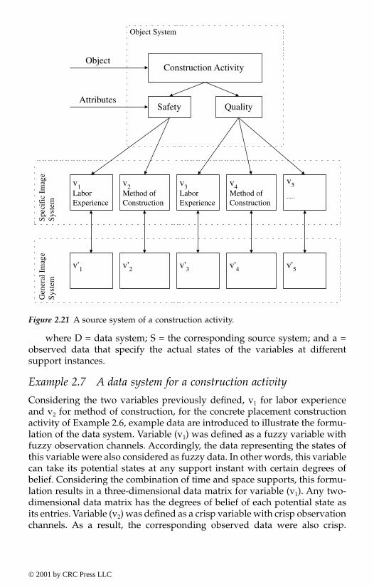
where D = data system; S = the corresponding source system; and a =observed data that specify the actual states of the variables at differentsupport instances.
Example 2.7 A data system for a construction activity
Considering the two variables previously defined, v1 for labor experienceand v2 for method of construction, for the concrete placement constructionactivity of Example 2.6, example data are introduced to illustrate the formu-lation of the data system. Variable (v1) was defined as a fuzzy variable withfuzzy observation channels. Accordingly, the data representing the states ofthis variable were also considered as fuzzy data. In other words, this variablecan take its potential states at any support instant with certain degrees ofbelief. Considering the combination of time and space supports, this formu-lation results in a three-dimensional data matrix for variable (v1). Any two-dimensional data matrix has the degrees of belief of each potential state asits entries. Variable (v2) was defined as a crisp variable with crisp observationchannels. As a result, the corresponding observed data were also crisp.
Figure 2.21 A source system of a construction activity.
Construction Activity
Safety Quality
Object
Object System
v1LaborExperience
Spec
ific
Im
age
Syst
em
Attributes
v2Method ofConstruction
v3LaborExperience
v4Method ofConstruction
v5
.....
v'1
Gen
eral
Im
age
Syst
em
v'2 v'3 v'4 v'5
© 2001 by CRC Press LLC
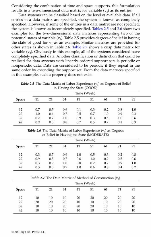
Considering the combination of time and space supports, this formulationresults in a two-dimensional data matrix for variable (v2) as its entries.
Data systems can be classified based on the level of available data. If allentries in a data matrix are specified, the system is known as completelyspecified. However, if some of the entries in a data matrix are not specified,the system is known as incompletely specified. Tables 2.5 and 2.6 show twoexamples for the two-dimensional data matrices representing two of thepotential states of variable (v1). Table 2.5 provides degrees of belief in havingthe state of good for v1 as an example. Similar matrices are provided forother states as shown in Table 2.6. Table 2.7 shows a crisp data matrix forvariable (v2). Obviously in this example, all of the systems considered havecompletely specified data. Another classification or distinction that could berealized for data systems with linearly ordered support sets is periodic ornonperiodic data. Data are considered to be periodic if they repeat in thesame order by extending the support set. From the data matrices specifiedin this example, such a property does not exist.
Table 2.5 The Data Matrix of Labor Experience (v1) as Degrees of Beliefin Having the State (GOOD)
Space
Time (Week)
11 21 31 41 51 61 71 81
12223242
0.71.00.20.9
0.50.40.70.5
0.60.71.00.8
0.10.50.90.7
0.30.70.30.5
0.21.00.50.2
0.80.91.00.1
1.00.30.60.3
Table 2.6 The Data Matrix of Labor Experience (v1) as Degreesof Belief in Having the State (MODERATE)
Space
Time (Week)
11 21 31 41 51 61 71 81
12223242
0.30.90.30.3
0.70.50.90.5
0.90.71.00.7
1.00.60.81.0
0.51.00.20.6
0.30.90.70.8
0.20.50.90.4
0.80.61.00.2
Table 2.7 The Data Matrix of Method of Construction (v2)
Space
Time (Week)
11 21 31 41 51 61 71 81
12223242
10201010
10201010
10202010
20102010
20102010
20101010
20201010
20201010
© 2001 by CRC Press LLC
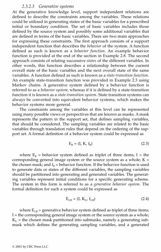
2.3.2.3 Generative systemsAt the generative knowledge level, support independent relations aredefined to describe the constraints among the variables. These relationscould be utilized in generating states of the basic variables for a prescribedinitial or boundary condition. The set of basic variables includes thosedefined by the source system and possibly some additional variables thatare defined in terms of the basic variables. There are two main approachesfor expressing these constraints. The first approach consists of a supportindependent function that describes the behavior of the system. A functiondefined as such is known as a behavior function. An example behaviorfunction is provided at the end of the section in Example 2.8. The secondapproach consists of relating successive states of the different variables. Inother words, this function describes a relationship between the currentoverall state of the basic variables and the next overall state of the samevariables. A function defined as such is known as a state-transition function.An example state-transition function was provided in Example 2.3 usingMarkov chains. A generative system defined by a behavior function isreferred to as a behavior system, whereas if it is defined by a state-transitionfunction it is known as a state-transition system. State transition systems canalways be converted into equivalent behavior systems, which makes thebehavior systems more general.
The constraints among the variables at this level can be representedusing many possible views or perspectives that are known as masks. A maskrepresents the pattern in the support set, that defines sampling variables,that should be considered. The sampling variables are related to the basicvariables through translation rules that depend on the ordering of the sup-port set. A formal definition of a behavior system could be expressed as
EB = (I, K, fB) (2.3)
where EB = behavior system defined as triplet of three items; I = thecorresponding general image system or the source system as a whole; K =the chosen mask; and fB = behavior function. If the behavior function is usedto generate data or states of the different variables, the sampling variablesshould be partitioned into generating and generated variables. The generat-ing variables represent initial conditions for a specific generating scheme.The system in this form is referred to as a generative behavior system. Theformal definition for such a system could be expressed as
EGB = (I, KG, fGB) (2.4)
where EGB = generative behavior system defined as triplet of three items;I = the corresponding general image system or the source system as a whole;KG = the chosen mask partitioned into submasks, namely a generating sub-mask which defines the generating sampling variables, and a generated
© 2001 by CRC Press LLC
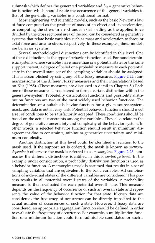
submask which defines the generated variables; and fGB = generative behav-ior function which should relate the occurrence of the general variables tothat of the generating variables in a conditional format.
Most engineering and scientific models, such as the basic Newton’s lawof force computed as the product of mass of an object and its acceleration,or computing the stress in a rod under axial loading as the applied forcedivided by the cross sectional area of the rod, can be considered as generativesystems that relate basic variables such as mass and acceleration to force, oraxial force and area to stress, respectively. In these examples, these modelsare behavior systems.
Several methodological distinctions can be identified in this level. Oneof these distinctions is the type of behavior function used. For nondetermin-istic systems where variables have more than one potential state for the samesupport instant, a degree of belief or a probability measure to each potentialstate in the overall state set of the sampling variables should be assigned.This is accomplished by using any of the fuzzy measures. Figure 2.22 sum-marizes some of the different fuzzy measures and their interrelations basedon Klir (1985). (These measures are discussed in detail in Chapter 5.) Eachone of these measures is considered to form a certain distinction within thegenerative system. Probability distribution functions and possibility distri-bution functions are two of the most widely used behavior functions. Thedetermination of a suitable behavior function for a given source system,mask, and data is not an easy task. Potential behavior functions should meeta set of conditions to be satisfactorily accepted. These conditions should bebased on the actual constraints among the variables. They also relate to thedegree of generative uncertainty and complexity of the behavior system. Inother words, a selected behavior function should result in minimum dis-agreement due to constraints, minimum generative uncertainty, and mini-mum complexity.
Another distinction at this level could be identified in relation to themask used. If the support set is ordered, the mask is known as memory-dependent; otherwise the mask is referred to as memoryless. Figure 2.23 sum-maries the different distinctions identified in this knowledge level. In theexample under consideration, a probability distribution function is used asa behavior function. A memoryless mask is assumed that results in a set ofsampling variables that are equivalent to the basic variables. All combina-tions of individual states of the different variables are considered. This pro-cess results in all potential overall states of the variables. A probabilitymeasure is then evaluated for each potential overall state. This measuredepends on the frequency of occurrence of such an overall state and repre-sents the value of the behavior function for that state. If crisp data areconsidered, the frequency of occurrence can be directly translated to theactual number of occurrences of such a state. However, if fuzzy data areconsidered, an appropriate aggregation function should be defined in orderto evaluate the frequency of occurrence. For example, a multiplication func-tion or a minimum function could form admissible candidates for such a
© 2001 by CRC Press LLC
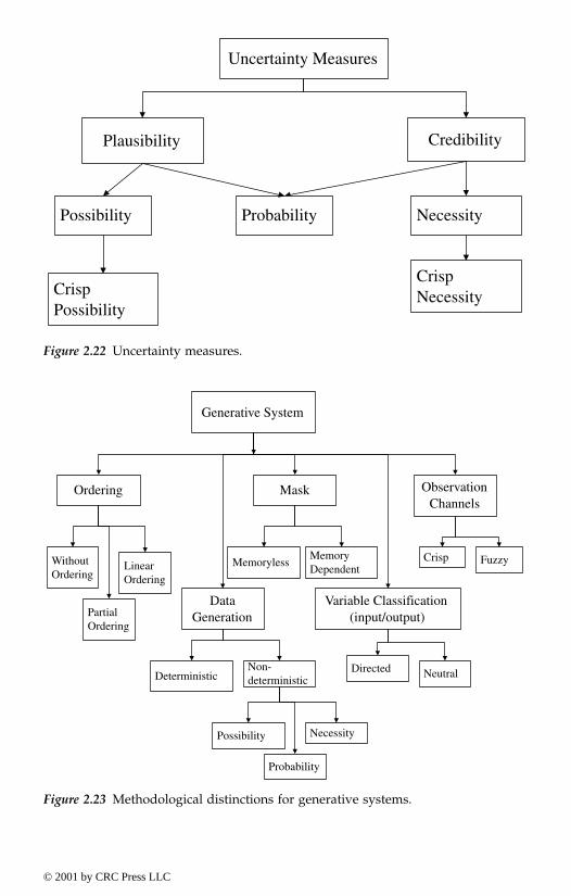
Figure 2.22 Uncertainty measures.
Figure 2.23 Methodological distinctions for generative systems.
Uncertainty Measures
Plausibility
Possibility
Credibility
CrispPossibility
Probability Necessity
CrispNecessity
Generative System
Ordering
WithoutOrdering
PartialOrdering
LinearOrdering
DataGeneration
DeterministicNon-deterministic
Mask
MemorylessMemoryDependent
Variable Classification(input/output)
Directed Neutral
ObservationChannels
Crisp Fuzzy
Possibility
Probability
Necessity
© 2001 by CRC Press LLC

task. These aggregation functions should be applied to the degrees of beliefof the individual states of the different variables, which yield an overalldegree of belief for each overall state. The sum of the degrees of belief of thedifferent occurrences for the same overall state represents a measure for thelikelihood of occurrence of that state. The corresponding probability of occur-rence of each overall state is then calculated as the ratio of the likelihood ofoccurrence of such a state and the sum of all likelihoods of occurrence. Ingeneral, the problem of defining an acceptable behavior function starts withthe determination of all the potential masks. A behavior function is thenevaluated for each proposed mask as previously described. One behaviorfunction should then be chosen based on the three properties mentionedearlier, namely minimum disagreement, minimum generative uncertainty,and minimum complexity.
Example 2.8 A generative system for a construction activity
A memoryless mask was chosen in this example for illustration purposes.In Table 2.8, labor experience variable (v1) was defined as a fuzzy variablethat can take state (1) at different support instances with the degrees of beliefshown in the table. This state was accompanied by state (10) for constructionmethod variable (v2) as shown in the table. Accordingly, the overall state(C1) = (1, 10) has support-variant degrees of belief. Using a minimum oper-ator, for example, as an aggregation function, the degree of belief of state(C1) can be calculated at the different support instants as shown in Table 2.8.In other words, the degree of belief of the combination of states (1) and (10)is the minimum of the two degrees of belief of the separate states. It shouldbe noted that since variable (v2) is a crisp variable, its degree of belief wastaken to be one at any support instant. The likelihood of occurrence of eachoverall state (C1) was then calculated as follows:
Nc = (2.5)
where Nc = likelihood of occurrence; ds,t = aggregated degree of belief ofstate(s) at support instant (t); and the summation was performed over thesupport instances. The corresponding probability of overall state (C1) is thencalculated using the following formula (Klir, 1969 and 1985):
fB(Cl) = (2.6)
where fB(C1) = probability of having state (C1) which corresponds to the valueof the behavior function for that state; Nc = likelihood of occurrence of
ds t,allt∑
Nc
Ncallc∑--------------
© 2001 by CRC Press LLC

Table 2.8 A Behavior Function Evaluation for Variables (v1) and (v2)
Overall State (Ci)
Variable (v1) Variable (v2) Degree of Belief of Overall
State (C)
Likelihood of Occurrence
(Nc)
Behavior Function
(fB)StateDegree of
Belief StateDegree of
Belief
C1 (1, 10) 1111
0.80.70.50.3
10101010
1111
0.80.70.50.3 2.3 0.354
C2 (3, 10) 333
0.40.70.6
101010
111
0.40.60.7 1.7 0.262
C3 (2, 10) 222
0.50.80.9
101010
111
0.50.80.9 2.2 0.338
C4 (0, 10) 00
0.20.1
1010
11
0.20.1 0.3 0.046
© 2001 by C
RC
Press LL
C

state (C1); and the summation was performed over all the overall states.There are other expressions defined in the literature for the calculation ofprobabilities or possibilities based on fuzzy and crisp data (Ayyub andMcCuen, 1998; Ang and Tang, 1975; Klir, 1985). The expressions providedby Equations 2.4 and 2.5 were chosen for illustration purposes. The resultingprobabilities (fB) for selected potential overall states are shown in Table 2.8.
A state transition system can be expressed as
En = (I, K, fn) (2.7)
where En = a state-transition system; I = the corresponding generalimage system; K = the chosen mask; and fn = the state-transition function.An important interpretation of the state transition concept in constructionis the state table approach as used by Abraham et al. (1989). The statetable format could be viewed as a state-transition function in a feedbackcontrol framework. Table 2.9 shows an example of such a table thatdescribes the process of giving some command, the current state of acertain variable, the next state for the same variable, and a feedbackinformation for control purposes. The main concept in this framework isthe relationship developed through the table, between the consecutivestates of the different variables. This support-independent relationshipbetween the successive states of the different variables represents a state-transition function. Figure 2.24 shows a block diagram of the definedgenerative system. It should be emphasized here that although variables1 and 2 for attribute 1 have the same names as variables 3 and 4 forattribute 2, they would not necessarily take the same values. In otherwords, the same variables have different impacts on different attributesaccording to the nature of each attribute.
Table 2.9 A State Table Format (Abraham 1989)
Command State Feedback Next State Output Report
Place concrete for a founda-tion
Formswithoutconcrete
Concrete overflow
Structural member
Concrete member
Concrete quantities
Place concrete for a column
Formswithoutconcrete
Concrete overflow
Structural member
Concrete member
Concrete quantities
Place concrete for a beam
Formswithoutconcrete
Concrete overflow
Structural member
Concrete member
Concrete quantities
Place concrete for a slab
Formswithoutconcrete
Concrete overflow
Structural member
Concrete member
Concrete quantities
© 2001 by CRC Press LLC

2.3.2.4 Structure systemsStructure systems are sets of smaller systems or subsystems. The subsystemscould be source, data, or generative systems. These subsystems may becoupled due to having common variables or due to interaction in some otherform. A formal definition of a structure system could be expressed as follows:
SEB = {(Vi, EBi), for all i ∈ e} (2.8)
where SEB = structure system whose elements are behavior systems; Vi
= the set of sampling variables for the element of the behavior system; EBi
= ith behavior system; and e = the total number of elements or subsystemsin the structure system with all i that belong to e, i.e., for all i ∈ e.
Example 2.9 A structure system for a construction activity
In the construction example, the construction activity is viewed as a structuresystem. The construction activity consists of a number of processes thatshould be accomplished. These processes depend on each other in somemanner. Considering concrete placement as a construction activity, the dif-ferent processes involved include falsework construction, rebar placement,concrete pouring, and concrete finishing. These processes represent interre-
Figure 2.24 A generative system for a construction activity.
Construction Activity{Concrete Placement}
Attribute 1{Safety}
Variable 1{LaborExperience}
Attribute 2{Quality}
Variable 2{Method ofConstruction}
Variable 3{LaborExperience}
Variable 4{Method ofConstruction}
Variable 5{Method ofConstruction}
DATA
ORBehavior FunctionState-Transition
Function
© 2001 by CRC Press LLC
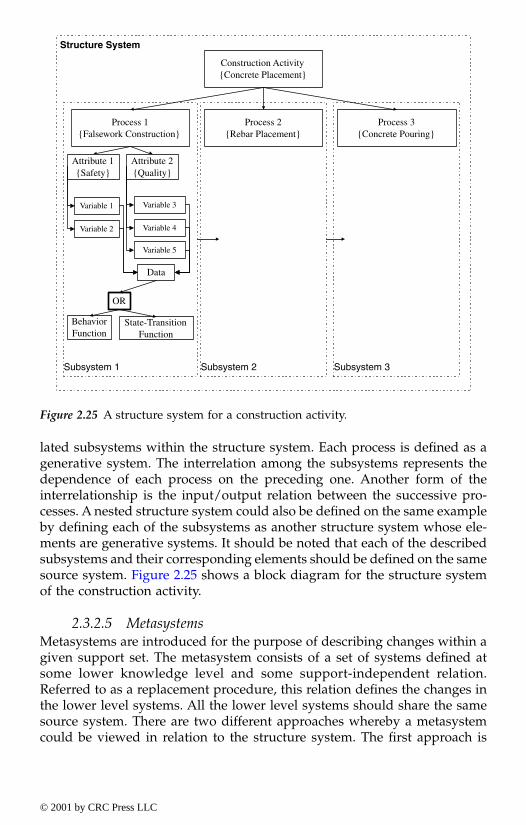
lated subsystems within the structure system. Each process is defined as agenerative system. The interrelation among the subsystems represents thedependence of each process on the preceding one. Another form of theinterrelationship is the input/output relation between the successive pro-cesses. A nested structure system could also be defined on the same exampleby defining each of the subsystems as another structure system whose ele-ments are generative systems. It should be noted that each of the describedsubsystems and their corresponding elements should be defined on the samesource system. Figure 2.25 shows a block diagram for the structure systemof the construction activity.
2.3.2.5 MetasystemsMetasystems are introduced for the purpose of describing changes within agiven support set. The metasystem consists of a set of systems defined atsome lower knowledge level and some support-independent relation.Referred to as a replacement procedure, this relation defines the changes inthe lower level systems. All the lower level systems should share the samesource system. There are two different approaches whereby a metasystemcould be viewed in relation to the structure system. The first approach is
Figure 2.25 A structure system for a construction activity.
Construction Activity{Concrete Placement}
Process 1{Falsework Construction}
Process 2{Rebar Placement}
Process 3{Concrete Pouring}
Attribute 1{Safety}
Attribute 2{Quality}
Variable 1
Variable 2
Variable 3
Variable 4
Variable 5
Data
OR
BehaviorFunction
State-TransitionFunction
Subsystem 1 Subsystem 2 Subsystem 3
Structure System
© 2001 by CRC Press LLC

introduced by defining the system as a structure metasystem. Consideringthe construction example, the construction activity is defined as a structuresystem whose elements are metasystems. Each metasystem represents thechange in its behavior system. As an example for a concrete placementactivity, the processes include falsework construction, rebar placement, andconcrete pouring. However, in order to represent the actual behavior of thissystem within the overall support set required, the behavior system in thiscase can only be defined using more than one behavior function. Each oneof these functions is valid for only a subset of the overall support set. Statingthe problem in this format, a metasystem should be defined to describe thechange in each one of these subsystems. The replacement procedure isrequired in order to decide which behavior function should be used. Thisdecision should be taken based on the states of some basic variables specifiedfor this purpose. Referring to the behavior functions previously defined, i.e.,the probability/possibility distributions, more than one distribution mightbe necessary to fit the available date. Each one of these distributions is validwithin a subset of the overall support set. For example, some distributionmight fit variable (v1) for the first month, i.e., four weeks, while a differentdistribution might more appropriately represent the same variable duringthe next four weeks. Thus, a replacement procedure is required in order tocalculate the current time and choose the appropriate distribution that rep-resents the data during this period. Figure 2.26 shows a graphical represen-tation of a metasystem.
The second approach consists of defining a metasystem of a structuresystem whose elements are behavior systems. Applying this concept to theexample under consideration, a metasystem is defined on the constructionactivity that represents a structure system. In other words, the constructionactivity is the structure system with the different processes defined as sub-systems. This structure system changes with time, where time is as an exam-ple support. At some instant of time, falsework construction and rebarreplacement as two subsystems might be in progress, whereas the otherprocesses, i.e., concrete pouring and concrete finishing, might not be startedyet. Therefore, the components of the structure system at this instant of timedo not include the ones that have not been started. This composition wouldprobably be different after some time, where all the processes might be inprogress at the same time. The replacement procedure in this case shouldobserve the change in each process such that the composition of the structuresystem could be defined at any support instant.
2.4 Models for ignorance and uncertainty types2.4.1 Mathematical theories for ignorance types
Systems analysis provides a general framework for modeling and solvingvarious problems and making appropriate decisions. For example, an engi-neering model of an engineering project starts by defining the system includ-
© 2001 by CRC Press LLC
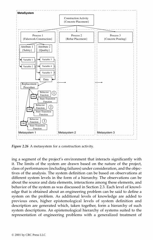
ing a segment of the project’s environment that interacts significantly withit. The limits of the system are drawn based on the nature of the project,class of performances (including failures) under consideration, and the objec-tives of the analysis. The system definition can be based on observations atdifferent system levels in the form of a hierarchy. The observations can beabout the source and data elements, interactions among these elements, andbehavior of the system as was discussed in Section 2.3. Each level of knowl-edge that is obtained about an engineering problem can be said to define asystem on the problem. As additional levels of knowledge are added toprevious ones, higher epistemological levels of system definition anddescription are generated which, taken together, form a hierarchy of suchsystem descriptions. An epistemological hierarchy of systems suited to therepresentation of engineering problems with a generalized treatment of
Figure 2.26 A metasystem for a construction activity.
Construction Activity{Concrete Placement}
Process 1{Falsework Construction}
Process 2{Rebar Placement}
Process 3{Concrete Pouring}
Attribute 1{Safety}
Attribute 2{Quality}
Variable 1
Variable 2
Variable 3
Variable 4
Variable 5
Data
BehaviorFunction
State-TransitionFunction
Metasystem 1 Metasystem 2 Metasystem 3
MetaSystem
OR
ReplacementProcedure
BehaviorFunction
State-TransitionFunction
OR
BehaviorFunction
State-TransitionFunction
OR
1
2
3
© 2001 by CRC Press LLC
uncertainty can provide realistic assessments of systems (Klir, 1985; Klir andFolger, 1988).
Chapter 1 deals with knowledge and ignorance, and their nature, types,and sources as summarized in Figures 1.4 and 1.9, respectively. The nature,types, and sources of knowledge were examined by philosophers, scientists,and engineers as provided in Chapter 1, whereas ignorance has received lessattention. However, interest in analyzing and modeling uncertainty andignorance was started by the works of Zadeh (1965 and 1978), Dempster(1976a and 1976b), Shafer (1976), Sugeno (1974 and 1977), Klir and Folger(1988), Pawlak (1991), and Smithson (1989) by suggesting various modelsand theories for representing ignorance categories that are of the consciousignorance types. Table 2.10 maps various theories that are suitable for igno-rance modeling; however, in solving problems in engineering and sciencethat involve several ignorance types, combinations of these theories areneeded. Each problem might require a mix of theories that most appropri-ately and effectively models its ignorance content.
According to Table 2.10, classical sets theory can effectively deal withambiguity by modeling nonspecificity, whereas fuzzy and rough sets can beused to model vagueness, coarseness, and simplifications. The theories ofprobability and statistics are commonly used to model randomness andsampling uncertainty. Bayesian methods can be used to combine randomnessor sampling uncertainty with subjective information that can be viewed asa form of simplification. Ambiguity, as an ignorance type, forms a basis forrandomness and sampling, hence its cross-shading in the table with classicalsets, probability, statistics, and Bayesian methods. Inaccuracy, as an igno-rance type that can be present in many problems, is cross-shaded in the tablewith probability, statistics, and Bayesian methods. The theories of evidence,possibility, and monotone measure can be used to model confusion, conflict,and vagueness. Interval analysis can be used to model vagueness and sim-plification, whereas interval probabilities can be used to model randomnessand simplification.
2.4.2 Information uncertainty in engineering systems
2.4.2.1 Abstraction and modeling of engineering systemsUncertainty modeling and analysis in engineering started with the employ-ment of safety factors using deterministic analysis, then was followed byprobabilistic analysis with reliability-based safety factors. Uncertainty inengineering was traditionally classified into objective and subjective types.The objective types included the physical, statistical, and modeling sourcesof uncertainty. The subjective types were based on lack of knowledge andexpert-based assessment of engineering variables and parameters. This clas-sification was still deficient in completely covering the entire nature of uncer-tainty. The difficulty in completely modeling and analyzing uncertaintystems from its complex nature and its invasion of almost all epistemologicallevels of a system by varying degrees, as discussed in Chapter 1.
© 2001 by CRC Press LLC
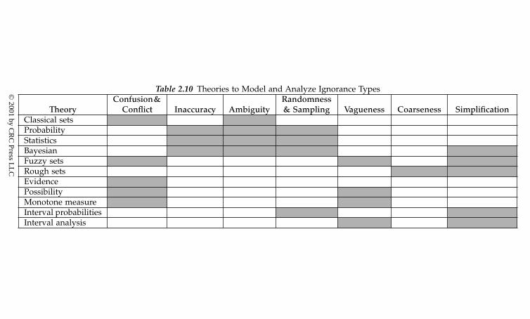
Table 2.10 Theories to Model and Analyze Ignorance Types
TheoryConfusion &
Conflict Inaccuracy AmbiguityRandomness& Sampling Vagueness Coarseness Simplification
Classical setsProbabilityStatisticsBayesianFuzzy sets Rough setsEvidencePossibilityMonotone measureInterval probabilitiesInterval analysis
© 2001 by C
RC
Press LL
C
Engineers can deal with information for the purpose of system analysisand design. Information in this case is classified, sorted, analyzed, and usedto predict system attributes, variables, parameters, and performances. How-ever, it can be more difficult to classify, sort, and analyze the uncertainty inthis information and use it to assess uncertainties in our predictions.
Uncertainties in engineering systems can be mainly attributed to ambi-guity, likelihood, approximations, and inconsistency in defining the archi-tecture, variables, parameters and governing prediction models for the sys-tems. The ambiguity component comes from either not fully identifyingpossible outcomes or incorrectly identifying possible outcomes. Likelihoodbuilds on the ambiguity of defining all the possible outcomes by introducingprobabilities to represent randomness and sampling. Therefore, likelihoodincludes the sources (1) physical randomness and (2) statistical uncertaintydue to the use of sampled information to estimate the characteristics of thepopulation parameters. Simplifications and assumptions, as components ofapproximations, are common in engineering due to the lack of knowledgeand the use of analytical and prediction models, simplified methods, andidealized representations of real performances. Approximations also includevagueness and coarseness. The vagueness-related uncertainty is due tosources that include (1) the definition of some parameters, e.g., structuralperformance (failure or survival), quality, deterioration, skill and experienceof construction workers and engineers, environmental impact of projects,conditions of existing structures using linguistic measures; (2) human factors;and (3) defining the interrelationships among the parameters of the prob-lems, especially for complex systems. The coarseness uncertainty can benoted in simplification models and behavior of systems. Other sources ofignorance include inconsistency with its components of conflict and confu-sion of information and inaccuracies due to, for example, human and orga-nizational errors.
Analysis of engineering systems commonly starts with a definition of asystem that can be viewed as an abstraction of the real system. The abstrac-tion is performed at different epistemological levels (Ayyub, 1992 and 1994).The process of abstraction can be graphically represented as shown in Figure2.27. A resulting model from this abstraction depends largely on the engineer(or analyst) who performed the abstraction, hence on the subjective natureof this process. During the process of abstraction, the engineer needs to makedecisions regarding what aspects should or should not be included in themodel. These aspects are shown in the Figure 2.27. Aspects that areabstracted and not abstracted include the previously identified uncertaintytypes. In addition to the abstracted and nonabstracted aspects, unknownaspects of the system can exist due to blind ignorance, and they are moredifficult to deal with because of their unknown nature, sources, extents, andimpact on the system.
In engineering, it is common to perform uncertainty modeling and anal-ysis of the abstracted aspects of the system with a proper consideration ofthe nonabstracted aspects of a system. The division between abstracted and
© 2001 by CRC Press LLC

nonabstracted aspects can be a division of convenience that is driven by theobjectives of the system modeling, or simplification of the model. However,the unknown aspects of the systems are due to blind ignorance that dependson the knowledge of the analyst and the state of knowledge about the systemin general. The effects of the unknown aspects on the ability of the systemmodel to predict the behavior of the real system can range from none tosignificant.
2.4.2.2 Ignorance and uncertainty in abstracted aspects of a systemEngineers and researchers dealt with the ambiguity and likelihood types ofuncertainty in predicting the behavior and designing engineering systemsusing the theories of probability and statistics and Bayesian methods. Prob-ability distributions were used to model system parameters that are uncer-tain. Probabilistic methods that include reliability methods, probabilisticengineering mechanics, stochastic finite element methods, reliability-baseddesign formats, and other methods were developed and used for this pur-pose. In this treatment, however, a realization was established of the presence
Figure 2.27 Abstraction and ignorance for engineering systems.
Real System
Abs
trac
tion
at s
ever
alep
iste
mol
ogic
al le
vels
.
EngineerorAnalyst
A model of the real system
Abstracted Aspectsof the System
Non-abstracted Aspectsof the System
Unknown Aspectsof the System: Blind
Ignorance
Ambiguity Likelihood Approximation Inconsistency
Vagueness Coarseness
Simplifications
Randomness
Sampling
Confusion
ConflictInaccuracy
Unknowns
IrrelevanceFallacy
Unspecificity
Non-specificity
© 2001 by CRC Press LLC
of the approximations type of uncertainty. Subjective probabilities were usedto deal with this type that are based on mathematics used for the frequency-type of probability. Uniform and triangular probability distributions wereused to model this type of uncertainty for some parameters. The Bayesiantechniques were also used, for example, to deal with combining empiricaland subjective information about these parameters. The underlying distri-butions and probabilities were, therefore, updated. Regardless of the natureof uncertainty in the gained information, similar mathematical assumptionsand tools were used that are based on probability theory.
Approximations arise from human cognition and intelligence. Theyresult in uncertainty in mind-based abstractions of reality. These abstractionsare, therefore, subjective and can lack crispness, they can be coarse in nature,or they might be based on simplifications. The lack of crispness, calledvagueness, is distinct from ambiguity and likelihood in source and naturalproperties. The axioms of probability and statistics are limiting for the propermodeling and analysis of this uncertainty type and are not completely rele-vant, nor completely applicable. The vagueness type of uncertainty in engi-neering systems can be dealt with using appropriately fuzzy set theory(Zadeh, 1965). Fuzzy set theory has been developed by Zadeh (1965, 1968,1973, 1975, 1978) and used by scientists, researchers, and engineers in manyfields. Example applications are provided elsewhere (Kaufmann and Gupta,1985; Kaufmann, 1975). In engineering, the theory was proven to be a usefultool in solving problems that involve the vagueness type of uncertainty. Forexample, civil engineers and researchers started using fuzzy sets and systemsin the early 1970s (Brown, 1979 and 1980; Brown and Yao, 1983). To date,many applications of the theory in engineering were developed. The theoryhas been successfully used in, for example (Ayyub, 1991; Blockley, 1975,1979a, 1979b, 1980; Blockley et al., 1983; Shiraishi and Furuta, 1983; Shiraishiet al., 1985; Yao, 1979, 1980; Yao and Furuta, 1986; Blockley et al., 1975 to1983; Furuta et al., 1985 and 1986; Ishizuka et al., 1981 and 1983; Itoh andItagaki, 1989; Kaneyoshi, 1990; Shiraishi et al., 1983 and 1985; Yao et al. 1979,1980, 1986),
• strength assessment of existing structures and other structural engi-neering applications;
• risk analysis and assessment in engineering;• analysis of construction failures, scheduling of construction activities,
safety assessment of construction activities, decisions during con-struction and tender evaluation;
• the impact assessment of engineering projects on the quality of wild-life habitat;
• planning of river basins;• control of engineering systems;• computer vision; and• optimization based on soft constraints.
© 2001 by CRC Press LLC
Coarseness in information can arise from approximating an unknownrelationship or set by partitioning the universal space with associated belieflevels for the partitioning subsets in representing the unknown relationshipor set (Pawlak, 1991). Such an approximation is based on rough sets asdescribed in Chapter 4. Pal and Skowron (1999) provide background anddetailed information on rough set theory, its applications, and hybrid fuzzy-rough set modeling. Simplifying assumptions are common in developingengineering models. Errors resulting from these simplifications are com-monly dealt with in engineering using bias random variables that areassessed empirically. A system can also be simplified by using knowledge-based if-then rules to represent its behavior based on fuzzy logic and approx-imate reasoning.
2.4.2.3 Ignorance and uncertainty in nonabstracted aspects of a system
In developing a model, an analyst or engineer needs to decide, at the differentlevels of modeling a system, upon the aspects of the system that need to beabstracted and the aspects that need not to be abstracted. The divisionbetween abstracted and nonabstracted aspects can be for convenience or tosimplify the model. The resulting division can depend on the analyst orengineer, as a result of his or her background, and the general state ofknowledge about the system.
The abstracted aspects of a system and their uncertainty models can bedeveloped to account for the nonabstracted aspects of the system to someextent. Generally, this accounting process is incomplete. Therefore, a sourceof uncertainty exists due to the nonabstracted aspects of the system. Theignorance categories and uncertainty types in this case are similar to theprevious case of abstracted aspects of the system. These categories and typesare shown in Figure 2.27.
The ignorance categories and uncertainty types due to the nonabstractedaspects of a system are more difficult to deal with than the uncertainty typesdue to the abstracted aspects of the system. The difficulty can stem from alack of knowledge or understanding of the effects of the nonabstractedaspects on the resulting model in terms of its ability to mimic the real system.Poor judgment or human errors about the importance of the nonabstractedaspects of the system can partly contribute to these uncertainty types, inaddition to contributing to the next category, uncertainty due to theunknown aspects of a system.
2.4.2.4 Ignorance due to unknown aspects of a systemSome engineering failures have occurred because of failure modes that werenot accounted for in the design stages of these systems. The nonaccountingfor the failure modes can be due to (1) blind ignorance, negligence, usingirrelevant information or knowledge, human errors, or organizational errors;or (2) a general state of knowledge about a system that is incomplete. These
© 2001 by CRC Press LLC

unknown system aspects depend on the nature of the system under consid-eration, the knowledge of the analyst, and the state of knowledge about thesystem in general. The nonaccounting of these aspects in the models for thesystem can result in varying levels of impact on the ability of these modelsin mimicking the behavior of the systems. The effects of the unknown aspectson these models can range from none to significant. In this case, the ignorancecategories include wrong information and fallacy, irrelevant information,and unknowns as shown in Figure 2.27.
Engineers dealt with nonabstracted and unknown aspects of a systemby assessing what is commonly called the modeling uncertainty, defined asthe ratio of a predicted system’s variables or parameters (based on the model)to the value of the parameter in the real system. This empirical ratio, whichis called the bias, is commonly treated as a random variable that can consistof objective and subjective components. Factors of safety are intended tosafeguard against failures. This approach of bias assessment is based on twoimplicit assumptions: (1) the value of the variable or parameter for the realsystem is known or can be accurately assessed from historical informationor expert judgment; and (2) the state of knowledge about the real system iscomplete or bounded, and reliable. For some systems, the first assumptioncan be approximately examined through verification and validation, whereasthe second assumption generally cannot be validated.
2.5 System complexityOur most troubling long-range problems, such as economic forecasting andtrade balance, defense systems, and genetic modeling, center on systems ofextraordinary complexity. The systems that host these problems — computernetworks, economics, ecologies, and immune systems — appear to be asdiverse as the problems. Humans as complex, intelligent systems have theability to anticipate the future, learn, and adapt in ways that are not yet fullyunderstood. Engineers and scientists, who study or design systems, have todeal with complexity more often than ever, hence the interest in the field ofcomplexity. Understanding and modeling system complexity can be viewedas a pretext for solving complex scientific and technological problems, suchas finding a cure for the acquired immune deficiency syndrome (AIDS),solving long-term environmental issues, or using genetic engineering safelyin agricultural products. The study of complexity led to, for example, chaosand catastrophe theories. Even if complexity theories would not producesolutions to problems, they can still help us to understand complex systemsand perhaps direct experimental studies. Theory and experiment go handin glove, therefore providing opportunities to make major contributions.
The science of complexity was founded at the Santa Fe Institute by agroup of physicists, economists, mathematicians, and computer scientists thatincluded Nobel Laureates in physics and economics, Murray Gell-Mann andKenneth Arrow, respectively. They noted that scientific modeling and discov-ery tends to emphasize linearity and reductionism, and they consequently
© 2001 by CRC Press LLC

developed the science of complexity based on assumed interconnectivity, co-evolution, chaos, structure, and order to model nature, human social behavior,life, and the universe in unified manners (Waldrop 1992).
Complexity can be classified into two broad categories: (1) complexitywith structure, and (2) complexity without structure. The complexity withstructure was termed organized complexity by Weaver (1948). Organized com-plexity can be observed in a system that involves nonlinear differentialequations with many interactions among a large number of components andvariables that define the system, such as in life, behavioral, social, and envi-ronmental sciences. Such systems are usually nondeterministic in theirnature. Problem solutions related to such models of organized complexitytend to converge to statistically meaningful averages (Klir and Wierman,1999). Advancements in computer technology and numerical methods haveenhanced our ability to obtain such solutions effectively and inexpensively.As a result, engineers design complex systems in simulated environmentsand operations, such as a space mission to a distant planet, and scientistscan conduct numerical experiments involving, for example, nuclear blasts.
In the area of simulation-based design, engineers are using parallel com-puting and physics-based modeling to simulate fire propagation in engineer-ing systems, or the turbulent flow of a jet engine using molecular motionand modeling. These computer and numerical advancements are not limit-less, as the increasing computational requirements lead to what is termedtranscomputational problems capped by the Bremermann’s limit (Bremermann,1962). The nature of such transcomputational problems is studied by thetheory of computational complexity (Garey and Johnson, 1979). The Bremer-mann’s limit was estimated based on quantum theory using the followingproposition (Bremermann, 1962):
“No data processing systems, whether artificial or liv-ing, can process more than 2 × 1047 bits per second pergram of its mass,”
where data processing is defined as transmitting bits over one or severalof a system’s channels. Klir and Folger (1988) provide additional informationon the theoretical basis for this proposition, showing that the maximumprocessing value is to be 1.36 × 1047 bits per second per gram of its mass.Considering a hypothetical computer that has the entire mass of the Earthoperating for a time period equal to an estimated age of the Earth, i.e., 6 × 1027
grams and 1010 years, respectively, with each year containing 3.15 × 10⁷
seconds, this imaginary computer would be able to process 2.57 × 1092 bits,or rounded to the nearest power of ten, 1093 bits, defining the Bremermann’slimit. Many scientific and engineering problems defined with many detailscan exceed this limit. Klir and Folger (1988) provide the examples of patternrecognition and human vision that can easily reach transcomputational lev-els. In pattern recognition, consider a square q × q spatial array defining
© 2001 by CRC Press LLC

n = q2 cells that partition the recognition space. Pattern recognition ofteninvolves color. Using k colors, as an example, the number of possible colorpatterns within the space is kn. In order to stay within the Bremermann’slimit, the following inequality must be met:
kn < 1093 (2.9)
Figure 2.28 shows a plot of this inequality for values of k = 2 to 10 colors.For example using only two colors, a transcomputational state is reached atq > 18 colors. These computations in pattern recognition can be directlyrelated to human vision and the complexity associated with processing infor-mation by the retina of a human eye. According to Klir and Folger (1988), ifwe consider a retina of about one million cells with each cell having onlytwo states, active and inactive, in recognizing an object, modeling the retinain its entirety would require the processing of
21,000,000 = 10300 (2.10)
bits of information, far beyond the Bremermann’s limit.Generally, an engineering system needs to be modeled with a portion
of its environment that interacts significantly with it in order to assess somesystem attributes of interest. The level of interaction with the environmentcan be assessed only subjectively. By increasing the size of the environmentand level of details in a model of the system, the complexity of the systemmodel increases, possibly in a manner that does not have a recognizable orobservable structure. This complexity without structure is more difficult tomodel and deal with in engineering and sciences. By increasing the com-plexity of the system model, our ability to make relevant assessments of the
Figure 2.28 The Bremermann’s limit for pattern recognition.
8
10
12
14
16
18
20
1 3 6 8 10
Number of Colors (n)
Siz
e o
f S
pat
ial F
ield
(q
)
Transcomputational Region
2 4 5 7 9
© 2001 by CRC Press LLC
system’s attributes can diminish. Therefore, there is a tradeoff betweenrelevance and precision in system modeling in this case. Our goal shouldbe to model a system with a sufficient level of detail that can result insufficient precision and can lead to relevant decisions in order to meet theobjective of the system assessment.
Living systems show signs of these tradeoffs between precision andrelevance in order to deal with complexity. The survival instincts of livingsystems have evolved and manifest themselves as processes to cope withcomplexity and information overload. The ability of a living system to makerelevant assessments diminishes with increased information input, as dis-cussed by Miller (1978). Living systems commonly need to process informa-tion in a continuous manner in order to survive. For example, a fish needsto process visual information constantly in order to avoid being eaten byanother fish. When a school of larger fish rushes towards the fish, presentingit with images of threats and dangers, the fish might not be able to processall the information and images become confused. Considering the informa-tion processing capabilities of living systems as input-output black boxes,the input and output to such systems can be measured and plotted in orderto examine such relationships and any nonlinear characteristics that theymight exhibit. Miller (1978) described these relationships for living systemsusing the following hypothesis that was analytically modeled and experi-mentally validated:
As the information input to a single channel of a livingsystem — measured in bits per second — increases,the information output — measured similarly — in-creases almost identically at first but gradually fallsbehind as it approaches a certain output rate, the chan-nel capacity, which cannot be exceeded. The outputthen levels off at that rate, and finally, as the informa-tion input rate continues to go up, the output decreasesgradually towards zero as breakdown or the confusionstate occurs under overload.
The above hypothesis was used to construct families of curves to repre-sent the effects of information input overload, as shown schematically inFigure 2.29. Once the input overload is removed, most living systems recoverinstantly from the overload, and the process is completely reversible; how-ever, if the energy level of the input is much larger than the channel capacity,a living system might not fully recover from this input overload. Livingsystems also adjust the way they process information in order to deal withan information input overload using one or more of the following processesby varying degrees depending on the level of a living system in terms ofcomplexity: (1) omission by failing to transmit information, (2) error bytransmitting information incorrectly, (3) queuing by delaying transmission,(4) filtering by giving priority in processing, (5) abstracting by processing
© 2001 by CRC Press LLC
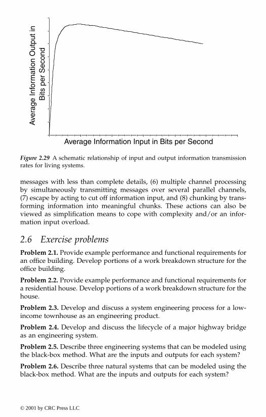
messages with less than complete details, (6) multiple channel processingby simultaneously transmitting messages over several parallel channels,(7) escape by acting to cut off information input, and (8) chunking by trans-forming information into meaningful chunks. These actions can also beviewed as simplification means to cope with complexity and/or an infor-mation input overload.
2.6 Exercise problemsProblem 2.1. Provide example performance and functional requirements foran office building. Develop portions of a work breakdown structure for theoffice building.
Problem 2.2. Provide example performance and functional requirements fora residential house. Develop portions of a work breakdown structure for thehouse.
Problem 2.3. Develop and discuss a system engineering process for a low-income townhouse as an engineering product.
Problem 2.4. Develop and discuss the lifecycle of a major highway bridgeas an engineering system.
Problem 2.5. Describe three engineering systems that can be modeled usingthe black-box method. What are the inputs and outputs for each system?
Problem 2.6. Describe three natural systems that can be modeled using theblack-box method. What are the inputs and outputs for each system?
Figure 2.29 A schematic relationship of input and output information transmissionrates for living systems.
Average Information Input in Bits per Second
Ave
rage
Info
rmat
ion
Out
put i
n B
its p
er S
econ
d
© 2001 by CRC Press LLC
Problem 2.7. Describe three engineering systems that can be modeled usingthe state-based method. What are the states for each system?
Problem 2.8. Describe three natural systems that can be modeled using thestate-based method. What are the states for each system?
Problem 2.9. Create a structure for a decision problem in engineering similarto Figure 2.14.
Problem 2.10. Create a structure for a decision problem in investment similarto Figure 2.14.
Problem 2.11. Build an information-based hierarchical system definition foran office building by defining the source system, data system, generativesystem, structure system, and metasystem.
Problem 2.12. Repeat problem 2.11 for a highway bridge.
Problem 2.13. Repeat problem 2.11 for a residential house.
Problem 2.14. Provide engineering examples of structured and unstructuredcomplexity.
Problem 2.15. Provide examples in science of structured and unstructuredcomplexity.
Problem 2.16. Provide two cases of transcomputational problems. Why arethey transcomputational in nature?
© 2001 by CRC Press LLC
chapter three
Experts, opinions, and elicitation methods
Contents
3.1. Introduction3.2. Experts and expert opinion3.3. Historical background
3.3.1. Delphi method3.3.2. Scenario analysis
3.4. Scientific heuristics3.5. Rational consensus3.6. Elicitation methods
3.6.1. Indirect elicitation3.6.2. Direct method3.6.3. Parametric estimation
3.7. Standards for educational and psychological testing3.8. Methods of social research3.9. Focus groups
3.10. Exercise problems
3.1 IntroductionDecision and policy makers are routinely interested in speculative knowl-edge using experts for their opinions. Knowledge categories based on thesesources were identified as pistis and eikasia in Figure 1.5. These categoriesare not new, but creating a structured mechanism for their acquisition andelicitation started relatively recently, after World War II. Expert-opinion elic-itation reachesd its peak in terms of public confidence in its results duringthe Vietnam War, followed by a decline towards the end of the Nixon admin-istration (Cooke, 1991). However, there is a renewed interest in these meth-ods that can be attributed in part to the needs for technology forecasting and
© 2001 by CRC Press LLC

reliability and risk studies for dealing with technology, environment, andsocioeconomic problems and challenges.
The objective of this chapter is to provide background information onexperts, opinions, expert-opinion elicitation methods, methods used indeveloping questionnaires in educational and psychological testing andsocial research, and methods and practices utilized in focus groups.
3.2 Experts and expert opinionsAn expert can be defined as a very skillful person who had much trainingand has knowledge in some special field. The expert is the provider of anopinion in the process of expert-opinion elicitation. Someone can become anexpert in some special field by having the training and knowledge to apublicized level that would make him or her recognized by others as such.Figure 1.7 shows an expert (A) of some knowledge about the system repre-sented using ellipses for illustrative purposes. Three types of ellipses wereidentified: (1) a subset of the evolutionary infallible knowledge (EIK) thatthe expert has learned, captured and/or created, (2) self-perceived knowl-edge by the expert, and (3) perception by others of the expert’s knowledge.As was noted in Chapter 1, the EIK of the expert might be smaller than theself-perceived knowledge by the expert, and the difference between the twotypes is a measure of overconfidence that can be partially related to theexpert’s ego. Ideally, the three ellipses should be the same, but commonlythey are not since they are greatly affected by communication skills of experts.Figure 1.7 also shows how the expert’s knowledge can extend beyond thereliable knowledge base into the EIK area as a result of creativity and imag-ination of the expert. Another expert (i.e., Expert B) would have her/his ownellipses that might overlap with the ellipses of Expert A and might overlapwith other regions by varying magnitudes. It can be noted from Figure 1.7that experts might unintentionally provide opinions that are false.
An expert opinion can be defined as the formal judgment of an expert ona matter, also called an issue, in which his or her advice is sought. Also, anopinion could mean a judgment or a belief that is based on uncertain infor-mation or knowledge. An opinion is a subjective assessment, evaluation,impression, or estimation of the quality or quantity of something of interestthat seems true, valid, or probable to the expert’s own mind. In the legalpractice, an opinion means an inconclusive judgment, which while it remainsopen to dispute seems true or probable to an expert’s own mind. The Web-ster’s dictionary also provides the following meanings to an opinion: (1) asa belief which means the mental acceptance of an idea or conclusion, oftena doctrine or dogma proposed to one for acceptance; (2) as a view which isan opinion affected by one’s personal manner of looking at things; (3) as aconviction which is a strong belief about whose truth one has no doubts;(4) as sentiment which refers to an opinion that is the result of deliberationbut is colored with emotion; and (5) as persuasion which refers to a strongbelief that is unshakable because one wishes to believe in its truth.
© 2001 by CRC Press LLC
3.3 Historical backgroundThe development of structured methods for expert-opinion elicitation wasdone by the RAND (Research AND Development) Corporation of SantaMonica, California. The RAND Corporation resulted from a joint U.S. AirForce and Douglas Aircraft effort in 1946 called Project RAND. In its firstyear of operation, RAND predicted the first space satellite would belaunched in the middle of 1957. The prediction was accurately validated bythe Russian Sputnik launch on October 4, 1957. In 1948, RAND split fromDouglas Aircraft as the first think-tank type of a corporation. The researchof RAND was classified into four broad categories: (1) methodology,(2) strategic and tactical planning, (3) international relations, and (4) newtechnology. Almost all of these categories can rely heavily on expert opinions.In its early days between World War II and the Vietnam War, RAND devel-oped two methods for structured elicitation of expert opinions: (1) Delphimethod, and (2) scenario analysis.
3.3.1 Delphi method
The Delphi method is by far the most known method for eliciting andsynthesizing expert opinions. RAND developed the Delphi method for theU.S. Air Force in the 1950s. In 1963, Helmer and Gordon used the Delphimethod for a highly publicized long-range forecasting study on technolog-ical innovations (Helmer, 1968). The method was extensively used in a widevariety of applications in the 1960s and 1970s, exceeding 10,000 studies in1974 on primarily technology forecasting and policy analysis (Linstone andTuroff, 1975).
The purpose and steps of the Delphi method depend on the nature ofuse. Primarily the uses can be categorized into technological forecasting andpolicy analysis. The technological forecasting relies on a group of experts ona subject matter of interest. The experts should be the most knowledgeableabout issues or questions of concern. The issues and/or questions need tobe stated by the study facilitators or analysts or by a monitoring team, anda high degree of consensus is sought from the experts. On the other hand,the policy analysis Delphi method seeks to incorporate the opinions andviews of the entire spectrum of stakeholders and seeks to communicate thespread of opinions to decision-makers. For the purposes of this book, we aregenerally interested in the former type of consensus opinion.
The basic Delphi method consists of the following steps (Helmer, 1968):
1. Selection of issues or questions and development of questionnaires.2. Selection of experts who are most knowledgeable about issues or
questions of concern.3. Issue familiarization of experts by providing sufficient details on the
issues on the questionnaires.4. Elicitation of experts about the issues. The experts might not know
who the other respondents are.
© 2001 by CRC Press LLC

5. Aggregation and presentation of results in the form of median valuesand an interquartile range (i.e., 25% and 75% percentile values).
6. Review of results by the experts and revision of initial answers byexperts. This iterative reexamination of issues would sometimes in-crease the accuracy of results. Respondents who provide answersoutside the interquartile range need to provide written justificationsor arguments on the second cycle of completing the questionnaires.
7. Revision of results and review for another cycle. The process shouldbe repeated until a complete consensus is achieved. Typically, theDelphi method requires about two cycles or iterations.
8. A summary of the results is prepared with argument summary forout of interquartile range values.
The responses on the final iteration usually show less spread in compar-ison to spreads in earlier iterations. The median values are commonly takenas the best estimates for the issues or questions.
The Delphi method offers the needed, adequate basis for expert-opinionelicitation; however, there is need to develop guidelines on its use to ensureconsistency and result reliability. The remainder of this chapter and Chapter4 provide the needed development and adaptation of this method for expert-opinion elicitation.
Example 3.1 Helmer (1968) Delphi questionnaire
This example provides a Delphi questionnaire as was originally developedand used by Helmer (1968). Table 3.1 shows the first of four parts of thequestionnaire on technological innovations and use in the U.S. These ques-tions were also used in the 1963 long-range forecasting study by RAND, andin 1966 using 23 RAND employees as participants. The differences amongthe results from the three studies ranged from 0 to 21 years, with an averageof six years showing adequate consistency.
Example 3.2 Fallacy of civil defense strategic planning of the 1960s
Herman Kahn led several RAND studies that were funded by the U.S. AirForce on the effects of thermonuclear war and civil defense (Cooke, 1991).He later founded the Hudson Institute in New York. He articulated thestrategic posture of finite deterrence and its upgrade to credible first strikecapability for thermonuclear war (Kahn, 1960). Finite deterrence requiresmaintaining an ability to inflict unacceptable damage on an enemy afterabsorbing a surprise nuclear attack. This strategy can be augmented bycounterforce measures to limit enemy-attack effects, for example, by buildingfallout shelters. By having enough counterforce measures with the ability todeliver and knock out enemy missiles before they are launched, a crediblefirst strike capability is achieved. Kahn’s argument includes the initiation ofa nuclear war in the case of a desperate crisis or provocation that would bemorally acceptable. A desperate crisis is defined as “a circumstance in which,
© 2001 by CRC Press LLC

Table 3.1 Delphi Questionnaire
Questionnaire #1
•This is the first in a series of four questionnaires intended to demonstrate the use of the Delphi technique in obtaining reasoned opinions from a group of respondents.
•Each of the following six questions is concerned with developments in the United States within the next few decades.
•In addition to giving your answer to each question, you are also being asked to rank the questions from 1 to 7. Here “1” means that in comparing your own ability to answer this question with what you expect the ability of the other participants to be, you feel that you have the relatively best chance of coming closer to the truth than most of the others, while a “7” means that you regard that chance as relatively least.
Rank Question Answer*� 1. In your opinion, in what year will the median
family income (in 1967 dollars) reach twice its present amount?
� 2. In what year will the percentage of electric automobiles among all automobiles in use reach 50%?
� 3. In what year will the percentage of households that are equipped with computer consoles tied to a central computer and data bank reach 50%?
� 4. By what year will the per-capita amount of personal cash transactions (in 1967 dollars) be reduced to one-tenth of what it is now?
� 5. In what year will the power generation by thermonuclear fusion become commercially competitive with hydroelectric power?
� 6. By what year will it be possible by commercial carriers to get from New York to San Francisco in half the time that is now required to make that trip?
� 7. In what year will a man for the first time travel to the moon, stay at least one month, and return to earth?
* “Never” is also an acceptable answer.
•Please also answer the following question, and give your name (this is for identification purposes during the exercise only; no opinions will be attributed to a particular person).
Check one: � I would like to participate in the three remaining questionnaires.� I am willing but not anxious to participate in the three remaining
questionnaires.� I would prefer not to participate in the three remaining
questionnaires.Name (block letters please): __________________________Helmer, 1968
© 2001 by CRC Press LLC
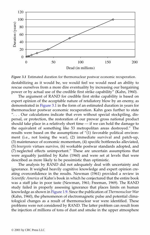
destabilizing as it would be, we would feel we would need an ability torescue ourselves from a more dire eventuality by increasing our bargainingpower or by actual use of the credible first strike capability” (Kahn, 1960).
The argument of RAND for credible first strike capability is based onexpert opinion of the acceptable nature of retaliatory blow by an enemy, asdemonstrated in Figure 3.1 in the form of an estimated duration in years forthermonuclear postwar economic recuperation. Kahn goes further to state“. . . Our calculations indicate that even without special stockpiling, dis-persal, or protection, the restoration of our prewar gross national productshould take place in a relatively short time — if we can hold the damage tothe equivalent of something like 53 metropolitan areas destroyed.” Theresults were based on the assumptions of “(1) favorable political environ-ment (i.e., not losing the war), (2) immediate survival and patch-up,(3) maintenance of economic momentum, (4) specific bottlenecks alleviated,(5) bourgeois virtues survive, (6) workable postwar standards adopted, and(7) neglected effects unimportant.” These are uncertain assumptions thatwere arguably justified by Kahn (1960) and were set at levels that weredescribed as more likely to be pessimistic than optimistic.
The analysis by RAND did not adequately deal with uncertainty andignorance. It weighed heavily cognitive knowledge and expert opinion cre-ating overconfidence in the results. Newman (1961) provided a review inScientific America of Kahn’s book in which he conjectured that the entire bookwas a staff joke in poor taste (Newman, 1961; Freeman, 1969). The RANDstudy failed in properly assessing ignorance that places limits on humanknowledge as shown in Figure 1.9. Since the publication of Thermonuclear War(Kahn, 1960), the phenomenon of electromagnetic pulse and potential clima-tological changes as a result of thermonuclear war were identified. Theseproblems were not considered by RAND. The latter problem can result fromthe injection of millions of tons of dust and smoke in the upper atmosphere
Figure 3.1 Estimated duration for thermonuclear postwar economic recuperation.
0
20
40
60
80
100
120
0 50 100 150
Dead (in millions)
Dur
atio
n (y
ears
)
200
© 2001 by CRC Press LLC

resulting in subfreezing land temperatures for months, and perhaps destroy-ing human food resources such as crops. The effect of 100 to 10,000 totalmegatons of nuclear exchange could conceivably reduce the “population sizeof homosapians to prehistoric levels or below, and the extinction of humanspecies itself cannot be excluded” (Science, 1983). Another failure of the RANDstudy is in logic used to conduct reasoning under uncertainty. For example,Kahn arguably concludes that after a small nuclear destruction scenario of 53metropolitan areas, we will probably restore our gross national product (GNP)quickly. He argues that it is likely that we can handle radiation, it is likely thatwe can handle death, it is likely that we can handle destruction, therefore itis likely that we can handle jointly radiation, death and destruction. As a result,he concludes that we will probably restore our GNP quickly. A fallacy of thislogic in probabilistic reasoning is that high probabilistic likeliness of threepropositions does not necessarily lead to a high probabilistic likeliness of theirjoint proposition. Uncertainty does not propagate in this simple manner aswas used by Kahn. A proper treatment of uncertainty through assessment,modeling, propagation and integration is essential in conjecture.
Example 3.3 NASA’s Challenger space shuttle risk study
NASA sponsored a study to assess the risks associated with the space shuttle(Colglazier and Weatherwax, 1986; Cooke, 1991). In this study, an estimateof solid rocket booster failure probability per launch, based on subjectiveprobabilities and operating experience, was estimated to be about 1 in 35.The probability was based on Bayesian analysis utilizing prior experienceof 32 confirmed failures from 1902 launches of various solid rocket motors.This estimate was disregarded by NASA, and a number of 1 in 100,000 wasdictated based on subjective judgments by managers and administrators(Colglazier and Weatherwax, 1986; Cooke, 1991). The dictated number wasnot in agreement with published data (Bell and Esch, 1989). The catastrophicChallenger explosion occurred on the twenty-fifth launch of a space shuttleon January 28, 1986.
Historically, NASA was distrustful of absolute reliability numbers forvarious reasons. It was publicized that the reliability numbers tend to beoptimistic or taken as facts which they are not (Wiggins, 1985). In reality,failure probabilities can be threatening to the survival of NASA’s missionprograms. For example, a General Electric qualitative probabilistic study onthe probability of successfully landing a man on the moon was 95%. NASAfelt that such numbers could do an irreparable harm, and efforts of this typeshould be disbanded (Bell and Esch, 1989).
At the present, NASA is aggressively pursuing safety studies usingprobabilistic risk analysis of its various space missions. This change inNASA’s practices can be attributed to the extensive investigations followingthe 1986 shuttle disaster.
NASA has used risk assessment matrices to avoid the problem of man-agers treating the values of probability and risk as absolute judgments
© 2001 by CRC Press LLC

(Wiggins, 1985). The Department of Defense offers the use of risk assessmentmatrices as a tool to prioritize risk (Defense Acquisition University, 1998).Qualitatively, the likelihood of occurrence and consequences of an adversescenario may be described as shown in Tables 3.2 and 3.3, respectively.Levels of occurrence may be based on expert-opinion elicitation or actualprobability data. The consequences described in Table 3.3 can be determinedusing expert-opinion elicitation. Tables 3.2 and 3.3 can be combined to fromthe risk matrix. Risk assessment is based on the pairing of the likelihood ofoccurrence and consequences. Table 3.4 shows this pairing and is called arisk assessment matrix.
Table 3.2 Likelihood of Occurrence Level Description Detailed Description
A Frequent Likely to occur frequentlyB Probable Will occur several times in life of a systemC Occasional Likely to occur at sometime in life of a systemD Remote Unlikely but possible to occur in life of a
systemE Improbable So unlikely that it can be assumed its
occurrence may not be experienced
Wiggins, 1985
Table 3.3 ConsequencesLevel Description Mishap Definition
I Catastrophic Death or system lossII Critical Severe injury, severe occupational illness, or
major system damageIII Marginal Minor injury, minor occupational illness, or
minor system damageIV Negligible Less than minor injury, occupational illness,
or system damage
Wiggins, 1985
Table 3.4 Risk Assessment Matrix Using a Risk Index
Likelihood level Consequence levelI
CatastrophicII
CriticalIII
MarginalIV
Negligible
A: Frequent 1 3 7 13B: Probable 2 5 9 16C: Occasional 4 6 11 18D: Remote 8 10 14 19E: Improbable 12 15 17 20
Criteria based onRisk Index:
1-5 = Unacceptable;
6-9 = Undesirable (project management decision required);10-17 = Acceptable with review by project management; and18-20 = Acceptable without review.
Wiggins, 1985
© 2001 by CRC Press LLC
3.3.2 Scenario analysis
The development of scenario analysis can be attributed to Kahn and Wiener(1967). A scenario is defined as a hypothetical sequence of events that areconstructed to focus attention on causal processes and decision points ornodes. Scenario analysis attempts to answer two questions: (1) how mightsome hypothetical situation come about, step by step, and (2) what alterna-tives or choices exist for each actor or party to the situation, at each step, forpreventing, diverting, or facilitating the process. The first question isaddressed in a similar manner to what is called event tree analysis asdescribed by Ayyub and McCuen (1997). The second question is commonlyhandled today using a decision tree as described by Ayyub and McCuen(1997). Kahn and Wiener (1967) used scenario analysis to predict technolog-ical innovations for the year 2000. An examination of their top likely 25technological innovations would reveal a success rate of about 40%. Thepredictions are based on 50% occurrence likelihood.
The scenario analysis by Kahn and Wiener (1967) did not use scenarioprobabilities and relied on identifying what is termed the surprise-free scenariothat is used as a basis for defining alternative futures or canonical variations.The alternative futures or canonical variations are generated by varying keyparameters of the surprise-free scenario. Probabilities, that are absent fromsuch an analysis, are arguably justified by Kahn and Wiener (1967) due tolong-term projections making all scenarios of small likelihood. The surprise-free scenario is considered important due to its ability in defining the long-term trend rather than its likelihood. Therefore, it is important to bear inmind this limitation of scenario analysis, its inability to deliver likelihoodpredictions to us, but only long-term trends. At the present, this limitationcan be alleviated by using event and decision tree analyses.
3.4 Scientific heuristicsThe contemporary philosopher of science Hans Reichenbach (1951) made adistinction between discovery and justification in science. Discovery in sci-ence can be characterized as nonhomogenous, subjective, and nonrational.It can be based on hunches, predictions, biases, and imaginations. It is theproduct of creativity that extends in the domain of the unknown knowledgeto humankind as shown in Figure 1.7. For example, everyone has seen themoon movement across the night sky and seen apples and other objectsfalling to earth; however, it took a Newton to realize the same physical lawsunderlie both phenomena. Newton’s ideas were subjected to testing andvalidation using the scientific processes of justification. There is surely adifference between discovering ideas or phenomena and scientifically justi-fying them. The process of discovery and justification in science can beviewed as a rational consensus process that is based on empirical control(testing) and repeatability; i.e., the outcome of ideas should pass empiricaltesting by anyone and should be repeatable by anyone. Heuristics is a processof discovery that is not necessarily structured.
© 2001 by CRC Press LLC
Discovery is a form of scientific heuristics that does not entail muchstructure and relies heavily on rules of thumb, subjectivity, and creativity.In order to be successful in its pursuit, it cannot approach issues at hand inan orderly fashion but requires a level of coherent disorder that must notreach a level of disarray. Subjectivity and disorder can lead to errors, espe-cially biases, that are not intentional, although intentional or motivationalbiases can be present and should be targeted for elimination. Psychometricresearchers such as Kahneman et al., (1982) and Thys (1987) have studiedthis area extensively on the fundamental level and to understand its relationto expert opinions, respectively.
Heuristics are the product of four factors that could lead to bias:(1) availability, (2) anchoring, (3) representativeness, and (4) control, as shownin Figure 3.2. For a given issue, availability is related to the ease with whichindividuals (including experts) can recall similar events or situations to thisissue. Therefore, probabilities of well-publicized events tend to be overesti-mated, whereas probabilities of unglamorous events are underestimated.
Anchoring is the next factor in heuristics in which subjects, i.e., individ-uals or experts, tend to start with an initial estimate and correct it to theissue at hand. However, the correction might not be sufficient. For example,high school kids guessed the order of magnitude differences in estimatingthe product of the following two number sequences within a short periodof time:
(8 × 7 × 6 × 5 × 4 × 3 × 2 × 1) and (1 × 2 × 3 × 4 × 5 × 6 × 7 × 8)
The differences can be attributed to performing the first few multiplica-tions, establishing anchors, and estimating the final answers through extrap-olation (Kahneman et al., 1982).
Representativeness can affect conditional probability assessments. Forexample, individuals tend to evaluate intuitively the conditional probabilityP(A|B) by assessing the similarity between A and B. The problem with thisassessment is that similarity is symmetric whereas conditional probabilitiesare not; i.e., the resemblance of A to B is the same as the resemblance of Bto A, whereas P(A|B) does not equal P(B|A).
The control factor refers to the perception of subjects in that they cancontrol or had control over outcomes related to an issue at hand. For exam-ple, Langer (1975) demonstrated that lottery ticket buyers demanded highermedian prices for reselling their tickets to a ticket seeker if they had selectedthe ticket numbers than others who were given tickets with randomlyselected numbers. The false sense of control has contributed to a higher beliefin the value of their tickets in comparison to other tickets.
Other sources of bias or error include base-rate fallacy and overconfi-dence. The base-rate fallacy arises as a result of using misguided or misin-formed subjects. A subject might rely on recent or popular information andunintentionally ignore the historic rate for an event of interest. The recent orpopular information might make the subject biased towards a substantially
© 2001 by CRC Press LLC
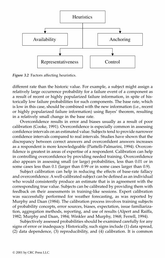
different rate than the historic value. For example, a subject might assign arelatively large occurrence probability for a failure event of a component asa result of recent or highly popularized failure information, in spite of his-torically low failure probabilities for such components. The base rate, whichis low in this case, should be combined with the new information (i.e., recentor highly popularized failure information) using Bayes’ theorem, resultingin a relatively small change in the base rate.
Overconfidence results in error and biases usually as a result of poorcalibration (Cooke, 1991). Overconfidence is especially common in assessingconfidence intervals on an estimated value. Subjects tend to provide narrowerconfidence intervals compared to real intervals. Studies have shown that thediscrepancy between correct answers and overconfident answers increasesas a respondent is more knowledgeable (Piattelli-Palmarini, 1994). Overcon-fidence is greatest in areas of expertise of a respondent. Calibration can helpin controlling overconfidence by providing needed training. Overconfidencealso appears in assessing small (or large) probabilities, less than 0.01 or insome cases less than 0.1 (larger than 0.99 or in some cases larger than 0.9).
Subject calibration can help in reducing the effects of base-rate fallacyand overconfidence. A well-calibrated subject can be defined as an individualwho would consistently produce an estimate that is in agreement with thecorresponding true value. Subjects can be calibrated by providing them withfeedback on their assessments in training-like sessions. Expert calibrationwas successfully performed for weather forecasting, as was reported byMurphy and Daan (1984). The calibration process involves training subjectsof probability concepts, error sources, biases, expectation, issue familiariza-tion, aggregation methods, reporting, and use of results (Alpert and Raiffa,1982; Murphy and Daan, 1984; Winkler and Murphy, 1968; Ferrell, 1994).
Subjectively assessed probabilities should be examined carefully for anysigns of error or inadequacy. Historically, such signs include (1) data spread,(2) data dependence, (3) reproducibility, and (4) calibration. It is common
Figure 3.2 Factors affecting heuristics.
Heuristics
Availability Anchoring
Representativeness Control
© 2001 by CRC Press LLC
to have spread in subjectively assessed probabilities, especially when deal-ing with low numbers (or large numbers for their complementary events).For example, the failure probability per hour of a high-quality steel pipe(10-m long) of a diameter at least 7.6 cm was subjectively assessed by 13experts (Nuclear Regulatory Commission [NCR], 1975) as follows: 5E-6,1E-6, 7E-8, 1E-8, 1E-8, 1E-8, 1E-8, 6E-9, 3E-9, 2E-9, 2E-10, 1E-10, and 1E-10,where 5E-6 mean 5 × 10⁻⁶. The NRC used a value of 1E-10 with 90% confi-dence bounds of 3E-9 and 3E-12 in assessing the annual probability of coremelt due to an earthquake. The following observations can be made basedon these assessments:
1. The data have a spread of 5E-6 to 1E-10 which can be expressed asan upper-limit to lower-limit ratio of about 10,000.
2. The adopted value corresponds to the smallest value in this spread.3. The 90% confidence bounds contain only 5 values out of the 13
gathered values.
Data spread is common in dealing with low numbers. Data spread canbe reduced by asking subjects with extreme views to justify their values, andre-eliciting the data to establish a consensus on a tighter spread, although,it is common to just report and discuss data spread for the purpose ofjustifying and adopting a value with associated confidence bounds.
Data dependence can arise as a result of pessimistic or optimistic sub-jects, i.e., consistently biased subjects that provide low or high values, respec-tively, in comparison to corresponding true (long-term) values. Statisticaltests can be performed on data dependence as a result of using biasedsubjects (Cooke, 1986).
Reproducibility of results can be examined by performing a benchmarkstudy that would require several teams to perform independent analysesbased on a common set of information about a system. Then, the results ofanalyses are compared for spread in the form of ratios of maximum tominimum values reported by the teams. Several benchmark studies of thistype were performed (for example, Amendola, 1986; Brune et al., 1983). TheAmendola (1986) study was structured in four stages using 10 teams fromdifferent European countries to assess the failure probability of a feedwatersystem. The four stages were:
1. The first stage involved blind, independent evaluation by the teamsas an initial probabilistic analysis without information sharingamong the teams. The spread ratio in the resulting probabilities is 25(i.e., 8E-4 and 2E-2).
2. Fault tree analysis was independently performed by the teams re-sulting in a spread ratio of 36. Afterwards the teams met to produceone fault tree, but could not agree on a common one.
3. A common fault tree was assigned to the teams. The teams used theirown data to produce the system failure probability. The spread ratio
© 2001 by CRC Press LLC
in the resulting probabilities is 9. This stage isolates the effect of dataon the results.
4. A common fault tree and data were given to the teams. The teamsused their analytical tools to produce the system failure probability.The spread ratio in the resulting probabilities is about 1. This stageisolates the effect of the analytical tools.
Having data with small spread and without dependence, that have beenreproduced by several teams, does not mean that the data are correct; it onlyincreases our confidence in them. The process of calibration is closely tiedto the process of result validation which is difficult since opinion elicitationis commonly associated with rare events that cannot be validated. Trainingof subjects, however, can be based on other events or issues in order to havecalibrated subjects.
Example 3.4 Information communication for national security intelligence
The intelligence community is in the business of information collection. It isquite common that gathered information is marred with subjectivity, uncer-tainty, and perhaps irrelevance, and it can be from nonreliable sources. Theintelligence community is aware of and regularly deals with these problems.For example, the U.S. Defense Intelligence Agency (DIA) investigated uncer-tainty in intelligence information (Morris and D’Amore, 1980) and provideda summary of various conceptual and analytical models for this purpose.The primary interest of the study was to assess uncertainty in projectingfuture force levels of the former USSR. A secondary motive was to study thefailure to predict the fall of the Shah of Iran in 1979 (Cooke, 1991).
The intelligence community widely used a reliability-accuracy ratingsystem to communicate uncertainty, as shown in Table 3.5. However, Samet(1975) indicated that this system is not adequate, since correspondents tendto emphasize information accuracy, and does not necessarily convey uncer-tainty attributed to source reliability. The DIA used the Kent chart, as shownin Table 3.6, to provide a quantitative interpretation of natural languageexpressions of uncertainty. As reported by Morris and D’Amore (1980), how-ever, the Kent chart has been replaced by a direct use of probabilities.
3.5 Rational consensusThe use of expert opinions in engineering and science needs to be performedas a part of a rational consensus process. A rational consensus process shouldmeet the following requirements (Cooke, 1991):
• Reproducibility. The details of collection, gathering, and computationof results based on expert opinions need to be documents to a level
© 2001 by CRC Press LLC
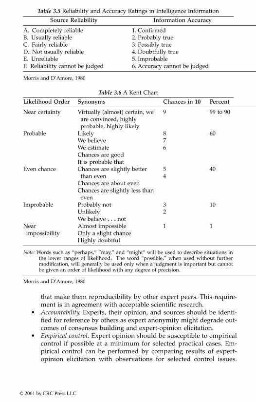
that make them reproducibility by other expert peers. This require-ment is in agreement with acceptable scientific research.
• Accountability. Experts, their opinion, and sources should be identi-fied for reference by others as expert anonymity might degrade out-comes of consensus building and expert-opinion elicitation.
• Empirical control. Expert opinion should be susceptible to empiricalcontrol if possible at a minimum for selected practical cases. Em-pirical control can be performed by comparing results of expert-opinion elicitation with observations for selected control issues.
Table 3.5 Reliability and Accuracy Ratings in Intelligence Information
Source Reliability Information Accuracy
A. Completely reliableB. Usually reliable C. Fairly reliableD. Not usually reliableE. UnreliableF. Reliability cannot be judged
1. Confirmed2. Probably true3. Possibly true4. Doubtfully true5. Improbable6. Accuracy cannot be judged
Morris and D’Amore, 1980
Table 3.6 A Kent Chart
Likelihood Order Synonyms Chances in 10 Percent
Near certainty Virtually (almost) certain, we are convinced, highly probable, highly likely
9 99 to 90
Probable LikelyWe believeWe estimateChances are goodIt is probable that
876
60
Even chance Chances are slightly better than even
Chances are about evenChances are slightly less than even
54
40
Improbable Probably notUnlikelyWe believe . . . not
32
10
Nearimpossibility
Almost impossibleOnly a slight chanceHighly doubtful
1 1
Note: Words such as “perhaps,” “may,” and “might” will be used to describe situations inthe lower ranges of likelihood. The word “possible,” when used without furthermodification, will generally be used only when a judgment is important but cannotbe given an order of likelihood with any degree of precision.
Morris and D’Amore, 1980
© 2001 by CRC Press LLC

This empirical control might not be possible in some situations, butit is in agreement with acceptable scientific research.
• Neutrality. The method of eliciting, evaluating, and combining expertopinions should encourage experts to state their true opinions. Forexample, the use of the median to aggregate expert opinions mightviolate this requirement if the median is perceived to reward centrallycompliant experts. Methods of using weighted averages of opinionsbased on self weights or weights by experts of each other have thesame fallacy.
• Fairness. The experts should be equally treated during the elicitationand for the purposes of processing the observations.
3.6 Elicitation methodsThis section provides a summary of various methods that can be used forelicitation of expert opinions. In order to increase the chances of success inusing elicitation and scoring methods, Cooke (1991) provided suggestedpractices and guidelines. They were revised for the purposes herein, and aresummarized as follows:
1. The issues or questions should be clearly stated without any ambi-guity. Sometimes there might be a need for testing the issues orquestions to ensure their adequate interpretation by others.
2. The questions or issues should be stated using appropriate formatwith listed answers, perhaps graphically expressed, in order to facil-itate and expedite the elicitation and scoring processes.
3. It is advisable to test the processes by performing a dry run.4. The analysts must be present during the elicitation and scoring pro-
cesses.5. Training and calibration of experts must be performed. Examples
should be presented with explanations of elicitation and scoring pro-cesses, and aggregation and reduction of results. The analysts shouldavoid coaching the experts or leading them to certain views andanswers.
6. The elicitation sessions should not be too long. In order to handle manyissues, several sessions with appropriate breaks might be needed.
3.6.1 Indirect elicitation
The indirect elicitation method is popular among theoreticians and wasindependently introduced by Ramsey (1931) and De Finetti (1937). The indi-rect method is based on betting rates by experts in order to reach a point ofindifference among presented options related to an issue. The primary dis-advantage of this method is the utility value of money is not necessarilylinear with the options presented to an expert, and the utility value of moneyis independent of the answer to an issue, such as failure rate.
© 2001 by CRC Press LLC

Other indirect techniques were devised by researchers in order to elicitprobabilities from probability-illiterate experts. For example, analysts haveused time to first failure estimation or age at replacement for a piece ofequipment as an indirect estimation of failure probability.
Example 3.5 Betting rates for elicitation purposes
Betting rates can be used to subjectively and indirectly assess the occurrenceprobability of an event A, called p(A). According to this method, an expertE is hypothetically assigned a lottery ticket of the following form:
Expert E receives $100 if A occurs. (3.1)
The interest hereafter becomes the value that the expert attaches to thislottery ticket. For an assumed amount of money $x, that is less than $100,the expert is asked to trade the ticket for the $x amount. The amount $x isincreased incrementally until a point of indifference is reached; i.e., thelottery ticket has the same value as the offered $x amount. The $x positionis called certainty equivalent to the lottery ticket.
Assuming the expert to be a rational and unbiased agent, the $x positionwhich is certainty equivalent to the lottery ticket, provides an assessment ofan expectation. The expected utility of the lottery ticket can be expressed as
Expected utility of the lottery ticket = $100k(p(A)) (3.2)
where p(A) = the occurrence probability of A, and k = a constant thatrepresent the utility for money as judged by the expert. The utility of moneycan be a nonlinear function of the associated amount. At the certainty equiv-alent position, $x has a utility of k$x, which is equivalent to the expectedutility of the lottery ticket as shown in Equation 3.2. Therefore, the followingcondition can be set:
($100)k(p(A)) = k($x). (3.3)
Solving for p(A) produces
p(A) = . (3.4)
The utility of money in the above example was assumed to be linear,whereas empirical evidence suggests that it is highly nonlinear. Galanter(1962) constructed Table 3.7 by asking subjects the following question:
“Suppose we give you x dollars; reflect on how happyyou are. How much should we have given you in orderto have made you twice as happy?”
$$
x100
© 2001 by CRC Press LLC

The following utility function U was developed based on these data:
U(x) = 3.71x0.43 (3.5)
It is evident that the willingness of people to run a risk does not growlinearly with an increased amount x. Similar tests were performed for lossesof money and their relationship to unhappiness, but were inconclusive assubjects found the questions “too difficult.” Therefore, betting rates mightnot be suitable for failure probability assessment especially since such prob-abilities are commonly very small.
3.6.2 Direct method
This method elicits a direct estimate of the degree of belief of an expert onsome issue. Despite its simple nature, this method might produce the worstresults, especially from experts who are not familiar with the notion of prob-ability. Methods that fall in this category are the Delphi method and thenominal group technique. The Delphi technique, as described in detail inSection 3.3.1, allows for no interaction among the elicited expert before rend-ing opinions. Variations to this method were used by engineers and scientistsby allowing varying levels of interactions that range from limited interactionto complete consensus building. The nominal group technique allows for astructured discussion after the experts have provided initial opinions. Thefinal judgment is made individually on a second cycle of opinion elicitationand aggregated mathematically similar to the Delphi method (Gustafson etal., 1973; Morgan and Henrion, 1992). Lindley (1970) suggested a methodthat is based on comparing an issue to other familiar issues with knownanswers. This comparative examination has been proven to be easier forexperts than directly providing absolute final answers. For example, selectedexperts that are familiar with an event A and its occurrence probability p(A)are accustomed to assessing subjectively the occurrence probability of eventB. We are interested in assessing the occurrence probability of event B thatis not of the same probability familiarity to the experts as p(A). Experts areasked to assess the relative occurrence of B to A, say 10 times as frequent.Therefore, p(B) = 10p(A) as long as the result is less than one.
Table 3.7 Money Required to Double Happiness
Twice as HappyGiven
x Mean Median
$10 $53. $45$20 $538 $350
$1000 $10,220 $5000
Galanter ,1962
© 2001 by CRC Press LLC

3.6.3 Parametric estimation
Parametric estimation is used to assess the confidence intervals on a param-eter of interest such as the mean value. The estimation process can be in theform of a two-step procedure as follows (Preyssl and Cooke, 1989):
1. Obtain a median estimate of a probability (m), and2. Obtain the probability (r) that the true value will exceed 10 times the
median value (m).
The m and r values can be used to compute the 5% and 95% confidencebounds as m/k0.95 and m(k0.95), respectively, where
(3.6)
in which z1–r is the (1–r)th quantile value of the standard normal proba-bility distribution. Some experts were found to like and favor two-stepmethods for dealing with uncertainty.
3.7 Standards for educational and psychological testingCredible behavioral testing and research adhere to the Standards for Educa-tional and Psychological Testing (SEPT) published by the American Psycho-logical Association (1985). The objective of this section is to summarize thesestandards, to determine how they relate to expert-opinion elicitation, and toidentify any pitfalls in expert-opinion elicitation based on examining thesestandards.
Sacman (1975) from the RAND Corporation provided a highly criticalcritique of the Delphi methods based on its lack of compliance with the SEPT,among other scientific and research practices. This critique is valuable andis summarized herein since its applicability in some concerns goes beyondthe Delphi methods to other expert-opinion elicitation methods. Sacman(1975) found that conventional Delphi applications
• often involve crude questionnaire designs,• do not adhere to proper statistical practices of sampling and data
reduction,• do not provide reliability measures,• do not define scope, populations, and limitations,• provide crisply stated answers to ambiguous questions,• involve confusing aggregation methods of expert opinions with sys-
tematic predictions,• inhibit individuality, encourage conformity, and penalize dissidents,• reinforce and institutionalize early closure on issues,
kz r
0 951
0 658.
–
– .≈
( )exp
© 2001 by CRC Press LLC

• can give an exaggerated illusion of precision, and• lack professional accountability.
Although his views are sometimes overstated, they are still useful inhighlighting pitfalls and disadvantages of the Delphi method. The value ofthe Delphi method comes from its initial intended use as a heuristic tool,not a scientific tool, for exploring vague and unknown future issues that areotherwise inaccessible. It is not a substitute for scientific research.
According to the SEPT, a test involves several parties, as follows: testdeveloper, test user, test taker, test sponsor, test administrator, and testreviewer. In expert-opinion elicitation studies, similar parties can be identi-fied. The SEPT provide criteria for the evaluation of tests, testing practices,and the effects of test use. The SEPT provide a frame of reference to supple-ment professional judgment for assessing the appropriateness of a test appli-cation. The standard clauses of the SEPT are classified and identified asprimary standards that should be met by all tests and secondary standards thatare desirable as goals but are likely to be beyond reasonable expectation inmany situations. The SEPT consist of four sections as follows:
Part I. Technical Standards for Test Construction and EvaluationPart II. Professional Standards for Test UsePart III. Standards for Particular ApplicationsPart IV. Standards for Administrative Procedures
These SEPT parts are described in subsequent sections as they relate toexpert-opinion elicitation.
Part I. Technical Standards for Test Construction and EvaluationPart I of the SEPT provides standards for test construction and evaluationthat contain standards for validity, reliability, test development, scaling,norming, comparability, equating, and publication.
The validity consideration of the SEPT covers three aspects: (1) construct-related evidence, (2) content-related evidence, and (3) criterion-related evi-dence. Construct-related evidence primarily focuses on the test score appro-priateness in measuring the psychological characteristic of interest. In theseguidelines, expert-opinion elicitation deals with occurrence likelihood andconsequences. The corresponding test scores can be selected as probabilitiesand consequence units such as dollars. The use of these scores does meetthe validity standards of SEPT in terms of a construct-related evidence. Thecontent-related evidence requires that the selected sample is representativeof some defined universe. In the context of expert-opinion elicitation, expertsshould be carefully selected in order to meet the content-related evidence.The criterion-related evidence needs to demonstrate that the test scores arerelated to a criterion of interest in the real world. In the context of expert-opinion elicitation, the estimated occurrence probabilities and consequencesneed to be related to corresponding real, but unknown, values. This criterion-
© 2001 by CRC Press LLC

related evidence for validity is in agreement with the validation concept inthe AIAA Guide for Verification and Validation of Computational FluidDynamics Simulations, as shown in Figure 3.3. The last consideration invalidity is validity generalization that was reported in the form of the followingtwo uses: (1) to draw scientific conclusions, and (2) to transport the resultvalidity from one case to another. In the context of expert-opinion elicitation,validity generalization based on these two uses might be difficult to justify.Selected primary validity standards, most related to expert-opinion elicita-tion, are shown in Table 3.8. They were taken from the 1997 draft revisionof the SEPT posted on the World Wide Web site of the American Psycholog-ical Association.
The reliability consideration of the SEPT deals with measurement errorsdue to two primary sources: (1) variations from one subject to another thatare subjected to the same conditions and provided with the same backgroundinformation, and (2) variations from one occasion to another by the samesubject. The tools that are needed to estimate the reliability of the scores andtest measurement errors are dependent on the error type. Statistical methodscan be used for this purpose. In the context of expert-opinion elicitation, thisreliability consideration requires aggregation procedures of expert opinionsto include measures of central tendency, biases, dispersion, correlation, vari-ances, standard error of estimates, spread of scores, sample sizes, and pop-ulation definition.
Part I of the SEPT requires that tests and testing programs should bedeveloped on a sound scientific basis. The standards puts the responsibilityon the test developers and publishers to compile evidence bearing on a test,decide which information is needed prior to test publication or distributionand which information can be provided later, and conduct the necessaryresearch.
Figure 3.3 Verification and validation of computational fluid dynamics simulations(AIAA, 1998).
COMPUTERIZED MODEL
REALITY
CONCEPTUAL MODEL
Analysis
Programming
ComputerSimulation
ModelQualification
ModelValidation
ModelVerification
© 2001 by CRC Press LLC
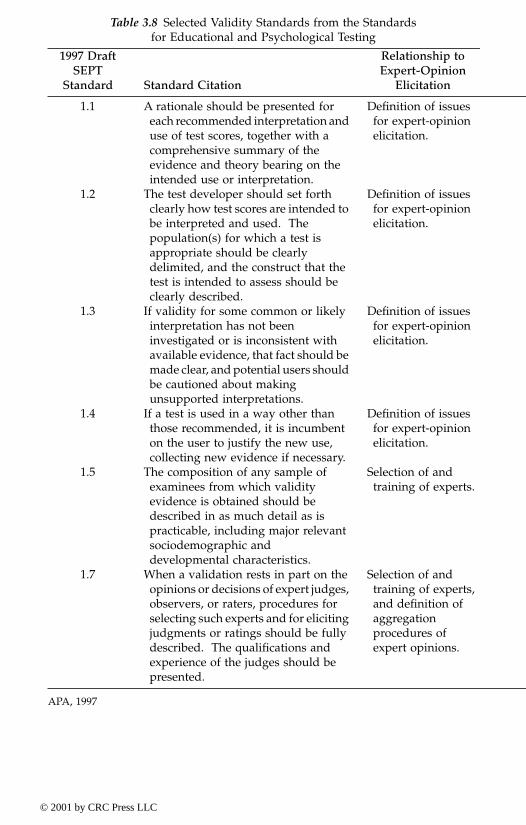
Table 3.8 Selected Validity Standards from the Standardsfor Educational and Psychological Testing
1997 Draft SEPT
Standard Standard Citation
Relationship to Expert-Opinion
Elicitation
1.1 A rationale should be presented for each recommended interpretation and use of test scores, together with a comprehensive summary of the evidence and theory bearing on the intended use or interpretation.
Definition of issues for expert-opinion elicitation.
1.2 The test developer should set forth clearly how test scores are intended to be interpreted and used. The population(s) for which a test is appropriate should be clearly delimited, and the construct that the test is intended to assess should be clearly described.
Definition of issues for expert-opinion elicitation.
1.3 If validity for some common or likely interpretation has not been investigated or is inconsistent with available evidence, that fact should be made clear, and potential users should be cautioned about making unsupported interpretations.
Definition of issues for expert-opinion elicitation.
1.4 If a test is used in a way other than those recommended, it is incumbent on the user to justify the new use, collecting new evidence if necessary.
Definition of issues for expert-opinion elicitation.
1.5 The composition of any sample of examinees from which validity evidence is obtained should be described in as much detail as is practicable, including major relevant sociodemographic and developmental characteristics.
Selection of and training of experts.
1.7 When a validation rests in part on the opinions or decisions of expert judges, observers, or raters, procedures for selecting such experts and for eliciting judgments or ratings should be fully described. The qualifications and experience of the judges should be presented.
Selection of and training of experts, and definition of aggregation procedures of expert opinions.
APA, 1997
© 2001 by CRC Press LLC

The scaling, norming, comparability, and equating considerations in theSEPT deal with aggregation and reduction of scores. The documentation ofexpert-opinion elicitation should provide experts and users with clear expla-nations of the meaning and intended interpretation of derived score scales,as well as their limitations. Measurement scales and aggregation methodswith their limitations, that are used for reporting scores, should be clearlydescribed in expert-opinion elicitation documents. The documents shouldalso include clearly defined populations that are covered by the expert-opinion elicitation process. For studies that involve score equivalence orcomparison and equating of findings, detailed technical information shouldbe provided on equating methods or other linkages and on the accuracy ofequating methods.
Administrators of a test should publish sufficient information on thetests in order for qualified users and reviewers to reproduce the resultsand/or assess the appropriateness and technical adequacy of the test.
Part II. Professional Standards for Test UsePart II of the SEPT provides standards for test use. Users of the results of atest should be aware of methods used in planning, conducting, and reportingthe test in order to appreciate the limitations and scope of use of the test.Documented information on validity and reliability of test results as pro-vided in Part I of the SEPT should be examined by the users for this purpose.
This part also deals with clinical testing, educational and psychologicaltesting at schools, test use in counseling, employment testing, professionaland occupational licensure and certification, and program evaluation. Thesestandards have minimal relevance to expert-opinion elicitation.
Part III. Standards for Particular ApplicationsPart III of the SEPT provides standards for testing linguistic minorities andpeople with handicapping conditions. These standards have minimal rele-vance to expert-opinion elicitation.
Part IV. Standards for Administrative ProceduresPart IV of the SEPT provides standards for test administration, scoring,reporting, and rights of test takers. This part requires that tests should beconducted under standardized and controlled conditions similar to conduct-ing experimental testing. Standardized and controlled conditions enhancethe interpretation of test results by increasing the interpretation quality andeffectiveness. This part also deals with access to test scores, i.e., test securityand cancellation of test scores because of test irregularities.
3.8 Methods of social researchSocial research concerns itself with gathering data on specific questions,issues, or problems of various aspects of society and thus helps humans tounderstand society. Social study has evolved to social science, especially in
© 2001 by CRC Press LLC
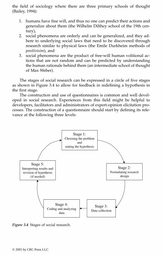
the field of sociology where there are three primary schools of thought(Bailey, 1994):
1. humans have free will, and thus no one can predict their actions andgeneralize about them (the Wilhelm Dilthey school of the 19th cen-tury),
2. social phenomena are orderly and can be generalized, and they ad-here to underlying social laws that need to be discovered throughresearch similar to physical laws (the Emile Durkheim methods ofpositivisim), and
3. social phenomena are the product of free-will human volitional ac-tions that are not random and can be predicted by understandingthe human rationale behind them (an intermediate school of thoughtof Max Weber).
The stages of social research can be expressed in a circle of five stagesas shown in Figure 3.4 to allow for feedback in redefining a hypothesis inthe first stage.
The construction and use of questionnaires is common and well devel-oped in social research. Experiences from this field might be helpful todevelopers, facilitators and administrators of expert-opinion elicitation pro-cesses. The construction of a questionnaire should start by defining its rele-vance at the following three levels:
Figure 3.4 Stages of social research.
Stage 1:Choosing the problem
andstating the hypothesis
Stage 2:Formulating research
design
Stage 3:Data collection
Stage 4:Coding and analyzing
data
Stage 5:Interpreting results andrevision of hypothesis
(if needed)
© 2001 by CRC Press LLC

1. Relevance of the study to the subjects: It is important to communi-cate the goal of the study to the subjects, and establish its relevanceto them. Establishing this relevance would make them stake holdersand thereby increase their attention and sincerity levels.
2. Relevance of the questions to the study: Each question or issue inthe questionnaire needs to support the goal of the study. This ques-tion-to-study relevance is essential to enhancing the reliability ofcollected data from subjects.
3. Relevance of the questions to subjects: Each question or issue inthe questionnaire needs to be relevant to each subject, especiallywhen dealing with subjects of diverse views and backgrounds.
The following are guidelines on constructing questions and statingissues:
• Each item on the questionnaire should include only one question. Itis a poor practice to include two questions in one.
• Question or issue statements should not be ambiguous. Also, the useof ambiguous words should be avoided. In expert-opinion elicitationof failure probabilities, the word “failure” might be vague or ambig-uous to some subjects. Special attention should be given to its defi-nition within the context of each issue or question.
• The level of wording should be kept to a minimum. Long questionsshould be avoided. Also, the word choice might affect the connotationof an issue especially by different subjects. Words should be selectedcarefully to meet the goal of the study in a most reliable manner.
• The use of factual questions is preferred over abstract questions.Questions that refer to concrete and specific matters result in desir-able concrete and specific answers.
• Questions should be carefully structured in order to reduce biases ofsubjects. Questions should be asked in a neutral format, sometimesmore appropriately without lead statements.
• Sensitive topics might require stating questions with lead statementsthat would establish supposedly accepted social norms in order toencourage subjects to answer the questions truthfully.
Questions can be classified as open-ended and closed-ended. A closed-ended question has the following characteristics:
• limits the possible outcomes of response categories,• can provide guidance to subjects thereby making it easier for the
subjects,• provides complete answers,• allows for dealing with sensitive or taboo topics,• allows for comparing the responses of subjects,• produces answers that can be easily coded and analyzed,
© 2001 by CRC Press LLC
• can be misleading,• allows for guesswork by ignorant subjects,• can lead to frustration due to subject perception of inappropriate
answer choices,• limits the possible answer choices,• does not allow for detecting variations in question interpretation by
subjects,• results in artificially small variations in responses due to limiting the
possible answers, and • can be prone to clerical errors by subjects in unintentionally selecting
wrong answer categories.
An open-ended question has the following characteristics:
• does not limit the possible outcomes of response categories,• is suitable for questions without known answer categories,• is suitable for dealing with questions with too many answer catego-
ries,• is preferred for dealing with complex issues,• allows for creativity and self expression,• can lead to collecting worthless and irrelevant information,• can lead to nonstandardized data that cannot be easily compared
among subjects,• can produce data that are difficult to code and analyze,• requires superior writing skills,• might not communicate properly the dimensions and complexity of
the issue,• can be demanding on the time of subjects, and• can be perceived as difficult to answer and thereby discourages sub-
jects from responding accurately or at all.
The format, scale, and units for the response categories should beselected to best achieve the goal of the study. The minimum number ofquestions and question order should be selected with the following guide-lines:
• sensitive questions and open-ended questions should be left to theend of the questionnaire,
• the questionnaire should start with simple questions that are easyto answer,
• a logical order of questions should be developed such that questionsat the start of the questionnaire feed needed information into ques-tions at the end of the questionnaire,
• questions should follow other logical orders that are based on time-sequence or process,
• the order of the questions should not lead or set the response,
© 2001 by CRC Press LLC
• reliability-check questions that are commonly used in pairs (statedpositively and negatively) should be separated by other questions,
• questions should be mixed in terms of format and type in order tomaintain the interest of subjects, and
• the order of the questions can establish a funnel by starting withgeneral questions followed by more specific questions within severalbranches of questioning; this funnel technique might not be appro-priate in some applications, and its suitability should be assessed ona case-by-case basis.
The final stage of developing a questionnaire is writing a cover letter orintroductory statement, instructions to interviewers, subjects, or facilitators,precoding, and pretesting. The introductory statement should provide thegoal of the study and establish relevance. The instructions should provideguidance on expectations, completion of questionnaire, and reporting. Pre-coding assigns numerical values to responses for the purpose of data analysisand reduction. Pretesting should be administered to a few subjects for thepurpose of identifying and correcting flaws.
Some of the difficulties or pitfalls of using questionnaires, with suggestedsolutions or remedies, include the following (Bailey, 1994):
1. Subjects might feel that the questionnaire is not legitimate and has ahidden agenda. A cover letter or a proper introduction of the ques-tionnaire is needed.
2. Subjects might feel that the results will be used against them. Unnec-essary sensitive issues and duplicate issues should be removed.Sometimes assuring a subject’s anonymity might provide the neededremedy.
3. Subjects might refuse to answer questions on the basis that they havedone their share of questionnaires or are tired of “being a guineapig.” Training and education might be needed to create the properattitude.
4. A “sophisticated” subject who participated in many studies mayhave thereby developed an attitude of questioning the structure ofthe questionnaire, test performance, and result use and might requirea “sampling around” to find a replacement subject.
5. A subject might provide “normative” answers, i.e., answers that thesubject thinks are being sought. Unnecessarily sensitive issues andduplicate issues should be removed. Sometimes assuring a subject’sanonymity might provide the needed remedy.
6. Subjects might not want to reveal their ignorance and perhaps appearstupid. Emphasizing that there are no correct or wrong answers, andassuring a subject’s anonymity, might provide the needed remedy.
7. A subject might think that the questionnaire is a waste of time.Training and education might be needed to create the proper attitude.
8. Subjects might feel that a question is too vague and cannot be an-swered. The question should be restated so that it is very clear.
© 2001 by CRC Press LLC
3.9 Focus groupsThe concept of focus groups was started in the 1930s when social scientistsbegan questioning the appropriateness and accuracy of information thatresulted from individual subject interviews using questionnaires withclosed-ended response choices; they began investigating alternative waysfor conducting interviews. Rice (1931) expressed his concern of having aquestioner taking the lead, with subjects taking a more or less passive role;thereby resulting in not capturing information of the highest value as a resultof the questioner’s, intentionally or unintentionally, leading the subjectsaway. As a result, information gathered at interviews might embody precon-ceived ideas of the questioner as well as the attitude of the subjects inter-viewed. During World War II, social scientists started using nondirectiveinterview techniques in groups as a start of focus groups. The first use offocus groups was by the War Department to assess morale of the U.S. mili-tary. It was noted that people tend to reveal sensitive information once theyare in a safe, comfortable environment with people like themselves, asdescribed in the classic book on focus groups by Merton, et al. (1956).
Focus groups are commonly used in assessing markets, product devel-opments, developing price strategies for new products and their variations,and assessing some issues of interest. A focus group can be defined as aspecial type of group, in terms of purpose, size, composition, and procedures,that has a purpose of listening and gathering information based on howpeople feel or think about an issue (Krueger and Casey, 2000). The intent offocus groups is to promote self-disclosure among the subjects by revealingwhat people really think and feel.
Focus groups are popular in terms of use by commercial business,foundations, governmental agencies, and schools. The size of the group canbe approximately six to twelve subjects, depending on the application andissues considered. For market research, the subjects should not know eachother, preferably being strangers, but it is not an issue in other types ofresearch. Each focus group should have a professional or qualified moder-ator. The focus groups should be held in special rooms with one-waymirrors and quality acoustics for market research, but they can be held inregular meeting rooms or a lounge for other applications. A list of questionsshould be prepared that generally can be structured as (1) opening ques-tions, (2) introductory questions, (3) transition questions, (4) key questions,(5) ending questions. The questions should be structured and stated so thatthey are engaging to participants. The questions should be developed bya group of analysts through brainstorming, phrasing of questions, sequenc-ing the questions, estimating time needed for questions, getting feedbackfrom others, and testing the questions. The data can be captured throughobservation behind mirrors, audio and video recording, and/or field notes.The results can be analyzed in various manners depending on the issue orapplication. The analysis methods can range from rapid first impression bya moderator or an analyst, to transcripts followed by rigorous analysis using
© 2001 by CRC Press LLC

analytical and statistical methods, to abridged transcripts with charts andaudiotapes. A report should be prepared documenting the process andresults. The report should then be sent to the sponsor (in the case of marketresearch), can be provided to public officials, can be shared with the par-ticipants, or can be shared with a community. The time needed to completea focus group study is about two weeks in the case of market research toseveral months in other applications.
Krueger and Casey (2000) provide variations and tips to the above gen-eral model for convening and using focus groups for special cases, such asdealing with existing organizations, young people, ethnic or minoritygroups, international groups or organizations, periodically repeated groups,telephone and Internet focus groups, and media focus groups.
3.10 Exercise problemsProblem 3.1 What are the primary pitfalls of using the Delphi method?Provide examples.
Problem 3.2 What are the advantages of using the Delphi method? Whenwould you use a Delphi type of a method? Provide examples.
Problem 3.3 What are the differences between the Delphi method and sce-nario analysis? Provide examples to demonstrate the differences. Can youprovide an example in which both the Delphi method and scenario analysisshould be used?
Problem 3.4 What are the factors that could bias scientific heuristics results?Provide examples.
Problem 3.5 What is the base-rate fallacy? How can it lead to an opinion inerror?
Problem 3.6 Using the method of parametric estimation, compute the 5%and 95% confidence bounds on a concrete strength parameter based on amedian (m) of 3000 ksi and the probability (r) of 0.01.
Problem 3.7 Using the method of parametric estimation, compute the 5%and 95% confidence bounds on a parameter based on a median (m) of 100and the probability (r) of 0.02.
Problem 3.8 Construct a questionnaire that meets the Standards for Educa-tional and Psychological Testing (SEPT) and social research to determine themeaning of unethical conduct in exam taking by students, and of studentpreferences, and probabilities of cheating, when taking in-class and take-home exams.
Problem 3.9 Construct a questionnaire that meets the SEPT and socialresearch to determine the meaning of unethical conduct in engineering work-places by engineers and probabilities of its occurrence.
Problem 3.10 What are the differences between a focus group and a Delphisession?
© 2001 by CRC Press LLC

chapter four
Expressing and modeling expert opinions
Contents
4.1. Introduction4.2. Set theory
4.2.1. Sets and events4.2.2. Fundamentals of classical set theory
4.2.2.1. Classifications of sets4.2.2.2. Subsets4.2.2.3. Membership (or characteristic) function4.2.2.4. Sample space and events4.2.2.5. Venn-Euler diagrams4.2.2.6. Basic operations on sets
4.2.3. Fundamentals of fuzzy sets and operations4.2.3.1. Membership (or characteristic) function4.2.3.2. Alpha-cut sets4.2.3.3. Fuzzy Venn-Euler diagrams4.2.3.4. Fuzzy numbers, intervals, and arithmetic4.2.3.5. Operations on fuzzy sets4.2.3.6. Fuzzy relations4.2.3.7. Fuzzy functions
4.2.4. Fundamental of rough sets4.2.4.1. Rough set definitions4.2.4.2. Rough set operations4.2.4.3. Rough membership functions4.2.4.4. Rough functions
4.3. Monotone measures4.3.1. Definition of monotone measures4.3.2. Classifying monotone measures
© 2001 by CRC Press LLC
4.3.3. Evidence theory4.3.3.1. Belief measure4.3.3.2. Plausibility measure4.3.3.3. Basic assignment
4.3.4. Probability theory4.3.4.1. Relationship between evidence theory
and probability theory4.3.4.2. Classical definitions of probability4.3.4.3. Linguistic probabilities4.3.4.4. Failure rates4.3.4.5. Central tendency measures4.3.4.6. Dispersion (or variability)4.3.4.7. Percentiles4.3.4.8. Statistical uncertainty4.3.4.9. Bayesian methods4.3.4.10. Interval probabilities4.3.4.11. Interval cumulative distribution functions4.3.4.12. Probability bounds
4.3.5. Possibility theory4.4. Exercise problems
4.1 IntroductionWe seek experts for their opinions on issues identified as of interest to us.Appropriate definitions of these issues and formats for anticipated judg-ments are critical for the success of an expert-opinion elicitation process.This chapter provides background information and analytical tools that canbe used to express expert opinions and model these opinions. The expressionof a view or judgment by an expert is an important link in the success ofthe process. The expression of an opinion can be defined as putting it intowords or numbers, or representing the opinion in language, a picture, or afigure. The manner of expressing the opinion in a meaningful and eloquentmanner is an important characteristic. The expression might be sensitive tothe choice of a particular word, phrase, sentence, symbol, or picture. It canalso include a show of feeling or character. It can be in the form of a symbolor set of symbols expressing some mathematical or analytical relationship,as a quantity or operation.
In this chapter, we present the fundamentals of classical set theory, fuzzysets, and rough sets that can be used to express opinions. Basic operationsfor these sets are defined and demonstrated. Fuzzy relations and fuzzyarithmetic can be used to express and combine collected information. Thefundamentals of probability theory, possibility theory, interval probabilities,and monotone measures will be summarized as they relate to the expressionof expert opinions. Examples are used in this chapter to demonstrate thevarious methods and concepts.
© 2001 by CRC Press LLC
4.2 Set theory4.2.1 Sets and events
Sets constitute a fundamental concept in probabilistic analysis of engineeringproblems. Informally, a set can be defined as a collection of elements orcomponents. Capital letters are usually used to denote sets, e.g., A, B, X, Y,. . ., etc. Small letters are commonly used to denote their elements, e.g., a, b,x, y, . . ., etc., respectively.
4.2.2 Fundamentals of classical set theory
The fundamental difference between classical (crisp or nonfuzzy) sets andfuzzy sets is that belonging and nonbelonging to sets are assumed to bewithout any form of uncertainty in the former and with uncertainty in thelatter. This assumption that elements belong or do not belong to sets withoutany uncertainty constitutes a basis for the classical set theory. If this assump-tion is relaxed to allow some form of uncertainty in belonging or nonbelong-ing to sets, then the notion of fuzzy sets can be introduced where belongingand nonbelonging involve variable levels of uncertainty.
Example 4.1 Selected crisp sets
The following are example sets:
A = {2, 4, 6, 8, 10} (4.1)
B = {b: b > 0 }; where “:” means “such that” (4.2)
C = {Maryland, Virginia, Washington} (4.3)
D = {P, M, 2, 7, U, E} (4.4)
F = {1, 2, 3, 4, 5, 6, 7, . . .}; the set of odd numbers (4.5)
In these example sets, each set consists of a collection of elements. In setA, 2 belongs to A, and 12 does not belong to A. Using mathematical notations,this can be expressed as 2 ∈ A, and 12 ∉ A, respectively.
4.2.2.1 Classifications of setsSets can be classified as finite and infinite sets. For example, sets A, C, and Din Example 4.1 are finite sets, whereas sets B and F are infinite sets. Theelements of a set can be either discrete or continuous. For example, the ele-ments of sets A, C, D, and F are discrete, whereas the elements in set B arecontinuous. A set without any elements is named the null (or empty) set Ø.
© 2001 by CRC Press LLC
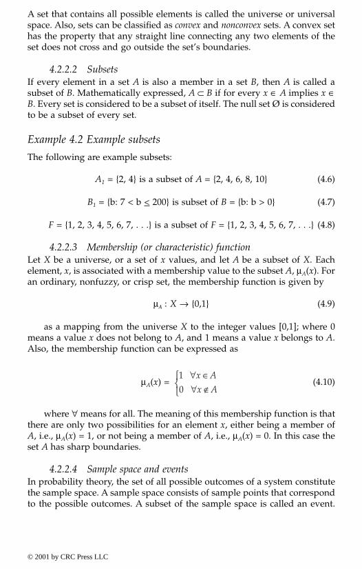
A set that contains all possible elements is called the universe or universalspace. Also, sets can be classified as convex and nonconvex sets. A convex sethas the property that any straight line connecting any two elements of theset does not cross and go outside the set’s boundaries.
4.2.2.2 SubsetsIf every element in a set A is also a member in a set B, then A is called asubset of B. Mathematically expressed, A ⊂ B if for every x ∈ A implies x ∈B. Every set is considered to be a subset of itself. The null set Ø is consideredto be a subset of every set.
Example 4.2 Example subsets
The following are example subsets:
A1 = {2, 4} is a subset of A = {2, 4, 6, 8, 10} (4.6)
B1 = {b: 7 < b < 200} is subset of B = {b: b > 0} (4.7)
F = {1, 2, 3, 4, 5, 6, 7, . . .} is a subset of F = {1, 2, 3, 4, 5, 6, 7, . . .} (4.8)
4.2.2.3 Membership (or characteristic) functionLet X be a universe, or a set of x values, and let A be a subset of X. Eachelement, x, is associated with a membership value to the subset A, µA(x). Foran ordinary, nonfuzzy, or crisp set, the membership function is given by
µA : X → {0,1} (4.9)
as a mapping from the universe X to the integer values [0,1]; where 0means a value x does not belong to A, and 1 means a value x belongs to A.Also, the membership function can be expressed as
µA(x) = (4.10)
where ∀ means for all. The meaning of this membership function is thatthere are only two possibilities for an element x, either being a member ofA, i.e., µA(x) = 1, or not being a member of A, i.e., µA(x) = 0. In this case theset A has sharp boundaries.
4.2.2.4 Sample space and eventsIn probability theory, the set of all possible outcomes of a system constitutethe sample space. A sample space consists of sample points that correspondto the possible outcomes. A subset of the sample space is called an event.
10
∀ ∈∀ ∉
x A
x A
© 2001 by CRC Press LLC
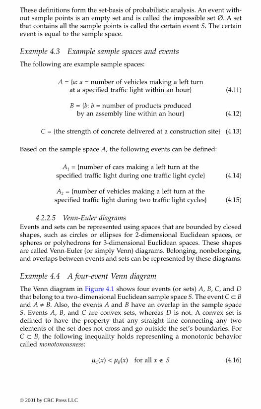
These definitions form the set-basis of probabilistic analysis. An event with-out sample points is an empty set and is called the impossible set Ø. A setthat contains all the sample points is called the certain event S. The certainevent is equal to the sample space.
Example 4.3 Example sample spaces and events
The following are example sample spaces:
A = {a: a = number of vehicles making a left turnat a specified traffic light within an hour} (4.11)
B = {b: b = number of products producedby an assembly line within an hour} (4.12)
C = {the strength of concrete delivered at a construction site} (4.13)
Based on the sample space A, the following events can be defined:
A1 = {number of cars making a left turn at thespecified traffic light during one traffic light cycle} (4.14)
A2 = {number of vehicles making a left turn at thespecified traffic light during two traffic light cycles} (4.15)
4.2.2.5 Venn-Euler diagramsEvents and sets can be represented using spaces that are bounded by closedshapes, such as circles or ellipses for 2-dimensional Euclidean spaces, orspheres or polyhedrons for 3-dimensional Euclidean spaces. These shapesare called Venn-Euler (or simply Venn) diagrams. Belonging, nonbelonging,and overlaps between events and sets can be represented by these diagrams.
Example 4.4 A four-event Venn diagram
The Venn diagram in Figure 4.1 shows four events (or sets) A, B, C, and Dthat belong to a two-dimensional Euclidean sample space S. The event C ⊂ Band A ≠ B. Also, the events A and B have an overlap in the sample spaceS. Events A, B, and C are convex sets, whereas D is not. A convex set isdefined to have the property that any straight line connecting any twoelements of the set does not cross and go outside the set’s boundaries. ForC ⊂ B, the following inequality holds representing a monotonic behaviorcalled monotonousness:
µC(x) < µB(x) for all x ∉ S (4.16)
© 2001 by CRC Press LLC
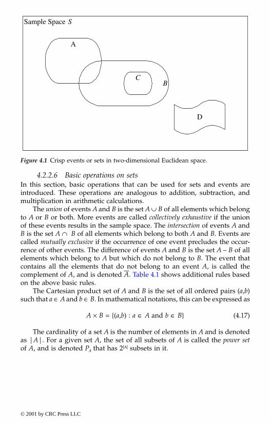
4.2.2.6 Basic operations on setsIn this section, basic operations that can be used for sets and events areintroduced. These operations are analogous to addition, subtraction, andmultiplication in arithmetic calculations.
The union of events A and B is the set A ∪ B of all elements which belongto A or B or both. More events are called collectively exhaustive if the unionof these events results in the sample space. The intersection of events A andB is the set A ∩ B of all elements which belong to both A and B. Events arecalled mutually exclusive if the occurrence of one event precludes the occur-rence of other events. The difference of events A and B is the set A – B of allelements which belong to A but which do not belong to B. The event thatcontains all the elements that do not belong to an event A, is called thecomplement of A, and is denoted A. Table 4.1 shows additional rules basedon the above basic rules.
The Cartesian product set of A and B is the set of all ordered pairs (a,b)such that a ∈ A and b ∈ B. In mathematical notations, this can be expressed as
A × B = {(a,b) : a ∈ A and b ∈ B} (4.17)
The cardinality of a set A is the number of elements in A and is denotedas |A|. For a given set A, the set of all subsets of A is called the power setof A, and is denoted PA that has 2|A| subsets in it.
Figure 4.1 Crisp events or sets in two-dimensional Euclidean space.
Sample Space S
A
BC
D
© 2001 by CRC Press LLC
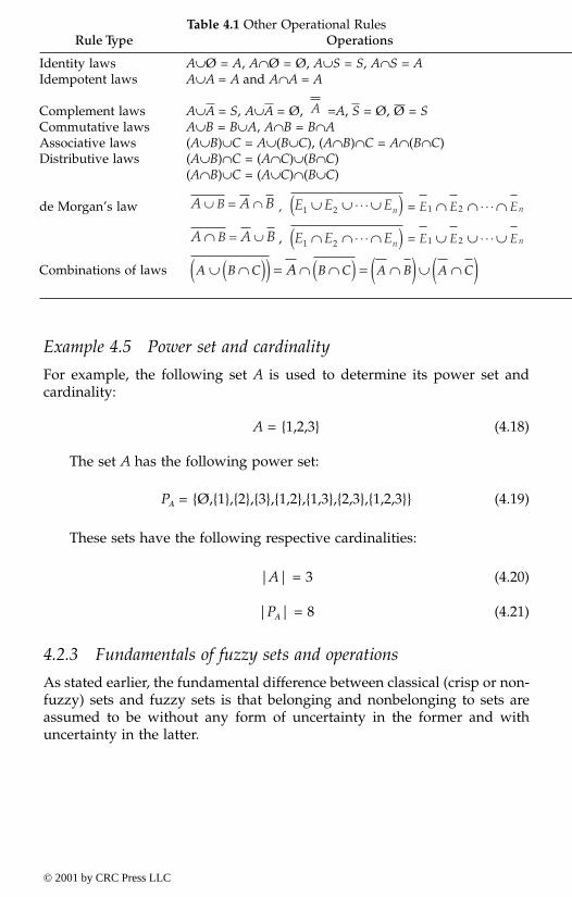
Example 4.5 Power set and cardinality
For example, the following set A is used to determine its power set andcardinality:
A = {1,2,3} (4.18)
The set A has the following power set:
PA = {Ø,{1},{2},{3},{1,2},{1,3},{2,3},{1,2,3}} (4.19)
These sets have the following respective cardinalities:
|A| = 3 (4.20)
|PA| = 8 (4.21)
4.2.3 Fundamentals of fuzzy sets and operations
As stated earlier, the fundamental difference between classical (crisp or non-fuzzy) sets and fuzzy sets is that belonging and nonbelonging to sets areassumed to be without any form of uncertainty in the former and withuncertainty in the latter.
Table 4.1 Other Operational RulesRule Type Operations
Identity laws A∪Ø = A, A∩Ø = Ø, A∪S = S, A∩S = AIdempotent laws A∪A = A and A∩A = A
Complement laws A∪A = S, A∪A = Ø, = A, S = Ø, Ø = SCommutative laws A∪B = B∪A, A∩B = B∩AAssociative laws (A∪B)∪C = A∪(B∪C), (A∩B)∩C = A∩(B∩C)Distributive laws (A∪B)∩C = (A∩C)∪(B∩C)
(A∩B)∪C = (A∪C)∩(B∪C)
de Morgan’s law , =
, =
Combinations of laws
A
A A BB∪ = ∩ E E En1 2∪ ∪ ⋅⋅ ⋅ ∪( ) E E E n1 2∩ ∩ ⋅⋅ ⋅ ∩
A A BB∩ = ∪ E E En1 2∩ ∩ ⋅⋅ ⋅ ∩( ) E E E n1 2∪ ∪ ⋅⋅ ⋅ ∪
A B C B C A B A CA∪ ∩( )( ) = ∩ ∩( ) = ∩( ) ∪ ∩( )
© 2001 by CRC Press LLC
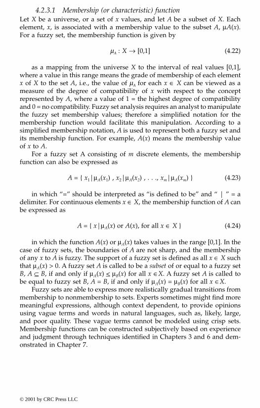
4.2.3.1 Membership (or characteristic) functionLet X be a universe, or a set of x values, and let A be a subset of X. Eachelement, x, is associated with a membership value to the subset A, µA(x).For a fuzzy set, the membership function is given by
µA : X → [0,1] (4.22)
as a mapping from the universe X to the interval of real values [0,1],where a value in this range means the grade of membership of each elementx of X to the set A, i.e., the value of µA for each x ∈ X can be viewed as ameasure of the degree of compatibility of x with respect to the conceptrepresented by A, where a value of 1 = the highest degree of compatibilityand 0 = no compatibility. Fuzzy set analysis requires an analyst to manipulatethe fuzzy set membership values; therefore a simplified notation for themembership function would facilitate this manipulation. According to asimplified membership notation, A is used to represent both a fuzzy set andits membership function. For example, A(x) means the membership valueof x to A.
For a fuzzy set A consisting of m discrete elements, the membershipfunction can also be expressed as
A = { x1|µA(x1) , x2|µA(x2) , . . ., xm|µA(xm) } (4.23)
in which “=” should be interpreted as “is defined to be” and “ | ” = adelimiter. For continuous elements x ∈ X, the membership function of A canbe expressed as
A = { x|µA(x) or A(x), for all x ∈ X } (4.24)
in which the function A(x) or µA(x) takes values in the range [0,1]. In thecase of fuzzy sets, the boundaries of A are not sharp, and the membershipof any x to A is fuzzy. The support of a fuzzy set is defined as all x ∈ X suchthat µA(x) > 0. A fuzzy set A is called to be a subset of or equal to a fuzzy setB, A ⊆ B, if and only if µA(x) < µB(x) for all x ∈X. A fuzzy set A is called tobe equal to fuzzy set B, A = B, if and only if µA(x) = µB(x) for all x ∈X.
Fuzzy sets are able to express more realistically gradual transitions frommembership to nonmembership to sets. Experts sometimes might find moremeaningful expressions, although context dependent, to provide opinionsusing vague terms and words in natural languages, such as, likely, large,and poor quality. These vague terms cannot be modeled using crisp sets.Membership functions can be constructed subjectively based on experienceand judgment through techniques identified in Chapters 3 and 6 and dem-onstrated in Chapter 7.
© 2001 by CRC Press LLC

Example 4.6 Fuzzy sets to represent experience
As an example of fuzzy sets, let X be the experience universe of an individualto perform some job, such that x ∈ X can take a real value in the range fromx = 0 meaning absolutely no experience in performing the job to x = 100 meaningabsolutely the highest level of experience. The range 0 to 100 was selected forrepresentation convenience. Other ranges could be used such as 0 to 1. Fivelevels of experience are shown in Figure 4.2 using linguistic descriptors, suchas low, medium, and high experience. These experience classification aremeaningful although vague. A fuzzy set representation offers a means oftranslating this vagueness into meaningful numeric expressions using mem-bership functions.
Another method of presenting fuzzy sets that was used in the 1980s isbased on dividing the range of experience into increments of 10. Therefore,a linguistic variable of the type “low or short experience,” designated as A,can be expressed using the following illustrative fuzzy definition that doesnot correspond to Figure 4.2:
short experience, A = { x1 = 100 | µA(x1) = 0 , x2 = 90 | µA(x2) = 0,
x3 = 80 | µA(x3) = 0 , x4 = 70 | µA(x4) = 0 , x5 = 60 | µA(x5) = 0,
x6 = 50 | µA(x6) = 0 , x7 = 40 | µA(x7) = 0.1 , x8 = 30 | µA(x8) = 0.5,
x9 = 20 | µA(x9) = 0.7 , x10 = 10 | µA(x10) = 0.9 , x11 = 0 | µA(x11) = 1.0 } (4.25)
Figure 4.2 Experience levels as fuzzy sets.
Experience0 100
Mem
bers
hip
Val
ue
1
0
Low Medium HighLow-Medium Medium-High
© 2001 by CRC Press LLC

This expression can be written in an abbreviated form by showing expe-rience levels with only non-zero membership values as follows:
short experience, A ={ 40|0.1, 30|0.5, 20|0.7, 10|0.9, 0|1.0 } (4.26)
The fuzziness in the definition of short experience is obvious from Equa-tions 4.25 or 4.26 as opposed to a definition in the form of Equation 4.9.Based on the fuzzy definition of short experience, different grades of expe-rience have different membership values to the fuzzy set, “short experienceA.” The membership values are decreasing as a function of increasing gradeof experience. In this example, the values of x with nonzero membershipvalues are 40, 30, 20, 10, and 0, and the corresponding membership valuesare 0.1, 0.5, 0.7, 0.9, and 1.0, respectively. Other values of x larger than 40have zero membership values to the subset A. These membership valuesshould be assigned based on subjective judgment with the help of expertsand can be updated with more utilization of such linguistic measures in reallife applications. If a crisp set were used in this example of defining shortexperience, the value of x would be 0 with a membership value of 1.0.Similarly, long experience, B, can be defined as
long experience, B ={ 100|1, 90|0.9, 80|0.7, 70|0.2, 60|0.1 } (4.27)
It should be noted that Equations 4.25 – 4.27 show experience takingdiscrete values for convenience only since values between these discretevalues have membership values that can be computed using interpolationbetween adjacent values. In order to use fuzzy sets in practical problems,some operational rules similar to those used in classical set theory (Table4.1) need to be defined.
4.2.3.2 Alpha-cut setsFuzzy sets can be described effectively and in a manner that can facilitatethe performance of fuzzy-set operations using an important concept of anα-cut. For a fuzzy set A defined on universe X and a number α in the unitinterval of membership [0, 1], the α-cut of A, denoted by αA, is the crisp setthat consists all elements of A with membership degrees in A greater thanor equal to α. An α-cut of A as a crisp set can be expressed as
αA = {x: A(x) ≥ α} (4.28)
which means the crisp sets of x values such that A(x) is greater or equalto α. For fuzzy sets of continuous real values and membership functionswith one mode, i.e., unimodal functions, the resulting α-cut of A is an intervalof real values. Such fuzzy sets and membership functions are common inengineering and sciences. A strong α-cut of A is defined as
© 2001 by CRC Press LLC

α+A = {x: A(x) > α} (4.29)
The α-cut of A, with α = 1.0, is called the core set of the fuzzy set A. Afuzzy set with an empty core set is called a subnormal fuzzy set since thelargest value of its membership function is less than one; otherwise the fuzzyset is called a normal set.
A set of nested αA can be constructed by incrementally changing thevalue of α. A convenient representation of such nested sets at quartile αvalues is as follows:
Nested αA = {(αi, xLi, xRi)} for i = 1,2,3,4,5 (4.30)
where the five sets of triplets correspond to α values of 1, 0.75, 0.50, 0.25,and 0+, respectively, and L and R refer to left and right, respectively. Theα–cut of A, with α+ = 0+, is called the support set of the fuzzy set A. Otherquartile levels can be termed upper quartile set, mid quartile set, and lowerquartile set.
Example 4.7 α-cut of experience
Figure 4.3 shows a fuzzy-set representation or expression of medium expe-rience based on the subjective assessment of an expert. The fuzzy set has acore set defined by the real range [40,60], and a support defined by [20,80].The α-cuts of A are shown in Table 4.2 for all the quartile values and can beexpressed as:
Nested αA for Medium Experience = {(1,40,60), (0.75,35,65), (0.5,30,70), (0.25,25,75), (0+,20,80)} (4.31)
4.2.3.3 Fuzzy Venn-Euler diagramsSimilar to crisp events, fuzzy events and sets can be represented using spacesthat are bounded by closed shapes, such as circles with fuzzy boundariesshowing the transitional stage from membership to nonmembership. Belong-ing, nonbelonging, and overlaps between events and sets can be representedby these diagrams. Figure 4.4 shows an example fuzzy event (or set) A withfuzzy boundaries. The various nested shapes can be considered similar tocontours in topographical representations that correspond to the five-quar-tile α-cuts of A.
Table 4.2 α-cuts of Medium Experience as Provided in Figure 4.3
αααα Left limit (xL) Right limit (xR) Name of set
1. 40 60 Core set0.75 35 65 Upper quartile set0.50 30 70 Mid quartile set0.25 25 75 Lower quartile set0. 20 80 Support set
© 2001 by CRC Press LLC
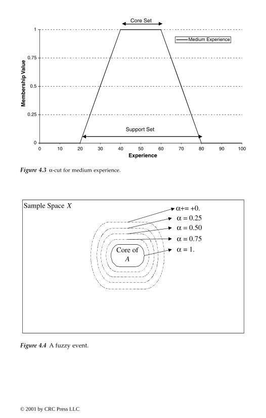
Figure 4.3 α-cut for medium experience.
Figure 4.4 A fuzzy event.
0
0.25
0.5
0.75
1
0 10 20 30 40 50 60 70 80 90 100
Experience
Mem
ber
ship
Val
ue
Medium Experience
Core Set
Support Set
Sample Space X
Core ofA
α+= +0. α = 0.25 α = 0.50
α = 0.75
α = 1.
© 2001 by CRC Press LLC

4.2.3.4 Fuzzy numbers, intervals and arithmeticA fuzzy number is defined as an approximate numerical value whose bound-ary is not sharp and can be characterized by a membership grade function.The membership function µA(x) for a fuzzy number A can be defined as givenin Equation 4.22. An α-cut of a fuzzy number A can also be defined asprovided by Equation 4.28. If the shape of the membership function istriangular, the fuzzy set is called a triangular fuzzy number. An α-cut of afuzzy number (or set) A can be expressed as either by the five quartiles ofEquation 4.30 or for an individual α as
αA = [xL, xR] = [aL, aR] (4.32)
where L and R are the left and right x limits of the interval at α. Atriangular fuzzy number A can be denoted as A[a, am, b], where a = the lowestvalue of support, b = highest value of support, and am = is the middle valueat the mode of the triangle. A trapezoidal fuzzy interval A can similarly bedenoted as A[a, amL, amR, b], where a = the lowest value of support, b = highestvalue of support, and amL and amR = are the left and right middle values atthe mode range of the trapezoid. A triangular fuzzy number is commonlyused to represent an approximate number, such as, the weight of a machineis approximately 200 pounds; whereas a trapezoidal fuzzy interval is anapproximate interval, such as, the capacity of a machine is approximately200 to 250 pounds. These examples of fuzzy numbers and fuzzy intervalsare shown in Figure 4.5 with their crisp counterparts, where a crisp numbercan be represented as
A = am (4.33)
A fuzzy number A[a, am, b] can be represented as
(4.34)
A crisp interval can be represented as
A = [am1,am2] (4.35)
A x
x a
a aa x a
x b
a ba x b
mm
mm( ) =
≤ ≤
≤ ≤
–
–
–
–
for
for
otherwise0
© 2001 by CRC Press LLC

Figure 4.5a Crisp number.
Figure 4.5b Fuzzy numbers.
0
0.25
0.5
0.75
1
160 170 180 190 200 210 220 230 240
Weight
Mem
ber
ship
Val
ue
a) Exactly 200 pounds
0
0.25
0.5
0.75
1
160 170 180 190 200 210 220 230 240
Weight
Mem
ber
ship
Val
ue
b) Approximately 200 pounds
© 2001 by CRC Press LLC

Figure 4.5c Crisp interval.
Figure 4.5d Fuzzy interval.
0
0.25
0.5
0.75
1
160 170 180 190 200 210 220 230 240 250 260 270 280 290
Capacity
Mem
ber
ship
Val
ue
c) Exactly 200 to 250 pounds
0
0.25
0.5
0.75
1
160 170 180 190 200 210 220 230 240 250 260 270 280 290
Capacity
Mem
ber
ship
Val
ue
d) Approximately 200 to 250 pounds
© 2001 by CRC Press LLC

A fuzzy interval A[a, amL, amR, b] can be represented as
(4.36)
For two fuzzy numbers or intervals A and B, let αA = [aL, aR]and αB =[bL, bR], where a and b are real numbers on the left (L) and right (R) ends ofthe ranges, and α ∈ [0,1] The fuzzy arithmetic of addition, subtraction,multiplication, and division, respectively, can be defined as follows (Kauf-mann and Gupta, 1985) based on interval-valued arithmetic (Moore, 1966and 1979):
αA + αB = [aL, aR] + [bL, bR] = [aL + bL, aR + bR] (4.37)
αA – αB = [aL, aR] – [bL, bR] = [aL – bR, aR – bL] (4.38)
αA × αB = [aL, aR] × [bL, bR] = [min (aL bL, aL bR, aR bL, aR bR), (4.39)max(aL bL, aL bR, aR bL, aR bR)]
αA / αB = [aL, aR] / [bL, bR] = [min (aL/bL, aL/bR, aR/bL, aR/bR), (4.40)max(aL/bL, aL/bR, aR/bL, aR/bR)]
Equation 4.40 requires that 0 ∉ [bL, bR]. The above equations can be usedto propagate interval input into input-output models to obtain interval out-puts using methods such as the vertex method (Dong and Wong, 1986a, 1986b,and 1986c).
In order to employ fuzzy arithmetic in numerical methods, the fuzzysubtraction and division of Eqations 4.38 and 4.40, respectively, should berevised to the constraint type (Ayyub and Chao, 1998) as defined by Klirand Cooper (1996). For example, the definition of fuzzy division for a fuzzynumber by another fuzzy number of the same magnitude can be differentthan the fuzzy division of a fuzzy number by itself. Such a difference forαA / αA can be provided for αA = [aL, aR] with 0 ∉ [aL, aR], and for all x∈αAand y∈αA as follows:
1. For nonrestricted x and y, the unconstraint fuzzy division based onEquation 4.40 can be expressed as:
A x
x a
a aa x a
x b
a ba x b
mm
mm( ) =
≤ ≤
≤ ≤
–
–
–
–
1
1
2
2
for
for
0 otherwise
© 2001 by CRC Press LLC

[min (aL/aL, aL/aR, aR/aL, aR/aR) (4.41)
max(aL/aL, aL/aR, aR/aL, aR/aR)]
2. For a constraint case where x = y, the fuzzy division is given by
(4.42)
For fuzzy subtraction, a similar definition for αA – αA can be given forall x∈αA and y∈αA as follows:
1. For nonrestricted x and y, the unconstraint fuzzy subtraction basedon Equation 4.38 is given by
αA(x) – αA(y) = [aL, aR] – [aL, aR] = [aL – aR, aR – aL] (4.43)
2. For a restricted case where x = y, the constraint fuzzy subtraction is
[αA(x) – αA(y)]x = y = [aL, aR] – [aL, aR] = [aL – aL, aR – aR] = 0 (4.44)
Constraint fuzzy arithmetic is most needed for performing numericalmanipulation in solving problems, for example, a system of linear equationswith fuzzy coefficients and other numerical problems. Similar definitionscan be provided for fuzzy addition and multiplication. In addition, theconstraint is not limited to x = y. The concept can be extended to anyconstraint, such as, equalities of the type x + y = 100 and x2 + y2 = 1, orinequalities of the type x < y and x2 + y2 ≤ 1. The inequality constraints requirethe use of union operations to deal with numerical answers that can beproduced by several x and y combinations, i.e., lack of uniqueness or map-ping from many to one. Additional information on constraint arithmetic isprovided by Klir and Cooper (1996).
Fuzzy arithmetic can be used to develop methods for aggregating expertopinions that are expressed in linguistic or approximate terms. This aggre-gation procedure retains uncertainties in the underlying opinions by obtain-ing a fuzzy combined opinion.
Example 4.8 Additional operations on fuzzy sets
The following two fuzzy numbers are used to perform a series of arithmeticoperations as provided below for demonstration purposes:
α
α
A xA y
a a
a aL R
L R
( )( ) = [ ]
[ ] =,
,
α
α
A xA y
a a
a ax y
L R
L R
( )( ) = [ ]
[ ] ==
,
,1
© 2001 by CRC Press LLC
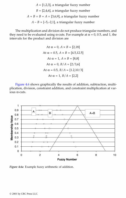
A = [1,2,3], a triangular fuzzy number
B = [2,4,6], a triangular fuzzy number
A + B = B + A = [3,6,9], a triangular fuzzy number
A – B = [–5,–2,1], a triangular fuzzy number
The multiplication and division do not produce triangular numbers, andthey need to be evaluated using α-cuts. For example at α = 0, 0.5, and 1, theintervals for the product and division are
At α = 0, A × B = [2,18]
At α = 0.5, A × B = [4.5,12.5]
At α = 1, A × B = [8,8]
At α = 0, B/A = [2/3,6]
At α = 0.5, B/A = [1.2,10/3]
At α = 1, B/A = [2,2]
Figure 4.6 shows graphically the results of addition, subtraction, multi-plication, division, constraint addition, and constraint multiplication at var-ious α-cuts.
Figure 4.6a Example fuzzy arithmetic of addition.
0
0.1
0.2
0.3
0.4
0.5
0.6
0.7
0.8
0.9
1
0 2 4 6 8 10
Fuzzy Number
Mem
ber
ship
Val
ue
A B A+B
© 2001 by CRC Press LLC

4.2.3.5 Operations on fuzzy setsIn this section, basic operations that can be used for fuzzy sets and eventsare introduced. These operations are defined in an analogous form to thecorresponding operations of crisp sets in Section 4.2.2.6.
Figure 4.6b Example fuzzy arithmetic of subtraction.
Figure 4.6c Example fuzzy arithmetic of multiplication.
0
0.1
0.2
0.3
0.4
0.5
0.6
0.7
0.8
0.9
1
-6 -4 -2 0 2 4 6 8
Fuzzy Number
Mem
ber
ship
Val
ue
A BA-B
0
0.1
0.2
0.3
0.4
0.5
0.6
0.7
0.8
0.9
1
0 5 10 15 20
Fuzzy Number
Mem
ber
ship
Val
ue
A B A*B
© 2001 by CRC Press LLC
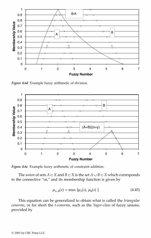
The union of sets A ⊂ X and B ⊂ X is the set A ∪ B ⊂ X which correspondsto the connective “or,” and its membership function is given by
µA∪B(x) = max [µA(x), µB(x) ] (4.45)
This equation can be generalized to obtain what is called the triangularconorms, or for short the t-conorms, such as the Yager-class of fuzzy unions,provided by
Figure 4.6d Example fuzzy arithmetic of division.
Figure 4.6e Example fuzzy arithmetic of constraint addition.
0
0.1
0.2
0.3
0.4
0.5
0.6
0.7
0.8
0.9
1
0 1 2 3 4 5 6 7
Fuzzy Number
Mem
ber
ship
Val
ue
A B
B/A
0
0.1
0.2
0.3
0.4
0.5
0.6
0.7
0.8
0.9
1
0 1 2 3 4 5 6 7
Fuzzy Number
Mem
ber
ship
Val
ue A
B
(A+B)|(x=y)
© 2001 by CRC Press LLC

µA∪B(x) = (4.46)
where β ∈(0, ∞) is called the intensity factor. Equation 4.46 reduces toEquation 4.45 as β → ∞. The union based on Equation 4.46 depends on β,and can take any value in the following range with lower and upper limitsthat correspond to β → ∞ and β → 0, respectively:
max(µA(x), µA(x)) ≤ µA∪B(x) ≤ (4.47)
The intersection of sets A ⊂ X and B ⊂ X is the set A ∩ B ⊂ X whichcorresponds to the connective “and,” and its membership function is givenby
µA∩B(x) = min [(µA(x), (µB(x)] (4.48)
This equation can be generalized to obtain what is called the triangularnorms, or for short the t-norms, such as the Yager-class of fuzzy intersections,provided by
Figure 4.6f Example fuzzy arithmetic of constraint multiplication.
0
0.1
0.2
0.3
0.4
0.5
0.6
0.7
0.8
0.9
1
0 2 4 6 8 10
Fuzzy Number
Mem
ber
ship
Val
ue A
B
(A*B)|(x=y)
min 1, µ µββ
A Bx x( )( ) + ( )( )
µ µ
µ µA B
B A
x x
x x
( ) ( ) =
( ) ( ) =
if
if
1 otherwise
0
0
© 2001 by CRC Press LLC

µA∩B(x) = (4.49)
where β ∈ (0,∞) is called the intensity factor. Equation 4.49 reduces toEquation 4.48 as β → ∞. The intersection based on Equation 4.49 dependson β , and can take any value in the following range with lower and upperlimits that correspond to β → 0 and β → ∞, respectively:
≤ µA∩B(x) ≤ min(µA(x), µB(x)) (4.50)
The difference between events A and B is the set A – B of all elementsthat belong to A but do not belong to B. The difference is mathematicallyexpressed as
µA–B(x) = (4.51)
The membership function of the complement A of a fuzzy set A is givenby
µA(x) = 1 – µA(x) (4.52)
This equation can be generalized to obtain the Yager-class of fuzzy com-plements as follows:
(4.53)
where β ∈ (0,∞) is called the intensity factor. Equation 4.53 reduces toEquation 4.52 for β = 1. The definition of the complement can be generalizedas provided, for example, by the Sugeno-class of fuzzy complements as fol-lows:
(4.54)
where β ∈ (0,∞) is called the intensity factor. Equation 4.54 reduces toEquation 4.52 as β = 0. The selection of a β value in the generalized defini-tions of fuzzy set operations requires the use of experts to calibrate these
1 – min 1 1 1, − ( )( ) + − ( )( )
µ µβ ββ
A Bx x
µ µ
µ µA B
B A
x x
x x
( ) ( ) =
( ) ( ) =
if
if
0 otherwise
1
1
µ µ
µA B
B
x x
x
( ) ( ) =
( ) ≠
if
0 if
0
0
µ µβ
ββA Ax x( ) = ( )( )1 –
µµ
βµβA
A
A
xx
x( ) =
( )+ ( )
1
1
–
© 2001 by CRC Press LLC

operations based on the context of use and application. The generalizeddefinitions according to Equations 4.46, 4.49, 4.53, and 4.54 contain softerdefinitions of union, intersection and complement, whereas the definitionsof the union, intersection, and complement of Equations 4.45, 4.48, and 4.52offer hard definitions. The generalized unions and intersections for two fuzzysets produce membership values as shown in Figure 4.7.
Figure 4.7 shows averaging, also called aggregation, operations that spanthe gap between the unions and intersections (Klir and Folger, 1988; Klir andWierman, 1999). An example of generalized aggregation is the generalizedmeans and is defined by
(4.55)
where ∇ is the generalized means aggregation operator, and β is an inten-sity factor whose range is the set of all real numbers excluding 0. Equation4.55 becomes the geometric mean as β → 0, and becomes
(4.56)
Equation 4.55 converges to the min and max operations as β → – ∞ andβ → ∞, respectively. Figure 4.7 shows this convergence.
Other generalized operations and additional information on this subjectare provided by Klir and Folger (1988), Klir and Wierman (1999), Yager(1980a), Schweizer and Sklar (1983), Frank (1979), Dubois and Prade (1980),and Dombi (1982).
Figure 4.7 Generalized fuzzy operations.
µ µ µβ ββ
A B A Bx x x∇ ( ) = ( )( ) + ( )( )12
µ µ µA B A Bx x x∇ ( ) = ( ) ( )
IntersectionOperations
( ) ( )-+--
∩
β ββ µµ
µ
)(1)(1,1min1 xx BA
BA
=
=
otherwise
xifx
xifx
AB
BA
0
1)()(
1)()(
µµµµ
))(),(min (µ xx BA µ
=→ ∩ )(,0 xAs BAµβ
=∞→ )(, xAs A∩Bµβ
UnionOperations
( ) ( )+
=∪β ββ µµ
µ
)()(,1min
)(
xx
x
BA
BA
=
=
otherwise
xifx
xifx
AB
BA
1
0)()(
0)()(
µµµµ
( ))(),(max xx BA µµ
=→ ∪ )(,0 xAs BAµβ
=∞→ ∪ )(, xAs BAµβ
GeneralizedMeans
( ) ( )β ββ µµ
µ
)()(2
1
)(
xx
x
BA
BA
+
=∇
( ))(),(min xx BA µµ=-∞→ ∇ )(, xAs BAµβ
( ))(),(max xx BA µµ=∞→ ∇ )(, xAs BAµβ
)(x =
© 2001 by CRC Press LLC

Example 4.9 Operations on fuzzy experience levels
Two experts provided the following assessments of long experience usingfuzzy sets B and C:
long experience,B = { 100 | 1. , 90 | 0.9 , 80 | 0.7 , 70 | 0.2 , 60 | 0.1 } (4.57)
long experience,C = { 100 | 1. , 90 | 0.8 , 80 | 0.6 , 70 | 0.4 , 60 | 0.2 } (4.58)
The union and intersection of these two sets can be computed accordingto Equations 4.45 and 4.48, respectively, to obtain the following:
B ∪ C = {100 | 1. , 90 | 0.9 , 80 | 0.7 , 70 | 0.4 , 60 | 0.2 } (4.59)
B ∩ C = {100 | 1. , 90 | 0.8 , 80 | 0.6 , 70 | 0.2 , 60 | 0.1 } (4.60)
The above definitions of the union and intersection of fuzzy sets are thehard definitions. The difference of the two sets is the empty set, and can bestated as
B – C = Ø (4.61)
The complement of B according to Equation 4.52 is given by
µB(x) = {90 | 0.1 , 80 | 0.3 , 70 | 0.8 , 60 | 0.9 , 50 | 1. , 40 | 1. , 30 | 1. , 20 | 1. , 10 | 1. , 0 | 1. } (4.62)
The α-cut of B at α = 0.7 according to Equation 4.28 is given by an intervalof real values as follows:
B0.7 = [80 , 100] (4.63)
Example 4.10 Additional operations on fuzzy sets
Figure 4.8 shows example fuzzy operations on two fuzzy events A and B.The intersection and union are shown using the min and max rules ofEquations 4.48 and 4.45, respectively. The complement is also shown basedon Equation 4.52. The last two figures show the unique properties of fuzzysets of A ∪ A ≠ S and A ∩ A ≠ Ø.
© 2001 by CRC Press LLC
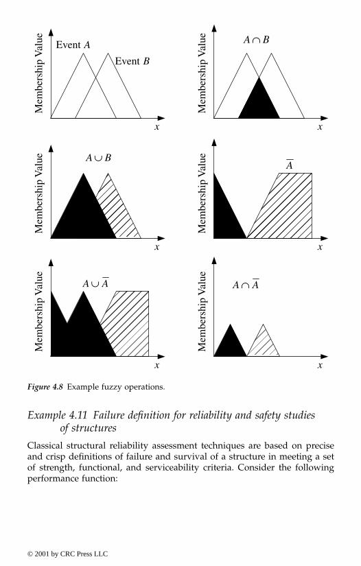
Example 4.11 Failure definition for reliability and safety studiesof structures
Classical structural reliability assessment techniques are based on preciseand crisp definitions of failure and survival of a structure in meeting a setof strength, functional, and serviceability criteria. Consider the followingperformance function:
Figure 4.8 Example fuzzy operations.
Event A
Event B
x
Mem
bers
hip
Val
ue
x
Mem
bers
hip
Val
ue BA ∩
x
Mem
bers
hip
Val
ue BA ∪
x
Mem
bers
hip
Val
ue A
x
Mem
bers
hip
Val
ue AA ∪
x
Mem
bers
hip
Val
ue
AA ∩
© 2001 by CRC Press LLC

Z = g(X1, X2, . . ., Xn) (4.64)
where X1, X2, . . ., Xn = basic random variables, and Z = performancemeasure or safety margin as the difference between structural strength as aresponse (R) to loads and the applied loads (L) (i.e., Z = R – L). Both R andL are functions of the basic random variables. Equation 4.64 is defined suchthat failure occurs where Z < 0, survival occurs where Z > 0, and the limitstate equation is defined as Z = 0. The probability of failure can then bedetermined by solving the following integral:
Pf = fX(x1,x2, . . ., xn) dx1,dx2, . . .dxn (4.65)
where fX is the joint probability density function of {X1, X2, . . ., Xn}, andthe integration is performed over the region where Z < 0 (Ayyub andMcCuen, 1997; Ayyub and Haldar, 1984; White and Ayyub, 1985).
The model for crisp failure consists of two basic, mutually exclusiveevents, i.e., complete survival and complete failure. The transition from oneto another is abrupt rather than continuous. This model is illustrated inFigure 4.9, where Rf is the structural response at the limiting state for aselected design criterion. If the structural response R is smaller than Rf, i.e.,R < Rf, the complete survival state exists and it is mapped to the zero failurelevel (α = 0). If the structural response R is larger than Rf, i.e., R > Rf, thecomplete failure state occurs and it is mapped to α = 1. The limit state isdefined where R = Rf.
The fuzzy failure model is illustrated by introducing a subjective failurelevel index α as shown in Figure 4.10, where RL and RR are the left (lower)bound and right (upper) bound of structural response for the region oftransitional or partial failure, respectively. The complete survival state isdefined where R ≤ RL, the response in the range (RL < R < RU) is the transi-tional state, and the response (R ≥ RU) is the complete failure state. In Figure4.10, the structural response is mapped to the failure-level scale to modelsome performance event as follows:
Performance event A: R → A = {α : α ∈ [0,1]} (4.66)
where 0 = failure level for complete survival, 1 = failure level for com-plete failure, and [0, 1] = all real values in the range of 0 to 1 for all failurelevels.
The index α can also be interpreted as a measure of degree of belief inthe occurrence of some performance condition. In this case, α = 0 is inter-preted as no belief of the occurrence of an event, and the α = 1 means absolutebelief of the occurrence of the event.
A mathematical model for structural reliability assessment that includesboth ambiguity and vagueness types of uncertainty was suggested by Alvi
L∫∫∫
© 2001 by CRC Press LLC

and Ayyub (1990) and Ayyub and Lai (1992 and 1994). The model results inthe likelihood of failure over a damage spectrum. Since the structural reli-ability assessment is based on the fuzzy failure model, the probability offailure, in this case, is a function of α. Figure 4.11 shows various grades offailures expressed as fuzzy events as used by Ayyub and Lai (1992) to assessthe structural reliability of ship hull girders.
Figure 4.9 A crisp failure definition.
Figure 4.10 A fuzzy failure definition.
0
0.25
0.5
0.75
1
Structural Response, such as, Deflection
Mem
ber
ship
Val
ue
R f
Crisp Failure
0
0.25
0.5
0.75
1
Structural Response, such as, Deflection
Mem
ber
ship
Val
ue
R fL R fR
Fuzzy Failure
© 2001 by CRC Press LLC

4.2.3.6 Fuzzy relationsA relation between two or more sets is defined as an expression of associa-tion, interrelationship, interconnection, or interaction among these sets. Theexpression can be made in a crisp format indicating the presence or absenceof such a relation, or it can be made in a fuzzy format indicating the degreeof belief in the presence or absence of the relation. A degree of belief in arelationship R between x ∈ X and y ∈ Y is commonly expressed using µR(x,y)∈ [0,1]. If µR(x,y) ∈ {0,1}, i.e., µR(x,y) can take one of two values 0 or 1, thenR is considered to be a crisp relation; whereas if µR(x,y) ∈ [0,1], i.e., µR(x,y)can take any real value in the range [0,1], then R is considered to be a fuzzyrelation.
A fuzzy relation R between two sets A ⊂ X and B⊂ Y can be defined onthe Cartesian product of A and B as the set of all ordered pairs (a,b) suchthat a ∈ A and b ∈ B, for discrete A and B. In mathematical notations, theCartesian product is expressed by the following space:
A × B = {(a,b): a ∈ A and b ∈ B} (4.67)
For continuous A and B, the Cartesian product can be shown as a 2-dimensional x-y space over the ranges of A and B. The membership functionfor a fuzzy relation can be defined as
µR(a,b) = min [µA(a) , µB(b)] (4.68)
Figure 4.11 Fuzzy failure definitions for structural reliability assessment.
0
0.25
0.5
0.75
1
Structural Response, such as, Deflection
Mem
ber
ship
Val
ue
Survival ServiceabilityFailure
Partial Failure
Failure
Collapse
© 2001 by CRC Press LLC

For discrete A and B, relations are usually expressed in a matrix form asb1 b2 ... bm
a1 µR(a1,b1) µR(a1,b2) ... µR(a1,bm)
R = A × B = a2 µR(a2,b1) µR(a2,b2) ... µR(a2,bm) (4.69)
: : : : :an µR(an,b1) µR(an,b2) ... µR(an,bm)
in which A = {a1, a2, ..., an}; B = {b1, b2, ..., bm}; and µR(ai,bj) = support ormembership value for the ordered pair (ai,bj) that is a measure of associationbetween ai and bj. The membership value can be determined based on judg-ment or can be computed as the minimum value of the membership valuesµA(ai) and µB(bj).
A fuzzy relation can be expressed in a conditional form. For example,the relation R can be defined as
‘if experience of workers on a production line is short,then the quality of the product is medium.
Defining “short experience” and a “medium” product quality, respec-tively, as
short experience,A = { 40 | 0.1 , 30 | 0.5 , 20 | 0.7 , 10 | 0.9 , 0 | 1.0 } (4.70)
medium quality ={ 70 | 0.2 , 60 | 0.7 , 50 | 1. , 40 | 0.7 , 30 | 0.2 } (4.71)
then, the fuzzy relation R can be computed as
short experience40 30 20 10 0
medium 70 0.1 0.2 0.2 0.2 0.2R = product 60 0.1 0.5 0.7 0.7 0.7 (4.72)
quality 50 0.1 0.5 0.7 0.9 1.040 0.1 0.5 0.7 0.7 0.730 0.1 0.2 0.2 0.2 0.2
Note that the fuzzy sets “short experience” and “medium product qual-ity” are from two different universes, namely, “experience” and “quality,”respectively. The membership values of the first row in Equation 4.72 wereevaluated as follows:
© 2001 by CRC Press LLC

µR(70 , 40) = min (0.2 , 0.1) = 0.1µR(70 , 30) = min (0.2 , 0.5) = 0.2µR(70 , 20) = min (0.2 , 0.7) = 0.2 (4.73)µR(70 , 10) = min (0.2 , 0.9) = 0.2µR(70 , 0) = min (0.2 , 1.0) = 0.2
The union of two relations, say R and S, is denoted by R ∪ S and hasthe following membership function:
µR∪S(x,y) = max[µR(x,y) , µS(x,y)] (4.74)
where both relations R and S are defined on the Cartesian product spaceX × Y. On the other hand, the intersection of two fuzzy relations, R ∩ S, hasthe following membership function:
µR∩S x,y) = min [µR(x,y) , µS(x,y)] (4.75)
These “hard” definitions of the union and intersection of two fuzzyrelations can be generalized to perform the union and intersection of severalrelations using the “max” and “min” operators, respectively. The hard def-initions of these operations can also be generalized using the Yager-classes,similar to the union and intersection of fuzzy sets.
Other operations on fuzzy relations include their complement and com-position. The complement R of fuzzy relation R has the following member-ship function:
µR (x,y) = 1 – µR(x,y) (4.76)
The composition of a fuzzy relation R defined on the universe X × Y anda fuzzy relation S defined on the universe Y × Z is the fuzzy relation R Sdefined on the universe X × Z. The membership function for this fuzzyrelation is given by
(4.77)
An interesting case of fuzzy composition is the composition of a fuzzysubset A defined on the universe X with a relation R defined on the universeX x Y. The result is a fuzzy subset B defined on the universe Y with amembership function given by
(4.78)
o
µ µ µR Sy Y
R Sx z x y y zo , , , ,( ) = ( ) ( )[ ]{ }∈max minall
µ µ µA Rx X
A Ry x x yo ( ) = ( ) ( )[ ]{∈max minall
, ,
© 2001 by CRC Press LLC
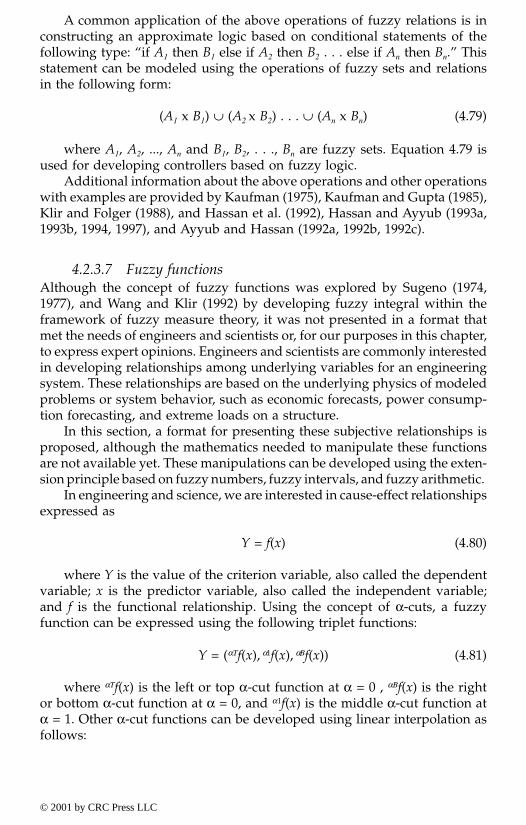
A common application of the above operations of fuzzy relations is inconstructing an approximate logic based on conditional statements of thefollowing type: “if A1 then B1 else if A2 then B2 . . . else if An then Bn.” Thisstatement can be modeled using the operations of fuzzy sets and relationsin the following form:
(A1 x B1) ∪ (A2 x B2) . . . ∪ (An x Bn) (4.79)
where A1, A2, ..., An and B1, B2, . . ., Bn are fuzzy sets. Equation 4.79 isused for developing controllers based on fuzzy logic.
Additional information about the above operations and other operationswith examples are provided by Kaufman (1975), Kaufman and Gupta (1985),Klir and Folger (1988), and Hassan et al. (1992), Hassan and Ayyub (1993a,1993b, 1994, 1997), and Ayyub and Hassan (1992a, 1992b, 1992c).
4.2.3.7 Fuzzy functionsAlthough the concept of fuzzy functions was explored by Sugeno (1974,1977), and Wang and Klir (1992) by developing fuzzy integral within theframework of fuzzy measure theory, it was not presented in a format thatmet the needs of engineers and scientists or, for our purposes in this chapter,to express expert opinions. Engineers and scientists are commonly interestedin developing relationships among underlying variables for an engineeringsystem. These relationships are based on the underlying physics of modeledproblems or system behavior, such as economic forecasts, power consump-tion forecasting, and extreme loads on a structure.
In this section, a format for presenting these subjective relationships isproposed, although the mathematics needed to manipulate these functionsare not available yet. These manipulations can be developed using the exten-sion principle based on fuzzy numbers, fuzzy intervals, and fuzzy arithmetic.
In engineering and science, we are interested in cause-effect relationshipsexpressed as
Y = f(x) (4.80)
where Y is the value of the criterion variable, also called the dependentvariable; x is the predictor variable, also called the independent variable;and f is the functional relationship. Using the concept of α-cuts, a fuzzyfunction can be expressed using the following triplet functions:
Y = (αTf(x), α1f(x), αBf(x)) (4.81)
where αTf(x) is the left or top α-cut function at α = 0 , αBf(x) is the rightor bottom α-cut function at α = 0, and α1f(x) is the middle α-cut function atα = 1. Other α-cut functions can be developed using linear interpolation asfollows:
© 2001 by CRC Press LLC

αf(x) = (4.82)
Fuzzy functions can be used to extrapolate empirical functions to regionsbeyond data availability, for example for developing forecasting models.Functional operations such as derivatives, integrals, roots, maximums, andminimums can be defined using the α-cut concepts. These computations canbe performed using numerical techniques performed on the function valuesat the α-cuts. Ayyub and McCuen (1996) describe commonly used numericalmethods with practical examples.
Example 4.12 Forecasting power needs using a fuzzy function
The power needs of a city can be forecasted to help city planners makezoning and power-plant construction decisions. Figure 4.12 shows an empir-ical power consumption trend over time and a subjectively developed fore-cast of the city’s needs. The forecasted segment of the curve is provided fordemonstration purposes. The following fuzzy function is used to developFigure 4.12:
(4.83)
where Year is in a four-digit number format. The figure shows the empir-ical data, and three functions that correspond to middle, and top and bottomat α-cuts of 0 and 1, respectively.
4.2.4 Fundamentals of rough sets
4.2.4.1 Rough set definitionsRough sets were introduced by Pawlak (1991) and are described with exam-ples by Pal and Skowron (1999). Rough sets provide the means to representimprecise classical (crisp) sets. The representation is based on a partition ofthe universal space involved that should be constructed to facilitate thisrepresentation. Each rough set represents a given crisp set by two subsetsof the partition, a lower approximation and an upper approximation. Thelower approximation consists of all subsets of the partition that are includedin the crisp set represented, whereas the upper approximation consists of allsubsets that overlap with the set represented. Figure 4.13 shows a crisp set
α α α α α α
α α α α α α
B B B
T T
f x a f x f x f x f x f x
f x a f x f x f x f x f x
( ) + ( ) ( )( ) ( )≤ ( )− ( )( ) + ( ) ( )( ) ( )≤ ( )− ( )
1 1
1 1 1
–
–
for
for
Y
f x Year
f x Year
f x Year
T
B
=
( ) = + ( )( ) = + ( )( ) = + ( )
α
α
α
233 5 5 2000
233 5 2000
233 5 2000 5
1
–
–
– /
© 2001 by CRC Press LLC
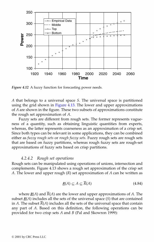
A that belongs to a universal space S. The universal space is partitionedusing the grid shown in Figure 4.13. The lower and upper approximationsof A are shown in the figure. These two subsets of approximations constitutethe rough set approximation of A.
Fuzzy sets are different from rough sets. The former represents vague-ness of a quantity, such as obtaining linguistic quantities from experts,whereas, the latter represents coarseness as an approximation of a crisp set.Since both types can be relevant in some applications, they can be combinedeither as fuzzy rough sets or rough fuzzy sets. Fuzzy rough sets are rough setsthat are based on fuzzy partitions, whereas rough fuzzy sets are rough-setapproximations of fuzzy sets based on crisp partitions.
4.2.4.2 Rough set operationsRough sets can be manipulated using operations of unions, intersection andcomplements. Figure 4.13 shows a rough set approximation of the crisp setA. The lower and upper rough (R) set approximation of A can be written as
R(A) ⊆ A ⊆ R(A) (4.84)
where R(A) and R(A) are the lower and upper approximations of A. Thesubset R(A) includes all the sets of the universal space (S) that are containedin A. The subset R(A) includes all the sets of the universal space that containany part of A. Based on this definition, the following operations can beprovided for two crisp sets A and B (Pal and Skowron 1999):
Figure 4.12 A fuzzy function for forecasting power needs.
100
150
200
250
300
350
1920 1940 1960 1980 2000 2020 2040 2060Time
Po
wer
Empirical DataMiddleTopBottom
© 2001 by CRC Press LLC

R(Ø) = Ø = R(Ø) (4.85)
R(S) = S = R(S) (4.86)
R(A ∪ B) = R(A) ∪ R(B) (4.87)
Figure 4.13 Rough set approximations.
a) Lower Approximation
b) Upper Approximation
© 2001 by CRC Press LLC
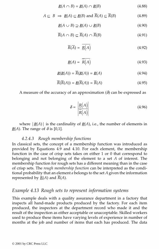
R(A ∩ B) = R(A) ∩ R(B) (4.88)
A ⊆ B ⇒ R(A) ⊆ R(B) and R(A) ⊆ R(B) (4.89)
R(A ∪ B) ⊇ R(A) ∪ R(B) (4.90)
R(A ∩ B) ⊆ R(A) ∩ R(B) (4.91)
R(A) = (4.92)
R(A) = (4.93)
R(R(A)) = R(R(A)) = R(A) (4.94)
R(R(A)) = R(R(A)) = R(A) (4.95)
A measure of the accuracy of an approximation (δ) can be expressed as
δ = (4.96)
where |R(A)| is the cardinality of R(A), i.e., the number of elements inR(A). The range of δ is [0,1].
4.2.4.3 Rough membership functionsIn classical sets, the concept of a membership function was introduced asprovided by Equations 4.9 and 4.10. For each element, the membershipfunction in the case of crisp sets takes on either 1 or 0 that correspond tobelonging and not belonging of the element to a set A of interest. Themembership function for rough sets has a different meaning than in the caseof crisp sets. The rough membership function can be interpreted as the condi-tional probability that an element a belongs to the set A given the informationrepresented by R(A) and R(A).
Example 4.13 Rough sets to represent information systems
This example deals with a quality assurance department in a factory thatinspects all hand-made products produced by the factory. For each itemproduced, the inspectors at the department record who made it and theresult of the inspection as either acceptable or unacceptable. Skilled workersused to produce these items have varying levels of experience in number ofmonths at the job and number of items that each has produced. The data
R A( )
R A( )
R A
R A
( )( )
© 2001 by CRC Press LLC

shown in Table 4.3 were collected based on inspecting ten items. For eachitem, the table shows the experience level of the person who made the item(measured as the number of years at the job and number of items the personhas produced), and the outcome of the inspection. Representing each itemby its pair of the number of months and number of items, Figure 4.14 canbe developed using rough sets. The figure shows x1, x2, x3, x8 and x10 as itemsthat are unacceptable, x4 and x5 as borderline items of the rough set that areeither acceptable or unacceptable, and x6, x7, and x9 as items that are accept-able. Based on this figure, the following rough set of unacceptable items (A)can be defined:
R(A) = {x1, x2, x3, x8, x10} (4.97)R(A) = {x1, x2, x3, x4, x5, x8, x10}
Similarly, the following rough set of acceptable items (A) can be defined:
R(A) = {x6, x7, x9} (4.98)R(A) = {x4, x5, x6, x7, x9}
These rough sets are shown in Figure 4.14.
4.2.4.4 Rough functionsThe concept of rough functions was introduced by Pawlak (1999) to presenta coarse approximation of unknown functions. Rough functions can be aneffective means to meet the needs of engineers and scientists for our purposesin this chapter to express expert opinions. In developing relationships amongvariables underlying an engineering system, these rough functions can beused to articulate and express the opinion of experts in cases, such as foreconomic forecasts, power consumption forecasting, and assessing extremeloads on a structure.
Table 4.3 Inspection Data for Quality
Item Number
Experience(Number of
Months)
Experience(Number of
Items Produced)InspectionOutcome
x1 5 10 Unacceptablex2 5 10 Unacceptablex3 12 5 Unacceptablex4 12 12 Acceptablex5 12 12 Unacceptablex6 20 10 Acceptablex7 24 12 Acceptablex8 6 8 Unacceptablex9 18 10 Acceptablex10 10 10 Unacceptable
© 2001 by CRC Press LLC
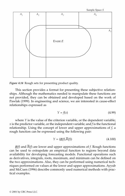
This section provides a format for presenting these subjective relation-ships. Although the mathematics needed to manipulate these functions arenot provided, they can be obtained and developed based on the work ofPawlak (1999). In engineering and science, we are interested in cause-effectrelationships expressed as
Y = f(x) (4.99)
where Y is the value of the criterion variable, or the dependent variable;x is the predictor variable, or the independent variable; and f is the functionalrelationship. Using the concept of lower and upper approximations of f, arough function can be expressed using the following pair:
Y = (R(f),R(f)) (4.100)
R(f) and R(f) are lower and upper approximations of f. Rough functionscan be used to extrapolate an empirical function to regions beyond dataavailability for developing forecasting models. Functional operations suchas derivatives, integrals, roots, maximum, and minimum can be defined onthe two approximations. Also, they can be performed using numerical tech-niques performed on values at the lower and upper approximations. Ayyuband McCuen (1996) describe commonly used numerical methods with prac-tical examples.
Figure 4.14 Rough sets for presenting product quality.
A1 A2 A3 A4
A5
Event E
Sample Space S
© 2001 by CRC Press LLC

Example 4.14 Forecasting power needs using a rough function
The power needs of a city can be forecasted to help city planners in makingzoning and power-plant construction decisions as discussed in Example 4.12.Figure 4.15 shows an empirical power consumption trend over time and asubjectively developed forecast of the city’s needs using lower and upperapproximations of the needs (f). The forecasted segment of the curve isprovided for demonstration purposes. The rough function was developedby establishing convenient gridlines, every 10 units of power and every fiveyears as shown Figure 4.15. Then, lower and upper approximation of thecity’s unknown needs for power by identifying the coordinate points thatwould include the unknown function.
4.3 Monotone measuresMonotone measures are often referred to in the literature as fuzzy measures(Wang and Klir, 1992; Klir and Wierman, 1999), although fuzzy sets are notnecessarily involved in the definition of these measures. The concept ofmonotone measures was conceived by Sugeno (1974). Monotone measurescan also be developed for fuzzy sets, and this case should be called fuzzymeasures.
Monotone measures are needed to model inconsistency and incomplete-ness ignorance types as shown in Figure 1.9. They can be used to modeluncertainty in the membership of an element of a universal set X to a family
Figure 4.15 A rough function for forecasting power needs.
100120140160180200220240260280300320340
1920 1940 1960 1980 2000 2020 2040 2060Time
Po
wer
Empirical DataUnknown City NeedsUpper ApproximationLower Approximation
© 2001 by CRC Press LLC

of sets that are identified by an analyst for the convenience of capturingand expressing opinions. The membership uncertainty in this case is differ-ent from the membership functions of fuzzy sets. While fuzzy sets havemembership functions to represent uncertainty in belonging to a set of fuzzyboundaries or a vague concept, monotone measures provide an assessmentof the membership likelihood of an element of X to each set in the familyof sets identified by the analyst. The family of sets are crisp sets, whereasthe element is imprecise in its boundaries and hence uncertain in its belong-ing to the sets of the family of sets. In fuzzy sets, the elements of X are crispand precise, but a set of interest is vague or fuzzy, hence the uncertainty.An example of a situation where monotone measures can be used is in filinga historical failure case of a system to predetermined, precisely defined,classes of failure causes. The failure case at hand might have a complexcause that would make classifying it to only one failure-cause class unreal-istic and would make its classification possible only in the form of a mono-tone measure, i.e., likelihood of belonging, to each of the prescribed failureclasses.
4.3.1 Definition of monotone measures
A monotone measure can be defined based on a nonempty family A of subsetsfor a given universal set X, with an appropriate algebraic structure as amapping from A to [0,∞] as follows:
f: A → [0,∞] (4.101)
The monotone measure must vanish at the empty set as follows:
f(∅) = 0 (4.102)
For all A1 and A2 ∈ A, and A1 ⊆ A2, then f(A1) ≤ f(A2), i.e., monotonicsets. For any increasing sequence A1 ⊆ A2 ⊆ . . . of sets in A, the function fis continuous from below, and for any decreasing sequence A1 ⊇ A2 ⊇ . . . ofsets in A, the function f is continuous from above. Functions that satisfy theabove four requirements are called semicontinuous from below or above,respectively. For any pair A1 and A2 ∈ A such that A1 ∩ A2 = ∅, a monotonemeasure f can have one of the following properties as provided by Equations4.103 – 4.105:
f(A1 ∪ A2) > f(A1) + f(A2) (4.103)
Equation 4.103 can be viewed as expressing a cooperative action or synergybetween A1 and A2.
f(A1 ∪ A2) = f(A1) + f(A2) (4.104)
© 2001 by CRC Press LLC

Equation 4.104 can be viewed as expressing a noninteractive nature of A1
and A2.
f(A1 ∪ A2) < f(A1) + f(A2) (4.105)
Equation 4.105 can be viewed as expressing an inhibitory effect or incom-patibility between A1 and A2 (Wang and Klir, 1992; Klir and Wierman, 1999).Probability theory is based on a classical measure theory as provided byEquation 4.104. Therefore, the theory of monotone measures provides abroader framework than probability theory for modeling uncertainty. In fact,monotone measures are general enough to encompass probability theory,possibility theory, and theory of evidence.
4.3.2 Classifying monotone measures
A two-way classification of monotone measures can be developed based onthe work of Wang and Klir (1992) and Klir and Wierman (1999), using thefollowing two considerations: (1) the type of sets (crisp, fuzzy and/or rough),and (2) the properties provided by Equations 4.103 – 4.105. The Cartesiancombination of these two considerations would produce many types ofmonotone measures that are not all fully developed in the literature. Thereasonably developed types of monotone measures are listed below.
1. Classical probability theory. Classical probability theory is based oncrisp sets and additive measures, i.e., Equation 4.104.
2. Probability theory based on fuzzy events (fuzzy sets and additivemeasures, i.e., Equation 4.104). In this case classical probability con-cepts are extended to deal with fuzzy events as demonstrated byAyyub and Lai (1994).
3. Dempster-Shafer theory of evidence and its monotone measures ofbelief and plausibility (crisp sets and nonadditive measures, i.e.,Equations 4.103 and 4.105). This is the classic case of the Dempster-Shafer theory of evidence (Shafer, 1976; Dempster, 1976a, 1976b). Thetheory of evidence defines and uses two monotone measures calledbelief and plausibility measures that form a dual.
4. Fuzzified Dempster-Shafer theory of evidence (fuzzy sets and non-additive measures, i.e., Equations 4.103 and 4.105). This is an exten-sion of the classic case of the Dempster-Shafer theory of evidence byconsidering fuzzy sets.
5. Possibility theory and its monotone measures of necessity and possibil-ity (crisp sets and nonadditive measures, i.e., Equations 4.103 and4.105). This possibility theory case is a special case of the aboveDempster-Shafer theory of evidence and its monotone measures ofbelief and plausibility by requiring underlying events to be nested,i.e., A1 ⊂ A2 ⊂ . . . ⊂ X.
© 2001 by CRC Press LLC
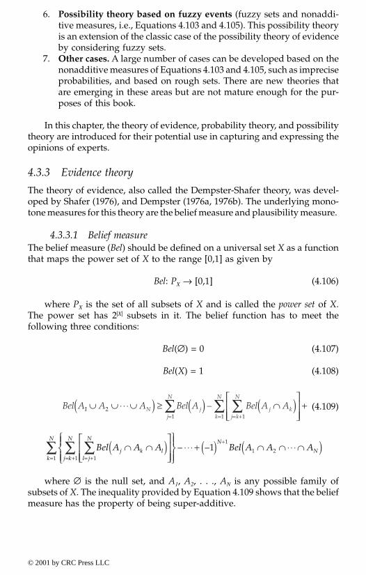
6. Possibility theory based on fuzzy events (fuzzy sets and nonaddi-tive measures, i.e., Equations 4.103 and 4.105). This possibility theoryis an extension of the classic case of the possibility theory of evidenceby considering fuzzy sets.
7. Other cases. A large number of cases can be developed based on thenonadditive measures of Equations 4.103 and 4.105, such as impreciseprobabilities, and based on rough sets. There are new theories thatare emerging in these areas but are not mature enough for the pur-poses of this book.
In this chapter, the theory of evidence, probability theory, and possibilitytheory are introduced for their potential use in capturing and expressing theopinions of experts.
4.3.3 Evidence theory
The theory of evidence, also called the Dempster-Shafer theory, was devel-oped by Shafer (1976), and Dempster (1976a, 1976b). The underlying mono-tone measures for this theory are the belief measure and plausibility measure.
4.3.3.1 Belief measureThe belief measure (Bel) should be defined on a universal set X as a functionthat maps the power set of X to the range [0,1] as given by
Bel: PX → [0,1] (4.106)
where PX is the set of all subsets of X and is called the power set of X.The power set has 2|X| subsets in it. The belief function has to meet thefollowing three conditions:
Bel(∅) = 0 (4.107)
Bel(X) = 1 (4.108)
(4.109)
where ∅ is the null set, and A1, A2, . . ., AN is any possible family ofsubsets of X. The inequality provided by Equation 4.109 shows that the beliefmeasure has the property of being super-additive.
Bel A A A Bel A Bel A AN jj
N
j kj k
N
k
N
1 ∪ ∪ ⋅⋅ ⋅ ∪( ) ≥ ( ) ∩( )
+= = +=∑ ∑∑2
1 11
–Bel A A A Bel A Bel A AN jj
N
j kj k
N
k
N
1 ∪ ∪ ⋅⋅ ⋅ ∪( ) ≥ ( ) ∩( )
+= = +=∑ ∑∑2
1 11
–
Bel A A A Bel A A Aj k ll j
N
j k
N
k
N N
N∩ ∩( )
⋅ ⋅ ⋅ + ( ) ∩ ∩ ⋅⋅ ⋅ ∩( )
= += +=
+∑∑∑111
1
1 21– –
© 2001 by CRC Press LLC

4.3.3.2 Plausibility measureThe belief measure (Bel) has a dual measure called the plausibility measure(Pl) as defined by the following equation:
Pl(A) = 1 − Bel(A) (4.110)
where A is a subset that belongs to the power set PX. The plausibilitymeasure must satisfy the following conditions:
Pl(∅) = 0 (4.111)
Pl(X) = 1 (4.112)
(4.113)
where A1, A2, …, AN is any family of subsets of X. The pair, Bel and Pl,forms a duality. The inequality provided by Equation 4.113 shows that theplausibility measure has the property of being sub-additive. It can be shownthat the belief and plausibility functions satisfy the following condition:
Pl(A) > Bel(A) (4.114)
for each A in the power set.
4.3.3.3 Basic assignmentIn engineering and science, a body of evidence represented by a family ofsets (A1, A2, . . ., AN) can be characterized by a basic assignment constructedfor convenience and for facilitating the expression and modeling of, forexample, expert opinions. A basic assignment can be related to the beliefand plausibility measures; however, its creation is commonly easier andmore relevant to problems than directly developing the belief and plausibil-ity measures. A basic assignment provides an assessment of the membershiplikelihood of an element x of X to each set in a family of sets identified bythe analyst. The family of sets are crisp sets, whereas the element of interestx is imprecise in its boundaries and hence uncertain in its belonging to thesets in the family of sets.
A basic assignment can be conveniently characterized by the followingfunction that maps the power set to the range [0,1]:
m: PX → [0,1] (4.115)
Pl A A A Pl A Pl A AN jj
N
j kj k
N
k
N
1 ∩ ∩ ⋅⋅ ⋅ ∩( ) ≤ ( ) ∪( )
+ ⋅ ⋅ ⋅= ==∑ ∑∑2
1 1
–
+( ) ∪ ∪ ⋅⋅ ⋅ ∪( )+–1
1
1 2
N
NPl A A A
© 2001 by CRC Press LLC
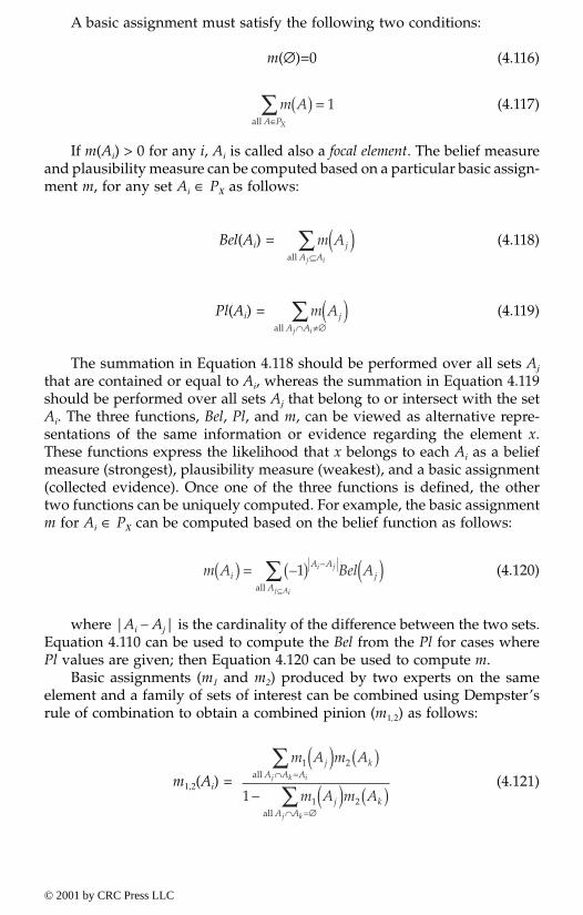
A basic assignment must satisfy the following two conditions:
m(∅)=0 (4.116)
(4.117)
If m(Ai) > 0 for any i, Ai is called also a focal element. The belief measureand plausibility measure can be computed based on a particular basic assign-ment m, for any set Ai ∈ PX as follows:
Bel(Ai) = (4.118)
Pl(Ai) = (4.119)
The summation in Equation 4.118 should be performed over all sets Aj
that are contained or equal to Ai, whereas the summation in Equation 4.119should be performed over all sets Aj that belong to or intersect with the setAi. The three functions, Bel, Pl, and m, can be viewed as alternative repre-sentations of the same information or evidence regarding the element x.These functions express the likelihood that x belongs to each Ai as a beliefmeasure (strongest), plausibility measure (weakest), and a basic assignment(collected evidence). Once one of the three functions is defined, the othertwo functions can be uniquely computed. For example, the basic assignmentm for Ai ∈ PX can be computed based on the belief function as follows:
(4.120)
where |Ai – Aj| is the cardinality of the difference between the two sets.Equation 4.110 can be used to compute the Bel from the Pl for cases wherePl values are given; then Equation 4.120 can be used to compute m.
Basic assignments (m1 and m2) produced by two experts on the sameelement and a family of sets of interest can be combined using Dempster’srule of combination to obtain a combined pinion (m1,2) as follows:
m1,2(Ai) = (4.121)
m AA PX
( ) =∈
∑ 1all
m AjA Aj i
( )⊆
∑all
m AjA Aj i
( )∩ ≠∅∑
all
m A Bel AiA A
Aj
i j
j Ai
( ) = ( ) ( )⊆
∑ – –1all
m A m A
m A m A
j kA A A
j kA A
j k i
j k
1 2
1 21
( ) ( )
− ( ) ( )∩ =
∩ =∅
∑
∑all
all
© 2001 by CRC Press LLC
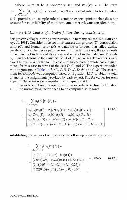
where Ai must be a nonempty set, and m1,2(Ø) = 0. The term
of Equation 4.121 is a normalization factor. Equation
4.121 provides an example rule to combine expert opinions that does notaccount for the reliability of the source and other relevant considerations.
Example 4.15 Causes of a bridge failure during construction
Bridges can collapse during construction due to many causes (Eldukair andAyyub, 1991). Consider three common causes: design error (D), constructionerror (C), and human error (H). A database of bridges that failed duringconstruction can be developed. For each bridge failure case, the case needsto be classified in terms of its causes and entered in the database. The setsD, C, and H belong to the universal set X of failure causes. Two experts wereasked to review a bridge-failure case and subjectively provide basic assign-ments for this case in terms of the sets D, C, and H. The experts providedthe assignments in Table 4.4 for D, C, H, D∪C, D∪H, and C∪H. The assign-ment for D∪C∪H was computed based on Equation 4.117 to obtain a totalof one for the assignments provided by each expert. The Bel values for eachexpert in Table 4.4 were computed using Equation 4.118.
In order to combine the opinions of the experts according to Equation4.121, the normalizing factor needs to be computed as follows:
(4.122)
substituting the values of m produces the following normalizing factor:
= 0.8675 (4.123)
1 1 2− ( ) ( )∩ =∅∑m A m Aj k
A Aj kall
1
1
1 2
1 2 1 2 1 2
1 2 1 2 1 2
1 2 1 2
− ( ) ( ) =
( ) ( ) + ( ) ( ) + ( ) ∪( ) +( ) ( ) + ( ) ( ) + ( ) ∪( ) +( ) ( ) + ( ) ( )
∩ =∅∑m A m A
m D m C m D m H m D m C H
m C m D m C m H m C m D H
m H m D m H m C
j kA Aj kall
–++ ( ) ∪( ) +
∪( ) ( ) + ∪( ) ( ) + ∪( ) ( )
m H m C D
m D C m H m D H m C m C H m D1 2
1 2 1 2 1 2
1
1
0 1 0 1 0 1 0 15 0 1 0 10 05 0 05 0 05 0 15 0 05 0 10 1 0 05 0 1 0 1 0 1 0 25
1 2− ( ) ( ) =
( ) + ( ) + ( ) +( )( ) + ( )( ) + ( )( ) +( )( ) + ( )( ) + ( )(
∩ =∅∑m A m Aj k
A Aj kall
–
. . . . . .
. . . . . .
. . . . . . )) +( )( ) + ( )( ) + ( )( )
0 2 0 15 0 1 0 1 0 05 0 05. . . . . .
© 2001 by CRC Press LLC
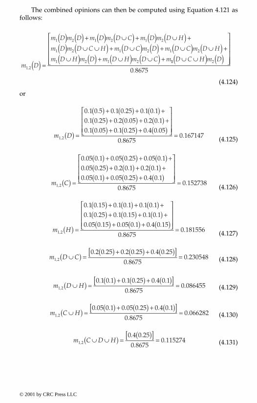
The combined opinions can then be computed using Equation 4.121 asfollows:
(4.124)
or
(4.125)
(4.126)
(4.127)
(4.128)
(4.129)
(4.130)
(4.131)
m D
m D m D m D m D C m D m D H
m D m D C H m D C m D m D C m D H
m D H m D m D H m D C m1 2
1 2 1 2 1 2
1 2 1 2 1 2
1 2 1 2
, ( ) =
( ) ( ) + ( ) ∪( ) + ( ) ∪( ) +
( ) ∪ ∪( ) + ∪( ) ( ) + ∪( ) ∪( ) +
∪( ) ( ) + ∪( ) ∪( ) + 11 2
0 8675
D C H m D∪ ∪( ) ( )
.
m D1 2
0 1 0 5 0 1 0 25 0 1 0 10 1 0 25 0 2 0 05 0 2 0 10 1 0 05 0 1 0 25 0 4 0 05
0 86750 167147,
. . . . . .
. . . . . .
. . . . . .
..( ) =
( ) + ( ) + ( ) +( ) + ( ) + ( ) +( ) + ( ) + ( )
=
m C1 2
0 05 0 1 0 05 0 25 0 05 0 10 05 0 25 0 2 0 1 0 2 0 10 05 0 1 0 05 0 25 0 4 0 1
0 86750 152738,
. . . . . .
. . . . . .
. . . . . .
..( ) =
( ) + ( ) + ( ) +( ) + ( ) + ( ) +( ) + ( ) + ( )
=
m H1 2
0 1 0 15 0 1 0 1 0 1 0 10 1 0 25 0 1 0 15 0 1 0 10 05 0 15 0 05 0 1 0 4 0 15
0 86750 181556,
. . . . . .
. . . . . .
. . . . . .
..( ) =
( ) + ( ) + ( ) +( ) + ( ) + ( ) +
( ) + ( ) + ( )
=
m D C1 2
0 2 0 25 0 2 0 25 0 4 0 25
0 86750 230548,
. . . . . .
..∪( ) =
( ) + ( ) + ( )[ ] =
m D H1 2
0 1 0 1 0 1 0 25 0 4 0 1
0 86750 086455,
. . . . . .
..∪( ) =
( ) + ( ) + ( )[ ] =
m C H1 2
0 05 0 1 0 05 0 25 0 4 0 1
0 86750 066282,
. . . . . .
..∪( ) =
( ) + ( ) + ( )[ ] =
m C D H1 2
0 4 0 25
0 86750 115274,
. .
..∪ ∪( ) =
( )[ ] =
© 2001 by CRC Press LLC

The values provided by Equations 4.125 – 4.131 must add up to one. TheBel1,2 values in Table 4.4 were computed using Equation 4.118. The plausi-bility computations for classifying bridge failures are shown in Table 4.5 thatwere based on Equation 4.119.
4.3.4 Probability theory
4.3.4.1 Relationship between evidence theory and probability theoryProbability theory can be treated as a special case of the theory of evidence.For cases in which all focal elements for a given basic assignment, m (i.e.,body of evidence) are singletons, the associated belief measure and plausi-bility measure collapse into a single measure, a classical probability measure.The term singleton means that each subset Ai of the family A of subsets,presenting an evidence body, contains only one element. The resulting prob-ability measure is additive in this case; i.e., it follows Equation 4.104. Thefollowing differences between evidence theory and probability theory canbe noted based on this reduction of evidence theory to probability theory:
Table 4.4 Belief Computations for Classifying Bridge Failures
Subset* Expert 1 Expert 2CombinedJudgment
(i.e., failure cause) m1 Bel1 m2 Bel2 m1,2 Bel1,2
Design error (D) 0.10 0.10 0.05 0.05 0.167147 0.167147Construction error (C) 0.05 0.05 0.10 0.10 0.152738 0.152738Human error (H) 0.10 0.10 0.15 0.15 0.181556 0.181556D ∪ C 0.20 0.35 0.25 0.40 0.230548 0.550433D ∪ H 0.10 0.30 0.10 0.30 0.086455 0.435158C ∪ H 0.05 0.20 0.10 0.35 0.066282 0.400576D ∪ C ∪ H 0.40 1. 0.25 1. 0.115274 1.
* The subsets could also be written as {D}, {C}, {H}, {D,C}, {D,H}, {C,H}, and {D,C,H}, respectively.
Table 4.5 Plausibility Computations for Classifying Bridge Failures
Subset* Expert 1 Expert 2CombinedJudgment
(i.e., failure cause) m1 Pl1 m2 Pl2 m1,2 Pl1,2
Design error (D) 0.10 0.80 0.05 0.65 0.167147 0.599424Construction error (C) 0.05 0.70 0.10 0.70 0.152738 0.564842Human error (H) 0.10 0.65 0.15 0.60 0.181556 0.449567D ∪ C 0.20 0.90 0.25 0.85 0.230548 0.818444D ∪ H 0.10 0.95 0.10 0.90 0.086455 0.847262C ∪ H 0.05 0.90 0.10 0.95 0.066282 0.832853D ∪ C ∪ H 0.40 1. 0.25 1. 0.115274 1.
* The subsets could also be written as {D}, {C}, {H}, {D,C}, {D,H}, {C,H}, and {D,C,H}, respectively.
© 2001 by CRC Press LLC
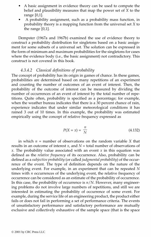
• A basic assignment in evidence theory can be used to compute thebelief and plausibility measures that map the power set of X to therange [0,1].
• A probability assignment, such as a probability mass function, inprobability theory is a mapping function from the universal set X tothe range [0,1].
Dempster (1967a and 1967b) examined the use of evidence theory toconstruct a probability distribution for singletons based on a basic assign-ment for some subsets of a universal set. The solution can be expressed inthe form of minimum and maximum probabilities for the singletons for caseswhere the evidence body (i.e., the basic assignment) not contradictory. Thisconstruct is not covered in this book.
4.3.4.2 Classical definitions of probabilityThe concept of probability has its origin in games of chance. In these games,probabilities are determined based on many repetitions of an experimentand counting the number of outcomes of an event of interest. Then, theprobability of the outcome of interest can be measured by dividing thenumber of occurrences of an event of interest by the total number of repe-titions. Quite often, probability is specified as a percentage; for example,when the weather bureau indicates that there is a 30 percent chance of rain,experience indicates that under similar meteorological conditions it hasrained 3 out of 10 times. In this example, the probability was estimatedempirically using the concept of relative frequency expressed as
P(X = x) = (4.132)
in which n = number of observations on the random variable X thatresults in an outcome of interest x, and N = total number of observations ofx. The probability value associated with an event x in this equation wasdefined as the relative frequency of its occurrence. Also, probability can bedefined as a subjective probability (or called judgmental probability) of the occur-rence of the event. The type of definition depends on the nature of theunderlying event. For example, in an experiment that can be repeated Ntimes with n occurrences of the underlying event, the relative frequency ofoccurrence can be considered as an estimate of the probability of occurrence.In this case, the probability of occurrence is n/N. However, many engineer-ing problems do not involve large numbers of repetitions, and still we areinterested in estimating the probability of occurrence of some event. Forexample, during the service life of an engineering product, the product eitherfails or does not fail in performing a set of performance criteria. The eventsof unsatisfactory performance and satisfactory performance are mutuallyexclusive and collectively exhaustive of the sample space (that is the space
nN
© 2001 by CRC Press LLC

of all possible outcomes). The probability of unsatisfactory performance (orsatisfactory performance) can be considered as a subjective probability.Another example is the failure probability of a dam because of an extremeflooding condition. Estimates of such probabilities can be achieved by mod-eling the underlying system, its uncertainties, and performances. The result-ing subjective probability is expected to reflect the status of our knowledgeabout the system regarding occurrence of the events of interest. Therefore,subjective probabilities can be associated with degrees of belief and can forma basis for Bayesian methods (Ayyub and McCuen, 1997). It is important tokeep in mind both definitions, so results are not interpreted beyond the rangeof their validity.
An axiomatic definition of probability is commonly provided in theliterature such as Ayyub and McCuen (1997). For an event A, the notationP(A) means the probability of occurrence of the event A. The probability Pshould satisfy the following axioms:
1. 0 < P(A) < 1, for any A that belongs to the set of all possible outcomes(called sample space S) for the system.
2. The probability of having S, P(S) = 1.3. The occurrence probability of the union of mutually exclusive events
is the sum of their individual occurrence probabilities.
The first axiom states that the probability of any event is inclusivelybetween 0 and 1. Therefore, negative probabilities, or probabilities largerthan one, are not allowed. The second axiom comes from the definition ofthe sample space. Since the sample space is the set of all possible outcomes,one or more of these outcomes must occur resulting in the occurrence of S.If the probability of the sample space does not equal 1, the sample spacewas incorrectly defined. The third axiom sets a basis for the mathematics ofprobability. These axioms as a single entity can be viewed as a definition ofprobability; i.e., any numerical structure that adheres to these axioms willprovide a probability structure. Therefore, the relative frequency and sub-jective probability meet this definition of probability.
Relative frequency and Subjective probability are tools that help engi-neers and planners to deal with and model uncertainty and should be usedappropriately as engineering systems and models demand. In the case ofrelative frequency, increasing the number of repetitions according to Equa-tion 4.132 would produce an improved estimate with a diminishing returnon invested computational and experimental resources until a limiting (i.e.long-run or long-term) frequency value is obtained. This limiting value canbe viewed as the true probability although the absolute connotation in thisterminology might not be realistic and cannot be validated. Philosophically,a true probability might not exist especially when dealing with subjectiveprobabilities. This, however, does not diminish the value of probabilisticanalysis and methods since they provide a consistent, systematic, rigorous,and robust framework for dealing with uncertainty and decision making.
© 2001 by CRC Press LLC
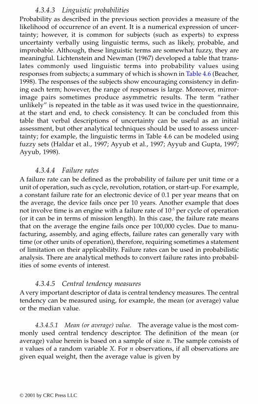
4.3.4.3 Linguistic probabilitiesProbability as described in the previous section provides a measure of thelikelihood of occurrence of an event. It is a numerical expression of uncer-tainty; however, it is common for subjects (such as experts) to expressuncertainty verbally using linguistic terms, such as likely, probable, andimprobable. Although, these linguistic terms are somewhat fuzzy, they aremeaningful. Lichtenstein and Newman (1967) developed a table that trans-lates commonly used linguistic terms into probability values usingresponses from subjects; a summary of which is shown in Table 4.6 (Beacher,1998). The responses of the subjects show encouraging consistency in defin-ing each term; however, the range of responses is large. Moreover, mirror-image pairs sometimes produce asymmetric results. The term “ratherunlikely” is repeated in the table as it was used twice in the questionnaire,at the start and end, to check consistency. It can be concluded from thistable that verbal descriptions of uncertainty can be useful as an initialassessment, but other analytical techniques should be used to assess uncer-tainty; for example, the linguistic terms in Table 4.6 can be modeled usingfuzzy sets (Haldar et al., 1997; Ayyub et al., 1997; Ayyub and Gupta, 1997;Ayyub, 1998).
4.3.4.4 Failure ratesA failure rate can be defined as the probability of failure per unit time or aunit of operation, such as cycle, revolution, rotation, or start-up. For example,a constant failure rate for an electronic device of 0.1 per year means that onthe average, the device fails once per 10 years. Another example that doesnot involve time is an engine with a failure rate of 10-5 per cycle of operation(or it can be in terms of mission length). In this case, the failure rate meansthat on the average the engine fails once per 100,000 cycles. Due to manu-facturing, assembly, and aging effects, failure rates can generally vary withtime (or other units of operation), therefore, requiring sometimes a statementof limitation on their applicability. Failure rates can be used in probabilisticanalysis. There are analytical methods to convert failure rates into probabil-ities of some events of interest.
4.3.4.5 Central tendency measuresA very important descriptor of data is central tendency measures. The centraltendency can be measured using, for example, the mean (or average) valueor the median value.
4.3.4.5.1 Mean (or average) value. The average value is the most com-monly used central tendency descriptor. The definition of the mean (oraverage) value herein is based on a sample of size n. The sample consists ofn values of a random variable X. For n observations, if all observations aregiven equal weight, then the average value is given by
© 2001 by CRC Press LLC
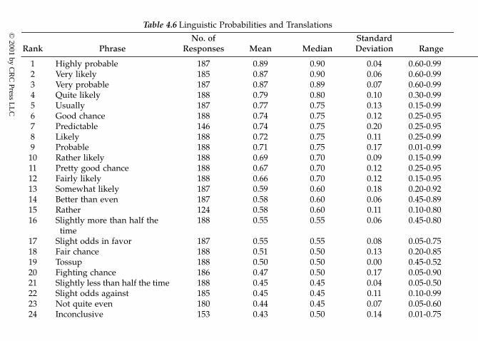
Table 4.6 Linguistic Probabilities and Translations
Rank PhraseNo. of
Responses Mean MedianStandard Deviation Range
1 Highly probable 187 0.89 0.90 0.04 0.60-0.992 Very likely 185 0.87 0.90 0.06 0.60-0.993 Very probable 187 0.87 0.89 0.07 0.60-0.994 Quite likely 188 0.79 0.80 0.10 0.30-0.995 Usually 187 0.77 0.75 0.13 0.15-0.996 Good chance 188 0.74 0.75 0.12 0.25-0.957 Predictable 146 0.74 0.75 0.20 0.25-0.958 Likely 188 0.72 0.75 0.11 0.25-0.999 Probable 188 0.71 0.75 0.17 0.01-0.9910 Rather likely 188 0.69 0.70 0.09 0.15-0.9911 Pretty good chance 188 0.67 0.70 0.12 0.25-0.9512 Fairly likely 188 0.66 0.70 0.12 0.15-0.9513 Somewhat likely 187 0.59 0.60 0.18 0.20-0.9214 Better than even 187 0.58 0.60 0.06 0.45-0.8915 Rather 124 0.58 0.60 0.11 0.10-0.8016 Slightly more than half the
time188 0.55 0.55 0.06 0.45-0.80
17 Slight odds in favor 187 0.55 0.55 0.08 0.05-0.7518 Fair chance 188 0.51 0.50 0.13 0.20-0.8519 Tossup 188 0.50 0.50 0.00 0.45-0.5220 Fighting chance 186 0.47 0.50 0.17 0.05-0.9021 Slightly less than half the time 188 0.45 0.45 0.04 0.05-0.5022 Slight odds against 185 0.45 0.45 0.11 0.10-0.9923 Not quite even 180 0.44 0.45 0.07 0.05-0.6024 Inconclusive 153 0.43 0.50 0.14 0.01-0.75
© 2001 by C
RC
Press LL
C
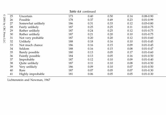
Table 4.6 continued
25 Uncertain 173 0.40 0.50 0.14 0.08-0.9026 Possible 178 0.37 0.49 0.23 0.01-0.9927 Somewhat unlikely 186 0.31 0.33 0.12 0.03-0.8028 Fairly unlikely 187 0.25 0.25 0.11 0.02-0.7529 Rather unlikely 187 0.24 0.25 0.12 0.01-0.7530 Rather unlikely 187 0.21 0.20 0.10 0.01-0.7531 Not very probable 187 0.20 0.20 0.12 0.01-0.6032 Unlikely 188 0.18 0.16 0.10 0.01-0.4533 Not much chance 186 0.16 0.15 0.09 0.01-0.4534 Seldom 188 0.16 0.15 0.08 0.01-0.4735 Barely possible 180 0.13 0.05 0.17 0.01-0.6036 Faintly possible 184 0.13 0.05 0.16 0.01-0.5037 Improbable 187 0.12 0.10 0.09 0.01-0.4038 Quite unlikely 187 0.11 0.10 0.08 0.01-0.5039 Very unlikely 186 0.09 0.10 0.07 0.01-0.5040 Rare 187 0.07 0.05 0.07 0.01-0.3041 Highly improbable 181 0.06 0.05 0.05 0.01-0.30
Lichtenstein and Newman, 1967
© 2001 by C
RC
Press LL
C
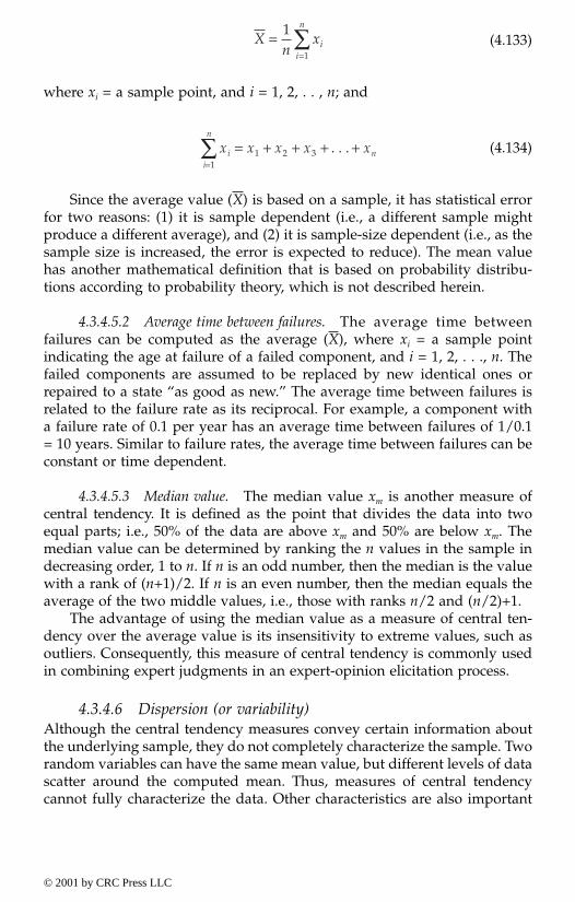
(4.133)
where xi = a sample point, and i = 1, 2, . . , n; and
(4.134)
Since the average value (X) is based on a sample, it has statistical errorfor two reasons: (1) it is sample dependent (i.e., a different sample mightproduce a different average), and (2) it is sample-size dependent (i.e., as thesample size is increased, the error is expected to reduce). The mean valuehas another mathematical definition that is based on probability distribu-tions according to probability theory, which is not described herein.
4.3.4.5.2 Average time between failures. The average time betweenfailures can be computed as the average (X), where xi = a sample pointindicating the age at failure of a failed component, and i = 1, 2, . . ., n. Thefailed components are assumed to be replaced by new identical ones orrepaired to a state “as good as new.” The average time between failures isrelated to the failure rate as its reciprocal. For example, a component witha failure rate of 0.1 per year has an average time between failures of 1/0.1= 10 years. Similar to failure rates, the average time between failures can beconstant or time dependent.
4.3.4.5.3 Median value. The median value xm is another measure ofcentral tendency. It is defined as the point that divides the data into twoequal parts; i.e., 50% of the data are above xm and 50% are below xm. Themedian value can be determined by ranking the n values in the sample indecreasing order, 1 to n. If n is an odd number, then the median is the valuewith a rank of (n+1)/2. If n is an even number, then the median equals theaverage of the two middle values, i.e., those with ranks n/2 and (n/2)+1.
The advantage of using the median value as a measure of central ten-dency over the average value is its insensitivity to extreme values, such asoutliers. Consequently, this measure of central tendency is commonly usedin combining expert judgments in an expert-opinion elicitation process.
4.3.4.6 Dispersion (or variability)Although the central tendency measures convey certain information aboutthe underlying sample, they do not completely characterize the sample. Tworandom variables can have the same mean value, but different levels of datascatter around the computed mean. Thus, measures of central tendencycannot fully characterize the data. Other characteristics are also important
Xn
xii
n
==∑1
1
x x x x xii
n
n=∑ = + + + +
11 2 3 . . .
© 2001 by CRC Press LLC

and necessary. The dispersion measures describe the level of scatter in thedata about the central tendency location.
The most commonly used measure of dispersion is the variance andother quantities that are derived from it, such as the standard deviation andcoefficient of variation. For n observations in a sample that are given equalweight, the variance (S2) is given by
(4.135)
The units of the variance are the square of the units of the variable x;for example, if the variable is measured in pounds per square inch (psi), thevariance has units of (psi)2. Computationally, the variance of a sample canbe determined using the following alternative equation:
(4.136)
By definition, the standard deviation (S) is the square root of the varianceas follows:
(4.137)
It has the same units as both the underlying variable and the centraltendency measures. Therefore, it is a useful descriptor of the dispersion orspread of a sample of data. The coefficient of variation (COV) is a normalizedquantity based on the standard deviation and the mean and is different fromthe covariance. The covariance measures any association between two ran-dom variables. Therefore, the COV is dimensionless and is defined as
(4.138)
It is also used as an expression of the standard deviation in the form ofa percent of the average value. For example, consider X and S to be 50 and20, respectively; therefore, COV(X) = 0.4 or 40%. In this case, the standarddeviation is 40% of the average value.
4.3.4.7 PercentilesA p-percentile value (xp) for a random variable based on a sample is thevalue of the parameter such that p% of the data is less or equal to xp. On the
Sn
x Xii
n2 2
1
11
=− ( )
=∑ –
Sn
xn
xii
n
ii
n2 2
1 1
21
11=
−−
= =
∑ ∑
Sn
xn
xii
n
ii
n
=−
−
= =
∑ ∑11
12
1 1
2
COVSX
=
© 2001 by CRC Press LLC

basis of this definition, the median value is considered to be the 50-percentilevalue.
Aggregating the opinions of experts sometimes requires the computationof the 25, 50, and 75 percentile values. The computation of these valuesdepends on the number of experts providing opinions. Table 4.7 provides asummary of the equations needed for 4 to 20 experts. In the table, Xi meansthe opinion of an expert with the ith smallest value; i.e., X1 ≥ X2 ≥X3 ≥ . . .≥ Xn, where n = number of experts. In the table, the arithmetic average wasused to compute the percentiles. In some cases, where the values of Xi differby power order of magnitude, the geometric average can be used. Expertopinions should not be aggregated in this manner all the times; other aggre-gation methods, as provided in Chapter 5, might be more appropriate andshould be considered.
4.3.4.8 Statistical uncertaintyValues of random variables obtained from sample measurements are com-monly used in making important engineering decisions. For example, sam-ples of river water are collected to estimate the average level of a pollutantin the entire river at that location. Samples of stopping distances are usedto develop a relationship between the speed of a car at the time the brakesare applied and the distance traveled before the car comes to a completehalt. The average of sample measurements of the compressive strength ofconcrete collected during the pouring of a large concrete slab, such as thedeck of a parking garage, is used to help decide whether or not the deck hasthe strength specified in the design specifications. It is important to recognizethe random variables involved in these cases. In each case, the individualmeasurements or samples are values of a random variable, and the computedmean is also the value of a random variable. For example, the transportationengineer measures the stopping distance; each measurement is a samplevalue of the random variable. If ten measurements are made for a car stop-ping from a speed of 50 mph, then the sample consists of ten values of therandom variable. Thus, there are two random variables in this example: thestopping distance and the estimated mean of the stopping distance; this isalso true for the water-quality-pollutant and compressive-strength examples.
The estimated mean for a random variable is considered by itself to bea random variable because different samples about the random variable canproduce different estimated mean values; hence the randomness in the esti-mated mean. When a sample of n measurements of a random variable iscollected, the n values are not necessarily identical. The sample is character-ized by variation. For example, assume that five independent estimates ofthe compressive strength of the concrete in a parking garage deck areobtained from samples of the concrete obtained when the concrete waspoured. For illustration purposes, assume that the five compressive strengthmeasurements are 3250, 3610, 3460, 3380, and 3510 psi. These measurementsproduce a mean of 3442 psi and a standard deviation of 135.9 psi. Assumethat another sample of five measurements of concrete strength is obtained
© 2001 by CRC Press LLC
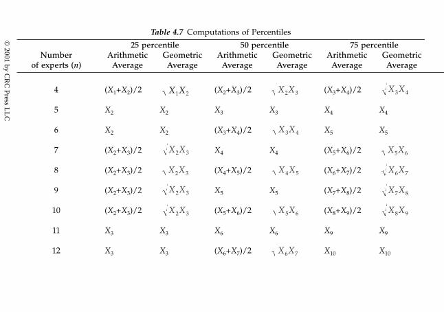
Table 4.7 Computations of Percentiles
Numberof experts (n)
25 percentile 50 percentile 75 percentileArithmetic
AverageGeometric
AverageArithmetic
AverageGeometric
AverageArithmetic
AverageGeometric
Average
4 (X1+X2)/2 (X2+X3)/2 (X3+X4)/2
5 X2 X2 X3 X3 X4 X4
6 X2 X2 (X3+X4)/2 X5 X5
7 (X2+X3)/2 X4 X4 (X5+X6)/2
8 (X2+X3)/2 (X4+X5)/2 (X6+X7)/2
9 (X2+X3)/2 X5 X5 (X7+X8)/2
10 (X2+X3)/2 (X5+X6)/2 (X8+X9)/2
11 X3 X3 X6 X6 X9 X9
12 X3 X3 (X6+X7)/2 X10 X10
X X1 2 X X2 3 X X3 4
X X3 4
X X2 3 X X5 6
X X2 3 X X4 5 X X6 7
X X2 3 X X7 8
X X2 3 X X5 6 X X8 9
X X6 7
© 2001 by C
RC
Press LL
C

Table 4.7 continued
13 (X3+X4)/2 X7 X7 (X10+X11)/2
14 (X3+X4)/2 (X7+X8)/2 (X11+X12)/2
15 X4 X4 X8 X8 X12 X12
16 X4 X4 (X8+X9)/2 X13 X13
17 (X4+X5)/2 X9 X9 (X13+X14)/2
18 (X4+X5)/2 (X9+X10)/2 (X14+X15)/2
19 X5 X5 X10 X10 X15 X15
20 X5 X5 (X10+X11)/2 X15 X15
X X3 4 X X10 11
X X3 4 X X7 8 X X11 12
X X8 9
X X4 5 X X13 14
X X4 5 X X9 10 X X14 15
X X10 11
© 2001 by C
RC
Press LL
C

from the same concrete pour; however, the values are 3650, 3360, 3328, 3420,and 3260 psi. In this case, the estimated mean and standard deviation are3404, and 149.3 psi, respectively. Therefore, the individual measurement andthe mean are values of two different random variables, i.e., X and X.
It would greatly simplify decision making if the sample measurementswere identical, i.e., if there were no sampling variation so the standarddeviation would be zero. Unfortunately, that is never the case, so decisionsmust be made in the presence of uncertainty. For example, assume in theparking garage example that the building code requires a mean compressivestrength of 3500 psi. Since the mean of 3442 psi based on the first sample isless than the required 3500 psi, should we conclude that the garage deckdoes not meet the design specifications? Unfortunately, decision making isnot that simple. If a third sample of five measurements is randomly collectedfrom other locations on the garage deck, the collected values are just as likelyto be: 3720, 3440, 3590, 3270, and 3610 psi. This sample of five produces amean of 3526 psi and a standard deviation of 174.4 psi. In this case, the meanexceeds the design standard of 3500 psi. Since the sample mean is greaterthan the specified value of 3500 psi, can we conclude that the concrete is ofadequate strength? Unfortunately, we cannot conclude with certainty thatthe strength is adequate any more than we could conclude with the firstsample that the strength was inadequate. The fact that different samples leadto different means is an indication that we cannot conclude that the designspecification is not met just because the sample mean is less than the designstandard. We need to have more assurance.
The data that are collected on some variable or parameter representsample information, but it is not complete by itself, and predictions are notmade directly from the sample. The intermediate step between samplingand prediction is the identification of the underlying population. The sampleis used to identify the population, and then the population is used to makepredictions or decisions. This sample-to-population-to-prediction sequenceis true for the univariate methods in statistics.
The need, then, is for a systematic decision process that takes intoaccount the variation that can be expected from one sample to another. Thedecision process must also be able to reflect the risk of making an incorrectdecision. This decision making can be made using statistical methods, forexample, hypothesis testing as described by Ayyub and McCuen (1997).
4.3.4.9 Bayesian methodsEngineers commonly need to solve a problem and make decisions based onlimited information about one or more of the parameters of the problem.The types of information available to them can be classified using commonlyused terminology in the Bayesian literature as follows:
• objective or empirical information based on experimental results, orobservations; and
© 2001 by CRC Press LLC

• subjective information based on experience, intuition, other previousproblems that are similar to the one under consideration, or thephysics of the problem.
The first type of information can be dealt with using the theories ofprobability and statistics as described in previous chapters. In this type,probability is interpreted as the frequency of occurrence assuming sufficientrepetitions of the problem, its outcomes, and parameters, as a basis of theinformation. The second type of information is subjective and can dependon the engineer or analyst studying the problem. In this type, uncertaintythat exists needs to be dealt with using probabilities. However, the definitionof probability is not the same as the first type because it is viewed herein asa subjective probability that reflects the state of knowledge of the engineeror the analyst.
4.3.4.9.1 Bayesian probabilities. It is common in engineering toencounter problems with both objective and subjective types of information.In these cases, it is desirable to utilize both types of information to obtainsolutions or make decisions. The subjective probabilities are assumed toconstitute a prior knowledge about a parameter, with gained objective infor-mation (or probabilities). Combining the two types produces posteriorknowledge. The combination is performed based on Bayes’ theoremas described by Ayyub and McCuen (1997). If A1, A2, . . ., An represent theprior (subjective) information, or a partition of a sample space S, and E ⊂ Srepresents the objective information (or arbitrary event) as shown inFigure 4.16, the theorem of total probability states that
P(E) = P(A1) P(E|A1) + P(A2) P(E|A2) + . . . + P(An) P(E|An) (4.139)
where P(Ai) the probability of the event Ai, and E|Ai the occurrence ofE given Ai, for i = 1, 2, . . ., n. This theorem is very important in computingthe probability of the event E, especially in practical cases when the proba-bility cannot be computed directly, but the probabilities of the partitioningevents and the conditional probabilities can be computed.
Bayes’ theorem is based on the same conditions of partitioning andevents as the theorem of total probability and is very useful in computingthe posterior (or reverse) probability of the type P(Ai|E), for i = 1, 2, . . ., n.The posterior probability can be computed as follows:
(4.140)
The denominator of this equation is P(E), which is based on the theoremof total probability. According to Equation 4.139, the prior knowledge, P(Ai),
P A EP A P E A
P A P E A P A P E A P A P E Ai
i i
n n
( ) =( ) ( )
( ) ( ) + ( ) ( ) + + ( ) ( )1 1 2 2 . . .
© 2001 by CRC Press LLC
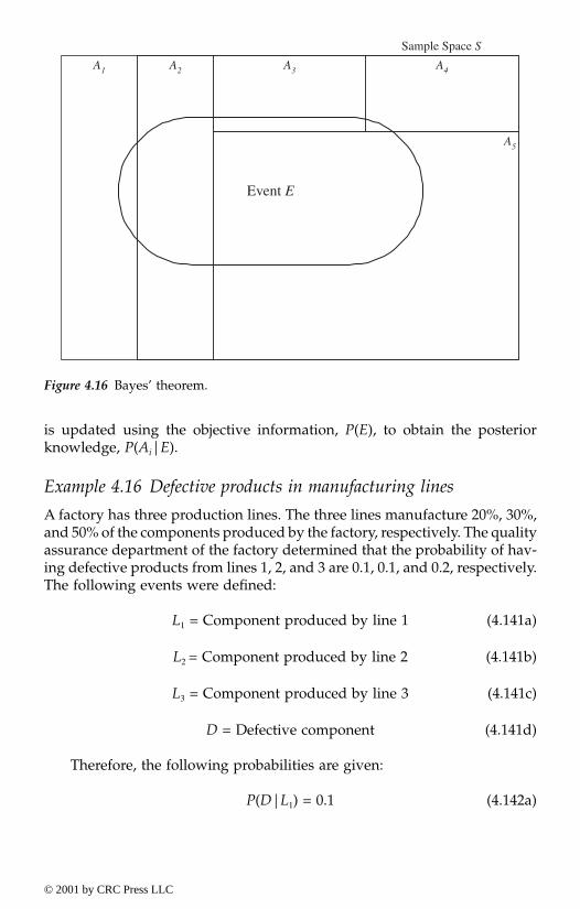
is updated using the objective information, P(E), to obtain the posteriorknowledge, P(Ai|E).
Example 4.16 Defective products in manufacturing lines
A factory has three production lines. The three lines manufacture 20%, 30%,and 50% of the components produced by the factory, respectively. The qualityassurance department of the factory determined that the probability of hav-ing defective products from lines 1, 2, and 3 are 0.1, 0.1, and 0.2, respectively.The following events were defined:
L1 = Component produced by line 1 (4.141a)
L2 = Component produced by line 2 (4.141b)
L3 = Component produced by line 3 (4.141c)
D = Defective component (4.141d)
Therefore, the following probabilities are given:
P(D|L1) = 0.1 (4.142a)
Figure 4.16 Bayes’ theorem.
A1 A2 A3 A4
A5
Event E
Sample Space S
© 2001 by CRC Press LLC
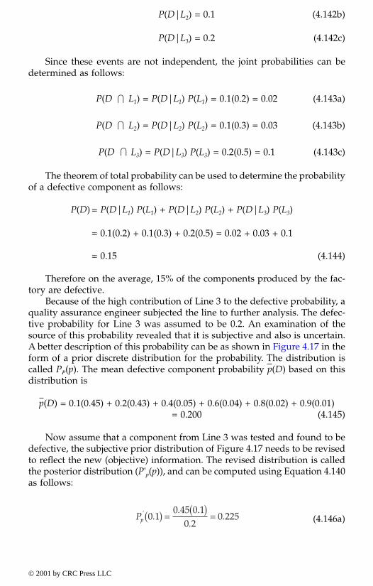
P(D|L2) = 0.1 (4.142b)
P(D|L3) = 0.2 (4.142c)
Since these events are not independent, the joint probabilities can bedetermined as follows:
P(D L1) = P(D|L1) P(L1) = 0.1(0.2) = 0.02 (4.143a)
P(D L2) = P(D|L2) P(L2) = 0.1(0.3) = 0.03 (4.143b)
P(D L3) = P(D|L3) P(L3) = 0.2(0.5) = 0.1 (4.143c)
The theorem of total probability can be used to determine the probabilityof a defective component as follows:
P(D) = P(D|L1) P(L1) + P(D|L2) P(L2) + P(D|L3) P(L3)
= 0.1(0.2) + 0.1(0.3) + 0.2(0.5) = 0.02 + 0.03 + 0.1
= 0.15 (4.144)
Therefore on the average, 15% of the components produced by the fac-tory are defective.
Because of the high contribution of Line 3 to the defective probability, aquality assurance engineer subjected the line to further analysis. The defec-tive probability for Line 3 was assumed to be 0.2. An examination of thesource of this probability revealed that it is subjective and also is uncertain.A better description of this probability can be as shown in Figure 4.17 in theform of a prior discrete distribution for the probability. The distribution iscalled PP(p). The mean defective component probability p(D) based on thisdistribution is
p(D) = 0.1(0.45) + 0.2(0.43) + 0.4(0.05) + 0.6(0.04) + 0.8(0.02) + 0.9(0.01)= 0.200 (4.145)
Now assume that a component from Line 3 was tested and found to bedefective, the subjective prior distribution of Figure 4.17 needs to be revisedto reflect the new (objective) information. The revised distribution is calledthe posterior distribution (P'p(p)), and can be computed using Equation 4.140as follows:
(4.146a)
I
I
I
Pp' .
. ..
.0 10 45 0 1
0 20 225( ) = ( ) =
© 2001 by CRC Press LLC

Similarly, the following posterior probabilities can be computed:
(4.146b)
(4.146c)
(4.146d)
(4.146e)
(4.146f)
The resulting probabilities in Equations 4.146 add up to 1. Also, theaverage probability of 0.2 can be viewed as a normalizing factor for com-puting these probabilities. The mean defective component probability p(D)based on the posterior distribution is
p(D) = 0.1(0.225) + 0.2(0.430) + 0.4(0.100) + 0.6(0.120)+ 0.8(0.080) + 0.9(0.045) = 0.325 (4.147)
Figure 4.17 Prior probability distribution for defective probability of line 3.
0.45 0.43
0.05 0.04 0.02 0.010
0.1
0.2
0.3
0.4
0.5
0.1 0.2 0.4 0.6 0.8 0.9
Defective Probability, p
Prio
r Pr
obab
ility
, PP(p
)
Pp' .
. ..
.0 20 43 0 2
0 20 430( ) = ( ) =
Pp' .
. ..
.0 40 05 0 4
0 20 100( ) = ( ) =
Pp' .
. ..
.0 60 04 0 6
0 20 120( ) = ( ) =
Pp' .
. ..
.0 80 02 0 8
0 20 08( ) = ( ) =
Pp' .
. ..
.0 90 01 0 9
0 20 045( ) = ( ) =
© 2001 by CRC Press LLC
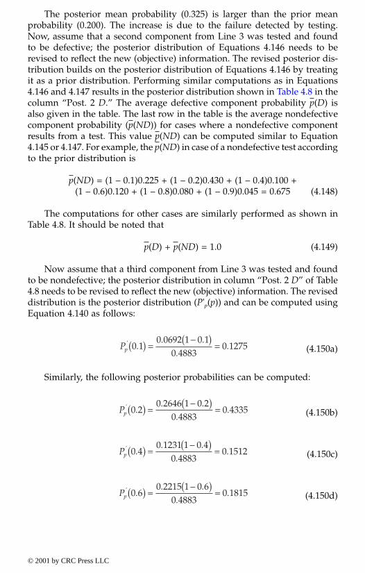
The posterior mean probability (0.325) is larger than the prior meanprobability (0.200). The increase is due to the failure detected by testing.Now, assume that a second component from Line 3 was tested and foundto be defective; the posterior distribution of Equations 4.146 needs to berevised to reflect the new (objective) information. The revised posterior dis-tribution builds on the posterior distribution of Equations 4.146 by treatingit as a prior distribution. Performing similar computations as in Equations4.146 and 4.147 results in the posterior distribution shown in Table 4.8 in thecolumn “Post. 2 D.” The average defective component probability p(D) isalso given in the table. The last row in the table is the average nondefectivecomponent probability (p(ND)) for cases where a nondefective componentresults from a test. This value p(ND) can be computed similar to Equation4.145 or 4.147. For example, the p(ND) in case of a nondefective test accordingto the prior distribution is
p(ND) = (1 – 0.1)0.225 + (1 – 0.2)0.430 + (1 – 0.4)0.100 +(1 – 0.6)0.120 + (1 – 0.8)0.080 + (1 – 0.9)0.045 = 0.675 (4.148)
The computations for other cases are similarly performed as shown inTable 4.8. It should be noted that
p(D) + p(ND) = 1.0 (4.149)
Now assume that a third component from Line 3 was tested and foundto be nondefective; the posterior distribution in column “Post. 2 D” of Table4.8 needs to be revised to reflect the new (objective) information. The reviseddistribution is the posterior distribution (P'p(p)) and can be computed usingEquation 4.140 as follows:
(4.150a)
Similarly, the following posterior probabilities can be computed:
(4.150b)
(4.150c)
(4.150d)
Pp' .
. ..
.0 10 0692 1 0 1
0 48830 1275( ) =
−( ) =
Pp' .
. ..
.0 20 2646 1 0 2
0 48830 4335( ) =
−( ) =
Pp' .
. ..
.0 40 1231 1 0 4
0 48830 1512( ) =
−( ) =
Pp' .
. ..
.0 60 2215 1 0 6
0 48830 1815( ) =
−( ) =
© 2001 by CRC Press LLC

Table 4.8 Prior and Posterior Distributions for Line 3
Probability, p P(p) Post. 1 D Post. 2 D Post. 3 ND Post. 4 D Post. 5 D Post. 6 D Post. 7 D Post. 8 D Post. 9 D Post. 10 D
0.1 0.45 0.225 0.0692308 0.127599244 0.035809 0.0070718 0.0011355 0.0001638 2.22693E-05 2.912E-06 3.703E-07
0.2 0.43 0.43 0.2646154 0.433522369 0.2433245 0.0961062 0.0308633 0.0089068 0.002421135 0.0006332 0.0001611
0.4 0.05 0.1 0.1230769 0.151228733 0.1697613 0.1341016 0.08613 0.0497125 0.027026626 0.0141359 0.0071914
0.6 0.04 0.12 0.2215385 0.18147448 0.3055703 0.3620744 0.3488266 0.3020033 0.246280127 0.1932203 0.1474458
0.8 0.02 0.08 0.1969231 0.080655325 0.1810787 0.2860835 0.3674882 0.4242131 0.461254413 0.482506 0.4909318
0.9 0.01 0.045 0.1246154 0.025519849 0.0644562 0.1145626 0.1655564 0.2150004 0.262995429 0.3095016 0.3542696
p(D) 0.2 0.325 0.5116923 0.356332703 0.506366 0.6227868 0.6930255 0.7357556 0.764764597 0.7862698 0.8029643
p(ND) 0.8 0.675 0.4883077 0.643667297 0.493634 0.3772132 0.3069745 0.2642444 0.235235403 0.2137302 0.1970357
© 2001 by C
RC
Press LL
C

(4.150e)
(4.150f)
The resulting probabilities in Equations 4.150 add up to 1. The proba-bility p(ND) of 0.4883 was used in these calculations. The results of thesecalculations and the mean probability p(D) are shown in Table 4.8. It can benoted from the table that the mean defective component probabilitydecreases as nondefective components are obtained through testing.
If the next sevenstests result in defective components, the resulting pos-terior distributions are shown in Table 4.8. The results are also shown inFigure 4.18. It can be observed from the figure that the average probabilityis approaching 1 as more and more defective tests are obtained. Also, theeffect of a nondefective component on the posterior probabilities can be seenin this figure.
4.3.4.10 Interval probabilitiesThe term interval probabilities has more than one meaning as reported byMoore (1979), Dempster (1976a, 1976b), Cui and Blockley (1990), and Fersonet al. (1999). Various models for dealing with interval probabilities are pro-vided in subsequent sections, but this section summarizes the model sug-gested by Cui and Blockley (1990), who introduced interval probabilitiesbased on probability axioms maintaining the additive condition of
Figure 4.18 Posterior distributions for line 3.
0
0.1
0.2
0.3
0.4
0.5
0.6
0.7
0.8
0.9
0 1 2 3 4 5 6 7 8 9 10
Test Number
Post
erio
r Pr
obab
ility
0.1 0.2 0.4 0.6 0.8 0.9 Average D Probability Average ND Probability
Pp' .
. ..
.0 80 1969 1 0 8
0 48830 0807( ) =
−( ) =
Pp' .
. ..
.0 90 12461 1 0 9
0 48830 0255( ) =
−( ) =
© 2001 by CRC Press LLC
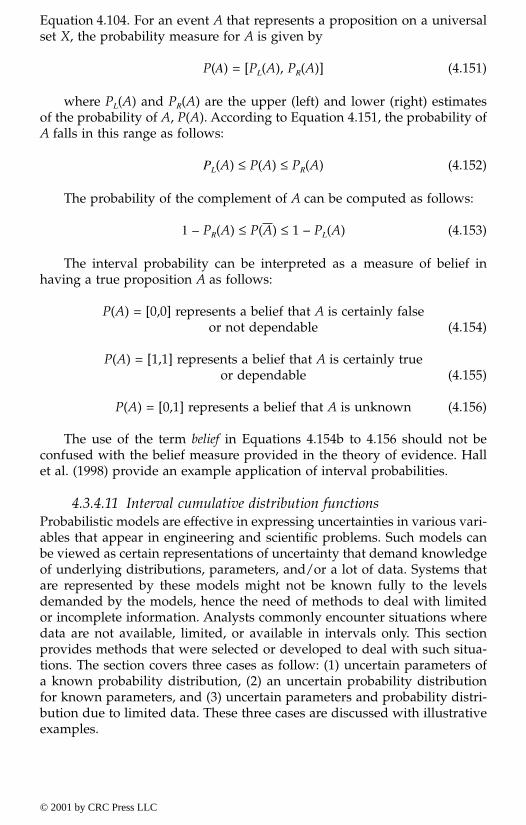
Equation 4.104. For an event A that represents a proposition on a universalset X, the probability measure for A is given by
P(A) = [PL(A), PR(A)] (4.151)
where PL(A) and PR(A) are the upper (left) and lower (right) estimatesof the probability of A, P(A). According to Equation 4.151, the probability ofA falls in this range as follows:
PL(A) ≤ P(A) ≤ PR(A) (4.152)
The probability of the complement of A can be computed as follows:
1 – PR(A) ≤ P(A) ≤ 1 – PL(A) (4.153)
The interval probability can be interpreted as a measure of belief inhaving a true proposition A as follows:
P(A) = [0,0] represents a belief that A is certainly falseor not dependable (4.154)
P(A) = [1,1] represents a belief that A is certainly trueor dependable (4.155)
P(A) = [0,1] represents a belief that A is unknown (4.156)
The use of the term belief in Equations 4.154b to 4.156 should not beconfused with the belief measure provided in the theory of evidence. Hallet al. (1998) provide an example application of interval probabilities.
4.3.4.11 Interval cumulative distribution functionsProbabilistic models are effective in expressing uncertainties in various vari-ables that appear in engineering and scientific problems. Such models canbe viewed as certain representations of uncertainty that demand knowledgeof underlying distributions, parameters, and/or a lot of data. Systems thatare represented by these models might not be known fully to the levelsdemanded by the models, hence the need of methods to deal with limitedor incomplete information. Analysts commonly encounter situations wheredata are not available, limited, or available in intervals only. This sectionprovides methods that were selected or developed to deal with such situa-tions. The section covers three cases as follow: (1) uncertain parameters ofa known probability distribution, (2) an uncertain probability distributionfor known parameters, and (3) uncertain parameters and probability distri-bution due to limited data. These three cases are discussed with illustrativeexamples.
© 2001 by CRC Press LLC
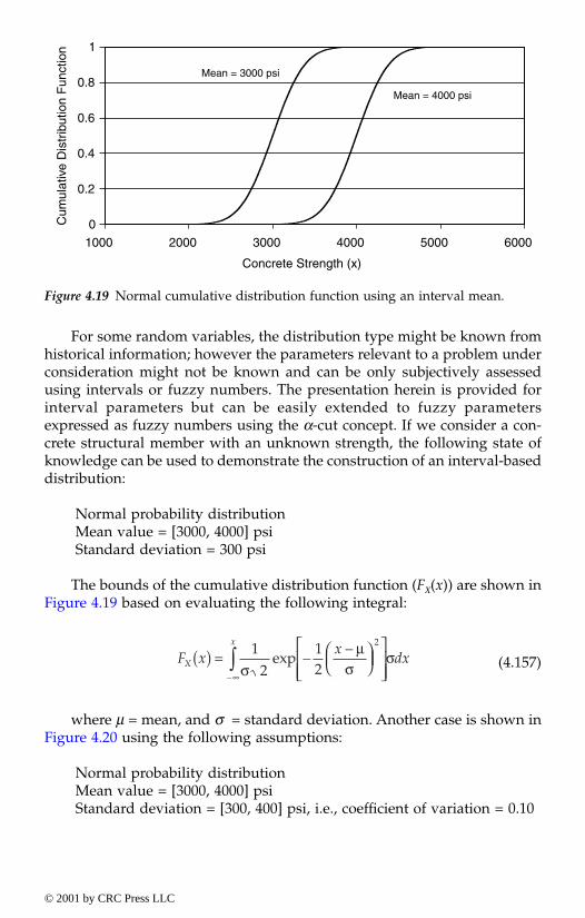
For some random variables, the distribution type might be known fromhistorical information; however the parameters relevant to a problem underconsideration might not be known and can be only subjectively assessedusing intervals or fuzzy numbers. The presentation herein is provided forinterval parameters but can be easily extended to fuzzy parametersexpressed as fuzzy numbers using the α-cut concept. If we consider a con-crete structural member with an unknown strength, the following state ofknowledge can be used to demonstrate the construction of an interval-baseddistribution:
Normal probability distributionMean value = [3000, 4000] psiStandard deviation = 300 psi
The bounds of the cumulative distribution function (FX(x)) are shown inFigure 4.19 based on evaluating the following integral:
(4.157)
where µ = mean, and σ = standard deviation. Another case is shown inFigure 4.20 using the following assumptions:
Normal probability distributionMean value = [3000, 4000] psiStandard deviation = [300, 400] psi, i.e., coefficient of variation = 0.10
Figure 4.19 Normal cumulative distribution function using an interval mean.
0
0.2
0.4
0.6
0.8
1
1000 2000 3000 4000 5000 6000
Concrete Strength (x)
Cum
ulat
ive
Dis
trib
utio
n F
unct
ion
Mean = 3000 psi
Mean = 4000 psi
F xx
dxX
x
( ) =
∞
∫ 12
12
2
σµ
σσexp –
–
–
© 2001 by CRC Press LLC
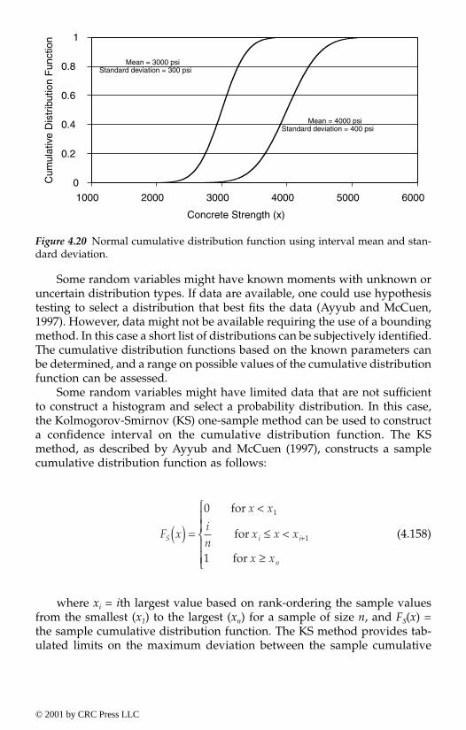
Some random variables might have known moments with unknown oruncertain distribution types. If data are available, one could use hypothesistesting to select a distribution that best fits the data (Ayyub and McCuen,1997). However, data might not be available requiring the use of a boundingmethod. In this case a short list of distributions can be subjectively identified.The cumulative distribution functions based on the known parameters canbe determined, and a range on possible values of the cumulative distributionfunction can be assessed.
Some random variables might have limited data that are not sufficientto construct a histogram and select a probability distribution. In this case,the Kolmogorov-Smirnov (KS) one-sample method can be used to constructa confidence interval on the cumulative distribution function. The KSmethod, as described by Ayyub and McCuen (1997), constructs a samplecumulative distribution function as follows:
(4.158)
where xi = ith largest value based on rank-ordering the sample valuesfrom the smallest (x1) to the largest (xn) for a sample of size n, and FS(x) =the sample cumulative distribution function. The KS method provides tab-ulated limits on the maximum deviation between the sample cumulative
Figure 4.20 Normal cumulative distribution function using interval mean and stan-dard deviation.
0
0.2
0.4
0.6
0.8
1
1000 2000 3000 4000 5000 6000
Concrete Strength (x)
Cum
ulat
ive
Dis
trib
utio
n F
unct
ion
Mean = 3000 psiStandard deviation = 300 psi
Mean = 4000 psiStandard deviation = 400 psi
F x
x x
in
x x x
x x
S i i
n
( ) =
<
≤ <
≥
+
0
1
1
1
for
for
for
© 2001 by CRC Press LLC
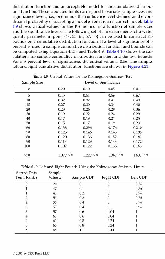
distribution function and an acceptable model for the cumulative distribu-tion function. These tabulated limits correspond to various sample sizes andsignificance levels, i.e., one minus the confidence level defined as the con-ditional probability of accepting a model given it is an incorrect model. Table4.9 shows critical values for the KS method as a function of sample sizesand the significance levels. The following set of 5 measurements of a waterquality parameter in ppm: {47, 53, 61, 57, 65} can be used to construct KSbounds on a cumulative distribution function. If a level of significance of 5percent is used, a sample cumulative distribution function and bounds canbe computed using Equation 4.158 and Table 4.9. Table 4.10 shows the cal-culations for sample cumulative distribution function and the two bounds.For a 5 percent level of significance, the critical value is 0.56. The sample,left and right cumulative distribution functions are shown in Figure 4.21.
Table 4.9 Critical Values for the Kolmogorov-Smirnov Test
Sample Size Level of Significance
n 0.20 0.10 0.05 0.01
5 0.45 0.51 0.56 0.6710 0.32 0.37 0.41 0.4915 0.27 0.30 0.34 0.4020 0.23 0.26 0.29 0.3630 0.19 0.22 0.24 0.2940 0.17 0.19 0.21 0.2550 0.15 0.17 0.19 0.2360 0.138 0.296 0.176 0.21070 0.125 0.146 0.163 0.19580 0.120 0.136 0.152 0.18290 0.113 0.129 0.143 0.172
100 0.107 0.122 0.136 0.163
>50 1.07/ 1.22/ 1.36/ 1.63/
Table 4.10 Left and Right Bounds Using the Kolmogorov-Smirnov Limits
Sorted Data Point Rank i
SampleValue x Sample CDF Right CDF Left CDF
0 20 0 0 0.561 47 0 0 0.561 47 0.2 0 0.762 53 0.2 0 0.762 53 0.4 0 0.963 57 0.4 0 0.963 57 0.6 0.04 14 61 0.6 0.04 14 61 0.8 0.24 15 65 0.8 0.24 15 65 1 0.44 1
n n n n
© 2001 by CRC Press LLC
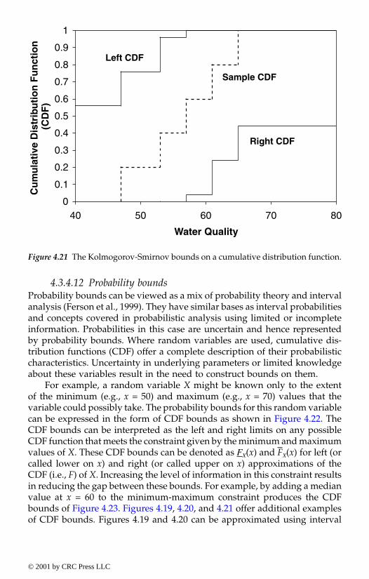
4.3.4.12 Probability boundsProbability bounds can be viewed as a mix of probability theory and intervalanalysis (Ferson et al., 1999). They have similar bases as interval probabilitiesand concepts covered in probabilistic analysis using limited or incompleteinformation. Probabilities in this case are uncertain and hence representedby probability bounds. Where random variables are used, cumulative dis-tribution functions (CDF) offer a complete description of their probabilisticcharacteristics. Uncertainty in underlying parameters or limited knowledgeabout these variables result in the need to construct bounds on them.
For example, a random variable X might be known only to the extentof the minimum (e.g., x = 50) and maximum (e.g., x = 70) values that thevariable could possibly take. The probability bounds for this random variablecan be expressed in the form of CDF bounds as shown in Figure 4.22. TheCDF bounds can be interpreted as the left and right limits on any possibleCDF function that meets the constraint given by the minimum and maximumvalues of X. These CDF bounds can be denoted as FX(x) and FX(x) for left (orcalled lower on x) and right (or called upper on x) approximations of theCDF (i.e., F) of X. Increasing the level of information in this constraint resultsin reducing the gap between these bounds. For example, by adding a medianvalue at x = 60 to the minimum-maximum constraint produces the CDFbounds of Figure 4.23. Figures 4.19, 4.20, and 4.21 offer additional examplesof CDF bounds. Figures 4.19 and 4.20 can be approximated using interval
Figure 4.21 The Kolmogorov-Smirnov bounds on a cumulative distribution function.
0
0.1
0.2
0.3
0.4
0.5
0.6
0.7
0.8
0.9
1
40 50 60 70 80
Water Quality
Cu
mu
lati
ve D
istr
ibu
tio
n F
un
ctio
n
(CD
F)
Sample CDF
Left CDF
Right CDF
© 2001 by CRC Press LLC
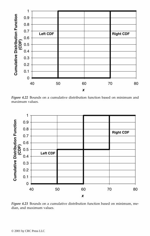
Figure 4.22 Bounds on a cumulative distribution function based on minimum andmaximum values.
Figure 4.23 Bounds on a cumulative distribution function based on minimum, me-dian, and maximum values.
0
0.1
0.2
0.3
0.4
0.5
0.6
0.7
0.8
0.9
1
40 50 60 70 80
x
Cu
mu
lati
ve D
istr
ibu
tio
n F
un
ctio
n
(CD
F)
Right CDFLeft CDF
0
0.1
0.2
0.3
0.4
0.5
0.6
0.7
0.8
0.9
1
40 50 60 70 80
x
Cu
mu
lati
ve D
istr
ibu
tio
n F
un
ctio
n
(CD
F)
Right CDF
Left CDF
© 2001 by CRC Press LLC
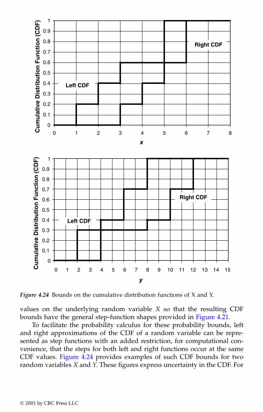
values on the underlying random variable X so that the resulting CDFbounds have the general step-function shapes provided in Figure 4.21.
To facilitate the probability calculus for these probability bounds, leftand right approximations of the CDF of a random variable can be repre-sented as step functions with an added restriction, for computational con-venience, that the steps for both left and right functions occur at the sameCDF values. Figure 4.24 provides examples of such CDF bounds for tworandom variables X and Y. These figures express uncertainty in the CDF. For
Figure 4.24 Bounds on the cumulative distribution functions of X and Y.
0
0.1
0.2
0.3
0.4
0.5
0.6
0.7
0.8
0.9
1
0 1 2 3 4 5 6 7 8
x
Cu
mu
lati
ve D
istr
ibu
tio
n F
un
ctio
n (
CD
F)
Right CDF
Left CDF
0
0.1
0.2
0.3
0.4
0.5
0.6
0.7
0.8
0.9
1
0 1 2 3 4 5 6 7 8 9 10 11 12 13 14 15
y
Cu
mu
lati
ve D
istr
ibu
tio
n F
un
ctio
n (
CD
F)
Right CDF
Left CDF
© 2001 by CRC Press LLC

example, Figure 4.24 provides the CDF bounds at x = 3.5 of [0.2, 0.6]. Also,the same figure expresses the uncertainty in the value of X at a given CDFvalue. For a CDF value (percentile value) of 0.90, the value of x belongs tothe interval [5, 6].
Random variables defined by CDF bounds can be combined using arith-metic operations such as addition, subtraction, multiplication, and division;however information on underlying dependencies between the two randomvariables is needed in order to assess the combined result. Two cases areconsidered in this section as follows: (1) the case of an underlying indepen-dence between two random variables such as X and Y, and (2) the case ofunderlying, but unknown, dependencies between two random variablessuch as X and Y.
The underlying independence assumption for X and Y allows for com-puting, for example X + Y, by portioning the spaces of X and Y to convenientintervals, performing interval arithmetic on all the combinations of the Car-tesian-space of X and Y, and computing the corresponding probabilities ofthe resulting intervals as the product of the respective pairs. The computa-tional procedure is demonstrated using the random variable X and Y ofFigure 4.24 to evaluate their addition, i.e., X+Y as shown in Table 4.11. Theleft and right probability bounds of the CDF of the addition result Z can beevaluated as shown in Table 4.12. Table 4.12 was constructed by identifyingthe range of Z from Table 4.11, from 3 to 18 in general increments of one.Then for each Z value, such as z, the left bound was constructed as thecumulative sum of all interval probabilities for Z in Table 4.11 where thelower (left) limits of the intervals are less or equal to z. The right bound forZ can be constructed in a similar manner as the cumulative sum of intervalprobabilities from Table 4.11 where the upper (right) values of the intervalsare less or equal to z. The resulting probability bounds of Z = X + Y areshown in Figure 4.25. Other arithmetic operations such as subtraction, mul-tiplication, and division can be performed in a similar manner to the aboveprocess for addition.
The case of an underlying, but unknown, dependency between tworandom variables such as X and Y requires arithmetic operations on X andY to be conducted using a probability-bound convolution with the constraintthat the sum of probabilities must be one. Frank et al. (1987), Nelson (1999),and Williamson and Downs (1990) provided the following probabilitybounds on Z = X * Y, where * ∈ [+,–,×,÷], for arithmetic operations withunknown dependencies between two random variables such as X and Y:
(4.159)
(4.160)
F z F u F vX Yz u v
X Y+ ( ) = ( ) + ( )[ ]{ }max maxsuch that = +
– ,1 0
F z F u F vX Y z u v X Y+ ( ) = ( ) + ( )[ ]{ }min minsuch that = +
,1
© 2001 by CRC Press LLC
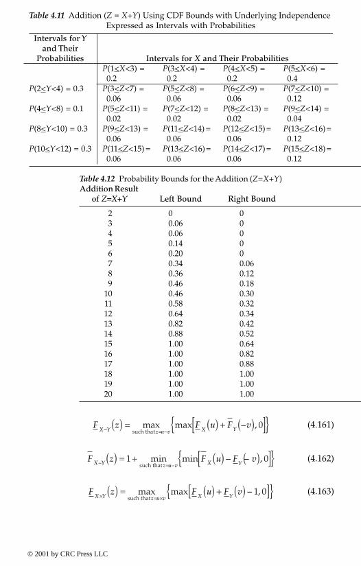
(4.161)
(4.162)
(4.163)
Table 4.11 Addition (Z = X+Y) Using CDF Bounds with Underlying Independence Expressed as Intervals with Probabilities
Intervals for Yand Their
Probabilities Intervals for X and Their ProbabilitiesP(1<X<3) =
0.2P(3<X<4) =
0.2P(4<X<5) =
0.2P(5<X<6) =
0.4P(2<Y<4) = 0.3 P(3<Z<7) =
0.06P(5<Z<8) =
0.06P(6<Z<9) =
0.06P(7<Z<10) =
0.12P(4<Y<8) = 0.1 P(5<Z<11) =
0.02P(7<Z<12) =
0.02P(8<Z<13) =
0.02P(9<Z<14) =
0.04P(8<Y<10) = 0.3 P(9<Z<13) =
0.06P(11<Z<14) =
0.06P(12<Z<15) = 0.06
P(13<Z<16) = 0.12
P(10<Y<12) = 0.3 P(11<Z<15) = 0.06
P(13<Z<16) = 0.06
P(14<Z<17) = 0.06
P(15<Z<18) = 0.12
Table 4.12 Probability Bounds for the Addition (Z=X+Y)Addition Result
of Z=X+Y Left Bound Right Bound
2 0 03 0.06 04 0.06 05 0.14 06 0.20 07 0.34 0.068 0.36 0.129 0.46 0.18
10 0.46 0.3011 0.58 0.3212 0.64 0.3413 0.82 0.4214 0.88 0.5215 1.00 0.6416 1.00 0.8217 1.00 0.8818 1.00 1.0019 1.00 1.0020 1.00 1.00
F z F u F vX Y z u v X Y–
– ,( ) = ( ) + ( )[ ]{ }max maxsuch that = –
0
F z F u F vX Y z u v X Y– – – ,( ) = + ( ) ( )[ ]{ }1 0min minsuch that = –
F z F u F vX Y z u v X Y× ×
( ) = ( ) + ( )[ ]{ }max maxsuch that =
– ,1 0
© 2001 by CRC Press LLC

(4.164)
(4.165)
(4.166)
Williamson and Downs (1990) showed that the above bounds hold forthe arithmetic operation of addition and multiplication for both positiveand negative X and Y, and for the arithmetic operation of subtraction anddivision for only positive X and Y. Regan et al. (2000) generalized Equations4.159 to 4.166 to any arithmetic operation regardless of the sign of X and Yby using the interval mathematics of Equations 4.37 to 4.40 that, in the case
Figure 4.25 Bounds on the cumulative distribution functions of Z = X + Y.
0
0.1
0.2
0.3
0.4
0.5
0.6
0.7
0.8
0.9
1
2 3 4 5 6 7 8 9 1011121314151617181920
z
Cu
mu
lati
ve D
istr
ibu
tio
n F
un
ctio
n
(CD
F) Right CDF
Left CDF
F z F u F vX Y z u v X Y× ×( ) = ( ) + ( )[ ]{ }min min
such that =,1
F z F u F vX Y z u v X Y÷ ÷
( ) = ( ) ( )[ ]{ }max maxsuch that =
– / ,1 0
F z F u F vX Y z u v X Y÷ ÷
( ) = + ( ) ( )[ ]{ }1 1 0min minsuch that =
– / ,
© 2001 by CRC Press LLC

of subtraction and division, combines the lower bound of one variable withthe upper bound of another and vise versa as required by these equations.For two events A and B with given probabilities P(A) and P(B), the limitsprovided by Equations 4.159 to 4.166 are partially based on the conjunctionand disjunction, called Frechet, inequalities as follow, respectively:
Conjunction: max(0, P(A) + P(B) – 1) ≤ P(A ∩ B) ≤min(P(A),P(B)) (4.167)
Disjunction: max(P(A),P(B)) ≤ P(A ∪ B) ≤min(1, P(A) + P(B)) (4.168)
Equations 4.167 and 4.168 usually result in wide limits, and their use forCDF functions can violate the constraint that the sum of probabilities mustbe one, whereas Equations 4.159 to 4.166 do not violate this constraint.
Regan et al. (2000) showed the equivalency of Equations 4.159 to 4.166in propagating uncertainty to methods offered by Walley (1991) for impreciseprobabilities, and Dempster-Shafer belief functions as provided by Yager(1986).
4.3.5 Possibility theory
Possibility theory and its monotone measures of necessity and possibilityare based on crisp sets and the nonadditive properties of Equations 4.103and 4.105 as described by Klir and Folger (1988), Klir and Wierman (1999),Dubois and Prade (1988), and De Cooman (1997). The possibility theory isa special case of the Dempster-Shafer theory of evidence and its monotonemeasures of belief and plausibility by requiring the underlying subsets of auniverse X to be nested, i.e., A1 ⊂ A2 ⊂ . . . ⊂ X. Nested subsets on X arecalled chains. Nested subsets for an evidence body result in minimal conflictswith each other; therefore, their belief and plausibility measures, callednecessity and possibility measures respectively, in this case, are described tobe consonant. An example of five nested sets (Ai) with 10 discrete elements(xj) is shown in Figure 4.26. For nested subsets, the associated belief andplausibility measures, i.e., necessity and possibility measures, respectively,satisfy the following conditions:
Bel(A1 ∩ A2) = min[Bel(A1), Bel(A2)] for any A1 and A2 ∈ PX (4.169)
and
P(A1 ∪ A2) = max[Pl(A1), Pl(A2)] for any A1 and A2 ∈ PX (4.170)
© 2001 by CRC Press LLC
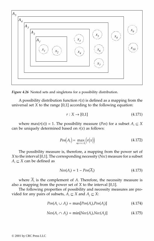
A possibility distribution function r(x) is defined as a mapping from theuniversal set X to the range [0,1] according to the following equation:
r : X → [0,1] (4.171)
where max(r(x)) = 1. The possibility measure (Pos) for a subset Ai ⊆ Xcan be uniquely determined based on r(x) as follows:
(4.172)
The possibility measure is, therefore, a mapping from the power set ofX to the interval [0,1]. The corresponding necessity (Nec) measure for a subsetAi ⊆ X can be defined as
Nes(Ai) = 1 – Pos(Ai) (4.173)
where Ai is the complement of A. Therefore, the necessity measure isalso a mapping from the power set of X to the interval [0,1].
The following properties of possibility and necessity measures are pro-vided for any pairs of subsets, Ai ⊆ X and Aj ⊆ X:
Pos(Ai ∪ Aj) = max[Pos(Ai),Pos(Aj)] (4.174)
Nes(Ai ∩ Aj) = min[Nec(Ai),Nec(Aj)] (4.175)
Figure 4.26 Nested sets and singletons for a possibility distribution.
A1x3
x2
A2
x1 x4
A3
x5
x6
x7
A4
x8
A5
x9
x10
Pos A r xix Ai
( ) = ( )( )∈
maxa µ
© 2001 by CRC Press LLC
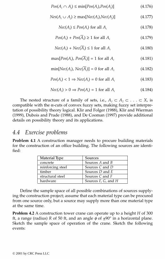
Pos(Ai ∩ Aj) ≤ min[Pos(Ai),Pos(Aj)] (4.176)
Nes(Ai ∪ Aj) ≥ max[Nec(Ai),Nec(Aj)] (4.177)
Nec(Ai) ≤ Pos(Ai) for all Ai (4.178)
Pos(Ai) + Pos(Ai) ≥ 1 for all Ai (4.179)
Nec(Ai) + Nec(Ai) ≤ 1 for all Ai (4.180)
max[Pos(Ai), Pos(Ai)] = 1 for all Ai (4.181)
min[Nec(Ai), Nec(Ai)] = 0 for all Ai (4.182)
Pos(Ai) < 1 ⇒ Nec(Ai) = 0 for all Ai (4.183)
Nec(Ai) > 0 ⇒ Pos(Ai) = 1 for all Ai (4.184)
The nested structure of a family of sets, i.e., A1 ⊂ A2 ⊂ . . . ⊂ X, iscompatible with the α-cuts of convex fuzzy sets, making fuzzy set interpre-tation of possibility theory logical. Klir and Folger (1988), Klir and Wierman(1999), Dubois and Prade (1988), and De Cooman (1997) provide additionaldetails on possibility theory and its applications.
4.4 Exercise problemsProblem 4.1 A construction manager needs to procure building materialsfor the construction of an office building. The following sources are identi-fied:
Define the sample space of all possible combinations of sources supply-ing the construction project; assume that each material type can be procuredfrom one source only, but a source may supply more than one material typeat the same time.
Problem 4.2 A construction tower crane can operate up to a height H of 300ft, a range (radius) R of 50 ft, and an angle φ of +90° in a horizontal plane.Sketch the sample space of operation of the crane. Sketch the followingevents:
Material Type Sourcesconcrete Sources A and Breinforcing steel Sources C and Dtimber Sources D and Estructural steel Sources C and Fhardware Sources F, G, and H
© 2001 by CRC Press LLC
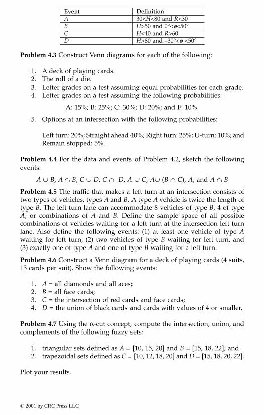
Problem 4.3 Construct Venn diagrams for each of the following:
1. A deck of playing cards.2. The roll of a die.3. Letter grades on a test assuming equal probabilities for each grade.4. Letter grades on a test assuming the following probabilities:
A: 15%; B: 25%; C: 30%; D: 20%; and F: 10%.
5. Options at an intersection with the following probabilities:
Left turn: 20%; Straight ahead 40%; Right turn: 25%; U-turn: 10%; andRemain stopped: 5%.
Problem 4.4 For the data and events of Problem 4.2, sketch the followingevents:
A ∪ B, A ∩ B, C ∪ D, C ∩ D, A ∪ C, A∪ (B ∩ C), A, and A ∩ B
Problem 4.5 The traffic that makes a left turn at an intersection consists oftwo types of vehicles, types A and B. A type A vehicle is twice the length oftype B. The left-turn lane can accommodate 8 vehicles of type B, 4 of typeA, or combinations of A and B. Define the sample space of all possiblecombinations of vehicles waiting for a left turn at the intersection left turnlane. Also define the following events: (1) at least one vehicle of type Awaiting for left turn, (2) two vehicles of type B waiting for left turn, and(3) exactly one of type A and one of type B waiting for a left turn.
Problem 4.6 Construct a Venn diagram for a deck of playing cards (4 suits,13 cards per suit). Show the following events:
1. A = all diamonds and all aces;2. B = all face cards;3. C = the intersection of red cards and face cards;4. D = the union of black cards and cards with values of 4 or smaller.
Problem 4.7 Using the α-cut concept, compute the intersection, union, andcomplements of the following fuzzy sets:
1. triangular sets defined as A = [10, 15, 20] and B = [15, 18, 22]; and2. trapezoidal sets defined as C = [10, 12, 18, 20] and D = [15, 18, 20, 22].
Plot your results.
Event DefinitionA 30<H<80 and R<30B H>50 and 0°<φ<50°C H<40 and R>60D H>80 and –30°<φ <50°
© 2001 by CRC Press LLC
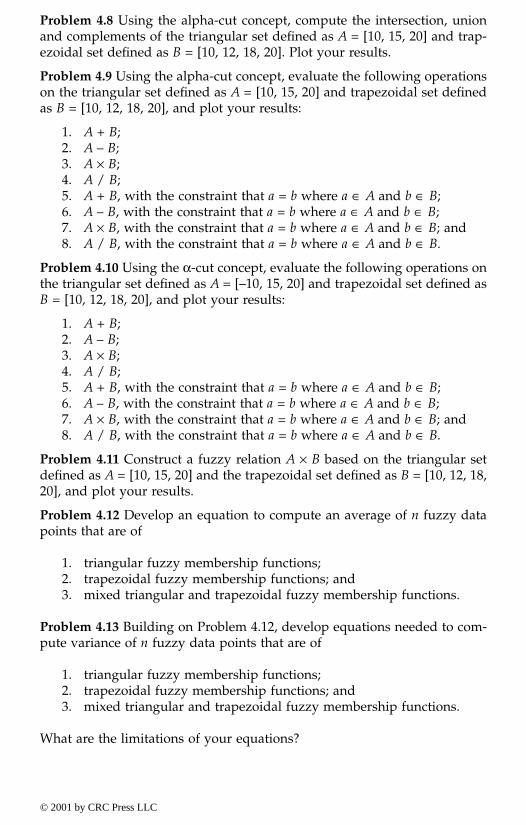
Problem 4.8 Using the alpha-cut concept, compute the intersection, unionand complements of the triangular set defined as A = [10, 15, 20] and trap-ezoidal set defined as B = [10, 12, 18, 20]. Plot your results.
Problem 4.9 Using the alpha-cut concept, evaluate the following operationson the triangular set defined as A = [10, 15, 20] and trapezoidal set definedas B = [10, 12, 18, 20], and plot your results:
1. A + B;2. A – B;3. A × B;4. A / B;5. A + B, with the constraint that a = b where a ∈ A and b ∈ B;6. A – B, with the constraint that a = b where a ∈ A and b ∈ B;7. A × B, with the constraint that a = b where a ∈ A and b ∈ B; and8. A / B, with the constraint that a = b where a ∈ A and b ∈ B.
Problem 4.10 Using the α-cut concept, evaluate the following operations onthe triangular set defined as A = [–10, 15, 20] and trapezoidal set defined asB = [10, 12, 18, 20], and plot your results:
1. A + B;2. A – B;3. A × B;4. A / B;5. A + B, with the constraint that a = b where a ∈ A and b ∈ B;6. A – B, with the constraint that a = b where a ∈ A and b ∈ B;7. A × B, with the constraint that a = b where a ∈ A and b ∈ B; and8. A / B, with the constraint that a = b where a ∈ A and b ∈ B.
Problem 4.11 Construct a fuzzy relation A × B based on the triangular setdefined as A = [10, 15, 20] and the trapezoidal set defined as B = [10, 12, 18,20], and plot your results.
Problem 4.12 Develop an equation to compute an average of n fuzzy datapoints that are of
1. triangular fuzzy membership functions;2. trapezoidal fuzzy membership functions; and 3. mixed triangular and trapezoidal fuzzy membership functions.
Problem 4.13 Building on Problem 4.12, develop equations needed to com-pute variance of n fuzzy data points that are of
1. triangular fuzzy membership functions;2. trapezoidal fuzzy membership functions; and 3. mixed triangular and trapezoidal fuzzy membership functions.
What are the limitations of your equations?
© 2001 by CRC Press LLC

Problem 4.14 Provide an example unknown set, and function that can berepresented by a rough set and a rough function, respectively.
Problem 4.15 Assume that the x’s represent users or intruders of an infor-mation network with specific nested characteristics such as x1 = a legitimateuser from an authorized IP address, x2 = an intruder from an authorized IPaddress or an intruder from an IP address that is masked by an authorizedIP address, x3 = a legitimate user with an authorized access protocol (user-name and password), and x4 = an intruder from an authorized IP accessprotocol. The nested structure of Figure 4.26 can be used to construct evi-dence gathering methods and their probabilities of affirmative detection,false detection, affirmative nondetection, and false nondetection. These prob-abilities can be constructed as basic assignments to meet the requirementsof the theory of evidence. They are then used to compute belief and plausi-bility measures for having any of the events A1 . . . A5 of Figure 4.26. Developthe mathematical formulation needed for this application with an illustrativeexample.
Problem 4.16 Two judges classified a case to three possible motivations asprovided in the following table in the form of basic assignments m1 and m2:
Compute the belief measures for judges 1 and 2. Compute the basic assign-ment for the combined judgment and the corresponding belief measure.
Problem 4.17 Two experts classified three possible causes for a bird speciespopulation decline, as provided in the following table, in the form of basicassignments m1 and m2:
Subset Judge 1 Judge 2(i.e., Motivation) m1 m2
Greed (G) 0.05 0.15Love (L) 0.10 0.05Self defense (S) 0.15 0.05G ∪ L 0.25 0.15G ∪ S 0.15 0.20L ∪ S 0.05 0.30G ∪ L ∪ S Not provided Not provided
Subset Expert 1 Expert 2(i.e., Cause) m1 m2
Changes in land use (C) 0.10 0.15Hunting (H) 0.15 0.15Disease (D) 0.15 0.15C ∪ H 0.25 0.15C ∪ D 0.15 0.10H ∪ D 0.15 0.20C ∪ H ∪ D Not provided Not provided
© 2001 by CRC Press LLC
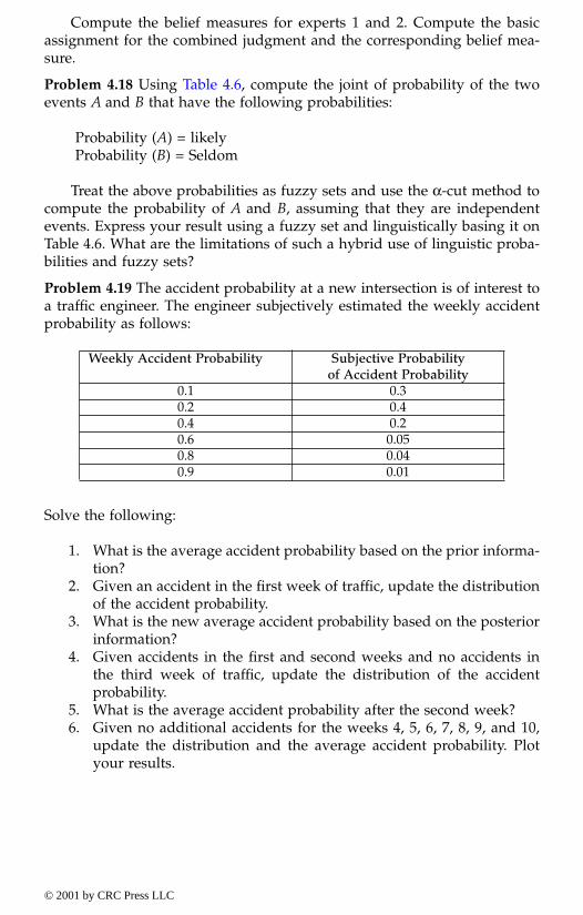
Compute the belief measures for experts 1 and 2. Compute the basicassignment for the combined judgment and the corresponding belief mea-sure.
Problem 4.18 Using Table 4.6, compute the joint of probability of the twoevents A and B that have the following probabilities:
Probability (A) = likelyProbability (B) = Seldom
Treat the above probabilities as fuzzy sets and use the α-cut method tocompute the probability of A and B, assuming that they are independentevents. Express your result using a fuzzy set and linguistically basing it onTable 4.6. What are the limitations of such a hybrid use of linguistic proba-bilities and fuzzy sets?
Problem 4.19 The accident probability at a new intersection is of interest toa traffic engineer. The engineer subjectively estimated the weekly accidentprobability as follows:
Solve the following:
1. What is the average accident probability based on the prior informa-tion?
2. Given an accident in the first week of traffic, update the distributionof the accident probability.
3. What is the new average accident probability based on the posteriorinformation?
4. Given accidents in the first and second weeks and no accidents inthe third week of traffic, update the distribution of the accidentprobability.
5. What is the average accident probability after the second week?6. Given no additional accidents for the weeks 4, 5, 6, 7, 8, 9, and 10,
update the distribution and the average accident probability. Plotyour results.
Weekly Accident Probability Subjective Probabilityof Accident Probability
0.1 0.30.2 0.40.4 0.20.6 0.050.8 0.040.9 0.01
© 2001 by CRC Press LLC
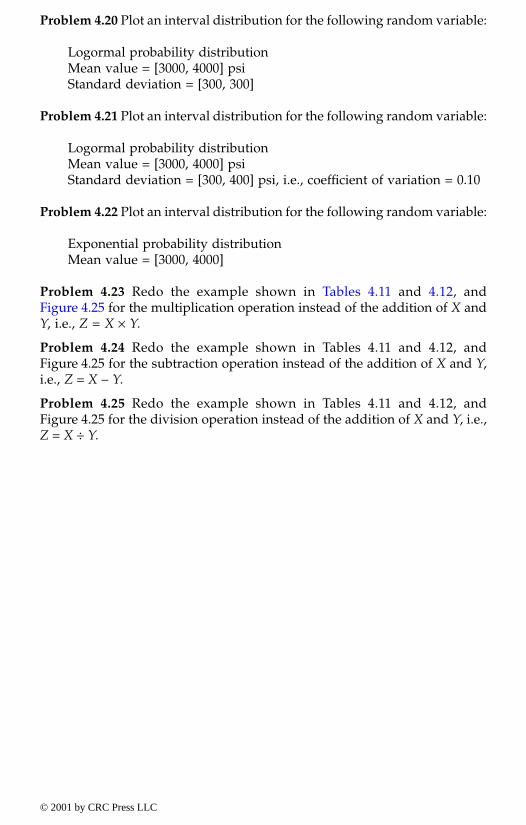
Problem 4.20 Plot an interval distribution for the following random variable:
Logormal probability distributionMean value = [3000, 4000] psiStandard deviation = [300, 300]
Problem 4.21 Plot an interval distribution for the following random variable:
Logormal probability distributionMean value = [3000, 4000] psiStandard deviation = [300, 400] psi, i.e., coefficient of variation = 0.10
Problem 4.22 Plot an interval distribution for the following random variable:
Exponential probability distributionMean value = [3000, 4000]
Problem 4.23 Redo the example shown in Tables 4.11 and 4.12, andFigure 4.25 for the multiplication operation instead of the addition of X andY, i.e., Z = X × Y.
Problem 4.24 Redo the example shown in Tables 4.11 and 4.12, andFigure 4.25 for the subtraction operation instead of the addition of X and Y,i.e., Z = X – Y.
Problem 4.25 Redo the example shown in Tables 4.11 and 4.12, andFigure 4.25 for the division operation instead of the addition of X and Y, i.e.,Z = X ÷ Y.
© 2001 by CRC Press LLC

chapter five
Consensus and aggregating expert opinions
Contents
5.1. Introduction5.2. Methods of scoring of expert opinions
5.2.1. Self scoring5.2.2. Collective scoring
5.3. Uncertainty measures5.3.1. Types of uncertainty measures5.3.2. Nonspecificity measures5.3.3. Entropy-like measures
5.3.3.1. Shannon entropy for probability theory5.3.3.2. Discrepancy measure5.3.3.3. Entropy measures for evidence theory
5.3.4. Fuzziness measure5.3.5. Other measures
5.4. Combining expert opinions5.4.1. Consensus combination of opinions5.4.2. Percentiles for combining opinions5.4.3. Weighted combinations of opinions5.4.4. Uncertainty-based criteria for combining expert opinions
5.4.4.1. Minimum uncertainty criterion5.4.4.2. Maximum uncertainty criterion5.4.4.3. Uncertainty invariance criterion
5.4.5. Opinion aggregation using interval analysisand fuzzy arithmetic
5.4.6. Opinion aggregation using Dempster’s ruleof combination
5.4.7. Demonstrative examples of aggregating expert opinions5.4.7.1. Aggregation of expert opinions5.4.7.2. Failure classification
5.5. Exercise problems
© 2001 by CRC Press LLC
5.1 IntroductionChapter 1 provides background materials on the definitions of knowledge,ignorance, information, uncertainty, and expert opinions. Experts rendersubjective opinions based on existing knowledge and information availableto them. Consequently, expert opinions can be viewed as preliminary prop-ositions with claims that are not fully justified or are justified with adequatereliability but are not infallible. In other words, expert opinions are seeds ofpropositional knowledge that do not meet one or more of the conditionsrequired for the justified true belief (JTB) within the framework of the reli-ability theory of knowledge. Despite the uncertainties associated with expertopinions, we consider them valuable since they might lead to knowledgeexpansion or evolution. In engineering and science, decisions commonlyneed to be made based on these opinions. These decisions can be consideredrisky, especially in cases of expert opinions with a lot of uncertainty, includ-ing conflicting or confusing opinions. Such decision situations structuredusing preliminary propositions can lead to adverse outcomes as some of thepropositions might be proved false. The relationships among knowledge,information, opinions, and evolutionary epistemology are schematicallyshown in Figure 1.6. The dialectic processes include communication methodssuch as languages, visual and audio formats, and other forms. It is commonin situations of high uncertainty to utilize multiple experts and assess thereliability of the experts (i.e., the sources of the opinions) using scoringmethods. Also, once the expert opinions are gathered, the uncertainty con-tents in these opinions individually and collectively need to be measured,and a final opinion needs to be produced through consensus or aggregation.
The objective of this chapter is to present methods for assessing orscoring expert opinions, measuring the uncertainty contents in individualopinions, aggregated or combined opinions, and selecting an optimal opin-ion. The methods presented are based on developments in expert opinionelicitation and uncertainty-based information of information science.
5.2 Methods of scoring of expert opinionsScoring methods can be used to assess the information reliability (or quality)provided by experts through an expert-opinion elicitation process. Theresulting scores can then be used for various applications, for example, todetermine weight factors for combining expert opinions if needed. Scoringmethods depend on the experts to assess either the reliability of their opin-ions or those of other experts; however, such approaches are like having afox guarding a henhouse.
5.2.1 Self scoring
According to this method, each expert provides a self-assessment in the formof a confidence level for each probability or answer provided for an issue.
© 2001 by CRC Press LLC

The primary disadvantages of this method are bias and overconfidence thatcan result in inaccurate self assessments. The method has the advantage ofsimplicity that can be viewed as commensurate to the nature of use of expert-opinion elicitation.
5.2.2 Collective scoring
According to this method, each expert provides assessments of other experts’opinions in the form of confidence levels in their provided probabilities oranswers related to an issue. The primary disadvantages of this method arebias and nonreproducibility. The bias in this case can be in an oppositedirection to the bias that might result from the self-scoring method — forexample, an underestimation versus an overestimation.
5.3 Uncertainty measures5.3.1 Types of uncertainty measures
We have presented several uncertainty types in Chapter 4 that were modeledusing various theories, such as probability, possibility, and evidence. Engi-neers and scientists would find great benefit in having measures to quantifythese uncertainties. These measures would be similar to measuring physicalquantities, such as temperature, pressure, or dimensions; however, they areunique in that they measure conceived or abstract notions rather than aphysical quantity. These uncertainty measures can be defined to be nonne-gative real numbers and should be inversely proportional to the strengthand consistency in evidence as expressed in the theory employed, i.e., thestronger and more consistent the evidence, the smaller the amount of uncer-tainty (Klir and Wierman, 1999). Such uncertainty measures should be suit-able to assess opinions rendered by one expert on some issue of interest, oropinions rendered by several experts on the same issue.
The area of uncertainty measures is not fully developed, and so is anactive research area (Klir and Wierman, 1999). Uncertainty measures weresuggested for some uncertainty types and theories covered in this chapter.This section limits itself to three relatively mature uncertainty types:(1) nonspecificity that results from imprecision connected with set sizes —cardinalities — and can be represented by the Hartley-like measure;(2) likelihood that results from various basic assignments represented byEntropy-like uncertainty measures; and (3) fuzziness as a result of vagueness.Engineering and science problems and expert opinions can simultaneouslycontain these uncertainty types and others.
5.3.2 Nonspecificity measures
A fundamental uncertainty type stems from lack of specificity as a result ofproviding several alternatives, with one alternative being the true one. This
© 2001 by CRC Press LLC

uncertainty type vanishes, and complete certainty is achieved, when onealternative is presented. Therefore, the nonspecificity uncertainty type resultsfrom having imprecision due to alternative sets that have cardinalitiesgreater than one. This fundamental measure can therefore be defined for afinite set of all possible alternatives, i.e., universal space X of alternativesunder consideration, with only one of the alternatives being correct, althoughthe correct alternative is unknown to us. However, we know based on allavailable evidence that the true alternative is in a subset A of X. In this case,only the alternatives that belong to A are considered as possible candidatesfor this true alternative. A measure of the amount of uncertainty associatedwith any finite set A of possible alternatives can be defined using the Hartleymeasure (H) as follows (Hartley, 1928):
H(A) = log2(|A|) (5.1)
where |A| is the cardinality of A, and log2 is the logarithm to the base2 resulting in a measurement unit in bits. A bit is a single digit in a binarynumber system and can be viewed as a unit of information equal to theamount of information obtained by learning or by resolving which of twoequally likely events has occurred. In computer language, bits form the basisof a byte, a string of binary digits (bits), usually eight, operated on as a basicunit by a digital computer. The logarithm (log2) of i as given by
log2(i) = x (5.2a)
is the power to which the base, in this case 2, must be raised to obtaini as provided by
2x = i (5.2b)
Chapter 4 provided cases that involve classifying an element to a familyof subsets using the theory of evidence. The nonspecificity in evidence canbe constructed be extending the Hartley measure to each subset, and com-puting a weighted sum of all the resulting measures of the subsets using thebasic assignment as weight factors. The nonspecificity measure can thereforebe defined for a basic assignment m for a family of subsets, A1, A2, . . ., An
∈ PX, according to the theory of evidence (He) as follows:
(5.3)
Equation 5.3 provides an assessment of the nonspecificity in evidence.The nonspecificity in an evidence results from associating the basic assign-
H m m A Ae i ii
n
( ) = ( ) ( )=∑ log2
1
© 2001 by CRC Press LLC
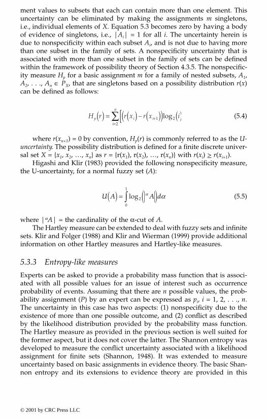
ment values to subsets that each can contain more than one element. Thisuncertainty can be eliminated by making the assignments m singletons,i.e., individual elements of X. Equation 5.3 becomes zero by having a bodyof evidence of singletons, i.e., |Ai| = 1 for all i. The uncertainty herein isdue to nonspecificity within each subset Ai, and is not due to having morethan one subset in the family of sets. A nonspecificity uncertainty that isassociated with more than one subset in the family of sets can be definedwithin the framework of possibility theory of Section 4.3.5. The nonspecific-ity measure Hp for a basic assignment m for a family of nested subsets, A1,A2, . . ., An ∈ PX, that are singletons based on a possibility distribution r(x)can be defined as follows:
(5.4)
where r(xn+1) = 0 by convention, Hp(r) is commonly referred to as the U-uncertainty. The possibility distribution is defined for a finite discrete univer-sal set X = {x1, x2, …, xn} as r = {r(x1), r(x2), …, r(xn)} with r(xi) > r(xi+1).
Higashi and Klir (1983) provided the following nonspecificity measure,the U-uncertainty, for a normal fuzzy set (A):
(5.5)
where |αA| = the cardinality of the α-cut of A.The Hartley measure can be extended to deal with fuzzy sets and infinite
sets. Klir and Folger (1988) and Klir and Wierman (1999) provide additionalinformation on other Hartley measures and Hartley-like measures.
5.3.3 Entropy-like measures
Experts can be asked to provide a probability mass function that is associ-ated with all possible values for an issue of interest such as occurrenceprobability of events. Assuming that there are n possible values, the prob-ability assignment (P) by an expert can be expressed as pi, i = 1, 2, . . ., n.The uncertainty in this case has two aspects: (1) nonspecificity due to theexistence of more than one possible outcome, and (2) conflict as describedby the likelihood distribution provided by the probability mass function.The Hartley measure as provided in the previous section is well suited forthe former aspect, but it does not cover the latter. The Shannon entropy wasdeveloped to measure the conflict uncertainty associated with a likelihoodassignment for finite sets (Shannon, 1948). It was extended to measureuncertainty based on basic assignments in evidence theory. The basic Shan-non entropy and its extensions to evidence theory are provided in this
H r r x r x ip i ii
n
( ) = ( ) ( )( ) ( )[ +=∑ – 1 2
2
log
U A A d( ) = ( )∫ log20
1α α
© 2001 by CRC Press LLC
section. Many attempts were made to generalize the Shannon entropy inevidence theory and other theories, but they have had limited success.Suggested models in this area are called entropy-like measures and are notfully mature for the purposes of this book.
5.3.3.1 Shannon entropy for probability theoryShannon (1948) provided an uncertainty measure for conflict that arises froma probability mass function that is commonly known as the entropy measureor the Shannon entropy measure. The entropy measure S(P) measure is givenby
(5.6)
This entropy measure takes on values from 0 to 1. Its value is zero if pi
= 1 and n = 1, and it is one for equally likely outcomes of pi = 1/n for all i.Klir and Folger (1988), and Klir and Wierman (1999) provide more detailson this measure. For a continuous random variable, the entropy is called theBoltzman (1894) entropy as given by (Harr, 1987):
(5.7)
where a = lower limit, b = upper limit, and f = probability densityfunction.
5.3.3.2 Discrepancy measureAn expert can be used to estimate a probability mass function (P) expressedas pi, i = 1, 2, . . ., n. This function is an estimate of a true, yet unknown,probability mass function (S) expressed as si, i = 1, 2, . . ., n. The discrepancymeasure is between the true and provided probability values as given by
(5.8)
This discrepancy measure (SD) is based on the Shannon entropy measure.The discrepancy measure can be used to obtain assessments of opinionsobtained from a set of experts with equal circumstances and conditions,although equal circumstances and conditions might not be attainable. Thediscrepancy measure provides an assessment of the degree of surprise thatsomeone would experience if an estimate pi, i = 1, 2, . . ., n is obtained whereasthe real values are si, i = 1, 2, . . ., n (Cooke, 1991).
S P p pi ii
n
( ) = ( )=∑– log2
1
B f f x f x dxX
a
b
X( ) = ( ) ( )( )∫– log2
S S P sspD i
i
ni
i
, –( ) =
=
∑ log22
© 2001 by CRC Press LLC
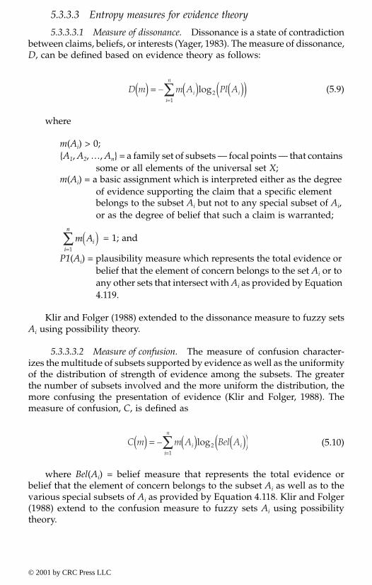
5.3.3.3 Entropy measures for evidence theory
5.3.3.3.1 Measure of dissonance. Dissonance is a state of contradictionbetween claims, beliefs, or interests (Yager, 1983). The measure of dissonance,D, can be defined based on evidence theory as follows:
(5.9)
where
m(Ai) > 0;{A1, A2, …, An} = a family set of subsets — focal points — that contains
some or all elements of the universal set X;m(Ai) = a basic assignment which is interpreted either as the degree
of evidence supporting the claim that a specific element belongs to the subset Ai but not to any special subset of Ai,or as the degree of belief that such a claim is warranted;
= 1; and
P1(Ai) = plausibility measure which represents the total evidence or belief that the element of concern belongs to the set Ai or to any other sets that intersect with Ai as provided by Equation 4.119.
Klir and Folger (1988) extended to the dissonance measure to fuzzy setsAi using possibility theory.
5.3.3.3.2 Measure of confusion. The measure of confusion character-izes the multitude of subsets supported by evidence as well as the uniformityof the distribution of strength of evidence among the subsets. The greaterthe number of subsets involved and the more uniform the distribution, themore confusing the presentation of evidence (Klir and Folger, 1988). Themeasure of confusion, C, is defined as
(5.10)
where Bel(Ai) = belief measure that represents the total evidence orbelief that the element of concern belongs to the subset Ai as well as to thevarious special subsets of Ai as provided by Equation 4.118. Klir and Folger(1988) extend to the confusion measure to fuzzy sets Ai using possibilitytheory.
D m m A Pl Ai ii
n
( ) = ( ) ( )( )=∑– log2
1
m Aii
n
( )=∑
1
C m m A Bel Ai ii
n
( ) = ( ) ( )( )=∑– log2
1
© 2001 by CRC Press LLC

5.3.4 Fuzziness measure
Fuzziness as represented by fuzzy set theory results from uncertainty inbelonging to a set or notion. Fuzzy sets are sets that have fuzzy boundaries.For a given fuzzy set A, each element x of the universal set X has a mem-bership value µA(x) to A that represents the degree of belief that x belongsto A or can be viewed as a measure of compatibility between x and the notionof A. The membership value is in the range [0,1] as described in Section 4.2.3.The vagueness uncertainty type can be assessed based on the fuzzy bound-aries of the set A. A set A is considered fuzzier than set B if the boundaryof A becomes wider than the boundaries of B in defining the transition frombelonging to nonbelonging to the set. In addition, a fuzzy set has a uniqueproperty of having a nonempty intersection with its complement. Yager (1979and 1980b) use these interpretations of fuzziness in suggesting a measurefor it as follows:
(5.11)
f = fuzziness measure of a fuzzy set A; X = universal set; A = complementof A; µA(x) is membership value of x to A. Using the definition of the com-plement provided by Equation 4.52, Equation 5.11 can be written as
(5.12)
The fuzziness measure becomes zero as the set becomes crisp with µA(x)taking only values of zeros and ones and reaches maximum at µA(x) = 0.5.
5.3.5 Other measures
Klir and Wierman (1999) describe other uncertainty measures, such as thediscord measure and strife measure based on evidence theory and possibilitytheory. They also provide methods to aggregate uncertainty based on evi-dence theory, fuzzy entropy based on fuzzy set theory, and generalizedmeasure based on fuzzified evidence theory.
5.4 Combining expert opinionsIn some applications, expert opinions in the form of subjective probabilitiesof an event need to be combined into a single value and perhaps intervalsfor their use in probabilistic and risk analyses. Cooke (1991) and Rowe (1992)provide a summary of methods for combining expert opinions. The methodscan be classified into consensus methods and mathematical methods(Clemen, 1989; Ferrell, 1985). The mathematical methods can be based on
f A X x xA Ax X
( ) = ( ) ( )∈∑– –µ µ
f A X xAx X
( ) = ( )∈∑– –2 1µ
© 2001 by CRC Press LLC

assigning equal weights or different weights to the experts. This sectionprovides a summary of methods for combining expert opinions.
5.4.1 Consensus combination of opinions
A consensus combination of opinion is obtained through a facilitated dis-cussion among the experts to some agreeable common values with perhapsa confidence interval or outer quartile values. The primary shortcomings ofthis method are (1) socially reinforced irrelevance or conformity within agroup, (2) dominance of strong-minded or strident individuals, (3) groupmotive of quickly reaching an agreement, and (4) group-reinforced bias dueto common background of group members. The facilitator of an expert-opinion elicitation session should play a major role in reducing group pres-sure, individual dominance, and biases.
5.4.2 Percentiles for combining opinions
A p-percentile value (xp) for a random variable based on a sample can bedefined as the value of the parameter such that p% of the data is less thanor equal to xp. On the basis of this definition, the median value is consideredto be the 50-percentile value. Aggregating the opinions of experts can bebased on computing the 25, 50, and 75 percentile values of the gatheredopinions. The computation of these values depends on the number of expertsproviding opinions. Table 4.7 provides a summary of the needed equationsfor 4 to 20 experts. For example, 7 experts provided the following subjectiveprobability of an event sorted in decreasing order:
Probabilities ={1.0E-02, 5.0E-03, 5.0E-03, 1.0E-03, 1.0E-03, 5.0E-04, 1.0E-04} (5.13)
The median and arithmetic quartile points according to Table 4.7 arerespectively given by
25 percentile = 5.0E-03 (5.14a)
50 percentile (median) = 1.0E-03 (5.14b)
75 percentile = 7.5E-04 (5.14c)
5.4.3 Weighted combinations of opinions
French (1985) and Genest and Zidek (1986) provide summaries of variousmethods for combining probabilities and example uses. For E experts withthe ith expert providing a vector of n probability values, p1i, p2i, . . ., pni, forsample space outcomes A1, A2, . . ., An, the E expert opinions can be combined
© 2001 by CRC Press LLC

using weight factors w1, w2, . . ., wE, that sum up to one, using one of thefollowing selected methods:
1. Weighted arithmetic average:The weighted arithmetic mean for outcome j can be computed as follows:
Weighted arithmetic mean for outcome (5.15)
The weighted arithmetic means are then normalized using their total toobtain the 1-norm probability for an outcome for each outcome as follows:
1-norm probability for outcome (5.16)
2. Weighted geometric average:The weighted geometric mean for outcome j can be computed as follows:
Weighted geometric mean for outcome (5.17)
The weighted geometric means are then normalized using their total toobtain the 0-norm probability for an outcome for each outcome as follows:
0-norm probability for outcome (5.18)
3. Weighted harmonic average:The weighted harmonic mean for outcome j can be computed as follows:
Weighted harmonic mean for outcome (5.19)
The weighted harmonic means are then normalized using their total toobtain the -1-norm probability for an outcome for each outcome as follows:
j M j w pi jii
E
= ( ) ==∑1
1
j P jM j
M kk
n= ( ) =
( )( )
=∑
11
11
j M j p ji
w
i
Ei= ( ) = ( )
=∏0
1
j P jM j
M kk
n= ( ) =
( )( )
=∑
00
01
j M jwp
i
jii
E= ( ) =
=∑
–1
1
1
© 2001 by CRC Press LLC
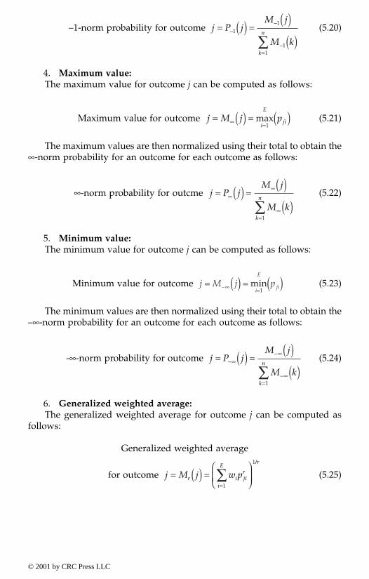
–1-norm probability for outcome (5.20)
4. Maximum value:The maximum value for outcome j can be computed as follows:
Maximum value for outcome (5.21)
The maximum values are then normalized using their total to obtain the∞-norm probability for an outcome for each outcome as follows:
∞-norm probability for outcme (5.22)
5. Minimum value:The minimum value for outcome j can be computed as follows:
Minimum value for outcome (5.23)
The minimum values are then normalized using their total to obtain the–∞-norm probability for an outcome for each outcome as follows:
-∞-norm probability for outcome (5.24)
6. Generalized weighted average:The generalized weighted average for outcome j can be computed as
follows:
Generalized weighted average
for outcome (5.25)
j P jM j
M kk
n= ( ) =
( )( )
=∑
––
–
11
11
j M j pi
E
ji= ( ) = ( )∞ =max
1
j P jM j
M kk
n= ( ) =
( )( )
∞∞
∞=
∑1
j M j pi
E
ji= ( ) = ( )∞ =– min1
j P jM j
M kk
n= ( ) =
( )( )
∞∞
∞=
∑–
–
–1
j M j w pr i jir
i
Er
= ( ) =
=∑
1
1/
© 2001 by CRC Press LLC

The generalized weighted for averages are then normalized usingtheir total to obtain the r-norm probability for an outcome each outcomeas follows:
r-norm probability for outcome (5.26)
where for r = 1, and –1, cases 1 and 3 result, respectively.
5.4.4 Uncertainty-based criteria for combining expert opinions
Expert opinions are propositions that do not necessarily meet the JTB require-ments of knowledge and, hence, can contain both useful information anduncertainties. In combining these opinions, we have a vested interest in usinga process that utilizes all the information contents provided by the expertsand that can account for the various uncertainties in producing a combinedopinion. The uncertainties can include nonspecificity, conflict, confusion,vagueness, biases, and varying reliability levels of sources, among othertypes.
Section 5.3 presents methods for measuring uncertainty. These measuresdeal with the various uncertainty types. In combining expert opinions, wecan develop expert-opinion aggregation methods that are either information-based or uncertainty-based. In fact, information and uncertainty can beargued to represent a duality, since information can be considered useful bya cognitive agent if this information results in reducing its uncertainty underprescribed conditions. Therefore, the amount of relevant information gainedby the agent is related and can be measured by the amount of uncertaintyreduced. This concept of uncertainty-based information was introduced byKlir (1985). The various uncertainty measures presented in this section candeal with various uncertainty types and offer strengths and weaknesses withcommensurate complexity and computational demands. The selection of anappropriate uncertainty measure or combinations thereof is problem depen-dent, and a tradeoff decision between the computational effort needed andthe return on this effort in the form of a refined combination of expertopinions needs to be made.
Three uncertainty-based criteria can be used to combine expert opinion:(1) minimum uncertainty, (2) maximum uncertainty, and (3) uncertaintyinvariance. These three criteria are described in subsequent sections. Thecriteria of minimum and maximum uncertainty were developed and hadgreat utilities in classical information theory and is commonly referred tothe principles of minimum and maximum entropy.
j P jM j
M kr
r
rk
n= ( ) =
( )( )
=∑
1
© 2001 by CRC Press LLC

5.4.4.1 Minimum uncertainty criterionEngineers and scientists have a need to select among alternative solutionsbased on information given on a problem where each solution has a differentlevel of information retention, bias, and error uncertainties. For example,curve fitting of an analytical model to empirical results commonly involvesthe computation of model parameters with each set of parameters leadingto various levels of information retention and uncertainty. An optimal solu-tion in this case can be defined as the solution that maximizes informationretention, i.e., minimizes uncertainty. The principle of least squares in regres-sion analysis is an example of such criterion. Other examples include sim-plification problems in order to deal with systems complexity, and conflictresolution problems in cases of gathering evidence in failure classification.
5.4.4.2 Maximum uncertainty criterionThe criterion of maximum uncertainty can be used in cases involving rea-soning that could lead to conclusions that are not necessarily entailed ingiven premises. In such cases, we should intuitively use all informationsupported by available evidence but without unintentionally adding infor-mation unsupported by the evidence given. This criterion employs the rela-tionship between information and uncertainty by requiring any conclusionresulting from any inference to maximize the relevant uncertainty withinconstraints representing given premises. As a result, we fully limit our infer-ence ability by our ignorance when making inferences beyond the premiseinformation domain, and we fully utilize information provided by the pre-mises. This criterion, therefore, provides use with assurances of maximizingour nonreliance on information not contained in the premises.
The criterion of maximum uncertainty appeals to engineers and scien-tists since it results in inferences and solutions that do not go beyond pre-mises given. For example, predictive, scientific models can be viewed asinference models using premises. In system identification, statements on asystem or subsystems need to be based on partial knowledge of the system;hence the need to make sure that our inferences do not go beyond informa-tion and premises available to us. In selecting a likelihood distribution, thecriterion of maximum uncertainty can provide the means of complete uncer-tainty retention and not assuming additional information beyond what isgiven to us.
Example 5.1 Selection of distribution types based on selected constraints using uncertainty measures
The criterion of maximum uncertainty can be used to select the distributiontype that maximizes uncertainty for given constraints. The entropy uncer-tainty measure was used for this purpose. Table 5.1 summarizes distributiontypes that maximize uncertainty for a selected list of constraints. For exam-ple, the constraints a < X < b and
© 2001 by CRC Press LLC

(5.27)
can be used to maximize the entropy according to Equation 5.7 as follows:
maximize (5.28)
Table 5.1 Maximum-Entropy Probability Distributions
ConstraintsMaximum-Entropy
Distribution
Minimum value = aMaximum value = b
Uniform
Expected value = X
Exponential
Expected value = XStandard deviation = S2
Normal
Expected value = XStandard deviation = S2
Finite range of a minimum value = a, and a maximum value = b
Beta
where pi = probability of i independent and identical events occurring in an interval T with an expected rate of occurrence of events of λ
Poisson
f x dxXa
b
( ) =∫ 1
f x dxX ( ) =∞
∫ 10
f x dxX ( ) =∞
∞
∫ 1–
f x dxXa
b
( ) =∫ 1
pii=
∞
∑ =1
1
f x dxXa
b
( ) =∫ 1
B f f x f x dxX Xa
b
( ) = ( ) ( )( )∫– ln
© 2001 by CRC Press LLC

Using the method of Lagrange multipliers, the following equation canbe obtained:
(5.29)
This equation has the following solutions:
–1 – ln(f) + λ = 0 (5.30a)
fX(x) = eλ –1 (5.30b)
Since λ is a constant, f must be a constant leading to the followingexpression for f:
(5.31)
The corresponding entropy is
B(f) = ln(b – a) (5.32)
5.4.4.3 Uncertainty invariance criterionThe criterion of uncertainty invariance was developed to facilitate meaning-ful transformations among various uncertainty measures. This criterion uti-lizes uncertainty measures that should be carefully constructed in terms ofscale and units to allow for transforming one uncertainty type to another;therefore, once all uncertainties are consistently measured, they can beadded, manipulated, and treated using a most convenient theory. The crite-rion of uncertainty invariance principle was used in probability-possibilitytransformations in combining objective and subjective information that arerepresented using probability and possibility theory (Brown, 1980).
5.4.5 Opinion aggregation using interval analysis and fuzzy arithmetic
Sometimes it might be desirable to elicit probabilities and/or consequencesusing linguistic terms as shown in Table 4.6 for linguistic probabilities. Lin-guistic terms of this type can be translated into intervals or fuzzy numbers.Intervals are considered a special case of fuzzy numbers which are in turna special case of fuzzy sets. Section 4.2.3 shows methods for performingfuzzy arithmetic and fuzzy calculus that can be used to combine expertopinions in this case.
–∂
∂ ( )( ) + ∂∂ ( ) =
ff f
ffln λ 0
f xb aX ( ) = 1
–
© 2001 by CRC Press LLC
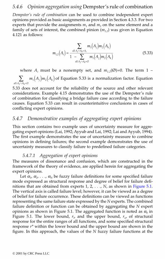
5.4.6 Opinion aggregation using Dempster’s rule of combination
Dempster’s rule of combination can be used to combine independent expertopinions provided as basic assignments as provided in Section 4.3.3. For twoexperts that provide the assignments m1 and m2 on the same element and afamily of sets of interest, the combined pinion (m1,2) was given in Equation4.121 as follows:
(5.33)
where Ai must be a nonempty set, and m1,2(Ø)=0. The term 1 –
of Equation 5.33 is a normalization factor. Equation
5.33 does not account for the reliability of the source and other relevantconsiderations. Example 4.15 demonstrates the use of the Dempster’s ruleof combination for classifying a bridge failure case according to the failurecauses. Equation 5.33 can result in counterintuitive conclusions in cases ofconflicting expert opinions.
5.4.7 Demonstrative examples of aggregating expert opinions
This section contains two example uses of uncertainty measure for aggre-gating expert opinions (Lai, 1992; Ayyub and Lai, 1992; Lai and Ayyub, 1994).The first example demonstrates the use of uncertainty measure to combineopinions in defining failures; the second example demonstrates the use ofuncertainty measures to classify failure to predefined failure categories.
5.4.7.1 Aggregation of expert opinionsThe measures of dissonance and confusion, which are constructed in theframework of the theory of evidence, are applied herein for aggregating theexpert opinions.
Let α1, α2, . . ., αN be fuzzy failure definitions for some specified failuremode expressed as structural response and degree of belief for failure defi-nitions that are obtained from experts 1, 2, . . ., N, as shown in Figure 5.1.The vertical axis is called failure level; however, it can be viewed as a degreeof belief for failure occurrence. These definitions can be viewed as functionsrepresenting the same failure state expressed by the N experts. The combinedfailure definition or function can be obtained by aggregating the N expertopinions as shown in Figure 5.1. The aggregated function is noted as α0 inFigure 5.1. The lower bound, rl, and the upper bound, ru, of structuralresponse for the entire ranges of all functions, and some specified structuralresponse r* within the lower bound and the upper bound are shown in thefigure. In this approach, the values of the N fuzzy failure functions at the
m A
m A m A
m A m Ai
j kA A A
j kA A
j k i
j k
1 2
1 2
1 21,
–( ) =
( ) ( )( ) ( )
∩ =
∩ =∅
∑∑
all
all
m A m Aj kA Aj k
1 2( ) ( )∩ =∅∑
all
© 2001 by CRC Press LLC
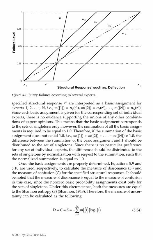
specified structural response r* are interpreted as a basic assignment forexperts 1, 2, . . ., N, i.e., m({1}) = α1(r*), m({2}) = α2(r*),. . ., m({N}) = αN(r*).Since each basic assignment is given for the corresponding set of individualexperts, there is no evidence supporting the unions of any other combina-tions of expert opinions. This means that the basic assignment correspondsto the sets of singletons only; however, the summation of all the basic assign-ments is required to be equal to 1.0. Therefore, if the summation of the basicassignment does not equal 1.0, i.e., m({1}) + m({2}) + . . . + m({N}) ≠ 1.0, thedifference between the summation of the basic assignment and 1 should bedistributed to the set of singletons. Since there is no particular preferencefor any set of individual experts, the difference should be distributed to thesets of singletons by normalization with respect to the summation, such thatthe normalized summation is equal to 1.0.
Once the basic assignments are properly determined, Equations 5.9 and5.10 are used, respectively, to calculate the measure of dissonance (D) andthe measure of confusion (C) for the specified structural responses. It shouldbe noted that the measure of dissonance is equal to the measure of confusionin this case, since the nonzero basic probability assignments exist only forthe sets of singletons. Under this circumstance, both the measures are equalto the Shannon entropy (S) (Shannon, 1948). Therefore, the measure of uncer-tainty can be calculated as the following:
(5.34)
Figure 5.1 Fuzzy failures according to several experts.
0
0.25
0.5
0.75
1
Structural Response, such as, Deflection
Failu
re L
evel
α 1 α 2 α 3
α 0
α N
r l r ur*
D C S m i ii
N
= = = { }( ) ( )=∑–
12log
© 2001 by CRC Press LLC
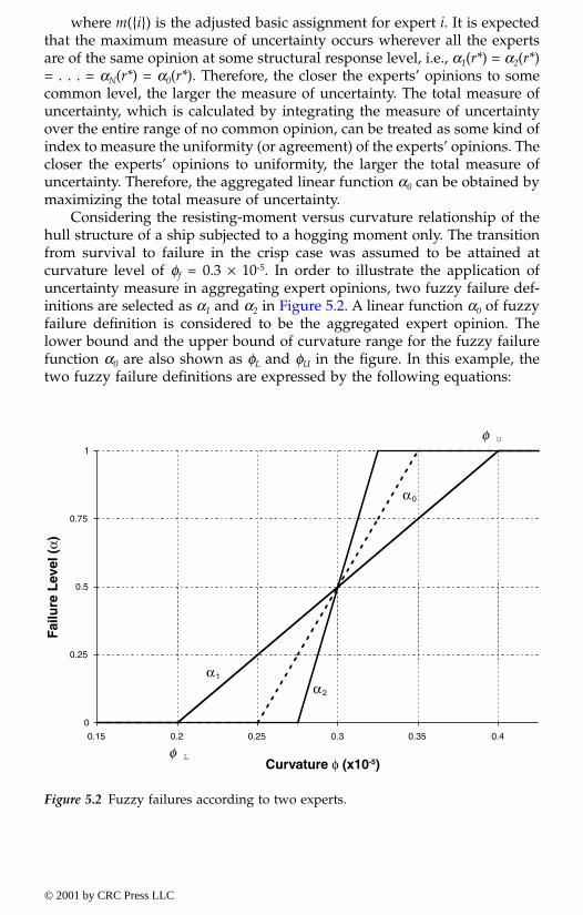
where m({i}) is the adjusted basic assignment for expert i. It is expectedthat the maximum measure of uncertainty occurs wherever all the expertsare of the same opinion at some structural response level, i.e., α1(r*) = α2(r*)= . . . = αN(r*) = α0(r*). Therefore, the closer the experts’ opinions to somecommon level, the larger the measure of uncertainty. The total measure ofuncertainty, which is calculated by integrating the measure of uncertaintyover the entire range of no common opinion, can be treated as some kind ofindex to measure the uniformity (or agreement) of the experts’ opinions. Thecloser the experts’ opinions to uniformity, the larger the total measure ofuncertainty. Therefore, the aggregated linear function α0 can be obtained bymaximizing the total measure of uncertainty.
Considering the resisting-moment versus curvature relationship of thehull structure of a ship subjected to a hogging moment only. The transitionfrom survival to failure in the crisp case was assumed to be attained atcurvature level of φf = 0.3 × 10⁻⁵. In order to illustrate the application ofuncertainty measure in aggregating expert opinions, two fuzzy failure def-initions are selected as α1 and α2 in Figure 5.2. A linear function α0 of fuzzyfailure definition is considered to be the aggregated expert opinion. Thelower bound and the upper bound of curvature range for the fuzzy failurefunction α0 are also shown as φL and φU in the figure. In this example, thetwo fuzzy failure definitions are expressed by the following equations:
Figure 5.2 Fuzzy failures according to two experts.
0
0.25
0.5
0.75
1
0.15 0.2 0.25 0.3 0.35 0.4
Curvature φ (x10-5)
Failu
re L
evel
(α)
α1
α2
α0
φ L
φ U
© 2001 by CRC Press LLC
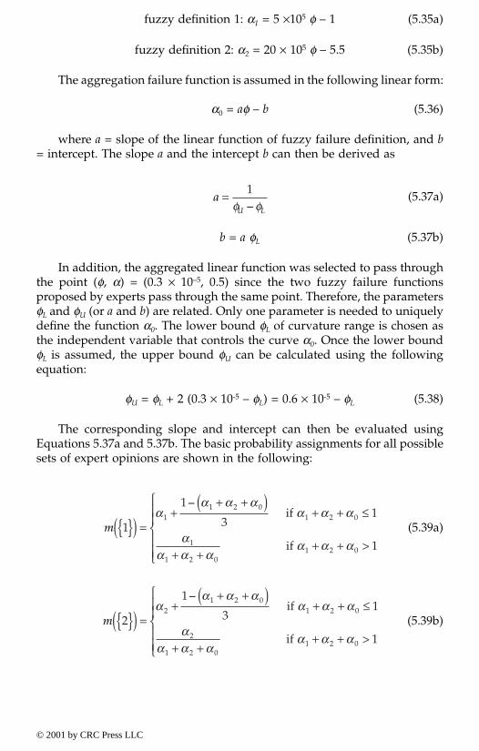
fuzzy definition 1: α1 = 5 ×10⁵ φ – 1 (5.35a)
fuzzy definition 2: α2 = 20 × 105 φ – 5.5 (5.35b)
The aggregation failure function is assumed in the following linear form:
α0 = aφ – b (5.36)
where a = slope of the linear function of fuzzy failure definition, and b= intercept. The slope a and the intercept b can then be derived as
(5.37a)
b = a φL (5.37b)
In addition, the aggregated linear function was selected to pass throughthe point (φ, α) = (0.3 × 10⁻⁵, 0.5) since the two fuzzy failure functionsproposed by experts pass through the same point. Therefore, the parametersφL and φU (or a and b) are related. Only one parameter is needed to uniquelydefine the function α0. The lower bound φL of curvature range is chosen asthe independent variable that controls the curve α0. Once the lower boundφL is assumed, the upper bound φU can be calculated using the followingequation:
φU = φL + 2 (0.3 × 10⁻⁵ – φL) = 0.6 × 10⁻⁵ – φL (5.38)
The corresponding slope and intercept can then be evaluated usingEquations 5.37a and 5.37b. The basic probability assignments for all possiblesets of expert opinions are shown in the following:
(5.39a)
(5.39b)
aU L
= 1φ φ–
m 1
1
31
1
11 2 0
1 2 0
1
1 2 01 2 0
{ }( ) =+
+ +( )+ + ≤
+ ++ + >
αα α α
α α α
αα α α
α α α
– if
if
m 2
1
31
1
21 2 0
1 2 0
2
1 2 01 2 0
{ }( ) =+
+ +( )+ + ≤
+ ++ + >
αα α α
α α α
αα α α
α α α
– if
if
© 2001 by CRC Press LLC
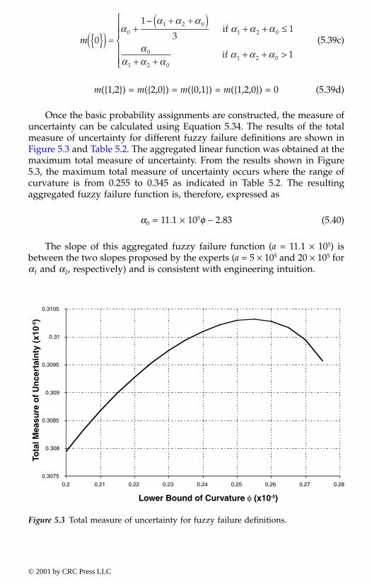
(5.39c)
m({1,2}) = m({2,0}) = m({0,1}) = m({1,2,0}) = 0 (5.39d)
Once the basic probability assignments are constructed, the measure ofuncertainty can be calculated using Equation 5.34. The results of the totalmeasure of uncertainty for different fuzzy failure definitions are shown inFigure 5.3 and Table 5.2. The aggregated linear function was obtained at themaximum total measure of uncertainty. From the results shown in Figure5.3, the maximum total measure of uncertainty occurs where the range ofcurvature is from 0.255 to 0.345 as indicated in Table 5.2. The resultingaggregated fuzzy failure function is, therefore, expressed as
α0 = 11.1 × 10⁵φ – 2.83 (5.40)
The slope of this aggregated fuzzy failure function (a = 11.1 × 10⁵) isbetween the two slopes proposed by the experts (a = 5 × 10⁵ and 20 × 105 forα1 and α2, respectively) and is consistent with engineering intuition.
Figure 5.3 Total measure of uncertainty for fuzzy failure definitions.
m 0
1
31
1
01 2 0
1 2 0
0
1 2 01 2 0
{ }( ) =+
+ +( )+ + ≤
+ ++ + >
αα α α
α α α
αα α α
α α α
– if
if
0.3075
0.308
0.3085
0.309
0.3095
0.31
0.3105
0.2 0.21 0.22 0.23 0.24 0.25 0.26 0.27 0.28
Lower Bound of Curvature φ (x10-5)
Tota
l Mea
sure
of
Un
cert
ain
ty (
x10-5
)
© 2001 by CRC Press LLC
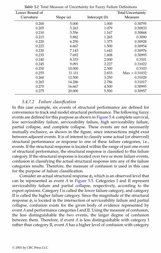
5.4.7.2 Failure classificationIn this case example, six events of structural performance are defined forconvenience to track and model structural performance. The following fuzzyevents are defined for this purpose as shown in Figure 5.4: complete survival,low serviceability failure, serviceability failure, high serviceability failure,partial collapse, and complete collapse. These events are not necessarilymutually exclusive, as shown in the figure, since intersections might existbetween adjacent events. It is of interest to classify some actual (or observed)structural performance or response to one of these failure categories, i.e.,events. If the structural response is located within the range of just one eventof structural performance, the structural response is classified to this failurecategory. If the structural response is located over two or more failure events,confusion in classifying the actual structural response into any of the failurecategories results. Therefore, the measure of confusion is used in this casefor the purpose of failure classification.
Consider an actual structural response φA which is an observed level thatcan be represented as event A in Figure 5.5. Categories I and II representserviceability failure and partial collapse, respectively, according to theexpert opinions. Category I is called the lower failure category, and categoryII is called the higher failure category. Since the magnitude of the structuralresponse φA is located in the intersection of serviceability failure and partialcollapse, confusion exists for the given body of evidence represented byevent A and performance categories I and II. Using the measure of confusion,the less distinguishable the two events, the larger degree of confusionbetween them. Therefore, if event A is less distinguishable with category Irather than category II, event A has a higher level of confusion with category
Table 5.2 Total Measure of Uncertainty for Fuzzy Failure Definitions
Lower Bound of Curvature Slope (a) Intercept (b)
Total Uncertainty Measure
0.200 5.000 1.000 0.307950.205 5.263 1.079 0.308330.210 5.556 1.167 0.308680.215 5.882 1.265 0.30900.220 6.250 1.375 0.309280.225 6.667 1.500 0.309540.230 7.143 1.643 0.309760.235 7.692 1.808 0.309950.240 8.333 2.000 0.31010.245 9.091 2.227 0.310220.250 10.000 2.500 0.31030.255 11.111 2.833 Max = 0.310320.260 12.500 3.250 0.310280.265 14.286 2.786 0.310170.270 16.667 4.500 0.309950.275 20.000 5.500 0.30957
© 2001 by CRC Press LLC

Figure 5.4 Six events of structural response.
Figure 5.5 Failure events.
0
0.25
0.5
0.75
1
0.18 0.2 0.21 0.23 0.24 0.26 0.27 0.29 0.3 0.32 0.33 0.35 0.36 0.38 0.39 0.41 0.42
Curvature φ (x10-5)
Deg
ree
of
Bel
ief
(α)
Complete SurvivalLow Serviceability
FailureServiceability
FailureHigh Serviceability
Failure Partial Collapse Complete Collapse
© 2001 by CRC Press LLC
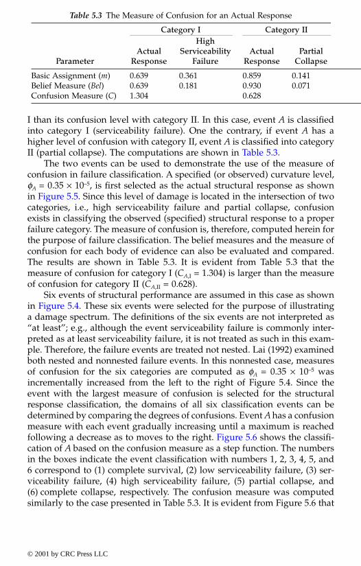
I than its confusion level with category II. In this case, event A is classifiedinto category I (serviceability failure). One the contrary, if event A has ahigher level of confusion with category II, event A is classified into categoryII (partial collapse). The computations are shown in Table 5.3.
The two events can be used to demonstrate the use of the measure ofconfusion in failure classification. A specified (or observed) curvature level,φA = 0.35 × 10⁻⁵, is first selected as the actual structural response as shownin Figure 5.5. Since this level of damage is located in the intersection of twocategories, i.e., high serviceability failure and partial collapse, confusionexists in classifying the observed (specified) structural response to a properfailure category. The measure of confusion is, therefore, computed herein forthe purpose of failure classification. The belief measures and the measure ofconfusion for each body of evidence can also be evaluated and compared.The results are shown in Table 5.3. It is evident from Table 5.3 that themeasure of confusion for category I (CA,I = 1.304) is larger than the measureof confusion for category II (CA,II = 0.628).
Six events of structural performance are assumed in this case as shownin Figure 5.4. These six events were selected for the purpose of illustratinga damage spectrum. The definitions of the six events are not interpreted as“at least”; e.g., although the event serviceability failure is commonly inter-preted as at least serviceability failure, it is not treated as such in this exam-ple. Therefore, the failure events are treated not nested. Lai (1992) examinedboth nested and nonnested failure events. In this nonnested case, measuresof confusion for the six categories are computed as φA = 0.35 × 10⁻⁵ wasincrementally increased from the left to the right of Figure 5.4. Since theevent with the largest measure of confusion is selected for the structuralresponse classification, the domains of all six classification events can bedetermined by comparing the degrees of confusions. Event A has a confusionmeasure with each event gradually increasing until a maximum is reachedfollowing a decrease as to moves to the right. Figure 5.6 shows the classifi-cation of A based on the confusion measure as a step function. The numbersin the boxes indicate the event classification with numbers 1, 2, 3, 4, 5, and6 correspond to (1) complete survival, (2) low serviceability failure, (3) ser-viceability failure, (4) high serviceability failure, (5) partial collapse, and(6) complete collapse, respectively. The confusion measure was computedsimilarly to the case presented in Table 5.3. It is evident from Figure 5.6 that
Table 5.3 The Measure of Confusion for an Actual Response
Category I Category II
ParameterActual
Response
HighServiceability
FailureActual
ResponsePartial
Collapse
Basic Assignment (m) 0.639 0.361 0.859 0.141Belief Measure (Bel) 0.639 0.181 0.930 0.071Confusion Measure (C) 1.304 0.628
© 2001 by CRC Press LLC

the classification of an event changes from a lower failure category to anadjacent higher failure category at a curvature level located near the inter-section of the two-adjacent failure categories.
5.5 Exercise problemsProblem 5.1 For the following probability mass function,
Compute (a) the Hartley uncertainty measure, and (b) the Shannonentropy uncertainty measure. Discuss their meanings.
Problem 5.2 For the following probability mass function:
Compute (a) the Hartley uncertainty measure, and (b) the Shannonentropy uncertainty measure. Discuss their meanings.
Figure 5.6 Classifying an actual response to the six events of structural response.
x 10 20 30 40 50PX(x) 0.40 0.30 0.20 0.05 0.05
x 1 2 3 4 5PX(x) 0.10 0.20 0.40 0.20 0.10
0
0.25
0.5
0.75
1
0.18 0.2 0.21 0.23 0.24 0.26 0.27 0.29 0.3 0.32 0.33 0.35 0.36 0.38 0.39 0.41 0.42
Curvature φ (x10-5)
Deg
ree
of
Bel
ief
(α)
Complete SurvivalLow Serviceability
FailureServiceability
FailureHigh Serviceability
Failure Partial Collapse Complete Collapse
1
2
3
4
5
6
© 2001 by CRC Press LLC
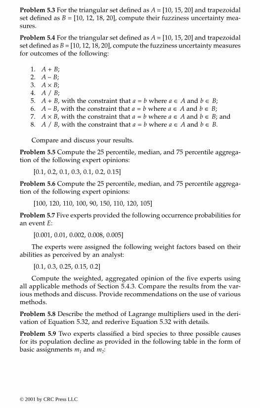
Problem 5.3 For the triangular set defined as A = [10, 15, 20] and trapezoidalset defined as B = [10, 12, 18, 20], compute their fuzziness uncertainty mea-sures.
Problem 5.4 For the triangular set defined as A = [10, 15, 20] and trapezoidalset defined as B = [10, 12, 18, 20], compute the fuzziness uncertainty measuresfor outcomes of the following:
1. A + B;2. A – B;3. A × B;4. A / B;5. A + B, with the constraint that a = b where a ∈ A and b ∈ B;6. A – B, with the constraint that a = b where a ∈ A and b ∈ B;7. A × B, with the constraint that a = b where a ∈ A and b ∈ B; and8. A / B, with the constraint that a = b where a ∈ A and b ∈ B.
Compare and discuss your results.
Problem 5.5 Compute the 25 percentile, median, and 75 percentile aggrega-tion of the following expert opinions:
[0.1, 0.2, 0.1, 0.3, 0.1, 0.2, 0.15]
Problem 5.6 Compute the 25 percentile, median, and 75 percentile aggrega-tion of the following expert opinions:
[100, 120, 110, 100, 90, 150, 110, 120, 105]
Problem 5.7 Five experts provided the following occurrence probabilities foran event E:
[0.001, 0.01, 0.002, 0.008, 0.005]
The experts were assigned the following weight factors based on theirabilities as perceived by an analyst:
[0.1, 0.3, 0.25, 0.15, 0.2]
Compute the weighted, aggregated opinion of the five experts usingall applicable methods of Section 5.4.3. Compare the results from the var-ious methods and discuss. Provide recommendations on the use of variousmethods.
Problem 5.8 Describe the method of Lagrange multipliers used in the deri-vation of Equation 5.32, and rederive Equation 5.32 with details.
Problem 5.9 Two experts classified a bird species to three possible causesfor its population decline as provided in the following table in the form ofbasic assignments m1 and m2:
© 2001 by CRC Press LLC

Compute the belief measures for experts 1 and 2. Compute the basicassignment for the combined judgment and the corresponding beliefmeasure.
Problem 5.10 Three experts classified a bird species to three possible causesfor its population decline as provided in the following table in the form ofbasic assignments m1, m2 and m3:
Compute the belief measures for experts 1, 2, and 3. Provide proceduresfor computing the basic assignment for the combined judgment and thecorresponding belief measure, and demonstrate the procedures using theabove table.
Subset Expert 1 Expert 2(i.e., cause) m1 m2
Changes in land use (C) 0.05 0.05Hunting (H) 0.25 0.30Disease (D) 0.05 0.10C ∪ H 0.25 0.05C ∪ D 0.05 0.05H ∪ D 0.25 0.20C ∪ H ∪ D Not provided Not provided
Subset Expert 1 Expert 2 Expert 3(i.e., cause) m1 m2 m3
Changes in land use (C) 0.05 0.05 0.05Hunting (H) 0.25 0.30 0.50Disease (D) 0.05 0.10 0.05C ∪ H 0.25 0.05 0.01C ∪ D 0.05 0.05 0.05H ∪ D 0.25 0.20 0.01C ∪ H ∪ D Not provided Not provided Not provided
© 2001 by CRC Press LLC
chapter six
Guidance on expert-opinion elicitation
Contents
6.1. Introduction and terminology6.1.1. Theoretical bases6.1.2. Terminology
6.2. Classification of issues, study levels, experts,and process outcomes
6.3. Process definition6.4. Need identification for expert-opinion elicitation6.5. Selection of study level and study leader6.6. Selection of peer reviewers and experts
6.6.1. Selection of peer reviewers6.6.2. Identification and selection of experts6.6.3. Items needed by experts and reviewers before the expert-
opinion elicitation meeting6.7. Identification, selection, and development of technical issues6.8. Elicitation of opinions
6.8.1. Issue familiarization of experts6.8.2. Training of experts6.8.3. Elicitation and collection of opinions6.8.4. Aggregation and presentation of results6.8.5. Group interaction, discussion, and revision by experts
6.9. Documentation and communication6.10. Exercise problems
6.1 Introduction and terminology6.1.1 Theoretical bases
This chapter focuses on occurrence probabilities and consequences of eventsto demonstrate the process presented in this chapter. For this purpose, the
© 2001 by CRC Press LLC

expert-opinion elicitation process can be defined as a formal process ofobtaining information or answers to specific questions about certain quan-tities, called issues, such as failure rates, failure consequences, and expectedservice life. Expert-opinion elicitation should not be used in lieu of rigorousreliability and risk analytical methods but should be used to supplementthem and to prepare for them. The expert-opinion elicitation process pre-sented in this chapter is a variation of the Delphi technique (Helmer, 1968)with scenario analysis (Kahn and Wiener, 1967) based on uncertainty models(Ayyub, 1991, 1992, 1993; Haldar et al., 1997; Ayyub et al., 1997; Ayyub andGupta, 1997; Ayyub, 1998; Cooke, 1991), social research (Bailey, 1994),USACE studies (Ayyub et al., 1996; Baecher, 1998), ignorance, knowledge,information and uncertainty of Chapter 1, experts and opinions of Chapter3, nuclear industry recommendations (NRC, 1997), and the StanfordResearch Institute protocol (Spetzler and Stael von Holstein, 1975).
6.1.2 Terminology
The terminology of Table 6.1 is needed for defining the expert-opinion elic-itation process, in addition to other related definitions provided inChapters 1, 2, and 3. Table 6.1 provides definitions of terms that related tothe expert-opinion elicitation process.
The expert-opinion elicitation (EE) process is defined as a formal, heuristicprocess of gathering information and data or answering questions on issuesor problems of concern. The EE process requires the involvement of a leaderof EE process who is an entity having managerial and technical responsibilityfor organizing and executing the project, overseeing all participants, andintellectually owning the results. Experts who render opinions are definedin Chapters 1 and 3. Section 3.2 defines an expert as a very skillful personwho has much training and knowledge in a special field. The expert is theprovider of an opinion in the process of expert-opinion elicitation. Anevaluator is an expert who has the role of evaluating the relative credibilityand plausibility of multiple hypotheses to explain observations. The processinvolves evaluators who consider available data, become familiar with theviews of proponents and other evaluators, question the technical bases ofdata, and challenge the views of proponents; it also involves observers whocan contribute to the discussion but cannot provide expert opinion thatenters in the aggregated opinion of the experts. The process might requirepeer reviewers who can provide an unbiased assessment and critical reviewof an expert-opinion elicitation process, its technical issues, and results. Someof the experts might be proponents who are experts who advocate a partic-ular hypothesis or technical position. In science, a proponent evaluatesexperimental data and professionally offers a hypothesis that would bechallenged by the proponent’s peers until proven correct or wrong. Resourceexperts can be used who are technical experts with detailed and deep knowl-edge of particular data, issue aspects, particular methodologies, or use of
© 2001 by CRC Press LLC

Table 6.1 Terminology and Definitions
Term Definition
Evaluators Consider available data, become familiar with the views of proponents and other evaluators, question the technical bases of data, and challenge the views of proponents.
Expert A person with related or unique experience on an issue or question of interest for the process.
Expert-opinionelicitation (EE) process
A formal, heuristic process of gathering information and data or answering questions on issues or problems of concern.
Leader of EE process Has managerial and technical responsibility for organizing and executing the project, overseeing all participants, and intellectually owning the results.
Observers Observers can contribute to the discussion but cannot provide expert opinion that enters in the aggregated opinion of the experts.
Peer reviewers Experts who can provide an unbiased assessment and critical review of an expert-opinion elicitation process, its technical issues, and results.
Proponents Experts who advocate a particular hypothesis or technical position. In science, a proponent evaluates experimental data and professionally offers a hypothesis that would be challenged by the proponent’s peers until proven correct or wrong.
Resource experts Technical experts with detailed and deep knowledge of particular data, issue aspects, particular methodologies, or use of evaluators.
Sponsor of EE process Provides financial support and owns (in the sense of property ownership) the rights to the results of the EE process.
Subject A person who might be affected by or might affect an issue or question of interest for the process.
Technical facilitator (TF) Responsible for structuring and facilitating the discussions and interactions of experts in the EE process; stages effective interactions among experts; ensures equity in presented views; elicits formal evaluations from each expert; and creates conditions for direct, noncontroversial integration of expert opinions.
Technical integrator (TI) Responsible for developing the composite representation of issues based on informed members and/or sources of related technical communities and experts; explains and defends composite results to experts and outside experts, peer reviewers, regulators, and policy makers; and obtains feedback and revising composite results.
Technical integrator and facilitator (TIF)
Responsible for functions of both TI and TF.
© 2001 by CRC Press LLC

evaluators. The sponsor of EE process is an entity that provides financialsupport and owns the rights to the results of the EE process (ownership isin the sense of property ownership). A subject is a person who might beaffected or might affect an issue or question of interest for the process. Atechnical facilitator (TF) is an entity responsible for structuring and facilitat-ing the discussions and interactions of experts in the EE process; stagingeffective interactions among experts; ensuring equity in presented views;eliciting formal evaluations from each expert; and creating conditions fordirect, noncontroversial integration of expert opinions. A technical integrator(TI) is an entity responsible for developing the composite representation ofissues based on informed members and/or sources of related technical com-munities and experts, for explaining and defending composite results toexperts and outside experts, peer reviewers, regulators, and policy makers,and for obtaining feedback and revising composite results. A technical inte-grator and facilitator (TIF) is an entity responsible for both functions of TIand TF. Table 6.1 provides a summary of these definitions.
6.2 Classification of issues, study levels, experts, and process outcomes
The NRC (1997) classified issues for expert-opinion elicitation purposes intothree complexity degrees (A, B, or C), with four levels of study in the expert-opinion elicitation process (I, II, III, and IV) as shown in Table 6.2. A givenissue is assigned a complexity degree and a level of study that depend on(1) the significance of the issue to the final goal of the study, (2) the issue’stechnical complexity and uncertainty level, (3) the amount of nontechnicalcontention about the issue in the technical community, and (4) importantnontechnical considerations such as budgetary, regulatory, scheduling, pub-lic perception, or other concerns. Experts can be classified into five types(NRC, 1997): (1) proponents, (2) evaluators, (3) resource experts, (4) observ-ers, and (5) peer reviewers. These terms are defined in Table 6.1.
The study level, as shown in Table 6.2, involves a technical integrator(TI) or a technical integrator and facilitator (TIF). A TI can be one person ora team (i.e., an entity) that is responsible for developing the compositerepresentation of issues based on informed members and/or sources ofrelated technical communities and experts; explaining and defending com-posite results to experts and outside experts, peer reviewers, regulators, andpolicy makers; and obtaining feedback and revising composite results. A TIFcan be one person or a team (i.e., an entity) that is responsible for thefunctions of a TI and for structuring and facilitating the discussions andinteractions of experts in the EE process; staging effective interactions amongexperts; ensuring equity in presented views; eliciting formal evaluationsfrom each expert; and creating conditions for direct, noncontroversial inte-gration of expert opinions. The primary difference between the TI and theTIF is in the intellectual responsibility for the study where it lies with only
© 2001 by CRC Press LLC
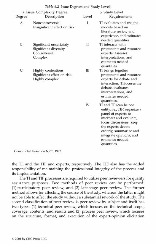
the TI, and the TIF and experts, respectively. The TIF also has the addedresponsibility of maintaining the professional integrity of the process andits implementation.
The TI and TIF processes are required to utilize peer reviewers for qualityassurance purposes. Two methods of peer review can be performed:(1) participatory peer review, and (2) late-stage peer review. The formermethod allows for affecting the course of the study, whereas the latter mightnot be able to affect the study without a substantial rework of the study. Thesecond classification of peer review is peer-review by subject and itself hastwo types: (1) technical peer review, which focuses on the technical scope,coverage, contents, and results and (2) process peer review, which focuseson the structure, format, and execution of the expert-opinion elicitation
Table 6.2 Issue Degrees and Study Levels
a. Issue Complexity Degree b. Study LevelDegree Description Level Requirements
A NoncontroversialInsignificant effect on risk
I TI evaluates and weighs models based on literature review and experience, and estimates needed quantities.
B Significant uncertaintySignificant diversityControversialComplex
II TI interacts with proponents and resource experts, assesses interpretations, and estimates needed quantities.
C Highly contentiousSignificant effect on riskHighly complex
III TI brings together proponents and resource experts for debate and interaction. TI focuses the debate, evaluates interpretations, and estimates needed quantities.
IV TI and TF (can be one entity, i.e., TIF) organize a panel of experts to interpret and evaluate, focus discussions, keep the experts debate orderly, summarize and integrate opinions, and estimates needed quantities.
Constructed based on NRC, 1997
© 2001 by CRC Press LLC
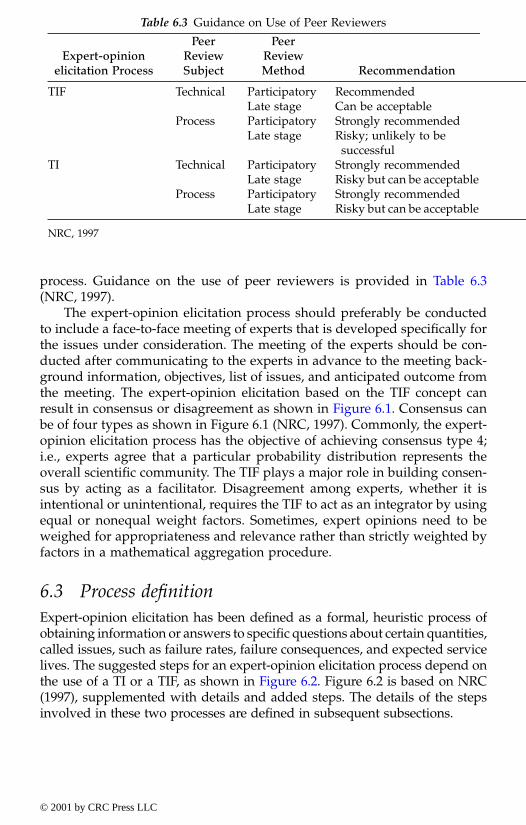
process. Guidance on the use of peer reviewers is provided in Table 6.3(NRC, 1997).
The expert-opinion elicitation process should preferably be conductedto include a face-to-face meeting of experts that is developed specifically forthe issues under consideration. The meeting of the experts should be con-ducted after communicating to the experts in advance to the meeting back-ground information, objectives, list of issues, and anticipated outcome fromthe meeting. The expert-opinion elicitation based on the TIF concept canresult in consensus or disagreement as shown in Figure 6.1. Consensus canbe of four types as shown in Figure 6.1 (NRC, 1997). Commonly, the expert-opinion elicitation process has the objective of achieving consensus type 4;i.e., experts agree that a particular probability distribution represents theoverall scientific community. The TIF plays a major role in building consen-sus by acting as a facilitator. Disagreement among experts, whether it isintentional or unintentional, requires the TIF to act as an integrator by usingequal or nonequal weight factors. Sometimes, expert opinions need to beweighed for appropriateness and relevance rather than strictly weighted byfactors in a mathematical aggregation procedure.
6.3 Process definitionExpert-opinion elicitation has been defined as a formal, heuristic process ofobtaining information or answers to specific questions about certain quantities,called issues, such as failure rates, failure consequences, and expected servicelives. The suggested steps for an expert-opinion elicitation process depend onthe use of a TI or a TIF, as shown in Figure 6.2. Figure 6.2 is based on NRC(1997), supplemented with details and added steps. The details of the stepsinvolved in these two processes are defined in subsequent subsections.
Table 6.3 Guidance on Use of Peer Reviewers
Expert-opinionelicitation Process
Peer Review Subject
PeerReview Method Recommendation
TIF Technical Participatory RecommendedLate stage Can be acceptable
Process Participatory Strongly recommendedLate stage Risky; unlikely to be
successfulTI Technical Participatory Strongly recommended
Late stage Risky but can be acceptableProcess Participatory Strongly recommended
Late stage Risky but can be acceptable
NRC, 1997
© 2001 by CRC Press LLC
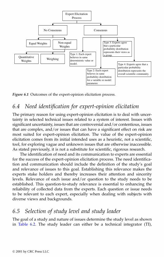
6.4 Need identification for expert-opinion elicitationThe primary reason for using expert-opinion elicitation is to deal with uncer-tainty in selected technical issues related to a system of interest. Issues withsignificant uncertainty, issues that are controversial and/or contentious, issuesthat are complex, and/or issues that can have a significant effect on risk aremost suited for expert-opinion elicitation. The value of the expert-opinionelicitation comes from its initial intended uses as a heuristic, not a scientific,tool, for exploring vague and unknown issues that are otherwise inaccessible.As stated previously, it is not a substitute for scientific, rigorous research.
The identification of need and its communication to experts are essentialfor the success of the expert-opinion elicitation process. The need identifica-tion and communication should include the definition of the study’s goaland relevance of issues to this goal. Establishing this relevance makes theexperts stake holders and thereby increases their attention and sinceritylevels. Relevance of each issue and/or question to the study needs to beestablished. This question-to-study relevance is essential to enhancing thereliability of collected data from the experts. Each question or issue needsto be relevant to each expert, especially when dealing with subjects withdiverse views and backgrounds.
6.5 Selection of study level and study leader The goal of a study and nature of issues determine the study level as shownin Table 6.2. The study leader can either be a technical integrator (TI),
Figure 6.1 Outcomes of the expert-opinion elicitation process.
Expert ElicitationProcess
ConsensusNo Consensus
Equal Weights Non-equalWeights
QuantitativeWeights
Weighing
Type 1: Each expertbelieves in samedeterministic value ormodel.
Type 2: Each expertbelieves in sameprobability distributionfor a variable or modelparameter.
Type 3: Experts agreethat a particularprobability distributionrepresents their views asa group.
Type 4: Experts agree that aparticular probabilitydistribution represents theoverall scientific community.
© 2001 by CRC Press LLC
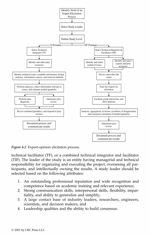
technical facilitator (TF), or a combined technical integrator and facilitator(TIF). The leader of the study is an entity having managerial and technicalresponsibility for organizing and executing the project, overseeing all par-ticipants, and intellectually owning the results. A study leader should beselected based on the following attributes:
1. An outstanding professional reputation and wide recognition andcompetence based on academic training and relevant experience;
2. Strong communication skills, interpersonal skills, flexibility, impar-tiality, and ability to generalize and simplify;
3. A large contact base of industry leaders, researchers, engineers,scientists, and decision makers; and
4. Leadership qualities and the ability to build consensus.
Figure 6.2 Expert-opinion elicitation process.
Identify Need of anExpert Elicitation
Process
Define Study Level
Select TechnicalIntegrator (TI)
TIF ProcessTI Process
Select Study Leader
Identify and select peerreviewers
Identify technical issues, available information, designanalyses, information sources, and retrieval methods
Perform analyses, collect information relevant toissues, and estimate needed quantities
Perform datadiagnostic
Administer peerreview
Revise estimated quantities, and respond to peerreviews
Select Technical Integrator &Facilitator (TIF)
Discuss and refine theissues
Train the experts forelicitation
Facilitate group interaction, andelicit opinions
Analysis, aggregation, revisions, resolution of disagreement,and consensus estimation of needed quantities
Document process andcommunicate results
Document process andcommunicate results
Identify and selecttechnical issues
Identify and selectexperts and peer
reviewers
Administer peerreview
© 2001 by CRC Press LLC
The study leader does not need to be a subject expert, but should beknowledgeable of the subject matter.
6.6 Selection of peer reviewers and experts6.6.1 Selection of peer reviewers
Peer review can be classified according to the peer-review method andaccording to the peer-review subject. There are two methods of peer review:(1) participatory peer review which is conducted as an ongoing reviewthroughout all study stages, and (2) late-stage peer review which is per-formed as the final stage of the study. Peer-review subject also has two types:(1) technical peer review and (2) process peer review. These classificationswere discussed in Section 6.2.
Peer reviewers are needed for both the TI and TIF processes and shouldbe selected by the study leader in close consultation with perhaps the studysponsor. Researchers, engineers, and scientists with the following character-istics should be sought as peer reviewers:
• Outstanding professional reputation, and widely recognized compe-tence based on academic training and relevant experience,
• General understanding of the issues in other related areas and/orwith relevant expertise and experiences from other areas,
• Available and willing to devote the needed time and effort, and• Strong communication skills, interpersonal skills, flexibility, impar-
tiality, and ability to generalize and simplify.
6.6.2 Identification and selection of experts
The size of an expert panel should be determined on a case-by-case basis.The panel should be large enough to achieve a needed diversity of opinion,credibility, and result reliability. In recent expert-opinion elicitation studies,a nomination process was used to establish a list of candidate experts byconsulting archival literature, technical societies, governmental organiza-tions, and other knowledgeable experts (Trauth et al., 1993). Formal nomi-nation and selection processes should establish appropriate criteria for nom-ination, selection, and removal of experts. For example, these criteria wereused in an ongoing Yucca Mountain seismic hazard analysis (NRC, 1997) toselect experts:
1. Strong relevant expertise through academic training, professionalaccomplishment and experiences, and peer-reviewed publications;
2. Familiarity and knowledge of various aspects related to the issues ofinterest;
3. Willingness to act as proponents or impartial evaluators;
© 2001 by CRC Press LLC

4. Availability and willingness to commit needed time and effort;5. Specific related knowledge and expertise of the issues of interest;6. Willingness to effectively participate in needed debates, to prepare
for discussions, and provide needed evaluations and interpretations;and
7. Strong communication skills, interpersonal skills, flexibility, impar-tiality, and ability to generalize and simplify.
In this NRC study, criteria for removing experts included failure toperform according to commitments and demands as set in the selectioncriteria, and unwillingness to interact with members of the study.
The panel of experts for an expert-opinion elicitation process shouldhave a balance and broad spectrum of viewpoints, expertise, technical pointsof view, and organizational representation. The diversity and completenessof the panel of experts is essential for the success of the elicitation process.For example, it can include the following:
1. Proponents who advocate a particular hypothesis or technicalposition;
2. Evaluators who consider available data, become familiar with theviews of proponents and other evaluators, question the technicalbases of data, and challenge the views of proponents; and
3. Resource experts who are technical experts with detailed and deepknowledge of particular data, issue aspects, particular methodolo-gies, or use of evaluators.
The experts should be familiar with the design, construction, opera-tional, inspection, maintenance, reliability, and engineering aspects of theequipment and components of a facility of interest. For this study, it wasessential to select people with basic engineering or technological knowledge;however they do not necessarily need to be engineers. It might be necessaryto include one or two experts from management with engineering knowl-edge of the equipment and components, consequences, safety aspects,administrative and logistic aspects of operation, expert-opinion elicitationprocess, and objectives of this study. One or two experts with a broaderknowledge of the equipment and components might be needed. Also, oneor two experts with a background in risk analysis and risk-based decisionmaking and their uses in areas related to the facility of interest might beneeded.
Observers can be invited to participate in the elicitation process and cancontribute to the discussion, but they cannot provide expert opinion thatenters in the aggregated opinion of the experts. The observers provide exper-tise in the elicitation process, probabilistic and statistical analyses, risk anal-ysis, and other support areas. The composition and contribution of theobservers are essential for the success of this process. The observers mayinclude the following:
© 2001 by CRC Press LLC
• Individuals with research or administrative-related background fromresearch laboratories or headquarters of the U.S. Army Corps ofEngineers with engineering knowledge of equipment and compo-nents of Corps facilities.
• Individuals with expertise in probabilistic analysis, probabilisticcomputations, consequence computations and assessment, and ex-pert-opinion elicitation.
A list of names with biographical statements of the study leader, tech-nical integrator, technical facilitator, experts, observers, and peer reviewersshould be developed. All attendees can participate in the discussions duringthe meeting. However, only the experts can provide the needed answers toquestions on the selected issues. The integrators and facilitators are respon-sible for conducting the expert-opinion elicitation process. They can be con-sidered to be a part of the observers or experts depending on the circum-stances and the needs of the process.
6.6.3 Items needed by experts and reviewers before the expert-opinion elicitation meeting
The experts and observers need to receive the following items before theexpert-opinion elicitation meeting:
• An objective statement of the study;• A list of experts, observers, integrators, facilitators, study leader,
sponsors, and their biographical statements;• A description of the facility, systems, equipment, and components;• Basic terminology and definitions that may include probability, fail-
ure rate, average time between unsatisfactory performances, mean(or average) value, median value, and uncertainty;
• Failure consequence estimation;• A description of the expert-opinion elicitation process;• A related example of the expert-opinion elicitation process and its
results, if available;• Aggregation methods of expert opinions, such as computations of
percentiles;• A description of the issues in the form of a list of questions with
background descriptions. Each issue should be presented on a sep-arate page with spaces for recording an expert’s judgment, any revi-sions and comments. Clear statements of expectations from the ex-perts in terms of time, effort, responses, communication, anddiscussion style and format.
It might be necessary to personally contact individual experts for thepurpose of establishing clear understanding of expectations.
© 2001 by CRC Press LLC
6.7 Identification, selection and development of technical issues
The technical issues of interest should be carefully selected to achieve certainobjectives. In these guidelines, the technical issues are related to the quan-titative assessment of failure probabilities and consequences for selectedcomponents, subsystems, and systems within a facility. The issues shouldbe selected such that they would have a significant impact on the studyresults. These issues should be structured in a logical sequence, starting withbackground statement, followed by questions, and then answer selectionsor answer format and scales. Personnel with risk-analysis background whoare familiar with the construction, design, operation, and maintenance of thefacility need to define these issues in the form of specific questions. Also,background materials about these issues need to be assembled. The materialswill be used to familiarize and train the experts about the issues of interestas described subsequent steps.
An introductory statement for the expert-opinion elicitation processshould be developed that includes the goal of the study and establishesrelevance. Instructions should be provided with guidance on expectations,answering questions, and reporting. The following are guidelines on con-structing questions and issues based on social research practices (Bailey,1994):
1. Each issue can include several questions; however, each questionshould elicit only one opinion. It is a poor practice to include twoquestions in one.
2. Question and issue statements should not be ambiguous. Also, theuse of ambiguous words should be avoided. In expert-opinion elic-itation of failure probabilities, the word “failure” might be vague orambiguous to some subjects. Special attention should be given to itsdefinition within the context of each issue or question. The level ofwording should be kept to a minimum. Also, word choice mightaffect the connotation of an issue.
3. The use of factual questions is preferred over abstract questions.Questions that refer to concrete and specific matters result in concreteand specific answers which is what is wanted.
4. Questions should be carefully structured in order to reduce biases ofsubjects. Questions should be asked in a neutral format; sometimesit is more appropriate not to have lead statements.
5. Sensitive topics might require stating questions with lead statementsto establish supposedly accepted social norms in order to encouragesubjects to answers the questions truthfully.
Questions can be classified into open-ended questions and closed-endedquestions as previously discussed. The format of the question should be
© 2001 by CRC Press LLC
selected carefully. The format, scale, and units for the response categoriesshould be selected to best achieve the goal of the study. The question orderand minimum number of questions should be selected, using the guidelinesof Section 3.8.
Once the issues are developed, they should be pretested by administer-ing them to a few subjects for the purpose of identifying and correctingflaws. The results of this pretesting should be used to revise the issues.
6.8 Elicitation of opinionsThe elicitation of opinions process should be systematic for all the issues,according to the steps presented in this section.
6.8.1 Issue familiarization of experts
The background materials that were assembled in the previous step shouldbe sent to the experts one to two weeks in advance of the meeting to providesufficient time for them to become familiar with the issues. The objective ofthis step is also to ensure that there is a common understanding among theexperts of the issues. The background material should include the objectivesof the study, description of the issues, lists of questions for the issues, descrip-tion of systems and processes, their equipment and components, the descrip-tion of elicitation process and of the method for selecting experts, and bio-graphical information on the selected experts. Also, example results and theirmeaning, methods of analysis of the results, and lessons learned from pre-vious elicitation processes should be made available. It is important to breakthe questions or issues into components that can be easily addressed. Pre-liminary discussion meetings or telephone conversations between the facil-itator and experts might be necessary in some cases in preparation for theelicitation process.
6.8.2 Training of experts
Expert training is performed during the meeting of the experts, observers,and facilitators. During the training, the facilitator needs to remain flexibleto refining wording or even changing the approach based on feedback fromexperts. For instance, experts might not be comfortable with the term “prob-ability” but may answer about “events per year” or “recurrence interval.”This indirect elicitation, as discussed in Section 3.6.1, should be exploredwith the experts.
The meeting should be started with presentations of background mate-rial to establish relevance of the study to the experts and study goals in orderto establish rapport with the experts. Then, information on uncertaintysources and types, occurrence probabilities and consequences, the expert-opinion elicitation process, technical issues and questions, and aggregation
© 2001 by CRC Press LLC
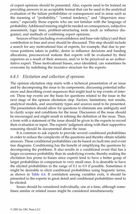
of expert opinions should be presented. Also, experts need to be trained onproviding answers in an acceptable format that can be used in the analyticalevaluation of the failure probabilities or consequences and in areas such asthe meaning of “probability,” “central tendency,” and “dispersion mea-sures,” especially those experts who are not familiar with the language ofprobability. Additional training might be needed on consequences, subjectiveassessment, logic trees, problem-structuring tools (such as influence dia-grams), and methods of combining expert opinions.
Sources of bias (including overconfidence and base-rate fallacy) and theircontribution to bias and error should be discussed. This step should includea search for any motivational bias of experts, for example, that due to pre-vious positions taken in public, desire to influence decisions and fundingallocations, preconceived notions that experts will be evaluated by theirsuperiors as a result of their answers, and/or to be perceived as an author-itative expert. These motivational biases, once identified, can sometimes beovercome by redefining the incentive structure for the experts.
6.8.3 Elicitation and collection of opinions
The opinion elicitation step starts with a technical presentation of an issueand by decomposing the issue to its components, discussing potential influ-ences and describing event sequences that might lead to top events of inter-est. These top events are the basis for questions related to the issue in thenext stage of the opinion elicitation step. Factors, limitations, test results,analytical models, and uncertainty types and sources need to be presented.The presentation should allow for questions to eliminate any ambiguity andto clarify scope and conditions for the issue. Discussion of the issue shouldbe encouraged and might result in refining the definition of the issue. Then,a form with a statement of the issue should be given to the experts to recordtheir evaluation or input. The experts’ judgment along with their supportivereasoning should be documented about the issue.
It is common to ask experts to provide several conditional probabilitiesin order to reduce the complexity of the questions and thereby obtain reliableanswers. These conditional probabilities can be based on fault tree and eventtree diagrams. Conditioning has the benefit of simplifying the questions bydecomposing the problems. It also results in a conditional event that has alarger occurrence probability than its underlying events; thereby making theelicitation less prone to biases since experts tend to have a better grasp oflarger probabilities in comparison to very small ones. It is desirable to havethe elicited probabilities in the range of 0.1 to 0.9 if possible. Sometimes itmight be desirable to elicit conditional probabilities using linguistic terms,as shown in Table 4.6. If correlation among variables exits, it should bepresented to the experts in great detail and conditional probabilities need tobe elicited.
Issues should be considered individually, one at a time, although some-times similar or related issues might be considered simultaneously.
© 2001 by CRC Press LLC
6.8.4 Aggregation and presentation of results
The collected assessments from the experts for an issue should be assessedfor internal consistency, analyzed, and aggregated to obtain compositejudgments for the issue. The means, medians, percentile values, and stan-dard deviations need to be computed for the issues. Also, a summary ofthe reasoning provided during the meeting about the issues needs to bedeveloped. Uncertainty levels in the assessments should also be quantified.Methods for combining expert opinions are provided in Chapter 5. Themethods can be classified into consensus methods and mathematical meth-ods. The mathematical methods can be based on assigning equal weightsor different weights to the experts.
6.8.5 Group interaction, discussion, and revision by experts
The aggregated results need to be presented to the experts for a second roundof discussion and revision. The experts should be given the opportunity torevise their assessments of the individual issues at the end of discussion.Also, they should be asked to state the rationale for their statements andrevisions. The revised assessments of the experts need to be collected foraggregation and analysis. This step can produce either consensus or noconsensus as shown in Figure 6.1. The selected aggregation procedure mightrequire eliciting weight factors from the experts. In this step the technicalfacilitator plays a major role in developing a consensus, and maintaining theintegrity and credibility of the elicitation process. Also, the technical inte-grator is needed to aggregate the results without biases with reliabilitymeasures. The integrator might need to deal with varying expertise levelsfor the experts, outliers (i.e., extreme views), nonindependent experts, andexpert biases.
6.9 Documentation and communicationA comprehensive documentation of the process is essential in order to ensureacceptance and credibility of the results. The document should include com-plete descriptions of the steps, the initial results, revised results, consensusresults, and aggregated results spreads and reliability measures.
6.10 Exercise problemsProblem 6.1 What are the differences between the technical facilitator, andtechnical integrator, and facilitator in an expert-opinion elicitation process?
Problem 6.2 What are the success requirements for selecting experts anddeveloping an expert panel? How many experts would you recommend?For your range on the number of experts, provide guidance in using thelower and upper ends of the range.
© 2001 by CRC Press LLC

Problem 6.3 Working in teams, select five classmates as a panel of expertsand elicit their opinions on five forecasting issues in engineering. Select theseissues such that the classmates can pass the test of experts on these issues.Perform all the steps of expert-opinion elicitation; document your processand results as a part of solving this problem.
© 2001 by CRC Press LLC

chapter seven
Applications of expert-opinion elicitation
Contents
7.1. Introduction7.2. Assessment of occurrence probabilities
7.2.1. Cargo elevators onboard ships7.2.1.1. Background7.2.1.2. Example issues and results
7.2.2. Navigation locks7.2.2.1. Background7.2.2.2. General description of lock operations7.2.2.3. Description of components7.2.2.4. Example issues and results
7.3. Economic consequences of floods7.3.1. Background7.3.2. The Feather River basin
7.3.2.1. Levee failure and consequent flooding7.3.2.2. Flood characteristics7.3.2.3. Building characteristics7.3.2.4. Vehicle characteristics
7.3.3. Example issues and results7.3.3.1. Structural depth-damage relationships7.3.3.2. Content depth-damage relationships7.3.3.3. Content-to-structure value ratios7.3.3.4. Vehicle depth-damage relationship
7.1 IntroductionThis chapter demonstrates the application of expert-opinion elicitation byfocusing on occurrence probabilities and consequences of events related tonaval and civil works systems for the purposes of planners, engineers, and
© 2001 by CRC Press LLC

others, should they choose to use expert judgment. For this purpose, formalprocesses of obtaining information or answers to specific questions aboutcertain quantities, called issues, such as failure rates and probabilities, andfailure consequences were conducted, and opinions were elicited and ana-lyzed as presented in this chapter. The guidance on expert-opinion elicitationof Chapter 6 was used for this purpose. The chapter is divided into sectionsthat deal with using expert-opinion elicitation in assessing failure probabil-ities and failure consequences.
7.2 Assessment of occurrence probabilities7.2.1 Cargo elevators onboard ships
7.2.1.1 BackgroundThis example illustrates the use of expert-opinion elicitation to obtain failureprobabilities needed to study the safety of cargo elevators onboard navalships (Ayyub, 1992). In order to study the safety of the elevators and theeffect of add-on safety features, a fault tree analysis was performed. Thefault tree analysis requires the knowledge of failure probabilities of basicevents, such as the unsatisfactory performance of mechanical or electricalcomponents and human errors.
Generally, the failure probabilities can be obtained from several sources,such as failure records, failure databases, literature review, or industry-basedreports and documents. However, in some cases these sources do not containthe needed probabilities for some basic events. In such cases, expert-opinionelicitation can be used to obtain the needed information. For example, thefailure rate of the hoisting machinery brake was obtained from failurerecords, and the probability that a passerby would fall into an open elevatortrunk (human error) required expert-opinion elicitation.
In the elevator safety study, about 250 issues were identified for theexpert-opinion elicitation process. The issues were presented to the expertswith the needed background information over a three-day period. All theissues were discussed and addressed in this time period.
This section provides example issues and results of expert-opinion elic-itation. Since the background information on the types of elevators and theiruse and limitation are not provided in this section, the results reported hereincan be considered to be hypothetical and should not be used for otherpurposes.
7.2.1.2 Example issues and resultsTwo example issues are described in this section:
1. How often does the load on a platform shift as a result of being poorlystacked?
© 2001 by CRC Press LLC

2. During one loading revolution at one deck level, what is the proba-bility that a fork truck driver will place the load such that it overhangsthe edge of the platform?
Eight experts were used in the expert-opinion elicitation process. Theresults of the process were summarized in the form of percentiles. Thepercentiles were computed using the equations in Table 4.7. Tables 7.1 and 7.2summarize the results of the expert-opinion elicitation for issues 1 and 2,respectively. The results are expressed as the number of unsatisfactory per-formances per year and a percent for issues 1 and 2, respectively. Theseresults were used to compute the needed probabilities in the fault tree anal-ysis. It is desirable in expert-opinion elicitation to state the issues in the mostsuitable form and units in order to obtain the best results from the experts.
7.2.2 Navigation locks
7.2.2.1 BackgroundDetailed descriptions of technical issues are essential for the success of anexpert-opinion elicitation process and need to be provided to the experts.The descriptions should provide the experts of background materials, clearstatements of issues, objectives, formats, and opinion aggregation that wouldbe used in elicitation sessions. In this example, a description of a navigationlock and fault scenarios are presented for demonstration purposes. Theequipment and components are based on the Emsworth navigation lock onthe Ohio River. Ayyub et al. (1996) used technical background materials onthe operations of the lock to develop relevant technical issues.
A navigation lock can be considered to constitute a system that consistsof equipment which consists of components consisting of elements. Theequipment, components, and elements are called the levels of analysis. Inestimating failure likelihood and consequences, decisions need to be madeon the level of computations for an item in the process, i.e., equipment,component, or element level. The decision can be based on the availabilityof information, the logistic of inspection that might define the entity or unit,the objectives of risk analyses performed on the lock, or other considerations.Accordingly, the level of computations does not need to be the same for allitems within the process.
7.2.2.2 General description of lock operationsThe operation of the lock is shown in the logic diagram in Figures 7.1a and7.2b (Ayyub et al., 1996).
The lock consists of two adjacent, parallel lock chambers located alongthe right bank of the main channel. The large lock chamber occupies thelandward position and has clear dimensions of 110 ft × 600 ft. The smallerriver chamber measures 56 ft × 360 ft. Normal lift is 18 feet. The lock wallsand sills are the gravity type and founded on rock. Both the upper and lower
© 2001 by CRC Press LLC

Table 7.1 Expert-Opinion Elicitation for Example Issue 1
Event Name Full Description
Expert-opinion elicitation(8 experts) Summary
FirstResponse Median
SecondResponse Median
Load is poorlystacked.
The load on the platform is stacked in such a manner that it is shifted by normal starting and stopping of the platform. Assume that the ship is in calm sea state.
Issue:
On one elevator, how often does the load on the platform shift as a result of being poorly stacked?
Issue:
1 in 1 yr1 in 1 yr1 in 0.5 yr1 in 2 yrs1 in 0.1 yr1 in 1 yr1 in 0.1 yr1 in 15 yr
1 in 1 yr
Issue:
1 in 1 yr1 in 1 yr1 in 0.5 yr1 in 1 yr1 in 0.5 yr1 in 1 yr1 in 0.5 yr1 in 1 yr
1 in 1 yr
Low1 in 1 year25 percentile1 in 1 yearMedian1 in 1 year75 percentile1 in 0.5 yearHigh1 in 0.5 year
Ayyub, 1992; Ayyub et al., 1996
© 2001 by C
RC
Press LL
C

Table 7.2 Expert-Opinion Elicitation for Example Issue 2
Event Name Full Description
Expert-opinion elicitation(8 experts) Summary
FirstResponse Median
SecondResponse Median
Fork truck driverplacesloadover-hangingplatform.
Fork truck driver places load such that it overhangs platform despite the existence of adequate lighting. Assume that there are no yellow margins painted on the platform.
Issue:
During one loading evolution at one deck level, what is the probability that a fork truck driver will place the load such that it overhangs the edge of the platform?
Issue:
1%1%10%0.1%0.5%1%0.5%0.5%
0.75%
Issue:
1%1%10%1%0.5%1%0.5%0.5%
1%
Low0.5%25 percentile0.5%Median1%75 percentile1%High10%
Ayyub, 1992; Ayyub et al., 1996
© 2001 by C
RC
Press LL
C
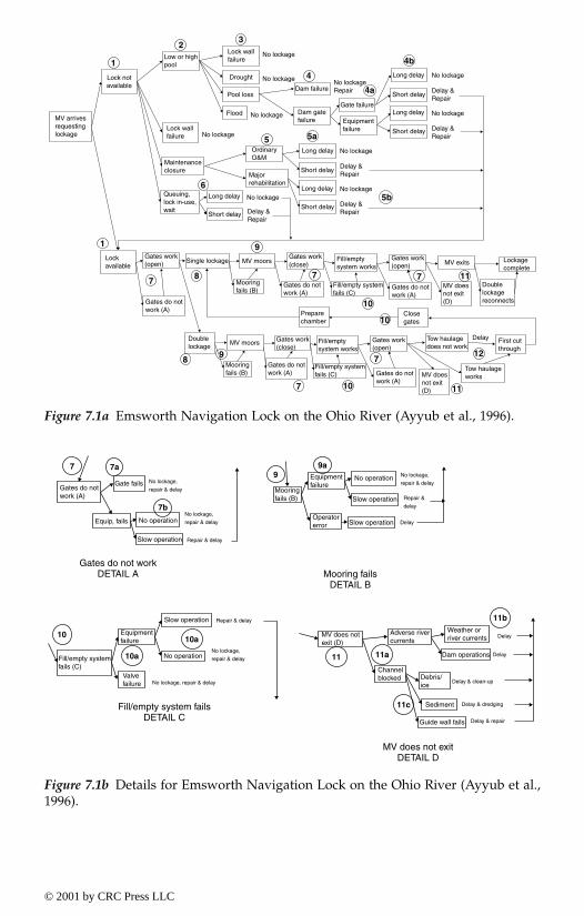
Figure 7.1a Emsworth Navigation Lock on the Ohio River (Ayyub et al., 1996).
Figure 7.1b Details for Emsworth Navigation Lock on the Ohio River (Ayyub et al.,1996).
1
23
4
5
6
1
7 8
9
7
10
10
10 11
12
7
7
7
98
11
5a
5b
4a
4b
Lock notavailable
Low or highpool
No lockage
No lockage
No lockage
No lockage
No lockage
Flood
Pool loss
Drought
Lock wallfailure
Dam failure
Dam gatefailure
No lockageRepair
Gate failure
Equipmentfailure
No lockage
No lockage
Long delay
Long delayLong delay
Short delay
Short delay
Short delay
Lock wallfailure
OrdinaryO&M
Majorrehabilitation
Maintenanceclosure
Queuing,lock in-use,wait Delay &
Repair
MV arrivesrequestinglockage
Delay &Repair
Delay &Repair
No lockage
No lockage
Long delay
Long delay
Short delay
Short delay
Delay &Repair
Delay &Repair
Lockavailable
Gates work(open) Single lockage MV moors
Mooringfails (B)
Gates do notwork (A)
Gates do notwork (A) Gates do not
work (A)
Gates do notwork (A)
Gates do notwork (A)
Gates work(close)
Fill/emptysystem works
Fill/empty systemfails (C)
Fill/empty systemfails (C)
Gates work(open) MV exits
Preparechamber
Closegates
MV doesnot exit(D)
Lockagecomplete
Doublelockagereconnects
Delay First cutthrough
Tow haulagedoes not work
Tow haulageworks
Gates work(open)
Fill/emptysystem works
Gates work(close)
MV moors
Mooringfails (B)
Doublelockage
MV doesnot exit(D)
Gates do notwork (A)
Gate fails No lockage,
repair & delay
Equip, fails No operation
Slow operation
No lockage,
repair & delay
Repair & delay
7 7a
7b
10
10a
10a
99a
11 11a
11c
11b
Fill/empty systemfails (C)
Valvefailure No lockage, repair & delay
Equipmentfailure
Slow operation
No operation
Repair & delay
No lockage,
repair & delay
Mooringfails (B)
Equipmentfailure
Operatorerror
No operation
Slow operation
Slow operation Delay
Repair &
delay
No lockage,
repair & delay
MV does notexit (D)
Channelblocked Debris/
ice
Adverse rivercurrents
Weather orriver currents
Dam operations Delay
Delay
Delay & clean-up
Sediment Delay & dredging
Delay & repairGuide wall fails
Gates do not workDETAIL A
Fill/empty system failsDETAIL C
MV does not exitDETAIL D
Mooring failsDETAIL B
© 2001 by CRC Press LLC

guide and guard walls are concrete gravity sections, but the upper and lowerguard walls have been extended using steel sheet pile cells. The filling andemptying of the lock chambers is accomplished through ports in the middleand river walls. The large chamber is filled by 16 cylindrical valves locatedin the upper end of the middle wall and emptied by 16 similar valves whichpass the water through a culvert under the smaller chamber and into theriver below the dam. A supplemental filling system was instituted during arecent major rehabilitation and involved the reopening of a 10-ft diameterturbine tunnel, providing a slide gate, plugging the tailrace exit, and cuttingfilling ports through the land wall at lock floor level. The small chamberuses only six filling and six emptying valves in the river wall. The lock gatesare of the mitering type, hinged to embedded anchorages at the top andsupported at the bottom on steel pintles. Each leaf is a rectangular framewith vertical girders at each end, and vertical beams and horizontal inter-costals on the gate leaves for the 110-ft chamber, or horizontal beams andvertical intercostals on the leaves for the 56-ft chamber. Upstream closure ofthe large chamber is accomplished using trestles stored underwater that areraised from notches in a concrete sill upstream of the miter gates and thenfitted with bulkheads. The small chamber uses a coffer beam and needletype closure. Downstream closure for both chambers is accomplished withpoiree dams. The average number of annual lockages has remained fairlyconstant over the last 30 years at about 9950, with commercial lockagesdecreasing and recreational lockages increasing in recent years.
7.2.2.3 Description of componentsAs a system, the Emsworth navigation lock on the Ohio River consists ofgates, dam, walls, channel, equipment, and users. The following are descrip-tions of its components:
1. Filling and emptying valves: The filling and emptying of the lockchambers are accomplished through culverts placed in the middleand river walls. The main lock is filled by 16 cylindrical valves locatedin the upper end of the middle wall and emptied by 16 similar valveswhich pass the water through the lower end of the wall and underthe riverward chamber into the river below the dam.
2. Filling and emptying equipment: The hydraulic system consists ofthree constant delivery oil pumps and one pressure-holding oilpump, located on the first floor in the operation building on the landwall. The pumps supply oil under pressure to the hydraulic pipingsystem for operation of the lock gate and culvert valve operatingmachinery on the lock walls. This system was installed in 1968 andreplaced the original compressed air system for operation of the mitergates and the original hydraulic system installed for operation of theemptying and filling valves.
© 2001 by CRC Press LLC

3. Lock wall: The lock walls are the gravity type founded on rock. Widthof the wall at the top is 5 ft minimum and 24 ft maximum. The sillsare concrete gravity sections and anchor rods are installed wherecomputations indicated their need.
4. Guide wall: The upper guide wall is 1023.19 ft long measured fromthe upstream nose of the middle wall, and the lower guide wall is650.0 ft long measured from the downstream nose of the middle wall.They are gravity structures founded on rock, except for the upperguide wall extension which is constructed of individual steel sheetpile cells.
5. Miter gates: The lock gates are constructed of structural steel shapesand plates. The gate leaves for the 110-ft chamber are verticallyframed. Each gate consists of two leaves that are hinged to embeddedanchorages at the top by gudgeon pins and are supported at thebottom on steel pintles, with the pintle bases embedded in concrete.Each leaf is a rectangular frame with vertical quoin and miter girdersat the fixed and free ends, respectively, and vertical beams and hor-izontal intercostals on the gate leaves for the 110-ft chamber.
6. Miter gate-operating equipment: The hydraulic system consists ofthree constant delivery oil pumps and one pressure holding oilpump, located on the first floor in the operation building on the landwall. The pumps supply oil under pressure to the hydraulic pipingsystem for operation of the lock gate and culvert valve operatingmachinery on the lock walls. This system was installed in 1968 andreplaced the original compressed air system for operation of the mitergates and the original hydraulic system installed for operation of theemptying and filling valves.
7. Dam gates: The 13 submergible lift gates are steel structures arrangedto travel on vertical tracks on the piers. Each gate can be raised to apoint where its bottom is 39.4 ft above the sill and lowered to a pointwhere its top is 3 ft below normal pool level. There is one Sidneygate located on the back channel dam. This gate combines featuresof both the tainter and vertical lift gates. The gate works like a taintergate until the gate reaches the limits of its rotation, after which theentire gate is raised by the lifting chains up to the maximum travellimit, 38 ft above the sill.
8. Dam gate-operating equipment: Two hoist motors and two synchro-nous tie motors of the slip-ring induction type are provided for eachgate. A full magnetic reverse control panel operates the two hoistmotors and the two synchronous tie motors for each gate from aremotely mounted master switch. In the case of emergency, eitherhoisting motor may be cut out by means of switches, and the gatecan be operated by the remaining motor through the synchronoustie motors.
© 2001 by CRC Press LLC
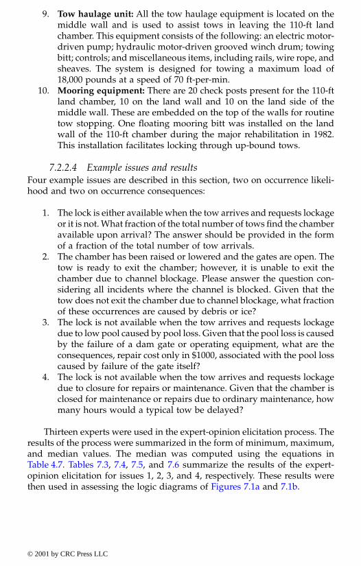
9. Tow haulage unit: All the tow haulage equipment is located on themiddle wall and is used to assist tows in leaving the 110-ft landchamber. This equipment consists of the following: an electric motor-driven pump; hydraulic motor-driven grooved winch drum; towingbitt; controls; and miscellaneous items, including rails, wire rope, andsheaves. The system is designed for towing a maximum load of18,000 pounds at a speed of 70 ft-per-min.
10. Mooring equipment: There are 20 check posts present for the 110-ftland chamber, 10 on the land wall and 10 on the land side of themiddle wall. These are embedded on the top of the walls for routinetow stopping. One floating mooring bitt was installed on the landwall of the 110-ft chamber during the major rehabilitation in 1982.This installation facilitates locking through up-bound tows.
7.2.2.4 Example issues and resultsFour example issues are described in this section, two on occurrence likeli-hood and two on occurrence consequences:
1. The lock is either available when the tow arrives and requests lockageor it is not. What fraction of the total number of tows find the chamberavailable upon arrival? The answer should be provided in the formof a fraction of the total number of tow arrivals.
2. The chamber has been raised or lowered and the gates are open. Thetow is ready to exit the chamber; however, it is unable to exit thechamber due to channel blockage. Please answer the question con-sidering all incidents where the channel is blocked. Given that thetow does not exit the chamber due to channel blockage, what fractionof these occurrences are caused by debris or ice?
3. The lock is not available when the tow arrives and requests lockagedue to low pool caused by pool loss. Given that the pool loss is causedby the failure of a dam gate or operating equipment, what are theconsequences, repair cost only in $1000, associated with the pool losscaused by failure of the gate itself?
4. The lock is not available when the tow arrives and requests lockagedue to closure for repairs or maintenance. Given that the chamber isclosed for maintenance or repairs due to ordinary maintenance, howmany hours would a typical tow be delayed?
Thirteen experts were used in the expert-opinion elicitation process. Theresults of the process were summarized in the form of minimum, maximum,and median values. The median was computed using the equations inTable 4.7. Tables 7.3, 7.4, 7.5, and 7.6 summarize the results of the expert-opinion elicitation for issues 1, 2, 3, and 4, respectively. These results werethen used in assessing the logic diagrams of Figures 7.1a and 7.1b.
© 2001 by CRC Press LLC
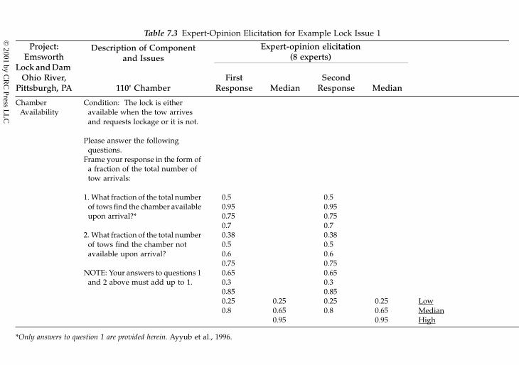
Table 7.3 Expert-Opinion Elicitation for Example Lock Issue 1
Project:Emsworth
Lock and Dam Ohio River,
Pittsburgh, PA
Description of Componentand Issues
Expert-opinion elicitation(8 experts)
110' ChamberFirst
Response MedianSecond
Response Median
ChamberAvailability
Condition: The lock is either available when the tow arrives and requests lockage or it is not.
Please answer the following questions.
Frame your response in the form of a fraction of the total number of tow arrivals:
1. What fraction of the total number of tows find the chamber available upon arrival?*
2. What fraction of the total number of tows find the chamber not available upon arrival?
NOTE: Your answers to questions 1 and 2 above must add up to 1.
0.50.950.750.70.380.50.60.750.650.30.850.250.8
0.250.650.95
0.50.950.750.70.380.50.60.750.650.30.850.250.8
0.250.650.95
LowMedianHigh
*Only answers to question 1 are provided herein. Ayyub et al., 1996.
© 2001 by C
RC
Press LL
C

Table 7.4 Expert-Opinion Elicitation for Example Issue 2
Project:Emsworth
Lock and Dam, Ohio River,
Pittsburgh, PA
Description of Componentand Issues
Expert-opinion elicitation(8 experts)
110' ChamberFirst
Response MedianSecond
Response Median
The chamber has been raised or lowered and the gates are open.
Condition: The tow is ready to exit the chamber; however, it is unable to exit the chamber due to channel blockage.
Please answer the following questions considering all incidents where the channel is blocked:
Given that the tow does not exit the chamber due to channel blockage:
1. What fraction of these occurences are caused by debris or ice?*
2. What fraction of these occurrences are caused by sediment buildup?
3. What fraction of these occurrences are caused by a failed guide wall?
Note: Your responses to questions 1, 2, and 3 above must add up to 1.
0.90.980.980.950.60.40.990.90.950.980.9680.910.99
0.40.950.99
0.90.980.980.950.60.40.990.90.950.980.9680.910.99
0.40.950.99
LowMedianHigh
*Only answers to question 1 are provided herein. Ayyub et al., 1996.
© 2001 by C
RC
Press LL
C
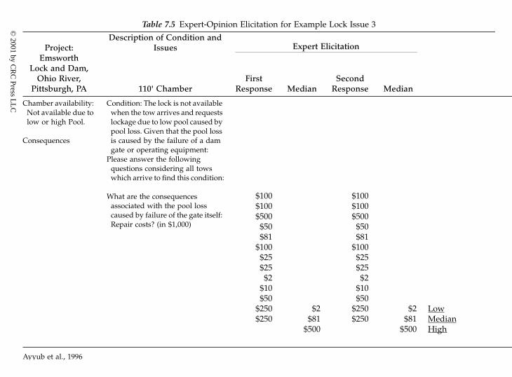
Table 7.5 Expert-Opinion Elicitation for Example Lock Issue 3
Project:Description of Condition and
Issues Expert ElicitationEmsworth
Lock and Dam,Ohio River,
Pittsburgh, PA 110' ChamberFirst
Response MedianSecond
Response Median
Chamber availability: Not available due to low or high Pool.
Consequences
Condition: The lock is not available when the tow arrives and requests lockage due to low pool caused by pool loss. Given that the pool loss is caused by the failure of a dam gate or operating equipment:
Please answer the following questions considering all tows which arrive to find this condition:
What are the consequences associated with the pool loss caused by failure of the gate itself: Repair costs? (in $1,000)
$100$100$500$50$81
$100$25$25$2
$10$50
$250$250
$2$81
$500
$100$100$500$50$81
$100$25$25$2
$10$50
$250$250
$2$81
$500
LowMedianHigh
Ayyub et al., 1996
© 2001 by C
RC
Press LL
C
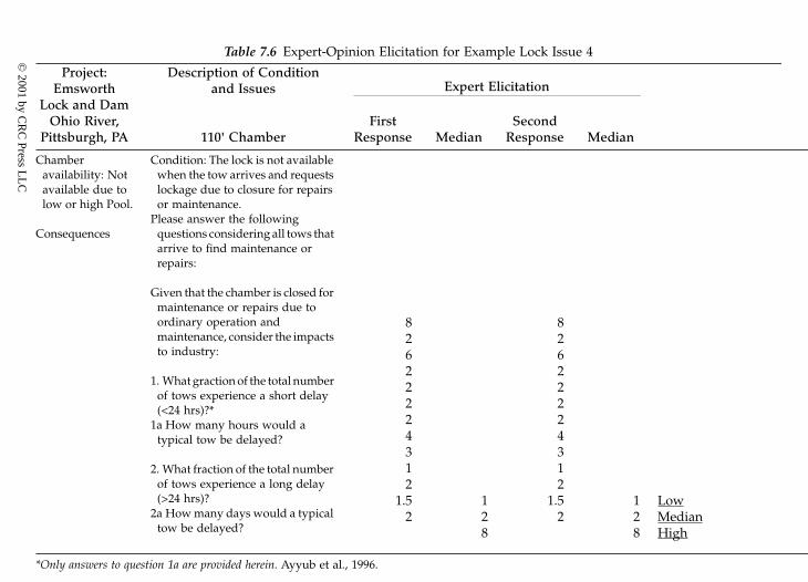
Table 7.6 Expert-Opinion Elicitation for Example Lock Issue 4
Project:Emsworth
Lock and Dam Ohio River,
Pittsburgh, PA
Description of Conditionand Issues Expert Elicitation
110' ChamberFirst
Response MedianSecond
Response Median
Chamberavailability: Not available due to low or high Pool.
Consequences
Condition: The lock is not available when the tow arrives and requests lockage due to closure for repairs or maintenance.
Please answer the following questions considering all tows that arrive to find maintenance or repairs:
Given that the chamber is closed for maintenance or repairs due to ordinary operation and maintenance, consider the impacts to industry:
1. What graction of the total number of tows experience a short delay (<24 hrs)?*
1a How many hours would a typical tow be delayed?
2. What fraction of the total number of tows experience a long delay (>24 hrs)?
2a How many days would a typical tow be delayed?
82622224312
1.52
128
82622224312
1.52
128
LowMedianHigh
*Only answers to question 1a are provided herein. Ayyub et al., 1996.
© 2001 by C
RC
Press LL
C

7.3 Economic consequences of floods7.3.1 Background
Ayyub and Moser (2000) documented the use of methods and results ofusing expert-opinion elicitation for developing structural and content depth-damage relationships for single-family one-story homes without basements,residential content-to-structure value ratios (CSVR), and vehicle depth-dam-age relationships in the Feather River Basin of California. These damagefunctions consider exterior building material such as brick, brick veneer,wood frame, and metal siding. The resulting consequences can be used inrisk studies and in making risk-based decisions.
The expert-opinion elicitation was performed during a face-to-face meet-ing of members of an expert panel developed specifically for the issues underconsideration. The meeting of the expert panel was conducted after provid-ing the experts, in advance of the meeting, background information, objec-tives, list of issues, and anticipated outcomes from the meeting. In Ayyuband Moser (2000), additional details on the different components of theexpert elicitation process are described, the process itself is outlined anddiscussed, and the results are documented.
7.3.2 The Feather River Basin
7.3.2.1 Levee failure and consequent floodingIn January 1997, the eastern levee of the Feather River failed, causing majorflooding near the Yuba County town of Arboga. Floodwaters inundatedapproximately 12,000 acres and damaged over 700 structures. Although thearea was primarily agricultural, approximately 600 residential structureswere affected by flooding. This area had a wide range of flooding depths,from maximum depths about 20 feet (structures totally covered) in the southnear the levee break to minimal depths. Residential damage from the flood-ing was documented as a joint project of the Corps of Engineers FloodDamage Data Collection and the Sacramento-San Joaquin River Basin Com-prehensive Study. The population of homes within the flood plain of theJanuary 1997 flood defines the study area in this investigation.
7.3.2.2 Flood characteristicsThe January 1997 flooding resulted from a trio of subtropical storms. Overa 3-day period, warm moist winds from the southwest, blowing over theSierra Nevada, poured more than 30 inches of rain onto watersheds that werealready saturated by one of the wettest Decembers on record. The first of thestorms hit Northern California on December 29, 1996, with less than expectedprecipitation totals. Only 0.24 inch of rainfall was reported in Sacramento.On December 30, 1996, the second storm arrived. The third and most severestorm hit late December 31, 1996, and lasted through January 2, 1997.
© 2001 by CRC Press LLC

Precipitation totals at lower elevations in the central valley were notunusually high, in contrast to extreme rainfall in the upper watersheds.Downtown Sacramento, for example, received 3.7 in of rain from December26, 1996, through January 2, 1997. However, Blue Canyon (elevation 5000 ft)in the American River Basin received over 30 in of rainfall, thus providingfor an orographic ratio of 8 to 1. A typical storm for this region would yieldan orographic ratio of between 3 or 4 between these two locations.
In addition to the trio of subtropical storms, snowmelt also contributedto the already large runoff volumes. Several days before Christmas 1996, acold storm from the Gulf of Alaska brought snow to low elevations in theSierra Nevada foothills. Blue Canyon, for example, had a snowpack with 5in of water content. The snowpack at Blue Canyon, as well as the snowpackat lower elevations, melted when the trio of warmer storms hit. Not muchsnowpack loss was observed, however, at snow sensors over 6000 ft inelevation in the northern Sierra. The effect of the snowmelt was estimatedto contribute approximately 15 percent to runoff totals.
Prior to the late December storms, rainfall was already well above nor-mal in the Sacramento River Basin. In the northern Sierra, total Decemberprecipitation exceeded 28 in, the second wettest December on record,exceeded only by the 30.8 in in December 1955.
On the Yuba River, available storage in New Bullards Reservoir was over200 percent of flood management reservation space on December 1, 1996.By the end of the storm, available space was about 1 percent of flood pool.Oroville Reservoir, on the Feather River, began December with just over100% flood management reservation space. At the completion of the stormsin early January, approximately 27% space remained available.
The hydrologic conditions of the January, 1997 flooding of the FeatherRiver Basin were used as the basis for developing depth-damage relation-ships and CSVR. These hydrologic conditions resulted in high-velocity flood-ing from an intense rainfall and a levee failure. A scenario that gives furtherdetails on flood characteristics was defined and used in the study.
7.3.2.3 Building characteristicsMost of the residential properties affected by the January 1997 flood weresingle-story, single-family structures with no basements. The primary con-struction materials were wood or stucco. Few properties in the study areawere two-story, and nearly none had basements. It may be useful to differ-entiate one-story on slab from one-story on raised foundations.
The study is limited to the following residential structural types withoutbasement:
One-story on slab, One-story on piers and beams (i.e., raised foundations), andMobile homes.
© 2001 by CRC Press LLC
7.3.2.4 Vehicle characteristicsVehicle classes included in the study were
Sedan cars,Pickup trucks, sport utility vehicles, vans, andMotorcycles.
7.3.3 Example issues and results
7.3.3.1 Structural depth-damage relationships Background: The hydrologic conditions of the January 1997 flooding of theFeather River Basin were used as the basis for developing these values. Thesehydrologic conditions resulted in high-velocity flooding from an intenserainfall and a levee failure.
Issues: What are the best estimates of the median percent damage values asa function of flood depth to a residential structure for all types? Also, whatis the confidence level in the opinion of the expert (low, medium, or high)?
The study is limited to the following residential structural types:
• Type 1 — one-story without basement on slab• Type 2 — one-story on piers and beams (i.e., raised foundation)• Type 3 — mobile homes
The experts discussed the issues that produced the assumptions providedin Table 7.7. In this study, structural depth-damage relationships were devel-oped based on expert opinions as provided in sample results in Table 7.8. Eachexpert needed to provide his/her best estimate of the median value for percentdamage and respondents’ levels of confidence in their estimates. Samplerevised depth damage relationships are shown in Figures 7.2a and 7.2b.
7.3.3.2 Content depth-damage relationships Background: The hydrologic conditions of the January 1997 flooding of theFeather River Basin were used as the basis for developing these values. Thesehydrologic conditions resulted in high-velocity flooding from an intenserainfall and a levee failure.
Issues: What are the best estimates of the median percent damage values asa function of flood depth to the content of residential structures for all types?Also, what is the confidence level in the opinion of the expert (low, medium,or high)?
The study is limited to the following residential structural types:
• Types 1 and 2 — one-story without basement on slab or one-storyon piers and beams (i.e., raised foundation)
• Type 3 — mobile homes
© 2001 by CRC Press LLC

The experts discussed the issues that produced the assumptions provided inTable 7.9. In this study, content depth-damage relationships were developedbased on expert opinions as provided in the sample Table 7.10. Sample reviseddepth damage relationships are shown in Figures 7.3a and 7.3b.
Table 7.7 Summary of Supportive Reasoning and Assumptionsby Experts for Structure Value
House Types 1 and 2 House Type 3
Median house size of 1400 SFWood frame homesMedian house value of $90,000 with land
Median land value of $20,000Median price without land is about $50 per SF
Median house age of 8 yearsType 2 has HVAC and sewer lines below finished floor
Percentages are of depreciated replacement value of houses
Flood without flow velocitySeveral days of flood durationFlood water is not contaminated but has sediment without large debris
No septic field damagesAllow for cleanup cost
Median size of 24 ft by 60 ft (1200 SF)Wood frame homesMedian house value of $30,000 without land
Median house age of 8 yearsFinished floor is 3 ft above ground level8 ft ceiling heightHVAC and sewer lines below finishedfloor
Percentages are of depreciated replacement value of houses
Flood without flow velocitySeveral days of flood durationFlood water is not contaminated but has sediment without large debris
No septic field damagesAllow for cleanup cost
Figure 7.2a Percent damage to a residential structure Type 1: one-story withoutbasement on slab.
100.090.0
80.0
70.060.050.040.030.020.010.0
0.0-1.0 1.0 3.0 5.0 7.0 9.0 11.0
Expert 1
Expert 2
Expert 3
Expert 4
Expert 5
Expert 6
Expert 7
Dam
age
(%)
Depth (ft.)
© 2001 by CRC Press LLC

7.3.3.3 Content-to-structure value ratiosBackground: The hydrologic conditions of the January 1997 flooding of theFeather River Basin were used as the basis for developing these ratios. Thesehydrologic conditions resulted in high-velocity flooding from an intenserainfall and a levee failure.
Issues: What are the best estimates of the median values of a residentialstructure, its content, and their ratios (CSVR) for all types? Also, what is theconfidence level in the opinion of the expert (low, medium, or high)?
The study is limited to the following residential structural types:
• Types 1 and 2 — one-story without basement on slab or one-storyon piers and beams (i.e., raised foundation)
• Type 3 — mobile homes
The experts discussed the issues that produced the assumptions pro-vided in Table 7.11. In this study, the best estimates of the median value ofstructures, the median value of contents, and the ratio of content to structurevalue were developed for these types based on expert opinions as providedin sample Table 7.12. Sample CVSRs are shown in Figure 7.4.
7.3.3.4 Vehicle depth-damage relationshipsBackground: The hydrologic conditions of the January 1997 flooding of theFeather River Basin were used as the basis for developing these values. Thesehydrologic conditions resulted in high-velocity flooding from an intenserainfall and a levee failure.
Figure 7.2b Aggregated percent damage to a residential structure Type 1: one-storywithout basement on slab.
100.090.080.070.060.050.040.030.020.010.00.0
-1.0 1.0 3.0 5.0 7.0 9.0 11.0
Depth (ft.)
Dam
age
(%)
Minimum
Maximum
25%
50%
75%
© 2001 by CRC Press LLC

Table 7.8 Percent Damage to a Residential Structure Type 1: One-Story without Basement on Slab
Initial Estimate: % Damage by Expert Aggregated OpinionsDepth 1 2 3 4 5 6 7 Min 25% 50% 75% Max
-1 4 0 3 0 0 0 0 0 0 0 1.5 4-0.5 4 0 5 0 0 0 0 0 0 0 2 50 5 0 10 5 0 10 0 0 0 5 7.5 100.5 10 40 12 7 10 13 45 7 10 12 26.5 451 15 40 25 9 20 15 55 9 15 20 32.5 551.5 20 40 28 11 30 20 55 11 20 28 35 552 30 40 35 13 30 20 60 13 25 30 37.5 603 40 40 35 15 40 30 60 15 32.5 40 40 604 48 40 40 25 70 50 65 25 40 48 57.5 705 53 65 40 40 70 85 70 40 46.5 65 70 856 65 65 45 50 70 85 75 45 57.5 65 72.5 857 68 70 75 70 80 90 75 68 70 75 77.5 908 70 75 80 90 80 90 75 70 75 80 85 909 73 85 95 100 95 90 75 73 80 90 95 100
10 80 85 100 100 100 100 80 80 82.5 100 100 10011 83 85 100 100 100 100 80 80 84 100 100 10012 85 85 100 100 100 100 80 80 85 100 100 100
© 2001 by C
RC
Press LL
C

Table 7.8 cont.
Revised Estimate: % Damage by Expert Aggregated OpinionsDepth 1 2 3 4 5 6 7 Min 25% 50% 75% Max
-1 1 0 3 0 0 0 5 0 0 0 2 5-0.5 1 0 5 0 0 0 10 0 0 0 3 100 10 15 10 5 5 15 35 5 7.5 10 15 350.5 10 40 25 40 20 45 45 10 22.5 40 42.5 451 25 40 30 40 20 45 45 20 27.5 40 42.5 451.5 25 40 40 40 30 45 45 25 35 40 42.5 452 35 40 45 40 30 45 45 30 37.5 40 45 453 40 40 45 40 40 70 45 40 40 40 45 704 48 40 55 40 70 80 55 40 44 55 62.5 805 53 65 55 50 70 85 60 50 54 60 67.5 856 65 65 70 60 70 85 65 60 65 65 70 857 68 65 75 85 80 95 75 65 71.5 75 82.5 958 70 65 80 85 85 95 75 65 72.5 80 85 959 73 85 95 85 85 95 75 73 80 85 90 95
10 80 85 100 85 85 95 80 80 82.5 85 90 10011 83 85 100 85 85 95 80 80 84 85 90 10012 85 85 100 85 85 95 80 80 85 85 90 100
Confidence High High High High High High High
© 2001 by C
RC
Press LL
C

Issues: What are the best estimates of the median percent damage values asa function of flood depth to vehicles for all types? Also, what is the confidencelevel in the opinion of the expert (low, medium, or high)?
The study is limited to the following residential vehicle classes asfollows:
• Type 1 — sedan cars• Type 2 — pickup trucks, sports utility vehicles, and vans• Type 3 — motorcycles
The experts discussed the issues that produced the assumptions providedin Table 7.13. In this study, the best estimates of the median value of vehicledepth-damage relationships were developed based on expert opinions asprovided in sample Table 7.14. Sample relationships are shown in Figures7.5a and 7.5b.
Table 7.9 Summary of Supportive Reasoning and Assumptionsby Experts for Content Value
House Types 1, 2 and 3
As a guide, the insurance industry uses 70% ratio for the content to structure valueMedian house value of $90,000 with landMedian land value of $20,000Garage or shed contents are includedMedian content age of 8 yearsPercentages are of depreciated replacement value of contentsFlood without flow velocitySeveral days of flood durationFlood water is not contaminated but has sediment without large debrisAllow for cleanup costInsufficient time to remove (i.e. protect) contents
© 2001 by CRC Press LLC

Table 7.10 Percent Damage to Contents of Residential StructureTypes 1 and 2: One-Story on Slab or on Piers and Beams
Initial Estimate: % Damage by Expert Aggregated OpinionsDepth 1 2 3 4 5 6 7 Min 25% 50% 75% Max
-1 0.5 0 3 0 0 10 0 0 0 0 1.8 10-0.5 0.5 0 5 0 0 20 0 0 0 0 2.8 200 2 30 15 0 0 40 5 0 1 5 22.5 400.5 2 40 35 20 50 40 10 2 15 35 40 501 15 50 35 40 50 40 20 15 27.5 40 45 501.5 27 60 40 50 60 40 20 20 33.5 40 55 602 35 70 40 60 70 60 40 35 40 60 65 703 47 80 70 70 80 80 40 40 58.5 70 80 804 55 80 70 80 80 90 60 55 65 80 80 905 80 80 70 90 90 90 60 60 75 80 90 906 90 80 70 100 100 90 85 70 82.5 90 95 1007 90 80 75 100 100 95 95 75 85 95 97.5 1008 90 85 85 100 100 100 100 85 87.5 100 100 1009 90 85 90 100 100 100 100 85 90 100 100 100
10 90 85 90 100 100 100 100 85 90 100 100 10011 90 85 90 100 100 100 100 85 90 100 100 10012 90 90 90 100 100 100 100 90 90 100 100 100
© 2001 by C
RC
Press LL
C
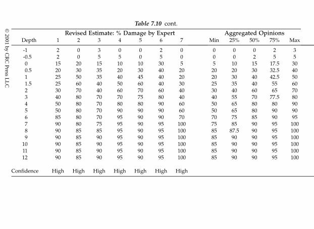
Table 7.10 cont.
Revised Estimate: % Damage by Expert Aggregated OpinionsDepth 1 2 3 4 5 6 7 Min 25% 50% 75% Max
-1 2 0 3 0 0 2 0 0 0 0 2 3-0.5 2 0 5 5 0 5 0 0 0 2 5 50 15 20 15 10 10 30 5 5 10 15 17.5 300.5 20 30 35 20 30 40 20 20 20 30 32.5 401 25 50 35 40 45 40 20 20 30 40 42.5 501.5 25 60 40 50 60 40 30 25 35 40 55 602 30 70 40 60 70 60 40 30 40 60 65 703 40 80 70 70 75 80 40 40 55 70 77.5 804 50 80 70 80 80 90 60 50 65 80 80 905 50 80 70 90 90 90 60 50 65 80 90 906 85 80 70 95 90 90 70 70 75 85 90 957 90 80 75 95 90 95 100 75 85 90 95 1008 90 85 85 95 90 95 100 85 87.5 90 95 1009 90 85 90 95 90 95 100 85 90 90 95 100
10 90 85 90 95 90 95 100 85 90 90 95 10011 90 85 90 95 90 95 100 85 90 90 95 10012 90 85 90 95 90 95 100 85 90 90 95 100
Confidence High High High High High High High
© 2001 by C
RC
Press LL
C
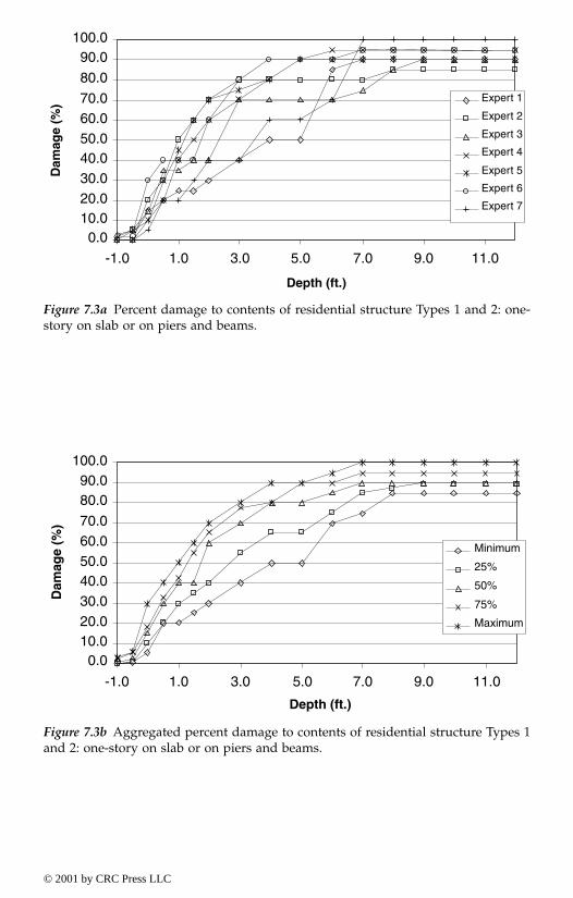
Figure 7.3a Percent damage to contents of residential structure Types 1 and 2: one-story on slab or on piers and beams.
Figure 7.3b Aggregated percent damage to contents of residential structure Types 1and 2: one-story on slab or on piers and beams.
100.090.0
80.0
70.060.050.040.030.020.010.0
0.0
-1.0 1.0 3.0 5.0 7.0 9.0 11.0
Expert 1
Expert 2
Expert 3
Expert 4
Expert 5
Expert 6
Expert 7
Dam
age
(%)
Depth (ft.)
100.090.080.0
70.060.050.040.030.020.010.0
0.0
-1.0 1.0 3.0 5.0 7.0 9.0 11.0
Dam
age
(%)
Depth (ft.)
Minimum
Maximum
25%
50%
75%
© 2001 by CRC Press LLC

Table 7.11 Summary of Supportive Reasoning and Assumptions by Experts for Content to Structure Value Ratio (CSVR)
House Types 1, 2 and 3
As a guide, the insurance industry uses 70% ratio for the content to structure value
Median house value of $90,000 with landMedian land value of $20,000Garage or shed contents are includedMedian content age of 8 yearsUse depreciated replacement value of structure and contentsInsufficient time to remove (i.e. protect) contents
Figure 7.4 Content to structure value ratios (CSVR) for Types 1 and 2: one-story onslab or on piers and beams.
Low
Best
High
1.000.900.800.700.600.500.400.300.200.100.00
1 2 3 4 5 6 7
Min
25%
50%
75%
Max
Co
nte
nt
to S
tru
ctu
re P
rice
Rat
io
Expert
© 2001 by CRC Press LLC
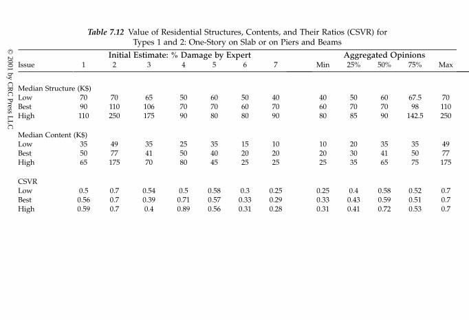
Table 7.12 Value of Residential Structures, Contents, and Their Ratios (CSVR) forTypes 1 and 2: One-Story on Slab or on Piers and Beams
Initial Estimate: % Damage by Expert Aggregated OpinionsIssue 1 2 3 4 5 6 7 Min 25% 50% 75% Max
Median Structure (K$)Low 70 70 65 50 60 50 40 40 50 60 67.5 70Best 90 110 106 70 70 60 70 60 70 70 98 110High 110 250 175 90 80 80 90 80 85 90 142.5 250
Median Content (K$)Low 35 49 35 25 35 15 10 10 20 35 35 49Best 50 77 41 50 40 20 20 20 30 41 50 77High 65 175 70 80 45 25 25 25 35 65 75 175
CSVRLow 0.5 0.7 0.54 0.5 0.58 0.3 0.25 0.25 0.4 0.58 0.52 0.7Best 0.56 0.7 0.39 0.71 0.57 0.33 0.29 0.33 0.43 0.59 0.51 0.7High 0.59 0.7 0.4 0.89 0.56 0.31 0.28 0.31 0.41 0.72 0.53 0.7
© 2001 by C
RC
Press LL
C

Table 7.12 cont.
Revised Estimate: % Damage by Expert Aggregated OpinionsIssue 1 2 3 4 5 6 7 Min 25% 50% 75% Max
Median Structure (K$)Low 70 70 77 50 60 50 50 50 50 60 70 77Best 90 80 82 70 70 60 70 60 70 70 81 90High 110 90 94 90 80 75 90 75 85 90 92 110
Median Content (K$)Low 35 49 40 25 35 15 10 10 20 35 37.5 49Best 50 50 42 50 40 20 20 20 30 42 50 50High 65 51 50 80 45 25 30 25 37.5 50 58 80
CSVRLow 0.5 0.7 0.52 0.5 0.58 0.3 0.2 0.2 0.4 0.5 0.55 0.7Best 0.56 0.63 0.51 0.71 0.57 0.33 0.29 0.29 0.42 0.56 0.6 0.71High 0.59 0.57 0.53 0.89 0.56 0.33 0.33 0.33 0.43 0.56 0.58 0.89
Confidence High High Medium High High High High
© 2001 by C
RC
Press LL
C

Table 7.13 Summary of Supportive Reasoning and Assumptions by Experts for Vehicle Damage
Vehicle Types 1 and 2
Median vehicle age of 5 yearsPercentages are of depreciated replacement value of vehiclesFlood without flow velocitySeveral days of flood durationFlood water is not contaminated but has sediment without large debris
Allow for cleanup cost
Figure 7.5a Percent damage to a vehicle Type 1: sedan cars.
Figure 7.5b Aggregated percent damage to a vehicle Type 1: sedan cars.
100.090.0
80.0
70.060.050.040.030.020.010.0
0.0
0.0 1.0 2.0 3.0 4.0 5.0
Expert 1
Expert 2
Expert 3
Expert 4
Expert 5
Expert 6
Expert 7
Dam
age
(%)
Depth (ft.)
100.090.0
80.0
70.060.050.040.030.020.010.00.0
0.0 1.0 2.0 3.0 4.0 5.0 6.0
Dam
age
(%)
Depth (ft.)
Minimum
Maximum
25%
50%
75%
© 2001 by CRC Press LLC

Table 7.14 Percent Damage to a Vehicle Type 1: Sedan Cars
Initial Estimate: % Damage by Expert Aggregated OpinionsDepth 1 2 3 4 5 6 7 Min 25% 50% 75% Max
0 0 0 0 0 0 0 0 0 0 0 0 00.5 5 0 5 0 0 0 0 0 0 0 2.5 51 20 0 30 10 25 5 10 0 7.5 10 22.5 301.5 25 0 50 15 25 15 50 0 15 25 37.5 502 35 30 80 20 30 20 60 20 25 30 47.5 802.5 50 35 100 40 70 40 70 35 40 50 70 1003 60 40 100 50 70 60 90 40 55 60 80 1004 100 40 100 100 80 80 100 40 80 100 100 1005 100 50 100 100 95 80 100 50 87.5 100 100 100
Revised Estimate: % Damage by Expert Aggregated OpinionsDepth 1 2 3 4 5 6 7 Min 25% 50% 75% Max
0 0 0 0 0 0 0 0 0 0 0 0 00.5 10 0 5 0 0 2 0 0 0 0 3.5 101 25 10 20 20 20 10 20 10 15 20 20 251.5 35 30 50 25 25 40 30 25 27.5 30 37.5 502 40 40 80 30 30 50 50 30 35 40 50 802.5 50 50 100 40 60 60 70 40 50 60 65 1003 60 100 100 50 70 80 80 50 65 80 90 1004 100 100 100 100 100 80 100 80 100 100 100 1005 100 100 100 100 100 80 100 80 100 100 100 100
Confidence High High High High High Medium High
© 2001 by C
RC
Press LL
C

Bibliography
Abraham, D.M., Bernold, L.E., and Livingston, E.E., 1989. Emulation for controlsystem analysis in automated construction. J. Comput. Civ. Eng., 3(4), 320–332.
Alpert, M. and Raiffa, H., 1982, A progress report on the training of probabilityassessors, in Kahneman et al., (Eds.), Judgement Under Uncertainty, Heuristicsand Biases, Cambridge University Press, Cambridge, 294–306.
Alvi, I.A. and Ayyub, B.M., 1990, Analysis of system performance under stochasticand fuzzy uncertainty, NAFIPS.
Amendola, A., 1986. System Reliability Benchmark Exercise, I and II, EUR-10696, EN/I,Joint Research Center of Ispra, Italy.
American Institute of Aeronautics and Astronautics, 1998. Guide for Verification andValidation of Computational Fluid Dynamics Simulation, AIAA G-077-1998.
American Psychological Association, 1985. Standards for Educational and Psycho-logical Testing, Washington, D.C.
ASME (American Society of Mechanical Engineers), 1993. The use of decision-analyticreliability methods in codes and standards work. CRTD 23, New York.
Ammermn, R.R. Ed. 1970. Belief, Knowledge and Truth, Charles Scribners Sons, NewYork.
Ang, A. and Tang, W., 1975. Probability Concepts in Engineering Planning and Design,Vol. 1, John Wiley, New York.
Armstrong, D., 1973. Belief Truth and Knowledge, Cambridge University Press, Cam-bridge.
Austin, D.F. (Ed.), 1998. Philosophical Analysis: A Defense by Example, (PhilosophicalStudies Series, Vol. 39), D. Reidel Publishing Co.
Ayyub, B.M., 1994. The nature of uncertainty in structural engineering, in UncertaintyModelling and Analysis: Theory and Applications, Ayyub and Gupta (Eds.),North-Holland-Elsevier Scientific Publishers, 195–210.
Ayyub, B.M., 1991. Systems framework for fuzzy sets in civil engineering, Int. J. FuzzySets and Syst, 40(3), 491–508.
Ayyub, B.M., 1992. Generalized treatment of uncertainties in structural engineering.Analysis and Management of Uncertainty: Theory and Applications, Ayyub andGupta, (Eds.) Elsevier Science Publisher, New York, 235–246.
Ayyub, B.M., 1992. Fault Tree Analysis of Cargo Elevators Onboard Ships, BMAEngineering Report, prepared for Naval Sea System Command, U.S. Navy,Crystal City, VA.
© 2001 by CRC Press LLC

Ayyub, B.M., 1993. Handbook for Risk-Based Plant Integrity, BMA Engineering Re-port, prepared for Chevron Research and Technology Corporation, Rich-mond, CA.
Ayyub, B.M. and Chao, R.-J., 1998. Uncertainty modeling in civil engineering withstructural and reliability applications, in Uncertainty Modeling and Analysis inCivil Engineering, B. Ayyub (Ed.), CRC Press, 1–32, Chap. 1.
Ayyub, B.M. and Gupta, M.M., (Eds.), 1997. Uncertainty Analysis in Engineering andthe Sciences: Fuzzy Logic, Statistics, and Neural Network Approach, Kluwer Aca-demic Publisher.
Ayyub, B.M. and Hassan, M.H.M., 1992a. Control of construction activities: I. Systemsidentification, Civ. Eng. Sys., 9, 123–146.
Ayyub, B.M. and Hassan, M.H.M., 1992b. Control of construction activities: II. Con-dition assessment of attributes, Civ. Eng. Sys., 9, 147–204.
Ayyub, B.M. and Hassan, M.H.M., 1992c. Control of construction activities: III. Afuzzy-based controller, Civ. Eng. Sys., 9, 275–297.
Ayyub, B.M. and Lai, K.-L., 1992. Structural reliability assessment with ambiguityand vagueness in failure, Nav. Eng. J., 104(3), 21–35.
Ayyub, B.M. and McCuen, R., 1996. Numerical Methods for Engineers, Prentice Hall,Upper Saddle River, NJ.
Ayyub, B.M. and McCuen, R., 1997. Probability, Statistics and Reliability for Engineers,CRC Press, Boca Raton, FL, 1997.
Ayyub, B.M. and Moser, D.A., 2000. Economic Consequence Assessment of Floodsin the Feather River Basin of California Using Expert-Opinion Elicitation,Technical Report, Institute for Water Resources, USACE.
Ayyub, B.M., Gupta, M.M., and Kanal, L.N., 1992, Analysis and Management of Uncer-tainty: Theory and Applications, Elsevier Science Publishing Company, Inc.,New York.
Ayyub, B.M., Riley, B.C., and Hoge, M.T., 1996. Expert Elicitation of Unsatisfactory-Performance Probabilities and Consequences for Civil Works Facilities, Tech-nical Report, USACE, Pittsburgh District, PA.
Ayyub, B.M. and Haldar, A., 1984, Practical structural reliability techniques, J. Struct.Eng., 110(8), 1707–1724.
Ayyub, B.M., (Ed.), 1998, Uncertainty Modeling and Analysis in Civil Engineering, CRCPress, Boca Raton, FL.
Ayyub, B.M., Guran, A., and Haldar, A., (Eds.), 1997. Uncertainty Modeling in Vibration,Control, and Fuzzy Analysis of Structural Systems, World Scientific.
Bailey, K.D., 1994. Methods of Social Research, The Free Press, Maxwell Macmillan,New York.
Beacher, G., Expert Elicitation in Geotechnical Risk Assessment, 1999. USACE DraftReport, University of Maryland, College Park, MD.
Beck, L.J., 1965. The Metaphysics of Descartes, Oxford University Press, Oxford, UK.Bell, T.E. and Esch, K., 1989. The space shuttle: A case of subjective engineering, IEEE
Spectrum, 42–46.Bennett, J., 1990. Why is belief involuntary, Analysis, 50(2).Blair, A.N. and Ayyub, B.M., 1999. Fuzzy stochastic cost and schedule risk analysis:
MOB case study, Proc. Symp. Very Large Floating Structures, Elsevier, NorthHolland.
Blanchard, B.S., 1998. System Engineering Management, 2nd ed., John Wiley and Sons,Inc., New York.
© 2001 by CRC Press LLC

Blockley, D.I., 1975, Predicting the likelihood of structural accidents, Proc. Inst. Civ.Eng., 59, Part 2, 659–668.
Blockley, D.I., 1979a, The calculations of uncertainty in civil engineering, Proc. Inst.Civ. Eng., 67, Part 2, 313–326.
Blockley, D.I., 1979b, The role of fuzzy sets in civil engineering, Fuzzy Sets and Syst.,2, 267–278.
Blockley, D.I., 1980, The Nature of Structural Design and Safety, Ellis Horwood,Chichester, UK.
Blockley, D.I., Pilsworth, B.W., and Baldwin, J.F., 1983, Measures of Uncertainty, Civ.Eng. Syst., 1, 3–9.
Boltzmann, L., 1894, Zur Integration der Diffusionsgleichung bei variablen Diffusion-skoeffizienten, Ann. Physik, 53, Leipzig, Germany.
Bouissac, P., 1992. The construction of ignorance and the evolution of knowledge,University of Toronto Quarterly, 61(4), Summer.
Bowles, D., 1990. Risk assessment in dam safety decisionmaking. Risk-Based DecisionMaking in Water Resources, Proc. 4th Conf., Y. Y. Haimes and E.Z. Stakhiv(Eds.), 254–83.
Bradie, M., 1986. Assessing evolutionary epistemology, Biol. and Philos., 1, 401–450.Bremermann, H.J., 1962. Optimization through evolution and recombination, in Yo-
vits, M.C., Jacobi, G.T., and Goldstein, G.D. (Eds.), Self-Organizing Systems,Spartan Books, Washington, 93–106.
Brown, C.B. and Yao, J.T.P., 1983, Fuzzy sets and structural engineering, J. Struct.Eng., 109(5), 1211–1225.
Brown, C.B., 1979, A fuzzy safety measure, J. Eng. Mech. Div., 105(EM5), 855–872.Brown, C.B., 1980, The merging of fuzzy and crisp information, J. Eng. Mech. Div.,
106(EM1), 123–133.Brune, R., Weinstein, M., and Fitzwater, M., 1983. Peer Review Study of the Draft
Handbook for Human Reliability Analysis with Emphasis on Nuclear PowerPlant Applications, NUREG/CR-1278.
Campbell, D.T., 1974. Evolutionary epistemology, in P.A. Schilpp (Ed.), The Philosophyof Karl Popper, Open Court Publishing, LaSalle, IL, 1,413–463.
Chestnut, H., 1965. Systems Engineering Tools, John Wiley & Sons, Inc., New York.Chomsky, N., 1968. Language and Mind, Harcourt Brace Jovanovich, New York.Clemen, R.T., 1989. Combining forecasts: a review and annotated bibliography, Int.
J. Forecasting, 5, 559–583.Colglazier, E.W. and Weatherwax, R.K., 1986. Failure estimates for the space shuttle,
Abstracts from the Society of Risk Analysis, annual meeting, Boston, MA,Nov. 9–12, 1986, 80.
Committee on Safety Criteria for Dams, 1985. Safety of Dams: Flood and EarthquakeCriteria, National Academy Press, Washington, D.C.
Committee on the Safety of Existing Dams, 1983. Safety of Existing Dams, Evaluationand Improvement, National Research Council, National Academy Press,Washington, D.C.
Cooke, R.M., 1986. Problems with empirical bayes, Risk Analysis, 6(3), 269–272.Cooke, R.M., 1991. Experts in Uncertainty, Oxford University Press, New York.Dancy, J., 1985. Contemporary Epistemology, Basil Blackwell, Oxford, UK.De Cooman, G., 1997, Possibility theory. Int. J. G. Sys., 25(4), 291–371.De Finetti, B., 1937, English Translation in 1964 by H. Kyburg and H. Smokler (Eds.).
Studies in Subjective Probabilities, Wiley, New York.
© 2001 by CRC Press LLC
Defense Acquisition University, 1998. Risk Management Guide, Defense SystemsManagement College Press, Fort Belvoir, VA.
DeKay, M.L. and McClelland, G.H., 1993, Predicting loss of life in cases of dam failureand flash flood, Risk Analysis, 13(2), 193–205.
Dempster, A.P., 1976a. Upper and lower probabilities induced by multivalued map-ping, Ann. Math. Stat., 38(2), 325–339.
Dempster, A.P., 1976b. Upper and lower probabilities inferences based on a samplefrom a finite univariate population, Biometrika, 54(3–4), 515–528.
Dewey, J., 1929. The Quest For Certainty, Minton, Balch and Co., New York.di Carlo, C.W., 1998. Evolutionary Epistemology and the Concept of Ignorance, PhD
Thesis, University of Waterloo, Ontario, Canada.Dombi, J., 1982. A general class of fuzzy operators, the De Morgan class of fuzzy
operators and fuzziness measures induced in fuzzy operators, Fuzzy Sets andSystems, 8, 149–163.
Dong, W-M. and Wong, F.S., 1986a, From uncertainty to approximate reasoning: Part1: Conceptual models and engineering interpretations, Civ. Eng. Sys., 3(3),143–154.
Dong, W-M. and Wong, F.S., 1986b, From uncertainty to approximate reasoning: Part2: Reasoning with algorithmic rules, Civ. Eng. Sys., 3(4), 192–202.
Dong, W-M. and Wong, F.S., 1986c, From uncertainty to approximate reasoning: Part3: Reasoning with conditional rules, Civ. Eng. Sys., 3(5), 112–121.
Dretske, F., 198l. Knowledge and the Flow of Information, MIT Press, Cambridge, MA.Driver, J., 1989. The virtues of ignorance, J. Philos., 86.Dubois, D. and Prade, H., 1988. Possibility Theory. Plenum Press, New York.Dubois, D. and Prade, H., 1980. On several representation of an uncertain body of
evidence, in Fuzzy Information and Decision Processes, Gupta, and Sanchez(Eds.), North-Holland, New York, 167–181.
Duncan, R. and Weston-Smith, M., Eds. 1977. The Encyclopedia of Ignorance, PergamonPress Ltd., New York.
Durant, W., 1991. Story of Philosophy: The Lives and Opinions of the World’s GreatestPhilosophers, Pocket Books.
Eldukair, Z.A. and Ayyub, B.M., 1991. Analysis of recent U.S. structural and construc-tion failures, J. Performance of Constructed Facilities, 5(1), 57–73.
Ferrell, W.R., 1985. Combining individuals judgments, in Wright, G. (Ed.), BehavioralDecision Making, Plenum, NY.
Ferrell, W.R., 1994. Discrete subjective probabilities and decision analysis: elicitation,calibration and combination, in Wright, G., and Ayton, P. (Eds.), SubjectiveProbability, John Wiley and Sons, New York.
Ferson, S., Root, W., and Kuhn, R., 1999. RAMAS Risk Calc: Risk Assessment withUncertain Numbers, Applied Biomathematics, Inc., Setauket, NY.
Fisher, R.A., 1930. The Genetical Theory of Natural Selection, Oxford University Press,Oxford, UK.
Frank, M.J., 1979. On the simultaneous associativity of F(x,y) and x+y–F(x,y), Aequa-tiones Mathematicae, 19(2–3), 194–226.
Frank, M.J., Nelson, R.B., and Schweizer, B., 1987, Best-possible bounds for the dis-tribution of a sum — a problem of Kolmogorov, Probability Theory and RelatedFields, 74, 199–211.
Freeman, W.M., 1969. Readings from Scientific America: Science, Conflict and Society, SanFrancisco.
© 2001 by CRC Press LLC

French, S., 1985. Group consensus probability distributions: a critical survey, J.M.Bernardo et al. (Eds.), Bayesian Statistics, Elsevier, North Holland, 183–201.
Furuta, H., Fu, K.S., and Yao, J.T.P., 1985, Structural engineering applications of expertsystems, Computer Aided Design, 17(9), 410–419.
Furuta, H., Shiraishi, N., and Yao, J.T.P., 1986, An expert system for evaluation ofstructural durability, Proc. 5th OMAE Symp., 1, 11–15.
Galanter, E., 1962. The direct measurement of utility and subjective probability, Am.J. Psych., 75, 208–220.
Garey, M.R. and Johnson, D.S., 1979. Computers and Intractability: A Guide to the Theoryof NP-Completeness, W.H. Freeman, San Francisco.
Genest, C. and Zidek, J., 1986. Combining probability distributions: critique and anannotated bibliography, Stat. Sci., 1(1), 114–148.
Goldman, A., 1993. Philosophical Applications of Cognitive Science, Westview Press,Boulder, CO.
Gustafson, D.H., Shukla, R.K., Delbecq, A., and Walster, G.W., 1973. A comparativestudy of differences in subjective likelihood estimates made by individuals,interacting groups, delphi groups, and nominal groups, Organizational Behav-ior and Human Performance 9, 200–291.
Hackett, C., 1969. The origin of speech, Scientific American 203, 88–111.Haldar, A., Guran, A., and Ayyub, B.M., (Eds.), 1997. Uncertainty Modeling in Finite
Element, Fatigue, and Stability of Systems, World Scientific.Hall, A.D., 1962. A Method for Systems Engineering. D. Van Nostrand Company, Inc.,
Princeton, NJ.Hall, A.D., 1989. Metasystems Methodology, A New Synthesis and Unification. Pergamon
Press, New York, NY.Hall, J.W., Blockley, D.I., and Davis, J.P., 1998, Uncertain inference using interval
probability theory, Int. J. Approximate Reasoning, 19(3,4), 247–264.Hallden, S., 1986. The Strategy of Ignorance: From Decision Logic to Evolutionary Episte-
mology, Library of Theoria, Stockholm.Harr, M.E., 1987. Reliability-Based Design in Civil Engineering, McGraw-Hill Book
Company, New York.Hartford, D.N.D., 1995, How Safe is Your Dam? Is it Safe Enough?, B.C. Hydro, Main-
tenance, Engineering, and Projects, Burnaby, BC.Hartley, R.V., L., 1928, Transmission of information, The Bell Systems Technical J., 7(3),
535–563.Hassan, M.H.M. and Ayyub, B.M., 1994. Multi-attribute fuzzy control of construction
activities, in Uncertainty Modelling and Analysis: Theory and Applications, Ayyuband Gupta, (Eds.), North-Holland-Elsevier Scientific Publishers, 271–286.
Hassan, M.H.M., Ayyub, B.M., and Bernold, L., 1992. Fuzzy–based real-time controlof construction activities, Analysis and Management of Uncertainty: Theory andApplications, Ayyub, Gupta, and Kanal (Eds.), North-Holland-Elsevier Scien-tific Publishers, 331–350.
Hassan, M.H.M. and Ayyub, B.M., 1993a. Multi-attribute control of constructionactivities, Civ. Eng. Sys., 10, 37–53.
Hassan, M.H.M. and Ayyub, B.M., 1993b. A fuzzy controller for construction activi-ties, Fuzzy Sets and Systems, North-Holland, 56(3), 253–271.
Hassan, M.H.M. and Ayyub, B.M., 1997. Structural fuzzy control, in UncertaintyModeling in Vibration, Control and Fuzzy Analysis of Structural Systems, Ayyub,Guran, and Haldar (Eds.), World Scientific, 179–232, Chap. 7.
© 2001 by CRC Press LLC

Helmer, O., 1968. Analysis of the future: the delphi method, and the delphi method— an illustration, in J. Bright (Ed.), Technological Forecasting for Industry andGovernment, Prentice Hall, Englewood Cliffs, NJ.
Henley, E.J. and Kumamoto, H., 1981. Reliability Engineering and Risk Assessment,Prentice-Hall, Inc., Englewood Cliffs, NJ., 1981.
Higashi, M. and Klir, G.J., 1983, Measures of uncertainty and information based onpossibility distributions, Int. J. Gen. Sys., 8(3), 43–58.
Honderich, H. (Ed.), 1995. The Oxford Companion to Philosophy, Oxford UniversityPress, New York.
Horgan, John, 1996. The End of Science. Addison-Wesley Publishing Co., Reading, MA.Horgan, Terry (Ed.), 1995. Vagueness. The Spindel Conference 1994. Southern J.
Philos., 33 (Supplement).Horwich, P., 1987. Asymmetries in Time: Problems in the Philosophy of Science, MIT Press,
Cambridge, MA.Ishizuka, M., Fu, K.S., and Yao, J.T.P., 1981, A rule-inference method for damage
assessment, Preprint 81–502, St. Louis, MO.Ishizuka, M., Fu, K.S., and Yao, J.T.P., 1983, Rule-based damage assessment system
for existing structures, Solid Mech. Arch., 8, 99–118.Itoh, S. and Itagaki, H., 1989, Application of fuzzy-Bayesian analysis to structural
reliability, Proceedings 5th Int. Conf. Struct. Safety and Reliability, 3, A. H-S. Ang,M. Shinozuka, and G.I. Schuëller (Eds.), 1771–1774.
Johnson, O.A., 1979. Ignorance and irrationality: a study in contemporary scepticism,Philos. Res. Arch., 5,(13) 10.
Johnson-Laird, P., 1988. The Computer and the Mind: An Introduction to Cognitive Science.Harvard University Press, Cambridge, MA.
Kahn, H., 1960. On Thermonuclear War, Free Press, New York.Kahn, H. and Wiener, A.J., 1967. The Year 2000: A Framework for Speculation, Macmillan,
New York.Kahneman, D., Slovic, P., and Tversky, A. (Eds.), 1982. Judgment Under Uncertainty:
Heuristics and Biases. Cambridge University Press, Cambridge.Kaneyoshi, M., Tanaka, H., Kamei, M., and Furuta, H., 1990, Optimum cable tension
adjustment using fuzzy regression analysis, 3rd WG 7.5 Working Conferenceon Reliability and Optimization of Structural Systems, International Federation forInformation Processing, University of California, Berkeley, CA.
Kaufman, A. and Gupta, M.M., 1985. Introduction to Fuzzy Arithmetic, Theory andApplications, Van Nostrand Reinhold Co., New York, 1985.
Kaufmann, A., 1975. Introduction to the Theory of Fuzzy Subsets, Academic Press, NewYork, (Translated by D. L. Swanson).
Klir, G.J., 1969. An Approach to General Systems Theory. Van Nostrand Reinhold Com-pany, New York.
Klir, G.J., 1999, On fuzzy-set interpretation of possibility theory, Fuzzy Sets and Sys.,108(3), 263–273.
Klir, G.J., 1985, Architecture of Systems Problem Solving, Plenum Press, New York.Klir, G.J. and Cooper, J.A., 1996. On constraint fuzzy arithmetic, Proceedings 5th IEEE
Int. Conf. Sys., 1693–1699.Klir, G.J. and Folger, T.A., 1988. Fuzzy Sets, Uncertainty, and Information, Prentice Hall,
New Jersey.Klir, G.J. and Wierman, M.J., 1999. Uncertainty-based information: elements of gen-
eralized information theory. Studies in Fuzziness and Soft Computing, Physica-Verlag, New York.
© 2001 by CRC Press LLC

Klir, G.J. and Yuan, B., 1995. Fuzzy Sets, Fuzzy Logic, and Fuzzy Sets: Selected Papers byLotfi Zadeh. World Scientific, Singapore, Indonesia.
Krueger, R.A. and Casey, M.A., 2000. Focus Groups: A Practical Guide for AppliedResearch. 3rd ed., Sage Publication, Thousand Oaks, CA.
Kumamoto, H. and Henley, E.J., 1996. Probabilistic Risk Assessment and Managementfor Engineers and Scientists, 2nd ed., IEEE Press, New York.
Lai, K.-L. Lai, 1992. Generalized Uncertainty in Structural Reliability Assessment,PhD Dissertation, University of Maryland, College Park, MD.
Lai, K.-L. and Ayyub, B.M., 1994. Generalized uncertainty in structural reliabilityassessment, Civ. Eng. Syst., 11(2), 81–110.
Langer, E., 1975. The illusion of control, J. of Personality Soc. Psych., 32, 311–328.Levi, I., 1977. Four types of ignorance, Soc. Res., 44, Winter.Lichtenstein, S. and Newman, J.R., 1967. Empirical scaling of common verbal phrases
associated with numerical probabilities, Psychonometric Science, 9(10), 563–564.Lindley, D., 1970. Introduction to Probability and Statistics from a Bayesian Viewpoint,
Cambridge University Press, UK.Linstone, H.A. and Turoff, M., 1975. The Delphi Method, Techniques and Applications,
Addison Wesley, MA.Merton, R.K., Fiske, M., and Kendall, P.L., 1956. The Focused Interview, Free Press,
Glencoe, IL.Miller, J.G., 1978. Living Systems, McGraw Hill 1978; University of Colorado, 1995.Montagu, A. and Darling, E., 1970. The Ignorance of Certainty. Harper and Row Pub-
lishers, New York.Moore, R.E., 1966. Interval analysis. Prentice-Hall, Inc., Englewood Cliffs, NJ.Moore, R.E., 1979. Methods and Applications of Interval Analysis. SIAM, Philadelphia.Morgan, M.G. and Henrion, M., 1992. Uncertainty: A Guide to Dealing with Uncertainty
in Quantitative Risk and Policy Analysis, Cambridge University Press, NewYork.
Morris, J.M. and D’Amore, R.J., 1980. Aggregating and communicating uncertainty,Pattern Analysis and Recognition Corp., 228 Liberty Plaza, Rome, NY.
Murphy, A. and Daan, H., 1984. Impact of feedback and experience on the qualityof subjective probability forecasts: comparison of the results from the firstand second years of the Zierikzee Experiment, Monthly Weather Review, 112,413–423.
Nelson, R.B., 1999. An introduction to couplas, Lecture Notes in Statistics, Vol. 139,Springer-Verlag, New York.
Newman, J.R., 1961. Thermonuclear war, Scientific America, March 1961.Nuclear Regulatory Commission, 1975. Reactor Safety Study, WASH-1400, NUREG
751014.Nuclear Regulatory Commission, 1997. Recommendations for Probabilistic Seismic
Hazard Analysis: Guidance on Uncertainty and Expert Use, prepared by theSenior Seismic Hazard Analysis Committee, NUREG/CR-6372, UCRL-ID-122160, Vol. 1 and 2, Washington, D.C.
Pal, S.K. and Skowron, A. (Eds.) 1999. Rough Fuzzy Hybridization. Springer-Verlag,Singapore and New York.
Paté-Cornell, E., 1996. Uncertainties in risk analysis and comparability of risk esti-mates, Society for Risk Analysis 1996 Annual Meeting, McLean, VA.
Pawlak, Z., 1991. Rough Sets: Theoretical Aspects of Reasoning About Data. Kluwer,Boston.
© 2001 by CRC Press LLC

Pawlak, Z., 1999. Rough sets, rough functions and rough calculus, in Pal and Skowron(eds.) Rough Fuzzy Hybridization, Springer-Verlag, Singapore, and New York.
Piattelli-Palmarini, M., 1994. Inevitable Illusions: How Mistakes of Reason Rule our Minds.John Wiley and Sons, New York (translated from Italian).
Ponce, V.M., 1989. Engineering Hydrology Principles and Practices, Prentice-Hall, Engle-wood Cliffs, NJ.
Popkin, R.H. (Ed.), 2000. The Columbia History of Western Philosophy. Mjf Books.Preyssl, C. and Cooke, R., 1989. Expert judgment: subjective and objective data for
risk analysis for space-flight systems, Proc. PSA 1989, Pittsburgh.Ramsey, F., 1931. Truth and probability, in Braithwaite (Ed.), The Foundation of Math-
ematics, Kegan Paul, London, 156–198.Regan, H.M., Ferson S., and Berleant, D., 2000, Equivalence of five methods for
reliable uncertainty propagation, Draft paper, Applied Biomathematics, Inc.,Setauket, NY.
Reichenbach, H., 1951. The Rise of Scientific Philosophy, University of California Press,California, 1968 edition.
Rice, S.A., (Ed.), 1931. Methods in Social Research, University of Chicago Press, Chicago,561.
Rowe, G., 1992. Perspectives on expertise in aggregation of judgments, in Wright, G.,and Bolger, F. (Eds.), Expertise and Decision Support, Plenum Press, New York,155–180.
Russell, B., 1975. A History of Western Philosophy, Simon and Schuster, New York.Sackman, H., 1975. Delphi Critique: Expert Opinion, Forecasting and Group Process,
Lexington Books, Lexington, MA.Samet, M.G., 1975. Quantitative interpretation of two qualitative scales used to rate
military intelligence, Human Factors, 17(2), 192–202.Schweizer, B. and Sklar, A., 1983. Probability Metric Spaces, North-Holland, New York.Science, 1983. 222(4630), 1293.Shafer, G., 1976. A Mathematical Theory of Evidence, Princeton University Press, Prin-
ceton, NJ.Shannon, C.E., 1948. The mathematical theory of communication, The Bell System
Technical J., 27, 379–423, 623–656.Shiraishi, N. and Furuta, H., 1983, Reliability analysis based on fuzzy probability, J.
Eng. Mech., 109(6), 1445–1459.Shiraishi, N., Furuta, H., and Sugimoto, M., 1985, Integrity assessment of structures
based on extended multi-criteria analysis, Proc. 4th ICOSSAR.Smithson, M., 1985. Towards a social theory of ignorance, J. Theory of Soc. Beh., 15,
151–172.Smithson, M., 1988. Ignorance and Uncertainty, Springer-Verlag, New York.Smithson, M., 1989. Ignorance and Uncertainty, Springer-Verlag, New York.Sober, E. 1991. Core Questions in Philosophy, Macmillan Publishing Company, New
York. Solomon, R. and Higgins, K., 1996. A Short History of Philosophy, Oxford University
Press, New York.Spetzler, C.S. and Stael von Holstein, C-A.S., 1975. Probability encoding in decision
analysis, Management Science, 22(3).Stillings, N. et al., 1995. Cognitive Science. 2nd ed. MIT Press, Cambridge, MA. Sugeno, M., 1974. Theory of Fuzzy Intervals and Its Applications. PhD Dissertation,
Tokyo Institute of Technology, Tokyo.
© 2001 by CRC Press LLC

Sugeno, M., 1977. Fuzzy measures and fuzzy integrals: a survey, in Gupta, M.M.,Saridis, G.N. and Gaines, B.R. (Eds.), Fuzzy Automata and Decision Processes,North-Holland, Amsterdam and New York, 89–102.
Thagard, P., 1996. Mind: Introduction to Cognitive Science, MIT Press, Cambridge, MA. Thys, W., 1987. Fault Management. Ph.D. Dissertation, Delft University of Technol-
ogy, Delft.Trauth, K.M., Hora, S.C. and Guzowski, R.V., 1993. Expert Judgement on Markers to
Deter Inadvertent Human Intrusion into the Waste Isolation Pilot Plant, Re-port SAND92-1382, Sandia National Laboratories, Albuquerque, NM.
U.S. Army Corps of Engineers, 1965. Standard Project Flood Determinations. CivilEngineer Bulletin No. 52–8, Engineering Manual EM 1110–2–1411.
U.S. Army Corps of Engineers, 1982. National Program of Inspection of NonfederalDams, Final Report to Congress, Engineering Report ER 1110–2-106.
U.S. Army Corps of Engineers, 1997. Guidelines for Risk-based Assessment of DamSafety, Draft Engineering Pamphlet EP 1110-1-XX, CECW-ED.
U.S. Bureau of Reclamation, Policy and Procedures for Dam Safety Modifications, USBR,Denver, 1989.
U.S. Interagency Advisory Committee on Water Data, Hydrology Subcommittee,1982. Guidelines for Determining Flood Flow Frequency. Bulletin No. 17B,USGS, Reston, VA.
Unger, P., 1975. Ignorance. Clarendon Press, Oxford, UK.von Eckardt, B., 1993. What is Cognitive Science? MIT Press, Cambridge, MA.Waldrop, M.M., 1992. Complexity: The Emerging Science at the Edge of Order and Chaos,
Simon and Schuster, New York.Walley, P., 1991. Statistical Reasoning with Imprecise Probabilities, Chapman and Hall,
London, UK. Wang, Z. and Klir, G.J., 1992. Fuzzy Measure Theory, Plenum Press, New York.Weaver, W., 1948. Science and complexity, American Scientist, 36(4), 536–544.Webster’s New World College Dictionary, 1995. Zane Publishing, Inc., and 1988 Simon
and Schuster, Inc.Weinstein, D. and Weinstein, M.A., 1978. The sociology of non-knowledge: a para-
digm. in R.A. Jones (Ed.) Research in the Sociology of Knowledge, Science andArt, 1, JAI Press, New York.
White, G.J. and Ayyub, B.M., 1985, Reliability methods for ship structures, Nav. Eng.J., 97(4), 86–96.
Wiggins, J., 1985. ESA Safety Optimization Study, Hernandez Engineering, HEI-685/1026, Houston.
Williams, B. 1995. Philosophy and the understanding of ignorance, Diogenes,4311(169), Spring.
Williamson, R. and Downs, T., 1990, Probabilistic arithmetic I: numerical methodsfor calculating convolutions and dependency bounds, Int. J. Approximate Rea-soning, 4, 89–158.
Williamson, T. 1994. Vagueness. Routledge.Wilson, B., 1984. Systems: Concepts, Methodologies, and Applications. John Wiley and
Sons, Inc., New York.Winkler, R.N. and Murphy, A., 1968, Good probability assessors, J. Applied Meteorol-
ogy, 7, 751–758.Wuketits, F.M., 1990. Evolutionary Epistemology and Its Implications for Humankind, State
University of New York Press, Albany, NY.
© 2001 by CRC Press LLC

Yager, R.R., 1979. On the measure of fuzziness and negation. I: membership in theunit interval, Int. J. Gen. Syst., 5(4), 189–200.
Yager, R.R., 1980a. On the general class of fuzzy connectives, Fuzzy Sets and Syst.,4(3), 235–242.
Yager, R.R., 1980b. On the measure of fuzziness and negation. II: Lattices, Informationand Control, 44(3), 236–260.
Yager, R.R., 1983, Entropy and specificity in a mathematical theory of evidence, Int.J. Gen. Syst., 9, 249–260.
Yager, R.R., 1986, Arithmetic and other operations on Dempster-Shafer structures,Int. J. Man-Machine Studies, 25, 357–366.
Yao, J.T.P. and Furuta, H., 1986, Probabilistic treatment of fuzzy events in civil engi-neering, Probabilistic Eng. Mech., 1(1), 58–64.
Yao, J.T.P., 1979, Damage assessment and reliability evaluation of existing structures,Eng. Struct., England, 1, 245–251.
Yao, J.T.P., 1980, Damage assessment of existing structures, J. Eng. Mech. Div.,106(EM4), 785–799.
Zadeh, L.A., 1965, Fuzzy sets, Information and Control, 8, 338–353.Zadeh, L.A., 1968, Probability measures of fuzzy events, J. Math. Analysis, 23, 421–427.Zadeh, L.A., 1973, Outline of a new approach to the analysis of complex systems and
decision processes, IEEE Trans. Syst. Man and Cybernetics, SMC-3(1), 28–44.Zadeh, L.A., 1975, The concept of linguistic variable and its application to approxi-
mate reasoning, Parts I, II and III, Information and Control, 8, 199–249, 301–357,9, 43–80.
Zadeh, L.A., 1987, Fuzzy sets as a basis for a theory of possibility, Fuzzy Sets andSyst., 1, 3–28.
Zadeh, L.A., Fu, K.S., Tanaka, K. and Shimara, J., 1975, Fuzzy Sets and Their Applicationto Cognitive and Decision Processes, Academic Press, New York.
Zimmerman, H.J., 1985. Fuzzy Set Theory-and its Applications. Kluwer-Nijhoff Publish-ing, Boston.
© 2001 by CRC Press LLC


