Elimination of Impulsive Disturbances From Archive Audio Signals Using Bidirectional Processing

1046 IEEE TRANSACTIONS ON AUDIO, SPEECH, AND LANGUAGE PROCESSING, VOL. 21, NO. 5, MAY 2013

Elimination of Impulsive Disturbances From ArchiveAudio Signals Using Bidirectional Processing

Maciej Niedźwiecki, Member, IEEE, and Marcin Ciołek

Abstract—In this application-oriented paper we consider theproblem of elimination of impulsive disturbances, such as clicks,pops and record scratches, from archive audio recordings. Theproposed approach is based on bidirectional processing—noisepulses are localized by combining the results of forward-time andbackward-time signal analysis. Based on the results of speciallydesigned empirical tests (rather than on the results of theoreticalanalysis), incorporating real audio files corrupted by real im-pulsive disturbances, we work out a set of local, case-dependentfusion rules that can be used to combine forward and backwarddetection alarms. This allows us to localize noise pulses moreaccurately and more reliably, yielding noticeable performanceimprovements, compared to the traditional methods, based onunidirectional processing. The proposed approach is carefullyvalidated using both artificially corrupted audio files and realarchive gramophone recordings.

Index Terms—Outlier detection and elimination, adaptive signalprocessing.

I. INTRODUCTION

A RCHIVED audio recordings are often degraded by impul-sive disturbances and wideband noise. Clicks, pops and

record scratches are caused by aging and/or mishandling of thesurface of gramophone records (shellac or vinyl). In the case ofmagnetic tape recordings, impulsive disturbances can be usuallyattributed to transmission or equipment artifacts (e.g., electricor magnetic pulses). Broadband noise, such as surface noise ofmagnetic tapes and phonograph records, is an inherent part ofall analog recordings. Elimination of both types of disturbancesfrom archive audio documents is an important element of savingour cultural heritage.The audio restoration approaches can be divided into

frequency-domain methods and time-domain methods [1],[2]. Frequency-domain methods, which are used for broad-band noise suppression, include such schemes as adaptiveWiener filtering/smoothing [3], [4], spectral subtraction [5]–[7]and, more recently, computational auditory scene analysis(CASA) [8]–[11]. In all cases mentioned above, informationabout time-varying signal/noise characteristics is inferred

Manuscript received September 03, 2012; revised December 03, 2012, Jan-uary 22, 2013; accepted January 22, 2013. Date of publication February 01,2013; date of current version February 13, 2013. The associate editor coor-dinating the review of this manuscript and approving it for publication wasProf. DeLiang Wang.The authors are with the Faculty of Electronics, Telecommunications and

Computer Science, Department of Automatic Control, Gdańsk Universityof Technology, Gdańsk 80-233, Poland (e-mail: [email protected];[email protected]).Digital Object Identifier 10.1109/TASL.2013.2244090

from short-time spectral analysis of the processed speech oraudio. Even though numerous extensions of frequency-domainmethods have been proposed over the past 30 years—such asthose allowing one to continuously update noise characteristics(which, in the classical variants of Wiener filtering and spectralsubtraction, are pre-estimated and fixed) [12], or to take intoaccount perceptual features of human auditory system (signaldecomposition using auditory filters, incorporation of maskingmechanisms into the process of noise reduction) [13]—theirfundamental limitation remains unchanged: they are not ca-pable of removing local degradations caused by impulsivenoise. Even the most advanced CASA algorithms, whichuse harmonicity and temporal continuity cues as a basis forsegregation of the acoustic signal into streams correspondingto different sources, can be used only to remove from thecorrupted speech signals the long-lasting intrusions such aswhite noise, “cocktail party” noise, or competing speech.Although removal of broadband noise is not the topic of this

paper, it is worth noticing that all frequency-domain methodsmentioned above were designed to improve quality of speechsignals, where the aesthetic sound evaluation criteria are usuallyof secondary importance, increased signal-to-noise ratio and/orintelligibility being the main restoration objectives. When ap-plied to archive audio signals (instrumental, vocal) such speech-oriented algorithms may produce distortions and audible arti-facts that are hardly acceptable in the field of music restora-tion, such as over attenuation of high-frequency signal content(typical of Wiener filtering) or “musical noise” (typical of spec-tral subtraction). For this reason they should be used with cau-tion—for more details see an interesting discussion in [14].The second approach to audio restoration, which can be

used for both broadband and impulsive noise removal, is basedon time-domain signal analysis. The methods that fall intothis category include the matching filter technique (whichincorporates noise templates) [15], and techniques based onparametric (e.g., autoregressive) modeling of audio signals,such as model-based Bayesian inference methods [16], [17],and the extended Kalman filtering (EKF) approach [18]–[20].A remarkable feature of model-based algorithms is their abilityto simultaneously detect noise pulses, interpolate the corrupteddata values, and attenuate broadband noise.In this paper, which pursues the time-domain, model-based

approach to restoration of audio signals, we focus solely on theproblem of elimination of impulsive disturbances.When attempting to eliminate real impulsive disturbances

from real audio signals, one faces several challenges. First, inthe classical robust estimation studies, impulsive disturbances,referred to as outliers in the statistical literature, are usually

1558-7916/$31.00 © 2013 IEEE

NIEDŹWIECKI AND CIOŁEK: ELIMINATION OF IMPULSIVE DISTURBANCES FROM ARCHIVE AUDIO SIGNALS 1047

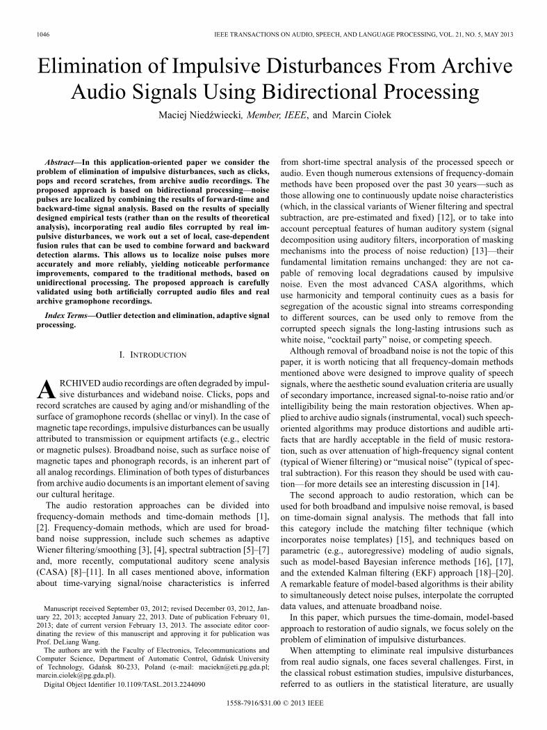
Fig. 1. Two fragments of an archive gramophone recording and the corre-sponding noise pulses denotes discrete time. In both cases the samplingrate was equal to 22.05 kHz.

modeled as isolated pulses of unity length, with a certainprobability of occurrence and a certain amplitude distribution(with variance much larger than signal variance) [21]. Eventhough audio signals corrupted by noise pulses generated inthis way sound very much like “old recordings,” detection ofreal impulsive disturbances based on such premises is usuallyfar from satisfactory. Real disturbances may last for several toseveral hundred sampling intervals and have different shapes,ranging from simple unimodal to complex multimodal (or evenoscillatory) patterns—see Fig. 1. In this paper most of theexperiments were performed on clean audio signals corruptedby impulsive disturbances extracted from old gramophonerecordings. Such a “disturbance transplantation” techniqueallows one to check reconstruction algorithms under realisticconditions. At the same time it gives insight into the “anatomy”of the reconstruction process, as the location and shape ofeach noise pulse is known exactly (allowing one to computeobjective performance measures).The second challenge is performance evaluation. No obvious

objective performance measure seems to exist that would allowone to evaluate and compare reconstruction results. Develop-ment of objective methods for quality assessment of speechand audio is a long-standing problem. The well-known PESQ(perceptual evaluation of speech quality) tool can be used toassess quality of narrow-band speech degraded by coding dis-tortions, transmission errors, packet loss, time-warping and en-vironmental noise [22]. However, it is reported unsuitable forquantifying quality of noise reduction algorithms [23]. Somemore recent results on the objective quality assessment problemare reported in [24], but impulsive disturbances are not amongthe five classes of audio degradation effects considered there.In case of impulsive disturbances the thing that really matters

is whether or not the applied reconstruction procedure producesaudible artifacts. Such artifacts may be caused by detection er-rors (undetected, or only partially detected, noise pulses), inter-polation errors (incorrectly interpolated samples), or by both.The most trustful quality measure is that based on subjectivelistening tests. Objective measures, although useful, should beused with caution. For example, when treated as the perfor-mance indicator, the number of undetected noise pulses may bemisleading as some of these disturbances may be not audible(audibility strongly depends on the local signal characteristics).Similarly, the number of false detections matters only if the in-terpolation that follows is of poor quality.Finally, the third challenge, particularly relevant in the case

of audio processing, is due to signal nonstationarity. Most ofthe existing detection and interpolation procedures are basedon the hypothesis of stationarity of the analyzed data. For thisreason they work satisfactorily when signal characteristicschange slowly over time (i.e., when the signal is “locally sta-tionary”), but may fail in the presence of their abrupt changes.“Unpredictable events”, such as emergence of new sounds, mayeasily fool the classical outlier detection algorithms. One of ourkey observations is that, unlike impulsive disturbances, suchforward-unpredictable events are often backward-predictable.This allows one to distinguish more precisely between naturalsounds and noise pulses.The main contribution of this paper is the demonstration that

impulsive disturbances can be eliminated more efficiently if theresults of forward-time signal analysis are combined with theanalogous results of its backward-time analysis. Such a bidirec-tional processing allows one to localize noise pulses more ac-curately and more reliably, yielding noticeable performance im-provements compared to unidirectional processing. To the bestof our knowledge, the idea of bidirectional processing was pre-viously exploited only once, in the paper of Canazza et al. [20].The method proposed there is based on combining restorationresults obtained independently by means of forward-time andbackward-time signal processing. The output signal is evaluatedas a linear (convex) combination of its forward and backwardcomponents. The weighting coefficients are computed based onthe local forward/backward prediction error statistics. Our ap-proach is different. Based on the results of tests, performed onreal audio signals, corrupted by real impulsive disturbances, wework out a set of local, case-dependent fusion rules that are fur-ther used to combine forward and backward detection alarms.Such an analysis is carried out prior to signal interpolation andallows one to “carve” detection alarms more carefully. This re-sults in better disturbance coverage statistics (smaller number ofshorter false alarms, smaller number of overlooked noise pulses,better front/back matching of noise pulses) and, in effect, inbetter restored sound quality.

II. UNIDIRECTIONAL PROCESSING

We will assume that the sampled audio signal has theform

(1)

where denotes normalized (dimension-less) discrete time, denotes the undistorted (clean) audio


signal, and is the sequence of noise pulses. No statisticalmodel of the disturbance (quantifying the frequency of occur-rence, length or shape of noise pulses) is assumed to be avail-able. By we will denote the pulse location function

The problem of elimination of impulsive disturbances can bedecomposed into two subproblems:1) Localization of noise pulses

2) Interpolation of samples regarded as outliersbased on the approved samples.

Most of the existing impulsive disturbance elimination tech-niques are based on autoregressive (AR) or sparse autoregres-sive (SAR) signal modeling, and model-based adaptive predic-tion: an on-line identification of the AR/SARmodel of the audiosignal is carried out and its results are used to predict new sam-ples from the old ones. If the magnitude of the prediction erroris too large (e.g., if it exceeds three standard deviations of itsnominal value), the sample is classified as an outlier and sched-uled for interpolation.

A. Approach Based on Classical AR Modeling

In this approach the sampled audio signal is representedby the following AR model of order

(2)

where are the so-called autoregressive coeffi-cients and denotes white driving noise. Model coeffi-cients are continuously updated using a parameter trackingalgorithm—such as exponentially weighted least squares(EWLS), least mean squares (LMS) or Kalman filter (KF)based [25], [26]—which yields . Denote by

the vector of autoregressive coefficients andby —the regression vector,made up of past signal values. The EWLS algorithm, knownof its good tracking capabilities, can be summarized as follows

(3)

where is the vector of parameter es-timates and , denotes the so-called forgetting con-stant, determining estimationmemory of the tracking algorithm.Recursive estimation of autoregressive coefficients is stoppedeach time a new noise pulse is detected. It is resumed when theprocess of reconstruction of the corrupted fragment is finished.Detection alarm starts at the instant : , when

the magnitude of the AR model-based one-step-ahead predic-

tion error exceeds times its estimated standard deviation (typ-ically )1

(4)

where

and denotes the local estimate of the driving noise vari-ance, obtained by means of averaging the recently observedsquared one-step-ahead prediction errors (after excludingoutliers).

The coefficient , denotes another forgetting con-stant which determines the estimation memory of the averagingalgorithm.The detection process is continued for multi-step-ahead pre-

dictions, i.e., the absolute values of the -step-ahead predictionerrors arechecked against the corresponding thresholds . Thealarm ends at the instant : , ifconsecutive prediction errors are sufficiently small, namely

(5)

or if the length of the detection alarm reaches the pre-scribed value . To avoid “accidental acceptances” ofcorrupted samples localized in the middle of long-lastingartifacts (such as the one depicted in Fig. 1), it is set

—even if for somevalue(s) of , the prediction error remains belowthe corresponding threshold. Detection alarms determined inthis way always form solid blocks of “ones” preceded andsucceeded by at least “zeros”. The quantity canbe obtained as a concatenation of one-step-ahead predictions,namely

(6)

where for . The variance of themulti-step prediction errors can be evaluated recursively usingthe following algorithm proposed by Stoica [27]

(7)

with initial conditions: and.

1The value corresponds to the well-known “three sigma” rule usedto detect outliers in Gaussian signals. Since audio signals are generally non-Gaussian, very often better results are obtained for .


When the detection process is finished, the sequence of irre-vocably distorted samples is inter-polated using the available signal model (2). The projection-based interpolation is based on samples preceding the missingblock, and samples succeeding the block—see Section III. In[19] all quantities needed to carry out the detection/interpola-tion process are evaluated by the extended Kalman filter (EKF).

B. Approach Based on Sparse AR Modeling

The procedure described above, based on AR modeling,often fails on speech signals, especially those with strongvoiced episodes. The reason is not difficult to find. Since voicedspeech sounds are formed by means of exciting the vocaltract (represented by the AR model) with a periodic train ofglottal air pulses, the outlier detector is prone to confuse pitchexcitation with noise pulses. Interestingly, the same effect canbe observed for audio signals with strong vocal components,and for purely instrumental music with contribution from somewind instruments, such as trumpet, saxophone or clarinet [28].The problem mentioned above can be overcome using sparseautoregressive modeling [29], [30]. The SARmodel of an audiosignal can be defined in the form

(8)

where the quantities and are chosen in such a waythat , where denotes the fundamentalperiod of the signal, e.g., in the case of speech signals the periodof pitch excitation (if present). Even though formally of order

, such a model is sparse as it contains onlynonzero coefficients.Sparse AR models capture both short-term correlations

[taken care of by the first component on the right-hand side of(8)] and long-term correlations [taken care of by the secondcomponent on the right hand side of (8)] of the analyzed timeseries.To better understand advantages of sparse modeling, consider

a signal governed by (2) in the case where is a periodictrain of pulses of arbitrary shape (rather than white noise). De-note by the period of such an external excitation. Since, understeady state conditions, the signal is also periodic with pe-riod , it obeys the following sparse model

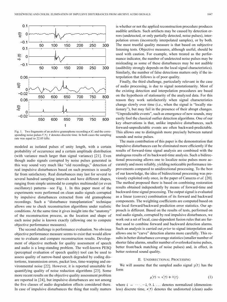
Note that such a model yields zero prediction errors at all timeinstants , including the moments of periodic input activity. Thisexplains good predictive capabilities of SARmodels in the pres-ence of mixed excitation (stochastic periodic)—provided, ofcourse, that the period is carefully chosen. Fig. 2 shows er-rors yielded by AR-based and SAR-based adaptive predictorsapplied to fragments of two audio signals: voiced speech andtrumpet music. In both cases the results obtained for the ARmodel of order 10 reveal the presence of a periodic excitation,which can be easily confused with noise pulses. When the samemodel is extended with just one long-term component

Fig. 2. Results obtained for two audio signals: voiced speech (three upperplots) and trumpet music (three lower plots). The corresponding plots show:the original audio signals (A), prediction errors yielded by the continuouslyupdated AR model (B), and prediction errors yielded by the continuouslyupdated SAR model (C). The order of the short-term part of both models is thesame and equal to .

and when is set to the estimated pitch period, signal predic-tions become much more accurate and prediction errors—freeof periodic excitation-related components.The main problem with the model (8) is that no identification

algorithms seem to exist that can guarantee its stability. Addi-tionally, since the order of the model is large (usuallyexceeding 100, even for moderate sampling rates), stability teststhat could eliminate unstable models are hardly practical. Sinceunstable models may lead to detection and interpolation errors(such as self-oscillatory interpolation artifacts), model stabilityis an important practical issue.The stability problem, mentioned above, can be easily solved

if the SAR model is sought in the following factorized form,widely used for predictive coding of speech, e.g., in CELPcoders [31], [32]

(9)

(10)

In the speech coding context, (9) describes the so-called formantfilter, characterized by formant coefficients , and (10)describes pitch filter, characterized by the pitch coefficient .The formant filter and the pitch filter form a cascade. Stabilityof the factorized model is guaranteed if both filters (formant andpitch) are stable, which can be easily achieved using appropriate


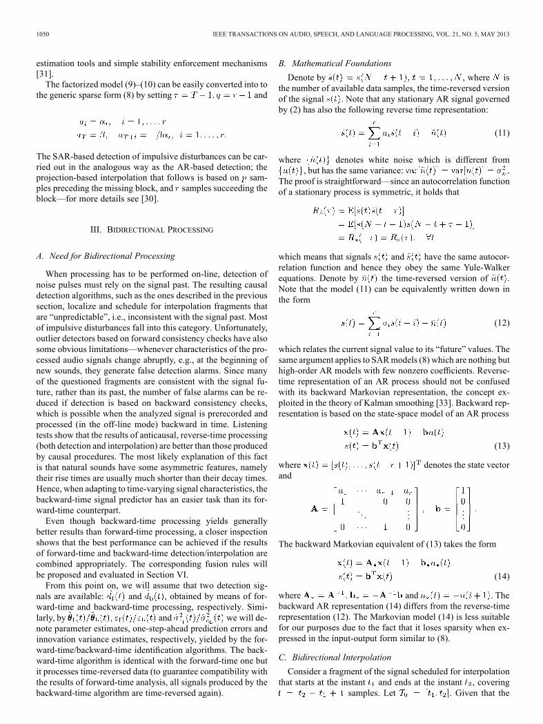
estimation tools and simple stability enforcement mechanisms[31].The factorized model (9)–(10) can be easily converted into to

the generic sparse form (8) by setting and

The SAR-based detection of impulsive disturbances can be car-ried out in the analogous way as the AR-based detection; theprojection-based interpolation that follows is based on sam-ples preceding the missing block, and samples succeeding theblock—for more details see [30].

III. BIDIRECTIONAL PROCESSING

A. Need for Bidirectional Processing

When processing has to be performed on-line, detection ofnoise pulses must rely on the signal past. The resulting causaldetection algorithms, such as the ones described in the previoussection, localize and schedule for interpolation fragments thatare “unpredictable”, i.e., inconsistent with the signal past. Mostof impulsive disturbances fall into this category. Unfortunately,outlier detectors based on forward consistency checks have alsosome obvious limitations—whenever characteristics of the pro-cessed audio signals change abruptly, e.g., at the beginning ofnew sounds, they generate false detection alarms. Since manyof the questioned fragments are consistent with the signal fu-ture, rather than its past, the number of false alarms can be re-duced if detection is based on backward consistency checks,which is possible when the analyzed signal is prerecorded andprocessed (in the off-line mode) backward in time. Listeningtests show that the results of anticausal, reverse-time processing(both detection and interpolation) are better than those producedby causal procedures. The most likely explanation of this factis that natural sounds have some asymmetric features, namelytheir rise times are usually much shorter than their decay times.Hence, when adapting to time-varying signal characteristics, thebackward-time signal predictor has an easier task than its for-ward-time counterpart.Even though backward-time processing yields generally

better results than forward-time processing, a closer inspectionshows that the best performance can be achieved if the resultsof forward-time and backward-time detection/interpolation arecombined appropriately. The corresponding fusion rules willbe proposed and evaluated in Section VI.From this point on, we will assume that two detection sig-

nals are available: and , obtained by means of for-ward-time and backward-time processing, respectively. Simi-larly, by and we will de-note parameter estimates, one-step-ahead prediction errors andinnovation variance estimates, respectively, yielded by the for-ward-time/backward-time identification algorithms. The back-ward-time algorithm is identical with the forward-time one butit processes time-reversed data (to guarantee compatibility withthe results of forward-time analysis, all signals produced by thebackward-time algorithm are time-reversed again).

B. Mathematical Foundations

Denote by , where isthe number of available data samples, the time-reversed versionof the signal . Note that any stationary AR signal governedby (2) has also the following reverse time representation:

(11)

where denotes white noise which is different from, but has the same variance: .

The proof is straightforward—since an autocorrelation functionof a stationary process is symmetric, it holds that

which means that signals and have the same autocor-relation function and hence they obey the same Yule-Walkerequations. Denote by the time-reversed version of .Note that the model (11) can be equivalently written down inthe form

(12)

which relates the current signal value to its “future” values. Thesame argument applies to SARmodels (8) which are nothing buthigh-order AR models with few nonzero coefficients. Reverse-time representation of an AR process should not be confusedwith its backward Markovian representation, the concept ex-ploited in the theory of Kalman smoothing [33]. Backward rep-resentation is based on the state-space model of an AR process

(13)

where denotes the state vectorand

. . ....

...

The backward Markovian equivalent of (13) takes the form

(14)

where and . Thebackward AR representation (14) differs from the reverse-timerepresentation (12). The Markovian model (14) is less suitablefor our purposes due to the fact that it loses sparsity when ex-pressed in the input-output form similar to (8).

C. Bidirectional Interpolation

Consider a fragment of the signal scheduled for interpolationthat starts at the instant and ends at the instant , covering

samples. Let . Given that the


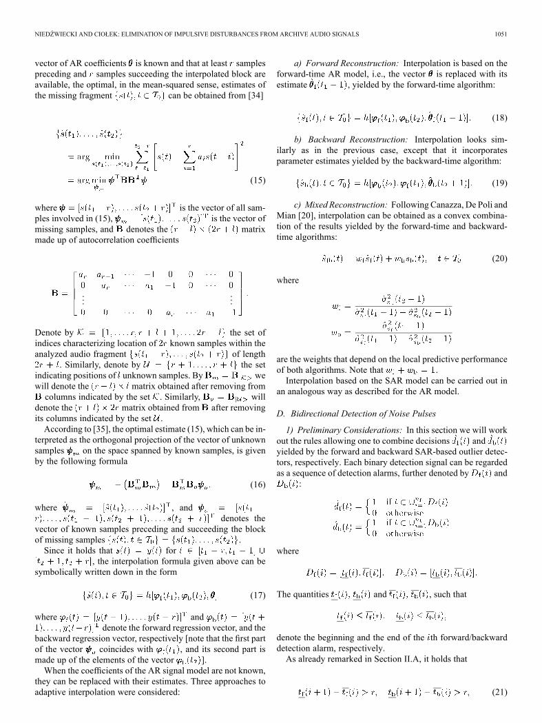
vector of AR coefficients is known and that at least samplespreceding and samples succeeding the interpolated block areavailable, the optimal, in the mean-squared sense, estimates ofthe missing fragment can be obtained from [34]

(15)

where is the vector of all sam-ples involved in (15), is the vector ofmissing samples, and denotes the matrixmade up of autocorrelation coefficients

......

Denote by the set ofindices characterizing location of known samples within theanalyzed audio fragment of length

. Similarly, denote by the setindicating positions of unknown samples. By wewill denote the matrix obtained after removing fromcolumns indicated by the set . Similarly, will

denote the matrix obtained from after removingits columns indicated by the set .According to [35], the optimal estimate (15), which can be in-

terpreted as the orthogonal projection of the vector of unknownsamples on the space spanned by known samples, is givenby the following formula

(16)

where , anddenotes the

vector of known samples preceding and succeeding the blockof missing samples .Since it holds that for

, the interpolation formula given above can besymbolically written down in the form

(17)

where anddenote the forward regression vector, and the

backward regression vector, respectively [note that the first partof the vector coincides with , and its second part ismade up of the elements of the vector ].When the coefficients of the AR signal model are not known,

they can be replaced with their estimates. Three approaches toadaptive interpolation were considered:

a) Forward Reconstruction: Interpolation is based on theforward-time AR model, i.e., the vector is replaced with itsestimate , yielded by the forward-time algorithm:

(18)

b) Backward Reconstruction: Interpolation looks sim-ilarly as in the previous case, except that it incorporatesparameter estimates yielded by the backward-time algorithm:

(19)

c) Mixed Reconstruction: Following Canazza, De Poli andMian [20], interpolation can be obtained as a convex combina-tion of the results yielded by the forward-time and backward-time algorithms:

(20)

where

are the weights that depend on the local predictive performanceof both algorithms. Note that .Interpolation based on the SAR model can be carried out in

an analogous way as described for the AR model.

D. Bidirectional Detection of Noise Pulses

1) Preliminary Considerations: In this section we will workout the rules allowing one to combine decisions andyielded by the forward and backward SAR-based outlier detec-tors, respectively. Each binary detection signal can be regardedas a sequence of detection alarms, further denoted by and

:

where

The quantities and , such that

denote the beginning and the end of the th forward/backwarddetection alarm, respectively.As already remarked in Section II.A, it holds that

(21)


i.e., the consecutive detection alarms are separated by at leastno-alarm decisions. This is the minimum distance allowing oneto decompose the problem of interpolation of blocks ofmissing samples into local interpolation tasks analyzedin the previous subsection. Note, however, that the analogousseparation between the forward and backward detection alarmsis not guaranteed, which means that when analyzed jointly, suchalarms may form complicated patterns. For this reason, forma-tion of the joint detection signal , based on the results ofboth forward-time and backward-time analysis, is a nontrivialtask.The simplest approach to combining results of forward-time

and backward-time detection is the one based on global decisionrules, such as the intersection rule

(22)

or the union rule

(23)

In the first case detection alarm is raised only when the sampleis questioned by both detectors, and in the second case—when itis questioned by at least one of the detectors. Preliminary testshave shown that neither of these rules works satisfactorily inpractice. The intersection rule is too conservative—it tends tooverlook many small noise pulses and produces underfitted (tooshort) detection alarms. The union rule is too liberal—it yieldsmany overfitted (too long) detection alarms which, after inter-polation, result in audible signal distortions.To avoid problems mentioned above, different configurations

of forward and backward detection alarms, further referred toas detection patterns, were divided into several classes and sub-classes. Each class was analyzed separately in order to deter-mine the best way of combining detection alarms. The final de-tection decision is a result of application of a certain number oflocal, case-dependent decision rules, called atomic fusion rules,rather than using a single global rule applicable to all cases.2) Preprocessing: Unlike artificially generated noise pulses,

real impulsive disturbances corrupting audio signals are rarelyconfined to isolated samples. Moreover, most of them have“soft” edges (the more so, the higher sampling rate) whichstems from the typical geometry of local damages of therecording medium (e.g., groove damages). The straightforwardconsequence of this fact is that detection alarms are seldomtriggered at the very beginning of noise pulses. This may leadto small but audible distortions of the reconstructed audiomaterial. Although detection delays can be reduced, or eveneliminated, by lowering the detection multiplier , i.e., bymaking the outlier detector more sensitive to “unpredictable”signal changes, the improvement comes at a price: low de-tection thresholds may dramatically increase the number andlength of detection alarms, causing the overall degradation ofthe results. An alternative solution, which works pretty wellin practice, is based on shifting back the beginning of eachdetection alarm (once determined) by a small fixed number ofsamples further denoted by . The resulting modified detectionalarms have the form

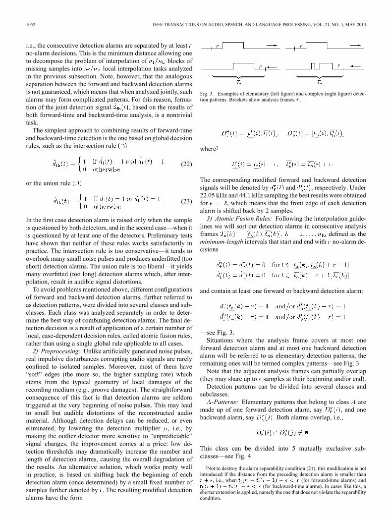
Fig. 3. Examples of elementary (left figure) and complex (right figure) detec-tion patterns. Brackets show analysis frames .

where2

The corresponding modified forward and backward detectionsignals will be denoted by and , respectively. Under22.05 kHz and 44.1 kHz sampling the best results were obtainedfor , which means that the front edge of each detectionalarm is shifted back by 2 samples.3) Atomic Fusion Rules: Following the interpolation guide-

lines we will sort out detection alarms in consecutive analysisframes defined as theminimum-length intervals that start and end with no-alarm de-cisions

and contain at least one forward or backward detection alarm:

—see Fig. 3.Situations where the analysis frame covers at most one

forward detection alarm and at most one backward detectionalarm will be referred to as elementary detection patterns; theremaining ones will be termed complex patterns—see Fig. 3.Note that the adjacent analysis frames can partially overlap

(they may share up to samples at their beginning and/or end).Detection patterns can be divided into several classes and

subclasses.-Patterns: Elementary patterns that belong to class are

made up of one forward detection alarm, say , and onebackward alarm, say . Both alarms overlap, i.e.,

This class can be divided into 5 mutually exclusive sub-classes—see Fig. 4

2Not to destroy the alarm separability condition (21), this modification is notintroduced if the distance from the preceding detection alarm is smaller than

, i.e., when (for forward-time alarms) and(for backward-time alarms). In cases like this, a

shorter extension is applied, namely the one that does not violate the separabilitycondition.


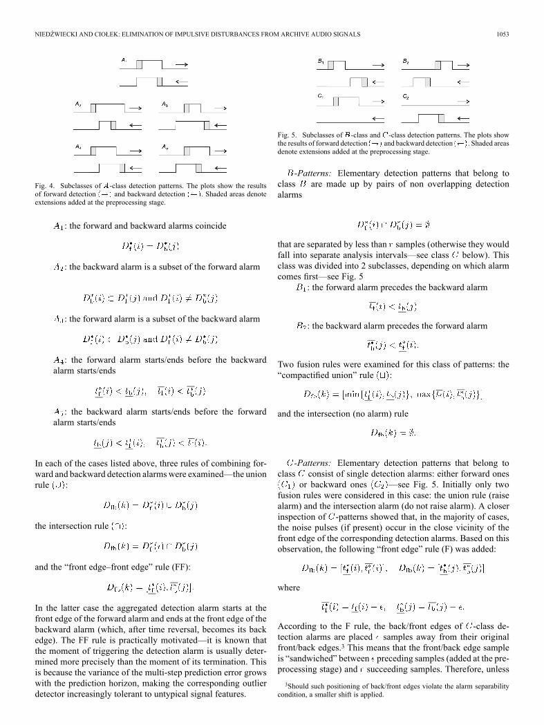
Fig. 4. Subclasses of -class detection patterns. The plots show the resultsof forward detection and backward detection . Shaded areas denoteextensions added at the preprocessing stage.

: the forward and backward alarms coincide

: the backward alarm is a subset of the forward alarm

: the forward alarm is a subset of the backward alarm

: the forward alarm starts/ends before the backwardalarm starts/ends

: the backward alarm starts/ends before the forwardalarm starts/ends

In each of the cases listed above, three rules of combining for-ward and backward detection alarms were examined—the unionrule :

the intersection rule :

and the “front edge–front edge” rule (FF):

In the latter case the aggregated detection alarm starts at thefront edge of the forward alarm and ends at the front edge of thebackward alarm (which, after time reversal, becomes its backedge). The FF rule is practically motivated—it is known thatthe moment of triggering the detection alarm is usually deter-mined more precisely than the moment of its termination. Thisis because the variance of the multi-step prediction error growswith the prediction horizon, making the corresponding outlierdetector increasingly tolerant to untypical signal features.

Fig. 5. Subclasses of -class and -class detection patterns. The plots showthe results of forward detection and backward detection . Shaded areasdenote extensions added at the preprocessing stage.

-Patterns: Elementary detection patterns that belong toclass are made up by pairs of non overlapping detectionalarms

that are separated by less than samples (otherwise they wouldfall into separate analysis intervals—see class below). Thisclass was divided into 2 subclasses, depending on which alarmcomes first—see Fig. 5

: the forward alarm precedes the backward alarm

: the backward alarm precedes the forward alarm

Two fusion rules were examined for this class of patterns: the“compactified union” rule :

and the intersection (no alarm) rule

-Patterns: Elementary detection patterns that belong toclass consist of single detection alarms: either forward ones

or backward ones —see Fig. 5. Initially only twofusion rules were considered in this case: the union rule (raisealarm) and the intersection alarm (do not raise alarm). A closerinspection of -patterns showed that, in the majority of cases,the noise pulses (if present) occur in the close vicinity of thefront edge of the corresponding detection alarms. Based on thisobservation, the following “front edge” rule (F) was added:

where

According to the F rule, the back/front edges of -class de-tection alarms are placed samples away from their originalfront/back edges.3 This means that the front/back edge sampleis “sandwiched” between preceding samples (added at the pre-processing stage) and succeeding samples. Therefore, unless

3Should such positioning of back/front edges violate the alarm separabilitycondition, a smaller shift is applied.


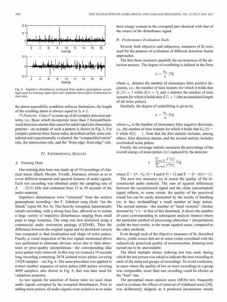
Fig. 6. Impulsive disturbances (extracted from archive gramophone record-ings) used for learning (upper plot) and validation (lower plot) of detection fu-sion rules.

the alarm separability condition enforces limitations, the lengthof the resulting alarm is always equal to .

-Patterns: Class is made up of all complex detection pat-terns, i.e., those which incorporate more than 2 forward/back-ward detection alarms that cannot be subdivided into elementarypatterns—an example of such a pattern is shown in Fig. 3. Forcomplex patterns three fusion rules, described earlier, were con-sidered and experimentally evaluated: the “compactified union”rule, the intersection rule, and the “front edge–front edge” rule.

IV. EXPERIMENTAL RESULTS

A. Training Data

Our training data base was made up of 10 recordings of clas-sical music (Bach, Mozart, Vivaldi, Smetana), chosen so as tocover different temporal and spectral features of audio signals.Each test recording was obtained under the sampling rate of

kHz and contained from 23 to 29 seconds of theaudio material.Impulsive disturbances were “extracted” from the archive

gramophone recording—the F. Schubert song (lied) “An dieMusik” (opus 88, No. 4). This heavily corrupted, harmonicallysimple recording, with a strong bass line, allowed us to isolatea large variety of impulsive disturbances ranging from smallpops to large scratches. The song was first declicked using acommercial audio restoration package (CEDAR). Then thedifference between the original signal and its declicked versionwas computed to find localization and shape of noise pulses.Finally, a visual inspection of the two signals mentioned abovewas performed to eliminate obvious errors due to false detec-tions or poor-quality interpolations—the corresponding fakenoise pulses were removed. In this way we created a 19 secondslong recording containing 2674 isolated noise pulses covering13428 samples—see Fig. 6. The same procedure was applied toextract another sequence of noise pulses (606 pulses covering4099 samples), also shown in Fig. 6, that was later used forvalidation purposes.As test signals for selection of fusion rules we used clean

audio signals corrupted by the extracted disturbances. Prior toadding noise pulses, all audio signals were scaled so as to make

their energy content in the corrupted part identical with that ofthe source of the disturbance signal.

B. Performance Evaluation Tools

Several, both objective and subjective, measures of fit wereused for the purpose of evaluation of different detection fusionapproaches.The first three measures quantify the accurateness of the de-

tection process. The degree of overfitting is defined in the form

%

where denotes the number of elementary false positive de-cisions, i.e., the number of time instants for which it holds that

while , and denotes the number of timeinstants for which it holds that (the accumulated lengthof all noise pulses).Similarly, the degree of underfitting is given by

%

where is the number of elementary false negative decisions,i.e., the number of time instants for which it holds thatwhile . Note that the first statistic includes, among

others, false detection alarms, and the second statistic includesoverlooked noise pulses.Finally, the coverage statistic measures the percentage of the

overall energy of noise pulses captured by the detector

%

where and and .The next two measures try to assess the quality of the re-

constructed audio material. The sum of squared differencesbetween the reconstructed signal and the clean (uncorrupted)signal reflects, to some extent, the quality of the perceivedsound but can be easily dominated by the results of handling(or, in fact, mishandling) a small number of large pulses.The second statistic—the number of “local victories” (furtherdenoted by ‘v’)—is free of this drawback. It shows the numberof cases (corresponding to subsequent analysis frames) wherethe particular method of processing (detection + interpolation)yields the best results, in the mean squared sense, compared tothe other methods.Even though each of the objective measures of fit, described

above, yields scores that are to some extent correlated with thesubjectively perceived quality of reconstruction, listening teststurned out to be unavoidable.The blind multiple choice ordering test was used, during

which the test person was asked to indicate the best recording ineach of the analyzed groups of recordings. To avoid confusion,in cases where the quality of two or more recordings in a groupwas comparable, more than one recording could be chosen asthe “best” one.The perceptual mean opinion score (MOS) test, frequently

used to evaluate the effects of removal of wideband noise [20],was deliberately skipped, as it produced inconsistent results


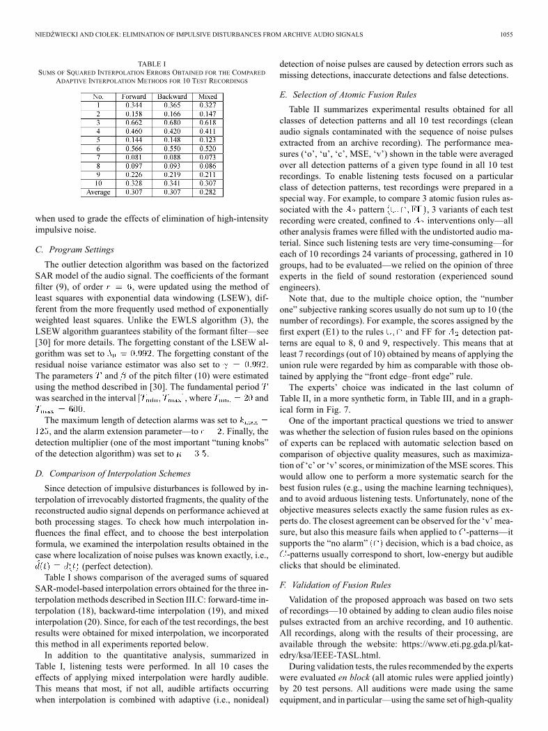
TABLE ISUMS OF SQUARED INTERPOLATION ERRORS OBTAINED FOR THE COMPARED

ADAPTIVE INTERPOLATION METHODS FOR 10 TEST RECORDINGS

when used to grade the effects of elimination of high-intensityimpulsive noise.

C. Program Settings

The outlier detection algorithm was based on the factorizedSAR model of the audio signal. The coefficients of the formantfilter (9), of order , were updated using the method ofleast squares with exponential data windowing (LSEW), dif-ferent from the more frequently used method of exponentiallyweighted least squares. Unlike the EWLS algorithm (3), theLSEW algorithm guarantees stability of the formant filter—see[30] for more details. The forgetting constant of the LSEW al-gorithm was set to . The forgetting constant of theresidual noise variance estimator was also set to .The parameters and of the pitch filter (10) were estimatedusing the method described in [30]. The fundamental periodwas searched in the interval , where and

.The maximum length of detection alarms was set to, and the alarm extension parameter—to . Finally, the

detection multiplier (one of the most important “tuning knobs”of the detection algorithm) was set to .

D. Comparison of Interpolation Schemes

Since detection of impulsive disturbances is followed by in-terpolation of irrevocably distorted fragments, the quality of thereconstructed audio signal depends on performance achieved atboth processing stages. To check how much interpolation in-fluences the final effect, and to choose the best interpolationformula, we examined the interpolation results obtained in thecase where localization of noise pulses was known exactly, i.e.,

(perfect detection).Table I shows comparison of the averaged sums of squared

SAR-model-based interpolation errors obtained for the three in-terpolation methods described in Section III.C: forward-time in-terpolation (18), backward-time interpolation (19), and mixedinterpolation (20). Since, for each of the test recordings, the bestresults were obtained for mixed interpolation, we incorporatedthis method in all experiments reported below.In addition to the quantitative analysis, summarized in

Table I, listening tests were performed. In all 10 cases theeffects of applying mixed interpolation were hardly audible.This means that most, if not all, audible artifacts occurringwhen interpolation is combined with adaptive (i.e., nonideal)

detection of noise pulses are caused by detection errors such asmissing detections, inaccurate detections and false detections.

E. Selection of Atomic Fusion Rules

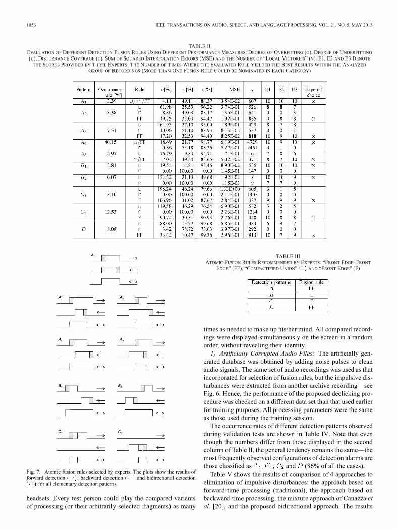
Table II summarizes experimental results obtained for allclasses of detection patterns and all 10 test recordings (cleanaudio signals contaminated with the sequence of noise pulsesextracted from an archive recording). The performance mea-sures (‘o’, ‘u’, ‘c’, MSE, ‘v’) shown in the table were averagedover all detection patterns of a given type found in all 10 testrecordings. To enable listening tests focused on a particularclass of detection patterns, test recordings were prepared in aspecial way. For example, to compare 3 atomic fusion rules as-sociated with the pattern , 3 variants of each testrecording were created, confined to interventions only—allother analysis frames were filled with the undistorted audio ma-terial. Since such listening tests are very time-consuming—foreach of 10 recordings 24 variants of processing, gathered in 10groups, had to be evaluated—we relied on the opinion of threeexperts in the field of sound restoration (experienced soundengineers).Note that, due to the multiple choice option, the “number

one” subjective ranking scores usually do not sum up to 10 (thenumber of recordings). For example, the scores assigned by thefirst expert (E1) to the rules and FF for detection pat-terns are equal to 8, 0 and 9, respectively. This means that atleast 7 recordings (out of 10) obtained by means of applying theunion rule were regarded by him as comparable with those ob-tained by applying the “front edge–front edge” rule.The experts’ choice was indicated in the last column of

Table II, in a more synthetic form, in Table III, and in a graph-ical form in Fig. 7.One of the important practical questions we tried to answer

was whether the selection of fusion rules based on the opinionsof experts can be replaced with automatic selection based oncomparison of objective quality measures, such as maximiza-tion of ‘c’ or ‘v’ scores, or minimization of theMSE scores. Thiswould allow one to perform a more systematic search for thebest fusion rules (e.g., using the machine learning techniques),and to avoid arduous listening tests. Unfortunately, none of theobjective measures selects exactly the same fusion rules as ex-perts do. The closest agreement can be observed for the ‘v’ mea-sure, but also this measure fails when applied to -patterns—itsupports the “no alarm” decision, which is a bad choice, as-patterns usually correspond to short, low-energy but audible

clicks that should be eliminated.

F. Validation of Fusion Rules

Validation of the proposed approach was based on two setsof recordings—10 obtained by adding to clean audio files noisepulses extracted from an archive recording, and 10 authentic.All recordings, along with the results of their processing, areavailable through the website: https://www.eti.pg.gda.pl/kat-edry/ksa/IEEE-TASL.html.During validation tests, the rules recommended by the experts

were evaluated en block (all atomic rules were applied jointly)by 20 test persons. All auditions were made using the sameequipment, and in particular—using the same set of high-quality


TABLE IIEVALUATION OF DIFFERENT DETECTION FUSION RULES USING DIFFERENT PERFORMANCE MEASURES: DEGREE OF OVERFITTING (O), DEGREE OF UNDERFITTING(U), DISTURBANCE COVERAGE (C), SUM OF SQUARED INTERPOLATION ERRORS (MSE) AND THE NUMBER OF “LOCAL VICTORIES” (V). E1, E2 AND E3 DENOTETHE SCORES PROVIDED BY THREE EXPERTS: THE NUMBER OF TIMES WHERE THE EVALUATED RULE YIELDED THE BEST RESULTS WITHIN THE ANALYZED

GROUP OF RECORDINGS (MORE THAN ONE FUSION RULE COULD BE NOMINATED IN EACH CATEGORY)

Fig. 7. Atomic fusion rules selected by experts. The plots show the results offorward detection , backward detection and bidirectional detection

for all elementary detection patterns.

headsets. Every test person could play the compared variantsof processing (or their arbitrarily selected fragments) as many

TABLE IIIATOMIC FUSION RULES RECOMMENDED BY EXPERTS: “FRONT EDGE–FRONT

EDGE” (FF), “COMPACTIFIED UNION” AND “FRONT EDGE” (F)

times as needed to make up his/her mind. All compared record-ings were displayed simultaneously on the screen in a randomorder, without revealing their identity.1) Artificially Corrupted Audio Files: The artificially gen-

erated database was obtained by adding noise pulses to cleanaudio signals. The same set of audio recordings was used as thatincorporated for selection of fusion rules, but the impulsive dis-turbances were extracted from another archive recording—seeFig. 6. Hence, the performance of the proposed declicking pro-cedure was checked on a different data set than that used earlierfor training purposes. All processing parameters were the sameas those used during the training session.The occurrence rates of different detection patterns observed

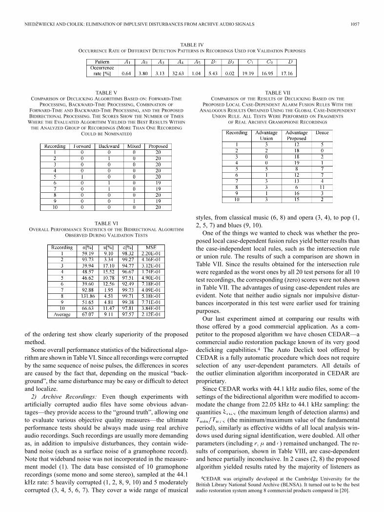
during validation tests are shown in Table IV. Note that eventhough the numbers differ from those displayed in the secondcolumn of Table II, the general tendency remains the same—themost frequently observed configurations of detection alarms arethose classified as and (86% of all the cases).Table V shows the results of comparison of 4 approaches to

elimination of impulsive disturbances: the approach based onforward-time processing (traditional), the approach based onbackward-time processing, the mixture approach of Canazza etal. [20], and the proposed bidirectional approach. The results


TABLE IVOCCURRENCE RATE OF DIFFERENT DETECTION PATTERNS IN RECORDINGS USED FOR VALIDATION PURPOSES

TABLE VCOMPARISON OF DECLICKING ALGORITHMS BASED ON: FORWARD-TIME

PROCESSING, BACKWARD-TIME PROCESSING, COMBINATION OF

FORWARD-TIME AND BACKWARD-TIME PROCESSING, AND THE PROPOSEDBIDIRECTIONAL PROCESSING. THE SCORES SHOW THE NUMBER OF TIMESWHERE THE EVALUATED ALGORITHM YIELDED THE BEST RESULTS WITHINTHE ANALYZED GROUP OF RECORDINGS (MORE THAN ONE RECORDING

COULD BE NOMINATED)

TABLE VIOVERALL PERFORMANCE STATISTICS OF THE BIDIRECTIONAL ALGORITHM

OBSERVED DURING VALIDATION TESTS

of the ordering test show clearly superiority of the proposedmethod.Some overall performance statistics of the bidirectional algo-

rithm are shown in Table VI. Since all recordings were corruptedby the same sequence of noise pulses, the differences in scoresare caused by the fact that, depending on the musical “back-ground”, the same disturbance may be easy or difficult to detectand localize.2) Archive Recordings: Even though experiments with

artificially corrupted audio files have some obvious advan-tages—they provide access to the “ground truth”, allowing oneto evaluate various objective quality measures—the ultimateperformance tests should be always made using real archiveaudio recordings. Such recordings are usually more demandingas, in addition to impulsive disturbances, they contain wide-band noise (such as a surface noise of a gramophone record).Note that wideband noise was not incorporated in the measure-ment model (1). The data base consisted of 10 gramophonerecordings (some mono and some stereo), sampled at the 44.1kHz rate: 5 heavily corrupted (1, 2, 8, 9, 10) and 5 moderatelycorrupted (3, 4, 5, 6, 7). They cover a wide range of musical

TABLE VIICOMPARISON OF THE RESULTS OF DECLICKING BASED ON THE

PROPOSED LOCAL CASE-DEPENDENT ALARM FUSION RULES WITH THEANALOGOUS RESULTS OBTAINED USING THE GLOBAL CASE-INDEPENDENT

UNION RULE. ALL TESTS WERE PERFORMED ON FRAGMENTSOF REAL ARCHIVE GRAMOPHONE RECORDINGS

styles, from classical music (6, 8) and opera (3, 4), to pop (1,2, 5, 7) and blues (9, 10).One of the things we wanted to check was whether the pro-

posed local case-dependent fusion rules yield better results thanthe case-independent local rules, such as the intersection ruleor union rule. The results of such a comparison are shown inTable VII. Since the results obtained for the intersection rulewere regarded as the worst ones by all 20 test persons for all 10test recordings, the corresponding (zero) scores were not shownin Table VII. The advantages of using case-dependent rules areevident. Note that neither audio signals nor impulsive distur-bances incorporated in this test were earlier used for trainingpurposes.Our last experiment aimed at comparing our results with

those offered by a good commercial application. As a com-petitor to the proposed algorithm we have chosen CEDAR—acommercial audio restoration package known of its very gooddeclicking capabilities.4 The Auto Declick tool offered byCEDAR is a fully automatic procedure which does not requireselection of any user-dependent parameters. All details ofthe outlier elimination algorithm incorporated in CEDAR areproprietary.Since CEDAR works with 44.1 kHz audio files, some of the

settings of the bidirectional algorithm were modified to accom-modate the change from 22.05 kHz to 44.1 kHz sampling: thequantities (the maximum length of detection alarms) and

(the minimum/maximum value of the fundamentalperiod), similarly as effective widths of all local analysis win-dows used during signal identification, were doubled. All otherparameters (including and ) remained unchanged. The re-sults of comparison, shown in Table VIII, are case-dependentand hence partially inconclusive. In 2 cases (2, 8) the proposedalgorithm yielded results rated by the majority of listeners as

4CEDAR was originally developed at the Cambridge University for theBritish Library National Sound Archive (BLNSA). It turned out to be the bestaudio restoration system among 8 commercial products compared in [20].


TABLE VIIICOMPARISON OF THE RESULTS YIELDED BY THE AUTO DECLICK CEDARTOOL WITH THOSE PRODUCED BY THE PROPOSED BIDIRECTIONALALGORITHM. ALL TESTS WERE PERFORMED ON FRAGMENTS

OF REAL ARCHIVE GRAMOPHONE RECORDINGS

better than those produced by CEDAR, in one case (10) thescores were identical, and in the remaining 7 cases CEDAR wasrated higher. All listeners stressed, however, that the differenceswere subtle—note a relatively large number of neutral decisions(almost 25%).Even though the overall rating of CEDAR was higher, it

should be noted that the proposed algorithm was run withdefault settings. In particular, no attempt was made to optimizeits performance by selecting the detection multiplier , morecarefully. We have noted that in many cases considerably betterresults can be obtained when is trimmed to the particularrecording at hand. This leaves the room for further improve-ments. Automatic selection of will be a subject of our furtherresearch.

G. Universality Versus Specificity

Validation tests have shown that even though trained to per-form well on a particular realization of impulsive disturbances,the proposed fusion rules are pretty universal, i.e., they worksatisfactorily when applied to a large variety of archive record-ings. It should be stressed, however, that rather than the concreteset of decision rules, the main contribution of this paper is theprocedure (including preparation of the test data files) for theirselection and validation. Applying this procedure to more spe-cialized training data, one can easily arrive at new rules, better“matched” to the particular problem at hand, e.g., to a particularclass of audio recordings and/or disturbances.

V. CONCLUSION

It was shown that impulsive disturbances can be eliminatedfrom archive audio recordings more efficiently if the results oftraditional, forward-time outlier detection are combined withthe analogous results of backward-time detection. The set oflocal fusion rules, allowing one to combine forward/backwarddetection alarms, was established and validated experimentally,using both artificially corrupted audio files and real archivegramophone recordings. The new bidirectional approach of-fers performance improvements compared to the classicalunidirectional approach and yields results comparable withthose produced by the state-of-the-art commercial declickingsoftware.

REFERENCES

[1] S. V. Vaseghi, Advanced Signal Processing and Digital Noise Reduc-tion. New York, NY, USA: Wiley, 1996.

[2] J. S. Godsill and J. P. W. Rayner, Digital Audio Restoration. Berlin,Germany: Springer-Verlag, 1998.

[3] J. Lim and A. Oppenheim, “All-pole modeling of degraded speech,”IEEE Trans. Acoust., Speech, Signal Process., vol. ASSP-26, no. 3,pp. 197–210, Jun. 1978.

[4] D. M. Y. Ephraim, “Speech enhancement using a minimummean-square error short-time spectral amplitude estimator,” IEEETrans. Acoust., Speech, Signal Process., vol. ASSP-32, no. 6, pp.1109–1121, Jun. 1984.

[5] S. Böll, “Suppression of acoustic noise in speech using spectral sub-traction,” IEEE Trans. Acoust., Speech, Signal Process., vol. ASSP-27,no. 2, pp. 113–120, Apr. 1979.

[6] R. J. McAulay and M. L. Malpass, “Speech enhancement using a softdecision noise suppression filter,” IEEE Trans. Acoust., Speech, SignalProcess., vol. ASSP-28, no. 2, pp. 137–145, Apr. 1980.

[7] P. Vary, “Noise suppression by spectral amplitude estimation—Mecha-nism and theoretical limits,” Signal Process., vol. 8, pp. 387–400, 1985.

[8] D. F. Rosenthal and H. G. Okuno, Computational Auditory Scene Anal-ysis. Mahwah, NJ, USA: Lawrence Erlbaum, 1998.

[9] D. L. Wang and G. J. Brown, “Separation of speech from interferingsounds based on oscillatory correlations,” IEEE Trans. Neural Netw.,vol. 10, no. 3, pp. 684–697, May 1999.

[10] G. Hu and D. L. Wang, “Monaural speech segregation based on pitchtracking and amplitude modulation,” IEEE Trans. Neural Netw., vol.15, no. 5, pp. 1135–1150, Sep. 2004.

[11] D. L. Wang and G. J. Brown, Computational Auditory Scene Anal-ysis: Principles, Algorithms and Applications. New York, NY, USA:Wiley, 2006.

[12] R. Martin, “Noise power spectral density estimation based on optimalsmoothing and minimum statistics,” IEEE Trans. Speech AudioProcess., vol. 9, no. 5, pp. 504–512, Jul. 2001.

[13] D. E. Tsoukalas, J. N. Mourjopoulos, and G. Kokkinakis, “Speech en-hancement based on audible noise suppression,” IEEE Trans. SpeechAudio Process., vol. 5, no. 6, pp. 497–513, Nov. 1997.

[14] S. Canazza, G. Coraddu, G. De Poli, and G. A. Mian, “Objective andsubjective comparison of audio restoration systems,” in Proc. Int. Cul-tural Heritage Informatics Meeting, ICHIM’01, 2001, pp. 273–281.

[15] S. V. Vaseghi and R. Frayling-Cork, “Restoration of old gramophonerecordings,” J. Audio Eng. Soc., vol. 40, pp. 791–801, 1992.

[16] S. J. Godsill and P. J. W. Rayner, “A Bayesian approach to the restora-tion of degraded audio signals,” IEEE Trans. Speech Audio Process.,vol. 3, no. 4, pp. 267–278, Jul. 1995.

[17] S. J. Godsill and P. J. W. Rayner, “Statistical reconstruction and anal-ysis of autoregressive signals in impulsive noise using the Gibbs sam-pler,” IEEE Trans. Speech, Audio Process., vol. 6, no. 4, pp. 352–372,Jul. 1995.

[18] M. Niedźwiecki and K. Cisowski, “Adaptive scheme for eliminationof broadband noise and impulsive disturbances from audio signals,” inProc. Quatrozieme Colloque GRETSI, 1993, pp. 519–522.

[19] M. Niedźwiecki and K. Cisowski, “Adaptive scheme for eliminationof broadband noise and impulsive disturbances from AR and ARMAsignals,” IEEE Trans. Signal Process., vol. 44, no. 3, pp. 528–537,Mar.1996.

[20] S. Canazza, G. De Poli, and G. A. Mian, “Restoration of audiodocuments by means of extended Kalman filter,” IEEE Trans. Audio,Speech, Lang. Process., vol. 41, no. 6, pp. 1107–1115, Aug. 2010.

[21] A. M. Zoubir, V. Koivunen, Y. Chakhchoukh, and M. Muma, “Robustestimation in signal processing,” IEEE Signal Process. Mag., vol. 29,no. 4, pp. 61–80, Jul. 2012.

[22] Perceptual evaluation of speech quality (PESQ): objective method forend-to-end speech quality assessment of narrow band telephone net-works and speech codecs, ITU-T Rec. P.862, Int. Telecomm. Union,Geneva, Switzerland, 2005.

[23] J. G. Beerends, A. Hekstra, A. Rix, and M. Hollier, “Perceptual eval-uation of speech quality (PESQ), the new ITU standard for end-to-endspeech quality assessment, Part II—Psychoacoustic model,” J. AudioEng. Soc., vol. 50, pp. 765–778, 2002.

[24] P. A. A. Esqef, L. W. P. Biscainho, L. O. Nunes, B. Lee, A. Said, T.Kalker, and R. W. Schafer, “Quality assessment of audio: Increasingapplicability scope of objective methods via prior identification ofimpairment type,” in Proc. IEEE Int. Workshop Multimedia SignalProcess., 2009, pp. 1–6.


[25] S. Haykin, Adaptive Filter Theory. Englewood Cliffs, NJ, USA:Prentice-Hall, 1979.

[26] M. Niedźwiecki, Identification of Time-Varying Processes. NewYork, NY, USA: Wiley, 2001.

[27] P. Stoica, “Multistep prediction of autoregressive signals,” Electron.Lett., vol. 29, pp. 554–555, 1993.

[28] J. Wolfe, M. Garnier, and J. Smith, “Vocal tract resonances in speech,singing, and playing musical instruments,” HFSP J., vol. 3, pp. 6–23,2009.

[29] S. V. Vaseghi and P. J. W. Rayner, “Detection and suppression of im-pulsive noise in speech communication systems,” IEE Proc., vol. 137,pp. 38–46, 1990.

[30] M. Niedźwiecki and M. Ciołek, “Elimination of clicks from archivespeech signals using sparse autoregressive modeling,” in Proc. 20thEur. Signal Process. Conf., Bucharest, Romania, 2012.

[31] P. R. Ramachandran and P. Kabal, “Stability and performance analysisof pitch filters in speech coders,” IEEE Trans. Acoust., Speech, SignalProcess., vol. ASSP-35, no. 7, pp. 937–946, Jul. 1987.

[32] P. R. Ramachandran and P. Kabal, “Pitch prediction filters in speechcoding,” IEEE Trans. Acoust., Speech, Signal Process., vol. 37, no. 4,pp. 467–478, Apr. 1989.

[33] M.Niedźwiecki, “Locally adaptive cooperative Kalman smoothing andits application to identification of nonstationary stochastic systems,”IEEE Trans. Signal Process., vol. 60, no. 1, pp. 48–59, Jan. 2012.

[34] F. Lewis, Optimal Estimation. New York, NY, USA: Wiley, 1986.[35] M. Niedźwiecki, “Statistical reconstruction of multivariate time se-

ries,” IEEE Trans. Signal Process., vol. 41, no. 1, pp. 451–457, Jan.1993.

Maciej Niedźwiecki (M’07) was born in Poznań,Poland in 1953. He received the M.Sc. and Ph.D.degrees from the Technical University of Gdańsk,Gdańsk, Poland and the Dr.Hab. (D.Sc.) degreefrom the Technical University of Warsaw, Warsaw,Poland, in 1977, 1981 and 1991, respectively. Hespent three years as a Research Fellow with theDepartment of Systems Engineering, AustralianNational University, 1986–1989. In 1990–1993,he served as a Vice Chairman of Technical Com-mittee on Theory of the International Federation

of Automatic Control (IFAC). He is currently Associate Editor for IEEETRANSACTIONS ON SIGNAL PROCESSING, a member of the IFAC committees onModeling, Identification and Signal Processing and on Large Scale ComplexSystems, and a member of the Automatic Control and Robotics Committeeof the Polish Academy of Sciences (PAN). He is the author of the bookIdentification of Time-varying Processes (Wiley, 2000).He works as a Professor and Head of the Department of Automatic Control,

Faculty of Electronics, Telecommunications and Computer Science, GdańskUniversity of Technology. His main areas of research interests include systemidentification, statistical signal processing and adaptive systems.

Marcin Ciołek received the M.Sc. degree in au-tomatic control from the Gdańsk University ofTechnology, Gdańsk, Poland, in 2010, where iscurrently pursuing the Ph.D. degree. Since 2011,he has been working as an Assistant Professor inthe Department of Automatic Control, Faculty ofElectronics, Telecommunications and ComputerScience, Gdańsk University of Technology. Hisprofessional interests include speech, music andbiomedical signal processing.

Date post:	03-Dec-2016
Category:	Documents
Upload:	marcin
View:	214 times
Download:	0 times

Elimination of Impulsive Disturbances From Archive Audio Signals Using Bidirectional Processing

Documents