www.mve.com Elliptical Fault Flow Elliptical Fault Flow provides a new way to model and restore faults with variable offsets using Move™. This new kinematic algorithm was created by Midland Valley, and is accessed through the 2D Move-on-Fault and Horizon from Fault toolboxes in Move2017.2. Elliptical Fault Flow is the first kinematic algorithm to fully incorporate non-uniform fault displacement profiles and gradients; as a result, the algorithm significantly expands the range of faulting styles that can be modelled using 2D Move-on-Fault algorithms. As with other 2D Move-on-Fault algorithms, Elliptical Fault Flow predicts fault-related deformation for a given fault shape and offset using mathematical relationships derived from empirical field data (Watterson 1986; Barnett et al. 1987; Walsh & Watterson 1988; Gibson et al. 1989). In Move, the interface for the Elliptical Fault Flow algorithm has been optimized to allow the validity of interpretations to be quickly assessed, and to ensure that faults with non-uniform fault displacement profiles and gradients can be restored as easily as possible. Faults with non-uniform displacement profiles and gradients are well documented; with numerous field studies identifying faults with offsets that decrease in all directions away from a point of maximum displacement (e.g. Nixon et al. 2014). Typically, these faults cannot be modelled or restored with existing 2D Move-on-Fault algorithms, which require fault offsets to remain constant or increase with depth (Figure 1a). Moreover, existing 2D Move-on-Fault algorithms only predict fault-related folding at bends in faults and do not reproduce the drag folding associated with along-fault variations in offset (Figure 1b). These fault systems often form hydrocarbon traps and can influence fluid flow within reservoirs. Elliptical Fault Flow will allow the development of these fault systems to be better understood, as well as providing geologists with a new approach to quickly assess the validity of the surrounding interpretation. In this Move feature, we describe the methodology of Elliptical Fault Flow and the impact of different input parameters. We then use Elliptical Fault Flow to forward model fault-related deformation to aid seismic interpretation and to better understand deformation in an extensional system. Finally, we use Elliptical Fault Flow to restore a normal fault, which has experienced multiple phases of activity. Figure 1. Forward models of normal fault using: (a) inclined Simple Shear with approximately uniform displacements in the hanging wall; (b) Elliptical Fault Flow, with displacements that decrease away from the centre of the fault. a) b)
Transcript
www.mve.com
Elliptical Fault Flow Elliptical Fault Flow provides a new way to model and restore faults with variable offsets using Move™. This new kinematic algorithm was created by Midland Valley, and is accessed through the 2D Move-on-Fault and Horizon from Fault toolboxes in Move2017.2. Elliptical Fault Flow is the first kinematic algorithm to fully incorporate non-uniform fault displacement profiles and gradients; as a result, the algorithm significantly expands the range of faulting styles that can be modelled using 2D Move-on-Fault algorithms. As with other 2D Move-on-Fault algorithms, Elliptical Fault Flow predicts fault-related deformation for a given fault shape and offset using mathematical relationships derived from empirical field data (Watterson 1986; Barnett et al. 1987; Walsh & Watterson 1988; Gibson et al. 1989). In Move, the interface for the Elliptical Fault Flow algorithm has been optimized to allow the validity of interpretations to be quickly assessed, and to ensure that faults with non-uniform fault displacement profiles and gradients can be restored as easily as possible. Faults with non-uniform displacement profiles and gradients are well documented; with numerous field studies identifying faults with offsets that decrease in all directions away from a point of maximum displacement (e.g. Nixon et al. 2014). Typically, these faults cannot be modelled or restored with existing 2D Move-on-Fault algorithms, which require fault offsets to remain constant or increase with depth (Figure 1a). Moreover, existing 2D Move-on-Fault algorithms only predict fault-related folding at bends in faults and do not reproduce the drag folding associated with along-fault variations in offset (Figure 1b). These fault systems often form hydrocarbon traps and can influence fluid flow within reservoirs. Elliptical Fault Flow will allow the development of these fault systems to be better understood, as well as providing geologists with a new approach to quickly assess the validity of the surrounding interpretation. In this Move feature, we describe the methodology of Elliptical Fault Flow and the impact of different input parameters. We then use Elliptical Fault Flow to forward model fault-related deformation to aid seismic interpretation and to better understand deformation in an extensional system. Finally, we use Elliptical Fault Flow to restore a normal fault, which has experienced multiple phases of activity.
Figure 1. Forward models of normal fault using: (a) inclined Simple Shear with approximately uniform displacements in the hanging wall; (b) Elliptical Fault Flow, with displacements that decrease away from the centre of the fault.
Methodology Elliptical Fault Flow calculates the displacement field around a fault using the spatial extent of fault–related deformation, the maximum amount of fault offset or slip, and two published relationships to define the decrease in displacement away from a maxima (Watterson 1986; Barnett et al. 1987). This displacement field describes how particles have moved in the hanging wall and footwall of the fault in response to fault slip. Initially, the algorithm calculates the magnitudes for the displacement field as factors between 0 and 1; this displacement field is determined by multiplying the results from three equations which control: (1) the displacement profile along the fault surface; (2) the decrease in displacements away from the fault; and (3) the division of displacement between the hanging wall and footwall. The equations to calculate the initial displacement field use an elliptical shape that mirrors the geometry of the fault. This shape defines the spatial extent of fault-related deformation (Figure 2). The dimensions of the elliptical shape are controlled by the distance between the point of maximum offset and the fault tip (defined as 𝑄𝑄), and a user-defined length of the ellipse axis perpendicular to the fault (𝑅𝑅). These distances would typically be determined from inflection points in fault-related folds interpreted from seismic data or field observations. In Move, the dimensions of the elliptical shape are specified using the Up, Down, Left and Right options in the Displacement Radius portion of the Movement sheet.
Figure 2. Illustration showing key parameters used to calculate displacement with Elliptical Fault Flow for: (a) a planar normal fault; (b) a concave upward curved, normal fault. Black dash lines represent the spatial extent of fault-related deformation. Area around faults colour mapped for the normalised displacement value, including 20% footwall movement.
The first equation used to define the initial displacement field calculates the displacement profile along the fault surface. By default, this equation is based on the idealised fault slip profile published by Watterson (1986) and Walsh and Watterson (1988):
𝑠𝑠𝑛𝑛 = 2 ���(1+𝑄𝑄𝑛𝑛)2
�2− 𝑄𝑄𝑛𝑛2 � (1 − 𝑄𝑄𝑛𝑛) [1]
where, 𝑄𝑄𝑛𝑛 is the distance between a specific point along the fault from the point of maximum offset, normalised with respect to the distance between the point of maximum offset and the fault tip (𝑄𝑄) (Figure 2). For any given point around the fault, 𝑄𝑄𝑛𝑛 can be calculated by identifying the nearest point on the fault plane, measuring the distance between the nearest point on the fault plane and the point of maximum offset (Figure 2), and then dividing this by 𝑄𝑄 to give a value between 0 and 1. The second equation used to define the initial displacement field considers the decrease in the magnitude of displacement away from the fault. In Elliptical Fault Flow, the rate of decrease in displacement away from the fault is calculated using the equation published by Barnett et al. (1987): (1 − 𝑑𝑑𝑛𝑛)2 + (1 −𝑚𝑚𝑛𝑛)2 = 1 [2] where, 𝑑𝑑𝑛𝑛is the distance away from fault (𝑑𝑑𝑗𝑗 in Figure 2), normalised with respect to the length of the ellipse axis perpendicular to the fault (R), and 𝑚𝑚𝑛𝑛 is the magnitude of displacement associated with faulting. The third equation used to define the initial displacement field considers differences in the magnitude of displacements between the footwall and hanging wall. Elliptical Fault Flow is the only 2D Move-on-Fault algorithm to consider the effects of footwall upwarping, which is well documented in field data (e.g. Resor 2008). The amount of footwall movement is controlled by the Percentage of Footwall Movement, 𝑚𝑚𝐹𝐹𝐹𝐹, which can either be specified as a percentage (0% being no footwall movement, and 100% being no hanging wall movement), or calculated from the dip of the fault (𝜃𝜃) using the equation provided in Gibson et al. (1989) for faults with dips >30°: 𝑚𝑚𝐹𝐹𝐹𝐹 = 2𝜃𝜃
3− 10 [3]
The value for the initial displacement field for any given point in the footwall is calculated by multiplying 𝑠𝑠𝑛𝑛 and 𝑚𝑚𝑛𝑛 from equations [1] and [2], and the footwall movement percentage (𝑚𝑚𝐹𝐹𝐹𝐹); in the hanging wall, the values are determined by multiplying 𝑠𝑠𝑛𝑛 and 𝑚𝑚𝑛𝑛 from equations [1] and [2], with the hanging wall movement percentage (100% − 𝑚𝑚𝐹𝐹𝐹𝐹). The initial displacement field is then multiplied by the maximum amount of slip on the fault to determine the absolute magnitude of displacement.
By default, the direction of the displacement vectors will be orientated parallel to fault. However, this can be adjusted to produce curved particle pathways, which are similar to the pathways obtained from many geomechanical methods, such as Fault Response Modelling. Curved particle pathways can be considered using the Maximum Deflection Angle, which can be specified in the Movement sheet of the 2D Move-on-Fault and Horizons from Fault toolboxes. This Maximum Deflection Angle represents the maximum possible difference in degrees between the direction of the calculated displacement vectors and the dip of the fault. If the Maximum Deflection Angle is set to 0 degrees, everything moves parallel to the fault. If the Maximum Deflection Angle is set to be >0 degrees, the defined angle is multiplied by a deflection factor; a number between 0 and 1 that is calculated from the elliptical shape defining the spatial extent of fault-related deformation and the magnitudes in the initial displacement field (Figure 3). The basis for the deflection factor is determined from the ratio of arc lengths along the ellipse (𝑑𝑑𝑎𝑎 and 𝑑𝑑𝑏𝑏 in Figure 3). In every quarter of the ellipse, the maximum deflection factor occurs when 𝑑𝑑𝑎𝑎 and 𝑑𝑑𝑏𝑏 are equal, with the value decreasing linearly away from this point. As a result, deflection factors are always zero at the fault plane and along the axis of the ellipse perpendicular to the fault, which is centred on the point of maximum fault offset. This ratio is then multiplied by the magnitude values from the initial displacement field, resulting in particle pathways having greater obliquity to the fault in areas with higher displacement magnitudes.
Figure 3. Illustration showing the normalised deflection factor and maximum possible deflection of movement trajectories (Maximum Deflection Angles of 90 degrees) around: (a) a planar normal fault; (b) a concave upward curved, normal fault.
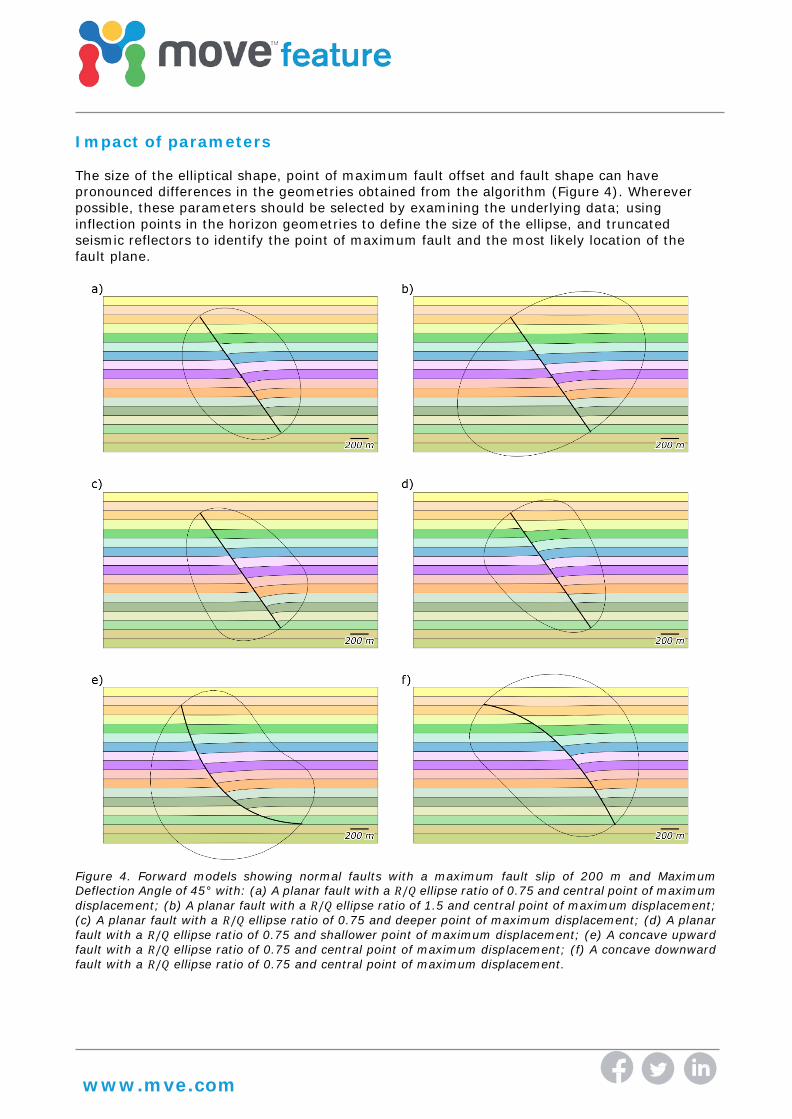
Impact of parameters The size of the elliptical shape, point of maximum fault offset and fault shape can have pronounced differences in the geometries obtained from the algorithm (Figure 4). Wherever possible, these parameters should be selected by examining the underlying data; using inflection points in the horizon geometries to define the size of the ellipse, and truncated seismic reflectors to identify the point of maximum fault and the most likely location of the fault plane.
Figure 4. Forward models showing normal faults with a maximum fault slip of 200 m and Maximum Deflection Angle of 45° with: (a) A planar fault with a 𝑅𝑅/𝑄𝑄 ellipse ratio of 0.75 and central point of maximum displacement; (b) A planar fault with a 𝑅𝑅/𝑄𝑄 ellipse ratio of 1.5 and central point of maximum displacement; (c) A planar fault with a 𝑅𝑅/𝑄𝑄 ellipse ratio of 0.75 and deeper point of maximum displacement; (d) A planar fault with a 𝑅𝑅/𝑄𝑄 ellipse ratio of 0.75 and shallower point of maximum displacement; (e) A concave upward fault with a 𝑅𝑅/𝑄𝑄 ellipse ratio of 0.75 and central point of maximum displacement; (f) A concave downward fault with a 𝑅𝑅/𝑄𝑄 ellipse ratio of 0.75 and central point of maximum displacement.
Forward modelling applications Forward modelling using 2D Move-on-Fault algorithms allows the structural validity of interpretations to be tested and evaluated. The aim of this forward modelling is usually to reproduce the position and shapes of horizons around interpreted faults; if the modelled horizons cannot be made to match the interpretation, it could suggest that the interpretation is incorrect and needs to be revised. In other instances, forward modelling can provide information about the tectonic evolution of a region or the development of hydrocarbon traps. The inclusion of additional interactivity and preview functionality in the Horizons from Fault and 2D Move-on-Fault toolboxes in Move2017 makes it easier and quicker to create forward models. For Elliptical Fault Flow, the ellipse defining the spatial extent of deformation can be interactively adjusted on-screen. The resulting horizon shapes change in real-time, making it easy to identify the most appropriate parameters for a forward modelling operation and to create models that are consistent with the underlying data. Moreover, in the Horizons from Fault tool, horizons can be interactively dragged along a fault to vary the thickness of stratigraphic units and the maximum offset on the fault. In Elliptical Fault Flow, these interactive controls are particularly useful, as they allow interpreted across-fault correlations to be rapidly tested, as well as ensuring that forward modelled interpretations are consistent with expected fault offset relationships (e.g. Figure 5).
Figure 5. Horizons around an isolated normal fault in the Bryant Canyon area of the Gulf of Mexico that have been forward modelled with Elliptical Fault Flow to match seismic data. Seismic data is taken from the National Archive of Marine Seismic Surveys (Triezenberg et al. 2016).
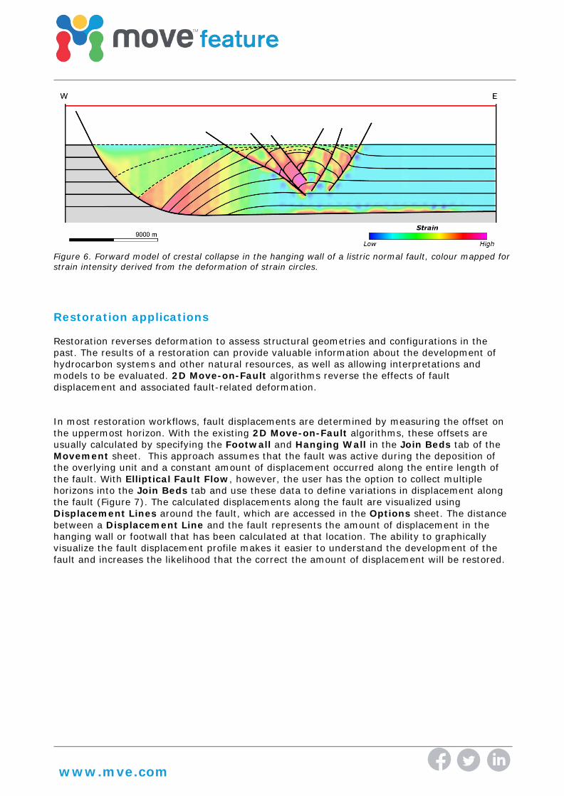
In Move, more complex forward models can be created to better understand the geological evolution of a region. Using the tools within the 2D Kinematic Modelling module, these models can include the effects of multiple faults, syn-tectonic sedimentation, physical compaction, isostasy, post-rift thermal subsidence and salt movement. As an example, a crestal collapse fault system around a hanging wall rollover has been forward modelled using Elliptical Fault Flow (Figure 6). When creating this forward model, strain circle grids for the pre-tectonic and syn-tectonic units were deformed by collecting them as Passive Objects in the 2D Move-on-Fault toolbox. The distribution of strain associated with the development of this crestal collapse fault system was then approximated by measuring the ratio between the long and short axes of the deformed strain circles throughout the section. When the lengths of the long and short axes are similar, the circles have experienced little deformation and the area has a relatively low strain intensity; higher strains result in more distortion of the circles with larger differences between the lengths of the long and short axes.
Figure 6. Forward model of crestal collapse in the hanging wall of a listric normal fault, colour mapped for strain intensity derived from the deformation of strain circles.
Restoration applications Restoration reverses deformation to assess structural geometries and configurations in the past. The results of a restoration can provide valuable information about the development of hydrocarbon systems and other natural resources, as well as allowing interpretations and models to be evaluated. 2D Move-on-Fault algorithms reverse the effects of fault displacement and associated fault-related deformation.
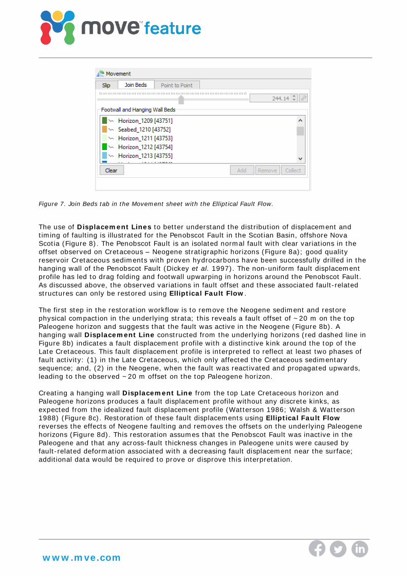
In most restoration workflows, fault displacements are determined by measuring the offset on the uppermost horizon. With the existing 2D Move-on-Fault algorithms, these offsets are usually calculated by specifying the Footwall and Hanging Wall in the Join Beds tab of the Movement sheet. This approach assumes that the fault was active during the deposition of the overlying unit and a constant amount of displacement occurred along the entire length of the fault. With Elliptical Fault Flow, however, the user has the option to collect multiple horizons into the Join Beds tab and use these data to define variations in displacement along the fault (Figure 7). The calculated displacements along the fault are visualized using Displacement Lines around the fault, which are accessed in the Options sheet. The distance between a Displacement Line and the fault represents the amount of displacement in the hanging wall or footwall that has been calculated at that location. The ability to graphically visualize the fault displacement profile makes it easier to understand the development of the fault and increases the likelihood that the correct the amount of displacement will be restored.
Figure 7. Join Beds tab in the Movement sheet with the Elliptical Fault Flow.
The use of Displacement Lines to better understand the distribution of displacement and timing of faulting is illustrated for the Penobscot Fault in the Scotian Basin, offshore Nova Scotia (Figure 8). The Penobscot Fault is an isolated normal fault with clear variations in the offset observed on Cretaceous – Neogene stratigraphic horizons (Figure 8a); good quality reservoir Cretaceous sediments with proven hydrocarbons have been successfully drilled in the hanging wall of the Penobscot Fault (Dickey et al. 1997). The non-uniform fault displacement profile has led to drag folding and footwall upwarping in horizons around the Penobscot Fault. As discussed above, the observed variations in fault offset and these associated fault-related structures can only be restored using Elliptical Fault Flow. The first step in the restoration workflow is to remove the Neogene sediment and restore physical compaction in the underlying strata; this reveals a fault offset of ~20 m on the top Paleogene horizon and suggests that the fault was active in the Neogene (Figure 8b). A hanging wall Displacement Line constructed from the underlying horizons (red dashed line in Figure 8b) indicates a fault displacement profile with a distinctive kink around the top of the Late Cretaceous. This fault displacement profile is interpreted to reflect at least two phases of fault activity: (1) in the Late Cretaceous, which only affected the Cretaceous sedimentary sequence; and, (2) in the Neogene, when the fault was reactivated and propagated upwards, leading to the observed ~20 m offset on the top Paleogene horizon. Creating a hanging wall Displacement Line from the top Late Cretaceous horizon and Paleogene horizons produces a fault displacement profile without any discrete kinks, as expected from the idealized fault displacement profile (Watterson 1986; Walsh & Watterson 1988) (Figure 8c). Restoration of these fault displacements using Elliptical Fault Flow reverses the effects of Neogene faulting and removes the offsets on the underlying Paleogene horizons (Figure 8d). This restoration assumes that the Penobscot Fault was inactive in the Paleogene and that any across-fault thickness changes in Paleogene units were caused by fault-related deformation associated with a decreasing fault displacement near the surface; additional data would be required to prove or disprove this interpretation.
Figure 8. Restoration of a section through the Penobscot Fault, offshore Nova Scotia: (a) Present-day interpretation; (b) Removal of Neogene sediment with the amount of displacement along the fault visualised with red dashed line; (c) Removed Neogene with the amount of displacement along the fault defined by Top Cretaceous and Paleogene horizons visualised with red dashed line; (d) Restoration of Neogene fault slip. Seismic data from Nova Scotia Department of Energy.
From the restored top Paleogene time-step (Figure 9a), the Paleogene units are removed and the associated physical compaction in the underlying strata is restored, revealing the structural configurations at the end of the Late Cretaceous (Figure 9b). This restored time step indicates that the Late Cretaceous sediments are >150 m thicker in the hanging wall of Penobscot Fault than the footwall, confirming that the fault was active in this period. Thicker Late Cretaceous sediments in the hanging wall led to differences in the effects of physical compaction across the fault, resulting in the development of a hanging wall syncline (Skuce 1996); this syncline likely influenced subsequent hydrocarbon migration and could form a possible trap. The removal of the Late Cretaceous sediments and the restoration of the associated physical compaction reduces the amplitude of the hanging wall syncline (Figure 8e). The resulting horizon offsets provide a Displacement Line for the Late Cretaceous phase of fault activity (Figure 9c); the restoration of these fault offsets using Elliptical Fault Flow illustrates the cross section at the top of the Early Cretaceous (Figure 9d). These results suggest that the Early Cretaceous sediments were folded into a broad anticline at this time; this has potential implications for early hydrocarbon migration in the basin.
Figure 9. Continued restoration of a section through the Penobscot Fault, offshore Nova Scotia: (a) Restoration of Neogene fault slip; (b) Removal of Paleogene sediment; (c) Removal of Late Cretaceous sediment with the amount of displacement along the fault visualised with red dashed line; (d) Restoration of Late Cretaceous fault slip. Seismic data from Nova Scotia Department of Energy.
Summary Midland Valley geologists and developers have designed Elliptical Fault Flow to model and restore faults with variable displacements and many of the associated deformational features. The inclusion of this algorithm in Move will allow interpretations of many fault systems to be assessed and validated through kinematic forward modelling for the first time, which in turn, will improve the accuracy of geological models in a variety of settings. Moreover, the relative simplicity of the input parameters for Elliptical Fault Flow, and the ease with which fault displacement profiles can be considered during sequential restoration workflows, will provide a better understanding of subsurface deformation through time.
geometry in the volume containing a single normal fault. AAPG Bulletin, 71 (8), 925-937. Dickey, J., Bigelow, S., Edens, J., Brown, D., Smith, B., Makrides, C. & Mader, R. 1997.
Technical summaries of Scotian Shelf-significant and commercial discoveries. Gibson, J., Walsh, J. & Watterson, J. 1989. Modelling of bed contours and cross-sections
adjacent to planar normal faults. Journal of Structural Geology, 11 (3), 317-328. Nixon, C.W., Sanderson, D.J., Dee, S.J., Bull, J.M., Humphreys, R.J. & Swanson, M.H. 2014.
Fault interactions and reactivation within a normal-fault network at Milne Point, Alaska. AAPG Bulletin, 98 (10), 2081-2107.
Resor, P.G. 2008. Deformation associated with a continental normal fault system, western Grand Canyon, Arizona. Geological Society of America Bulletin, 120 (3-4), 414-430.
Skuce, A. 1996. Forward modelling of compaction above normal faults: an example from the Sirte Basin, Libya. Geological Society, London, Special Publications, 99 (1), 135-146.
Triezenberg, P., Hart, P. & Childs, J. 2016. National Archive of Marine Seismic Surveys (NAMSS): a USGS Data Website of Marine Seismic Reflection Data within the US Exclusive Economic Zone (EEZ): US Geological Survey Data Release (2016) http://dx. doi. org/10.5066, F7930R7P.
Walsh, J.J. & Watterson, J. 1988. Analysis of the relationship between displacements and dimensions of faults. Journal of Structural Geology, 10 (3), 239-247.
Watterson, J. 1986. Fault dimensions, displacements and growth. Pure and Applied Geophysics, 124 (1-2), 365-373.
The authors acknowledge the Bureau of Ocean Energy Management and the US Geological Survey for providing seismic reflection data. Neither the data provider nor the USGS warrant the use of these data, nor make any claims or guarantees as to the accuracy of the data identification, acquisition parameters, processing methods, navigation or database entries. The authors also acknowledge the use of seismic data from the Nova Scotia Department of Energy. If you require any more information about Elliptical Fault Flow or any other 2D Move-on-Fault algorithm in Move, then please contact us by email: [email protected] or call: +44 (0)141 332 2681.