AD-AOO1 614 NAVAL POSTGRADUATE SC1OL MONTEREY CA F/G 12/1 AUTOMATIC FACTORIZATION OF GENERALIZED UPPER BOUNDS IN LARGE SC-f TC(U) JAN 8O 4 6 BROWN, D S THOMEN UNCLASSIFIED NPS55--003 L fllflllllll mllllEEllEEEEI llllllllIENl ElllEEEElllEll -8
Transcript
AD-AOO1 614 NAVAL POSTGRADUATE SC1OL MONTEREY CA F/G 12/1AUTOMATIC FACTORIZATION OF GENERALIZED UPPER BOUNDS IN LARGE SC-f TC(U)JAN 8O 4 6 BROWN, D S THOMEN
UNCLASSIFIED NPS55--003 L
fllflllllllmllllEEllEEEEIllllllllIENl
ElllEEEElllEll -8
S55-80-003NAVAL POSTGRADUATE SCHOOL
Monterey, California
DTIC
A
AUTOMATIC FACTORIZATION OF GENERALIZED
UPPER BOUNDS IN LARGE SCALE
OPTIMIZATION MODELS
by
Gerald G. Brown
and
David S. Thomen
January 1980
" /Approved for public release; distribution unlimited.
U 80
: m I-
NhVAL POSTGRADUATE SCHOOL
WTEREY, CALI FORNIA
Rear Admiral T. F. Dedman Jack R. BorstingSuperintendent Provost
This report was prepared by-
David S. Thomen, CAP"NU .S.- MARINE COR~PS
Reviewed by: Released by:
Michael G. Sovereifgn, Chairn Willia&mM. TollesDepartment Of Operations R~6earch Dean of Research
b.
IF
UNCLASSIFIEDSECURITY CLASSIFICATION OF THIS PAGE ( ten Data Entered)
20. ABSTRACT (Continue on reverse side It necessary and Identify by block number)
To solve contemporary large scale linear, integer and mixed integer pro-gramming problems, it is often necessary to exploit intrinsic specialstructure in the model at hand. One commonly used technique is to identifyand then to exploit in a basis factorization algorithm a generalized upperbound (GUB) structure. This report compares several existing methods foridentifying GUB structure. Computer programs have been written to permitcomparison of computational efficiency. The GUB programs have been _,
OVER
AN I 1473 EDITION OF NOV ISIS OBSOLETE5S/i 0102-014- 601 1
SECURITY CLASSIFICATION OF THIS WAGE (When Data Entered)
UNCLASSIFIED4,;. URTY CLASSIPICATION OF THiS PAGIL(Wbam Date Rnirese
20. ABSTRACT CONT.
incorporated in an existing optimization system of advanced design andhave been tested on a variety of large scale real life-optimizationproblems. The identification of GUB sets of maximum size is shown tobe among the class of NP-complete problems;these problems are widelyconjectured to be intractable in that no polynomial-time algorithm hasbeen demonstrated for solving them. All the methods discussed in thisreport are polynomial-time heuristic algorithms that attempt to find,but do not guarantee, GUB sets of maximum size. Bounds for the maximumsize of GUB sets are developed, in order to evaluate the effectivenessof the heuristic algorithms.
SRCUITY CLASSIFICATION OF THIS PAGK(WhM D. E. 3tW
MMMWMMV_
:' ~~AUTOMATIC FACTORIZATION OF GENERALIZED UPPER BOR a ' : c d
IN LARGE SCALE OPTIMIZATION MODELS
Gerald G. Brown . : e
David S. Thomen L..i, Y./
Naval Postgraduate SchoolMonterey, California
To solve contemporary large scale linear, integer and mixed integer
programming problems, it is often necessary to exploit intrinsic special
structure in the model at hand. One commonly used technique is to identify
and then to exploit in a basis factorization algorithm a generalized upper
bound (GUB) structure. This report compares several existing methods for
identifying GUB structure. Computer programs have been written to permit
comparison of computational efficiency. The GUB programs have been in-
corporated in an existing optimization system of advanced design and have
ibeen tested on a variety of large scale real life optimization problems.The identification of GUB sets of maximum size is shown to be among the
class of NP-complete problems; these problems are widely conjectured to
be intractable in that no polynomial-time algorithm has been demonstrated
for solving them. All the methods discussed in this report are polynomial-
time heuristic algorithms that attempt to find, but do not guarantee, GUB
sets of maximum size. Bounds for the maximum size of GUB sets are developed,
in order to evaluate the effectiveness of the heuristic algorithms.
1. INTRODUCTION
Contemporary mathematical programming models are often so large
that direct solution of the associated linear programming (LP) problems
with the classical simplex method is prohibitively expensive, if not
impossible in a practical sense. It has been found that most of these
problems are sparse, with relatively few non-zero coefficients, and
usually possess very systematic structure. These problems exhibit inherent
structural characteristics that can be exploited by specializations of
the simplex procedure. Various types of regularity are often described
as, for instance, block angular, staircase, and so forth; terms all
chosen to describe the visual appearance of the non-zero ceofficients
when the rows and coluns of the problem are suitably ordered. There
are profound economic, managerial and mathematical motives for this
special structure, which are not examined here.
Methods to exploit special model structure can be categorized
generally as indiea (e.g., decomposition), where a solution to the
original problem is achieved by dealing with related models which are
individually easier to solve, or as d ct, when the original problem is
solved by a modified simplex algorithm.
Among the direct methods, the most frequently used technique is
called bai6 6aeItoLzat.ion (6], where the reflection of special problem
structure appears and is used to good benefit in the intermediate LP
bases. Basis factorization can be dyf&pnt, where the algorithm deals
with each basis sequentially and/or independently in an attempt to extract
as much specialized basis structure as possible, or 4tattc, where the
algorithm depends upon certain types of special structure being
present in WLL bases.2
Static basis factorizations include Ampte uppeA bound6,
geneAotized uppet bound6 (GUB), and embedded ne-&'okk ,U416, among many
others. Simple upper bounds are a set of rows for which each row has
only one non-zero coefficient. Generalized upper bounds are a set of
rows for which each column (restricted to those rows) has at most one
non-zero coefficient. Network rows are a set of rows for which each
column (restricted to those rows) has at most two non-zero coefficients
of opposite sign.
Each of these factorizations permits the simplex algorithm to
deal with the static subsets of the rows (and columns) of all bases
encountered with prior knowledge that they will satisfy veuJ restricted
rules. Most of these methods work best when togic can be substituted
for arithmetic (as is the case with the coefficients + 1). For this
reason, static factorizations often restrict the special structure to
possess only + 1, or to be 4cxaed so as to produce an equivalent result.
The concept of generalized upper bounds was introduced in 1964,
the result of work by Dantzig and Van Slyke [4]. the name is derived
from analogy to the simple upper bound structure. Graves and McBride [61
refer to S~txo Signed Identity Factorzation as a term more suggestive
of the implied basis structure. Since their introduction, some form of
GUB has been implemented in many commercial LP systems. There is often
confusion between the mathematical characterization of GUB and these
various, widely used implementations of GUB, in that the latter often
restrict the GUB set membership rules to permit uncomplicated simplex
logic. All of the methods reported here address the full generality of
GUB sets but can be modified to produce restricted GUB sets as necessary.
3
i_ _ _ . , ,
The details of how GUB can be exploited to reduce the computations
of the simplex algorithm are not discussed here. See [1,4,6,10,12]. The
underlying concept is that the GUB structure enables the simplex algorithm
to manipulate the GUB rows implicitly, with logic rather than floating
point arithmetic, thus reducing the effective size and solution time
for the problem. The more rows one is able to GUB, the fewer rows one
has to explicitly carry through the simplex operations. If the original
problem has m constraints (of which p are GUB rows) and n variables,
then at most only an (m-p x m-p) submatrix of the basis is needed for
the explicit simplex operations. This contracted explicit basis means
that many of the calculations are replaced with logical operations,
yielding faster results and less numerical rounding error.
Many problem types have natural GUB structures embedded in them.
a) "Transportation problems (pure, bounded and capacitated networks)
b) Multi-product blending
c) Raw material and/or production resources allocation (forest management,
To illustrate, Figure 1 presents a transportation type problem.
Note that a GUB set has been marked. For problems similar to this, a
large GUB set can be found quickly by visual inspection. Likewise, in
a particular eLa6 of models, knowledge of the model structure can lead
to problem-independent specification of GUB sets (e.g., one can always
4
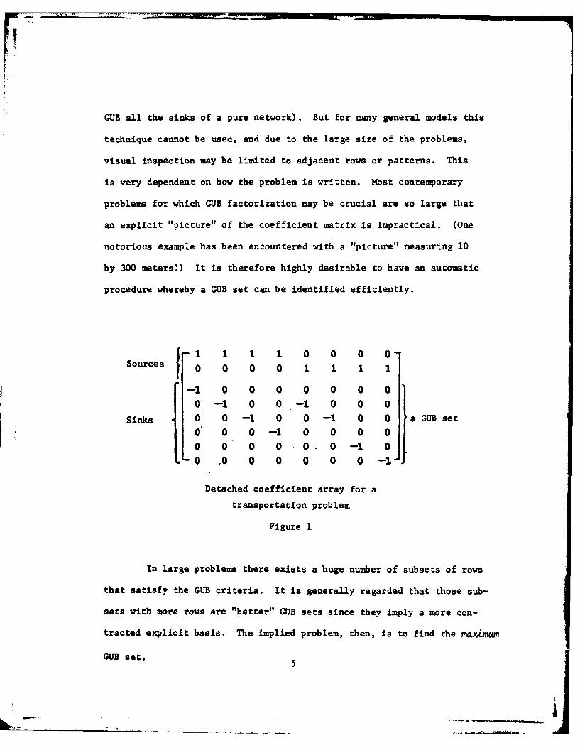
GUB all the sinks of a pure network). But for many general models this
technique cannot be used, and due to the large size of the problems,
visual inspection may be limited to adjacent rows or patterns. This
is very dependent on how the problem is written. Most contemporary
problems for which GUB factorization may be crucial are so large that
an explicit "picture" of the coefficient matrix is impractical. (One
notorious example has been encountered with a "picture" measuring 10
by 300 meters!) It is therefore highly desirable to have an automatic
procedure whereby a GUB set can be identified efficiently.
I 1 1 1 0 0 0 0Sources 0 0 0 0 1 1 1 1
-1 0 0 0 0 0 0 0
0 -1. 0 0 -1 0 0 0
Sinks 0 0 -1 0 0 -1 0 0 a GUB set
0 0 0 -1 0 0 0 0
0 0 0 0 0. 0 -1 0
- 0 .0 0 0 0 0 0 -1
Detached coefficient array for a
transportation problem
Figure 1
In large problems there exists a huge number of subsets of rows
that satisfy the GUB criteria. It is generally regarded that those sub-
sets with more rows are "better" GUB sets since they imply a more con-
tracted explicit basis. The implied problem, then, is to find the max,.um
GUB set. 5
Integer algorithms to find a maximum GUB set do exist.
These usually entail enumeration schemes and cannot be guaranteed to be
efficient in a practical sense. Conceivably, 2m-m sets of rows might
have to be searched before a maximum GUB structure is found. As the
problem size grows, the number of possible sets that need to be checked
increases exponentiaLy. As will be shown later, the hope of finding
an efficient algorithm to find the maXimum GUB set for any general
problem is dim.
Therefore, researchers and practitioners have concentrated on
constructing efficient heuvJ tic algorithms that attempt to identify,
but do not guarantee, a maximum GUB set. A few of these methods show-
ing great promise have been reported, but they have not been tested with
large scale problems.
This report outlines several automatic heuristic GUB finding pro-
cedures that have been developed and published in the recent literature.
These procedures are tested on a suite of large scale, real life optimi-
zation problems, and are modified to improve their behavior. Comparative
performance of the methods is given both in terms of the computational
effort to identify a GUB set, as well as the size of the GUB set
achieved.
Identification of GUB sets of maximum row dimension is shown in
Section 7 to be among the class of NP-complete problems. However, an
easily computed uppet bound on the size of the maximum GUB set is developed
and used to evaluate objectively the quality of heuristic GUB algorithms,
showing that very nearly maximum GUB sets are routinely achieved.
6
2. PROBLEM DEFINITION AND REPRESENTATIONS
The Linear Programning problem is defined as
(L) Minc tx
s.t. r < Ax < r (ranged constraints)
b < x < b (simple bounds)
where r and r are m-vectors, x, c, b and b are n-vectors and A
is an m x n matrix. The constraints are sometimes defined as equations,
but for the general case of GUB treated here constraints can be equations,
inequalities or a mixture. The immediate discussion will be directed
at (L); integer and mixed integer problems are treated later.
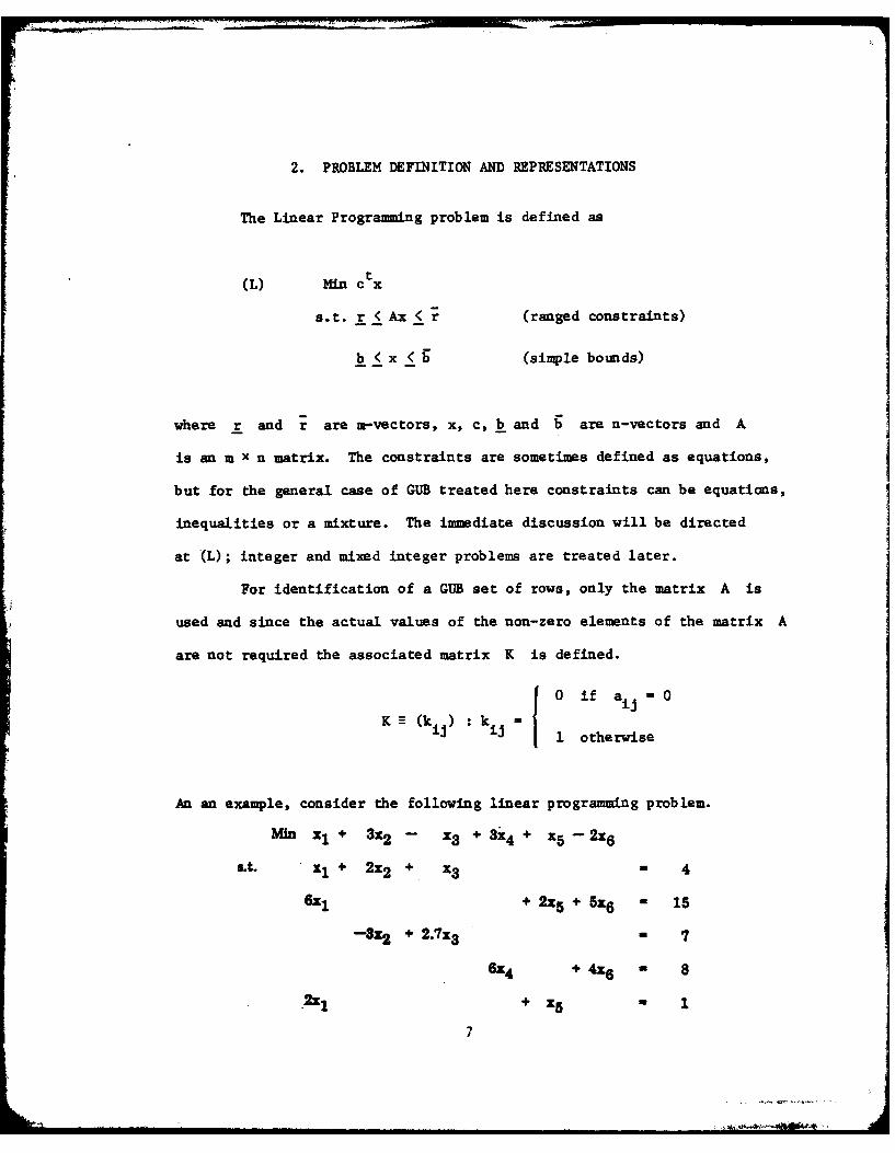
For identification of a GUB set of rows, only the matrix A is
used and since the actual values of the non-zero elements of the matrix A
are not required the associated matrix K is defined.
0 if a 0
K- (ki ) : kiij ki i 1 otherwise
An an example, consider the following linear programming problem.
Min x, + 3x2 - x3 + 3i 4 + x5 -2x 6
s.t. x 1 + 2x 2 + x3 4
6x I + 2X5 + 5z 6 15
-3x 2 + 2.7x 3 7
6Z4 + 4U6 = 8
.2 +s x+ 1
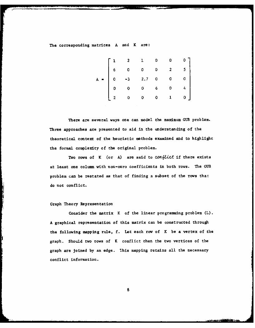
The corresponding matrices A and K are:
1 2 1 0 0 0
6 0 0 0 2 5
A 0 -3 2.7 0 0 0
0 0 0 6 0 4
2 0 0 0 1 0
There are several ways one can model the maximum GUB problem.
Three approaches are presented to aid in the understanding of the
theoretical context of the heuristic methods examined and to highlight
the formal complexity of the original problem.
Two rows of K (or A) are said to con 6ct if there exists
at least one column with non-zero coefficients in both rows. The GUB
problem can be restated as that of finding a subset of the rows that
do not conflict.
Graph Theory Representation
Consider the matrix K of the linear programming problem (L).
A graphical representation of this matrix can be constructed through
the following mapping rule, f. Let each row of K be a vertex of the
graph. Should two rows of K conflict then the two vertices of the
graph are joined by an edge. Ihis mapping retains all the necessary
conflict information.
8
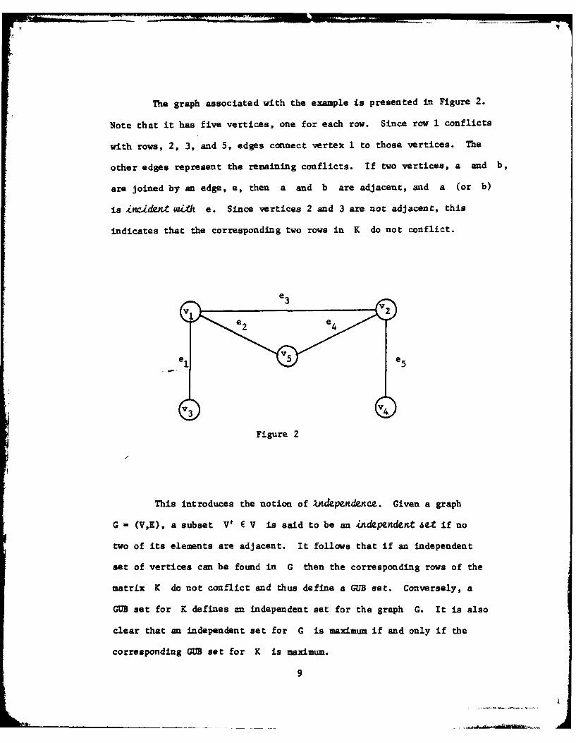
The graph associated with the example is presented in Figure 2.
Note that it has five vertices, one for each row. Since row 1 conflicts
with rows, 2, 3, and 5, edges connect vertex 1 to those vertices. The
other edges represent the remaining conflicts. If two vertices, a and b,
are joined by an edge, e, then a and b are adjacent, and a (or b)
is incident with e. Since vertices 2 and 3 are not adjacent, this
indicates that the corresponding two rows in K do not conflict.
e 3
e 2 e 4
e v5 e5
Figure 2
This introduces the notion of ndependnce. Given a graph
G - (V,E), a subset V' E V is said to be an independent 6et if no
two of its elements are adjacent. It follows that if an independent
set of vertices can be found in G then the corresponding rows of the
matrix K do not conflict and thus define a GUB set. Conversely, a
GUB set for K defines an independent set for the graph G. It is also
clear that an independent set for G is maximum if and only if the
corresponding GlB set for K is maximum.
9
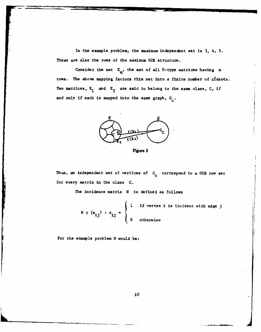
In the example problem, the maximum independent set is 3, 4, 5.
These are also the rows of the maximum GUB structure.
Consider the set Kin, the set of all K-type matrices having m
rows. The above mapping factors this set into a finite number of ct46AeA.
Two matrices, K1 and K2 are said to belong to the same class, C, if
and only if each is mapped into the same graph, Gc.
K
G
Thus, an independent set of vertices of G correspond to a GUB row setc
for every matrix in the class C.
The incidence matrix N is defined as follows
I1 if vertex i is incident with edge j
N0 otherwise
For the example problem N would be:
10
61 e2 e3 64 e5
v1 1 1 1 0 0
v2 0 0 1 1 1
N - v3 1 0 0 0 0
T4 0 0 0 0 1
v5 0 1 0 1 0
There exists one, and only one incidence matrix for each graph of G,
where G is the set of all graphs having m vertices.
Since the set of all N-type matrices with m rows is a subset
of Kin, every class of K contains one and only one incidence matrix.
In general, for the GUB problem, every m row matrix is equivalent
to one of a finite number of incidence matrices. Superficially this
may seem to be a simplfication. But as shown in Section 7 the GUB
problem on N is as difficult as the independent set problem on G.
The equivalent statements of the GUB problem do, however, offer
different views of the problem which are helpful in considering algorithms
for and analysis of the problem. [Note: In Garey and Johnson (51 it
is shown that two other graph problems, the "vertex cover" and the "clique"
problem, are equivalent to the independence problem, and hence the GUB
problem. These problems do not seem to offer any additional insight
for the GUB problem. ]
Conflict Matrix Representation
The first heuristic approach is developed around a conitict matAix.
This is a square matrix of dimension m, defined by:
11
1 if row i conflicts with row j in (L)
M (Mjj) i0 otherwise.
For the example problem:
1 1 1 0 11 1 0 1 1
M- 1 0 1 0 0 .
0 1 0. 1 0
1 1 0 0 1
Note that this matrix is symmetric. The sum for any row (or column)
indicates the number of other rows it is in conflict with, plus one.
This sum is important in that it indicates for any particular
row how many other rows would be subsequently excluded from a GUB set
by its addition.
The rows of a GUB structure can be rearranged to form an
embedded identity matrix in M. Note that this is the case for rows
3, 4, and 5 in the example problem.
Vector Space Representation
The second heuristic approach can be modeled using vectors in
an n-dimensional vector space, where n is the number of variables in
the problem (L). Consider each row of K as a vector in this space,
having unit length in those "dimensions" corresponding with its non-zero
coefficients. In the example problem, row 1 is represented by the
following vector:
12
(1,1,i,0,0,0)•
R, the resultant vector from the sum of all vectors of the rows
of K, indicates the number of conflicts, plus one, associated with each
variable of (L). A hypercube in n-space situated in the first orthant
at the origin with length 1 in all positive directions denotes the
feasible GUB region. Should R extend beyond this aree, then the set
of rows corresponding to the vectors determining R does not constitute
a GUB structure.
A gradient vector can be calculated indicating the direction of
the shortest distance to the 6euibte xegion. It can be used to determine
which row to remove from the set to obtain the largest movement on the
desired direction. When R falls within the feasible region, the set
of rows determining R constitutes a GUB set.
13
3. EARLIER LITERATURE
Two papers dealing with efficient GUB finding methods are worthy
of special note.
Brearley, Mitra and Williams (2] establish a very useful framework
for study of methods for finding GUB structure, as well as an insightful
discussion of these methods and a taxonomy for their classification.
They define three sets consisting of the rows of the technological
matrix A. The first set, the e-Ugibe 2et, is made up of every row of
A that is individually eligible to belong in the GUB set. The 6t'uCxtuA
6et is a subset of the eligible set and includes all those rows currently
considered as members of the GUB set. The candidate 4et consists of
those rows of the eligible set that are candidates for inclusion (or re-
inclusion) in the GUB set. Every one of the methods examined in [2]
is described in terms of manipulation of these sets.
Each method of building a GUB set employs one of two basic strategies
1he type I (row additio0n) strategy begins with an empty structure set.
Then, based on a particular type I criteria for inclusion, rows are removed
from the candidate set and either added to the structure set or dropped
from further consideration. This procedure continues until the candidate
set is empty. The rows in the structure set form an admissible GUB
structure.
The type I (row deletion) strategy takes the opposite approach and
is divided into two phases. Methods of this type initially place all
eligible rows in the structure set. This normally leads to an infeasible
GUB set with many conflicting rows. Based upon the particular type II
14
decision rules, rows are removed from the structure set and placed in
the candidate set. The first phase of this strategy ends when a feasible
structure is obtained.
The second phase involves examining the removed rows in the
candidate set. Those that do not conflict with any of the members of
the current structure set are taken from the candidate set and reincluded
in the structure set. Those that do conflict are deleted from the can-
didate set and dropped from further consideration. The second phase ends
when the candidate set is empty. At this point the rows of the structure
set constitute an admissible GUB set.
Brearley, Mitra, and Williams examine over 18 different methods.
These approaches differ in the primary and secondary decision criteria
for including (or removing) a row in the GUB structure set. The heuristic
decision rules examined are based on the following model entities and
combinations thereof:
Include or remove a row based upon:
a) the number of non-zero elements in the given row,
b) the number cf rows in conflict with the given row,
c) the number of non-zero elements in rows that conflict with the given row,
d) the row's relative weight obtained by the inner product of a vector
representation of the row and a directional gradient.
Type I methods, using all these rules were tested, as were Type II
methods using rules a, b and c. As an example, 1.1 (type I strategy,
method number 1) has as its primary decision rule for adding rows to the
structure set: choose a row from the candidate set with the minimum
number of non-zero elements. Method II.1 removes rows from the structure
set based upon the maximum non-zero element count for each row.
15
These methods were implemented with an ALGOL program run on
an ICL 4130 computer. Twelve linear programming problems ranging in
size from 12 rows up to 166 rows were used for computational tests.
The results show that those (Type I) methods using heuristic (d)
above "consistently performed very well" (2]. Similarly, those methods
using heuristic (b) were found to perform nearly as well as (d).
McBride [15] compares the directional gradient method (d) with
an approach suggested, but not tested by Greenberg and Rarick [7]. The
latter method uses the conflict matrix as does heuristic (b). However, it
focuses on finding a maximum embedded identity matrix within the conflict
matrix, rather than using the conflict matrix to determine conflict
counts, applying a specialization of the preassigned pivot procedure (P 3)
normally used for reinversion [8]. McBride's results indicate that
heuristic (d) is significantly faster. However, neither method consistently
achieves a larger GUB set.
McBride also comments on the notion of a "good" GUB set. He
finds merit in selecting a set of GUB rows that minimizes the non-zero
build-up in the representation of the inverse transformation of the explicit
basis, during actual optimization. Results are also given for a restricted
GUB set selection that gives priority to equality constraints. Since
equality constraints are always binding in feasible solutions, the subset
of the basis associated with binding constraints, or kernel [6] is expected
to have fewer explicit non-zero elements.
Based upon the results in these papers, and on independent com-
putational experience with automatic GUB factorization reported by Brown
16
and Graves [3], the present research initially concentrated on those
approaches utilizing the two most successful heuristics, based on
conflict (1.2, 11.2) and directional gradient (11.9, 11.10).
The models studied in this report are of a larger scale and include
mixed integer problems as well as models for which prior GUB row sets
have been manually specified.
Most of the notation and labels of (2] have been retained here.
17
4. DETERMINATION OF THE ELIGIBLE SET
The implementation of GUB in simplex algorithms usually admits
only + 1 as non-zero coefficients in the GUB rows. In linear programming,
a column scaling can make each non-zero element in a GUB row + 1. For
variables of an integer or mixed integer programming problem, the columns
of matrix A that correspond to integer variables cannot be scaled without
inconvenience for other optimization functions depending upon the integrality
condition. Therefore, non-zero elements in columns corresponding to
integer variables will be modified only by row scaling. If it is impossible
to obtain the necessary + 1 non-zero coefficients by row scaling and
column scaling of columns corresponding to continuous-valued variables,
the row is deemed not eligible for inclusion in a GUB set.
It is an objective of this research that the procedures examined
for locating a GUB set in a linear programming problem be designed to be
incorporated as an automatic, integral part of a contemporary optimizing
system of advanced design.
Each method is implemented as a feature of the read routine
(written to accept input in the standard MPS format, as well as editing
information indicating integer variables, scaling, andknown prior GUB
structure). Each method automatically examines the rows of the input
and specifies a GUB set. The appropriate rows and columns are then
scaled as necessary to obtain the proper GUB structure, and passed on to
the optimizing portion of the system. (Note that the editing information
places conditions that must be satisfied for any achievable GUB set.)
18
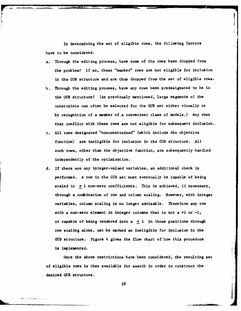
In determining the set of eligible rows, the following factors
have to be considered.
a. Through the editing process, have some of the rows been dropped from
the problem? If so, these "masked" rows are not eligible for inclusion
in the GUB structure and are thus dropped from the set of eligible rows.
b. Through the editing process, have any rows been predesignated to be in
the GUB structure? (As previously mentioned, large segments of the
constraints can often be selected for the GUB set either visually or
by recognition of a member of a convenient class of models.) Any rows
that conflict with these rows are not eligible for subsequent inclusion.
c. All rows designated "nonconstrained" (which include the objective
function) are ineligible for inclusion in the GUB structure. All
such rows, other than the objective function, are subsequently handled
independently of the optimization.
d. If there are any integer-valued variables, an additional check is
performed. A row in the GUB set must eventually be capable of being
scaled to + I non-zero coefficients. This is achieved, if necessary,
through a combination of row and column scaling. However, with integer
variables, column scaling is no longer advisable. Therefore any row
with a non-zero element in integer columns that is not a +1 or -1,
or capable of being rendered into a + 1 in those positions through
row scaling alone, ust be marked as ineligible for inclusion in the
GUB structure. Figure 4 gives the flow chart of how this procedure
is implemented.
Once the above restrictions have been considered, the resulting set
of eligible rows is then available for search in order to construct the
desired GUB structure.
19
Zurga T
C=1a
I M~xI
91s"4
i0
DOkfrc m
5. IMPLEMENTATION OF AUTOMATIC GUB HEURISTICS
Conflict Methods
The approaches 1.2 and 11.2 employ the notion of a conflict measure
for each row. Consider the conflict matrix, M, of the corresponding
technological matrix A, for which a GUB set is to be found. An individual
element, maik is 1 if row i and row k of the original matrix have at
least one column j such that a j 0 0 and akj 0 0. If the two rows
have no non-zero coefficients in a common column then the corresponding
mik of the conflict matrix is 0. Summing across a row of the conflict
matrix can thus give the measure of the number of rows plus one that are
in conflict with a given row. For a given row, this sum less one indicates
exactly how many other rows would be immediately excluded from the GUB
set by incluslion of this row, called the row's detion potenZal.
Method 1.2 initially places all the eligible rows on a candidate
list. From the candiate list, individual rows are selected and removed
to be added to the structure set. Other rows that are in conflict with
the selected row are immediately removed from the candidate list and dis---
carded.
The heuristic selects those rows on the candidate list with the
minimum deletion potential to be added to the structure set first. The
selection of rows for the structure set and the discarding of conflicting
rows continues until the candidate l13t is exhausted. The resulting
structure set forms a GUB set.
A modification' to the above heuristic is possible which bueak tie4
among rows sharing the minimum deletion potential by selecting the row
having the most non-zero elements for inclusion into the GUB structure set.
21
The program used to test this heuristic approach is adapted from an
earlier version made available by Graves. A step by step description of the
method is given below.
Step 1. Identify Eligible Rows. Set B. 1 if row i is an eligible row,
and equal to 0 otherwise.
Step 2. Determine Deletion Potential. Scan each eligible row i and incre-
ment i by the number of other eligible rows k where aij and ak are
both non-zero for at least one column J. (Bi is the deletion potention,
plus one.)
Step 3. Stopping Condition. If all the - 0, stop. Otherwise, go to
the next step.
Step 4. Row Selection. Select row i having the minimum positive ("deletion
potential") si and add it to the structure set.
Step 5. Exclude Rows in Conflict with Selected Row. Locate the (s i- 1 ) rows
in conflict with the selected row i. For each of these rows k, locate the
($k-l) rows that they are in conflict with and decrement S, for those
rows by one.
Step 6. Marking Selected and Excluded Rows Ineligible for Further
Consideration. Set s i and the Bk's equal to zero. Go to step 3.
Only rows with i > 0 are eligible. In step 1, $i is set to 1 for eligible
rows. In the next step the B's for these rows are modified by each row's
deletion potential. Assuming there are still some eligible rows, the one
with the smallest deletion potential is selected in step 4
22
for inclusion in the structure set. In the next step all the rows con-
flicting with the one selected are identified for discard and the deletion
potentials of the remaining rows are updated. In the last step, both the
selected row's weight and those of the discarded rows are set equal to
zero. When all rows have either been selected or discarded the B array
will be all O's. At this point the selected rows from a GUB structure.
Methud 11.2 (row deletion) initially places all the eligible rows
in the structure set. From this set individual rows are selected and
placed on the candidate list in order of maximum deletion potential.
During Phase 2, Brearley, Mitra, and Williams drop all rows from further
consideration that conflict with the structure set and attempt to reinclude
remaining candidate rows (that do not conflict with the structure set) in
LOFI order. A modification of phase 2 is used in this research which
simply excludes from further consideration all conflicting rows, reincludes
any remaining candidate rows, and repeats phase 1, until no further non-
conflicting candidates remain.
Gradient Methods
The second method (II.9, II.10) employs a heuristic method put
forth by Senju and Toyoda [17] for approximate solution of certain linear
programming problems with 0, 1 variables. The general problem they address
is that of choosing a most profitable combination (or portfolio) of orders
subject to resource constraints and an all-or-nothing (0-1) restriction
on the orders (i.e., an order is not allowed to be only partially filled).
This same format can be used to express the search for a maximum
GUB structure in (L). The rows of the technological matrix A are treated
23
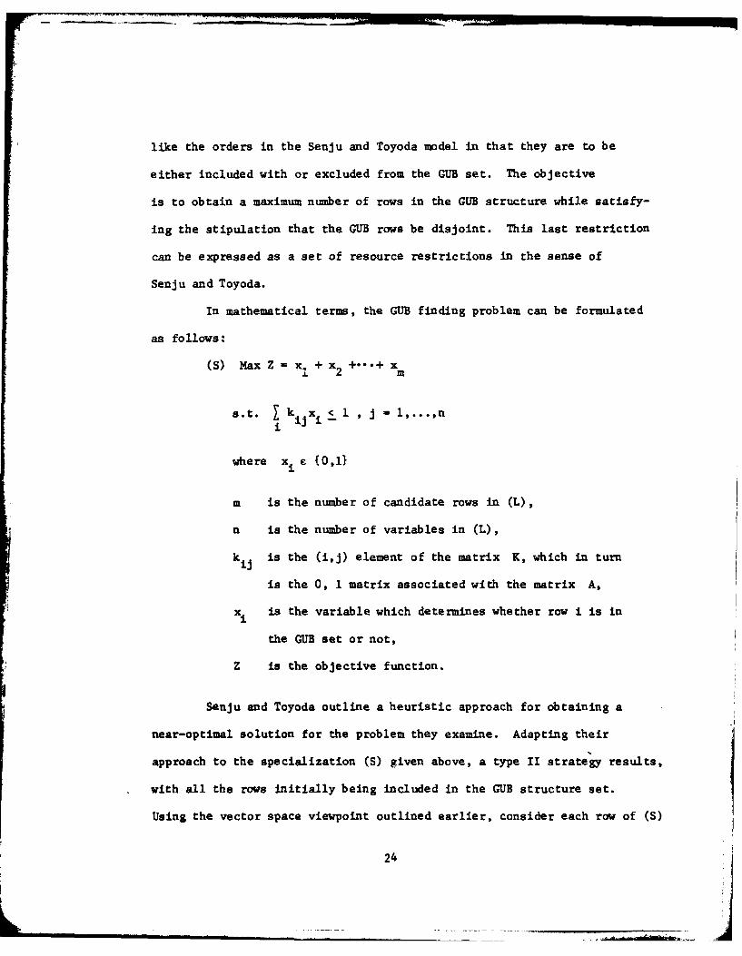
like the orders in the Senju and Toyoda model in that they are to be
either included with or excluded from the GUB set. The objective
is to obtain a maximum number of rows in the GUB structure while satisfy-
ing the stipulation that the GUB rows be disjoint. This last restriction
can be expressed as a set of resource restrictions in the sense of
Senju and Toyoda.
In mathematical terms, the GUB finding problem can be formulated
as follows:
(S) Max Z x, + x2 +--.+ xm
s.t. [ k x < 1i j - 1.. .,ni iii- "
where xi C {0,i}
m is the number of candidate rows in (L),
n is the number of variables in (L),
kij is the (i,j) element of the matrix K, which in turn
is the 0, 1 matrix associated with the matrix A,
xi is the variable which determines whether row i is in
the GUB set or not,
Z is the objective function.
Senju and Toyoda outline a heuristic approach for obtaining a
near-optimal solution for the problem they examine. Adapting their
approach to the specialization (S) given above, a type II strategy results,
with all the rows initially being included in the CUB structure set.
Using the vector space viewpoint outlined earlier, consider each row of (S)
24
as a vector in n-space. A resultant vector R is determined by the
sum of all the included rows and, in general, extends beyond the feasible
space denoted by the unit hypercube. A gradient vector is calculated
from this infeasible point in the direction of the shortest distance to
the feasible region. In Brearley, Mitra and Williams [2] this vector
IIis labeled a . An inner product of this gradient with each of the
row vectors results in a relative weight for each row. These weights,II
which are stored in a vector labeled v can be viewed as indicating
the relative contribution that the removal of the corresponding row
would have towards obtaining a feasible structure set.
Rows are removed from the structure set according to their
relative weight, the largest weight being removed first. This process
is continued until a feasible set of GUB rows has been obtained. (The
gradient vector is not recomputed as the method proceeds.)
Next, a phase 2 procedure is implemented which examines each of
the initially removed rows to see if any can be reincluded into the
structure set without violating the bounds of the unit hypercube. Upon
completion of phase 2, the selected rows constitute a GUB set.
A variation on the above procedure recalculates the shortest
distance to the feasible region after the removal of each row. With the
new gradient, a new set of relative weights for the remaining rows is
then calculated and used, if necessary, to determine which of the subsequent
rows will be removed. This method is named 11.9.
Another modification is possible if two rows are found with equal
weights. As a tie-breaking rule, the row found to have the least number
of non-zero coefficients is discarded first.
25
A step by step outline of the heuristic approach II.10 follows:
Phase 1: Deletion of Infeasible Rows
Step 0. Initialize Sets. Add all eligible rows to the structure
set. The candidate set is empty.
Step 1. Determine the Vector R. For each column J, define p as
the number of rows in the structure set having non-zero elements
in column J.
Step 2. Determine Relative Weight of each Row. For each row i,
define vi as the sum of (P j-l) of every column J, for which a ij 0.
Step 3. Feasibility Condition. If for every column, pj c 1, then go
to step 6; else find a column j such that p > 1.
Step 4. Determine Row for Exclusion. Examine the rows in the
structure having non-zero elements in column J. Select the row i
with the largest v i -
Step 5. Remove Selected Row. Remove row i from the structure set,
decrementing p by one for every column j with a # 0. Add row i
to the candidate set and return to step 3.
Phase 2: Improve Feasible GUB Set Found by Re-including Excluded Rows
Step 6. Eliminate Rows in Candidate Set that Conflict with the Feasible Set.
For every row i of the candidate set that has at least one a # 0ij
in a column with p - 1, remove that row from the candidate set.
Step 7. Re-inclusion of Rows. If any rows remain in the candidate
set, then find row i having the smallest vi . Remove row i from the
candidate set and re-include it in the structure set. Increment Pj
by one for every column j where aij # 0.
Step 8. Stopping Condition. If the candidate set is empty, stop;
else go to step 6.26
In Step 1, the vector P is calculated as the col- counts of non-
zero coefficients. Step 2 calculates the relative weights that result from
the inner product of the gradient vector with each of the row vectors.
These are stored in the array v. The next step examines p to see if the
vector is within the feasible region. If not, a row with the largest relative
weight is removed from the structure set and the p vector is updated to
reflect the sum of the row vectors remaining in the structure set.
Once a feasible structure has been obtained, the candidate set (which
consists of those rows initially removed) is scanned in Step 6. Any of those
rows found to still be in conflict with the rows of the structure set are
discarded. Among those rows which remain, that with the smallest relative
weight is re-included in the structure. This cycle of discarding and re-
inclusion is continued until the candidate set has been emptied. The result-
ing rows of the structure set constitute a feasible GUB set.
To modify the algorithm in order to compute a new gradient vector
after the removal of each row in phase 1, step 5 is changed as follows (11.9):
Step 5.* Remove Selected Row. Remove row i from the structure,
decrementing p by one for every column j such that a # 0. Locate
each row k that is in conflict with row i. Decrement v k by the
number of conflicts between the two rows. Add row i to the candidate
set and return to step 3.
Now when a row is removed from the structure set, the v i contain
the new relative weights equal to the inner product between the vector for
row i and the neW gradient.
27
These two basic methods have been implemented as integral modules
of a large scale optimization system. Therefore, explicit conflict matrices
are not built. (To have done so would have consumed too much computer
time and space.) Instead, all the information is stored in the vectors 0,
p, and v. Logical flags associated with each row indicate whether it is
eligible, and whether it is in the candidate set or in the structure set.
As mentioned previously, the problem data is read in MPS format and
expressed internally in terms of only the non-zero elements. This input is
stored in a doubly linked list having both a row and a column thread. Thus,
along with any non-zero coefficient aij, the location of adjacent non-zero
elements in both the row i and column J are also inediately available. This
crucial feature permits efficient row access for various operations (e.g.,
to locate all rows that conflict with a given row at a particular column).
28
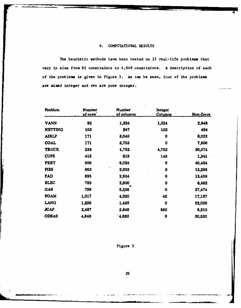
6. COMPUTATIONAL RESULTS
The heuristic methods have been tested on 15 real-life problems that
vary in size from 92 constraints to 4,648 constraints. A description of each
of the proble-m is given in Figure 5. As can be seen, four of the problems
are mixed integer and two are pure integer.
Problem Number Number Integerof rows" of columns Columns Non-Zeros
VANN 92 1,324 1,324 2,648
NETTING 103 247 103 494
AIRLP 171 3,040 0 6,023
COAL 171 3,753 0 7,506
TRUCK 239 4,752 4,752 30,074
CUPS 415 619 145 1,341
FERT 606 9,024 0 40,484
PIES 663 2,923 0 13,288
PAD 695 2,934 0 13,459
ELEC 785 2,800 0 8,462
GAS 799 5,536 0 27,474
FOAM 1,017 4,020 42 17,187
LANG 1,236 1,425 0 22,028
JCAP 2,487 3,849 560 9,510
ODSAS 4,648 4,683 0 30,520
Figure 5
29
... .. ..1f - --,,,.-- .-
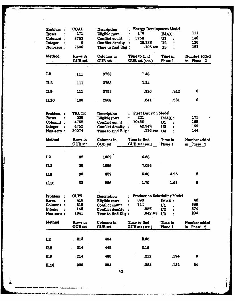
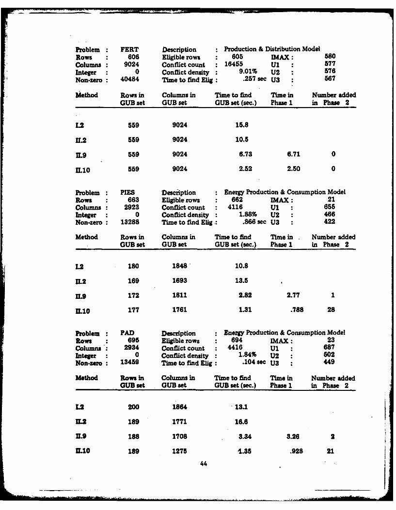
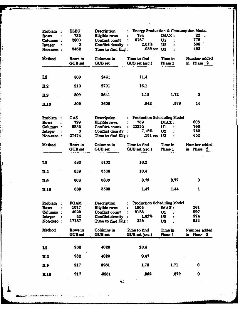
The results of these experiments are given in Appendix A. The first
two columns give the rows and non-zero column elements, respectively, of the
GUB structures found. The time given in column three is the time required to
locate the GUB set once the set of eligible rows has been determined. The
final columns give additional information relating to the two versions of
the gradient methods examined and represents total time in phase 1 and the
number of rows re-included in the GUB structure during phase 2. All
execution times reported are expressed in actual CPU seconds, accurate to the
precision displayed, for IBM 360/67 and FORTRAN H (Extended).
As with the earlier work cited, the Senju and Toyoda method was found
to be consistently the fastest. In general this holds true for both method
II.9 and II.1O. 11.9, which updates the gradient after each row is removed,
takes longer in phase 1 than its counterpart. However, it so selectively
deletes the rows, that few if any rows are ever added back into the structure
during phase 2. This suggests the possibility of implementing 11.9 as
only a one phase method.
All methods are robust in chat they consistently find large GUB sets.
The conflict approaches generally find a larger number of variables with
non-zero coefficients in the CUB rows. However, this approach definitely
becomes inefficient when larger problems are analyzed, regardless of the
relative size of the GUB structure in the problem.
There is some discrepancy between these results and those published
earlier (21, especially with regard to the times of the other methods com-
pared to 11.10. The wide discrepancy between II.9 and II.10 has not been
observed in the current experiments. It is hypothesized that this is due
partially to differences in implementation of the various approaches and
partially to problem size and structure variations between these studies.
30
7. PROBLEM COMPLEXITY
The Compeez of a problem is said to be polynomial if an algorithm
exists for which the fundamental operations are limited by a polynomial func-
tion of intrinsic problem dimensions. Such an algorithm would be called a
potynomia time or good algorithm. The class of all problems for which such
algorithms exist is denoted (P). If an algorithm is not polynomial time,
then it is defined to be an exponentlaP tim algorithm. The disadvantage
of an exponential algorithm is the explosive growth of the maximum solution
time as the dimensions of the problem increase [13].
A problem x is said to be dLibte to a problem y if each good
algorithm for solving y can be used to produce in polynomial time a good
algorithm for solving x [11]. Note that this does not necessarily require
that a good algorithm for x and y actually exist. This requires only
that if one exists for y, then one also exists for x.
An inbt'ctabe problem is one for which it is known that no polynomial
time algorithm exists. In between this class of problem, and the class P,
is a vast number of problems whose status is uncertain. Among these is a
class of nOteum~ni~t.r-. potynomit -ti n problems (NP) for which a poly-
nomial time algorithm can be shown to exist that can ve y a guessed solu-
tion, but for which the existence of a (deterministic) polynomial time
algorithm to actually solve a problem has not yet been demonstrated.
If every problem of the class NP is reducible to the problem y,
then y is said to be NP-ho Ad. In addition, if y itself belongs to NP,
then y is NP-Compete (5,11].
31
The following problem is known as the independent 6et dec,-ion pubtbem
(ISD). It belongs to the set of NP-complete problems.
(ISD) Given a graph G - (V,E) and an integer t, decide whether G con-
tains an independent set of size t or more.
The GUB decision problem (GUBD) can be defined as follows:
(GUBD) Given an m x n 0,1 matrix K and an integer p, decide whether K
contains a set of p or more rows il, 12, ... , i such thatq
, ej <1 for every column; q > p.e-l e
Given an instance of the ISD problem, the incidence matrix N can be con-
structed. This matrix along with the integer t is an instance of the GUBD
problem. The following theorem proves the correctness of this reduction:
Theorem: The incidence matrix N has t rows satisfying (*) if and only
if there are t vertices in G that are independent.
Proof.
a) Assume there exists t rows of N that satisfy (*). They correspond
to vertices vilvi, ... , v t in G. If any two of these vertices
are adjacent, then
t n 2el l e
where j is the colun in N that corresponds to the edge connecting
the two vertices. This is a violation of the assumption, hence the
t vertices in G are not connected to one another.
32
b. Assume there exists t vertices v , ... ,v in G that are1 2 t
independent. Since no two are adjacent, the corresponding rows in N
satisfy (*) [201. Q.E.D.
Since the ISD problem, a problem known to be NP-complete, is reducible
to the GUBD problem, it follows that the GUBD problem itself is NP-complete.
(It is clear that the reduction is polynomial time and it is also clear that
GUBD is in NP.) The related problems of finding a maximum independent set
and a maximum GUB set are not in NP, however, they are NP-hard. It is there-
fore unlikely that a polynomial-time algorithm will be found for these
problems. Only exponential-time algorithms are presently available.
The above analysis of GUB algorithms has only addressed the mOut Caae
bound. No conclusions are made about the average performance of an algorithm.
In other words, the possibility of the existence of an algorithm with good
average performance, but having an exponential worst case bound, has not
been ruled out.
33
8. AN UPPER BOUND FOR THE SIZE OF MAXIMUM GUB SET
The intrinsic difficulty of identifying a maximum GUB set has been
shown to be exponential, making this task essentially impossible for problems
of the scale at hand. However, the efficient heuristic procedures have been
shown to provide very large GUB sets, whose size appears to be relatively
stable for each problem regardless of the particular method applied. This
suggests that these large GUB sets may be, in fact, very nearly maximum,
although there is no practical way to verify this directly.
Although the problem of determining the size of the maximum GUB set
is also NP-hard, it is possible to develop an easily computable uppe bound on
the maximum GUB set size. This bound can then be used to objectively
evaluate the quality of the GUB sets produced by heuristic algorithms.
It is clear that the number of rows of a GUB set can be no greater
than the number of rows in the problem. Also any one row by itself can form
a GUB set. But these bounds are of little practical use where considering
the problem of identifying a maximum GUB set. Utilizing information that
is already available in the heuristic procedure, it is possible to construct
in polynomial time an upper bound on the size of the maximum GUB set. (It
is also possible to construct a lower bound on the size of the maximum GUB
set, but that topic is not pursued in this report.)
For the purpose of developing a better bound, the incidence matrix
representation (N) of the problem is used. Let si be the number of l's
in row i. Note that s is the number of edges incident to vertex i in G.
Also note that si - 1i-l. The number of columns in N represents the
number of distinct conflicts that exist between the rows of the original
problem. This number is denoted as c, and can be found by the following
formula.34
- -.-~*.
m1i
i-i2
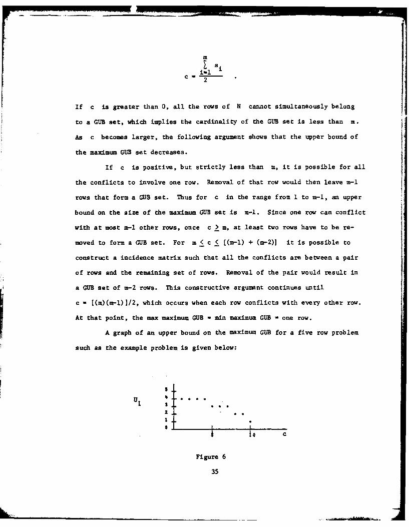
If c is greater than 0, all the rows of N cannot simultaneously belong
to a GUB set, which implies the cardinality of the GUB set is less than m.
As c becomes larger, the following argument shows that the upper bound of
the maximum GUB set decreases.
If c is positive, but strictly less than m, it is possible for all
the conflicts to involve one row. Removal of that row would then leave m-l
rows that form a GUB set. Thus for c in the range from 1 to m-1, an upper
bound on the size of the maximum GUB set is m-1. Since one row can conflict
with at most m-I other rows, once c > m, at least two rows have to be re-
moved to form a GUB set. For m < c < ((m-l) + (m-2)] it is possible to
construct a incidence matrix such that all the conflicts are between a pair
of rows and the remaining set of rows. Removal of the pair would result in
a GUB set of m-2 rows. This constructive argument continues until
c - [(m)(m-1)1/2, which occurs when each row conflicts with every other row.
At that point, the max maximum GUB - min maximum GUB - one row.
A graph of an upper bound on the maximum GUB for a five row problem
such as the example problem is given below:
U ..
210 0
c
Figure 6
35
For the example problem, m - 5 and c - 5. From the above graph the upper
bound on the maximum GUB for that problem is 3. Since a GUB set containing
three rows has already been identified, that set is a maximum set.
In general, for any problem with an m x c incidence matrix, the
largest maximum GUB set that can be obtained is:
U L.5 + /.25 + (m)(m-1) - 2c
where L indicates truncation to an integer.
The above bound is probtem--independent and a Aha.Wp bound in that
matrices with a GUB set the size of the bounding value can be constructed.
With additional information about a specific problem a better bound
can be constructed. Since s i is the number of other rows that conflict
with row i, removing row i from the set of rows reduces the number of con-
flicts, c, by s i . Let IMAX denote max s . Since IMAX is the largest
row conflict count, c can be reduced by no more than IMAX with the removal
of each row. The minimum number of rows that would have to be removed to
reduce the number of row conflicts to 0, is [c/IMAX. Therefore, given m,
c and IMAX, the bound can be improved to
m - , c < (m-y)yyu 2
.5 + .25 + y(2m-y-l) - 2c c > (m-y)(y)
where y - IMAX and r indicates the next higher integer.
In order to determine IMAX, the entire 8 vector must be examined.
A third, even better bound can be obtained with additional information
on the S4zque £y of the conflict counts from 1 to IMAX. The procedure is
the same as above, in that when a row is removed with IMAX conflict count,
36
c decreases by IMAX. However, instead of continuing to decrease c by
IMAX, it is decreased by the next largest s . This procedure continues
until once again, c becomes zero. This bound is named 3"
Each tighter bound requires more information about the particular
problem. However, all the information is readily available since it is
generated by the heuristics using the conflict measure.
The bounds developed can be used to objectively evaluate the size
of a GUB set found by heuristic methods. In two problems examined, VANN
and AIRLP, the number of rows in the GUB set equal an upper bound on the
maximum GUB set for the problem. Therefore, for those problems, the heuristic
methods are verified to have located maximum GUB sets.
Manual specification of a GUB set from visual inspection can utilize
these bounds as an excellent measure of the maximum additional rows to be
found. This information is also an aid in deciding whether to subject the
problem to additional automatic searching for GUBs.
37
37
9. EXTENSIONS
The upper bounds developed in this report vary from a problem-inde-
pendent bound to tighter problem-dependent bounds. It is speculated that
additional information can be easily extracted from the actual conflict
structure of the problems that can be used to tighten the existing bounds
even further. This is strongly suggested by manual analysis of problems with
particularly loose bounds for which the conflict structure seems to have higher
order pathology. In addition, lower bounds have been developed by similar methods.
Another area that warrants further study is the special structure
of the incidence matrix representation of the original problem. It is noted
that for an incidence matrix, N, the relative weights generated for each row
are (except for a constant) identical for the methods studied. This implies
that for a matrix N, and the same strategy (i.e., II, deletion), the two
heuristics would identify the same GUB set.
As things now stand, GUB finding demands far less cost than the
benefits derived during model optimization. Better GUB finding methods may
result from simple extensions arising from relaxations of (S), use of con-
flict information of higher order, limited application of backtracking
enumeration, or exploitation of conditioned bounds on the remaining
candidate rows to allocate heuristic effort.
Finally research is continuing on automatic location of network row
structure (e.g., Sarquis [16] and Wright [19]). As one illustration of an
immediate generalization of the GUB results, a GUB set for a problem can
be identified and then another GUB set of an eligible subset of remaining
rows can be found. Thus, a bi-pa tL neAok 4M 6actoz ato can be
achieved (e.g., transportation or assignment rows).
38
10. CONCLUSIONS
The computational benefits of a large GUB set for an LP problem are
widely recognized. This report shows that the identification of a maximum
GUB set is a difficult problem, essentially as hard as many other widely
known difficult problems.
An alternate approach is the use of an heuristic. This report has
examined two promising methods (with two versions of each) with application
to a series of real life, large scale models. All versions are robust in
their ability to find large GUB row sets. However, the two versions
(11.9 and II.10) that use the Senju and Toyoda method are consistently
the fastest. These two methods are essentially equal in their efficiency
and effectiveness. Since version 11.9 (which recalculates the gradient
after the removal of each row) so selectively removes the rows during
the first phase that few if any rows are re-included in the GUB set during
the second phase, it suggests the possibility of implementing this version
as only a one phase (row deletion) method.
The representation of an infinite number of m-row matrices by a
finite number of incidence matrices offers a powerful and concise way of
examining the GUB problem. Under this representation, both basic heuristic
methods investigated assign (within a constant) the same relative selection
weights to each row.
Finally, the ability of defining upper bounds on the maximum size
of the GUB set gives a new powerful tool in this area. It enables one to
evaluate the quality of GUB sets found even in very large problems, for which
the algorithmic identification of a maximum GUB set is probably impossible
39
in general. In some cases, verification of a heuristically achieved maximum
GUB set is now possible. Further, the bounds developed may be further en-
hanced in future research, and may be applicable to related problems of
equivalent complexity.
ACKNOWLEDGMENTS
The authors wish to thank Gordon Bradley and Shmuel Zaks for their
insights on complexity, and also Glenn Graves and William Wright for their
considerable assistance.
40
APPENDIX A
This appendix contains the computational results for the fifteen
linear, mixed integer and integer models examined. All execution times
reported are expressed in actual CPU seconds, accurate to the precision
displayed for IBM 360/67 and FORTRAN H (Extended).
For clarity, the following terms are defined:
Eligible rows: The number of rows of the model initially eligible
for inclusion in a set of GUB rows.
Conflict count: The number of columns of the incidence matrix for
the problem.
Conflict density: The ratio of the conflict count to the maximum
conflict count for that problem size [i.e., m(m-l)/21.
Time to find Elig: The time in CPU seconds to determine the set
of eligible rows.
41
Problem VANN Description : -Fleet Dispatch ModelRows 92 Eligible rows. 69 IMAX: 0Columns 1324 Conflict count 0 U1 : 69Integer 1324 Conflict density : 0 U2 69Non-zero 2648 Time to find Elig : .141 se U3 69
Method Rows in Columns in Time to rind Time in Number addedGUB set GUB set GUB set (sec.) Phase 1 in Phase 2
1I. 69 1324 .237
11.2 69 1324 .125
11.9 69 1324 .202 .198 0
11.10 69 1324 .202 .198 0
Problem NETTING Description Currency Exchange ModelRows 103 Eligible rows 71 IMAX: 5Columns : 247 Conflict count : 46 U1 : 70Integer : 103 Conflict density : 1.85% U2 : 59Non-zero 494 Time to find Elig : .022 see U3 : 46
Method Rows in Columns in Time to find Time in Number addedGUB set GUB set GUB set (sec.) Phase 1 in Phase 2
1.2 36 84 .169
U.2 36 84 .164
U.9 36 77 .047 .042 0
1.10 36 72 .042 .037 0
Problem AIRLP Description Fleet Dispatch ModelRows 171 Eligible rows 170 IMAX: 150Columns 3040 Conflict count : 2983 U1 151Integer : 0 Conflict density : 20.77% U2 150Non-zero 6023 Time to find Elig : .076 sec U3 150
Method Rows In Columns in Time to find Time in Number addedGUB set GUB set GUB set (sec.) Phase 1 in Phase 2
L2 150 3000 1.16
nL2 150 3000 .761
U.9 150 3000 .645 .639 0
M1.0 150 3000 .444 .439 0
42
Problem : COAL Description : Energy Development ModelRows 171 Eligible rows : 170 IMAX: 111Columns : 3753 Conflict count 3753 Ul 146Integer : 0 Conflict density : 26.13% U2 : 136Non.zero 7506 Time to find Elig : .106 sec U3 121
Method Rows in Columns in Time to find Time in Number addedGUB set GUB set GUB set (sec.) Phase 1 in Phase 2
1.2 111 3753 1.38
11.2 111 3753 1.24
11.9 111 3753 .920 .912 0
11.10 100 2568 .641 .631 0
Problem TRUCK Description Fleet Dispatch ModelRows : 239 Eligible rows 221 IMAX: 171Columns 4752 Conflict count : 10438 Ul 165Integer 4752 Conflict density : 42.94% U2 159Non-zero 30074 Time to find Elig : .116 see U3 144
Method Rows in Columns in Time to find Time in Number LddedGUB set GUB set GUB set (sec.) Phase 1 in Phase 2
L2 32 1069 6.88
11.2 30 1099 7.095
11.9 30 857 5.00 4.95 2
11.10 32 986 1.70 1.58 8
Problem : CUPS Description Production Scheduling ModelRows : 415 Eligible rows : 390 IMAX: 48Columns : 619 Conflict count : 744 U : 388Integer 145 Conflict density : .98% U2 :374Non-zero: 1341 Time to find Elig : .042 see U3 294
Method Rows in Columns in Time to find Time in Number addedGUB set GUB set GUB set (sec.) Phase 1 in Phase 2-
L2 213 494 2.96
IEl 214 442 3.15
11.9 214 466 .212 .194 0
11.10 200 394 .384 .132 24
43
Problem : FERT Description Production & Distribution ModelRows 606 Eligible rows 605 IMAX: 580Columns 9024 Conflict count : 16465 U1 : 577Integer 0 Conflict density 9.01% U2 : 576Non-zero 40484 Time to find Elig: .257 sec U3 567
Method Rows in Columns in Time to find Time in Number addedGUB set GUB set GUB set (sec.) Phase 1 in Phase 2
1.2 559 9024 15.8
1.2 559 9024 10.5
11.9 559 9024 6.73 6.71 0
11l0 559 9024 2.52 2.50 0
Problem PIES Description : Energy Production & Consumption ModelRows : 663 Eligible rows 662 IMAX: 21Columns 2923 Conflict count : 4116 U1 : 655Integer : 0 Conflict density : 1.88% U2 466Non-zero 13288 Time to find Elig.: .866 sec U3 422
Method Rows in Columns in Time to find Time in Number addedGUB set GUB set GUB set (sec.) Phase 1 in Phase 2
L2 180 1848 10.8
11.2 169 1693 13.5
11.9 172 1811 2.82 2.77 1
11.10 177 1761 1.31 .788 28
Problem PAD Description : Energy Production & Consumption ModelRows : 695 Eligible rows : 694 IMAX: 23Columns': 2934 Conflict count 4416 U1 : 687Integer : 0 Conflict density : 1.84% U2 : 502Non-zero : 13459 Time to find Elig : .104 sec U3 449
Method Rows in Columns in Time to find Time in Number addedGUB set GUB set GUB set (sec.) Phase I in Phase 2
L2 200 1864 .13.1
1].2 189 1771 16.6
U.9 188 1708 3.34 8.26 2
11.10 189 1275 -1.35 .928 21
44
Problem : ELEC Description : Energy Production & Consumption ModelRows 785 Eligible rows : 784 IMAX: 22Columns 2800 Conflict count 6167 U1 : 776Integer : 0 Conflict density : 2.01% U2 503Non-zero : 8462 Time to find Elig : .089 sec U3 . 492
Method Rows in Columns in Time to find Time in Number addedGUB set GUB set GUB set (sec.) Phase 1 in Phase 2
1.2 309 2461 11.4
11.2 210 2791 16.1
1.9 309 2641 1.15 1.12 0
1110 309 2605 .842 .579 14
Problem GAS Description : Production Scheduling ModelRows : 799 Eligible rows 789 IMAX: 608Columns 5536 Conflict count : 22220 U1 : 760Integer 0 Conflict density : 7.15% U2 : 752Non-zero 27474 Time to find Elig : .151 sec U3 : 652
Method Rows in Columns in Time to find Time in Number addedGUB set GUB set GUB set (sec.) Phase 1 in Phase 2
1.2 583 5102 16.2
r2 639 5536 10.4
11.9 608 5309 3.79 3.77 0
.10 639 5533 1.47 1.44 1
Problem : FOAM Description Production Scheduling ModelRows : 1017 Eligible rows : 1006 IMAX: 261Columns : 4020 Conflict count 8186 U1 : 997Integer 42 Conflict density : 1.62% U2 : 974Non-zero: 17187 Time to find Elig : 225 U3 : 934
Method Rows in Columns in Time to find Time in Number addedGUB set GUB set GUB set (sec.) Phase in Phase 2
L2 932 4020 23.4
112 932 4020 9.47
11.9 917 3981 1.73 1.71 0
I110 917 .3981 .902 .879 0
45
LoI
Problem LANG Description Equipment & Manpower Scheduling ModelRows : 1236 Eligible rows : 1235 IMAX: 184Columns 1425 Conflict count : 46424 U1 1196Inteper : 0 Conflict density : 6.09% U2 : 982Non-zero : 22028 Time to find Elig : .072 sec U3 : 973
Method Rows in Columns in Time to find Time in Number addedGUB set GUB set GUB set (sec.) Phase I in Phase 2
1.2 382 1207 46.2
1.2 338 908 54.2
II.9 342 923 14.9 14.8 2
11.10 342 922 12.4 1.13 234
Problem JCAP Description Production Scheduling ModelRows 2487 Eligible rows 2446 IMAX: 488Columns : 3849 Conflict count : 16578 U1 : 2439Integer 560 Conflict density : .55% U2 2412Non-zero 9510 Time to find Elig : .265 sec U3 : 1812
Method Rows in Columns in Time to find Time in Number addedGUB set GUB set GUB set (sec.) Phase 1 in Phase 2
[2 529 2072 104
11.2 512 2186 153
11.9 529 2087 2.23 1.87 5
11.10 523 1393 3.98 1.10 59
Problem : DAS Description . Manpower Planning ModelRows 4648 Eligible rows 4647 IMAX: 4194Columns : 4683 Conflict count 5220 U1 : 4645Integer 0 Conflict density : .05% U2 4645Non-zero : 30520 Time to find Elig : .263 sec U3 4024
Method Rows in Columns in Time to find Time in Number addedGUB set . GUB set GUB set (sec.) Phase 1 in Phase 2
L2 751 3116 369
1". 721 3846 651
U.9 749 4436 7.12 6.88 0
E.10 751 3020 3.01 2.57 2
46
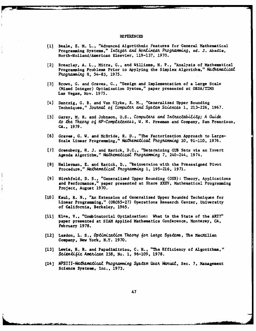
REFERENCES
[1] Beale, E. M. L., "Advanced Algorithmic Features for General MathematicalProgramming Systems," IntegeA and NonineaA PtogAaming, ed. J. Abadie,North-Holland/American Elsevier, 119-137, 1970.
[2] Brearley, A. L., Mitra, G., and Williams, H. P., "Analysis of MathematicalProgramming Problems Prior to Applying the Simplex Algorithm," Ma-hemat eaProgAamtwng 8, 54-83, 1975.
[3] Brown, G. and Graves, G., "Design and Implementation of a Large Scale(Mixed Integer) Optimization System," paper presented at ORSA/TIMSLas Vegas, Nov. 1975.
[4] Dantzig, G. B. and Van Slyke, R. M., "Generalized Upper BoundingTechniques," JOuua oJ Compuwto and Sy4tem ScienceA 1, 213-226, 1967.
[51 Garey, M. R. and Johnson, D.S., Compateu and In~tactabiZity; A Guideto the TheoMy o6 NP-Com~eteneh4, W. H. Freeman and Company, San Francisco,CA., 1979.
[6] Graves, G. W. and McBride, R. D., "The Factorization Approach to Large-Scale Linear Programming," Mathenwti4t Pogamming 10, 91-110, 1976.
[7] Greenberg, H. J. and Rarick, D.C., "Determining GUB Sets via an InvertAgenda Algorithm," Ma-thematcaL Pogamiing 7, 240-244, 1974.
[8] Hellerman, E. and Rarick, D., "Reinversion with the Preassigned PivotProcedure," MathemaicaL PogAaming 1, 195-216, 1971.
[9] Hirshfeld, D. S., "Generalized Upper Bounding (GUB): Theory, Applicationsand Performance," paper presented at Share XXXV, Mathematical ProgrammingProject, August 1970.
[10] Kaul, R. N., "An Extension of Generalized Upper Bounded Techniques forLinear Programming," (ORC65-27) Operations Research Center, Universityof California, Berkeley, 1965.
[11] Klos, V., "Combinatorial Optimization: What is the State of the ART?"paper presented at SIAM Applied Mathematics Conference, Monterey, CA,February 1978.
[12] Lasdon, L. S., Optmization TheoLy 6o LAge S.tem6, The MacMillanCompany, New York, N.Y. 1970.
[13] Lewis, H. R. and Papadimitriou, C. H., "The Efficiency of Algorithms,"Saentidic AmieA2an 238, No. 1, 96-109, 1978.
[15] McBride, R. D., '"inear Prograning with Linked Lists and AutomaticGuberization," Working Paper No. 8175, University of Southern California,School of Business, July 1975.
[16] Sarquis, J., "Converting Linear Models to Network Models," Ph.D.Dissertation, UCLA (December 1979).
[17] Senju, S. and Toyoda, Y., "An Approach to Linear Programing with 0-1Variables," Management Science 15, B196-B207, 1968.
[18] Thomen, D., "Automatic Factorization of Generalized Upper Bounds inLarge Scale Optimization Problems," M.S. Thesis, Naval PostgraduateSchool (September 1979).
[19] Wright, W., M.S. Thesis, Naval Postgraduate School (in preparation).
[20] Zaks, S. (Private Communication, September 1979).
48
DISTRIBUTION LIST
NO. OF COPIES
Defense Documentation Center 2Cameron StationAlexandria, VA 22314
Library, Code 0142 2Naval Postgraduate SchoolMonterey, CA 93940
Dean of Research 1Code 012Naval Postgraduate SchoolMonterey, CA 93940
Library, Code 55 1Naval Postgraduate SchoolMonterey, CA 93940