Elucidating Model Inadequacies in a Cloud Parameterization by Use of anEnsemble-Based Calibration Framework
JEAN-CHRISTOPHE GOLAZ
UCAR Visiting Scientist Program, NOAA/Geophysical Fluid Dynamics Laboratory, Princeton, New Jersey
VINCENT E. LARSON
University of Wisconsin—Milwaukee, Milwaukee, Wisconsin
JAMES A. HANSEN
Naval Research Laboratory, Monterey, California
DAVID P. SCHANEN AND BRIAN M. GRIFFIN
University of Wisconsin—Milwaukee, Milwaukee, Wisconsin
(Manuscript received 28 August 2006, in final form 6 February 2007)
ABSTRACT
Every cloud parameterization contains structural model errors. The source of these errors is difficult topinpoint because cloud parameterizations contain nonlinearities and feedbacks. To elucidate these modelinadequacies, this paper uses a general-purpose ensemble parameter estimation technique. In principle, thetechnique is applicable to any parameterization that contains a number of adjustable coefficients. It opti-mizes or calibrates parameter values by attempting to match predicted fields to reference datasets. Ratherthan striving to find the single best set of parameter values, the output is instead an ensemble of parametersets. This ensemble provides a wealth of information. In particular, it can help uncover model deficienciesand structural errors that might not otherwise be easily revealed. The calibration technique is applied to anexisting single-column model (SCM) that parameterizes boundary layer clouds. The SCM is a higher-orderturbulence closure model. It is closed using a multivariate probability density function (PDF) that repre-sents subgrid-scale variability. Reference datasets are provided by large-eddy simulations (LES) of a varietyof cloudy boundary layers. The calibration technique locates some model errors in the SCM. As a result,empirical modifications are suggested. These modifications are evaluated with independent datasets andfound to lead to an overall improvement in the SCM’s performance.
1. Introduction
Weather and climate models need to simulate a va-riety of boundary layer clouds, such as cumulus, stra-tocumulus, and cumulus-under-stratocumulus. Becausethese clouds are subgrid scale, they must be parameter-ized. Such parameterization packages should be gen-eral enough to simulate any type of cloudy boundarylayer that may develop in a forecast or simulation. The
parameterizations contain approximate equations gov-erning the sources and transport of heat, moisture, andmomentum. Each of these equations contains severalterms, such as the turbulent transport of the quantity ofinterest. Many of the terms must be modeled approxi-mately and hence contain undetermined parameters.
Such parameters are unavoidable. They control, at aminimum, eddy diffusivity and microphysics. Further-more, these parameters cannot be derived theoreticallyfrom first principles. Rather, they must be fitted to dataof some sort, either directly or indirectly. That is, theparameters must be estimated or calibrated (Jackson etal. 2003, 2004; Carrió et al. 2006).
to parameter estimation have resulted in a surge ofinterest in the numerical weather prediction communityand the climate community. For example, ensembleKalman filter (EnKF) methods (Evensen 1994) havebeen used for simultaneous state and parameter esti-mation. Hacker and Snyder (2005) used EnKF to as-similate surface layer observations in a boundary layermodel and estimate the moisture availability param-eter. Aksoy et al. (2006a,b) performed state and param-eter estimation for a two-dimensional sea-breeze modeland numerical weather predictions using the fifth-generation Pennsylvania State University–NationalCenter for Atmospheric Research (PSU–NCAR)Mesoscale Model (MM5). Zupanski and Zupanski(2006) proposed a method to estimate model errorsusing an ensemble data assimilation and state augmen-tation. EnKF methods have also been applied to pa-rameter estimation in climate models of intermediatecomplexity (Annan et al. 2005a,b).
Despite this increased interest, this process of cali-bration has a somewhat sordid reputation in the param-eterization community. Although every cloud param-eterization is calibrated at least informally as a stand-alone single-column model, the calibration of cloudparameterizations is barely discussed in the literature(see, however, Emanuel and Žikovic-Rothman 1999).The reputation of calibration suffers because one oftensuspects that calibration has been used to mask struc-tural model errors. A structural error is a type of modeldeficiency in which there is a misspecification of aterm’s functional form, not merely a misspecification ofa parameter value. This paper argues that the evil hereis not calibration per se, but rather model structuralerror; calibration should not be marginalized, butrather exploited to detect model error.
Two common symptoms of structural error are un-derfitting and overfitting (Geman et al. 1992; Moody1994; Wilks 1995).
Underfitting occurs when a model’s structure is notrich enough to capture true variability in a dataset. Insuch situations, calibration techniques can distinguishtrue structural errors from merely poor parameter val-ues, which are not easy to distinguish otherwise. In onecommon example, a good fit to a data case cannot beachieved despite calibrating all parameter values. Thenthe remaining errors must be structural in some sense.Another more subtle situation occurs when no singleset of parameter values yields a good fit for all cases inthe dataset, even though good parameter values can beobtained for each case separately. In this instance, dif-ferences in the parameter values in the separate cali-brations can provide clues about the source of struc-
tural error. In these situations, calibration does not hideerrors, but exposes them.
Overfitting occurs when too many parameters arefitted using too few data. Overfitting may hide struc-tural errors because it may introduce compensating er-rors between terms. This occurs when, in the process offitting a model to a limited dataset, erroneous param-eter values are inadvertently chosen such that one termcancels structural errors in another. It is nontrivial todetect compensating errors when individual terms arenot directly observed, as is often the case. If the struc-tural errors persist undetected, then the overfittedmodel is unlikely to match other, different datasets. Inthis situation, the model suffers an undesired loss ofgenerality. However, a means to mitigate overfitting iscross validation against independent datasets.
This paper applies an ensemble parameter estimationtechnique to a single-column model (SCM) for bound-ary layer clouds and turbulence. Our two main goalsare to 1) detect structural model errors in the SCM and2) improve the SCM’s fit over a broad range of cloudregimes.
The structure of this paper is as follows. In section 2,we outline the SCM that we calibrate. In section 3, wedescribe our ensemble-based parameter estimationframework. In section 4, we discuss the initial param-eter estimation experiments and the model deficienciesrevealed by them. In section 5, we propose empiricalmodel modifications and test them with referencelarge-eddy simulation (LES) datasets. In section 6, wecross validate these modifications using independentdatasets.
2. Description of SCM
Our SCM simulates boundary layer clouds and isfully described in Golaz et al. (2002a). Briefly, the SCMis a higher-order turbulence closure model that uses amultivariate probability density function (PDF) to closehigher-order turbulence and buoyancy terms. The mul-tivariate PDF represents the horizontal subgrid-scalevariability of vertical velocity, temperature, and totalmoisture. A functional form of the PDF is specified,and for each vertical level and time step, moments forthat functional form are predicted (such as mean, stan-dard deviation, etc.), thus allowing the PDF to varywith height and time. The underlying functional form ofthe PDF is a mixture of two trivariate Gaussians. Theshape was determined empirically from both aircraftmeasurements and LES data by Larson et al. (2002)with further modifications by Larson and Golaz (2005).In Golaz et al. (2002b), the SCM was found to performsatisfactorily over a range of boundary layer regimes
4078 M O N T H L Y W E A T H E R R E V I E W VOLUME 135
comprising clear convection, trade wind shallow cumu-lus, shallow convection over land, and nighttime stra-tocumulus. These regimes were all simulated withoutany case-specific adjustments or trigger functions.Nonetheless, the SCM contains deficiencies whosesources can be difficult to pinpoint.
The deficiencies became more apparent when theSCM was used to simulate a challenging stratocumuluscase, the first research flight (RF01) of the secondDynamics and Chemistry of Marine Stratocumulus(DYCOMS-II) field study (Stevens et al. 2003). RF01was characterized by a strong inversion at cloud top.This inversion was such that stability criteria proposedby Randall (1980) and Deardorff (1980) would havepredicted the cloud to dissipate. However, the cloudwas observed to persist. As was the case for some LESmodels (Stevens et al. 2005), our SCM produced acloud layer that thinned unrealistically over time. Toobtain a more reasonable evolution of the cloud layer(Zhu et al. 2005), we modified the mixing length. Thepresent research was partly motivated by the desire toinvestigate whether the original SCM’s difficulty withthe DYCOMS-II RF01 case was a structural model er-ror or instead a suboptimal choice of parameter values.
3. Ensemble-based parameter estimationframework
Our boundary layer cloud SCM, like most others,contains nonlinear dynamics and multiple parameters.Given this complexity, it can be difficult to predict theconsequences of a particular change in parameter val-ues. This hampers calibration by hand. To expedite theprocess of parameter estimation, we develop an auto-mated calibration framework.
A number of factors guided our choice of a param-eter estimation algorithm:
1) Our single-column model is computationally inex-pensive compared to three-dimensional models, andthe number of parameters we want to estimate ismoderate. Therefore, the efficiency of the param-eter estimation algorithm is not an urgent concern.
2) We wish to use a uniform prior parameter distribu-tion, so as to enable the algorithm to yield the ab-errant parameter values that signal model error.
3) We desire a parameter estimation algorithm that iseasy to use, even for individual scientists who haveexpertise in cloud parameterization but not in pa-rameter estimation.
4) Our source of “data” is LES output that is based onobserved cases. Using LES output as data has twoadvantages: the LES model can be set up identically
to the SCM, and the LES outputs difficult-to-observe fields such as higher-order moments, liquidwater, and cloud fraction. Our goal is limited toemulating LES output, not observational data.Therefore, we treat the LES data as perfect input.Improving the agreement between LES and obser-vations is a separate project that is beyond ourscope.
Our parameter estimation algorithm allows completeflexibility in the choice of field(s) to be optimized andparameter(s) to be estimated. Namely, we can optimizeany combination of prognostic or diagnostic fields pro-duced by the SCM and contained in the LES data. Wecan do so over any time period(s) or altitude range.Furthermore, we can estimate any combination of pa-rameters in the SCM. We can also find overall best-fitparameters for two or more cases (e.g., cumulus andstratocumulus) at once.
Our parameter estimation algorithm for a single en-semble member is as follows. Before beginning the pa-rameter estimation procedure, we select the SCM andLES output fields that we wish to match. Then we de-cide which SCM parameters to calibrate, and we chooseinitial values for these parameters. Then we performthe following steps (see Fig. 1 for a flowchart): run theSCM and evaluate the mismatch between the SCM andLES using a cost function. If the mismatch falls below apredetermined threshold, the algorithm stops. Other-wise, the optimizer chooses a new set of parameter val-ues and the procedure is repeated until convergence.The same procedure is repeated for each ensemblemember but with different initial parameter values.
FIG. 1. Flowchart illustrating the optimization algorithm for asingle ensemble member.
DECEMBER 2007 G O L A Z E T A L . 4079
Central to the parameter estimation algorithm is thechoice of the cost function, J. When errors in the dataare assumed to be Gaussian, the cost function takes thegeneric form:
J�m� � �i�1
N 12N
��g�m� � dobs�TC�1�g�m� � dobs�
Ti,
�1�
where N is the number of observations sets. For eachset, there are M observations represented by the vectordobs. Here g(m) is the corresponding vector of modelpredictions obtained with the model parameter set mand C�1 is the inverse of the covariance matrix. It isoften simplified by only keeping its diagonal elements,namely, the inverse of the squared variances of the ob-servations (e.g., Jackson et al. 2003, 2004). We apply thesame simplification here.
In our application, g(m) is obtained from the SCMoutput [denoted by gSCM(m)] and dobs from the LES“observations” (dLES). Both gSCM(m) and dLES cancomprise any combination of variables produced byboth the SCM and the LES. They could include meanprofiles, such as liquid water potential temperature l,total water mixing ratio qt , cloud fraction, or cloud wa-ter mixing ratio qc. They could also include any one ofthe vertical turbulence moments, such as w�2 or w�3. Anarbitrary number of variables can be included in thecost function. The observations can also include an ar-bitrary number of LES cases (e.g., cumulus and stra-tocumulus). Our reference LES data consist of 1-minaverages. Because the LES fields fluctuate intermit-tently, we do not desire the SCM to mimic a particularLES evolution minute by minute, but rather the LESevolution averaged over a longer time window, typi-cally about 1 h. The specific form of the cost functionbecomes
J�m� � �i�1
Nc
�j�1
N� 1
� i,j2 �
tn
��gSCM�m� � dLEStn
tn�T
� �gSCM�m� � dLEStn
tn��i, j�
�i�1
Nc
�j�1
N� 1
� i, j2 Si, j�m�. �2�
Summations are performed over a number of cases(Nc), variables (N�), and time windows (tn). The over-bar ( )
tn denotes the time-averaging operator applied toa specific time window. Both gSCM and dLES are vectorsthat contain LES and SCM data from every verticallevel within the altitude range of interest. Here Si,j(m)
is the contribution to the error from a combination of aparticular case (i) and variable ( j).
Because we treat the LES observations as perfectinputs for the purpose of calibrating our SCM param-eters, we do not have uncertainties attached to our ob-servations that can be used to estimate the desired vari-ances �i,j. Instead, we set �i,j in Eq. (2) such that con-tributions from each case and each variable have equalweights in the initial value of the cost function:
� i, j2 � Si, j�m0� for i � 1 . . . Nc and j � 1 . . . N� ,
�3�
where Si,j(m0) denotes the initial error contribution.Equation (3) allows us to include disparate variablesand results in each dataset and variable having an equalopportunity at reducing the overall cost function. Notethat this initial weighting could be altered if a modelerhad expert opinion indicating that one case or one vari-able should be overweighed compared to another one.
The optimization algorithm that we use is the down-hill simplex method (Press et al. 1992). The simplexalgorithm is not as efficient as some others, but highefficiency is not our first priority because SCMs arecomputationally inexpensive. For instance, our SCMcan simulate 6 h of cloud evolution within seconds on adesktop personal computer. An additional benefit ofthe method is that it avoids the need to develop a modeladjoint code, thereby greatly simplifying the coding andimplementation. We stress that the choice of a particu-lar optimization scheme is not of fundamental impor-tance. The SCM’s low computational expense allows usto employ other readily available optimizationschemes, such as a conjugate gradient method with fi-nite-difference estimates of the Jacobian.
The minimization of J proceeds on a N-dimensionalsurface, where N is the number of parameters that wewish to estimate. Because of the complexity and dimen-sionality of J, the topology likely consists of a largenumber of local valleys and floors where the minimiza-tion may stop. Therefore, it would be naive to assumethat a single optimization will reach the best minimum.In fact, a single “best” minimum may not even exist;instead, a given function J may possess many compara-bly good minima. For this reason, we choose to performan ensemble of minimizations.
Each ensemble member starts from slightly differentinitial conditions. The initial conditions consist of a sim-plex of N � 1 points on the N-dimensional surface. Forinstance, on a two-dimensional surface, the initial sim-plex is a triangle. The initialization is schematically il-lustrated in Fig. 2 for a two-dimensional case with fourensemble members. For each parameter to be cali-
4080 M O N T H L Y W E A T H E R R E V I E W VOLUME 135
brated, a broad range of values (Pmin,i, Pmax,i) is chosen.The origin of the simplex (P0) lies in the middle of thisparameter space while the remaining vertices are ran-domly chosen by widely perturbing P0 along one par-ticular dimension. This procedure is designed to assumelittle about the parameter values or distributions apriori; that is, we assume an approximately uniformprior parameter distribution. Furthermore, the range(Pmin,i, Pmax,i) applies only to the initial conditions; theoptimization algorithm is free to wander outside thisrange.
Since each ensemble member starts from a slightlydifferent initial simplex, it yields a different optimizedparameter set. This ensemble approach would bewasteful if the model structure were perfect and thetopology of cost function simple: then each ensemblemember would produce identical results. However, thecomplexity of the SCM creates complex structures inthe cost function topology. It is possible to have differ-ent parameter sets that yield similar cost function val-ues. As a result, an ensemble approach is well suitedbecause it can more fully explore the cost functionspace.
Because a single SCM simulation takes on the orderof tens of seconds, the overall computational cost of themethodology is acceptable. An optimization for one
initial set of parameters requires on the order of O(100)iterations before converging. Furthermore, each opti-mization within an ensemble is independent of the oth-ers, thus making the methodology an “embarrassinglyparallel problem” up to the ensemble size.
Our approach to parameter estimation can be cast asan approximation to a Bayesian stochastic inversionwith a uniform prior parameter distribution (Jackson etal. 2004). Each ensemble member of optimized param-eter values does not represent a random draw from thecorrect posterior distribution, but rather needs to beweighted by its (possibly scaled) likelihood given theLES data. The scaling is necessary to account for inac-curate estimates of data uncertainty. We approximatethis scaled weighting below by using the 20 ensemblemembers with the highest likelihood (lowest cost func-tion value). This represents a suboptimal weighting thatwill produce biases in the estimates of the posteriordistribution, but we feel that the inaccuracy is unimpor-tant for our qualitative application.
4. Initial parameter estimation experiments
a. Configuration
A total of 10 parameters from the SCM have beenselected for the initial calibration: C1, C2, C5, C6, C7, C8,C11, �, �2
w, and �. The initial mean values of the 10parameters and their allowable range at the initial timeare listed in Table 1. The actual model equations inwhich all these parameters occur can be found in Golazet al. (2002a) and Larson and Golaz (2005). For conve-nience, the prognostic equations are also listed in theappendix. The C1 controls the dissipation rate of thevertical velocity variance w�2. The C2 controls the dis-
FIG. 2. Illustration of the ensemble initialization procedure fora two-dimensional problem. The hatched triangles represent theinitial simplex for four different ensemble members. They are allcentered around the same point P0. Points P1 and P2 are randomlyperturbed along the first and second dimension, respectively, suchthat they fall within the allowable initial range (Pmin,j, Pmax,j).
TABLE 1. Initial values and ranges of the 10 parameters for theinitial calibration experiments. Also shown are the model vari-ables or components directly affected by these parameters.
C8 w�3 (pressure term) 2.5 1.0 4.0C11 w�3 (pressure term) 0.5 0.1 0.9� PDF functional form 1.25 0.5 2.0� 2
w PDF functional form 0.35 0.3 0.4� (�10�4 s�1) Mixing length 6.0 4.0 8.0
DECEMBER 2007 G O L A Z E T A L . 4081
sipation rates of the scalar variances and covariance q�2t ,
�2l , and q�t �l . The C5 appears in the parameterization of
the pressure correlation term in the w�2 equation. BothC6 and C7 appear in the pressure correlation terms ofthe scalar flux equations w�q�t and w��l . Both C8 andC11 are part of the pressure term parameterization inthe third moment vertical velocity w�3. The parameters� and �2
w arise from the PDF functional form. The �appears in the diagnostic relationship linking the skew-ness of l and qt to the predicted skewness of w. The �2
w
controls the width of the individual Gaussians in thePDF. Finally, � is a mixing time scale used in the com-putation of the mixing length.
Initially, we estimate parameter values for twoboundary layer cloud regimes separately. The differ-ences in parameter values help reveal model structuralerrors. Then we estimate parameter values for bothcases simultaneously. Both cases were previously simu-lated in LES intercomparisons of the Global Water andEnergy Experiment (GEWEX) Cloud System StudiesWorking Group 1 (GCSS-WG1). The setup of bothcases is based on observations. The first regime is atrade wind cumulus regime based on the BarbadosOceanographic and Meteorological Experiment(BOMEX; Siebesma et al. 2003). The second is a ma-rine stratocumulus case, DYCOMS-II RF01, hereafterreferred to as RF01 (Stevens et al. 2005). For each case,the SCM is calibrated against LES results obtained witha version of the Coupled Ocean–Atmosphere Mesos-cale Prediction System (COAMPS) that is suitablymodified for LES scales, which we call “COAMPS–LES” (Golaz et al. 2005). The COAMPS–LES resultslook similar to other LES results in the intercompari-sons. BOMEX and RF01 are selected because they rep-resent different ends of the boundary layer cloud re-gime spectrum. We calibrate only two cases in order toavoid overfitting.
The variables appearing in the cost function in (2) arechosen to be cloud fraction and cloud water mixingratio. Because a major goal of the SCM is to producerealistic clouds, the selection of these cloud variables isnatural. The time windows tn are as follows. BOMEX isa 6-h-long simulation, and we select three 1-h windows,consisting of the fourth, fifth, and sixth simulationhours. RF01 is a 4-h-long simulation, and we select thethird and fourth hours as time windows. The initial ex-periments we present consist of three ensembles: onethat uses BOMEX data exclusively (B1) in the optimi-zation, a second that uses only RF01 data (D1), and athird that combines both BOMEX and RF01 (BD1).Each experiment consists of an ensemble of 400 mem-bers. A complete list of all experiments is provided inTable 2.
b. Results
Results of the initial parameter estimation experi-ments are shown as scatterplots in Fig. 3. In the scat-terplots, each dot represents one ensemble member.The dots are color coded by experiment: green forBOMEX (B1), red for RF01 (D1), and blue for thecombined experiment (BD1). The horizontal axes rep-resent the final parameter value, and the vertical axesrepresent the normalized cost function end value: J �J/Jmin, where Jmin is the lowest cost function value of theensemble. Here Jmin is computed separately for eachensemble. Therefore, the best fitting members (as mea-sured by J) within a given ensemble reside on the lowerportion of each panel, and the worst reside in the upperportion.
For each of the 10 parameters, the scatterplots reveala surprisingly large spread in the final parameter valuescompared to the initial range (gray shaded area). Theplots clearly illustrate the implausibility of finding aglobal minimum that is substantially better than otherlocal minima and justifies the use of an ensemble-basedoptimization approach. For a number of parameters,the posterior parameter distribution is actually widerthan the prior distribution. This seems counterintuitiveat first, but it results from the fact that parameter valuescovary with each other. The product of the optimiza-tion is really an ensemble of parameter sets drawn froma single 10-dimensional distribution and not indepen-dent parameters drawn from 10 separate 1D distribu-tions. Scatterplots can only depict the marginal projec-tions of this multidimensional distribution and cannotreveal how parameters covary. Therefore, changing oneand only one parameter value to another arbitraryvalue within the range of the scatterplot is likely toworsen the fit, because it would neglect the covariationwith other parameters. Also, because of this covariationbetween parameters, it would not be justifiable to selectthe mean of each marginal parameter distribution as anoptimum parameter value. Identification of the covari-
TABLE 2. Summary of all ensemble-based parameter estimationexperiments. Cloud fraction is abbreviated as c.
Category Name SizeNo. of
parameters LES casesLESfields
Initial B1 400 10 BOMEX c, qc
D1 400 10 RF01 c, qc
BD1 400 10 BOMEX andRF01
c, qc
Revised B2 400 14 BOMEX c, qc
D2 400 14 RF01 c, qc
BD2 400 14 BOMEX andRF01
c, qc
4082 M O N T H L Y W E A T H E R R E V I E W VOLUME 135
ance between parameters is a benefit of the ensembleapproach that is not exploited in the current work. Un-derstanding how best to utilize the covarying informa-tion is the subject of ongoing research.
It is also interesting to note that some parametervalues lie outside their physically expected range. Spe-cifically, C5, C7, C8, and C11 are expected to be positivebut are negative in some optimization runs. Our algo-rithm does not explicitly restrict the range of parametervalues, except when the values numerically destabilize
the SCM, in which case the cost function is set to a largepenalty value.
The optimized parameter distribution reveals someunexpected features. For some parameters, the distri-butions for BOMEX (green dots) and RF01 (red dots)overlap considerably, whereas other parameter distri-butions overlap only slightly. In particular, note thesmall overlap between green and red dots for C7 andC11. This small overlap indicates underfitting, which issymptomatic of model structural error.
FIG. 3. Results of the initial parameter estimation experiments (B1, D1, and BD1). Eachpanel represents 1 of the 10 parameters. The horizontal axis is the final parameter value, andthe vertical axis the normalized error, J, of a given optimization with respect to the bestmember of the ensemble. Each optimization is represented by a single dot. Green dots are forthe BOMEX ensemble (B1), red dots are for the RF01 ensemble (D1), and blue dots are forthe combined ensemble (BD1). The gray shaded areas indicate the initial allowable parameterranges.
DECEMBER 2007 G O L A Z E T A L . 4083
Figure 4 displays the same results using standard boxplots. Because the quality of the parameter sets canvary substantially between the best and the worst en-semble member, we focus only on the 20 best ensemblemembers for each experiment. The parameters are nor-malized by their initial values to show their relativedeparture. These box plots clearly reveal that the cali-bration experiments for BOMEX and RF01 tend tofavor different values for C7 and C11. Parameter valuesfor the combined experiment lie in between.
Profiles from the SCM simulations using the 20 bestparameter sets are depicted in Figs. 5 and 6. The pro-
files shown are mean liquid water potential tempera-ture (l), mean total and cloud water mixing ratios (qt,qc), cloud fraction, and the second and third centralmoments of the vertical velocity (w�2, w�3). For BOMEX(Fig. 5), the calibrated SCM runs are able to adequatelyreproduce the LES profiles. Note that only the cloudfraction and qc enter the definition of the cost functionJ. The l, qt , w�2, w�3 are not directly driven to matchthe corresponding LES profiles. This shows that rea-sonable physical constraints are embedded in the SCM.However, none of the simulations accurately repro-duces the cloud fraction near the cloud base. This ap-
FIG. 4. Distributions of the final parameter values for the 20 lowest J ensemble members ofthe initial parameter estimation experiments (B1, D1, and BD1). The values are normalizedby the initial parameter value to show the departure of the end value compared to the initialvalue. Each box plot shows the minimum, first quartile, median, third quartile, and maximumvalues of the distribution.
4084 M O N T H L Y W E A T H E R R E V I E W VOLUME 135
FIG. 5. Comparison of the COAMPS–LES profiles (black) with the 20 lowest J value SCMsimulations for the BOMEX ensemble (B1, green) and combined ensemble (BD1, blue) of theinitial parameter estimation experiments. Profiles shown are liquid water potential tempera-ture (l), total and cloud water mixing ratios (qt, qc), cloud fraction, and second and thirdmoments of the vertical velocity (w�2, w�3). They are averaged over the last 3 h of thesimulation. The gray-shaded areas indicate the range (minimum and maximum bounds) ofother LES models from the intercomparison.
DECEMBER 2007 G O L A Z E T A L . 4085
pears to be a manifestation of a model deficiency thatcannot be corrected by simple parameter recalibration.The differences between the SCM members obtainedfrom the BOMEX experiment (B1, green) and thecombined one (BD1, blue) show larger values of liquid
water and to a lesser degree cloud fraction for the com-bined experiments while the other profiles remain com-parable.
The RF01 profiles paint a different picture (Fig. 6).Even though cloud water for the DYCOMS RF01 en-
FIG. 6. Same as in Fig. 5, but for RF01. Red lines are SCM results from the RF01 ensemble(D1) and blue lines are from the combined ensemble (BD1). Profiles are averaged over thelast simulation hour. LES model range is shown with gray-shaded areas, where available.
4086 M O N T H L Y W E A T H E R R E V I E W VOLUME 135
semble (D1, red) and the combined ensemble (BD1,blue) appear comparable, some significant differencesare present in other fields. In particular, the combinedensemble has difficulties reproducing the profiles of qt
and w�3. The SCM is unable to produce a well-mixedtotal water profile, an indication of a poor representa-tion of boundary layer mixing processes. The w�3 isunrealistically negative in the lower portion of the do-main.
The differences between C7 and C11 values inBOMEX and RF01 warrant further discussion. The C7
appears in the pressure correlation term for the turbu-lence fluxes w�q�t and w��l :
�w�q�t�t �
pressure �
1�0
q�t�p�
�z
� �C6
�w�q�t � C7��w�q�t
�w
�z�
g
�0q�t����,
�4�
�w���l�t �pressure
�1�0
��l�p�
�z
� �C6
�w���l � C7��w���l
�w
�z�
g
�0��l����.
�5�
The C11 enters in the parameterization of the pressurecorrelation term of w�3:
�w�3
�t�
pressure �
3�0
w�2�p�
�z
� �C8
��C8bSkw
4 � 1�w�3
� C11��3w�3�w
�z�
3g
�0w�2����. �6�
Each of the pressure correlation parameterizationsabove contains three terms: the first term is a Newto-nian damping term, the second term is proportional to�w/�z and is generally negligible, and the third term isproportional to the relevant buoyancy moment. TheNewtonian term is sometimes called a “return to isot-ropy” or “slow” term. It always has the opposite sign ofthe prognosed moment and therefore acts as a sink. Thelast two terms are sometimes called “rapid” terms(Pope 2000). The buoyancy term can act as a sink or asource depending on the sign of the buoyancy moment.
LES data reveal that w�3 and w�2�� usually have the
same sign, making C11 an additional damping term. Cu-mulus layers have large skewness values, and thesemust be permitted by the SCM in order to obtain rea-sonable cloud properties. To accomplish this, theBOMEX calibration experiment reveals that the SCMneeds reduced pressure damping and hence smaller C11
values. For stratocumulus, the skewness tends to besmall due to the near symmetry between updraft anddowndraft velocities. Maintaining low skewness inRF01 is aided by larger C11 values.
The role of the C7 term is more complicated. Thebuoyancy contribution to the pressure correlation termin Eqs. (4) and (5) is largest in the upper portion of thecloud layer, both for BOMEX and RF01, near an in-version. The inversion is weak and several hundredmeters deep for BOMEX, but very sharp and shallowfor RF01. Physically, rising eddies are impeded in theirascent by the presence of the inversion. The kineticenergy of impeded updrafts is redistributed from thevertical to the horizontal by the pressure correlationterms. As a result, the buoyancy contribution to thepressure term strongly affects the turbulence fluxesw�q�t and w��l near the inversion and thereby cloud-topmixing. As shown by LESs, RF01 is particularly sensi-tive to cloud-top mixing and entrainment (Stevens et al.2005). The tight coupling between cloud-top mixingand C7 is the likely cause of RF01’s preference forlower values of C7, as revealed by the calibrations.
c. Summary
The initial calibration experiments have revealedthat the SCM simulations agree relatively well with thereference LES for both BOMEX and RF01, if the SCMuses separately calibrated parameter values. A reason-able time evolution of RF01 can also be simulated with-out having to change the mixing length formulation, afinding that was not at all obvious before the experi-ments were performed.
However, the experiments clearly demonstrate thatimproved BOMEX and RF01 require different valuesof the parameters C7 and C11. This is undesirable sincethe SCM is intended to serve as a general boundarylayer parameterization. We address this issue further inthe next section.
5. Revised parameter estimation experiments
a. Proposed model modifications
One major difference between BOMEX and RF01,or more generally between shallow cumulus and stra-tocumulus clouds, is the vertical velocity skewness,Skw � w�3/w�2 3/2
. The skewness of w measures the
DECEMBER 2007 G O L A Z E T A L . 4087
asymmetry between updrafts and downdrafts. In shal-low convection, updrafts tend to be narrow and strongand the compensating downdrafts are broad and weak,giving rise to a large positive skewness. For stratocu-mulus, areas and vertical velocities of updrafts anddowndrafts tend to be comparable, which translatesinto small positive or negative skewness values. Basedon the findings of the previous section, we propose toreformulate the parameters C7 and C11 so as to convertthem into skewness-dependent functions:
Equation (7) implies that in the limit of small skewnessmagnitudes, C7 → C7a, and in the limit of large skew-ness, C7 → C7b. The sharpness of the transition betweensmall and large values is controlled by C7c. The form ofthe skewness dependency is illustrated in Fig. 7. Equa-tions (7)–(8) are purely empirical and we make no at-tempt to justify them theoretically. In essence, they aresimple structural modifications that one can conceive toremedy the problems uncovered in the previous sec-tion.
A new set of ensemble-based parameter estimationexperiments is performed using the new formulationsfor C7 and C11 (B2, D2, and BD2 in Table 2). Themethodology is the same as for the initial experiments,but the dimensionality of the optimization problem isnow 14. The range and initial values of the newlyintroduced parameters are given in Table 3. All the
other parameters have the same range and value as inTable 1.
b. Results
The final parameter values of all the members for therevised experiments B2, D2, and BD2 are shown asscatterplots in Fig. 8. The overlap between BOMEX(green points) and RF01 (red points) ensembles for C7x
and C11x is now improved compared to Fig. 3. As acaveat, we note that because the SCM inevitably stillcontains structural errors and because we have opti-mized simultaneously for all parameter values, the op-timized values have undoubtedly been influenced bycompensating errors between terms. Therefore, an op-timal parameter value for a given term in our SCM isnot necessarily optimal for the same term in a differentSCM.
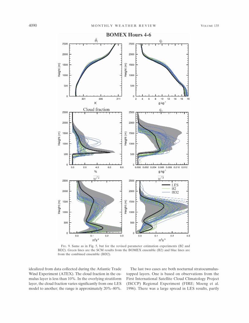
We now focus on the SCM profiles of the 20 bestparameter sets of each ensemble. The profiles from theBOMEX ensemble (B2, green lines; Fig. 9) show littlechange compared to the initial experiment (B1, greenlines; Fig. 5). The cloud water profile is improved in therevised combined experiment (BD2, blue lines), but thecloud fraction is still underestimated near the cloudbase.
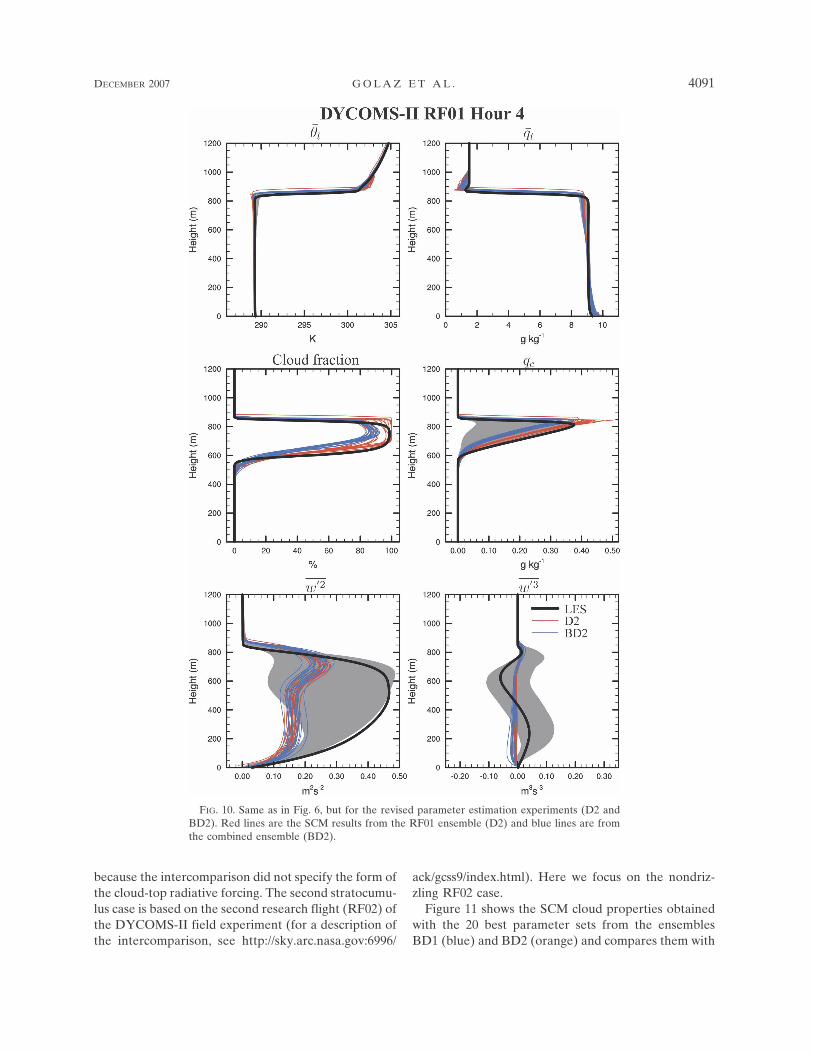
The impact of the modified pressure terms C7 andC11 is more significant for RF01 (Fig. 10). The RF01ensemble (D2) and the combined ensemble (BD2)now both yield SCM results that agree better withCOAMPS–LES. This is in contrast to the initial experi-ments (Fig. 6) in which the RF01 ensemble (D1) pro-duced total water mixing ratio profiles that were notsufficiently well mixed, and had erroneous w�3 profiles.
The results from the BD2 ensemble demonstrate thatthe modifications made to C7 and C11 in Eqs. (7)–(8)allow for the existence of parameter sets that producereasonable results for BOMEX and RF01 simulta-neously. This was not the case with the unmodifiedSCM. Furthermore, before this work was performed, it
FIG. 7. Illustration of the skewness-dependency function of themodified parameters in Eqs. (7)–(8). Different values of the de-nominator in the exponent are plotted for illustration purposes.
TABLE 3. Initial values and ranges of the new parameters for therevised calibration experiments (B2, D2, and BD2). The initialvalues and ranges of the remaining parameters are identical tothose in Table 1.
4088 M O N T H L Y W E A T H E R R E V I E W VOLUME 135
would have been difficult to identify modifications tothe SCM that would have been likely to faithfully simu-late both BOMEX and RF01.
6. Evaluation with independent data
We have intentionally calibrated only two LES casesand reserved other cases for cross validation in order toavoid overfitting. To verify that we have indeedavoided overfitting, we simulate four additional testcases using the 20 best parameter sets from the BD1and BD2 ensembles. The additional test cases are all set
up according to the specifications of GCSS intercom-parisons, which are based loosely on the observations.
The first case is shallow cumulus over land from theSouthern Great Plains (SGP) Atmospheric and Radia-tion Measurement (ARM) site (Brown et al. 2002). Thesimulation starts in the morning with clear skies. As theday progresses, the boundary layer deepens due to thesurface fluxes. Fair-weather cumulus clouds develop,grow progressively during the day, and dissipate beforethe simulation’s end at about sundown.
The second case involves cumulus clouds rising undera broken stratocumulus deck (Stevens et al. 2001). It is
FIG. 8. Same as in Fig. 3, but for the results of the revised parameter estimation experiments (B2, D2, and BD2) with 14 parameters.Green dots are for the BOMEX ensemble (B2), red dots are for the RF01 ensemble (D2), and blue dots are for the combined ensemble(BD2).
DECEMBER 2007 G O L A Z E T A L . 4089
idealized from data collected during the Atlantic TradeWind Experiment (ATEX). The cloud fraction in the cu-mulus layer is less than 10%. In the overlying stratiformlayer, the cloud fraction varies significantly from one LESmodel to another; the range is approximately 20%–80%.
The last two cases are both nocturnal stratocumulus-topped layers. One is based on observations from theFirst International Satellite Cloud Climatology Project(ISCCP) Regional Experiment (FIRE; Moeng et al.1996). There was a large spread in LES results, partly
FIG. 9. Same as in Fig. 5, but for the revised parameter estimation experiments (B2 andBD2). Green lines are the SCM results from the BOMEX ensemble (B2) and blue lines arefrom the combined ensemble (BD2).
4090 M O N T H L Y W E A T H E R R E V I E W VOLUME 135
because the intercomparison did not specify the form ofthe cloud-top radiative forcing. The second stratocumu-lus case is based on the second research flight (RF02) ofthe DYCOMS-II field experiment (for a description ofthe intercomparison, see http://sky.arc.nasa.gov:6996/
ack/gcss9/index.html). Here we focus on the nondriz-zling RF02 case.
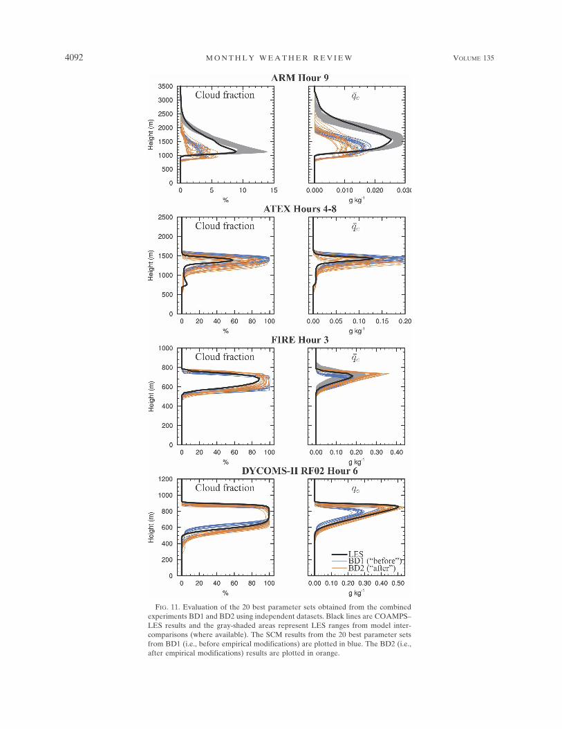
Figure 11 shows the SCM cloud properties obtainedwith the 20 best parameter sets from the ensemblesBD1 (blue) and BD2 (orange) and compares them with
FIG. 10. Same as in Fig. 6, but for the revised parameter estimation experiments (D2 andBD2). Red lines are the SCM results from the RF01 ensemble (D2) and blue lines are fromthe combined ensemble (BD2).
DECEMBER 2007 G O L A Z E T A L . 4091
FIG. 11. Evaluation of the 20 best parameter sets obtained from the combinedexperiments BD1 and BD2 using independent datasets. Black lines are COAMPS–LES results and the gray-shaded areas represent LES ranges from model inter-comparisons (where available). The SCM results from the 20 best parameter setsfrom BD1 (i.e., before empirical modifications) are plotted in blue. The BD2 (i.e.,after empirical modifications) results are plotted in orange.
4092 M O N T H L Y W E A T H E R R E V I E W VOLUME 135
COAMPS–LES (black). The main interest is in com-paring the BD1 and BD2 SCM profiles, which are the“before” and “after” pictures showing the effects of ourempirical modifications.
The biggest difference occurs for RF02, where theBD2 SCM (after) cloud water profiles are markedlysuperior to the BD1 (before) profiles. Most BD1 en-semble members predict liquid water amount near thecloud top that underestimates the LES value by nearly50%. In contrast, the BD2 ensemble members almostexactly match the LES.
The BD2 FIRE cloud properties appear to suffer aslight degradation in BD2 compared to BD1. Given theuncertainties surrounding the specifications of this case,one should be cautious with respect to the significanceof this degradation. For example, a simulation using adifferent LES model produced a liquid water amount of0.25 g kg�1 near the cloud top (Golaz et al. 2002b, theirFig. 12d), much closer to the BD2 values.
For ARM and ATEX, the changes between BD1 andBD2 are modest. ARM results both underestimate thecloud amount compared to the LES. These profiles areactually slightly worse than the results published in Go-laz et al. (2002b). However, since BD1 and BD2 pro-files are qualitatively similar, the degradation does notstem from the SCM modifications we made [Eqs. (7)and (8)], but rather from the values of the parametersthemselves.
On balance, the empirical changes made to C7 andC11 [Eqs. (7) and (8)] are beneficial to RF02, neutral toARM and ATEX, and slightly negative for FIRE.Given that these changes are solely based on BOMEXand RF01 datasets, we can safely state that we haveavoided an overfitting situation and hence can havesome confidence in the generality of the SCM modifi-cations, despite their empirical nature.
7. Conclusions
We have presented an ensemble method of param-eter estimation. It has four chief advantages:
1) It allows complete flexibility in the choice of param-eters to be estimated and fields to be optimized. Forinstance, we may simultaneously estimate any com-bination of the parameters in Tables 1 and 3 (i.e., C1,C2, and so forth). Furthermore, we may optimizeany combination of fields (e.g., cloud fraction andliquid water) that are produced by the SCM andcontained in the LES data.
2) The method is conceptually straightforward.3) The method is easy to implement, because it does
not require writing an adjoint of the model code.
4) The method produces an ensemble of sets of best-fitparameter values. This is useful in cases in which thecost function contains many comparable localminima. The ensemble methodology provides notonly the range of acceptable values of parameters,but also information about how the best-fit param-eter values covary with each other.
We have used the ensemble parameter estimationmethod to calibrate a single-column model (SCM) ofboundary layer clouds. The “data” used are outputfrom six large-eddy simulations (LES). These consist ofthree stratocumulus cases, a trade wind cumulus case, acontinental cumulus case, and a cumulus-under-stratocumulus case. We calibrate 10 SCM parameterssimultaneously against profiles of cloud fraction andliquid water.
In calibrating the SCM, we sought to avoid the op-posing problems of overfitting and underfitting.
To avoid overfitting, we fit only two fields, cloudfraction and liquid water, and two cases, the BOMEXtrade wind cumulus case and the DYCOMS-II RF01marine stratocumulus case. Other fields and cases wereused for cross validation. That is, they were used toverify that the chosen parameter values fit well gener-ally, not merely for the two fields and cases used in thecalibration.
To diagnose the cause of underfitting, we calibratedBOMEX and RF01 separately, thereby obtaining twosets of parameter values. The separate calibrations re-vealed differences in the values of the parameters C7
and C11. Assessing the significance of these differenceswas made possible by the ensemble methodology,which clearly showed the lack of overlap in the accept-able parameter values. This demonstrates that calibra-tion need not obscure model structural error; in fact, ifused strategically, calibration may reveal structural er-rors. We then replaced the parameters C7 and C11 bythe empirical functions of skewness. This structuralmodification ameliorated the underfitting and permit-ted the SCM to model all six cloud cases more accu-rately without case-specific adjustments.
Although the parameter estimation technique canhelp identify the existence of model structural errors, itcannot propose new ideas to fix those errors. Neverthe-less, automated parameter estimation does speed upthe process of model development because it allowsrapid recalibration when a new model improvement isintroduced. This is useful because the introduction of atrue model improvement often produces a worse fit todata, since errors in other parts of the model are nolonger compensated.
A product of the ensemble approach to parameter
DECEMBER 2007 G O L A Z E T A L . 4093
estimation is a covarying distribution of parameter val-ues. In this work we focused only on distributions ofindividual parameter values, but there is likely usefulinformation in the higher moments of the parametricdistribution. Additionally, we never expect our param-eterization to be perfect, and the distribution of param-eter values provides information about how parametersneed to be altered to mimic inadequacies in the model.These distributions could potentially be exploited todevelop stochastic parameterizations for use in en-semble forecast integrations.
In general, ensemble parameter estimation tech-niques are applicable to a wide range of other param-eterizations, such as land surface (Jackson et al. 2003)or deep convective parameterizations (Emanuel andŽikovic-Rothman 1999). Also, general circulation mod-els may benefit in the future, when computationalpower has increased. A single cloud parameterizationcontaining subparameterizations for each term is analo-gous to a single climate model containing different pa-rameterizations for radiative transfer, gravity wavedrag, and so forth. Both suffer the problem of compen-sating errors and model structural errors, and both maybenefit from tools to diagnose those errors.
Acknowledgments. COAMPS is a registered trade-mark of the Naval Research Laboratory. J.-C. Golazwas supported by the Visiting Scientist Program at theNOAA/Geophysical Fluid Dynamics Laboratory, ad-ministered by the University Corporation for Atmo-spheric Research (UCAR). V. E. Larson, D. P.Schanen, and B. M. Griffin are grateful for financialsupport provided by Grant ATM-0442605 from the Na-tional Science Foundation, and by Subaward G-7424-1from the DoD Center for Geosciences/AtmosphericResearch at Colorado State University via CooperativeAgreement DAAD19-02-2-0005 with the Army Re-search Laboratory. J. A. Hansen acknowledges supportfrom ONR YIP N00014-02-1-0473. C. Jackson is ac-knowledged for a useful discussion about this work.
APPENDIX
Model Predictive Equations
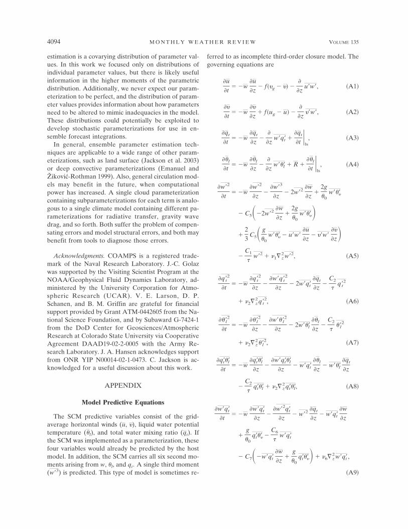
The SCM predictive variables consist of the grid-average horizontal winds (u, �), liquid water potentialtemperature (l), and total water mixing ratio (qt). Ifthe SCM was implemented as a parameterization, thesefour variables would already be predicted by the hostmodel. In addition, the SCM carries all six second mo-ments arising from w, l, and qt . A single third moment(w�3) is predicted. This type of model is sometimes re-
ferred to as incomplete third-order closure model. Thegoverning equations are
�u
�t� �w
�u
�z� f��g � �� �
�
�zu�w�, �A1�
��
�t� �w
��
�z� f�ug � u� �
�
�z��w�, �A2�
�qt
�t� �w
�qt
�z�
�
�zw�q�t �
�qt
�t �ls, �A3�
��l
�t� �w
��l
�z�
�
�zw���l � R �
��l
�t �ls, �A4�
�w�2
�t� �w
�w�2
�z�
�w�3
�z� 2w�2
�w
�z�
2g
�0w����
� C5��2w�2�w
�z�
2g
�0w�����
�23
C5� g
�0w���� � u�w�
�u
�z� ��w�
��
�z��
C1
�w�2 � 1z
2w�2, �A5�
�qt�2
�t� �w
�qt�2
�z�
�w�qt�2
�z� 2w�q�t
�qt
�z�
C2
�qt�
2
� 2z2qt�
2, �A6�
�� l�2
�t� �w
�� l�2
�z�
�w�� l�2
�z� 2w���l
��l
�z�
C2
�� l�
2
� 2z2� l�
2, �A7�
�q�t��l�t
� �w�q�t��l
�z�
�w�q�t��l�z
� w�q�t��l
�z� w���l
�qt
�z
�C2
�q�t��l � 2z
2q�t��l, �A8�
�w�q�t�t
� �w�w�q�t
�z�
�w�2q�t�z
� w�2�qt
�z� w�q�t
�w
�z
�g
�0q�t��� �
C6
�w�q�t
� C7��w�q�t�w
�z�
g
�0q�t���� � 6z
2w�q�t ,
�A9�
4094 M O N T H L Y W E A T H E R R E V I E W VOLUME 135
�w���l�t
� �w�w���l
�z�
�w�2��l�z
� w�2��l
�z
� w���l�w
�z�
g
�0��l��� �
C6
�w���l
� C7��w���l�w
�z�
g
�0��l���� � 6z
2w���l,
�A10�
�w�3
�t� �w
�w�3
�z�
�w�4
�z� 3w�2
�w�2
�z� 3w�3
�w
�z
�3g
�0w�2��� �
C8
��C8bSkw
4 � 1�w�3
� C11��3w�3�w
�z�
3g
�0w�2����
� �Kw � 8�z2w�3, �A11�
where R is the radiative heating rate, f is the Coriolisparameter, and ug and �g are the geostrophic winds.Here (�qt /�t) | ls and (�l /�t) | ls are large-scale moistureand temperature forcings, respectively. Here g is thegravity, and �0 and 0 are the reference density andpotential temperature, respectively. For additional de-tails, the reader is referred to Golaz et al. (2002a). ThePDF functional form used to close the buoyancy andhigher-order moments follows Larson and Golaz(2005). One exception is the treatment of the PDF pa-rameter �2
w. Instead of using Eq. (37) in Larson andGolaz (2005), we keep �2
w constant but include it in thelist of parameters to be calibrated.
Some aspects of the numerical integration havechanged compared to Golaz et al. (2002a). Manyhigher-order turbulence moments are now discretizedsemi-implicitly to improve numerical stability and allowfor longer time steps. Equations (A6)–(A8) are nowsolved for their steady-state solutions, thus makingthem diagnostic. The form of the damping term in(A11) has been altered. The change does not impactthe results significantly, but it allows for a semi-implicitnumerical treatment, which improves stability.
REFERENCES
Aksoy, A., F. Zhang, and J. W. Nielsen-Gammon, 2006a: En-semble-based simultaneous state and parameter estimation ina two-dimensional sea-breeze model. Mon. Wea. Rev., 134,2951–2970.
——, ——, and ——, 2006b: Ensemble-based simultaneous stateand parameter estimation with MM5. Geophys. Res. Lett., 33,L12801, doi:10.1029/2006GL026186.
Annan, J. D., J. C. Hargreaves, N. R. Edwards, and R. Marsh,2005a: Parameter estimation in an intermediate complexity
earth system model using an ensemble Kalman filter. OceanModell., 8, 135–154.
——, D. J. Lunt, J. C. Hargreaves, and P. J. Valdes, 2005b: Pa-rameter estimation in an atmospheric GCM using the En-semble Kalman Filter. Nonlinear Processes Geophys., 12,363–371.
Brown, A. R., and Coauthors, 2002: Large-eddy simulation of thediurnal cycle of shallow cumulus convection over land. Quart.J. Roy. Meteor. Soc., 128, 1075–1093.
Carrió, G., W. R. Cotton, and D. Zupanski, 2006: Data assimila-tion into a LES model: Retrieval of IFN and CCN concen-trations. Preprints, 12th Conf. on Cloud Physics, Madison,WI, Amer. Meteor. Soc., 1.4A.
Deardorff, J. W., 1980: Cloud top entrainment instability. J. At-mos. Sci., 37, 131–147.
Emanuel, K. A., and M. Žikovic-Rothman, 1999: Developmentand evaluation of a convection scheme for use in climatemodels. J. Atmos. Sci., 56, 1766–1782.
Evensen, G., 1994: Sequential data assimilation with a nonlinearquasi-geostrophic model using Monte Carlo methods to fore-cast error statistics. J. Geophys. Res., 99, 10 143–10 162.
Geman, S., E. Bienenstock, and R. Doursat, 1992: Neural net-works and the bias/variance dilemma. Neural Comput., 4,1–58.
Golaz, J.-C., V. E. Larson, and W. R. Cotton, 2002a: A PDF-based model for boundary layer clouds. Part I: Method andmodel description. J. Atmos. Sci., 59, 3540–3551.
——, ——, and ——, 2002b: A PDF-based model for boundarylayer clouds. Part II: Model results. J. Atmos. Sci., 59, 3552–3571.
——, S. Wang, J. D. Doyle, and J. M. Schmidt, 2005: COAMPS®-LES: Model evaluation and analysis of second and third mo-ment vertical velocity budgets. Bound.-Layer Meteor., 116,487–517.
Hacker, J. P., and C. Snyder, 2005: Ensemble Kalman filter as-similation of fixed screen-height observations in a parameter-ized PBL. Mon. Wea. Rev., 133, 3260–3275.
Jackson, C., Y. Xia, K. Sen, and P. L. Stoffa, 2003: Optimal pa-rameter and uncertainty estimation of a land surface model:A case study using data from Cabauw, Netherlands. J. Geo-phys. Res., 108, 4583, doi:10.1029/2002JD002991.
——, M. K. Sen, and P. L. Stoffa, 2004: An efficient stochasticBayesian approach to optimal parameter and uncertainty es-timation for climate model predictions. J. Climate, 17, 2828–2841.
Larson, V. E., and J.-C. Golaz, 2005: Using probability densityfunctions to derive consistent closure relationships amonghigher-order moments. Mon. Wea. Rev., 133, 1023–1042.
——, ——, and W. R. Cotton, 2002: Small-scale and mesoscalevariability in cloudy boundary layers: Joint probability den-sity functions. J. Atmos. Sci., 59, 3519–3539.
Moeng, C.-H., and Coauthors, 1996: Simulation of a stratocumu-lus-topped planetary boundary layer: Intercomparisonamong different numerical codes. Bull. Amer. Meteor. Soc.,77, 261–278.
Moody, J., 1994: Prediction risk and architecture selection forneural networks. From Statistics to Neural Networks: Theoryand Pattern Recognition Applications, V. Cherkassky, J. H.Friedman, and H. Wechsler, Eds., NATO ASI Series F, Vol.136, Springer-Verlag, 143–156.
Pope, S. B., 2000: Turbulent Flows. Cambridge University Press,771 pp.
Press, W. H., S. A. Teukolsky, W. T. Vetterling, and B. P. Flan-
DECEMBER 2007 G O L A Z E T A L . 4095
nery, 1992: Numerical Recipes in FORTRAN: The Art of Sci-entific Computing. 2d ed. Cambridge University Press, 965 pp.
Randall, D. A., 1980: Conditional instability of the first kind up-side-down. J. Atmos. Sci., 37, 125–130.
Siebesma, A. P., and Coauthors, 2003: A large eddy simulationintercomparison study of shallow cumulus convection. J. At-mos. Sci., 60, 1201–1219.
Stevens, B., and Coauthors, 2001: Simulations of trade wind cu-muli under a strong inversion. J. Atmos. Sci., 58, 1870–1891.
——, and Coauthors, 2003: Dynamics and chemistry of marinestratocumulus—DYCOMS-II. Bull. Amer. Meteor. Soc., 84,579–593.
——, and Coauthors, 2005: Evaluation of large-eddy simulationsvia observations of nocturnal marine stratocumulus. Mon.Wea. Rev., 133, 1443–1462.
Wilks, D. S., 1995: Statistical Methods in the Atmospheric Sciences.Academic Press, 467 pp.
Zhu, P., and Coauthors, 2005: Intercomparison and interpretationof single-column model simulations of a nocturnal stratocu-mulus-topped marine boundary layer. Mon. Wea. Rev., 133,2741–2758.
Zupanski, D., and M. Zupanski, 2006: Model error estimationemploying an ensemble data assimilation approach. Mon.Wea. Rev., 134, 1337–1354.
4096 M O N T H L Y W E A T H E R R E V I E W VOLUME 135