19
EM propagation paths 1/17/12
| Date post: | 29-Dec-2015 |
| Category: |
Documents |
| Upload: | sheila-atkins |
| View: | 221 times |
| Download: | 1 times |

EM propagation paths
1/17/12

Introduction• Motivation: For all remote sensing instruments, an understanding
of propagation is necessary to properly interpret the measurements.• EM waves propagate as straight lines at the speed of light (c) (recall
Maxwell’s Eqs.)
0 and 0 are the electrical permittivity and magnetic inductive capacity of free space, and are wavelength & frequency
• The atmosphere modifies EM propagation: 1, is larger than 0, and furthermore, 1 is a function of height. Speed of propagation is
• The waves bend in the atmosphere (the process of refraction) due to the variation of 1(xi) = 1(x,y,z).
• Note atmos 1 (>0), and therefore v < c

Refractive index of air• Index of refraction, n, is defined as the ratio of the speed of light in a
medium to that in a vacuum:
• n is is dependent on the density and polarization of molecules
• O2 and N2 are not polarized, but they can become polarized in the presence of an imposed electric field.
• For no external forces, the orientation of H2O molecules is random due to thermal agitation. However, if H2O subjected to an E field, then it is aligned so that the dipole fields add constructively to enhance the net electric force on each H2O molecule.
• This behavior is related to the extraction of energy from the incident wave and leads to attenuation (e.g., 95 GHz)

• permittivity of a gas depends on molecular number density, N, multiplied by a factor T proportional to the molecule’s level of polarization, expressed by the Lorenz-Lorentz formula
• r is the relative permittivity, r = /0 = n2. • For air, the value of r is 1.000300, and the above formula can be
rewritten as
• For the atmosphere which is a mixture of molecules, the following equation applies:
• mass density is related to the number density N by the molecular weight M:
• Normalized equation of state for a gas, for standard temperature (273 K) and pressure (1013.25 mb)

• From Avogadro’s Law, the number of molecules per unit volume of gas is given as
• and the number for an arbitrary T and p is
• The last (3rd) term on the rhs represents the contribution from the permanent dipole moment of water vapor
(3.3)

Refractivity• Define:• From the above, n becomes• Expansion in a Taylor’s series:• Using (3.3):
• cd = 77.6 K mb-1, cw1 = 71.6 K mb-1, cw2 = 3.7 x 10⁵ K2 mb-1
• (2.17) can be approximated as
• Example: e = 10 mb, p = 1000 mb, T = 300 KN = 0.26(103 + 1.6x10²) = 300n = 1 + Nx10-6 = 1.000300
• The value of n in the atmosphere differs little from that of free space, but this small difference, and the variation with height, is important to EM propagation.
(2.17)

N normally decreases with altitude, since both p and T decrease with altitude, on the average, and p dereases at a more rapid rate (i.e., the fractional decrease is much larger).
When dN/dz < -157 km-1 (the case for inversion layers), EM rays are bent toward the earth’s surface.
Small scale fluctuations in N Bragg scattering (discussed later).
We will first consider quasi-horizontal layers of N and how dN/dz affects EM propagation in the atmosphere.

Spherically-stratified atmosphere• Assume T and e (RH) are horizontally homogeneous so that N =
N(z).
• A ray path in spherically stratified atmosphere is given by the differential equation
• Whose solution is

The variable s(z) is the great circle distance to a point directly below the ray at height h above the surface, a is the earth’s radius, R is the radial distance from the center of the earth, and is elevation angle of the radar antenna.
We also assume:n(z) is smoothly changing so that ray theory is applicablen(0) is the refractivity at the radar site

Aside: Snell’s Law• The variation of a ray path with a change in refractive index is
given by
In the atmosphere, n decreases with height, and therefore the rays are bent toward the earth (as in the figure above).

Equivalent earth model
Several simplifications can be applied to (3.5):
a) Small angle approximation: << 1
b) Large earth approximation: z << R
Then the approximate equations describing the path of ray at small angles relative to the earth are:

The index of refraction for the standard atmosphere is dn/dz = const = -4 x 10⁻⁸ m-1.
For the standard atmosphere, one can define a fictitious earth curvature where rays propagating relative to the fictitious earth are straight lines, as follows:

The height of a ray as a function of slant range for zero elevation angle is given by
(3.7)
This relation assumes that:a) n is linearly dependent on hb) The development of Eq. (3.7) assumed dz/ds <<1,
which imposes a limit on the use of an effective earth radius

The vertical gradient of n is typically not constant, and appreciable departures from linearity exist in the vicinity of temperature inversions and large vertical gradients in water vapor. The departure between the 4/3 earth radius model and a reference atmosphere is shown in Fig. 2.7 below. In each model, the surface value is N = 313. A large difference between these two models exists at heights > 2 km AGL.

For weather radar applications (z < 10 km), and n exhibits a vertical gradient of -1/4a within the lowest one kilometer, the 4/3 earth radius model can be used with sufficient accuracy. Fig. 2.8 reveals a comparison of ray paths for two models: the 4a/3 model, and an exponential model of the form
The 4a/3 model works well, except in low level inversions

Standard refractionRinehart provides the following equation to compute beam height when standard refraction applies:
r - slant range , - elevation angle,
H0 - height of the radar antenna
R’ = (4/3)R, R - earth’s radius (6374 km)

Ground-based ducts and reflection heights
The example profile of N shown in Fig. 2.9 illustrates anomalous propagation
and beam distortions. Ray paths are shown in Fig. 2.10
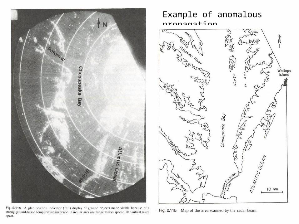
Example of anomalous propagation

Homework
• Do problems 1-3 in the notes.


