P OLICY R ESEARCH WORKING P APER 4897 Emerging Market Fluctuation What Make the Difference Constantino Hevia The World Bank Development Reearch Group Macroeconomic and Growth Team April 2009 WPS4897 Public Disclosure Authorized Public Disclosure Authorized Public Disclosure Authorized Public Disclosure Authorized
Transcript
Policy ReseaRch WoRking PaPeR 4897
Emerging Market Fluctuations�
What Makes� the Difference?�
Constantino Hevia
The World BankDevelopment Res�earch GroupMacroeconomics� and Growth TeamApril 2009
WPS4897P
ublic
Dis
clos
ure
Aut
horiz
edP
ublic
Dis
clos
ure
Aut
horiz
edP
ublic
Dis
clos
ure
Aut
horiz
edP
ublic
Dis
clos
ure
Aut
horiz
ed
Produced by the Res�earch Support Team
Abstract
The Policy Research Working Paper Series disseminates the findings of work in progress to encourage the exchange of ideas about development issues. An objective of the series is to get the findings out quickly, even if the presentations are less than fully polished. The papers carry the names of the authors and should be cited accordingly. The findings, interpretations, and conclusions expressed in this paper are entirely those of the authors. They do not necessarily represent the views of the International Bank for Reconstruction and Development/World Bank and its affiliated organizations, or those of the Executive Directors of the World Bank or the governments they represent.
Policy ReseaRch WoRking PaPeR 4897
Aggregate fluctuations� in emerging countries� are quantitatively larger and qualitatively different in key res�pects� from thos�e in developed countries�. Us�ing data from Mexico and Canada, this� paper decompos�es� thes�e differences� in terms� of s�hocks� to aggregate efficiency and s�hocks� that dis�tort the decis�ions� of hous�eholds� about how much to inves�t, cons�ume, and work in a s�tandard model
This� paper—a product of the Growth and the Macroeconomics� Team, Development Res�earch Group—is� part of a larger effort in the department to unders�tand macroeconomic volatility in developing countries�. Policy Res�earch Working Papers� are als�o pos�ted on the Web at http://econ.worldbank.org. The author may be contacted at [email protected].
of a s�mall open economy. The decompos�ition exercis�e s�ugges�ts� that mos�t of thes�e differences� are explained by fluctuations� in aggregate efficiency, dis�tortions� in labor decis�ions� over the bus�ines�s� cycle, and, mos�t importantly, fluctuations� in country ris�k. Other dis�tortions� are quantitatively les�s� important.
Emerging Market Fluctuations: What Makes the
Di�erence?∗
Constantino Hevia †
∗JEL Codes: E32, F41. Keywords: Business Cycles, Small Open Economy, Country Risk Premium†I thank Aart Kray, Juan Pablo Nicolini, Demian Pouzo, Claudio Raddatz, and Luis Serven for helpful
comments and suggestions. The �ndings, interpretations, and conclusions expressed in this paper are entirely
those of the author. They do not necessarily represent the view of the World Bank, its Executive Directors, or
the countries they represent
1 Introduction
Aggregate �uctuations in emerging countries are di�erent from those in developed countries.
Table 1 illustrates this point. The �rst and second rows of the table display summary statis-
tics of the business cycle in two representative emerging and developed countries, Mexico
and Canada respectively. The third and fourth rows of the table report the same statistics
averaged across 13 emerging and 13 developed countries. Overall, the table shows that, while
economic aggregates are substantially more volatile in emerging countries (except, perhaps,
hours worked), there is a deeper di�erence between these countries: consumption is more
volatile than output in emerging countries but less volatile in developed countries; and the
share of net exports on output is highly countercyclical in emerging countries but less so in
developed countries. Moreover, these regularities hold across a large number of emerging and
developed countries (Neumeyer and Perri, 2005; Aguiar and Gopinath, 2007).
Table 1: Business Cycles in Emerging and Developed Small Open Economies
This table reports second moments of HP-�ltered quarterly aggregate data. The statistics σ(x) and ρ(x, y)measure, respectively, the standard deviation of the series x and the correlation coe�cient between theseries x and y. The variable y denotes output; l, hours worked; m, net exports; c, private consumption; andx, investment. GMM-based standard errors are reported in parentheses.Sources: Rows 1 and 2, author's calculations. Rows 3 and 4 taken from Aguiar and Gopinath (2007).
While researchers agree on these di�erences, they disagree on their causes: by introducing
di�erent frictions and shocks into their models, researchers provide alternative stories for why
aggregate �uctuations in emerging countries are di�erent. (Christiano, Gust, and Roldós,
2004; Neumeyer and Perri, 2005; Mendoza, 2008; Uribe and Yue, 2006; Aguiar and Gopinath,
1
2007; Arellano, 2008, to name but a few.) These frictions and shocks, however, are usually
chosen based on intuition or anecdotal evidence.
The purpose of this paper is to identify the type of reduced form distortions that ex-
plain the observed business cycle di�erences between emerging and developed countries. The
logic of the experiment is as follows. At a conceptual level, shocks and frictions in most
structural models drive a wedge between certain marginal rates of substitution and marginal
rates of transformation relative to a prototype frictionless economy. Then, instead of testing
whether a particular structural model generates the data, I estimate these wedges based on
the prototype economy and measure their contribution to aggregate �uctuations. The esti-
mated wedges, however, cannot be used to identify primitive shocks and frictions: models
with di�erent primitive shocks and frictions could induce movements in the same reduced
form wedge in the prototype economy. Nevertheless, these wedges o�er useful information: a
successful model should induce reduced form wedges similar to those estimated based on the
prototype economy; moreover, these wedges should account, quantitatively, for �uctuations
in the economic aggregates.
Several authors have used variations of this approach applied to the U.S., including Parkin
(1988), Hall (1997), Rotemberg and Woodford (1999), Mulligan (2002), Chari, Kehoe, and
McGrattan (2007), and Shimer (2009). In this paper I follow more closely the methodology
proposed by Chari, Kehoe, and McGrattan, labeled `Business Cycle Accounting'. In this
methodology, the researcher interprets the data through the lens of a small open economy
model. This prototype economy is subject to reduced form shocks that are interpreted literally
as total factor productivity (the e�ciency wedge), as labor and investment taxes (the labor
wedge and investment wedge), as �uctuations in real interest rates (the risk premium wedge),
and as government consumption (the government consumption wedge).
I estimate a stochastic process for these wedges using data from a representative emerging
country, Mexico, and a representative developed open country, Canada. Next I estimate
the realized wedges and study their contribution to aggregate �uctuations in both countries.
2
Besides considering aggregate �uctuations at the business cycle frequency, I also study two
recession episodes: the 1995 Mexican crisis and the 1983 Canadian recession.
The main �ndings of this paper are the following: �rst, all wedges, except for the govern-
ment consumption wedge, are substantially more volatile in Mexico; second, �uctuations in
the risk premium wedge explain the `deep' di�erences between Mexico and Canada: the ex-
cess volatility of consumption over output and the highly countercyclical share of net exports
on output in Mexico; third, the risk premium wedge plays, if anything, a secondary role in
Canada's business cycle; fourth, the government consumption wedge has negligible e�ects in
both countries; and �nally, the investment wedge does not play any role in Mexico's �uctu-
ations but contributes somewhat to the behavior of aggregate investment and net exports in
Canada.
Extending these results to the set of all emerging countries�the empirical regularities
discussed in Neumeyer and Perri (2005) and Aguiar and Gopinath (2007) imply that, in prin-
ciple, we could�these �ndings suggest that, to build models of emerging market �uctuations
consistent with the data, researchers need to understand, �rst and foremost, what type of
primitive shocks and transmission mechanisms drive �uctuations in the risk premium wedge,
in the e�ciency wedge, and in the labor wedge.
On the methodological side, this paper departs from Chari, Kehoe, and McGrattan's pro-
cedure in using a di�erent prototype economy to decompose �uctuations and in proposing an
alternative strategy to estimate the wedges. Chari, Kehoe, and McGrattan base their analysis
on a prototype closed economy. This paper uses a model of an open economy. Although
the open economy model is observationally equivalent to a prototype closed economy, an open
economy is the natural framework to study �uctuations in emerging countries. Indeed, a num-
ber of authors have explicitly introduced models with �uctuations in the price of foreign debt,
together with additional frictions, to understand emerging market �uctuations (Neumeyer and
Perri, 2005; Aguiar and Gopinath, 2006; Uribe and Yue, 2006; Arellano, 2008).
The paper is organized as follows. Section 2 discusses the prototype small open economy
3
and an observational equivalence. Section 3 describes the decomposition methodology. Section
4 applies the methodology using data from Mexico and Canada. Section 5 discusses the
implications of the results for understanding emerging market �uctuations and concludes.
2 A Prototype Small Open Economy
This section describes a standard small open economy model with incomplete asset markets
augmented with �ve stationary reduced form shocks, referred to as wedges. In the model, these
reduced form shocks are interpreted literally as productivity shocks (the e�ciency wedge), as
labor income and investment taxes (the labor wedge and investment wedge), as �uctuations
in interest rates (the risk premium wedge), and as government consumption (the government
consumption wedge).
Time is denoted by t = 0, 1, 2... and the state of the economy at period t by st. Let
st = {s0, s1, ..., st} denote the history of the economy until time t and π(st) the probability of
observing the history st as of time zero. Wedges in period t depend on the history st. The
e�ciency wedge is denoted by A(st); the labor wedge, by (1− τl(st)); the investment wedge,
by 1/(1 + τx(st)); the risk premium wedge, by 1/Z(st), and the government consumption
wedge, by g(st). Note that a drop in any of these wedges is interpreted as an increase in the
corresponding distortion.1
A representative household has preferences over contingent sequences of consumption,
c(st), and hours worked, l(st), represented by the expected utility function
∞∑t=0
∑st
βt(1 + η)tU(c(st), l(st)
)π(st), (1)
where 0 < β < 1 is a subjective the discount factor and η is the growth rate of the population.
Here and throughout this section, all variables are expressed in per capita terms.
1While a drop in government expenditures may not mean an increase in any distortion, it does induce adrop in output.
4
Households own the stock of capital and are able to issue one period uncontingent discount
bonds traded in international �nancial markets. Each bond is a contract to deliver one unit of
the consumption good in the following period in exchange of q(st) units today. I decompose
the discount price as
q(st) =q?(st)
Z(st), (2)
where q?(st) is interpreted as the price of a risk-free bond and 1/Z(st) as a risk premium factor.
Fluctuations in Z(st) introduce a wedge between the intertemporal marginal rate of substitu-
tion between consumption today and tomorrow, and the marginal rate of transformation in
an economy that faces the relative price q?(st).
The household has initial capital k0 = k(s0) and outstanding foreign debt b0 = b(s0), and
face the budget constraint
c(st) +(1 + τx(s
t))x(st) + b(st−1) =
(1− τl(st)
)w(st)l(st) + v(st)k(st−1) + T (st)
+ (1 + η) b(st)q(st).
Here k(st−1) is the stock of capital chosen in period t−1 and available for production in period
t, b(st−1) is the stock of foreign debt maturing at period t, x(st) is investment, w(st) is the
wage rate, v(st) is the rental rate of capital, τx(st) is a tax on investment expenditures, τl(s
t)
is a labor income tax, and T (st) is a lump-sum transfer. Because the government has access
to lump-sum transfers, I assume from now on, and without loss of generality, that all foreign
debt is held by the household.
Competitive �rms rent capital and labor from the household to produce consumption goods
with the constant returns to scale technology
y(st) = A(st)F(k(st−1), (1 + γ)tl(st)
), (3)
where γ is the rate of labor augmenting technical progress. These �rms choose capital and
5
labor to maximize pro�ts, given by
A(st)F(k(st−1), (1 + γ)tl(st)
)− w(st)l(st)− v(st)k(st−1).
Households own a technology to produce capital goods. After being used in the produc-
tion of consumption goods, the stock of capital can be mixed with investment expenditures
to produce capital goods in the following period according to the constant returns to scale
production function2
(1 + η)k(st) = G(k(st−1), x(st)). (4)
Feasibility in the �nal good sector requires
c(st) + x(st) + (1 + γ)tg(st) +m(st) = y(st). (5)
Here g(st) is government consumption and m(st) represents net exports, given by
m(st) = b(st−1)− (1 + η)b(st)q(st). (6)
Standard small open economy models with exogenous world interest rates induce a unit
root in the equilibrium quantities. Because the unit root complicates the numerical approx-
imation of the equilibrium, the model is rendered stationary by imposing the following debt
elastic discount price
1
q?(st)= 1 + r? + ψ
[exp
(b(st)
(1 + γ)y(st)− ϕ
)− 1
], (7)
where r? is a world interest rate, ϕ is the steady state debt to output ratio, and ψ > 0 measures
the sensitivity of the discount price to deviations in the debt to output ratio from ϕ.3
2This speci�cation allows for technologies with capital adjustment costs as well as the standard capitalaccumulation equation (1 + η)k(st) = (1− δ)k(st−1) + x(st), where δ is a capital depreciation rate.
3Although there are several methods to induce stationarity, most of them imply similar business cycle
6
In equation (7), b(st) and y(st) refer to aggregate variables; therefore, the elasticity of
the discount price to b(st)/y(st) is not internalized by the household. Nevertheless, when
calibrating the model I set ψ to 0.001, which implies that movements in the debt to output
ratio have a small e�ect on q?(st)�yet it is su�cient to induce a unique steady state.
An equilibrium allocation of the prototype economy with initial conditions k(s0) and b(s0)
is a path for output y(st), consumption c(st), labor l(st), capital k(st), foreign bonds b(st),
and investment x(st) that satis�es the technological constraint (3), the capital accumulation
equation (4); the feasibility condition (5); the net exports equation (6), where q(st) satis�es
(2) and (7); and the optimality conditions
− Ul(st)
Uc(st)= A(st)Fl(s
t)(1 + γ)t(1− τl(st)
), (8)
q(st)Uc(st) = β
∑st+1|st
π(st+1|st)Uc(st+1), (9)
1 + τx(st)
Gx(st)Uc(s
t) = β∑st+1|st
π(st+1|st)Uc(st+1)
{A(st+1)Fk(s
t+1) +1 + τx(s
t+1)
Gx (st+1)Gk(s
t+1)
},
(10)
The term π(st+1|st) is the probability of st+1 conditional on st; Uc(st) and Ul(s
t) are the
marginal utility of consumption and labor; Fk(st) and Fl(s
t) are the marginal product of
capital and labor in the �nal goods technology; and Gk(st) and Gx (st) are the marginal
product of capital and investment in the capital goods technology, all in history st.
Equation (8) summarizes the intratemporal labor-consumption choice and the demand for
labor, (9) is the intertemporal �rst order condition with respect to foreign debt, and (10)
summarizes the intertemporal Euler equation with respect to capital and the demand for
capital.
dynamics (Schmitt-Grohé and Uribe, 2003).
7
Observational Equivalence
The �ve shocks of the previous model have a dubious structural interpretation. Indeed, few
economists would agree that random labor or investment taxes are the main driving forces
behind business cycle �uctuations. In a recent paper, however, Chari, Kehoe, and McGrattan
(2007) prove that a large class of structural models with interpretable primitive shocks and
frictions induce reduced form wedges similar to those in the prototype economy. Speci�cally,
they show that we can �nd a stochastic process for the wedges such that the equilibrium
allocation of the structural model coincides with that of the prototype economy. Frictions
and shocks in a particular structural model manifest themselves as variations in one or more
wedges in the prototype economy.
The mapping from the class of models to the prototype economy, however, is not one to one.
More than one model with frictions could induce variations in the same wedge in the prototype
economy. Thus, we cannot identify individual models (and therefore, primitive shocks and
frictions) from the data. We can, on the other hand, limit the set of models consistent with
them: a model is not consistent with the data if its primitive shocks and frictions induce wedges
in the prototype economy that do not contribute to observed �uctuations. Equivalently, the
identi�cation of the wedges that contribute the most to observed �uctuations can be used as
a guide for building detailed models consistent with the data.
In a series of papers, Chari, Kehoe, and McGrattan (2002; 2005; 2007) prove the ob-
servational equivalence of several models and a prototype closed economy. A model with
sticky wages (Bordo, Erceg, and Evans, 2000) and a model with cartelization and unioniza-
tion (Cole and Ohanian, 2004) are equivalent to a prototype economy with labor wedges; the
models with �nancial frictions of Bernanke and Gertler (1989), Carlstrom and Fuerst (1997),
Kiyotaki and Moore (1997), and Bernanke, Gertler, and Gilchrist (1999) induce investment
wedges in the prototype economy; and models with input �nancing frictions could induce
labor wedges (Neumeyer and Perri, 2005; Mendoza, 2008), or e�ciency wedges (Christiano,
8
Gust, and Roldós, 2004; Mendoza, 2008). Because the prototype small open economy is obser-
vationally equivalent to Chari, Kehoe, and McGrattan's closed economy, all these equivalence
results extend to the prototype small open economy.
Moreover, some of the above models also induce a risk premium wedge if we interpret
them in terms of the prototype open economy: the model with a simple borrowing constraint
discussed in Chari, Kehoe, and McGrattan (2005) induces risk premium and government con-
sumption wedges in the prototype open economy; �nancial frictions as in Kiyotaki and Moore
(1997) and Mendoza (2008) induce investment and risk premium wedges in the prototype
open economy; and disturbances in foreign interest rates as in Neumeyer and Perri (2005) and
Uribe and Yue (2006) induce a risk premium wedge, and indirectly through input �nancing
frictions, a labor wedge in the prototype open economy.
3 The Decomposition of Business Cycles
Having discussed the prototype economy and the equivalence result, this section describes the
decomposition methodology. The methodology starts by parameterizing and calibrating the
model; next, I discuss how to estimate a stochastic process for the wedges and their realized
values; and �nally, I measure the contribution of the wedges to aggregate �uctuations in
Mexico and Canada by performing counterfactual experiments.
Counterfactual Experiments
The Business Cycle Accounting methodology decomposes the movements in some economic
aggregates in terms of movements in one or more wedges. To measure the contribution of the
wedges to aggregate �uctuations, I simulate counterfactual economies in which one or more
wedges are active (they take their measured values), and the other wedges are inactive (they
are set to constants).
The following experiment, for example, measures the contribution of the labor wedge to
9
aggregate �uctuations. Suppose that we know the stochastic process followed by the state
st, we observe the history st, and we know the mappings A(st), τl(st), τx(s
t), Z(st), and
g(st). I construct a counterfactual economy as follows: given the true stochastic process for
st and history st, let the labor wedge be as in the actual economy,1− τl(st) = 1− τl(st), and
map the other wedges to a constant, for instance, their values at time zero: A(st) = A(s0),
τx(st) = τx(s
0), Z(st) = Z(s0), and g(st) = g(s0) for all t. The contribution of the labor
wedge to aggregate �uctuations is measured by comparing the time series generated by the
counterfactual economy with the data. The contribution of the other wedges, in isolation
or in combination, is measured in a similar way. Note that, in doing these counterfactual
experiments, I change the mappings from st to the wedges but keep both, the process followed
by st and its realized values, the same across experiments. We therefore need to identify st
and π(st).
To identify st and π(st), I follow Chari, Kehoe, and McGrattan (2007) and assume that
the state follows a �ve dimensional stationary autoregressive process
st+1 − s = P (st − s) + εt+1, (11)
where s is the mean of st, P is the matrix on lagged values, and εt+1 is an i.i.d. Gaussian
process with mean zero and covariance matrix V ; thus, the history of shocks st is summarized
by the current state st. To identify the state, I assume that there is a one to one mapping
from the wedges in the prototype economy to st. Since the observation of the wedges uniquely
identi�es the state, let st ≡ (logAt, τlt, τxt, logZt, log gt) without loss of generality. Therefore,
the problem of identifying st is reduced to the problem of identifying the wedges.
Parametrization and Calibration
Now I state the functional forms representing preferences and the production functions for
consumption and capital goods. Next I discuss the calibration of the prototype economy.
10
Each period in the model represents one quarter. Preferences are given by
U(c, l) =[cρ(1− l)1−ρ]
1−σ
1− σ,
where σ > 0, 0 < ρ < 1, and the time endowment is normalized to 1. The production function
for consumption goods is given by AF (k, l) = Akαl1−α and the one for capital goods by
G(k, x) = x+ (1− δ)k − 0.5φ(x/k − x/k
)2k, (12)
where x/k is the investment to capital ratio in a balanced growth path and φ > 0. Note
that G(k, x) is a standard capital accumulation equation with quadratic adjustment costs.
To solve for the equilibrium of the model, all variables dated t are normalized by level of
technology (1 + γ)t. Normalized consumption, for example, is given by c(st)/(1 + γ)t.4 Here
and throughout the paper, a `bar' above a variable refers to its normalized steady state value.
The population and productivity growth rates η and γ, and the parameters s, P , and
V are country speci�c. The parameter η is set at the average growth rate of the working�
age population; the parameter γ, at the average growth rate of real output per working�age
person; and the parameters s, P , and V are estimated separately for Mexico and Canada.
The element s4 = log Z, however, is �xed by a steady state condition.5
A subset of the remaining parameters take standard values: the coe�cient of relative risk
aversion is set at σ = 2; the capital share in output, at α = 0.32; the debt elasticity term, at
ψ = 0.001 (Schmitt-Grohé and Uribe, 2003; Aguiar and Gopinath, 2007); and the steady state
4The following are the exceptions: hours worked, l(st), and the rental rate of capital, v(st), are alreadystationary and need not be normalized; capital is normalized relative to the period in which it becomes availablefor production, k(st−1)/(1 + γ)t; and debt is normalized relative to the period of maturity, b(st−1)/(1 + γ)t.
5Evaluating equation (7) at the steady state gives
Z(1 + r? + ψ
[exp
(b/y − ϕ
)])β(1 + γ)σ(1−ρ)−1 = 1.
If we insist that ϕ = b/y , this equation determines Z as a function of the parameters. Alternatively, we couldallow for b/y 6= ϕ; then, as we estimate Z, we use the previous equation to �nd b/y. Unfortunately, the latterapproach delivers highly counterfactual debt to output ratios (of about 300 percent). For this reason I followthe former approach, as does most of the literature, e.g. Aguiar and Gopinath (2007).
11
external debt to output ratio, ϕ, is set at 50 percent in annual terms�Reinhart, Rogo�, and
Savastano (2003) report an average ratio of external debt to output of 44 percent for a group
of emerging countries with some history of external default, 27 percent for a group of emerging
countries with no history of default, and 54 percent for a group of industrial countries.
The remaining parameters are calibrated to match the average moments of a representative
small open economy. In this economy, the population and productivity growth rates are 2
percent and 1 percent in annual terms; the world interest rate, r?, and average risk premium,
log Z, are 4 percent and 3 percent per year; the average e�ciency wedge is A = 1; the labor
and investment wedges are τl = τx = 0; the government wedge, g, is chosen to match a ratio
of government consumption to output of 15 percent�the average government consumption
to output ratio is 10 percent in Mexico and 20 percent in Canada�; the parameter ρ is set
to induce a steady state labor supply of 1/3; the parameter δ is chosen to induce a steady
state investment to output ratio of 20 percent�the average investment to output ratio is 20.5
percent in Mexico and 21 percent in Canada�; and the capital adjustment cost parameter φ is
set to induce an elasticity of the price of capital with respect to the investment to capital ratio
of 25 percent (Chari, Kehoe, and McGrattan, 2007).6 Table 2 summarizes these numbers.
Estimation and Measurement of the Wedges
The parameters s, P , and V of the process (11) are estimated using a maximum likelihood
approach and data on output, investment, net exports, hours worked, and government con-
sumption.
The data are quarterly observations on gross domestic product, aggregate investment,
hours worked, net exports of goods and services, and government consumption expenditures.
Data from Mexico covers the period 1987:1�2007:4; data from Canada, the period 1976:1�
6Most papers in the literature calibrate the parameter φ to match the volatility of aggregate investmentgenerated by the model with the data. In the Business Cycle Accounting methodology, however, the modelmatches the data exactly for any value the parameters. Because it is not possible to follow the traditionalapproach, I set this number to induce an elasticity of the price of capital with respect to the investment tocapital ratio similar to what is estimated for the U.S., 25 percent.
12
Table 2: Calibration of the Prototype Economy
Description Symbol Value
Risk Aversion (preferences) σ 2
Consumption exponent (preferences) ρ 0.32
Discount factor (preferences) β 0.987
Capital depreciation rate (annual) δ 4.7%
Capital exponent (technology) α 0.32
Capital adjustment cost φ 13.1
World interest rate (annual) r? 4%
Debt elasticity term ψ 0.001
Steady state debt/output ratio (annual) ϕ 50%
The prototype economy is calibrated to match average moments ofa representative small open economy.
2007:4. Hours worked is de�ned as average hours worked per worker in the manufacturing
sector multiplied by total employment and divided by total hours available for work. The
raw data were �rst transformed into per working-age person; next, output, investment, net
exports, and government consumption were exponentially detrended using the average growth
rate of output per working-age person in each country. The sources and additional details on
the construction of the data are described in Appendix A.
To estimate the parameters, the model is log-linearized around the steady state and the
likelihood function is evaluated using the Kalman �lter. (Appendix B describes the estimation
procedure in detail.) There are 44 parameters to estimate: 4 in s, 25 in P , and 15 in V�
because of the symmetry of the covariance matrix, only the lower triangular part of V is
estimated. The estimated coe�cients for Mexico and Canada are reported in Table 3.
The wedges are estimated after the maximum likelihood step. The government consump-
tion wedge is observed directly. The labor wedge is measured using the condition that equates
the marginal rate of substitution between consumption and labor with the marginal product
of labor distorted by the labor tax rate. Introducing the proposed functional forms into (8)
13
and solving for 1− τl(st) gives:
1− τl(st) =1− ρ
ρ(1− α)
(l(st)
1− l(st)
)c(st)
y(st).
Thus, the realized labor wedge is measured using the series of the consumption-output ratio
and hours worked.
The e�ciency wedge is measured as a Solow residual: given a guess for the initial capital
stock, k(s0), I construct a series for the stock of capital k(st) using investment data and the
capital accumulation equation (4). Next, using the series of capital and data on output and
hours worked, I obtain the e�ciency wedge A(st) as the residual in the output equation (3).
To measure the investment and risk premium wedges, I use the policy functions of the
estimated model. Speci�cally, these wedges are estimated using a �xed-interval smoothing
algorithm on the log-linearized model. A �xed-interval smoother computes the expectation of
an unobservable state in a model written in state space form, conditional on all the information
contained in the sample (Hamilton, 1994; Anderson and Moore, 2005). As a by-product, the
smoother computes the best estimates, in the mean squared error sense, of capital and debt
at the initial period. (Mechanically, all wedges were estimated using the smoother.)
Because there are �ve wedges and �ve observable variables, variations in the wedges explain
all the movements in the data. Thus, the methodology decomposes �uctuations in the �ve
observable variables in terms of �ve wedges.
4 Results
This section applies the decomposition methodology to measure the contribution of the wedges
(the e�ciency wedge, At, the labor wedge, 1− τlt, the investment wedge, 1/(1 + τxt), the risk
premium wedge, 1/Zt, and the government consumption wedge, gt) to aggregate �uctuations
in Mexico and Canada. I start by considering general �uctuations at the business cycle
14
Table 3: Estimated stochastic process for the wedges: Mexico and Canadaa
Means s Matrix P on lagged values Matrix Q, where V = QQ′b
A. Mexico estimates, 1987:1�2007:4. (Log-Likelihood= 18.48)
0.23
0.29
0.19
0.007
−2.29
0.92 −0.05 0.08 1.40 0.02
−0.01 0.91 0.04 0.35 0.02
−0.06 0.12 0.79 −5.65 0.07
0.001 0.01 −0.004 0.87 −0.002
0.56 0.00 0.03 3.04 0.62
1.17 0 0 0 0
−0.08 1.20 0 0 0
0.83 −1.06 1.90 0 0
−0.09 0.02 0.00 0.05 0
0.31 0.03 0.51 1.45 2.07
B. Canada estimates, 1976:1�2007:4. (Log-Likelihood= 20.41)
0.15
0.51
−0.25
0.009
−1.46
0.88 −0.01 −0.03 1.14 −0.02
−0.11 0.95 −0.07 0.46 0.00
−0.04 −0.05 0.95 −0.39 0.02
0.01 0.01 0.01 0.83 0.00
0.05 −0.13 −0.13 −0.10 0.97
0.76 0 0 0 0
0.50 0.57 0 0 0
0.06 −0.39 0.91 0 0
−0.07 −0.01 −0.01 0.06 0
0.08 −0.18 0.50 −0.28 1.11
a This table shows the estimated parameters of the stochastic process (11) for the wedges. The model islog-linearized around the steady state and the likelihood function is evaluated using the Kalman �lter.The observable variables are output, investment, net exports, hours, and government consumption.
b The entries of the matrix Q are multiplied by 100 for easier reading.
frequency, and next I study two recession episodes: the 1995 Mexican crisis and the 1983
Canadian recession.
In summary, the results from this section can be described as follows. First, all wedges,
except for the government consumption wedge, are substantially more volatile in Mexico.
Second, �uctuations in the risk premium wedge explain the `deep' di�erences between Mexico
and Canada: the excess volatility of consumption over output and the highly countercyclical
share of net exports on output in Mexico. Third, the risk premium wedge has a negligible
e�ect in Canada's business cycles, except to explain the volatility of net exports. Fourth, the
government consumption wedge does not play any role in either country. And �nally, the
investment wedge has negligible e�ects in Mexico's �uctuations, and only contributes to the
behavior of investment and net exports in Canada.
15
Decomposition of Business Cycles
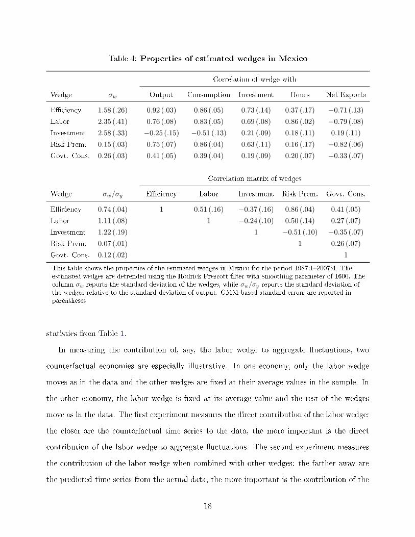
Consider, �rst, the properties of the estimated wedges. Tables 4 and 5 report some summary
statistics of the estimated wedges in Mexico and Canada respectively.7 Each table is divided
into two panels. The top panel reports the standard deviation of the estimated wedges and
the correlation of the wedges with each of the observable variables: output, consumption,
investment, hours, and net exports. The lower panel reports the standard deviation of the
wedges relative that of output and the correlation matrix of the estimated wedges.
Comparing the second column of the top panel of Table 4 with that of Table 5, we observe
that, except for the government consumption wedge, all wedges in Mexico are substantially
more volatile than in Canada: the e�ciency wedge by over 60 percent, the labor wedge by
over 30 percent, the investment wedge by over 80 percent, and the risk premium wedge by 50
percent. Note that these magnitudes are in line with the volatility of output, which is almost
50 percent higher in Mexico (Table 1). These numbers, on the other hand, are somewhat
di�erent when measured relative to the volatility of output (second column of the lower panel
of Tables 4 and 5). While the relative volatility of the e�ciency and investment wedges is
higher in Mexico, the relative volatility of the labor wedge is higher in Canada, and the relative
volatility of the risk premium wedge is similar in both countries.
Consider now the correlation of the wedges with the data. The upper panel of Table 4
shows that, in Mexico, output, consumption, investment, and hours worked are all positively
correlated with the e�ciency wedge, with the labor wedge, with the risk premium wedge,
and with the government consumption wedge. Output and consumption, however, are both
negatively correlated with the investment wedge. In other words, these correlations suggest
that downturns in Mexico are periods in which productivity is low, periods in which labor
decisions and intertemporal consumption choices are relatively more distorted, but are periods
7In computing these numbers, the estimated wedges were �rst HP-�ltered with a smoothing parameter of1600. GMM-based standard errors are reported in parentheses in these and all the tables that follow. Theoptimal weighting matrix is computed using the Newey-West estimator with a lag length equal to one fourthof the sample size.
16
in which investment decisions are relatively less distorted.
In Canada, on the other hand, the co-movements are somewhat di�erent. First, the invest-
ment wedge is positively correlated with output and consumption, meaning that investment
decisions are indeed relatively more distorted in downturns (upper panel of Table 5). Second,
the risk premium wedge is virtually uncorrelated with output, consumption, and investment,
but is negatively correlated with hours and net exports. Finally, and in contrast with Mex-
ico, the government consumption wedge is positively correlated with output. This �nding is
consistent with the observation that �scal policy is countercyclical in developed countries but
procyclical in developing countries (Kaminsky, Reinhart, and Vegh, 2005).8
The remainder of this section describes the contribution of the di�erent wedges, both
in isolation and in combination with other wedges, to aggregate �uctuations in Mexico and
Canada. Tables 6 and 7 display some summary statistics of the counterfactual economies with
di�erent active and inactive wedges. In reporting these results, I �rst added an exponential
trend equal to the sum of the estimated productivity and population growth rates to the
counterfactual time series, and next I HP-�ltered the resulting series. This transformation
replicates the transformation applied to the data.
The counterfactual experiments are divided into models with one active wedge (panel A),
models with two active wedges (panel B), and so on. The second and third columns provide a
measure of how well the di�erent models match output: the second column reports the relative
standard deviation of counterfactual output to actual output and the third column measures
the correlation between the two output series. If both of these numbers are close to one, the
model �ts output reasonably well. The last four columns report some summary statistic of
the counterfactual series: the volatility of the share of net exports on output, the volatility of
consumption and investment relative to that of output, and the correlation between output
and the share of net exports on output. The �rst row of these tables rewrites the summary
8The higher volatility of the risk premium wedge and its positive and signi�cant correlation with mosteconomic aggregates in Mexico but not in Canada is consistent with the �ndings in Neumeyer and Perri(2005) and Uribe and Yue (2006).
17
Table 4: Properties of estimated wedges in Mexico
Correlation of wedge with
Wedge σw Output Consumption Investment Hours Net Exports
This table shows the properties of the estimated wedges in Mexico for the period 1987:1�2007:4. Theestimated wedges are detrended using the Hodrick Prescott �lter with smoothing parameter of 1600. Thecolumn σw reports the standard deviation of the wedges, while σw/σy reports the standard deviation ofthe wedges relative to the standard deviation of output. GMM-based standard errors are reported inparentheses
statistics from Table 1.
In measuring the contribution of, say, the labor wedge to aggregate �uctuations, two
counterfactual economies are especially illustrative. In one economy, only the labor wedge
moves as in the data and the other wedges are �xed at their average values in the sample. In
the other economy, the labor wedge is �xed at its average value and the rest of the wedges
move as in the data. The �rst experiment measures the direct contribution of the labor wedge:
the closer are the counterfactual time series to the data, the more important is the direct
contribution of the labor wedge to aggregate �uctuations. The second experiment measures
the contribution of the labor wedge when combined with other wedges: the farther away are
the predicted time series from the actual data, the more important is the contribution of the
18
Table 5: Properties of estimated wedges in Canada
Correlation of wedge with
Wedge σw Output Consumption Investment Hours Net Exports
This table shows the properties of the estimated wedges in Canada for the period 1976:1�2007:4. Theestimated wedges are detrended using the Hodrick Prescott �lter with smoothing parameter of 1600. Thecolumn σw reports the standard deviation of the wedges, while σw/σy reports the standard deviation ofthe wedges relative to the standard deviation of output. GMM-based standard errors are reported inparentheses
labor wedge, when combined with other wedges, to aggregate �uctuations.9
Consider, �rst, counterfactual economies with only one active wedge. These experiments,
displayed in panel A of Tables 6 and 7, suggest that only the e�ciency and labor wedges could
account, by themselves, for an important fraction of output �uctuations in both countries.
The models with just the e�ciency wedge and just the labor wedge, however, completely
miss the volatility of consumption and investment relative to that of output, and the negative
correlation between output and the share of net exports on output in Mexico. Likewise,
in Canada, the models with only e�ciency wedges and only labor wedges predict a large
positive correlation between output and the share of net exports in output, and understate
9Because the government consumption wedge plays a negligible role in both countries, panels B and C ofTables 6 and 7 do not include experiments with the government consumption wedge.
19
the volatility of investment relative to that of output. These models, on the other hand, are
consistent with the smaller volatility of consumption relative to that of output in Canada.
The investment, risk premium, and government consumption wedges, by themselves, can-
not explain aggregate �uctuations in either country. In Mexico, the economy with just the
investment wedge accounts for only 10 percent of output volatility, grossly overstates the
volatility of consumption and investment relative to that of output, and misses the negative
correlation between output and the share of net exports on output. In the economy with
just the risk premium wedge, predicted and actual output are negatively correlated, and the
correlation of output with the share of net exports on output is extremely large. Finally,
the economy with just the government consumption wedge accounts for only 4 percent of
the output volatility and misses the volatility of the share of net exports on output and the
correlation between output and the share of net exports on output. Likewise, in Canada,
the model with just the investment wedge explains only 16 percent of the volatility of output
and also completely overstates the volatility of consumption and investment relative to that
of output. In the model with just the risk premium wedge, predicted output is negatively
correlated with actual output, consumption is more volatile than output, and the correlation
of output and the share of net exports on ouput is almost one. Finally, the model with just
the government consumption wedge accounts for only 7 percent of the volatility of output.
Consider now counterfactual economies with all wedges but one. Panel D of Table 6
suggests that three wedges are essential to understand business cycles in Mexico: the e�ciency
wedge, the labor wedge, and the risk premium wedge. Eliminating any of these wedges causes
the model to miss the data in some dimension. In the model with no e�ciency wedges,
predicted output is 54 percent less volatile than actual output and their correlation is just
0.53, investment is over eight times more volatile than output, and the correlation between
output and the share of net exports on output is only -0.17. In the model with no labor wedges,
predicted output is 43 percent less volatile than actual output and their correlation is only
0.41, the volatility of consumption and investment relative to that of output is overstated, and
20
Table 6: Contribution of the wedges to aggregate �uctuations in Mexico
E�., Lab., R. Pr. 0.93 (.02) 0.99 (.05) 2.15 (.38) 1.53 (.07) 4.66 (.19) −0.66 (.05)
E�., Inv., R. Pr. 0.55 (.08) 0.36 (.07) 2.99 (.07) 2.16 (.27) 7.45 (1.4) 0.02 (.13)
Lab., Inv., R. Pr. 0.45 (.07) 0.487 (.10) 2.16 (.56) 1.63 (.21) 8.88 (1.7) −0.12 (.14)
D. Economies with four active wedges
All but E�ciency 0.46 (.07) 0.53 (.09) 2.15 (.60) 1.58 (.21) 8.74 (1.7) −0.17 (.14)
All but Labor 0.57 (.09) 0.41 (.07) 3.02 (.70) 2.15 (.27) 7.37 (1.4) −0.02 (.13)
All but Investment 0.95 (.02) 1.00 (.00) 2.18 (.39) 1.51 (.07) 4.63 (.18) −0.67 (.04)
All but Risk Prem. 1.62 (.03) 0.98 (.03) 2.19 (.35) 0.47 (.06) 2.00 (.20) 0.92 (.02)
All but Government 0.97 (.00) 1.00 (.00) 1.61 (.43) 1.30 (.05) 4.59 (.42) −0.79 (.12)
This table reports the contribution of the wedges to aggregate �uctuations in Mexico. For consistency whencomparing the models with the data, the counterfactual series were exponentially retrended using the averagepopulation and output growth rates, and then detrended using the Hodrick Prescott �lter with a smoothingparameter of 1600. The statistic σ(x) measures the standard deviation of the series x, while ρ(x, y) measuresthe correlation coe�cient between the series x and y. Counterfactual time series are denoted with asuperscript o. The variable y denotes output; m, net exports; and c, private consumption. GMM-basedstandard errors are reported in parentheses.
21
Table 7: Contribution of the wedges to aggregate �uctuations in Canada
E�., Lab., R. Pr. 0.96 (.02) 0.98 (.00) 0.86 (.06) 0.79 (.04) 1.69 (.18) 0.66 (.07)
E�., Inv., R. Pr. 1.12 (.27) 0.57 (.09) 1.89 (.20) 0.82 (.13) 3.93 (.85) 0.51 (.14)
Lab., Inv., R. Pr. 0.92 (.16) 0.33 (.19) 1.50 (.13) 1.03 (.10) 4.71 (.69) 0.20 (.22)
D. Economies with four active wedges
All but E�ciency 0.93 (.15) 0.36 (.19) 1.54 (.13) 1.03 (.05) 4.74 (.66) 0.28 (.20)
All but Labor 1.16 (.28) 0.59 (.09) 1.80 (.19) 0.56 (.08) 3.94 (.81) 0.57 (.13)
All but Investment 1.00 (.02) 0.99 (.00) 1.10 (.09) 0.65 (.06) 1.56 (.15) 0.70 (.07)
All but Risk Prem. 1.08 (.05) 0.95 (.02) 0.56 (.04) 0.66 (.03) 3.94 (.20) 0.22 (.09)
All but Government 0.96 (.01) 1.00 (.00) 0.93 (.10) 0.98 (.06) 4.67 (.25) −0.26 (.24)
This table reports the contribution of the wedges to aggregate �uctuations in Canada. For consistency whencomparing the models with the data, the counterfactual series were exponentially retrended using the averagepopulation and output growth rates, and then detrended using the Hodrick Prescott �lter with a smoothingparameter of 1600. The statistic σ(x) measures the standard deviation of the series x, while ρ(x, y) measuresthe correlation coe�cient between the series x and y. Counterfactual time series are denoted with asuperscript o. The variable y denotes output; m, net exports; and c, private consumption. GMM-basedstandard errors are reported in parentheses.
22
the correlation of output with the share of net exports on output is zero. Finally, in the model
with no risk premium wedges, predicted output is 62 percent more volatile than actual output,
consumption is substantially less volatile than output, the volatility of investment relative to
that of output is understated, and the share of net exports on output is highly procyclical. The
investment and government consumption wedges, on the other hand, can be eliminated from
the model without severely a�ecting the ability of the model to match the data. Interestingly,
the investment wedge does not even contribute to the volatility of aggregate investment: the
model with no investment wedges matches the volatility of investment relative to that of
output remarkably well.
Panel D of table 7, on the other hand, suggest that two wedges are essential to understand
business cycles in Canada: the e�ciency wedge and the labor wedge. There is, however, some
role for the investment wedge and a small role for the risk premium wedge. The model with
no investment wedges predicts a substantially lower volatility of investment compared to that
in the data and a highly procyclical share of net exports on output; and the model with no
risk premium wedges understate the volatility of the share of net exports on output.
Overall, these �ndings suggest that business cycles in Mexico can be explained by the
combined e�ect of the e�ciency wedge, the labor wedge, and the risk premium wedge. More-
over, the risk premium wedge is the key to understand the excess volatility of consumption
over output and the highly countercyclical share of net exports on output. Business cycles
in Canada, on the other hand, can be explained reasonably well by the combined e�ect of
the e�ciency wedge and the labor wedge. The investment wedge contributes somewhat to
the behavior of investment and net exports, and the risk premium wedge has, if anything, a
secondary role.
Two Recession Episodes
Now I apply the decomposition methodology to study two recession episodes: the 1995 Mex-
ican `Tequila' crisis and the 1983 Canadian recession. In summary, the results of this section
23
are consistent with the �ndings in the previous section with two exceptions: the investment
wedge contributes to the recovery of output and labor in Canada, and the worsening in the
risk premium wedge prevented an even larger drop in output and labor in Canada.
The 1995 Mexican Crisis
The upper panel of Figure 1 shows output and the estimated wedges in the 1995 Mexican
crisis. The series have been normalized to equal 100 at the beginning of the episode and the
units of the risk premium wedge are shown on the right vertical axis. Output falls 12 percent
in two quarters and remains below trend until 2000. The e�ciency, labor, and risk premium
wedges deteriorate throughout the recession, although by 1998, the labor wedge fully recovers.
The investment wedge, on the other hand, improves substantially throughout the episode,
suggesting that investment decisions were, in fact, relatively less distorted during the Mexican
crisis. The solid blue lines in Figure 2 display Mexican data. Labor (hours) is normalized to
equal 100 at the beginning of the recession; investment and net exports are normalized by the
initial level of output, and are shown in percentage points. Labor initially drops 3 percent
but soon recovers, and by 1998 it is over 4 percent above its initial value. Investment drops
abruptly and co-moves closely with output. Finally, net exports move sharply from a de�cit
of 4 percent to a surplus of 4 percent and remain in surplus until 1998.
The contribution of the wedges to the Mexican crisis is shown in Figures 2 and 3. These
�gures report counterfactual experiments in which the active wedges are set to their estimated
values and the inactive wedges are set at their values at the beginning of the crisis. Consider,
�rst, the direct contribution of the e�ciency wedge. The model with just the e�ciency wedge,
shown in the upper panel of Figure 2, matches the evolution of output and labor remarkably
well until 1997. Thereafter, the model predicts a somewhat slower recovery compared with that
in the data. The model also misses the evolution of investment and net exports throughout the
episode: predicted investment declines by a small amount and predicted net exports actually
Figure 1: Output and four wedges in two recessions. (Data normalized to equal 100before the recession; risk premium wedge is on left axis.)
25
Consider next the labor wedge. The model with just the labor wedge, also shown in the
upper panel of Figure 2, predicts a fall in output of about one third of the fall in the data and
a fall in labor larger than that in the data. This model captures the recovery and most ups
and downs in output and labor, but also fails to match investment and net exports.
The models with just the investment wedge and with just the risk premium wedge, shown
in the lower panel of Figure 2, cannot explain the crisis. The model with just the investment
wedge completely misses the data: it predicts a steady increase in output and labor, and a
small initial decline in investment followed by a strong increase since mid-1995. The model
with just the risk premium wedge predicts an increase in output and labor, a small decline in
investment, and a large increase in net exports. Note, however, that the risk premium wedge
is the only wedge that, by itself, drives an increase in net exports.
Consider now economies with all wedges but one. In the model with no e�ciency wedge,
displayed in the upper panel of Figure 3, predicted output actually increases and predicted
labor �uctuates until mid-1996 but matches the data closely thereafter. The model predicts
an initial fall in investment of about two thirds of the fall in the data and matches its recovery
almost perfectly thereafter. In addition, the model overstates the initial increase in net exports
but matches that series closely after 1996. In other words, the e�ciency wedge contributes
substantially to the behavior of output, to the initial decline in labor, and somewhat to the
drop in investment. Note, however, that because this model predicts a recovery similar to that
in the data (saving the level of output), it has to be that other wedges are mainly responsible
for the recovery after 1996.
Consider now the model with no labor wedge, also shown in the upper panel of Figure 3. In
this model, predicted output drops about half of the drop in the data and recovers faster that
actual output does; predicted labor increases throughout the episode; predicted investment
matches the data almost perfectly; and predicted net exports increase substantially more than
actual net exports do. That is, the labor wedge contributes substantially to the behavior of
output, labor, and net exports; and to the recovery since 1996.
26
1995 1996 1997 1998
85
90
95
100
105
110 Output
1995 1996 1997 199810
15
20
25
30
35 Investment
1995 1996 1997 1998
90
95
100
105
110 Labor
1995 1996 1997 1998
−10
−5
0
5
10
Net Exports
Model with Efficiency Wedge Model with Labor Wedge Data
Mexico
1995 1996 1997 1998
85
90
95
100
105
110 Output
1995 1996 1997 199810
15
20
25
30
35 Investment
1995 1996 1997 1998
90
95
100
105
110
Labor
1995 1996 1997 1998
−10
−5
0
5
10
Net Exports
Model with Investment Wedge Model with Risk−Premium Wedge Data
MexicoMexico
Figure 2: Data and counterfactual models with one wedge.
27
1995 1996 1997 1998
85
90
95
100
105
110 Output
1995 1996 1997 199810
15
20
25
30
35 Investment
1995 1996 1997 1998
90
95
100
105
110
Labor
1995 1996 1997 1998
−10
−5
0
5
10
Net Exports
Model with No Efficiency Wedge Model with No Labor Wedge Data
Mexico
1995 1996 1997 1998
85
90
95
100
105
110 Output
1995 1996 1997 199810
15
20
25
30
35 Investment
1995 1996 1997 1998
90
95
100
105
110
Labor
1995 1996 1997 1998
−10
−5
0
5
10
Net Exports
Model with No Investment Wedge Model with No Risk−Premium Wedge Data
Mexico
Figure 3: Data and counterfactual models with four wedges.
28
Now consider the model with no risk premium wedge, shown in the lower panel of Figure
3. This model predicts a drop in output and labor substantially larger that those in the data;
a drop in investment about half of the drop in the data, and a large drop in net exports. In
addition, this model does not match the behavior of consumption either (not shown in these
�gures). In other words, the risk premium wedge contributes substantially to the Mexican
crisis. While its contribution to the behavior of output and labor is important, the most
important role of the risk premium wedge is in the behavior of net exports: without that
wedge, the model is unable to explain the large increase in net exports and the behavior of
consumption.10
Consider, �nally, the model with no investment wedges. The plots in the lower panel
of Figure 3 show that shutting down the investment wedge does not a�ect the ability of the
model to match output, labor, and net exports. Because the model with no investment wedges
cannot explain the full drop in investment and its recovery, I conclude that, if anything, the
investment wedge only contributes to the behavior of investment in the Mexican crisis.
Summarizing, these �ndings are consistent with those of the previous section and suggest
that the e�ciency wedge, the labor wedge, and the risk premium wedge account for most of
the aggregate behavior in the Mexican 1995 crisis. Moreover, among all wedges, only the risk
premium wedge is able to account for the behavior of net exports in the Mexican crisis.
The 1983 Canadian Recession
Now I apply the decomposition methodology to the 1983 Canadian recession. The lower panel
of Figure 1 displays output and the estimated wedges in that episode. Output drops by 9
percent at the trough of the recession. There is a small decline in the e�ciency wedge, which
10The large drop in output and labor in the model with no risk premium wedges is likely to disappear if Ichange the period utility function and adopt the preferences proposed by Greenwood, Hercowitz, and Hu�man(1988). With these preferences, changes in interest rates do not have a wealth e�ect on labor supply; therefore,the worsening in the risk premium wedge need not imply an increase in hours and, therefore, in output. Thesepreferences, however, are inconsistent with a balanced growth path unless one assumes that the disutility ofwork increases at the growth rate of technology, an undesirable feature in preferences.
29
returns to trend by 1984. The labor wedge worsens substantially and tracks output closely.
The investment wedge also follows output closely until 1984; afterwards, output recovers but
the investment wedge does not. The risk premium wedge, on the other hand, remains �at until
mid-1983; then it worsens slightly but recovers by the second quarter of 1984. The solid blue
lines in Figure 4 displays Canadian data. Investment and labor co-move closely with output,
although investment recovers more slowly than output does. Net exports, on the other hand,
increase from 0 to over 4 percent and remain in surplus for several years.
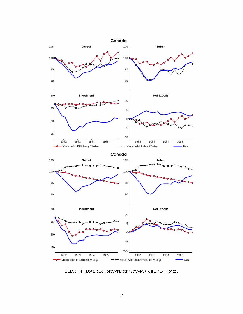
Consider �rst counterfactual economies with only one active wedge. The upper panel of
Figure 4 shows the prediction of the models with just the e�ciency wedge and just the labor
wedge. The model with the e�ciency wedge alone misses the drop in output, labor, and
investment, and predicts a small decline in net exports. The model with just the labor wedge
matches hours remarkably well and accounts for about two thirds of the drop in output. This
model, however, misses investment and net exports. The model with just the investment
wedge, shown in the lower panel of Figure 4, completely misses output and labor, but matches
investment and net exports reasonably well. Finally, the model with just the risk premium
wedge predicts an increase in output, an increase in labor, misses the behavior of investment,
but matches net exports well.
Consider now models with all wedges but one. The top panel of Figure 5 displays the
predictions of the models with no e�ciency wedge and with no labor wedge. The lower
panel of that �gure shows the models with no investment wedge and no risk premium wedge.
The model with no e�ciency wedge matches labor, investment, and net exports closely, but
predicts a somewhat smaller decline and slower recovery in output compared with those in
the data. The model with no labor wedge completely misses output and labor, matches
investment closely, and overstates the increase in net exports. The model with no investment
wedge matches output and labor closely, although it predicts a somewhat faster recovery than
that in the data. This model, on the other hand, misses the behavior of investment and net
exports. Consider, �nally, the model with no risk premium wedge. This model misses net
30
1982 1983 1984 1985
90
95
100
105 Output
1982 1983 1984 1985
15
20
25
30 Investment
1982 1983 1984 1985
90
95
100
105 Labor
1982 1983 1984 1985
−10
−5
0
5
10
Net Exports
Model with Efficiency Wedge Model with Labor Wedge Data
Canada
1982 1983 1984 1985
90
95
100
105 Output
1982 1983 1984 1985
15
20
25
30 Investment
1982 1983 1984 1985
90
95
100
105 Labor
1982 1983 1984 1985
−10
−5
0
5
10
Net Exports
Model with Investment Wedge Model with Risk−Premium Wedge Data
CanadaCanada
Figure 4: Data and counterfactual models with one wedge.
31
1982 1983 1984 1985
90
95
100
105 Output
1982 1983 1984 1985
15
20
25
30 Investment
1982 1983 1984 1985
90
95
100
105 Labor
1982 1983 1984 1985
−10
−5
0
5
10
Net Exports
Model with No Efficiency Wedge Model with No Labor Wedge Data
Canada
1982 1983 1984 1985
90
95
100
105 Output
1982 1983 1984 1985
15
20
25
30 Investment
1982 1983 1984 1985
90
95
100
105 Labor
1982 1983 1984 1985
−10
−5
0
5
10
Net Exports
Model with No Investment Wedge Model with No Risk−Premium Wedge Data
Canada
Figure 5: Data and counterfactual models with four wedges.
32
exports and predicts a larger drop in output and labor, and a somewhat smaller decline in
investment compared with those in the data.
Overall, these �ndings suggest that most of the drop in output and labor is due to the
labor wedge; the e�ciency wedge has a somewhat smaller role; the investment wedge accounts
for the behavior of investment and somewhat for the recovery; and the slight worsening in
the risk premium wedge in 1983-1984 acted to avoid a larger drop in output and labor�see,
however, the discussion in footnote 10.
5 Discussion and Conclusion
In this paper I have decomposed �uctuations in Mexico and in Canada in terms of reduced form
shocks that drive a wedge between certain marginal rates of substitution and marginal rates
of transformation relative to a prototype frictionless economy. I have found that the business
cycle and the 1995 crisis in Mexico can be explained, to a large extent, by the combined e�ect
of the e�ciency wedge, the labor wedge, and the risk premium wedge. And what is most
important, the risk premium wedge accounts for the large increase in net exports in the 1995
crisis, the excess volatility of consumption over output, and the highly countercyclical share
of net exports on output in Mexico. Business cycles in Canada, on the other hand, are mostly
driven by �uctuations in the e�ciency wedge and in the labor wedge.
Investment wedges do not contribute at all to �uctuations in Mexico, not even to �uc-
tuations in aggregate investment. Moreover, the investment wedge is countercyclical and
improved substantially during the 1995 crisis. In other words, investment decisions in Mexico
are less distorted in downturns and more distorted in booms relative to a frictionless economy.
In Canada, on the other hand, the investment wedge is procyclical and contributes somewhat
to the behavior of aggregate investment and net exports.
If Mexico is, indeed, a representative emerging country and Canada a representative devel-
oped small open country, these �ndings have implications for model development. Successful
33
models of emerging market �uctuations should generate the type of wedges that we observe in
the data, and these wedges should account, quantitatively, for aggregate �uctuations. Thus,
we need to understand what type of primitive shocks and transmission mechanisms drive �uc-
tuations in the risk premium wedge, in the e�ciency wedge, and in the labor wedge. Moreover,
because a successful model should also induce countercyclical investment wedges, the trans-
mission mechanisms and the spillovers from the primitive shocks to the wedges should be
strong enough to mitigate the countercyclical e�ect of the investment wedge.
There are models consistent with some of these requirements. The working capital require-
ment on labor demand stressed by Neumeyer and Perri (2005), Uribe and Yue (2006), and
Mendoza (2008); and on imported inputs, stressed by Mendoza (2008), translates shocks to the
interest rate into labor and e�ciency wedges respectively. The problem is that in those models
�uctuations in interest rates are exogenous and, therefore, the issue of why the risk premium
wedge in Mexico is di�erent from that in Canada is left unexplained. The paper by Mendoza,
however, also includes a collateral constraint that, when binding, induces an endogenous risk
premium wedge that ampli�es the labor and e�ciency wedges induced by the working capital
constraints. Moreover, as Chari, Kehoe, and McGrattan (2005) show, a tightening in the
collateral constraint could manifest itself as an improvement in the investment wedge, which
is, in fact, observed in the Mexican crisis. Still, in periods in which the collateral constraint
is slack, Mendoza's model reduces to a model with exogenous �uctuations in interest rates.
These �uctuations need to be understood. A step in that direction are the endogenous default
models of Aguiar and Gopinath (2006) and Arellano (2008). These models, however, are still
at an early stage of development and are either endowment or labor only economies; it is not
clear if full-blown versions of these models will be consistent with all the business cycles facts.
This paper can be extended in a number of directions. The most obvious is to apply
the methodology to other emerging countries and check whether the results are robust. The
problem here is with the length of the time series and the large number of parameters that
need to be estimated. Because most emerging countries do not have su�ciently long time
34
series, the estimates of the 44 parameters will likely be inaccurate. Note, however, that the
similarity of the business cycle within the group of emerging countries suggests that the most
important results will remain intact.
A second possibility is to extend the framework along the lines of Aguiar and Gopinath
(2007). In that paper, they argue that the most important di�erence between emerging and
developed countries lies in the persistence of the total productivity shocks they face. Emerging
countries, they claim, are mostly subject to trend shocks, while developed countries are mostly
subject to temporary shocks. It is possible to extend the prototype economy along these lines
by posing two types of e�ciency wedges, one temporary and one permanent. With this
extension we could study whether the di�erences between emerging and developed countries
are due to the di�erent type of productivity shocks they face, to di�erent risk premium wedges,
or to both. This extension, however, could be di�cult to implement because the number of
parameters to estimate increases by 50 percent, making the maximization of the likelihood
function�already challenging in the present formulation�substantially more di�cult.11
11The number of parameters to estimate increases to 63: 6 means, 36 coe�cients in the matrix on laggedvalues, and 21 coe�cients in the covariance matrix.
35
Appendix A Sources and Construction of the Data
Mexico
All series, except population data, are from Instituto Nacional de Estadísticas y Geografía�http://dgcnesyp.inegi.gob.mx/cgi-win/bdieintsi.exe. Data are quarterly series on output, in-vestment, labor, net exports, and government consumption for the period 1987:1�2007:4.Output is �gross domestic product�, investment is �gross �xed capital formation� plus �changein inventories�, net exports are �exports of goods and services� minus �imports of goods andservices�, and government consumption is �government consumption expenditures�, all at 1993prices. The data were seasonally adjusted using the Census Bureau's X-12 ARIMA program.
Labor is (Average hours worked)×(Employment)/(Available Hours). Data on Averagehours worked are from the Encuesta Industrial Mensual. For the period 1987:M01�1995:M12,I use the survey with 129 activity classes; for the period 1994:M01�2007:M12, the survey with205 activity classes. Overlapping periods are averaged, and quarterly �gures are averages ofmonthly data. Employment is (1-unemployment rate)×(Rate of activity of population over 14years of age)×(Total population over 14 years of age). For the period 1987:M01�2000:M04,unemployment data are from the Encuesta Nacional de Empleo Urbano (ENEU). For theperiod 2000:M04-2007:M12, unemployment data are from the Encuesta Nacional de Ocupacióny Empleo (ENOE). The data on the Rate of activity of population over 14 years of age arein quarterly frequency. For the period 1987:01�2004:04, data is from ENEU: �Economicallyactive population over 12 years of age�. For the period 2005:01�2007:04, data is from ENOE:�Economically active population over 14 years of age�. To match the levels of the series, Iadded a 1% to the series before 2005:01. This procedure roughly transforms the �rst series toeconomically active population over 14 years of age. Data on Total population over 14 yearsof age are from the World Development Indicators. Quarterly �gures are interpolated fromannual data. Lastly, Available hours is (Total population over 14 years of age)×100, assuming100 hours per week for work or leisure.
Canada
National accounts data are from OECD Quarterly National Accounts Statistics. Seasonallyadjusted series at current prices (CAN.CARSA.S1 series) are de�ated using the GDP de�atorseries (CAN.DOBSA2000). Labor data is from LABORSTA Labor Statistics Database. Laboris constructed as in Mexico, except that Employment is directly observed. Average hoursworked is from series �B6 Hours of work per week in manufacturing�. I use the series �hourspaid for wage earners, total men and women�; missing observations are �lled using �hours paidfor employees, total men and women�. Employment is from series �B1 Employment, generallevel�. The employment series has a structural break in January 1995 due to a methodologicalchange. The break in the trend was adjusted using an extended Hodrick-Prescott �lter thatallows for structural breaks (Schlicht, forthcoming). Labor data were seasonally adjusted usingthe Census Bureau's X-12 ARIMA program, and quarterly �gures are averages over monthlydata. Population data is from the World Development Indicators.
The model is stationary in terms of the variables xt = xt/(1 + γ)t for any xt except for laborand the rental rate of capital.12 Let xt be the steady state value of any variable xt. Toapproximate the equilibrium, the model is �rst log-linearized around the steady state andthen written in the state space form
Xt+1 = M (θ)Xt + νt+1 (B.1)
Yt = N (θ)Xt, (B.2)
Here (B.1) is the state transition equation; (B.2) is the observation equation; Xt and Yt arethe state vector and observation vector, both in terms of deviations from the steady state andgiven by
Xt =[log(kt/k
), log
(bt/b
), log
(At/A
), τlt − τl, τxt − τx, log
(Zt/Z
), log (gt/g)
]Yt =
[log (yt/y) , log (xt/x) , log
(lt/l), m− m, log (gt/g)
];
the noise process in (B.1) is given by νt+1 = [0, 0, εt+1]′, where εt+1 is the innovation of the
stochastic process (11); and the matrices M(θ) and N (θ) are nonlinear functions of theparameters θ = {s, P, V }. The remaining parameters of the model (σ, ρ, and so on) are held�xed throughout the estimation.
I �rst construct the empirical analogs of yt, xt, lt, mt, and gt using data on output,investment, labor, net exports, and government consumption. This is done by exponentiallydetrending the data using the average growth rate of the population and output. (Hoursworked are only detrended using the population growth rate.)
Given a guess θ, I solve for the log-linearized policy functions M (θ) and N (θ), and con-struct a time series Yt using the transformed data and the steady state values. The likelihoodfunction is then evaluated using the Kalman �lter on the system (B.1�B.2). To maximize thelog-likelihood function, I follow Chari, Kehoe, and McGrattan (2007), and apply the followingtransformations: to induce positive de�niteness of V , I estimate the lower triangular Choleskydecomposition of V ; to induce stationarity, I add a penalty term of 5× 10⁵ max (λ− 0.995, 0)2
to the likelihood function, where λ is the eigenvalue of P with the largest absolute value.The maximization step is di�cult: the log-likelihood is a nonlinear function of 44 param-
eters. I �rst use a simulated annealing algorithm (Kirkpatrick, Gelatt, and Vecchi, 1983) toobtain an approximation to the global optimum. Next I use the estimate from the annealingstep to initialize a local search algorithm: a Quasi-Newton algorithm, a Nelder-Mead simplexalgorithm, or both. Next I perturb the estimate from the previous step and use it to restartthe local search algorithm. After repeating this cycle several times, I use the best estimateobtained so far to restart the simulated annealing algorithm, and repeat the process until nofurther improvements in the log-likelihood can be obtained.
12In the case of capital and debt, let kt = k(st−1)/(1 + γ)t and bt = k(st−1)/(1 + γ)t.
37
References
Aguiar, M. and G. Gopinath (2006): �Defaultable debt, interest rates and the currentaccount,� Journal of International Economics, 69, 64�83.
��� (2007): �Emerging Market Business Cycles: The Cycle Is the Trend,� Journal ofPolitical Economy, 115, 69�102.
Anderson, B. D. O. and J. B. Moore (2005): Optimal Filtering (Dover Books on Engi-neering), Dover Publications.
Arellano, C. (2008): �Default Risk and Income Fluctuations in Emerging Economies,�American Economic Review, 98, 690�712.
Bernanke, B. and M. Gertler (1989): �Agency Costs, Net Worth, and Business Fluctu-ations,� American Economic Review, 79, 14�31.
Bernanke, B. S., M. Gertler, and S. Gilchrist (1999): �The Financial Accelerator ina Quantitative Business Cycle Framework,� in Handbook of Macroeconomics, ed. by J. B.Taylor and M. Woodford, Elsevier, vol. 1 of Handbook of Macroeconomics, chap. 21, 1341�1393.
Bordo, M. D., C. J. Erceg, and C. L. Evans (2000): �Money, Sticky Wages, and theGreat Depression,� American Economic Review, 90, 1447�1463.
Carlstrom, C. T. and T. S. Fuerst (1997): �Agency Costs, Net Worth, and BusinessFluctuations: A Computable General Equilibrium Analysis,� American Economic Review,87, 893�910.
Chari, V. V., P. J. Kehoe, and E. R. McGrattan (2002): �Accounting for the GreatDepression,� American Economic Review, 92, 22�27.
��� (2005): �Sudden Stops and Output Drops,� American Economic Review, 95, 381�387.
Christiano, L. J., C. Gust, and J. Roldós (2004): �Monetary Policy in a FinancialCrisis,� Journal of Economic Theory, 119, 64�103.
Cole, H. L. and L. E. Ohanian (2004): �New Deal Policies and the Persistence of theGreat Depression: A General Equilibrium Analysis,� Journal of Political Economy, 112,779�816.
Greenwood, J., Z. Hercowitz, and G. W. Huffman (1988): �Investment, CapacityUtilization, and the Real Business Cycle,� American Economic Review, 78, 402�17.
Hall, R. E. (1997): �Macroeconomic Fluctuations and the Allocation of Time,� Journal ofLabor Economics, 15, S223�S250.
38
Hamilton, J. D. (1994): Time Series Analysis, Princeton University Press.
Kaminsky, G. L., C. M. Reinhart, and C. A. Vegh (2005): �When It Rains, It Pours:Procyclical Capital Flows and Macroeconomic Policies,� NBER Macroeconomics Annual,11�82.
Kirkpatrick, S., C. D. Gelatt, and M. P. Vecchi (1983): �Optimization by SimulatedAnnealing,� Science, 220, 671�680.
Kiyotaki, N. and J. Moore (1997): �Credit Cycles,� Journal of Political Economy, 105,211�48.
Mendoza, E. G. (2008): �Sudden Stops, Financial Crises and Leverage: A Fisherian De�a-tion of Tobin's Q,� .
Mulligan, C. B. (2002): �A Century of Labor-Leisure Distortions,� Working Paper 8774,National Bureau of Economic Research.
Neumeyer, P. A. and F. Perri (2005): �Business Cycles in Emerging Economies: TheRole of Interest Rates,� Journal of Monetary Economics, 52, 345�380.
Parkin, M. (1988): �A Method for Determining Whether Parameters in Aggregative ModelsAre Structural,� Carnegie-Rochester Conference Series on Public Policy, 29, 215�252.
Reinhart, C. M., K. S. Rogoff, and M. A. Savastano (2003): �Debt Intolerance,�Brookings Papers on Economic Activity, 34, 1�74.
Rotemberg, J. J. and M. Woodford (1999): �The Cyclical Behavior of Prices and Costs,�in Handbook of Macroeconomics, ed. by J. B. Taylor and M. Woodford.
Schlicht, E. (forthcoming): �Trend Extraction From Time Series With Structural Breaksand Missing Observations,� Journal of the Japan Statistical Association.
Schmitt-Grohé, S. and M. Uribe (2003): �Closing Small Open Economy Models,� Journalof International Economics, 61, 163�185.
Shimer, R. (2009): �Convergence in Macroeconomics: The Labor Wedge,� American Eco-nomic Journal: Macroeconomics, 1, 280�97.
Uribe, M. and V. Z. Yue (2006): �Country Spreads and Emerging Countries: Who DrivesWhom?� Journal of International Economics, 69, 6�36.