Emerging Technology in Optimization

Computational Mechanics Laboratory

The University of Michigan, Department of Mechanical Engineering

Emerging Technologyin Optimization

An Image Based Approach for CAE

Noboru Kikuchi

OptiCon’98



Major Collaborators

Alejandro Diaz

Michigan State University

Scott Hollister

University of Michigan

and

Keizo Ishii

QUINT Corporation



Graduate Students in CMLcurrent

Emilio SilvaShinji Nishiwaki & Susumu Ejima

J.H. YooBing-Chung Chen

Daichi FujiiMinako Sekiguchi



CAE at Present

An Introduction to Image Based CAE



Current Approach in CAE

l Parametric (Geometry Based) CAD / CAE– Standard CAD Software is based on computational

geometry by using parametric spline representationto define shape of a structure/domain

– All of the existing CAD software are geometrybased : Pro-E, UNIGRAPHICS, I-DEAS,CATIA, .....

– In FEA, automatic mesh generation methods arealso based on parametric representation ofgeometry



Lots of Sophisticationand

Big Success (2D,3D?)

Realization of importance andprofitability of Parametric

Geometry Based CAD and CAE



Industry Standard in CAD

l Automotive Industry

– UNIGRAPHICS in GM– I-DEAS in FORD– CATIA in CHRYSLER

l Leading companies have given up In-House CAD/CAE software

Paradigm Shift in 90s



CAD/CAE AcceptanceNot Yet

l 2D CAD is widely accepted, but 3DCAD is too sophisticated for majority ofdesigners and manufacturers

l CAE becomes an accepted tool forsingle disciplinary analysis, but notsufficient to create new value exceptfew areas ( crash, forming, etc )



MCAE+FCAE=CAE

l MCAE(Mechanical CAE)l FCAE(Fluid CAE)

l Two separated CAE, Two separatedPreprocessing Software, Two separatedCAE analysis specialists …..Difficulty ofIntegration for Design and Manufacturing



Trend in (M)CAE

l Major Software Houses– MSC/NASTRAN,PATRAN,ABAQUS

(US,Europe,Japan)– ESI/PAMCRASH,PAMSTAMP,COMPOSIC

(Europe,Japan,US)

– Others : Swanson/ANSYS, LS/DYNA, ALGOR,…..MDI/ADAMS,

Consolidation

LinearNonlinearImpact(Multi-Body)Design Optimization



Two Paths for Survival

l Total Consolidated MCAE/FCAE– Analysis(Linear,Nonlinear,Impact,Multi-body),

Design Optimization, Simulation ofManufacturing Processes : Total CAE

– ESI is a typical example : European’s Approach– MSC may follow : US for survival

l Integration with (Imbedding to) CAD– CAD software absorb linear CAE for Design

– MCAE is a part of major CAD software



CAD Imbedded MCAE

l CAD absorbs CAE softwarel Simulation of Design Feasibility

– Based on only Linear Analysis– users are Designers rather than Analysts– Less Accuracy but user oriented– possibly Design Optimization capability–

l Short Turn Around TimeDESIGN ORIENTED



Effort in MCAE

l For Shortening of Turn Around Time bySimplifying FE Modeling Methods

– CAD Linked Automatic Mesh Generation– Adaptive FE Methods (h and p elements)

– Meshless FE Methods (ANALYSIS)

l Integration with Design Optimization– Design Sensitivity Analysis– Size,Shape, and Topology Optimization



Importance

l Shortening of Modeling Timel Integration of MCAE and FCAE for

– Design and Simulation of Manufacturing Process

– Automatic Mesh Generation ? How?

PARADIGM CHANGE !



Image Based CAE

Originated From/Based OnOPTISHAPE

Topology Optimization



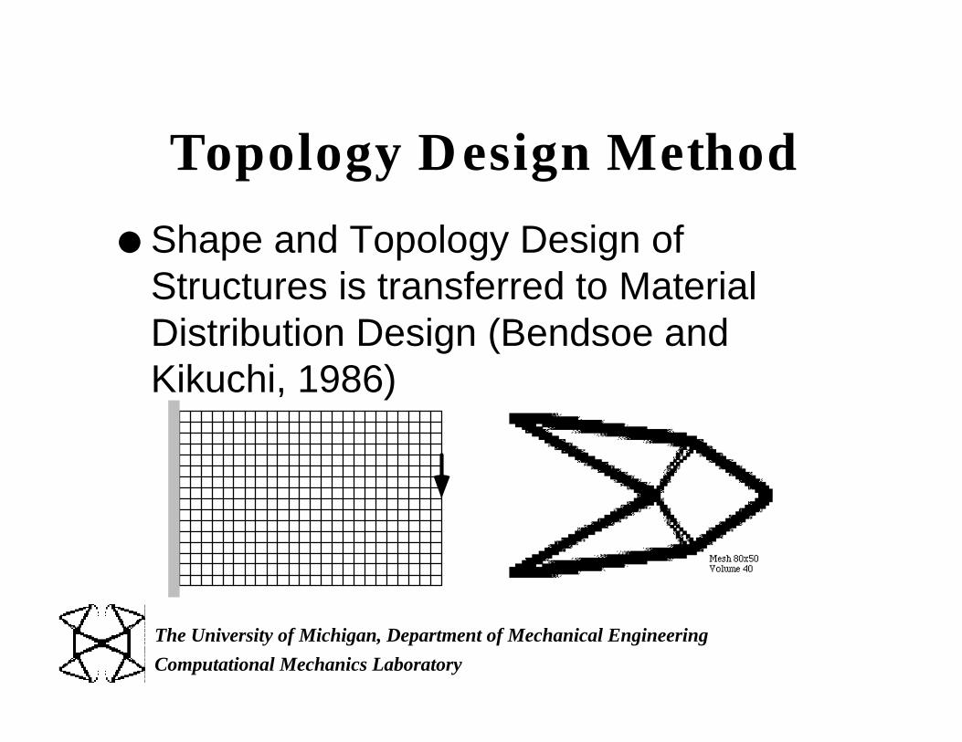
Topology Design Method

l Shape and Topology Design ofStructures is transferred to MaterialDistribution Design (Bendsoe andKikuchi, 1986)



TDM : 3D Shaping

Truly Three-dimensionalshaping of a structure foroptimum

Without parametric shapedefinition by splines



Closely Related to Rapid Prototype

Layer by Layer OperationLink with CAD for pixel operation

Utility of STL (SLC ) file



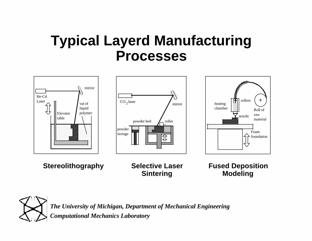
Typical Layerd ManufacturingProcesses

Stereolithography Selective Laser Sintering

Fused Deposition Modeling

Foam foundation

Roll of raw material

rollersheating chamber

nozzlepowder bed

powder storage

CO laser2

roller

mirrorvat of liquid polymerElevator

table

mirror

He-Cd Laser



What we have done atUniversity of Michiganin a DARPA Project ?

Project MAXWELLTwo way communication betweenimage and CAD data for Topology

Optimization



OPTISHAPE : Material Design

A Homogenization Design Method for Topology of Structures and Materials

Poisson’s Ratio- 0.5





Parametric GeometryCAD & Rapid Prototype

ImageFinite Element ModelingFinite Element Analysis

Design Optimization



Image Manipulation

Adjust Level of Gray Scale

Gray Scale Image

Mosaic Filtering

pixel/voxel mesh



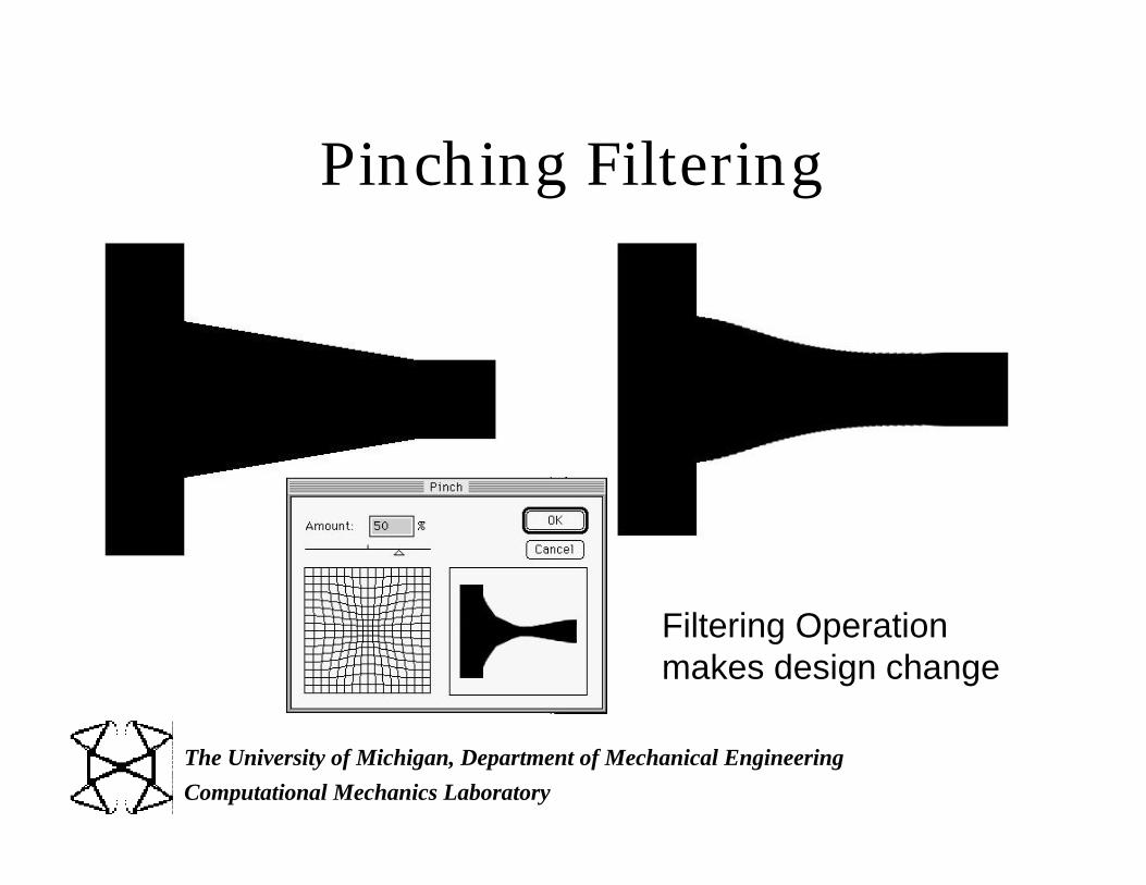
Pinching Filtering

Filtering Operationmakes design change



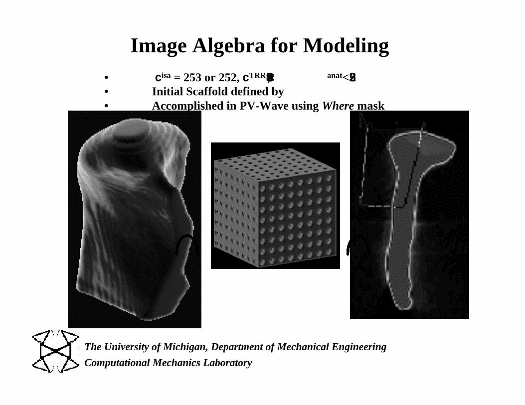
Image Algebra for Modeling• χisa = 253 or 252, χTRR = 255, 0 < χanat< 252• Initial Scaffold defined by • Accomplished in PV-Wave using Where mask



Resulted Finite Element Model

Scaffold/Bone Image Scaffold/Bone Mesh

Done by Dr. Scott Hollister using Voxelcon2.0



Image Based CAEl Voxelcon : a Derivative of OPTISHAPE

– CAD/CT/MRI Image Scan or Equivalent Ways– Image Based Automated CAE

l Mesh Generation

l Construction of Common Model for Multiple Analyses

l Load/Support Condition

l FE Analysis

– Image Based Design & Optimizationl OPTISHAPE for topology.layout design

– Rapid Prototype by Layered Manufacturing– Simulation of Material Processing (Casting etc)



Database : Image

l Rather than STLfiles,SLC files areconsidered

l SLC files are stored asIMAGES

l images are thencompressed

l 25K/slice x 500=7.5M



Image Regenerated



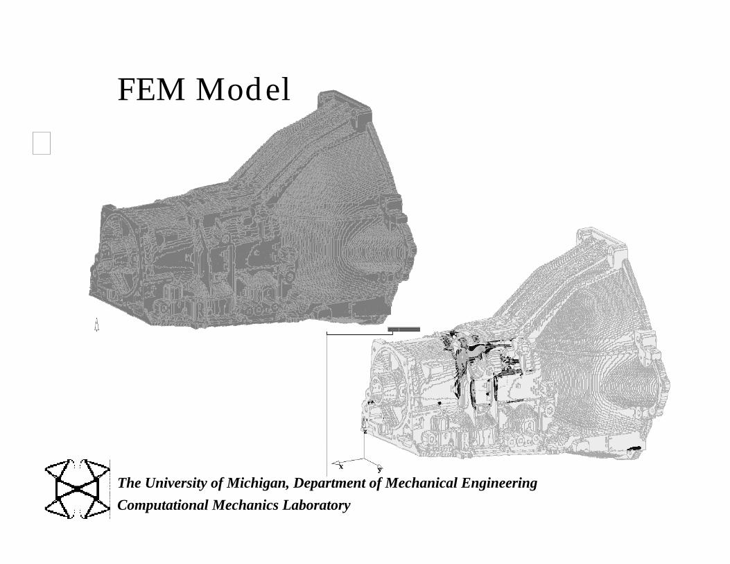
FEM Model



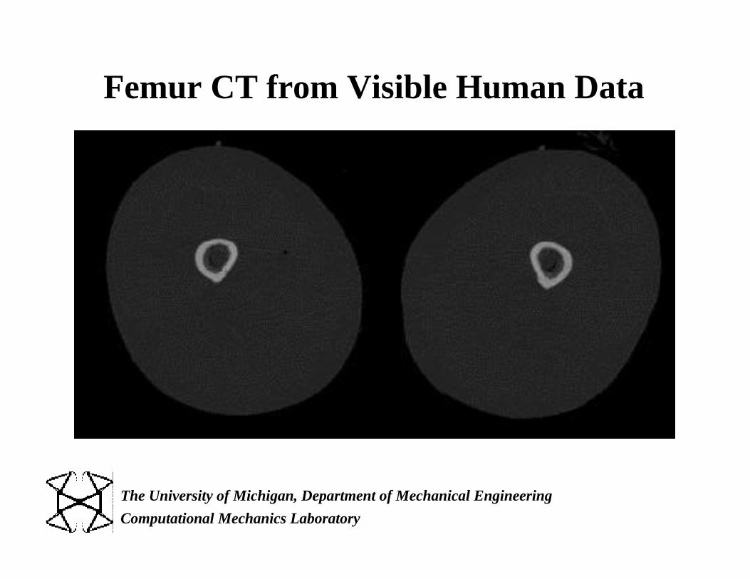
Femur CT from Visible Human Data



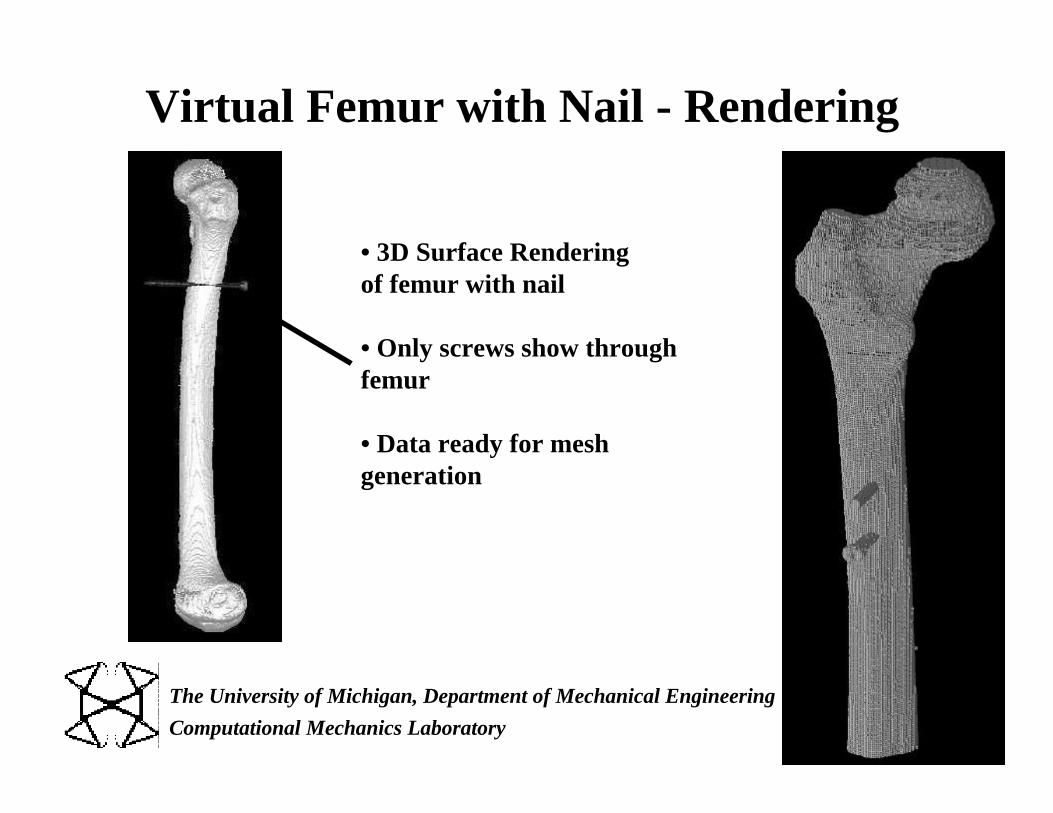
Virtual Femur with Nail - Rendering

• 3D Surface Renderingof femur with nail

• Only screws show throughfemur

• Data ready for meshgeneration



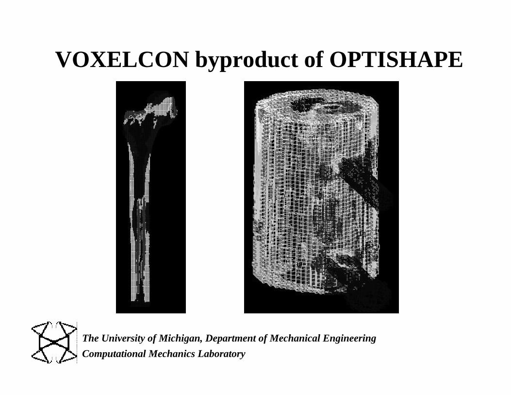
VOXELCON byproduct of OPTISHAPE



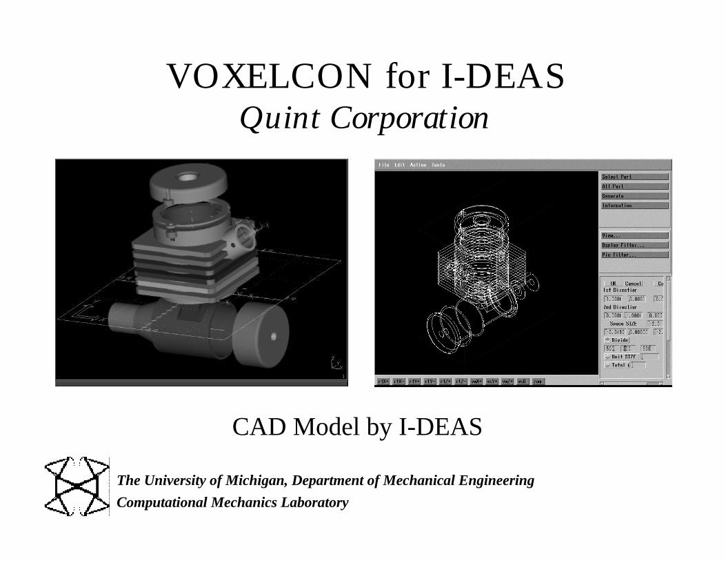
VOXELCON for I-DEASQuint Corporation

CAD Model by I-DEAS



VOXELCON for I-DEAS (2)

75M Voxel Elements 9.4 M Voxel Elements



OPTISHAPEQuint Corporation

Topology (NK, A. Diaz)Compliant Mechanisms (NK, S. Nishiwaki)

Shape (H. Azekami)Size (H. Miura)



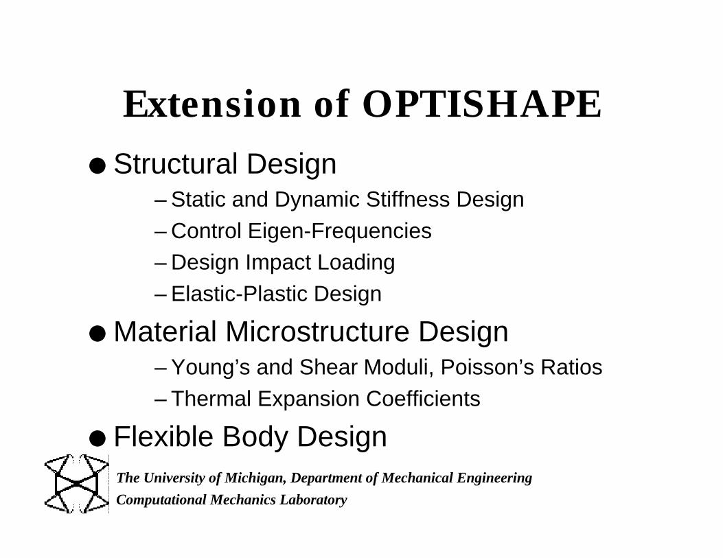
Extension of OPTISHAPEl Structural Design

– Static and Dynamic Stiffness Design– Control Eigen-Frequencies– Design Impact Loading– Elastic-Plastic Design

l Material Microstructure Design– Young’s and Shear Moduli, Poisson’s Ratios– Thermal Expansion Coefficients

l Flexible Body Design



New Extension ofOPTISHAPE

Piezocompositeand

Piezoelectric Actuator DesignFor Creation of New Value



Force

Displacement

Electric potential

Electric charge

Introduction

Mechanical Energy

Electrical Energy

Piezoelectric Material

Examples: Quartz (natural) Ceramic (PZT5A, PMN, etc…) Polymer (PVDF)



Applications

Pressure sensorsaccelerometersactuators,acoustic wave generation

ultrasonic transducers, sonar, hydrophonesetc...



cEijkl - stiffness property

eikl - piezoelectric strain propertyεS

ik - dielectric property

Tij - stress

Skl - strain

Ek - electric field

Di - electric displacement

Constitutive Equations of PiezoelectricMedium

T c S e E

D E e Sij ijkl

Ekl kij k

i ikS

k ikl kl

= −= +

ε

Elasticity equation

Electrostatic equation



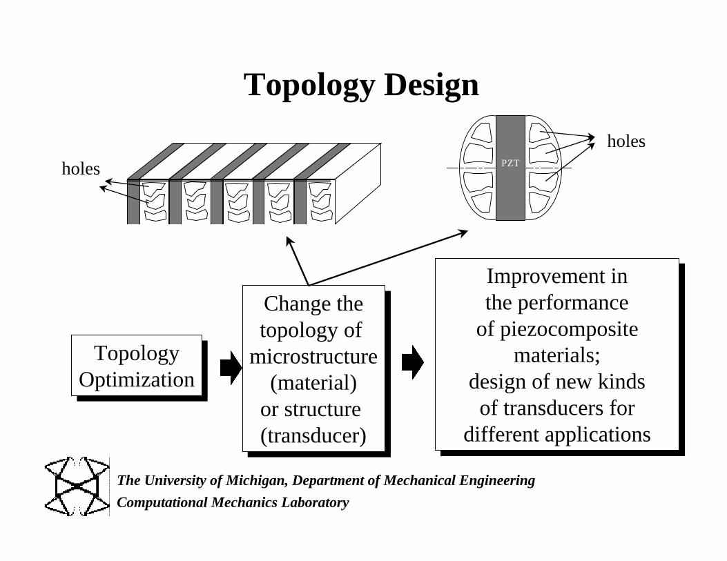
TopologyOptimization

Change thetopology of

microstructure(material)

or structure (transducer)

Improvement inthe performance

of piezocompositematerials;

design of new kindsof transducers for

different applications

PZT

holes

holes

Topology Design



x2

x1

Ω

t

Structure Design Domain

1

1y2

y1

θa

b

Material Design

Many Approaches : MDM

E x Eijklp

ijkl= 0

property

fraction of material in each point

Simple: Density Method

General:Homogenization Method

A point with no material

A point with material

microstructure

Structure Design



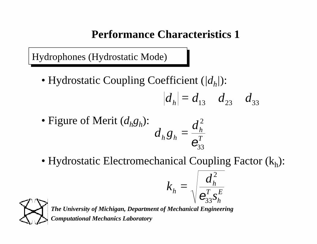
• Hydrostatic Coupling Coefficient (|dh|):

• Figure of Merit (dhgh):

• Hydrostatic Electromechanical Coupling Factor (kh):

Performance Characteristics 1

kd

shh

ThE=

2

33ε

d gd

h hhT=2

33ε

Hydrophones (Hydrostatic Mode)

d d d dh = + +13 23 33



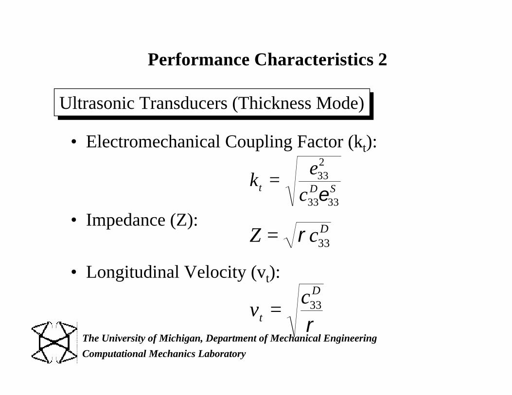
• Electromechanical Coupling Factor (kt):

• Impedance (Z):

• Longitudinal Velocity (vt):

Performance Characteristics 2

ke

ct D S= 332

33 33ε

Z cD= ρ 33

vc

t

D

= 33

ρ

Ultrasonic Transducers (Thickness Mode)

47Computational Mechanics Laboratory


(Poled in the 3 direction)

Reference unit cell for comparison: 2-2 piezocomposite

PZT5APolymer (Spurr)

0102030405060708090

100

0 0.2 0.4 0.6 0.8 1

Ceramic Volume Fraction

d h (

pC/N

)

0

500

1000

1500

2000

2500

3000

3500

0 0.2 0.4 0.6 0.8 1


d hg h

(fP

a-1)

0

0.02

0.04

0.06

0.08

0.1

0.12

0.14

0.16

0 0.2 0.4 0.6 0.8 1


k h

0

0.1

0.2

0.3

0.4

0.5

0 0.2 0.4 0.6 0.8 1


k t

dh

dhgh

kh kt



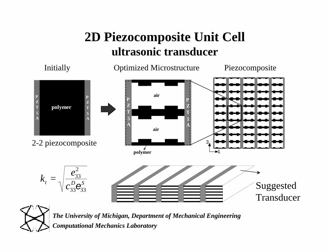
air

air

polymer

PZT5A

PZT5A

1

3

2D Piezocomposite Unit Cellultrasonic transducer

ke

ct D S= 332

33 33ε

polymer

PZT5A

PZT5A

Initially Optimized Microstructure Piezocomposite

2-2 piezocomposite

Suggested Transducer



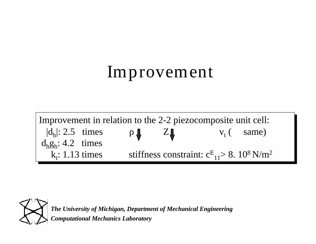
Improvement

Improvement in relation to the 2-2 piezocomposite unit cell: |dh|: 2.5 times ρ Z vt ( same) dhgh: 4.2 times kt: 1.13 times stiffness constraint: cE

11> 8. 108 N/m2

⇒ ≅



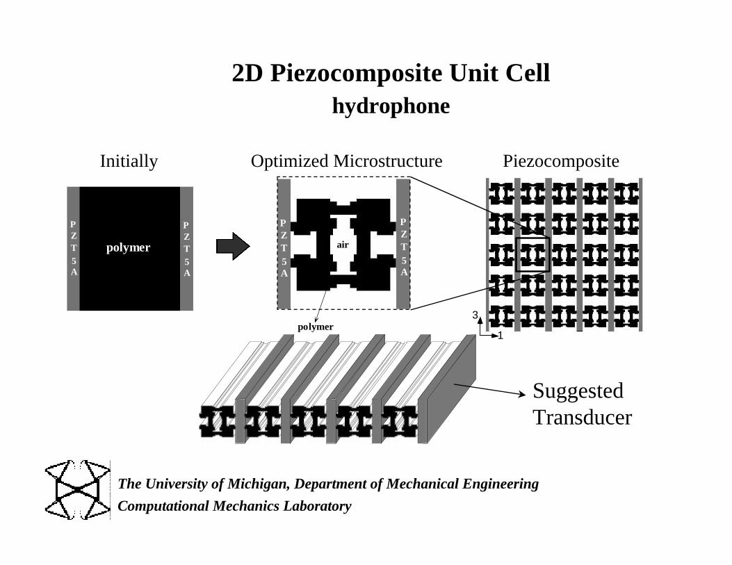
air

PZT5A

PZT5A

polymer

2D Piezocomposite Unit Cellhydrophone

Suggested Transducer

polymer

PZT5A

PZT5A

1

3




Improvement

Improvement in relation to the 2-2 piezocomposite unit cell: |dh|: 2.8 times ρ Z vt ( same)dhgh: 7.1 times kt: 1.13 times stiffness constraint: cE

11>8.108N/m2

⇒ ≅



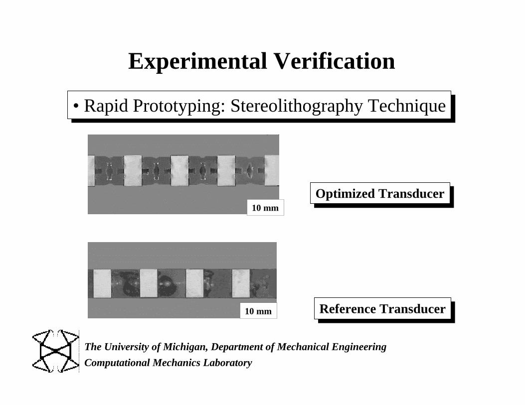
Experimental Verification

• Rapid Prototyping: Stereolithography Technique

Optimized Transducer

Reference Transducer

10 mm

10 mm



Experimental Result

bar ofPZT5Apolymer part

Measured Performances dh(pC/N) dhgh (fPa-1) kt

Reference 9.1 13.2 0.69Optimized 246. 10400. 0.70(Simulation) (229.) (10556.) (0.66)



PZT5A

air


PZT5A

1

3


“optimized porous ceramic”



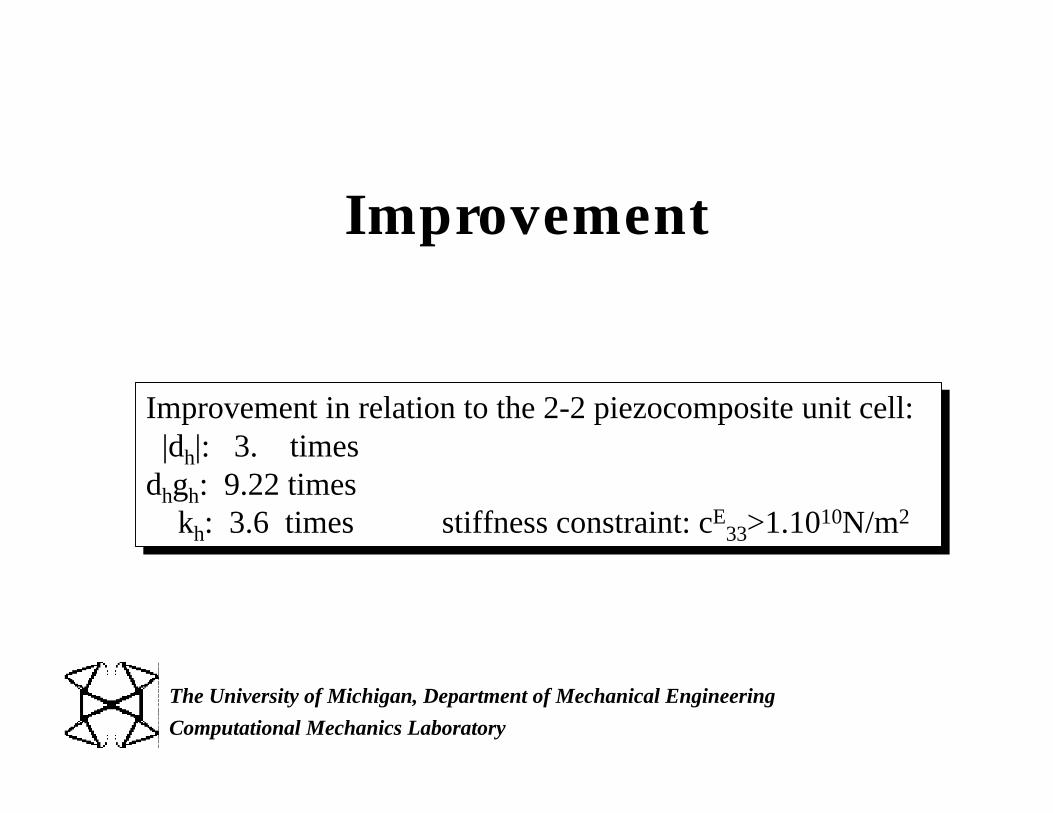
Improvement

Improvement in relation to the 2-2 piezocomposite unit cell: |dh|: 3. timesdhgh: 9.22 times kh: 3.6 times stiffness constraint: cE

33>1.1010N/m2



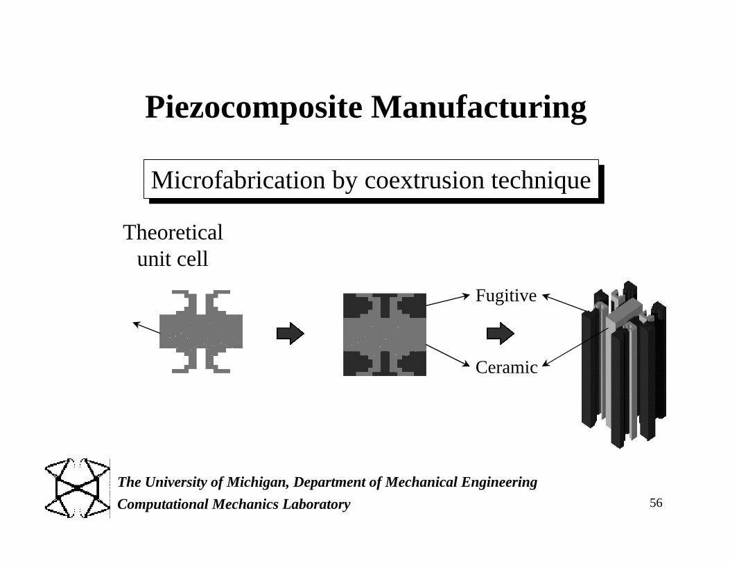
Piezocomposite Manufacturing

Theoretical unit cell

Fugitive

Ceramic

Microfabrication by coextrusion technique



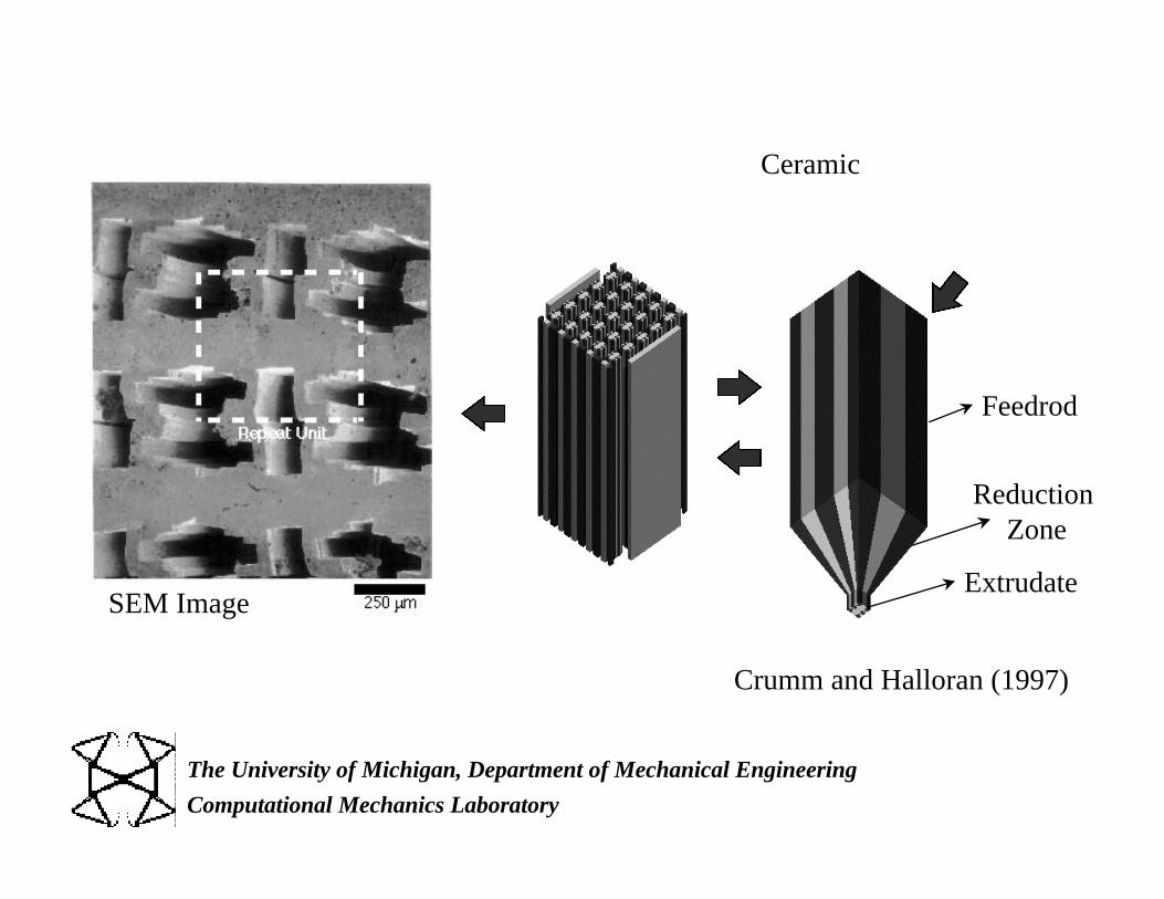
Ceramic

Feedrod

Reduction Zone

ExtrudateSEM Image

Crumm and Halloran (1997)



1

380 µm

Measured Performances dh(pC/N) dhgh (fPa-1) Solid PZT 68. 220.

Optimized 308. 18400. (Simulation) (257.) (19000.)

Theoretical Prototype



zy

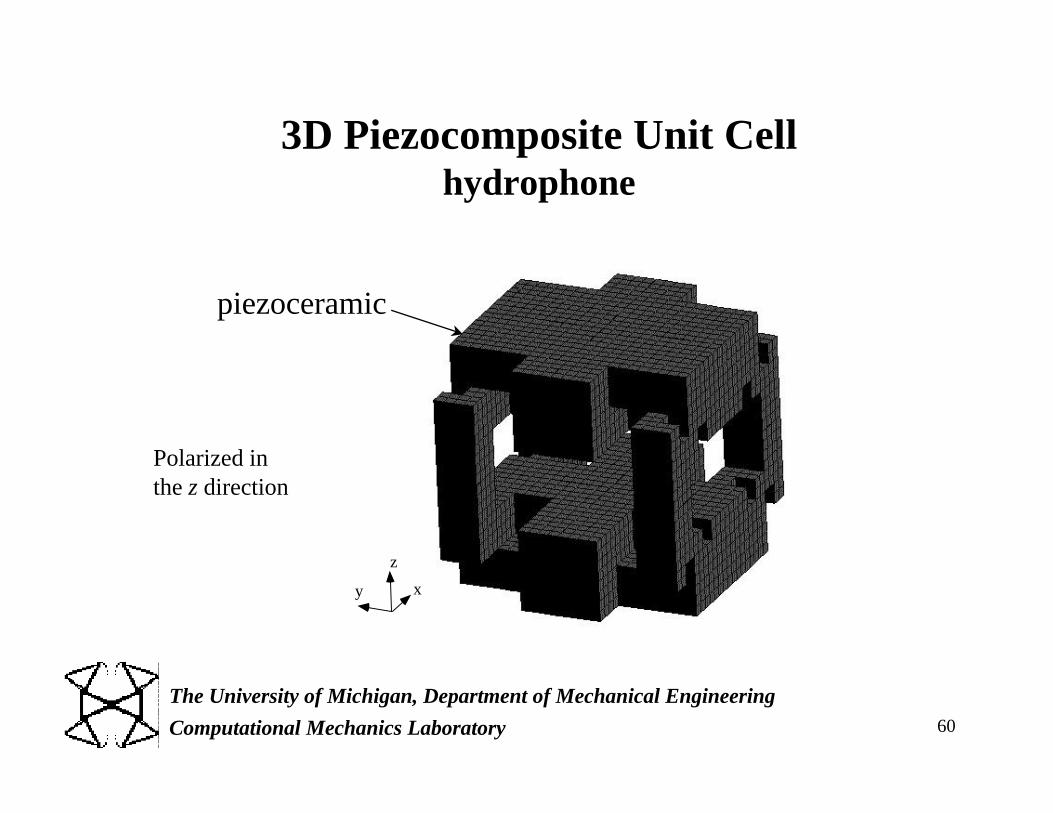
x

piezoceramic


Poled in the z direction



xy

z

piezoceramic

Polarized in the z direction




OPTISHAPE

Compliant Mechanism Design

A New Release



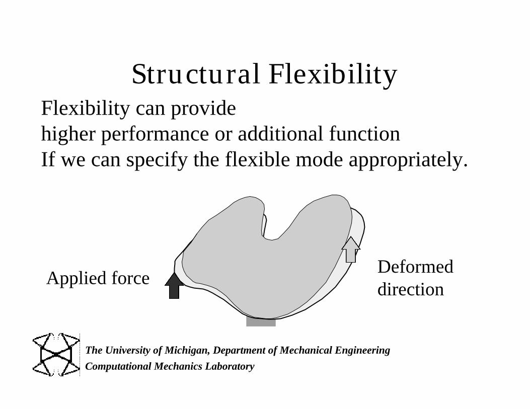
Structural FlexibilityFlexibility can providehigher performance or additional functionIf we can specify the flexible mode appropriately.

Applied forceDeformeddirection



Kinematic Synthesis

Based on traditional rigid body kinematics

Lumped compliance (Pivot) Stress concentration

Her and Midha (1986), Howell and Midha (1994), (1996)

Lumped compliant mechanism



Based on the topology optimization method

Distributed compliant mechanism

Continuum Synthesis

Ananthasuresh et al. (1994, 1995), Frecker et al. (1997)Sigmund (1995), (1996), Larsen et al. (1996)



Flexibility and Stiffnesst

1 u1 u

1

t2

Γt 2

Γt 1

Maximize L2u

1( )= t2 • u

1dΓΓt 2∫ Mutual Mean Compliance (MMC)

Mean Compliance (MC)Minimize L1

u1( )= t

1 • u1dΓ

Γt1∫

Flexibility at Γt

2

Stiffness at Γt1

Applied traction

Dummy traction



Formulation of MutualStiffness

Minimize L2u

1( ) = t2 • u

1 dΓΓ t 2∫

Stiffness at Γt

2 with respect to t1

Applied traction

Γt1

Γt 2

Deformed shape

Dummy traction

Slide along the line

t1

t2



Compliant Mechanism Design

Kinematic function

Structural function

Flexibility

Stiffness

Reaction force

+ +

Applied force Mutualstiffness

ConstrainedMotion

Maximize (MMC)

Minimize ( MC)∑



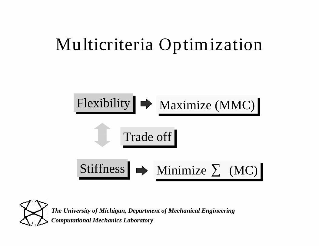
Multicriteria Optimization

Flexibility

Stiffness

Maximize (MMC)

Minimize (MC)∑

Trade off



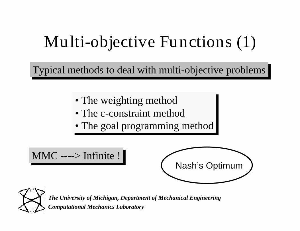
Multi-objective Functions (1)

Typical methods to deal with multi-objective problems

• The weighting method• The ε-constraint method• The goal programming method

MMC ----> Infinite !Nash’s Optimum



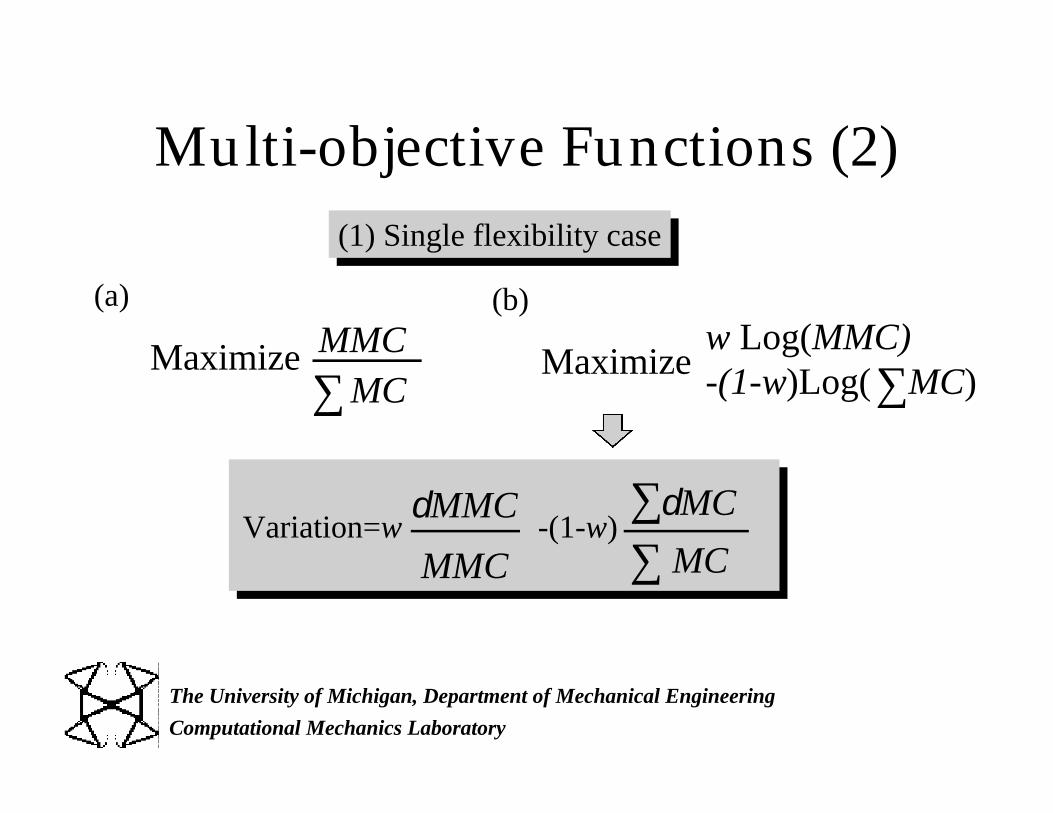
Multi-objective Functions (2)

Maximize MMCMC

(a)

∑w Log(MMC)-(1-w)Log( MC)∑

(1) Single flexibility case

(b)

Maximize

Variation=w -(1-w)MMC MC∑δMMC δMC∑



Multi-objective functions (3)(2) Displacement single flexibility case

MMC Constraint

(3) Multi-flexibility case

Maximize-1/Cf Log( Exp(-Cf MMC))∑ i

1/Cs Log( Exp(Cs MC))j∑

Minimize MC∑



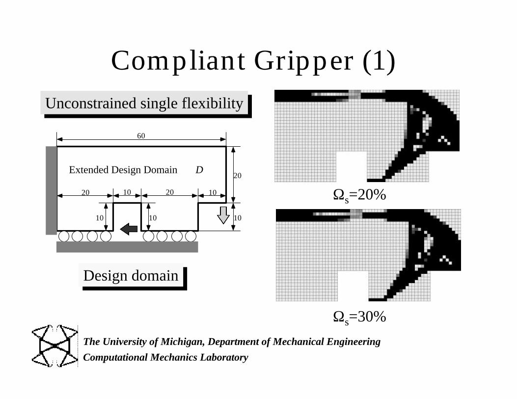
Compliant Gripper (1)Unconstrained single flexibility

60

20 20

20

10

10

10

10

10

Extended Design Domain D

Design domain

Ωs=20%

Ωs=30%



Compliant Gripper (2)

Deformed shape

Mises stress

Extracted image design



Torsional CompliantMechanism

Extracted image design

ExtendedDesignDomain D

2010

10

10

10

Design domain

: Applied force: Direction of deformation

Unconstrained single flexibility



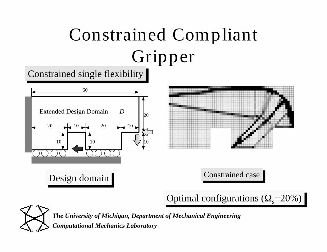
Constrained CompliantGripper

Constrained single flexibility

60

20 20

20

10

10

10

10

10

Extended Design Domain D

Design domain

Optimal configurations (Ωs=20%)

Constrained case



Unified Design of Structures andMechanisms

Unified design approachCurrent design approach

LargeFriction force

Sub frame

Unified parts

SmallFriction force

Small change ofchamber angle

Strut-type suspension

Large change ofchamber angle



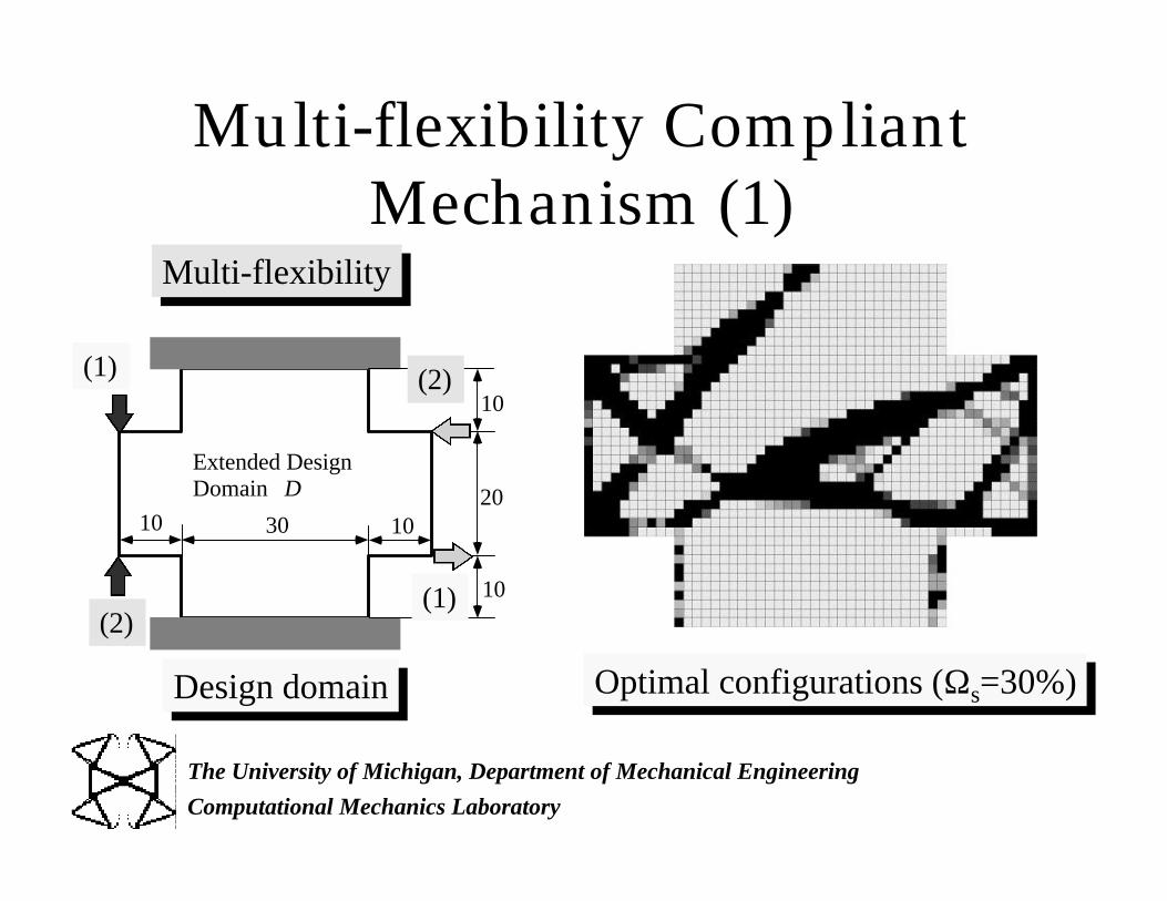
Multi-flexibility CompliantMechanism (1)

20

10

10

10 1030

Extended DesignDomain D

Multi-flexibility

Design domain

(1)

(1)(2)

(2)

Optimal configurations (Ωs=30%)



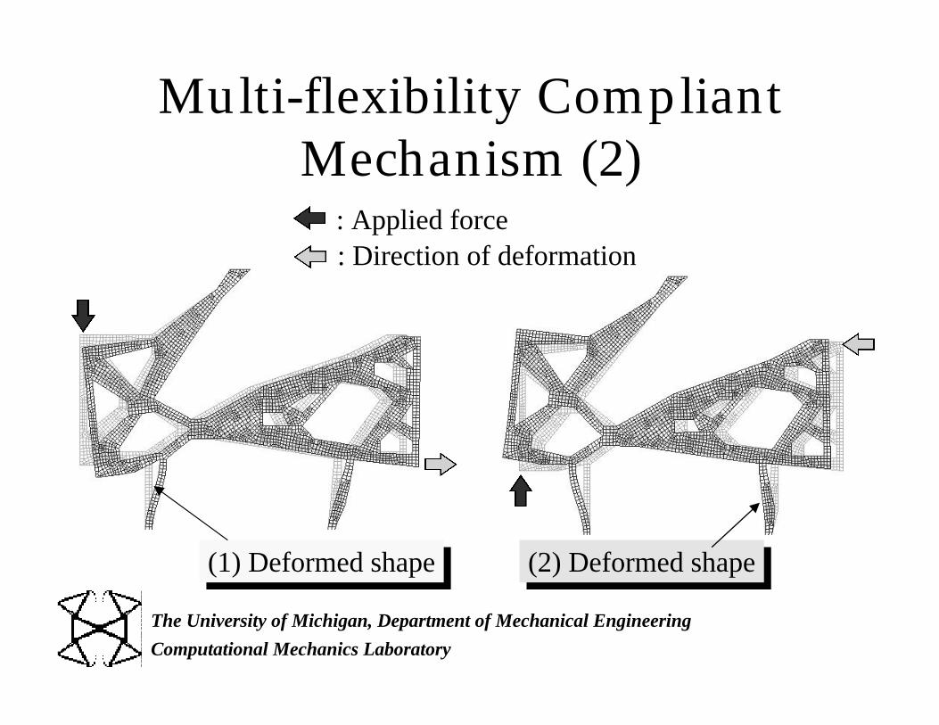
Multi-flexibility CompliantMechanism (2)

(1) Deformed shape (2) Deformed shape

: Applied force: Direction of deformation



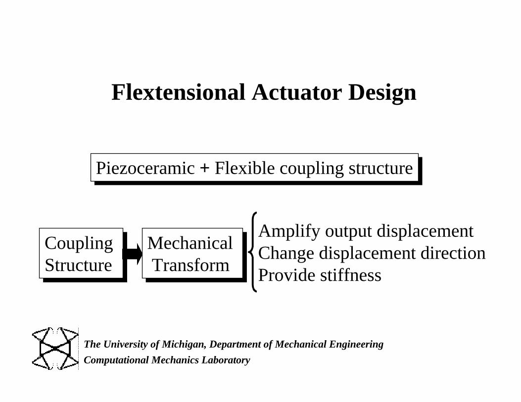
Flextensional Actuator Design

Piezoceramic + Flexible coupling structure

Amplify output displacement Change displacement direction Provide stiffness

Coupling Structure

Mechanical Transform



OPTISHAPE

Actuator Design

A New Capabilityto be Implemented



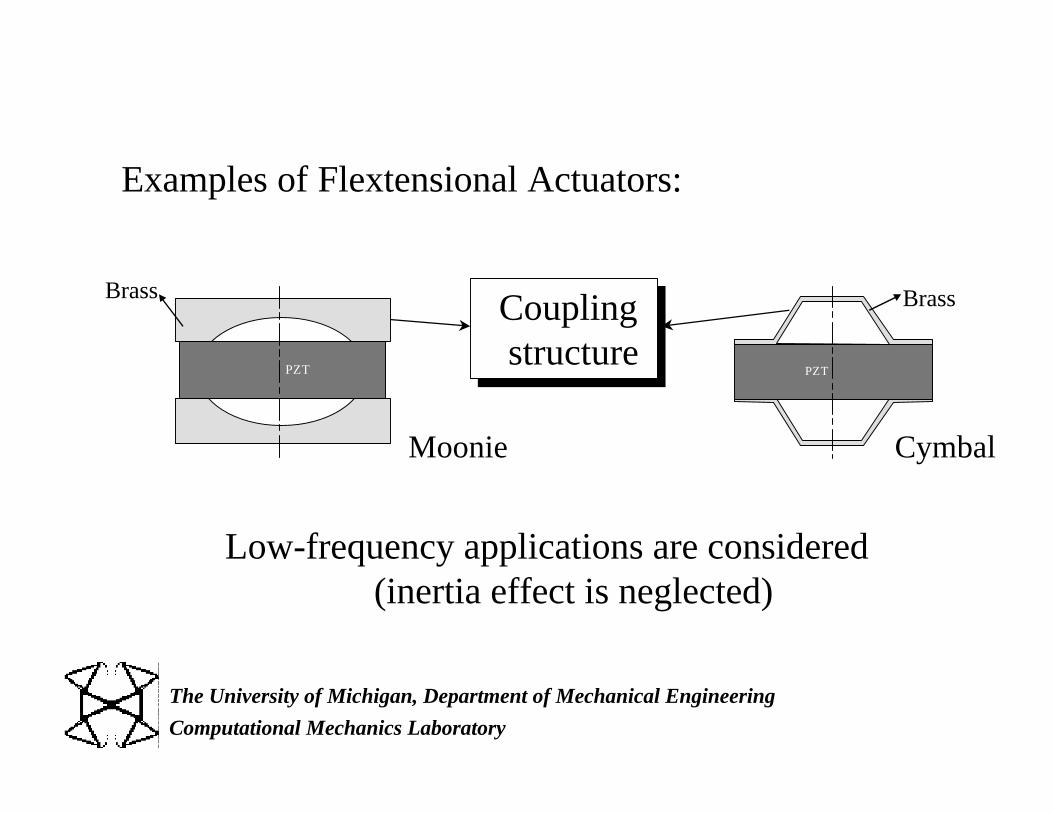
Examples of Flextensional Actuators:

Moonie Cymbal

Coupling structure

PZT PZT

Low-frequency applications are considered (inertia effect is neglected)

Brass Brass



PZT

x1

x3

Q1

F2 1

Maximize outputdisplacement (∆u)

Max (mean transduction)

Maximize blockingforce

Min (mean compliance)

( trade-off )

u3

∆u-F2

PZT

φ2

body

φ2 1

t Q

U3

U F3 2

t −



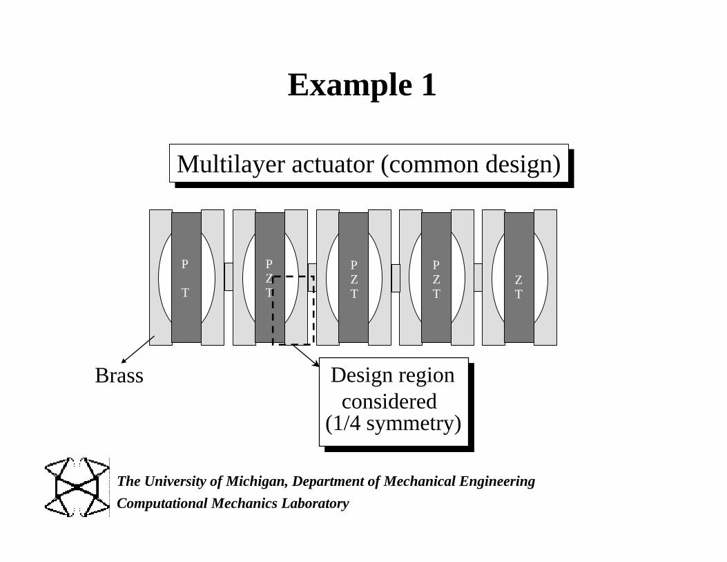
Example 1

Multilayer actuator (common design)

P

T

PZT

PZT

PZT

ZT

Design region considered(1/4 symmetry)

Brass



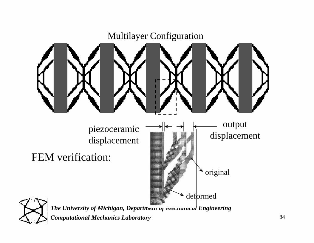
Multilayer Configuration

FEM verification:

outputdisplacement

piezoceramicdisplacement

original

deformed



Example 2

FEM verification:

deformed

original

Optimal topology

Piezoceramicoutputdispl.

(1/4 symmetry)

∆u

w=0.5

Design Domain (Brass)

1

3PZT

B

Design Domain (Brass)

Q



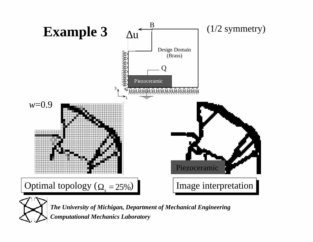
Example 3Design Domain (Brass)

Piezoceramic

Q

B

1

3

(1/2 symmetry)∆u

Optimal topology ( )Ωs = 25%

Piezoceramic

w=0.9

Image interpretation



Structural Optimization in MagneticFields

Future OPTISHAPE Capability



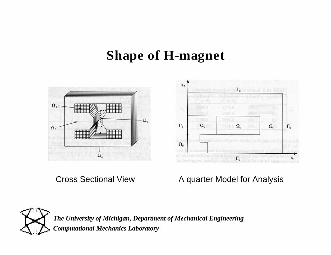
Shape of H-magnet

Cross Sectional View A quarter Model for Analysis



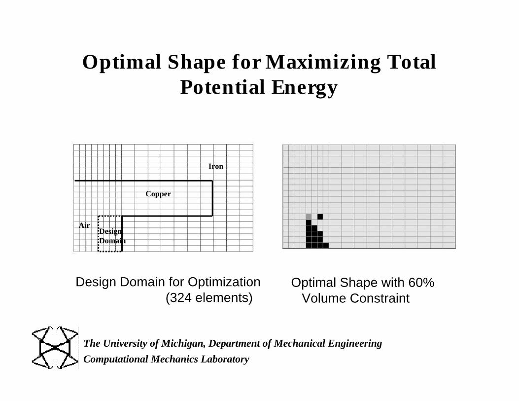
Optimal Shape for Maximizing TotalPotential Energy

Iron

Copper

AirDesignDomain

Design Domain for Optimization (324 elements)

Optimal Shape with 60% Volume Constraint



Analysis of the Optimal Shape

Vector Potential Flux Density

Increase the value of Flux Densities in Design Domain (25 - 40%)Stabilize the Flux Densities



Optimal Shape for Prescribed Uniform Fields (432 element model)

Prescribed Bx = -0.18 Prescribed Bx = -0.18, By = 0.05

Prescribed Bx = -0.18 Prescribed Bx = -0.18 By = 0.05

Ave. of x components -0.18298E+00 -0.16645E+00

Ave. of y components 0.69363E-01 0.38788E-01

Stand. Dev. of x components 0.62515E-01 0.57342E-01

Stand. Dev. of y components 0.68198E-01 0.46641E-01



Optimal Shape of the Design Domainfor Prescribed Uniform Fields

(3-layer, 432 element model)

Prescribed Bx = -0.20 Prescribed Bx = -0.20, By = 0.05

Prescribed Bx = -0.18 Prescribed Bx = -0.18 By = 0.05

Ave. of x components -0.20712E+00 -0.20706E+00

Ave. of y components - 0.44251E-01

Stand. Dev. of x components 0.87911E-01 0.69931E-01

Stand. Dev. of y components - 0.57347E-01



Research Issue in OPTISHAPE

Material Design OptimizationYoung’s & Shear Moduli

Poisson’s RatiosThermal Exapansion Coefficients

Electro-magnetic Properties



Following ToDr. O. Sigmund

Technical University of Denmark

Jun Ono Fonsecaand

Bing-Chung Chen



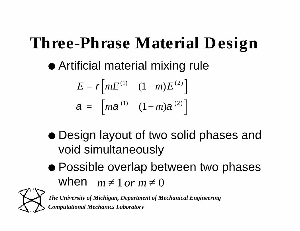
Three-Phrase Material Designl Artificial material mixing rule

l Design layout of two solid phases andvoid simultaneously

l Possible overlap between two phaseswhen

E mE m E

m m

= + −

= + −

ρ

α α α

( ) ( )

( ) ( )

( )

( )

1 2

1 2

1

1

m or m≠ ≠1 0



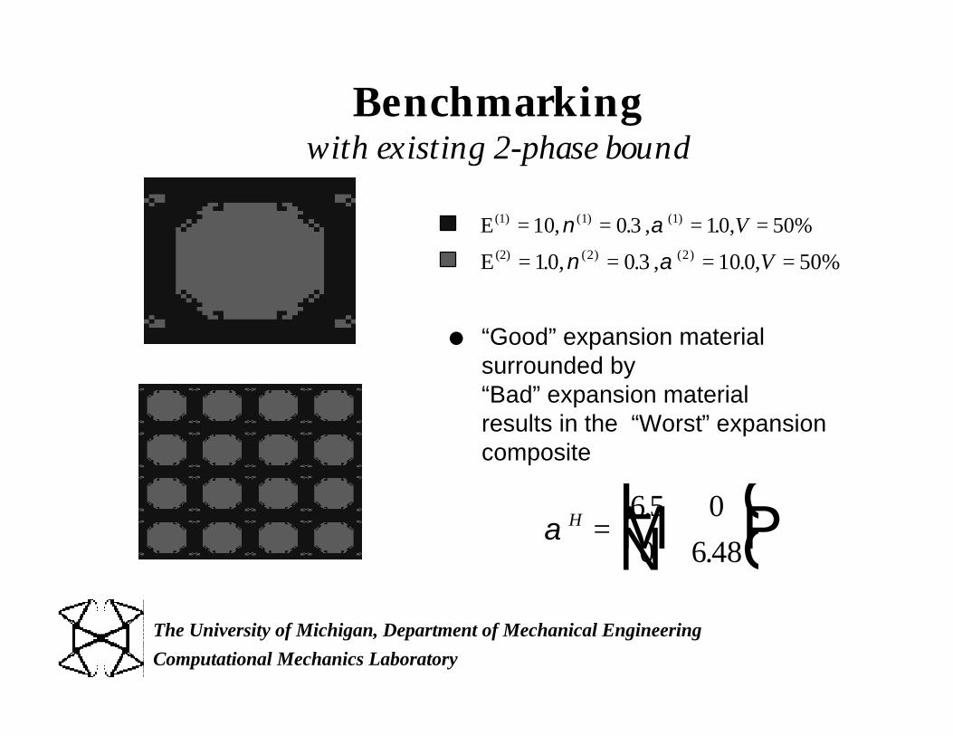
Benchmarkingwith existing 2-phase bound

E(1) = = = =10 0 3 10 50%1 1, . , . ,( ) ( )ν α V

E (2) = = = =10 0 3 10 0 50%2 2. , . , . ,( ) ( )ν α V

α H =LNM

OQP

6 5 0

0 6 48

.

.

l “Good” expansion materialsurrounded by“Bad” expansion materialresults in the “Worst” expansioncomposite



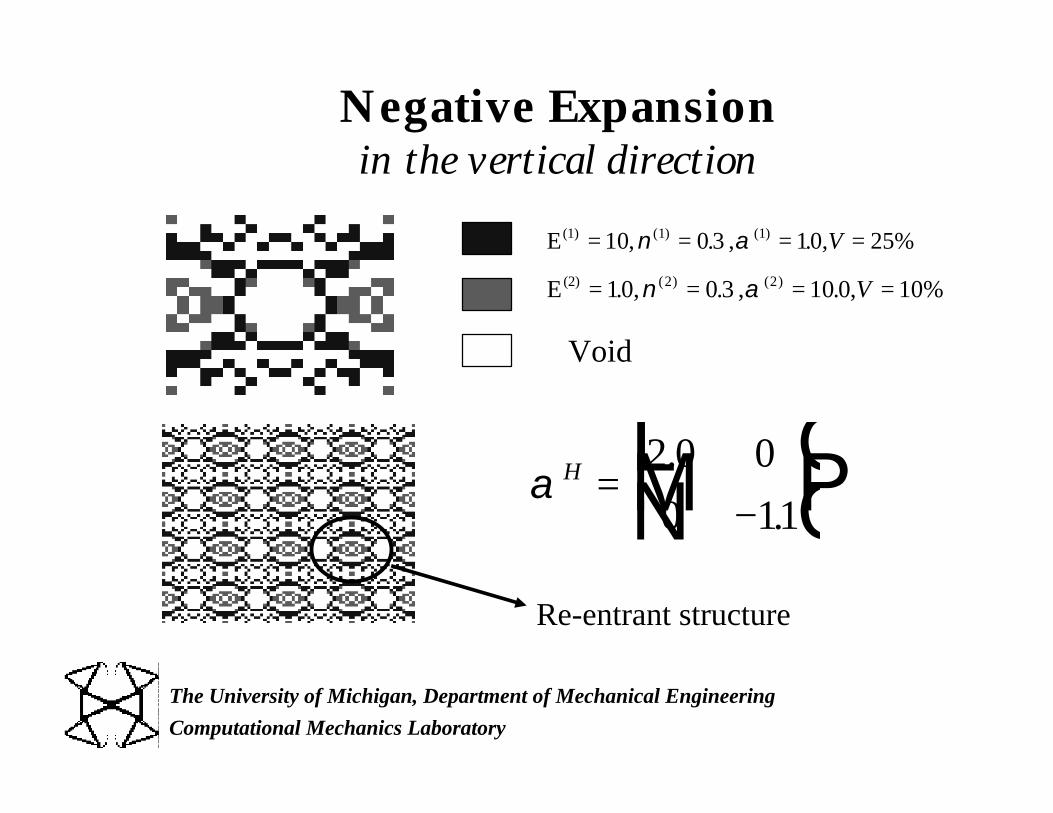
Negative Expansionin the vertical direction

E(1) = = = =10 0 3 10 25%1 1, . , . ,( ) ( )ν α V

E (2) = = = =10 0 3 10 0 10%2 2. , . , . ,( ) ( )ν α V

Void

α H =−

LNM

OQP

2 0 0

0 11

.

.

Re-entrant structure



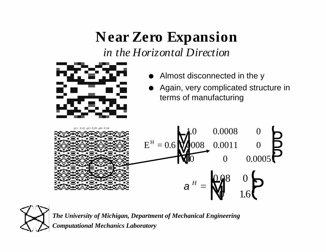
p1= 0.41 p2= 0.05 p0= 0.54

Near Zero Expansionin the Horizontal Direction

α H =LNM

OQP

0 08 0

0 16

.

.

EH =L

NMMM

O

QPPP

0 6

1 0 0 0008 0

0 0008 0 0011 0

0 0 0 0005

.

. .

. .

.

l Almost disconnected in the y

l Again, very complicated structure interms of manufacturing



Construction of three-phase material bytwo stage design

l Given distribution of phase 1, design phase 2distribution, excluding the domain occupied byphase 1

l Mark phase 2 as exclusion, design phase 1l The final micro-structure should be non-

complex and easy to manufacture.

Design phase 2Mark phase 1as excluded

Design phase 2Mark phase 1as excluded



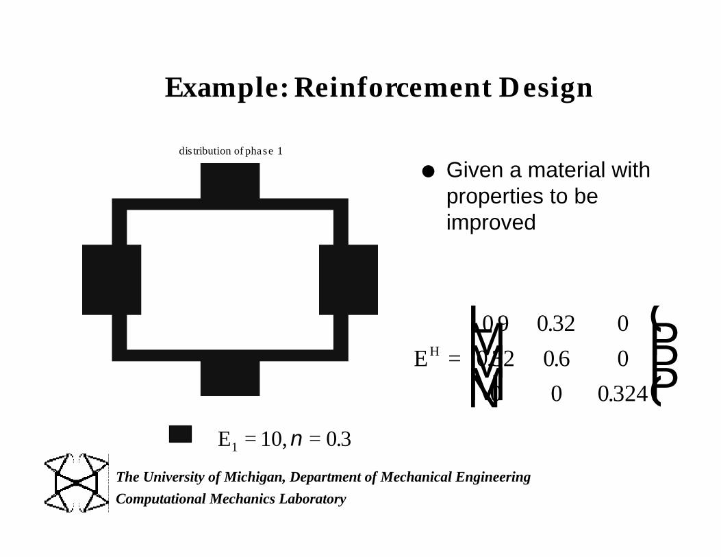
Example: Reinforcement Design

dis tribution of phase 1

l Given a material withproperties to beimproved

EH =L

NMMM

O

QPPP

0 9 0 32 0

0 32 0 6 0

0 0 0 324

. .

. .

.

E1 = =10 0 3, .ν



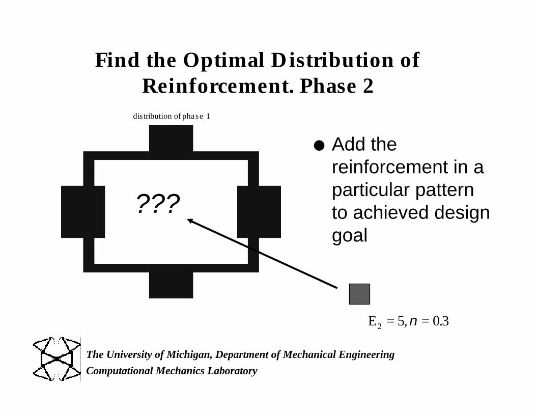
Find the Optimal Distribution ofReinforcement. Phase 2

E2 = =5 0 3, .ν

??


???

l Add thereinforcement in aparticular patternto achieved designgoal



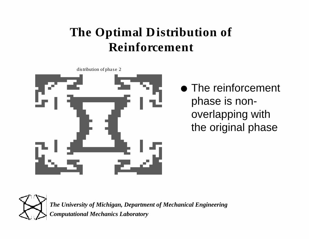
The Optimal Distribution ofReinforcement

l The reinforcementphase is non-overlapping withthe original phase




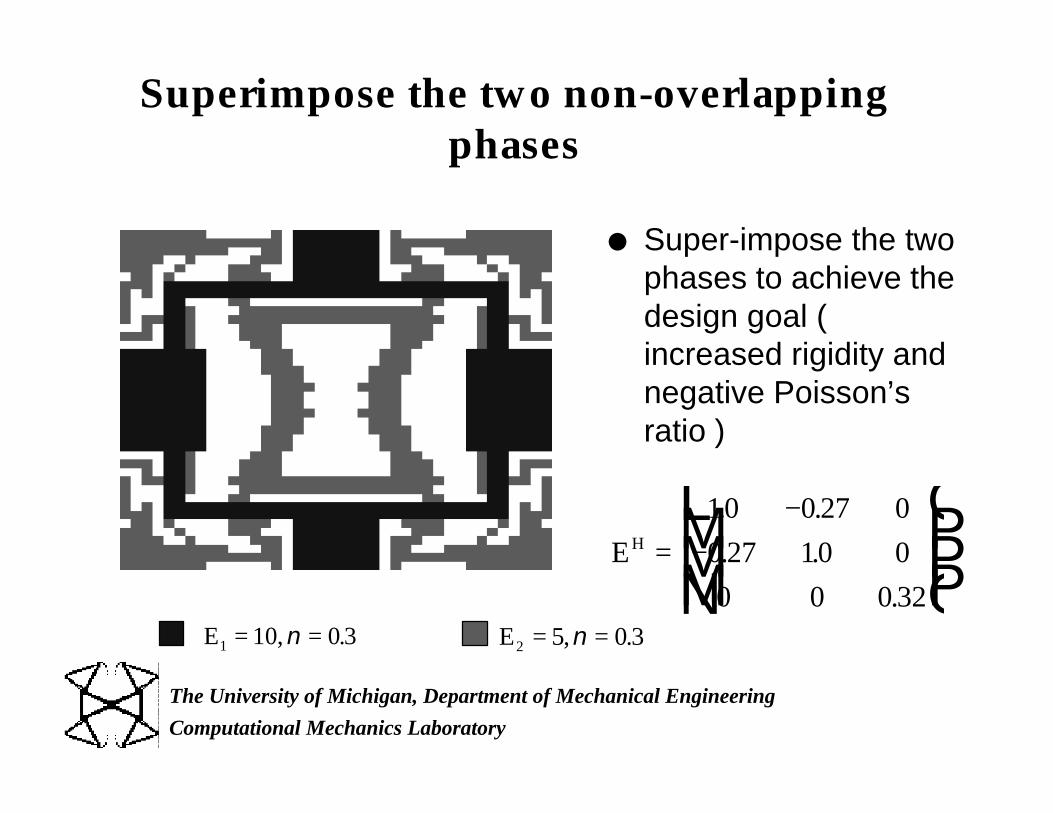
Superimpose the two non-overlappingphases

l Super-impose the twophases to achieve thedesign goal (increased rigidity andnegative Poisson’sratio )

E2 = =5 0 3, .ν

EH =−

−L

NMMM

O

QPPP

10 0 27 0

0 27 10 0

0 0 0 32

. .

. .

.E1 = =10 0 3, .ν



E(1) = = = =10 0 3 10 30%1 1, . , . ,( ) ( )ν α V

E (2) = = = =10 0 3 10 0 25%2 2, . , . ,( ) ( )ν α V

Void

distribution of phase 1

Negative expansion in the horizontaldirection

l Stretch in the y due to temperature rise

l Shrink in the x due to Poisson’s effect

l Unusual CTE material must encompassstructure-like mechanism



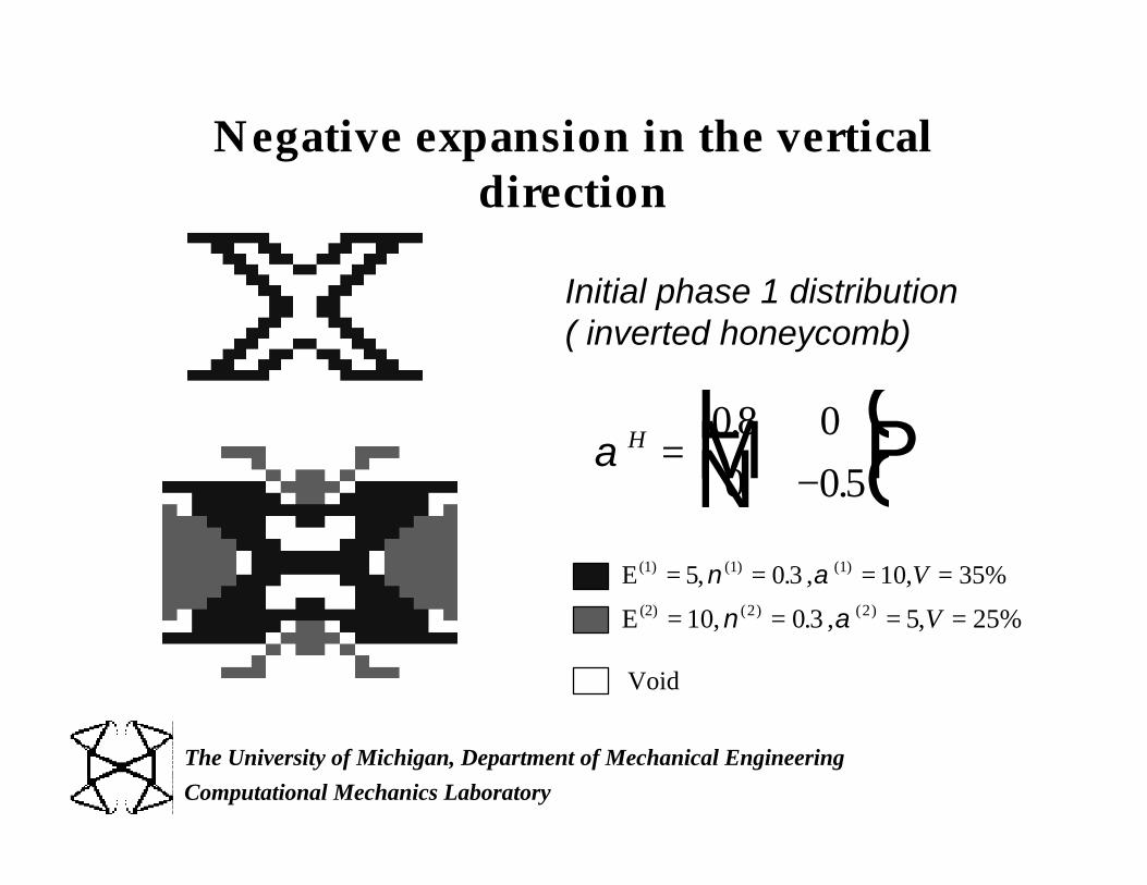
Negative expansion in the verticaldirection

E(1) = = = =5 0 3 10 35%1 1, . , ,( ) ( )ν α V

E (2) = = = =10 0 3 5 25%2 2, . , ,( ) ( )ν α V

Void

α H =−

LNM

OQP

08 0

0 0 5

.

.

Initial phase 1 distribution ( inverted honeycomb)



Near zero Thermal Expansion

Phase 1 Phase 2

α H =LNM

OQP

0 22 0

0 0 21

.

.

E (1) = = = =5 0 3 10 25%1 1, . , ,( ) ( )ν α V

E (2) = = = =10 0 3 5 30%2 2, . , ,( ) ( )ν α V



Topology Optimization AlgorithmExamination / Research

Various Filtering SchemesProposedusing SLP



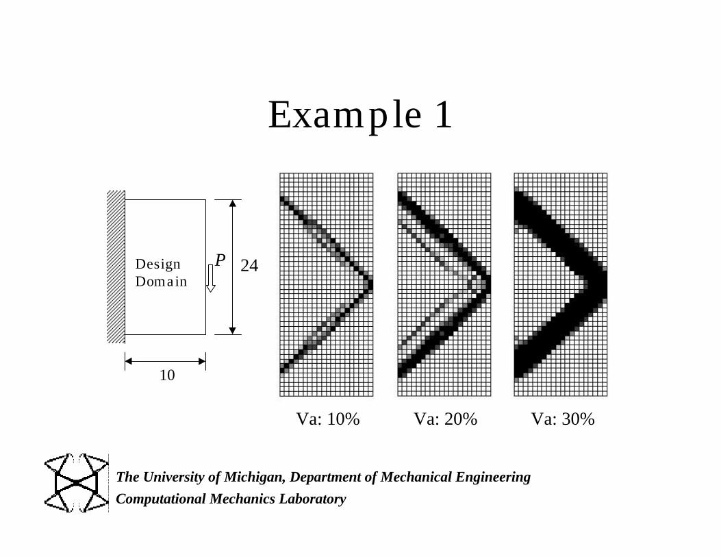
Example 1

24

10

PDesignDomain

Va: 10% Va: 20% Va: 30%



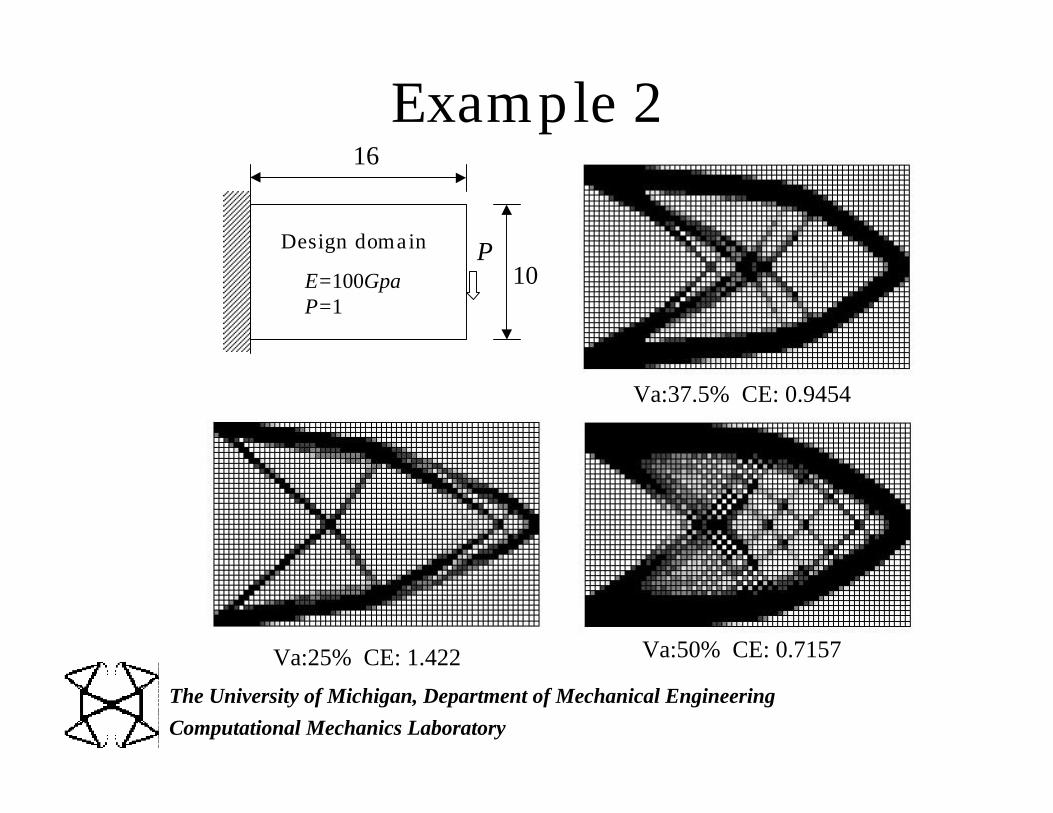
Example 2

10

16

Design domain PE=100GpaP=1

Va:37.5% CE: 0.9454

Va:50% CE: 0.7157Va:25% CE: 1.422



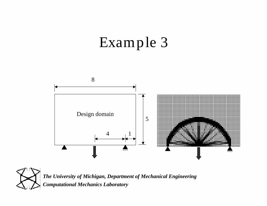
Example 3

Design domain

4 1

8

5



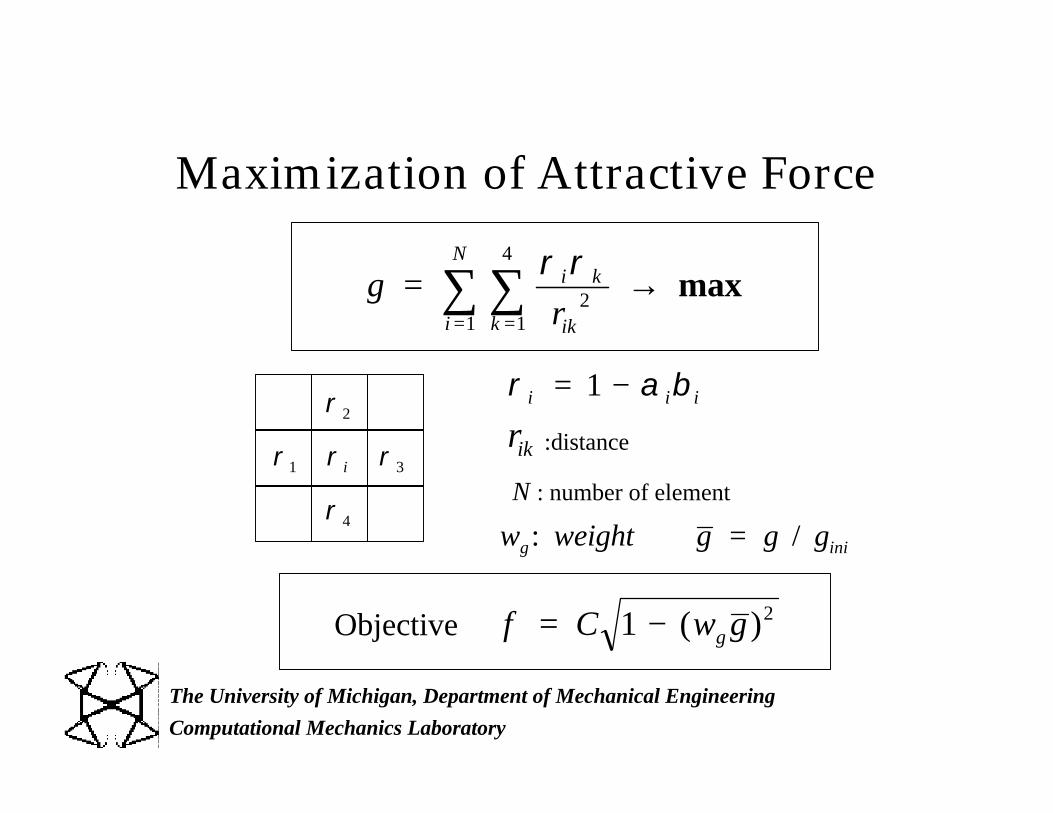
Maximization of Attractive Force

ρ i

ρ2

ρ1 ρ 3

ρ4

ρ α βi i i= −1

rik :distance

gri k

ikki

N

= →==

∑∑ ρ ρ2

1

4

1

max

w weight g g gg ini: /=N : number of element

f C w gg= −1 2( )Objective



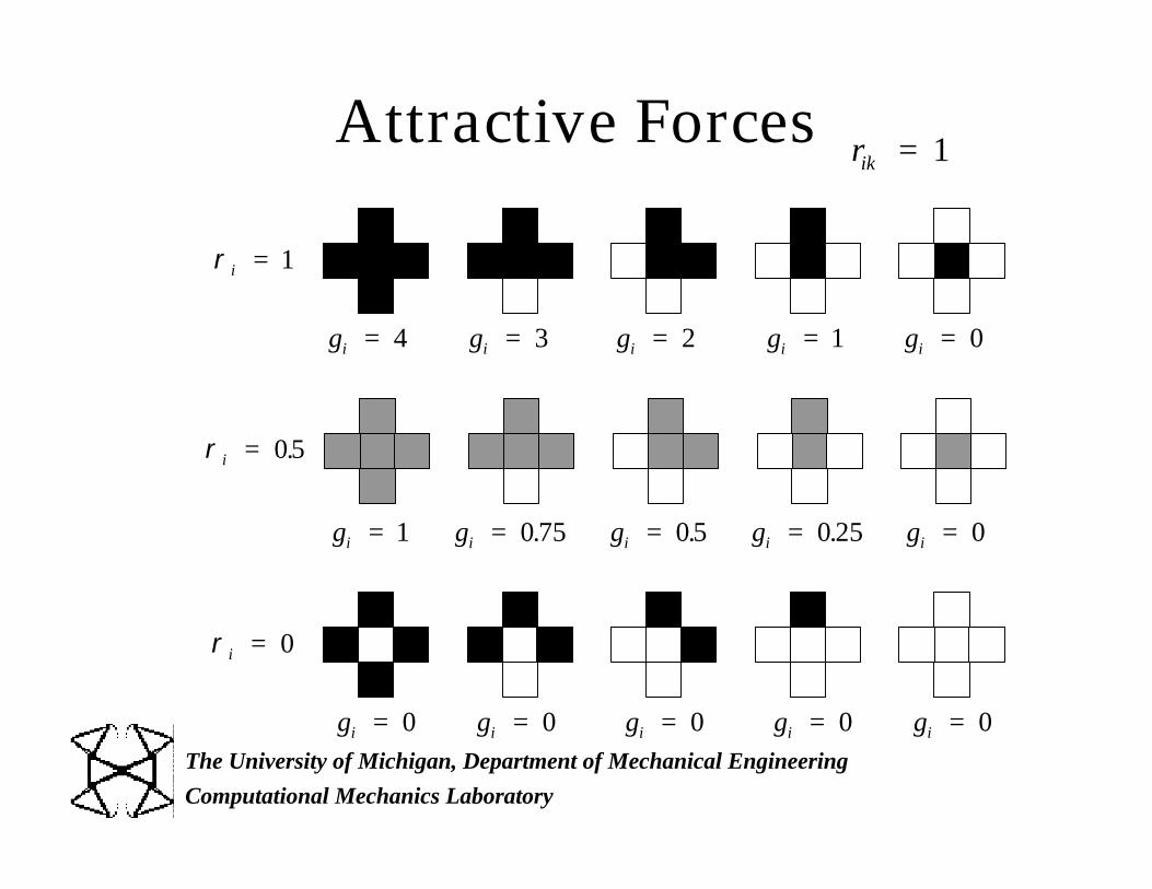
Attractive Forces

gi = 4 gi = 3 gi = 2 gi = 1 gi = 0

ρ i = 1

ρ i = 0 5.

gi = 1 gi = 0 75. gi = 0 5. gi = 0 25. gi = 0

ρ i = 0

gi = 0 gi = 0 gi = 0 gi = 0 gi = 0

rik = 1



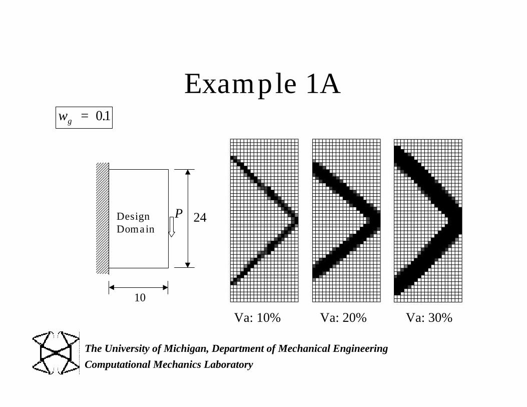
Example 1A

24

10

PDesignDomain

Va: 10% Va: 20% Va: 30%

wg = 01.



Example 2A

10

16


Va:37.5% CE: 0.9576

Va:50% CE: 0.7275Va:25% CE: 1.499

wg = 01.



Example 3A

Design domain

4 1

8

5

wg = 01.



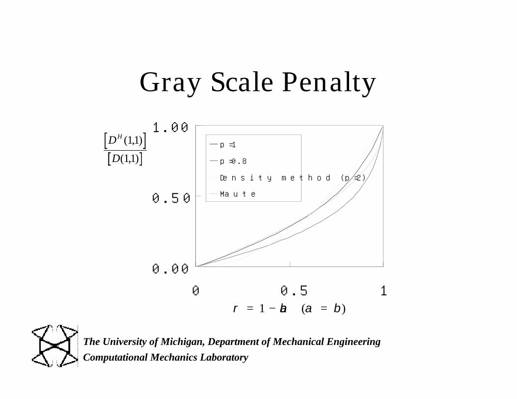
Gray Scale Penalty

0.00

0.50

1.00

0 0.5 1

p=1

p=0.8

Density method (p=2)

Maute

D

D

H ( , )

( , )

11

11

ρ αβ α β= − =1 ( )



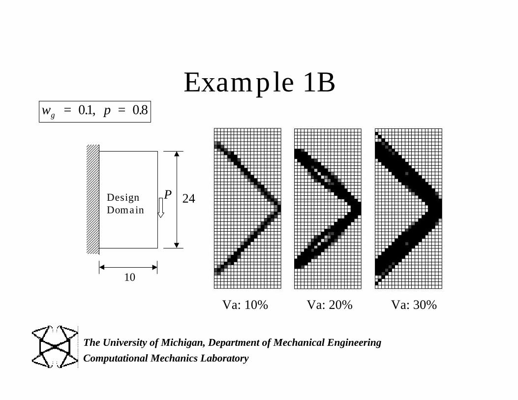
Example 1B

24

10

PDesignDomain

Va: 10% Va: 20% Va: 30%

w pg = =01 0 8. , .



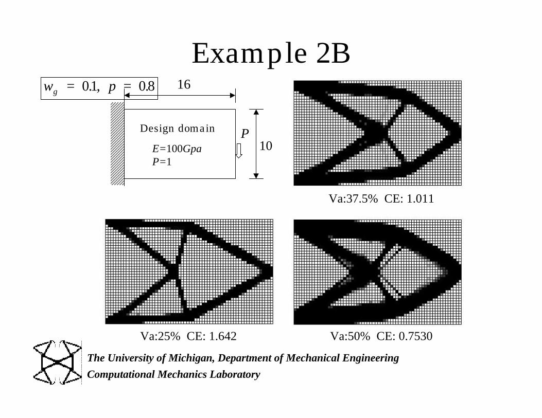
Example 2B

10

16


Va:37.5% CE: 1.011

Va:50% CE: 0.7530Va:25% CE: 1.642

w pg = =01 0 8. , .



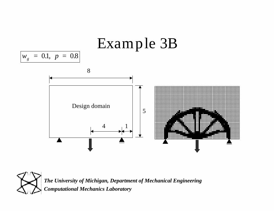
Example 3B

Design domain

4 1

8

5

w pg = =01 0 8. , .



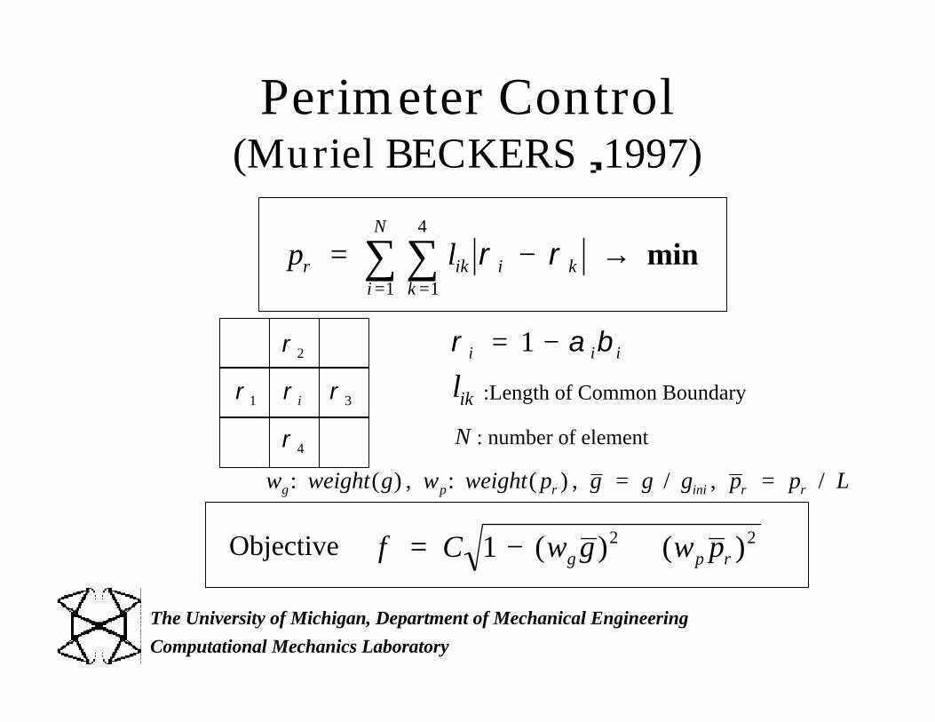
Perimeter Control(Muriel BECKERS，1997)

ρ i

ρ2

ρ1 ρ 3

ρ4

ρ α βi i i= −1

lik :Length of Common Boundary

p lr ik i kki

N

= − →==

∑∑ ρ ρ1

4

1

min

w weight g w weight p g g g p p Lg p r ini r r: ( ) , : ( ) , / , /= =

N : number of element

f C w g w pg p r= − +1 2 2( ) ( )Objective



Perimeter Length

pri = 0 pri = 1 pri = 2 pri = 3 pri = 4

ρ i = 1

ρ i = 0 5.

pri = 0 pri = 0 5. pri = 1 pri = 15. pri = 2

ρ i = 0

pri = 4 pri = 3 pri = 2 pri = 1 pri = 0



Example 1C

24

10

PDesignDomain

Va: 10% Va: 20% Va: 30%

w p wg p= = =01 08 0 01. , . , .



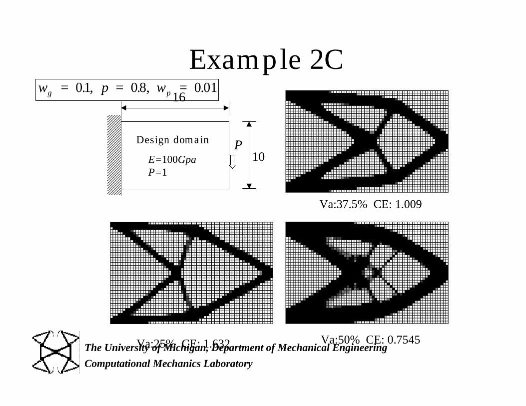
Example 2C

10

16


Va:37.5% CE: 1.009

Va:50% CE: 0.7545Va:25% CE: 1.632

w p wg p= = =01 08 0 01. , . , .



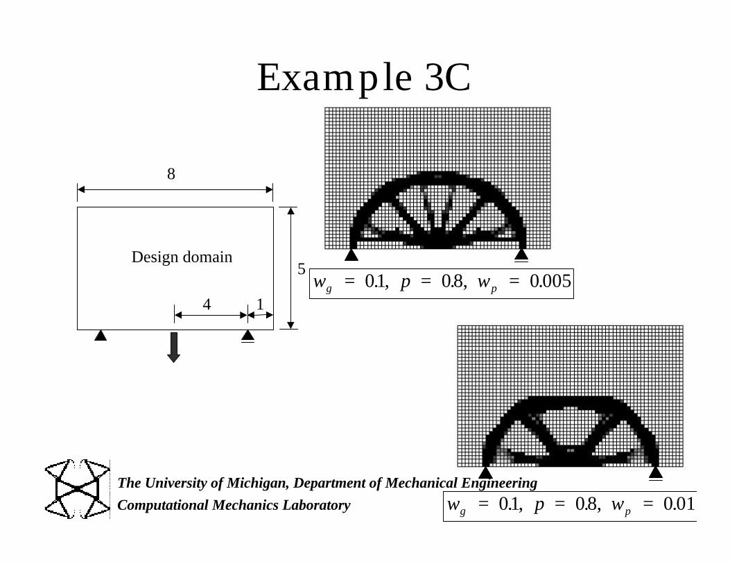
Example 3C

Design domain

4 1

8

5

w p wg p= = =01 08 0 01. , . , .

w p wg p= = =01 08 0 005. , . , .



Post Processingof

OPTISHAPE

Smooth Surface Extruction



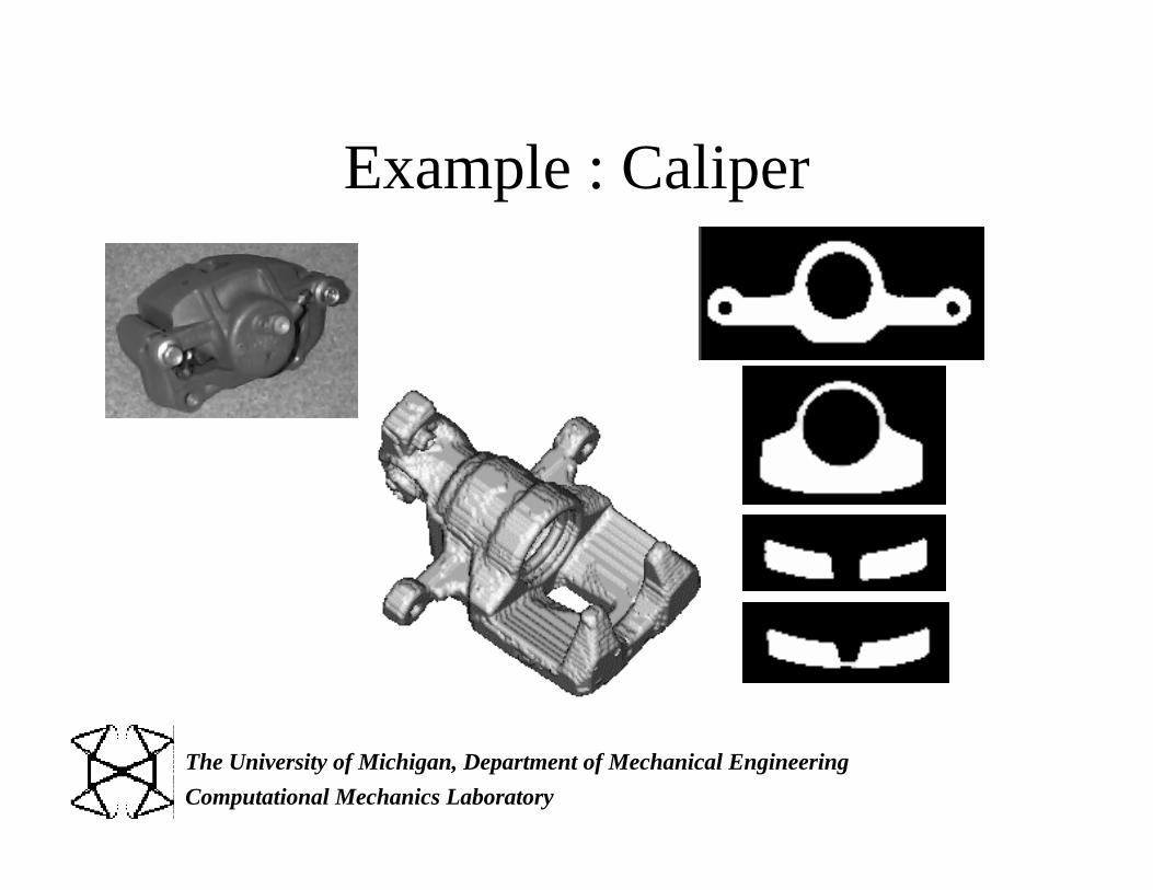
Example : Caliper



OPTISHAPE

Mesh From CT Scan150,000 3-D Elements 9% Weight Reduction



Comparison by Sections



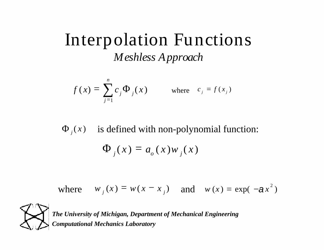
Interpolation FunctionsMeshless Approach

f ( x) = c jj =1

n

∑ Φ j ( x )

Φ j ( x ) = ao ( x )w j ( x )

c j = f ( x j )where

Φ j ( x ) is defined with non-polynomial function:

where w j (x ) = w ( x − x j ) w (x ) = exp( −αx 2 )and



Approximation Functions (2)

Φ j ( x ) = ao ( x ) + x ja 1 ( x ) + K + x j

k a k ( x ) w j ( x)

= 1 K x j

k ao ( x )

M

a k ( x )

w j ( x )

f ( x) = fo + f1 x + K + fk xk

To Determine which yield k-th degree polynomial,let’s assume:

Φ j ( x )

Solve for a o ( x ) K a k ( x )

f ( x) = c jj =1

n

∑ Φj ( x )



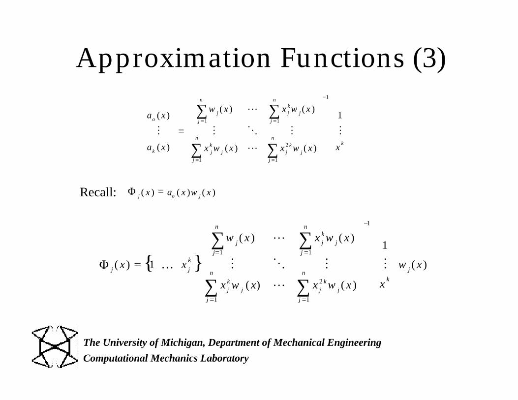
Approximation Functions (3)

ao ( x )

M

ak ( x )

=

w j ( x )j =1

n

∑ L x jk w j ( x )

j =1

n

∑M O M

x jk w j ( x )

j =1

n

∑ L x j2 k w j ( x )

j =1

n

∑

−1

1

M

x k

Φ j ( x ) = 1 K x j

k w j ( x )

j=1

n

∑ L x jk w j ( x )

j =1

n

∑M O M

x jk w j ( x)

j =1

n

∑ L x j2 k w j ( x )

j =1

n

∑

−1

1

M

x k

w j ( x )

Φ j ( x ) = ao ( x )w j ( x )Recall:



Reconstruction of a 3-D Model

χΩh ( x, y, z ) = χ Ω,k

h ( x , y )k =1

k max

∑ Φ k ( z)

χΩ ,k

h

Φ k (z )

: Characteristic function of each image Greyscale values (0-255)

: Approximation functions

2D image Basis Functions



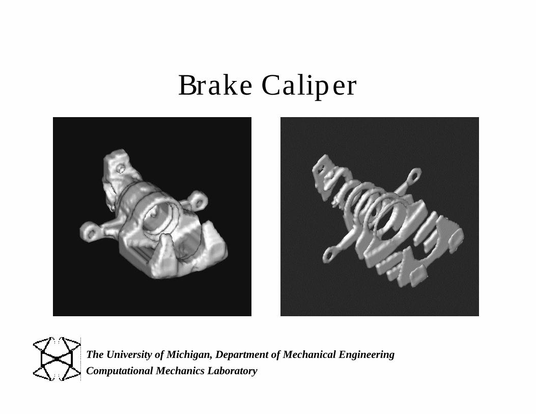
Brake Caliper



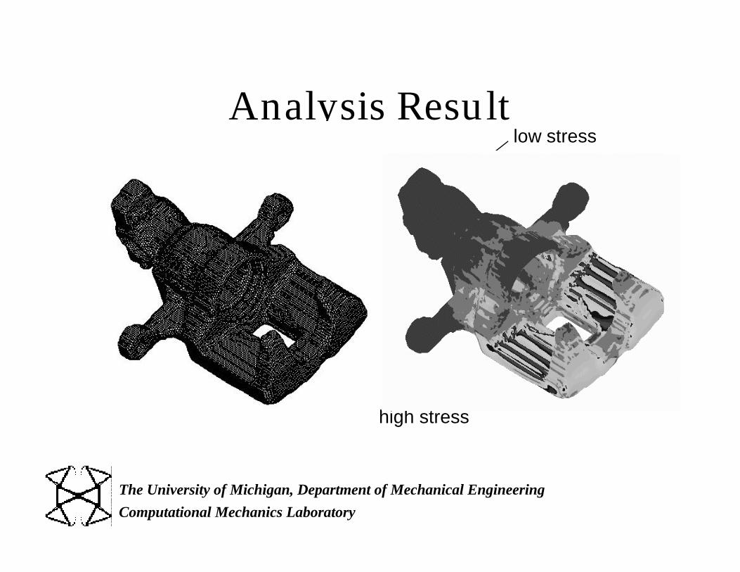
Analysis Resultlow stress

high stress



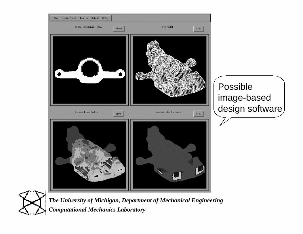
Possibleimage-baseddesign software



Optimization



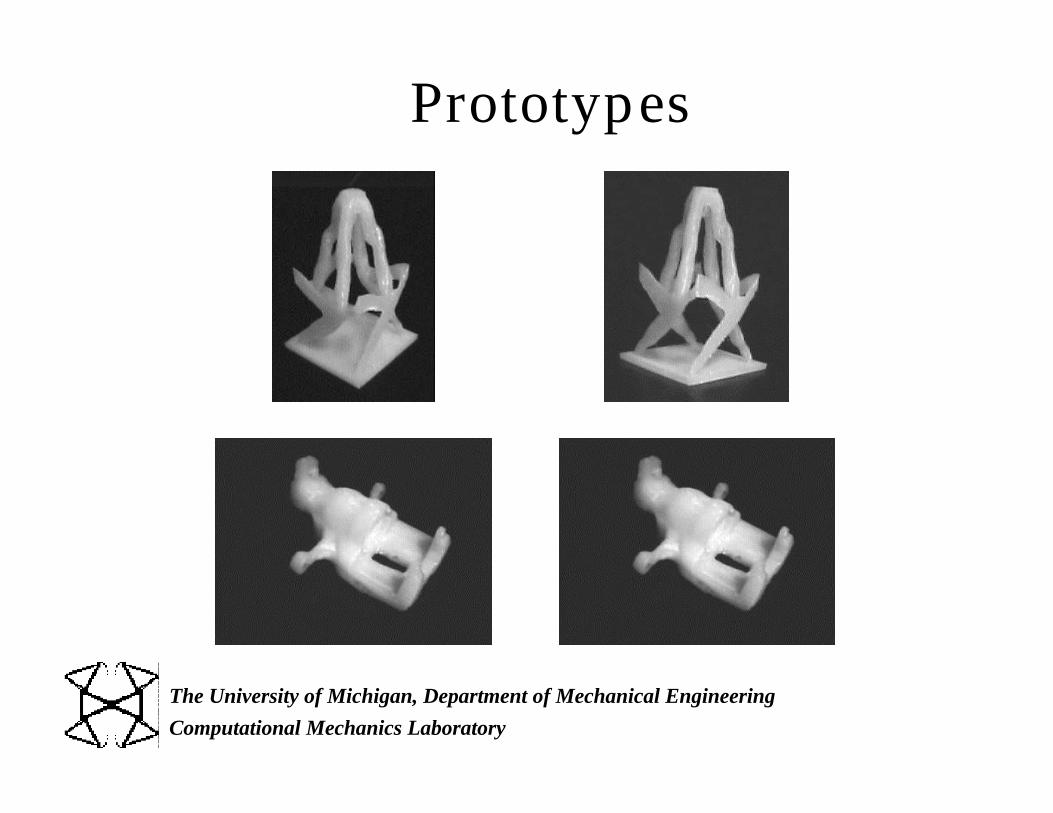
Prototypes



Summary

Concept of OPTISHAPE : TopologyOptimization is continuously extended not

only to structures but also materials,mechanisms, electro-magnetic fields, and

others



VOXELCON for I-DEASOPTISHAPE for I-DEAS

NASTRAN-OPTISHAPE

TowardImage Based CAE

Date post:	23-Oct-2021
Category:	Documents
Upload:	others
View:	2 times
Download:	0 times

Emerging Technology in Optimization

Documents